Numerical and Experimental Investigation of Heat Transfer ...
1/59
Instructor Wen-Quan Tao; Qinlong Ren; Li Chen
CFD-NHT-EHT Center
Key Laboratory of Thermo-Fluid Science & Engineering
Xi’an Jiaotong University
Xi’an, 2018-Dec.-12
Numerical Heat Transfer
Chapter 13 Application examples of fluent for basic flow and heat transfer problem
2/59
数值传热学第 13 章 求解流动换热问题的Fluent软件基础应用举例
主讲 陶文铨
西安交通大学能源与动力工程学院热流科学与工程教育部重点实验室
2018年12月12日, 西安
辅讲 任秦龙,陈 黎
3/59
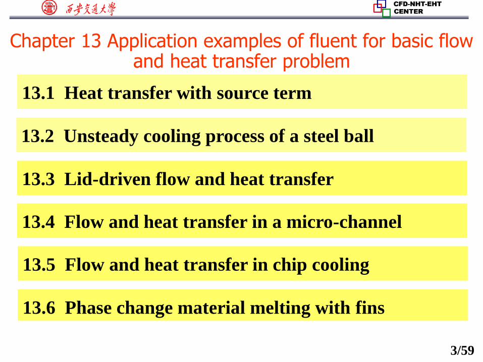
13.2 Unsteady cooling process of a steel ball
13.3 Lid-driven flow and heat transfer
13.5 Flow and heat transfer in chip cooling
13.1 Heat transfer with source term
13.4 Flow and heat transfer in a micro-channel
Chapter 13 Application examples of fluent for basic flow and heat transfer problem
13.6 Phase change material melting with fins
4/59
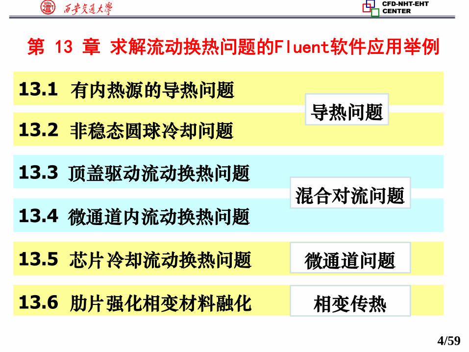
第 13 章 求解流动换热问题的Fluent软件应用举例
13.2 非稳态圆球冷却问题
13.3 顶盖驱动流动换热问题
13.5 芯片冷却流动换热问题
13.1 有内热源的导热问题
13.4 微通道内流动换热问题
导热问题
混合对流问题
微通道问题
13.6 肋片强化相变材料融化 相变传热
5/59
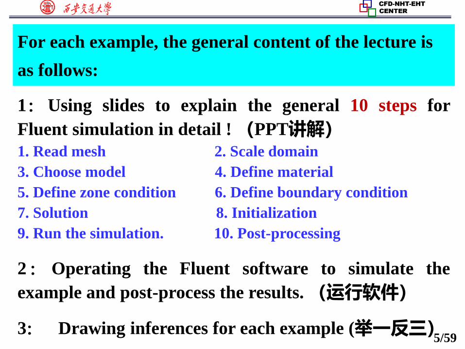
For each example, the general content of the lecture is
as follows:
2: Operating the Fluent software to simulate the
example and post-process the results. (运行软件)
1:Using slides to explain the general 10 steps for
Fluent simulation in detail ! (PPT讲解)1. Read mesh 2. Scale domain
3. Choose model 4. Define material
5. Define zone condition 6. Define boundary condition
7. Solution 8. Initialization
9. Run the simulation. 10. Post-processing
3: Drawing inferences for each example (举一反三)
6/59
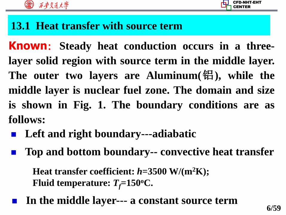
13.1 Heat transfer with source term
Known:Steady heat conduction occurs in a three-
layer solid region with source term in the middle layer.
The outer two layers are Aluminum(铝), while the
middle layer is nuclear fuel zone. The domain and size
is shown in Fig. 1. The boundary conditions are as
follows:
Top and bottom boundary-- convective heat transfer
Left and right boundary---adiabatic
Heat transfer coefficient: h=3500 W/(m2K);
Fluid temperature: Tf=150oC.
In the middle layer--- a constant source term
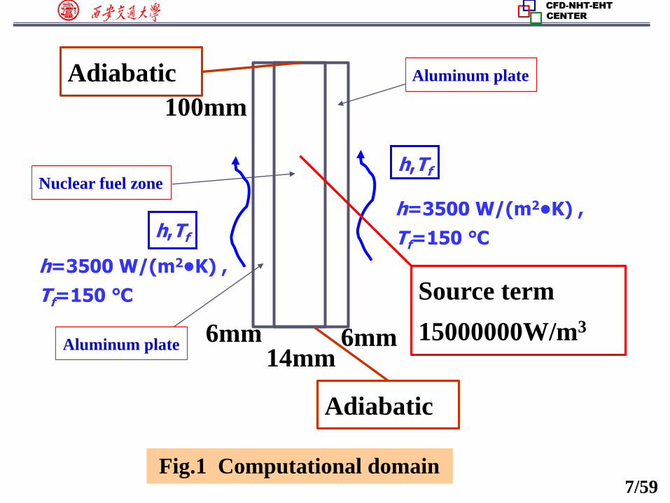
7/59Fig.1 Computational domain
Aluminum plate
Aluminum plate
Nuclear fuel zoneh,Tf
h,Tf
h=3500 W/(m2•K) ,
Tf=150 ℃
6mm 6mm14mm
100mm
Adiabatic
Adiabatic
Source term
15000000W/m3
h=3500 W/(m2•K) ,
Tf=150 ℃
8/59
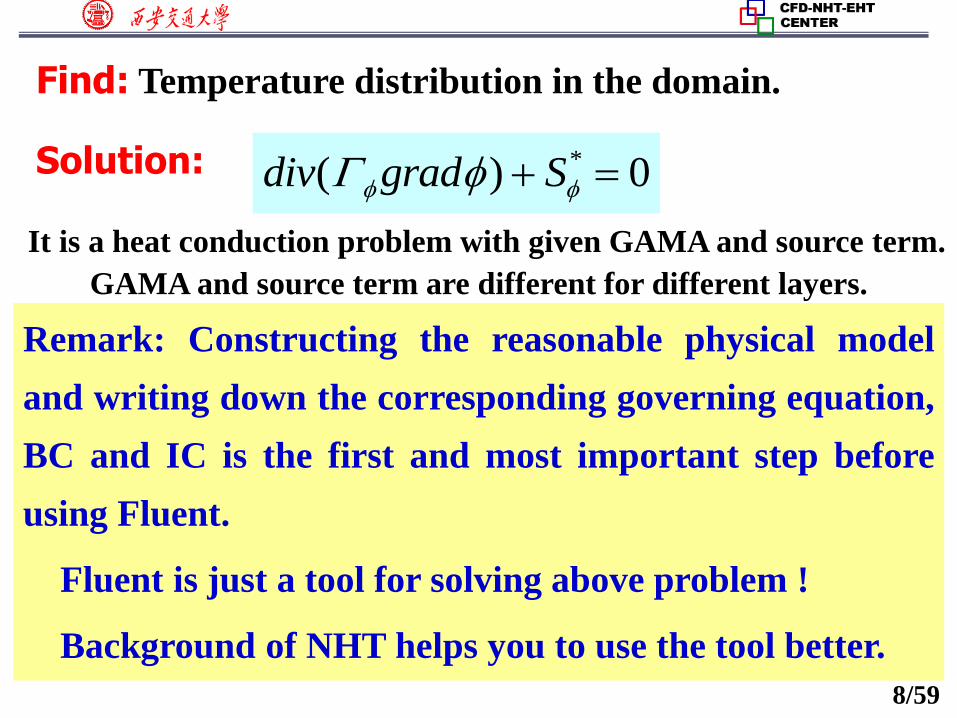
Solution: *( ) 0div grad S
It is a heat conduction problem with given GAMA and source term.
GAMA and source term are different for different layers.
Find: Temperature distribution in the domain.
Remark: Constructing the reasonable physical model
and writing down the corresponding governing equation,
BC and IC is the first and most important step before
using Fluent.
Fluent is just a tool for solving above problem !
Background of NHT helps you to use the tool better.
9/59
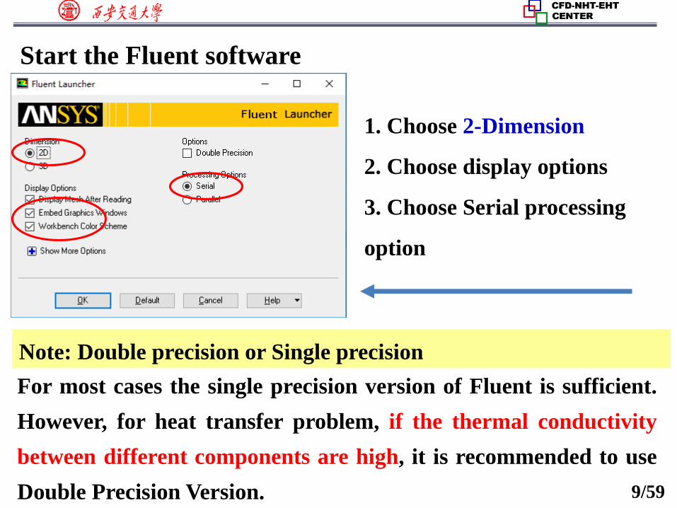
Start the Fluent software
1. Choose 2-Dimension
2. Choose display options
3. Choose Serial processing
option
Note: Double precision or Single precision
For most cases the single precision version of Fluent is sufficient.
However, for heat transfer problem, if the thermal conductivity
between different components are high, it is recommended to use
Double Precision Version.
10/59
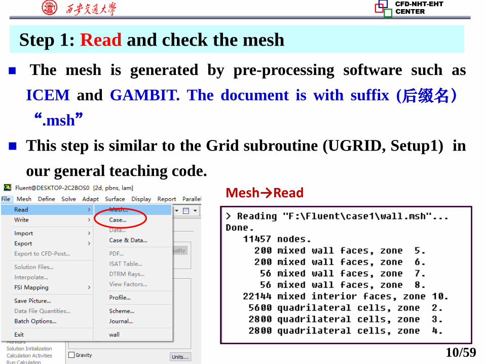
Step 1: Read and check the mesh
The mesh is generated by pre-processing software such as
ICEM and GAMBIT. The document is with suffix (后缀名)
“.msh”
This step is similar to the Grid subroutine (UGRID, Setup1) in
our general teaching code.
Mesh→Read
11/59
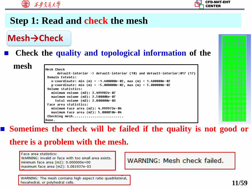
Step 1: Read and check the mesh
Mesh→Check
Check the quality and topological information of the
mesh
Sometimes the check will be failed if the quality is not good or
there is a problem with the mesh.
12/59
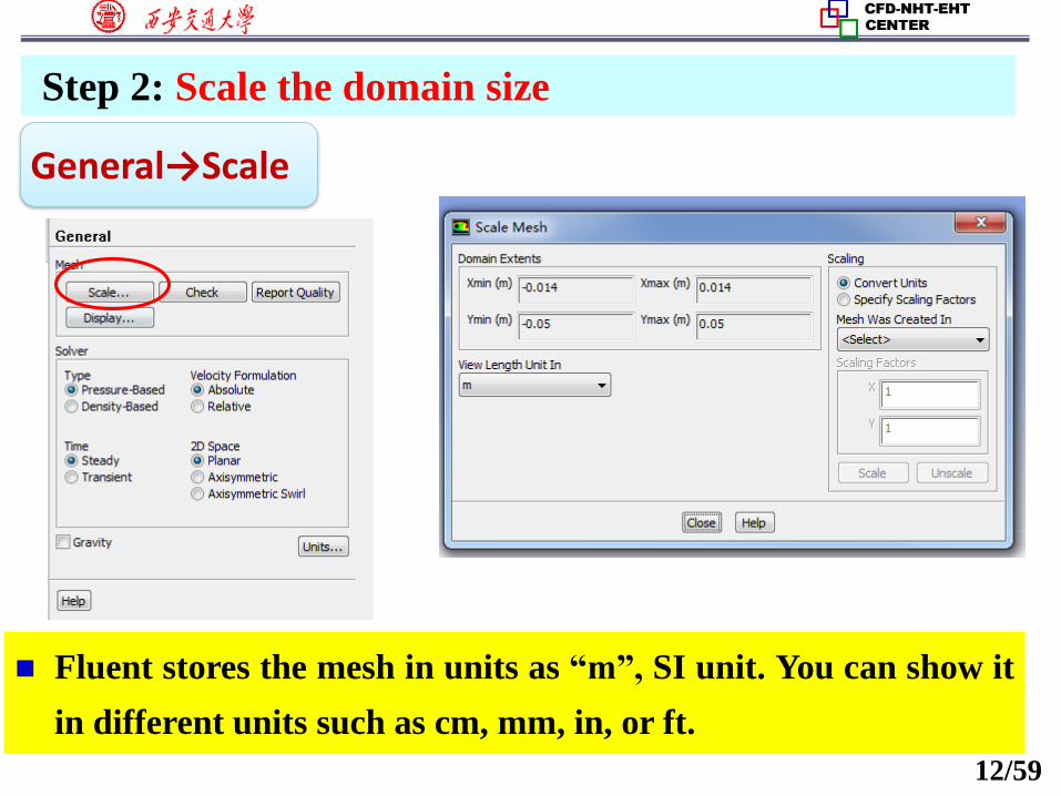
Step 2: Scale the domain size
Fluent stores the mesh in units as “m”, SI unit. You can show it
in different units such as cm, mm, in, or ft.
General→Scale
13/59
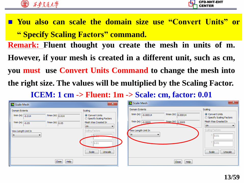
You also can scale the domain size use “Convert Units” or
“ Specify Scaling Factors” command.
Remark: Fluent thought you create the mesh in units of m.
However, if your mesh is created in a different unit, such as cm,
you must use Convert Units Command to change the mesh into
the right size. The values will be multiplied by the Scaling Factor.
ICEM: 1 cm -> Fluent: 1m -> Scale: cm, factor: 0.01
14/59
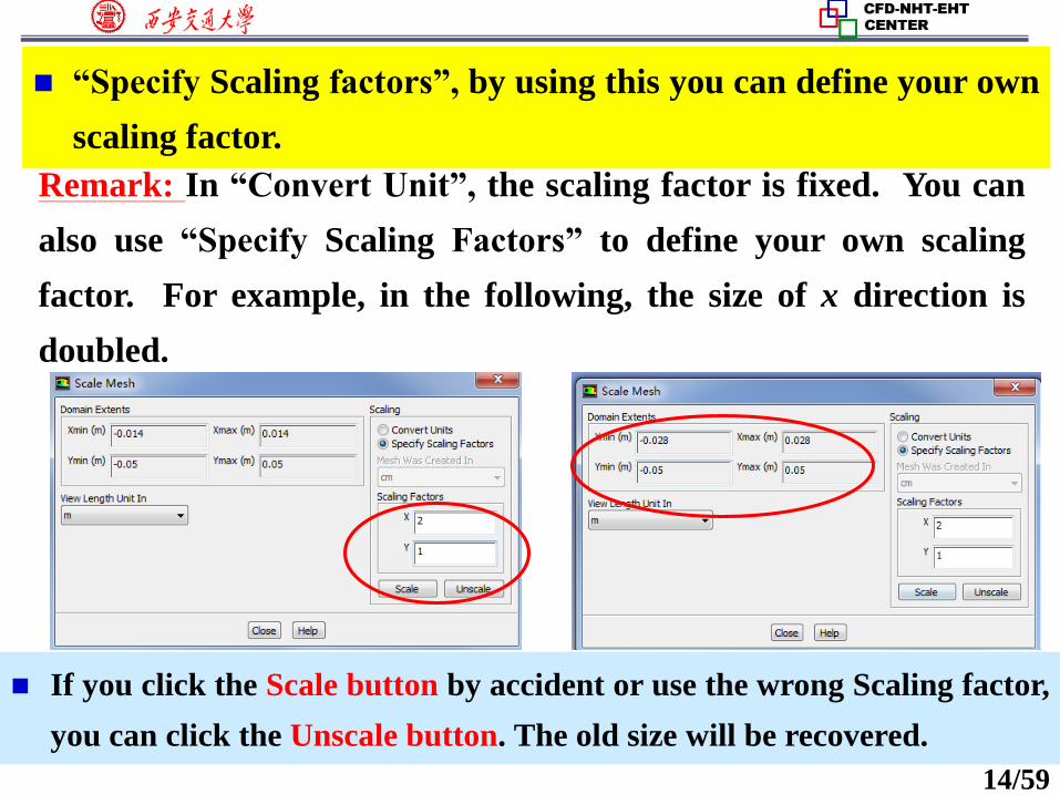
“Specify Scaling factors”, by using this you can define your own
scaling factor.
Remark: In “Convert Unit”, the scaling factor is fixed. You can
also use “Specify Scaling Factors” to define your own scaling
factor. For example, in the following, the size of x direction is
doubled.
If you click the Scale button by accident or use the wrong Scaling factor,
you can click the Unscale button. The old size will be recovered.
15/59
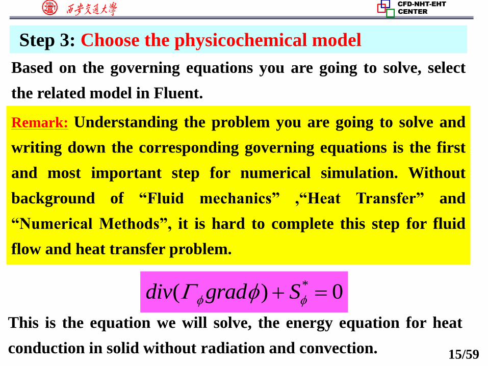
Step 3: Choose the physicochemical model
Based on the governing equations you are going to solve, select
the related model in Fluent.
Remark: Understanding the problem you are going to solve and
writing down the corresponding governing equations is the first
and most important step for numerical simulation. Without
background of “Fluid mechanics” ,“Heat Transfer” and
“Numerical Methods”, it is hard to complete this step for fluid
flow and heat transfer problem.
*( ) 0div grad S
This is the equation we will solve, the energy equation for heat
conduction in solid without radiation and convection.
16/59
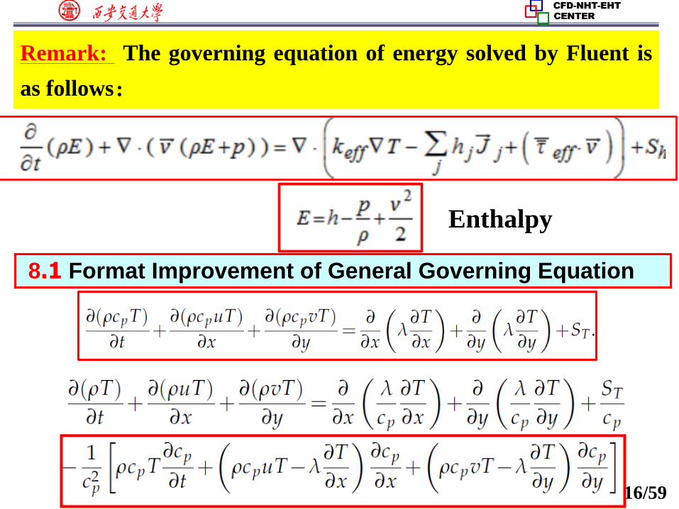
Remark: The governing equation of energy solved by Fluent is
as follows:
8.1 Format Improvement of General Governing Equation
Enthalpy
17/59
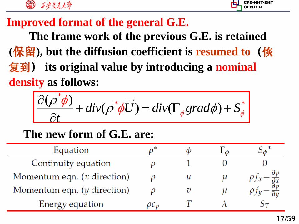
Improved format of the general G.E.
The frame work of the previous G.E. is retained
(保留), but the diffusion coefficient is resumed to(恢
复到) its original value by introducing a nominal
density as follows:*
* *( )( ) ( )div U div grad S
t
The new form of G.E. are:
18/59
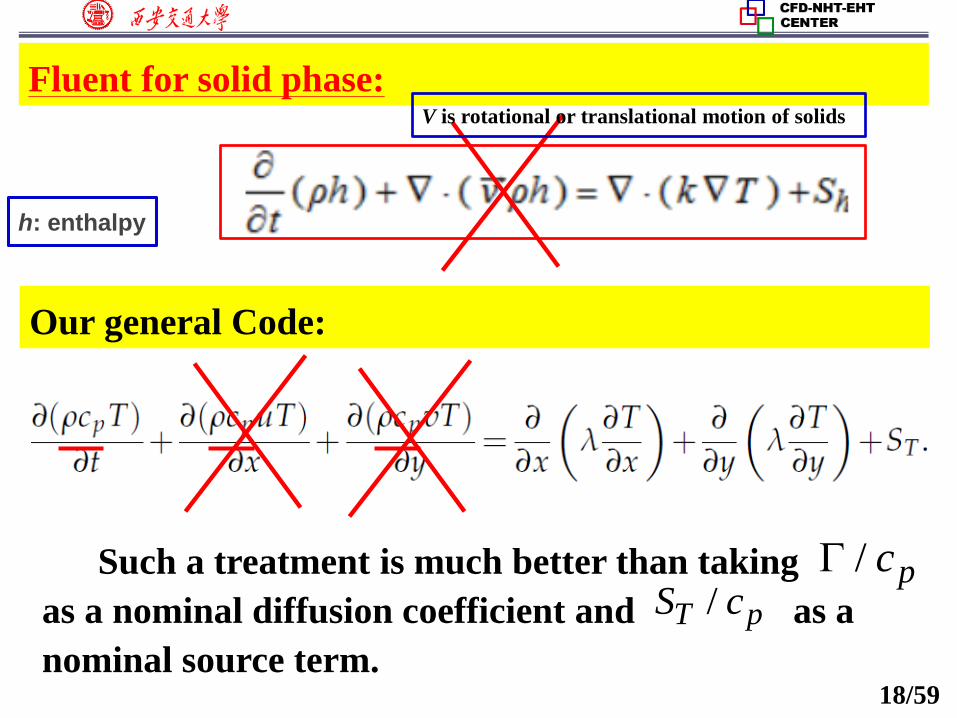
Fluent for solid phase:
Our general Code:
Such a treatment is much better than taking
as a nominal diffusion coefficient and as a
nominal source term.
/ pc/T pS c
V is rotational or translational motion of solids
h: enthalpy
19/59
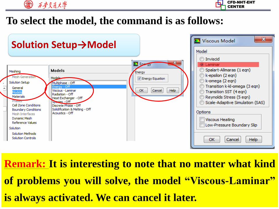
To select the model, the command is as follows:
Remark: It is interesting to note that no matter what kind
of problems you will solve, the model “Viscous-Laminar”
is always activated. We can cancel it later.
Solution Setup→Model
20/59
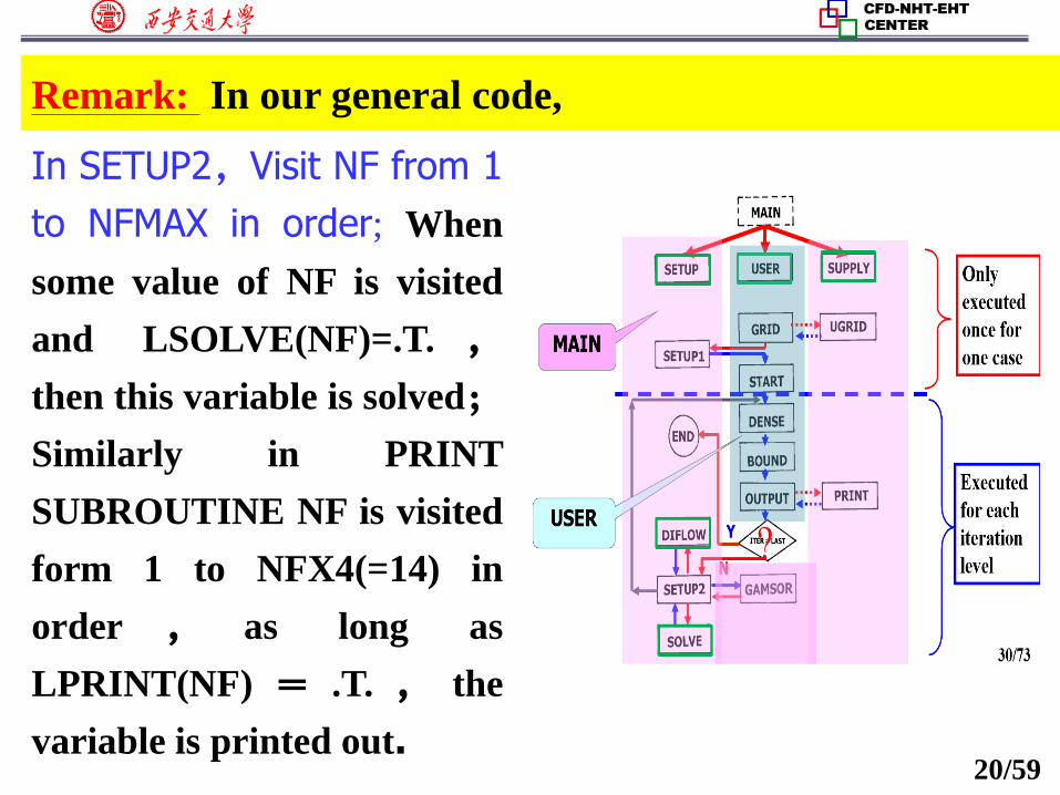
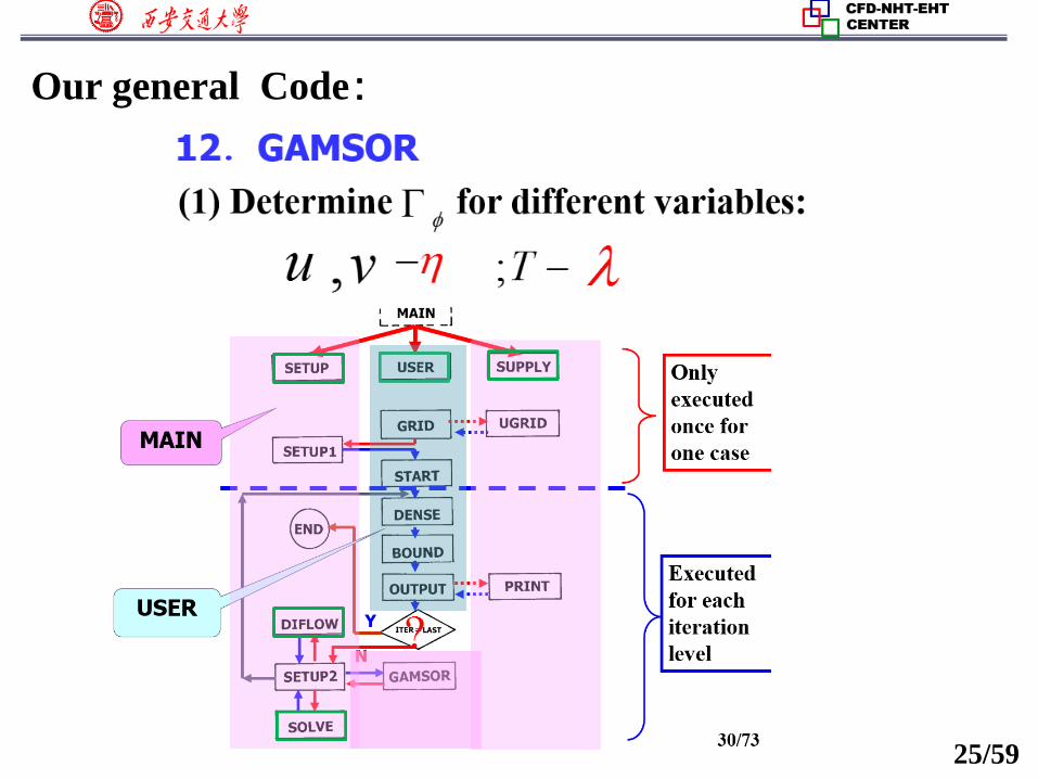
Remark: In our general code,
In SETUP2,Visit NF from 1
to NFMAX in order; When
some value of NF is visited
and LSOLVE(NF)=.T. ,
then this variable is solved;
Similarly in PRINT
SUBROUTINE NF is visited
form 1 to NFX4(=14) in
order , as long as
LPRINT(NF) = .T. , the
variable is printed out.
21/73
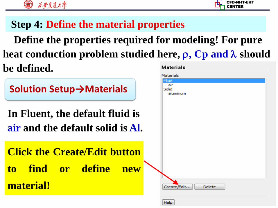
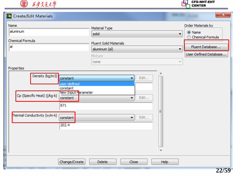
Step 4: Define the material properties
Define the properties required for modeling! For pure
heat conduction problem studied here, , Cp and should
be defined.
Solution Setup→Materials
In Fluent, the default fluid is
air and the default solid is Al.
Click the Create/Edit button
to find or define new
material!
22/59
23/59
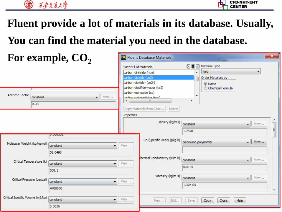
Fluent provide a lot of materials in its database. Usually,
You can find the material you need in the database.
For example, CO2
24/59
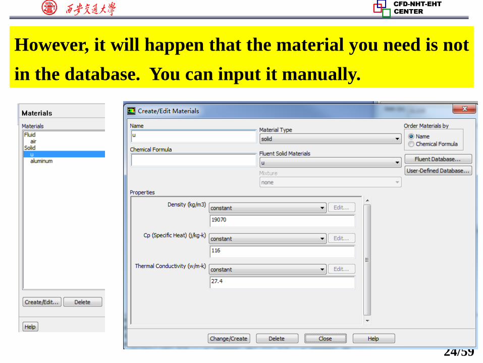
However, it will happen that the material you need is not
in the database. You can input it manually.
25/59
Our general Code:
26/59
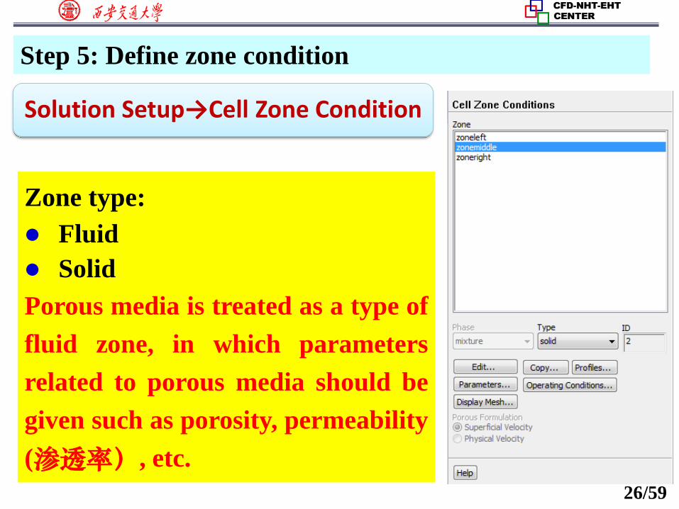
Step 5: Define zone condition
Solution Setup→Cell Zone Condition
Zone type:
Fluid
Solid
Porous media is treated as a type of
fluid zone, in which parameters
related to porous media should be
given such as porosity, permeability
(渗透率), etc.
27/59
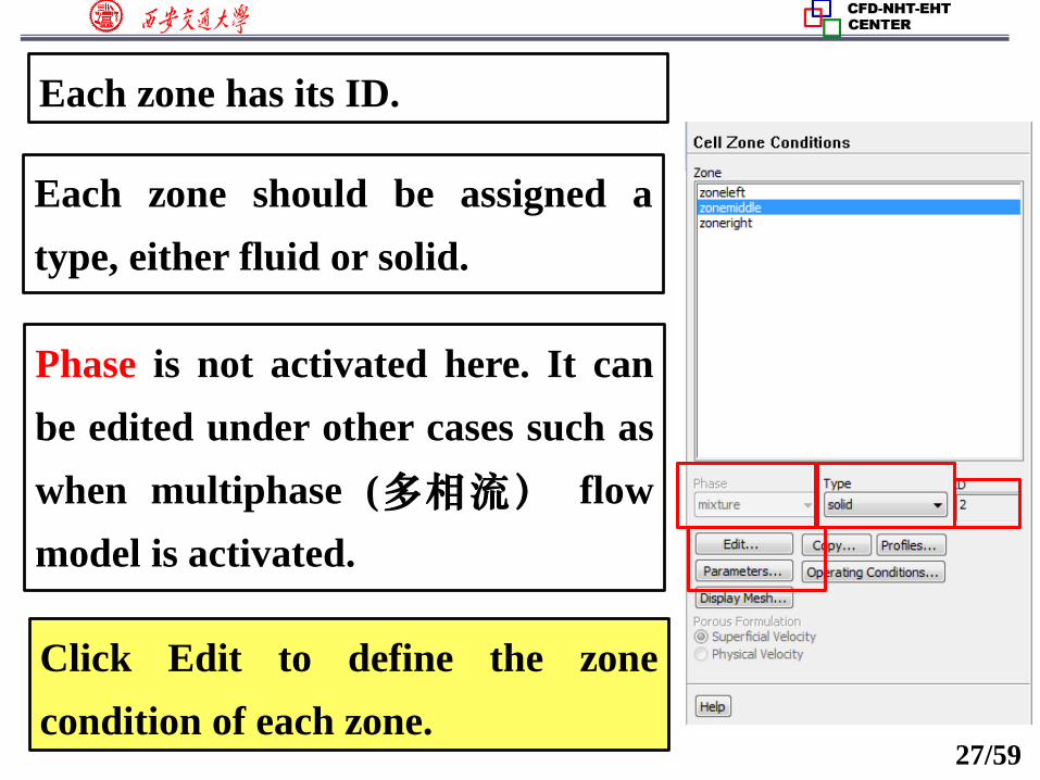
Each zone has its ID.
Each zone should be assigned a
type, either fluid or solid.
Phase is not activated here. It can
be edited under other cases such as
when multiphase (多相流) flow
model is activated.
Click Edit to define the zone
condition of each zone.
28/59
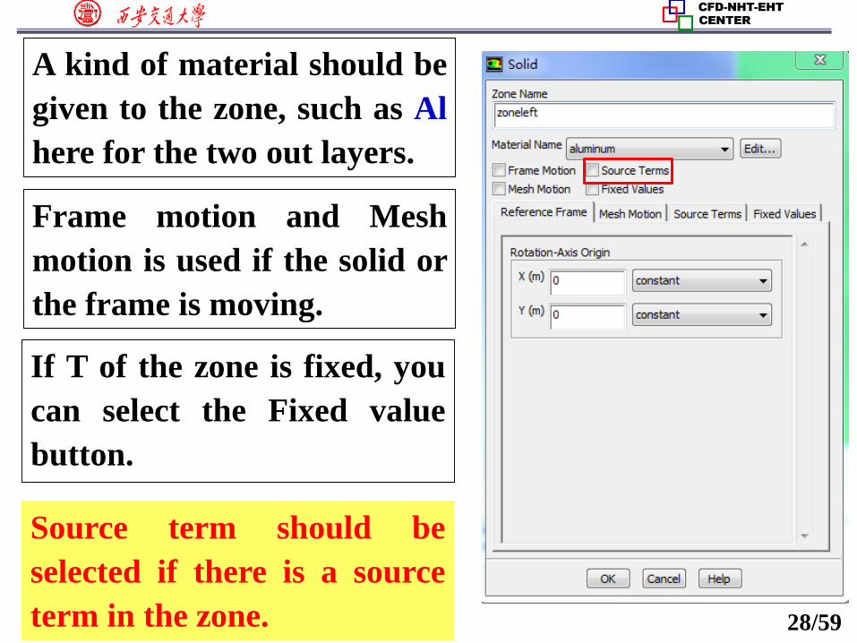
A kind of material should be
given to the zone, such as Al
here for the two out layers.
Source term should be
selected if there is a source
term in the zone.
Frame motion and Mesh
motion is used if the solid or
the frame is moving.
If T of the zone is fixed, you
can select the Fixed value
button.
29/73
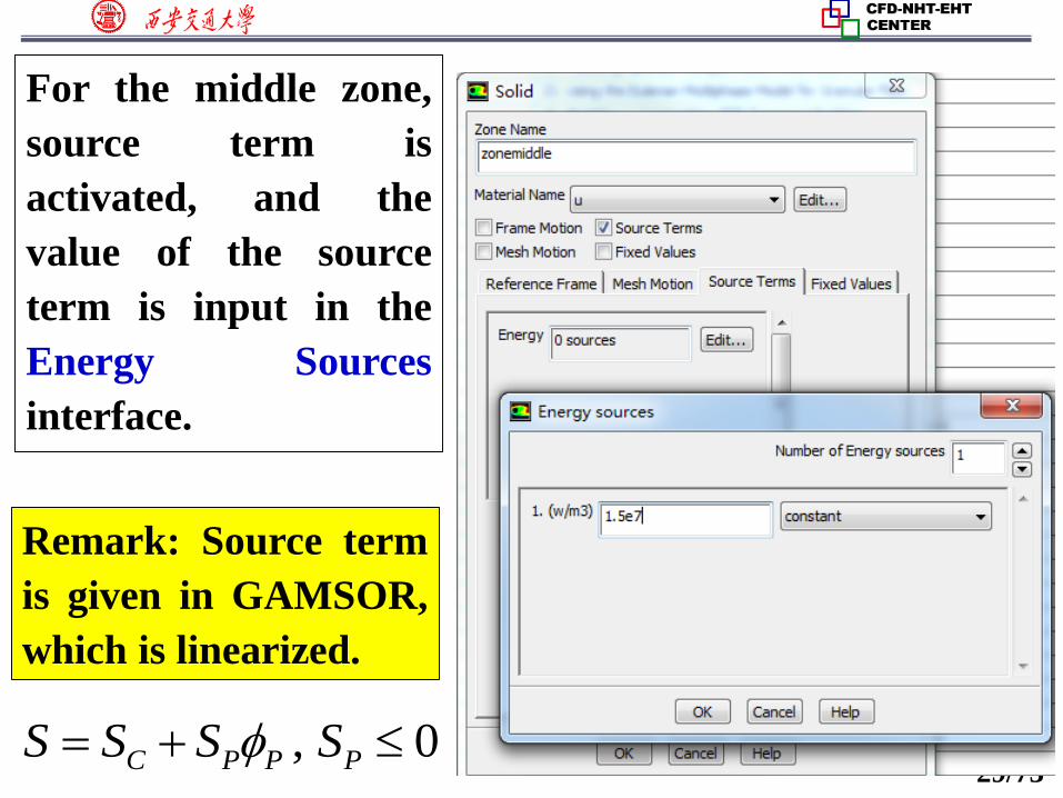
For the middle zone,
source term is
activated, and the
value of the source
term is input in the
Energy Sources
interface.
Remark: Source term
is given in GAMSOR,
which is linearized.
, 0C P P PS S S S

30/59
Remark: In Fluent, if the source term is not a constant
and is a function of the variable solved, local
linearization of source term is also adopted.
, 0C P P PS S S S
Specifying a value for 𝑆𝑝 can enhance the stability of the
solution and help convergence rates due to the increase
in diagonal terms on the solution matrix.
For general source term that is not a constant, user
defined function (UDF) is required in Fluent.
Define_Source is adopted to specify custom source term
for different transport equations.
𝑆𝑐 = 𝑆∗ − Τ𝜕𝑆 𝜕∅ ∗∅∗, 𝑆𝑝 = Τ𝜕𝑆 𝜕∅ ∗
31/59
Step 6: Define the boundary condition
Boundary condition definition is one of the most
important and difficult step during Fluent simulation.
General boundary conditions in Fluent can be divided
into two kinds:
1. BC at inlet and outlet: pressure, velocity, mass flow
rate, outflow…
2. BC at wall: wall, periodic, symmetric…
Remark: Interior cell zone and interior interface will
also shown in the BC Window.
32/59
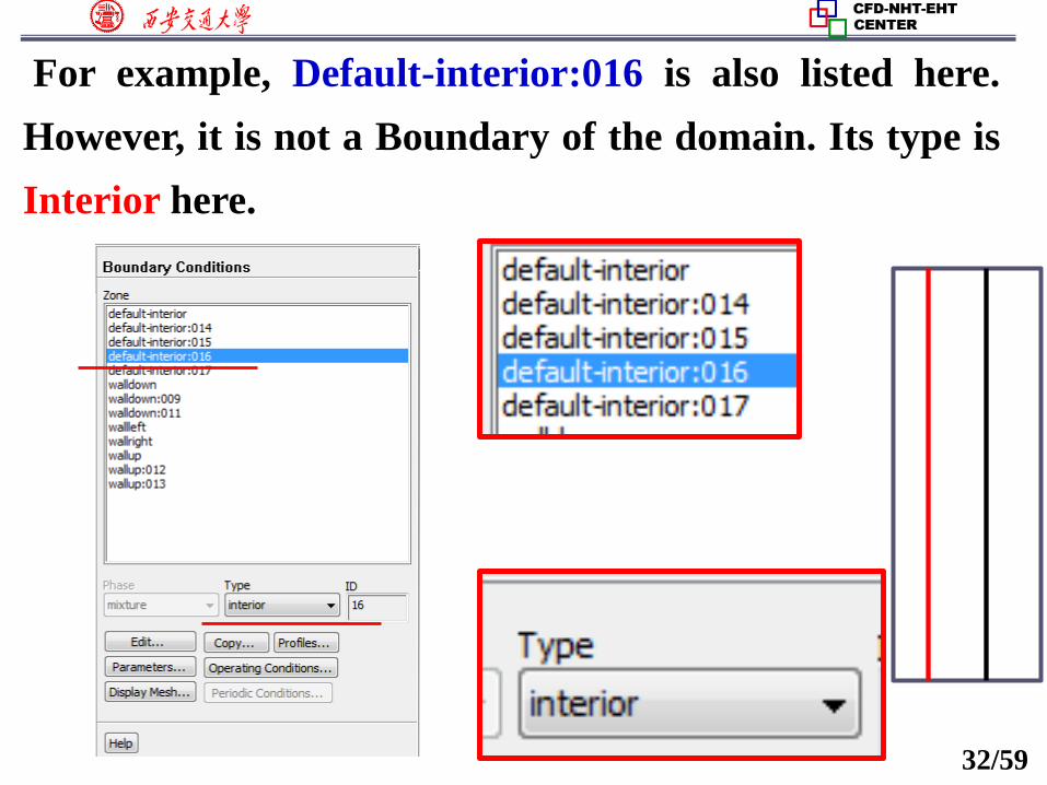
For example, Default-interior:016 is also listed here.
However, it is not a Boundary of the domain. Its type is
Interior here.

33/59
Here, only the BCs related to the heat conduction
problem studied here are introduced. Other types of
BCs will be introduced in other examples.
Solution Setup→Boundary conditions
34/59
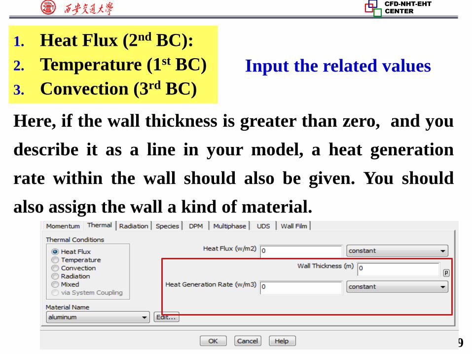
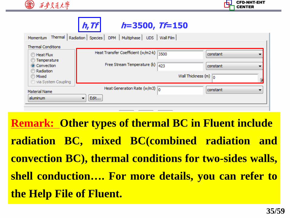
1. Heat Flux (2nd BC):
2. Temperature (1st BC)
3. Convection (3rd BC)
Here, if the wall thickness is greater than zero, and you
describe it as a line in your model, a heat generation
rate within the wall should also be given. You should
also assign the wall a kind of material.
Input the related values
35/59
h,Tf h=3500, Tf=150
Remark: Other types of thermal BC in Fluent include
radiation BC, mixed BC(combined radiation and
convection BC), thermal conditions for two-sides walls,
shell conduction…. For more details, you can refer to
the Help File of Fluent.
36/59
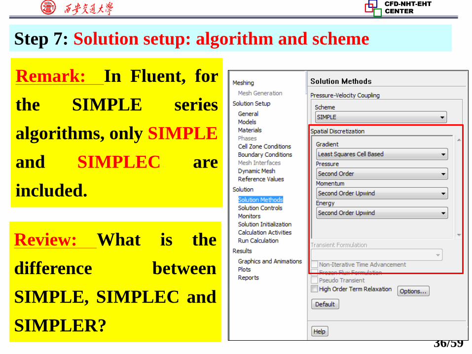
Step 7: Solution setup: algorithm and scheme
Remark: In Fluent, for
the SIMPLE series
algorithms, only SIMPLE
and SIMPLEC are
included.
Review: What is the
difference between
SIMPLE, SIMPLEC and
SIMPLER?
37/59
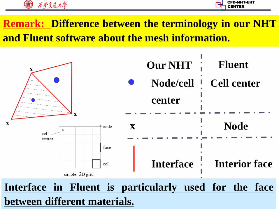
Remark: Difference between the terminology in our NHT
and Fluent software about the mesh information.
Our NHT Fluent
Node/cell
center
Cell center
x Node
Interface Interior face
Interface in Fluent is particularly used for the face
between different materials.
38/59
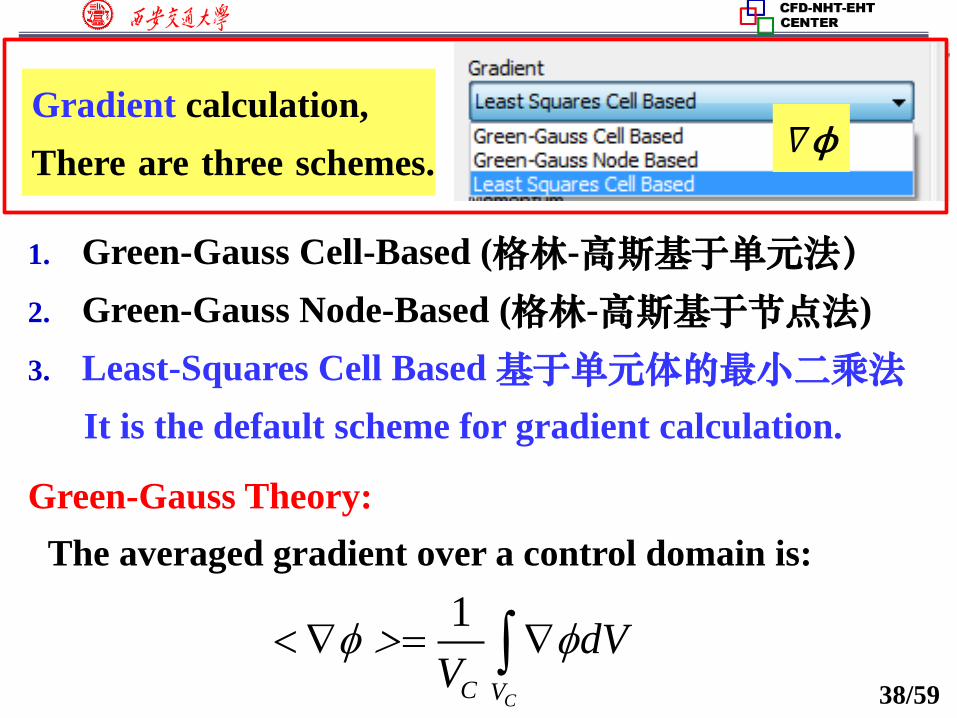
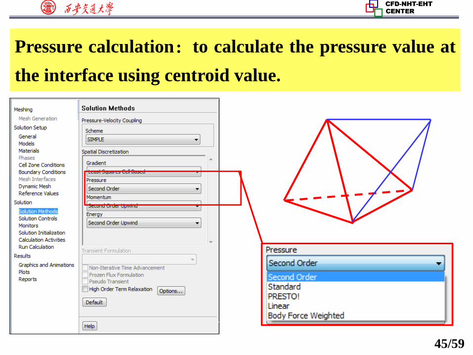
Gradient calculation,
There are three schemes.
1. Green-Gauss Cell-Based (格林-高斯基于单元法)
2. Green-Gauss Node-Based (格林-高斯基于节点法)
3. Least-Squares Cell Based基于单元体的最小二乘法
It is the default scheme for gradient calculation.
1
CC V
dVV
Green-Gauss Theory:
The averaged gradient over a control domain is:
𝛻ϕ
39/59
1 1
CC CV
dV dSV V
n
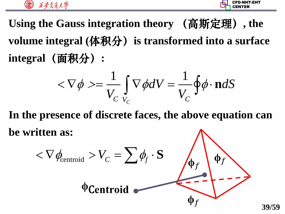
Using the Gauss integration theory (高斯定理), the
volume integral (体积分)is transformed into a surface
integral(面积分):
In the presence of discrete faces, the above equation can
be written as:
centroid C fV S ϕ𝑓
ϕ𝑓
ϕ𝑓
ϕCentroid
40/59
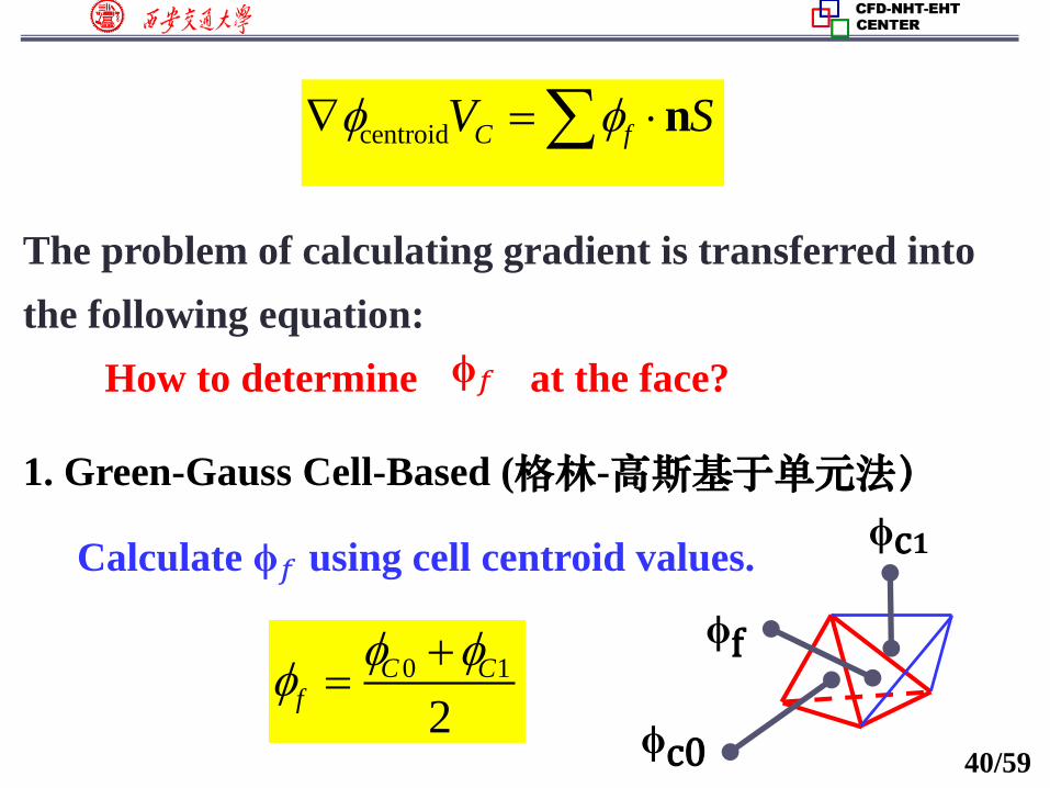
The problem of calculating gradient is transferred into
the following equation:
How to determine at the face?ϕ𝑓
centroid C fV S n
1. Green-Gauss Cell-Based (格林-高斯基于单元法)
Calculate ϕ𝑓 using cell centroid values.
0 1
2
C Cf
ϕc0
ϕc𝟏
ϕf
41/59
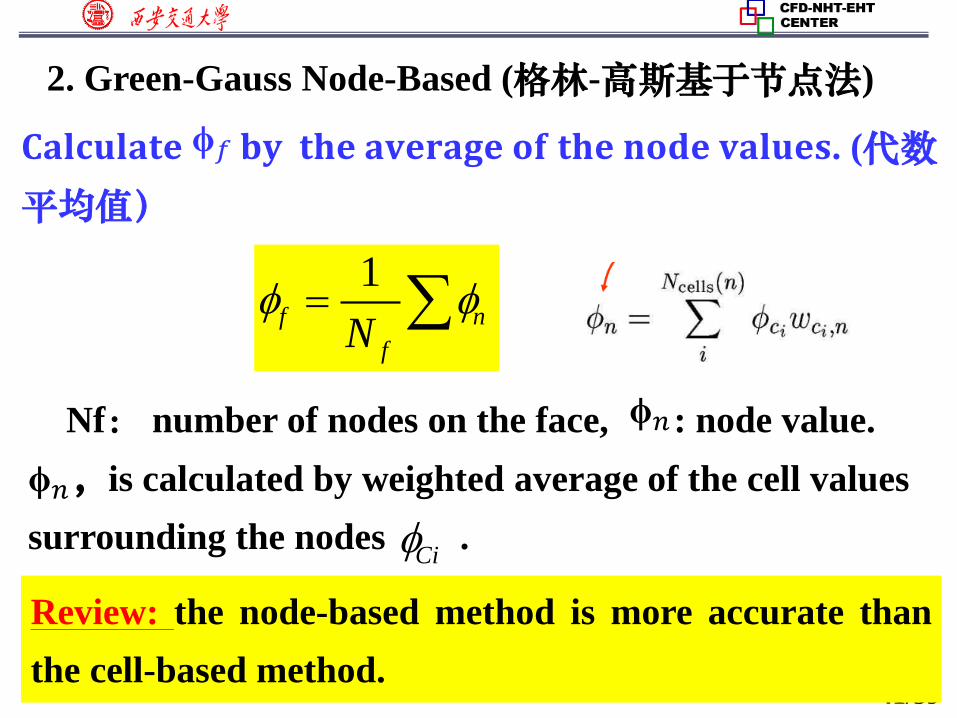
2. Green-Gauss Node-Based (格林-高斯基于节点法)
𝐂𝐚𝐥𝐜𝐮𝐥𝐚𝐭𝐞 𝐛𝐲 𝐭𝐡𝐞 𝐚𝐯𝐞𝐫𝐚𝐠𝐞 𝐨𝐟 𝐭𝐡𝐞 𝐧𝐨𝐝𝐞 𝐯𝐚𝐥𝐮𝐞𝐬. (代数
平均值)
1f n
fN
ϕ𝑓
Nf: number of nodes on the face, : node value.ϕ𝑛
ϕ𝑛,is calculated by weighted average of the cell values
surrounding the nodes .
Review: the node-based method is more accurate than
the cell-based method.
Ci
42/59
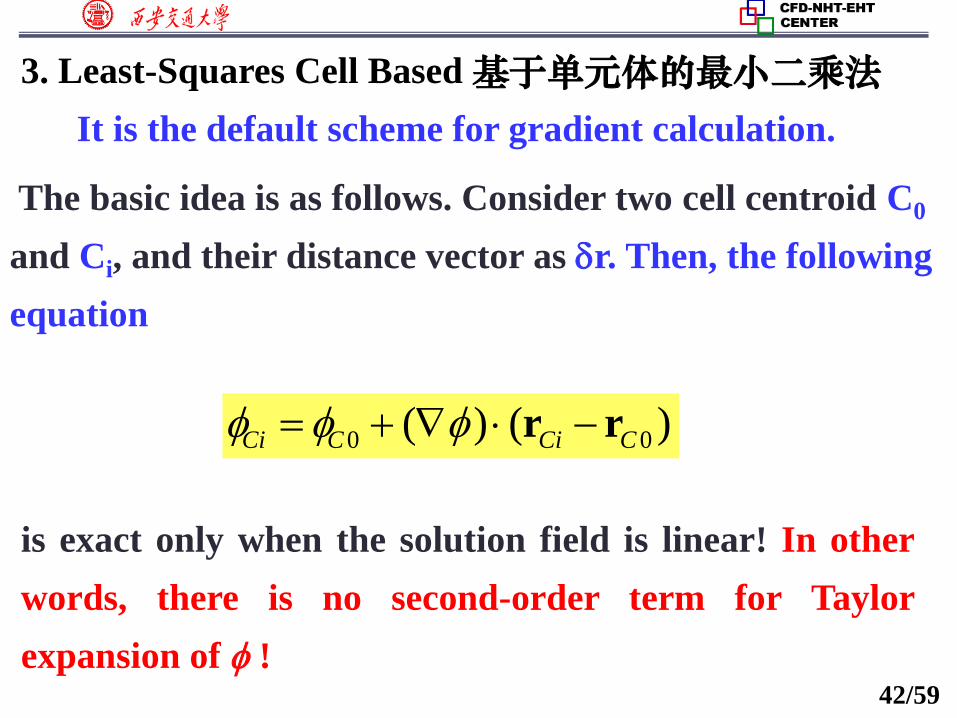
3. Least-Squares Cell Based基于单元体的最小二乘法
It is the default scheme for gradient calculation.
The basic idea is as follows. Consider two cell centroid C0
and Ci, and their distance vector as r. Then, the following
equation
0 0( ) ( )Ci C Ci C r r
is exact only when the solution field is linear! In other
words, there is no second-order term for Taylor
expansion of !
43/59
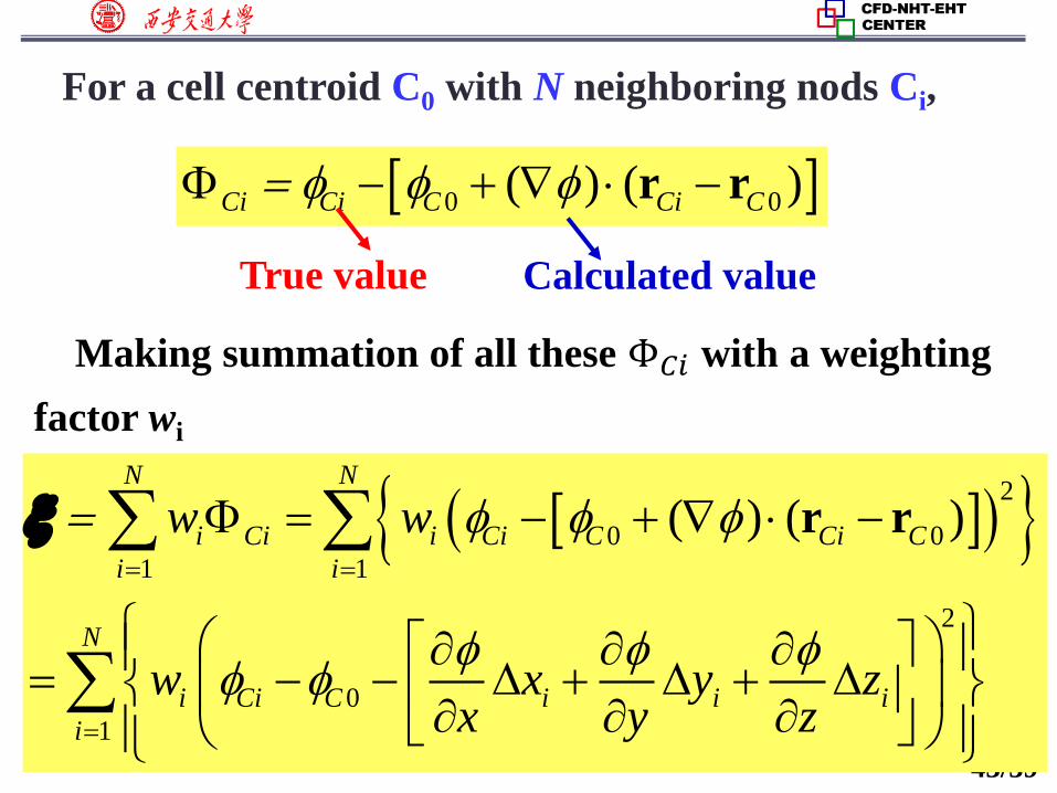
For a cell centroid C0 with N neighboring nods Ci,
0 0( ) ( )Ci Ci C Ci C r r
Making summation of all these Φ𝐶𝑖 with a weighting
factor wi
2
0 0
1 1
2
0
1
( ) ( )N N
i Ci i Ci C Ci C
i i
N
i Ci C i i i
i
w w
w x y zx y z
r r
True value Calculated value
44/59
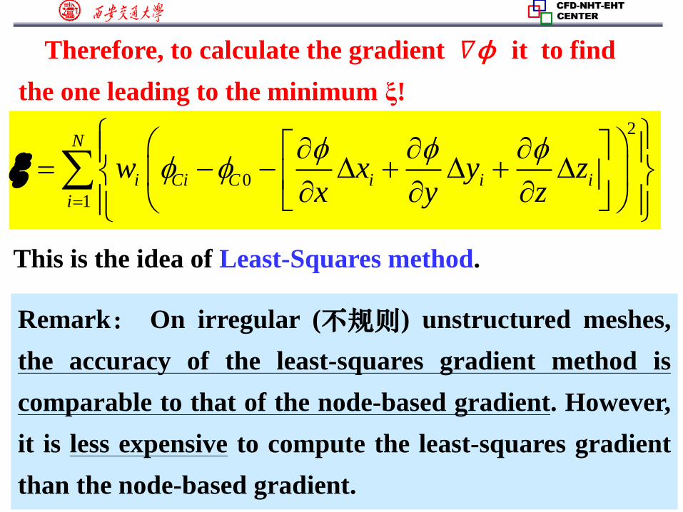
Therefore, to calculate the gradient it to find
the one leading to the minimum ξ!
𝛻ϕ
2
0
1
N
i Ci C i i i
i
w x y zx y z
This is the idea of Least-Squares method.
Remark: On irregular (不规则) unstructured meshes,
the accuracy of the least-squares gradient method is
comparable to that of the node-based gradient. However,
it is less expensive to compute the least-squares gradient
than the node-based gradient.
45/59
Pressure calculation:to calculate the pressure value at
the interface using centroid value.
46/59
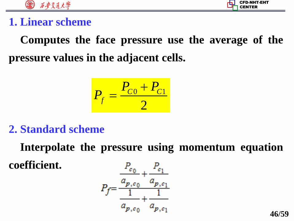
1. Linear scheme
Computes the face pressure use the average of the
pressure values in the adjacent cells.
2. Standard scheme
Interpolate the pressure using momentum equation
coefficient.
0 1
2
C Cf
P PP
47/59
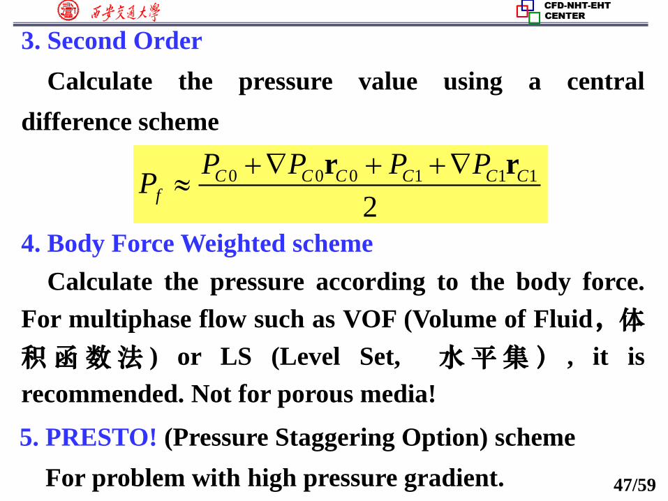
3. Second Order
Calculate the pressure value using a central
difference scheme
4. Body Force Weighted scheme
Calculate the pressure according to the body force.
For multiphase flow such as VOF (Volume of Fluid,体
积函数法 ) or LS (Level Set, 水平集) , it is
recommended. Not for porous media!
0 0 0 1 1 1
2
C C C C C Cf
P P P PP
r r
5. PRESTO! (Pressure Staggering Option) scheme
For problem with high pressure gradient.
48/59
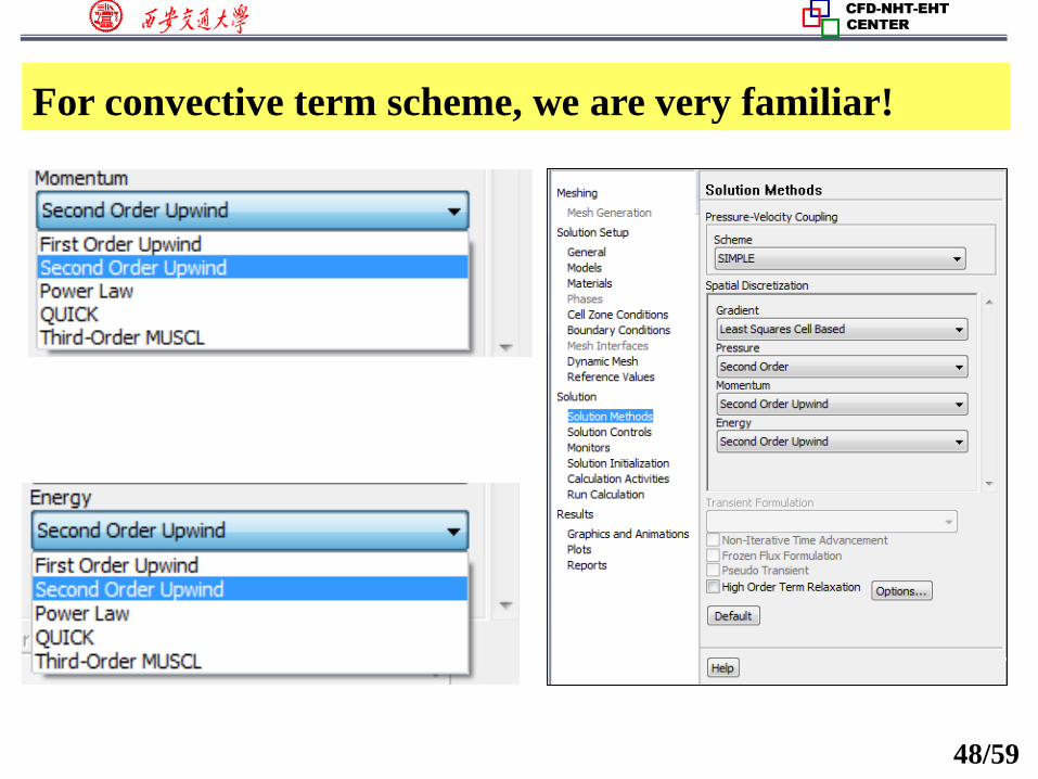
For convective term scheme, we are very familiar!
49/59
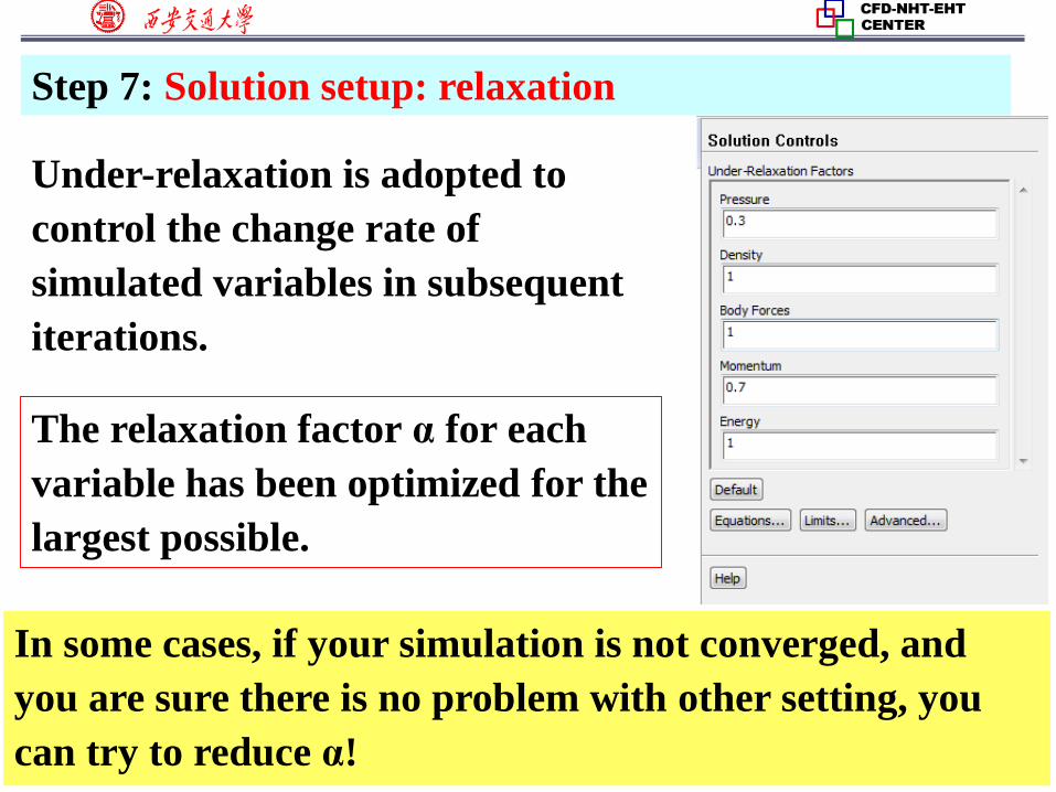
Step 7: Solution setup: relaxation
Under-relaxation is adopted to
control the change rate of
simulated variables in subsequent
iterations.
The relaxation factor α for each
variable has been optimized for the
largest possible.
In some cases, if your simulation is not converged, and
you are sure there is no problem with other setting, you
can try to reduce α!
50/59
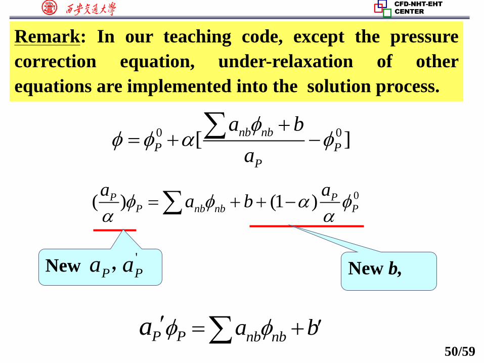
Remark: In our teaching code, except the pressure
correction equation, under-relaxation of other
equations are implemented into the solution process.
0 0[ ]nb nb
P P
P
a b
a
0( ) (1 )P PP nb nb P
a aa b
New b, New'
P Pa a,
P P nb nba ba
51/59
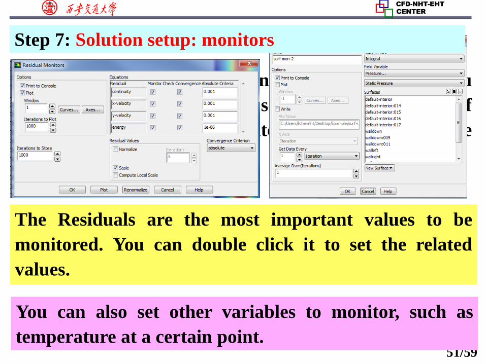
Similar to “Print” function in our teaching code, you
can use Monitors in Fluent to setup a certain number of
variables to monitor the iteration process of the
simulation.
The Residuals are the most important values to be
monitored. You can double click it to set the related
values.
You can also set other variables to monitor, such as
temperature at a certain point.
Step 7: Solution setup: monitors
52/59
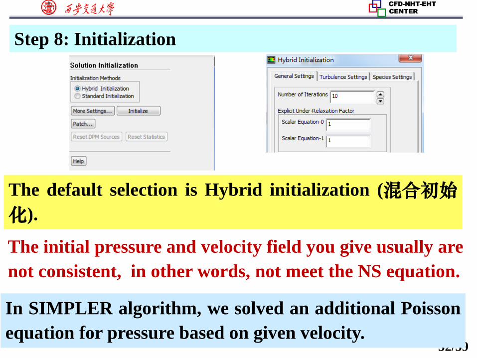
Step 8: Initialization
The default selection is Hybrid initialization (混合初始
化).
The initial pressure and velocity field you give usually are
not consistent, in other words, not meet the NS equation.
In SIMPLER algorithm, we solved an additional Poisson
equation for pressure based on given velocity.
53/59
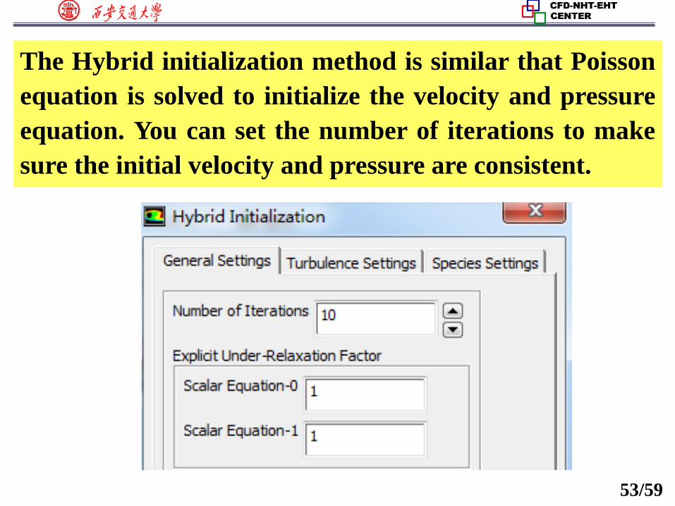
The Hybrid initialization method is similar that Poisson
equation is solved to initialize the velocity and pressure
equation. You can set the number of iterations to make
sure the initial velocity and pressure are consistent.
54/59
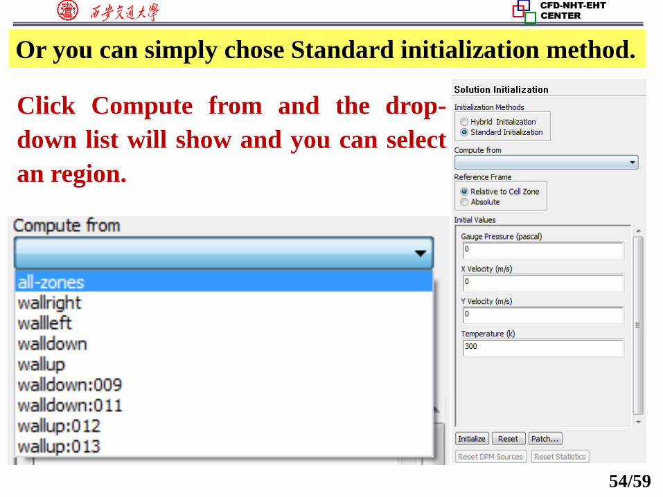
Or you can simply chose Standard initialization method.
Click Compute from and the drop-
down list will show and you can select
an region.
55/59
The eight steps for preparing a Fluent simulation have
been completed!
1. Read mesh 2. scale domain
3. Choose model 4.define material
5. define zone condition 6. define boundary condition
7. Solution step 8. Initialization
9. Run the simulation. 10. Post-process
Step 9: Run the simulation
What should you do in this step?
Just stare at the monitor to hope
that the residual curves are going
down for a steady problem.
Diverged? Go back to Steps 1 to 8.
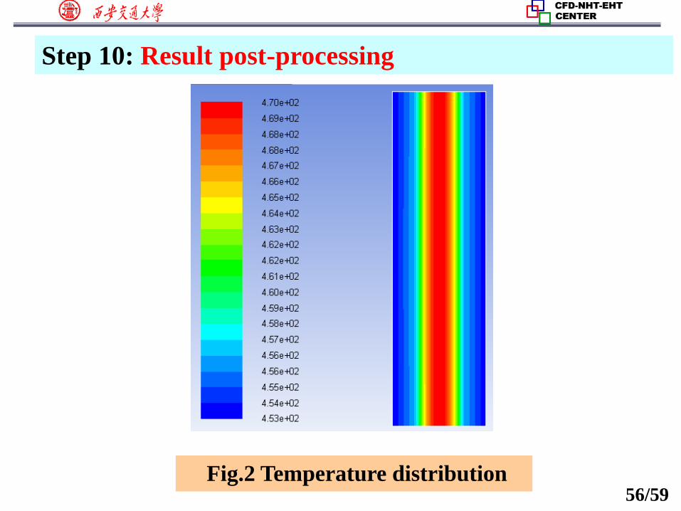
56/59Fig.2 Temperature distribution
Step 10: Result post-processing
57/59
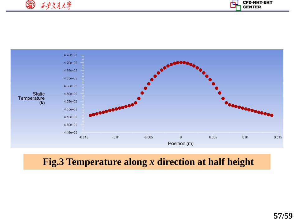
Fig.3 Temperature along x direction at half height
58/59
Review: The 10 steps for a Fluent simulation:
1. Read and check the mesh: mesh quality.
2. Scale domain: make sure the domain size is right.
3. Choose model: write down the corresponding governing
equations is very important.
4. Define material: the solid and fluid related to your problem.
5. Define zone condition: material of each zone and source term
6. Define boundary condition: very important
7. Solution step: algorithm and scheme. Have a background of
NHT.
8. Initialization: initial condition
9. Run the simulation: monitor the residual curves and certain
variable.
10. Post-process: analyze the results.
59/59
2: Operating the Fluent software to simulate the
example and post-process the results. (运行软件)
Uranium: density: 19090 kg/m3; Cp: 116 J/(kg.K)
Thermal conductivity: 27.4 W/(m.K)

1/45
Instructor Wen-Quan Tao; Qinlong Ren; Li Chen
CFD-NHT-EHT Center
Key Laboratory of Thermo-Fluid Science & Engineering
Xi’an Jiaotong University
Xi’an, 2018-Dec.-17
Numerical Heat Transfer
Chapter 13 Application examples of fluent for basic flow and heat transfer problem
2/45
数值传热学第 13 章 求解流动换热问题的Fluent软件基础应用举例
主讲 陶文铨
西安交通大学能源与动力工程学院热流科学与工程教育部重点实验室
2018年12月17日, 西安
辅讲 任秦龙,陈 黎
3/45
13.2 Unsteady cooling process of a steel ball
13.3 Lid-driven flow and heat transfer
13.5 Flow and heat transfer in chip cooling
13.1 Heat transfer with source term
13.4 Flow and heat transfer in a micro-channel
Chapter 13 Application examples of fluent for basic flow and heat transfer problem
13.6 Phase change material melting with fins
4/45
第 13 章 求解流动换热问题的Fluent软件应用举例
13.2 非稳态圆球冷却问题
13.3 顶盖驱动流动换热问题
13.5 芯片冷却流动换热问题
13.1 有内热源的导热问题
13.4 微通道内流动换热问题
导热问题
混合对流问题
微通道问题
13.6 肋片强化相变材料融化 相变传热
Review: The 10 steps for a Fluent simulation:
1. Read and check the mesh: mesh quality.
2. Scale domain: make sure the domain size is right.
3. Choose model: write down the corresponding governing
equations is very important.
4. Define material: the solid and fluid related to your problem.
5. Define zone condition: material of each zone and source term
6. Define boundary condition: very important
7. Solution step: algorithm and scheme. Have a background of
NHT.
8. Initialization: initial condition
9. Run the simulation: monitor the residual curves and certain
variable.
10. Post-process: analyze the results.
6/45
Focus: compared with previous example, this
example focuses on setting of unsteady problem.
13.2 Unsteady cooling process of a steel ball
非稳态圆球冷却问题
7/45
13.2 Unsteady cooling process of a steel ball
Known:
A steel ball with initial uniform temperature of 723 K
was placed in air of 303K.
(D=5 cm, density is 7735kg/m3, capacity is 480 J/(kg K),
conductivity is 33W/(m K) ).
Outside boundary condition : convective BC
Fluid temperature: 303K
Heat transfer coefficient: h=24W/(m2K) .
Inside :initial temperature is 723K .
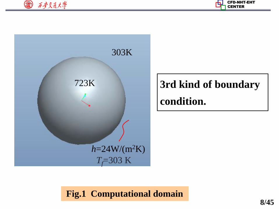
8/45
723K
303K
h=24W/(m2K)
3rd kind of boundary
condition.
Fig.1 Computational domain
Tf=303 K
9/45
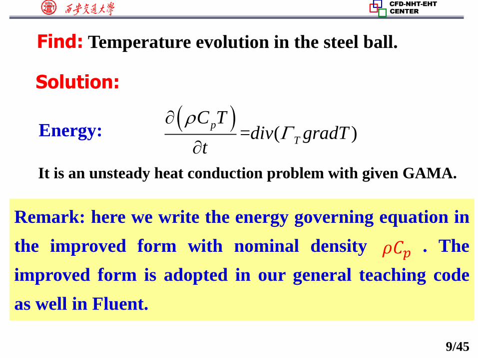
Find: Temperature evolution in the steel ball.
Solution:
Energy:
= ( )T
pdiv g
C T
tradT
It is an unsteady heat conduction problem with given GAMA.
Remark: here we write the energy governing equation in
the improved form with nominal density . The
improved form is adopted in our general teaching code
as well in Fluent.
𝜌𝐶𝑝
10/45
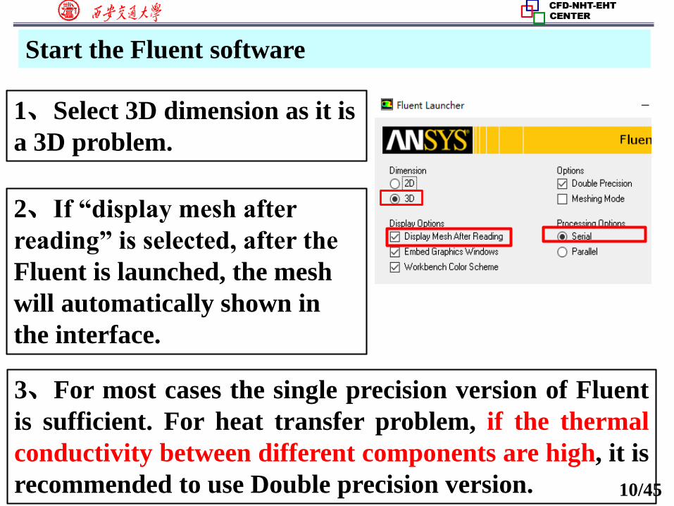
Start the Fluent software
1、Select 3D dimension as it is
a 3D problem.
2、If “display mesh after
reading” is selected, after the
Fluent is launched, the mesh
will automatically shown in
the interface.
3、For most cases the single precision version of Fluent
is sufficient. For heat transfer problem, if the thermal
conductivity between different components are high, it is
recommended to use Double precision version.
11/45
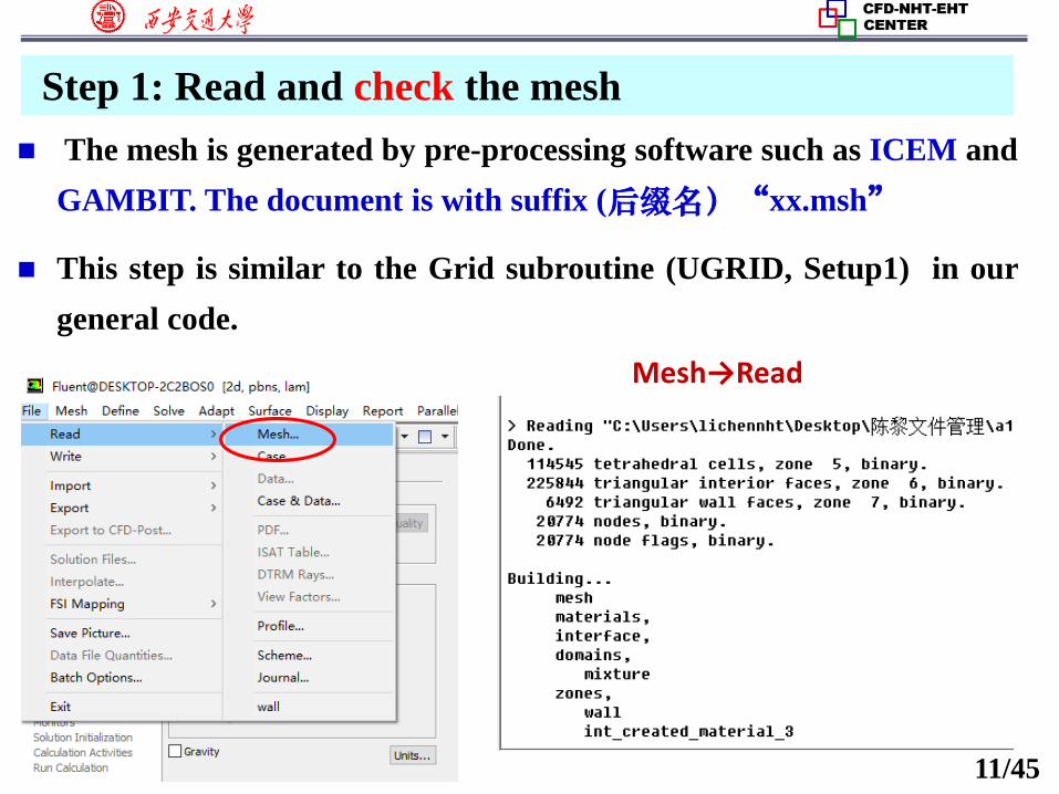
The mesh is generated by pre-processing software such as ICEM and
GAMBIT. The document is with suffix (后缀名)“xx.msh”
This step is similar to the Grid subroutine (UGRID, Setup1) in our
general code.
Mesh→Read
Step 1: Read and check the mesh
12/45
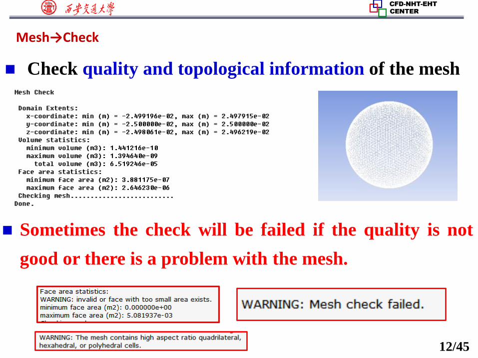
Mesh→Check
Check quality and topological information of the mesh
Sometimes the check will be failed if the quality is not
good or there is a problem with the mesh.
13/45
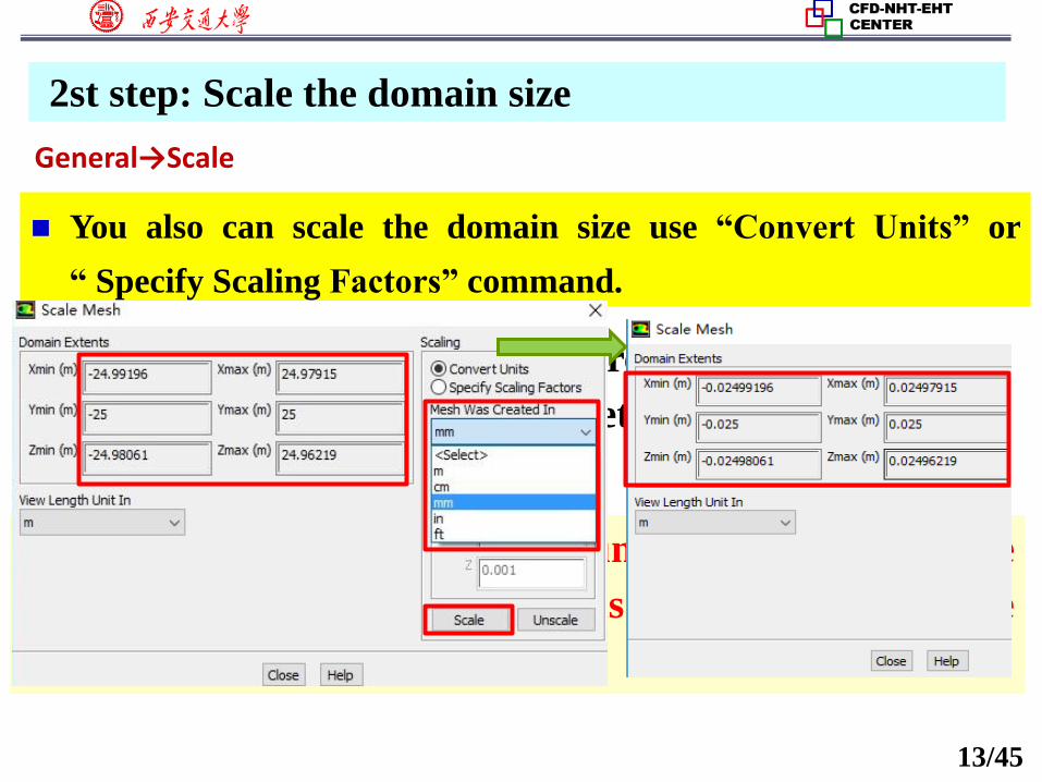
2st step: Scale the domain size
General→Scale
You also can scale the domain size use “Convert Units” or
“ Specify Scaling Factors” command.
In Example 2, the mesh was created in ICEM in the
length unit of “mm”. The diameter of the steel ball is
50mm.
Fluent import the mesh in the unit of m. Therefore, the
imported diameter is 50m which is wrong. Therefore, the
length must be scaled.
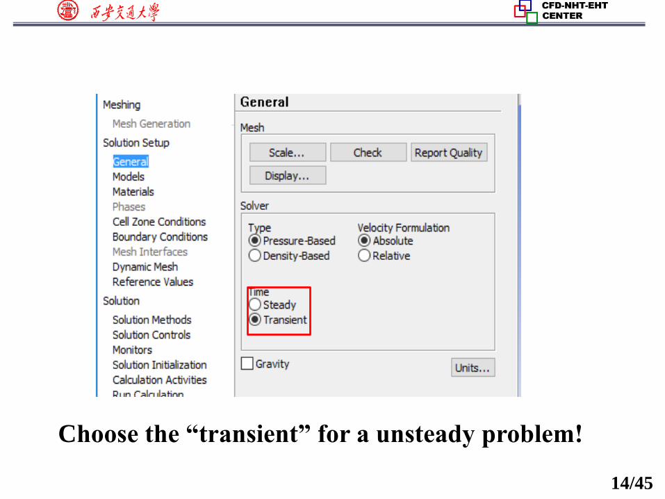
14/45
Choose the “transient” for a unsteady problem!
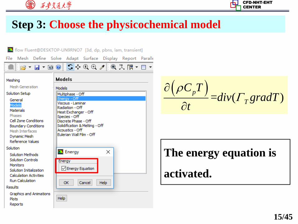
15/45
The energy equation is
activated.
Step 3: Choose the physicochemical model
= ( )T
pdiv g
C T
tradT
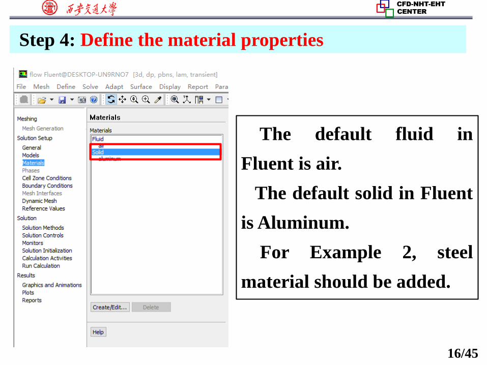
16/45
The default fluid in
Fluent is air.
The default solid in Fluent
is Aluminum.
For Example 2, steel
material should be added.
Step 4: Define the material properties
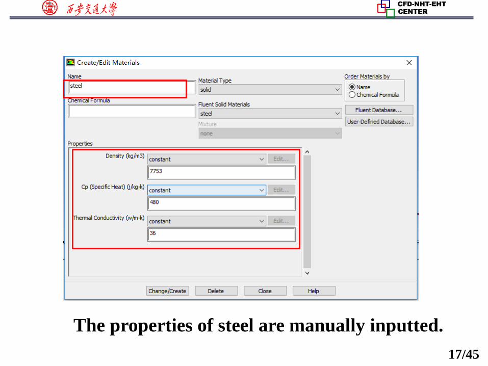
17/45
The properties of steel are manually inputted.
18/45
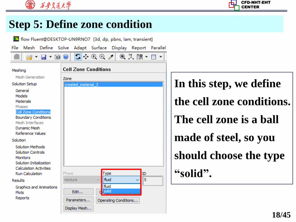
In this step, we define
the cell zone conditions.
The cell zone is a ball
made of steel, so you
should choose the type
“solid”.
Step 5: Define zone condition
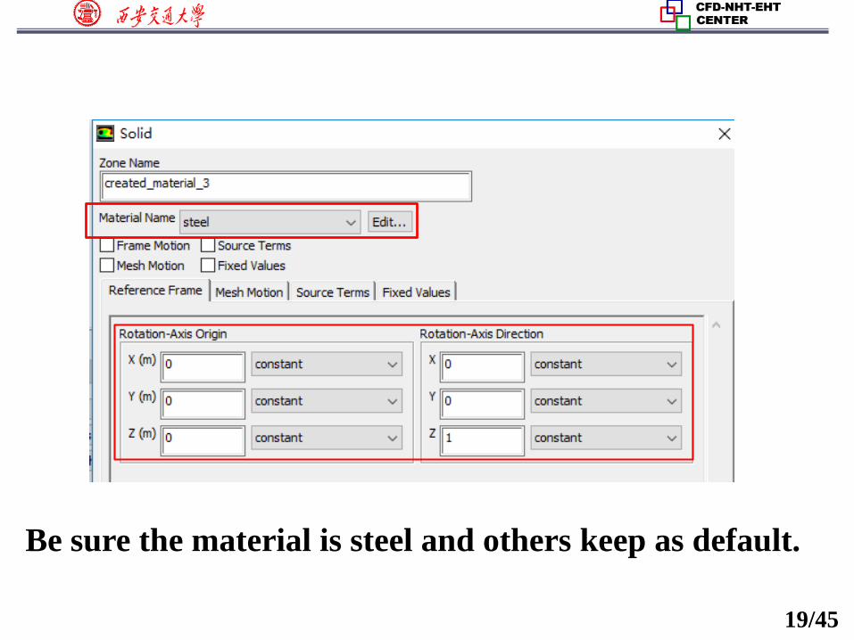
19/45
Be sure the material is steel and others keep as default.
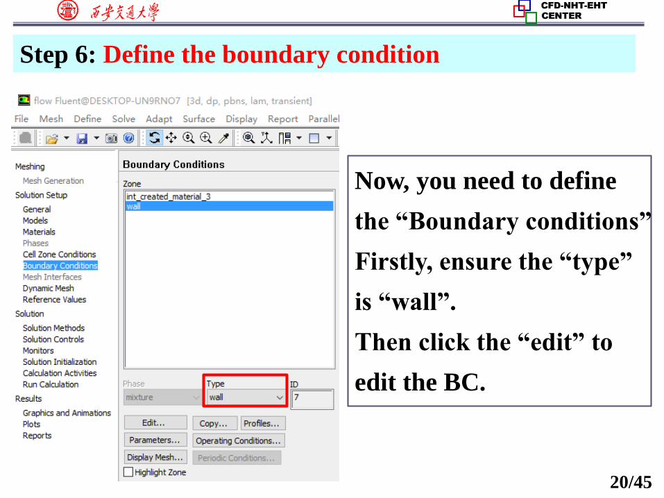
20/45
Now, you need to define
the “Boundary conditions”
Firstly, ensure the “type”
is “wall”.
Then click the “edit” to
edit the BC.
Step 6: Define the boundary condition
21/45
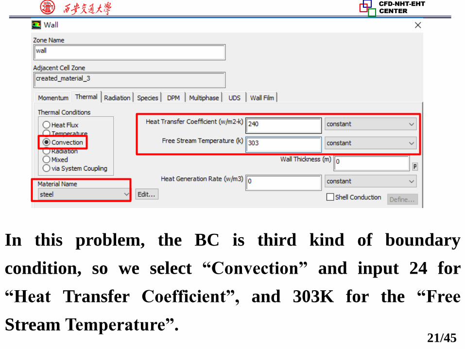
In this problem, the BC is third kind of boundary
condition, so we select “Convection” and input 24 for
“Heat Transfer Coefficient”, and 303K for the “Free
Stream Temperature”.
22/45
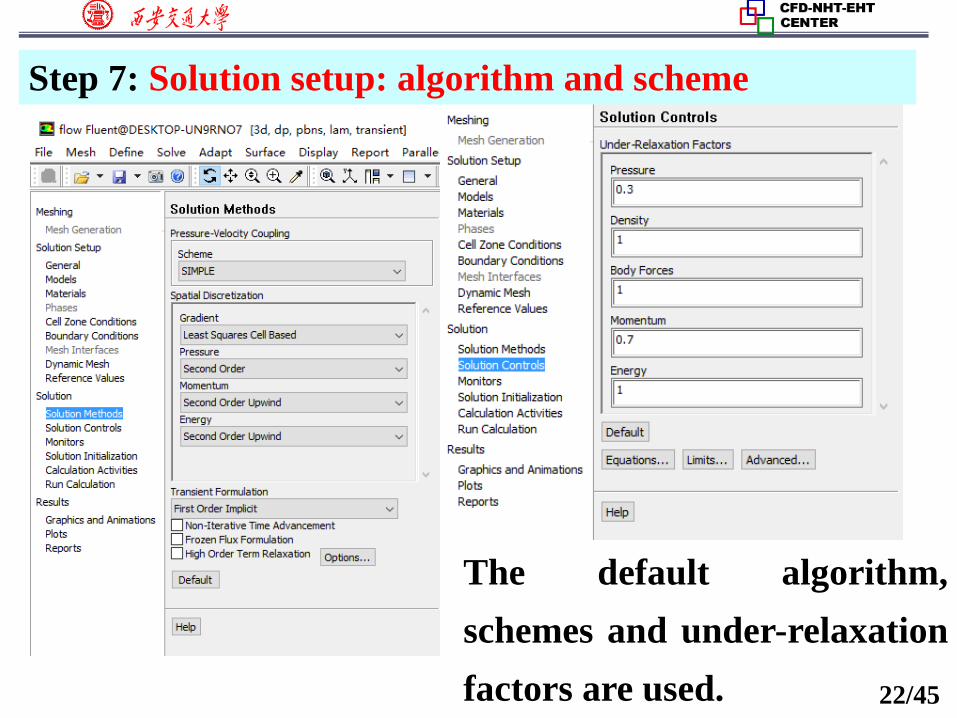
The default algorithm,
schemes and under-relaxation
factors are used.
Step 7: Solution setup: algorithm and scheme
23/45
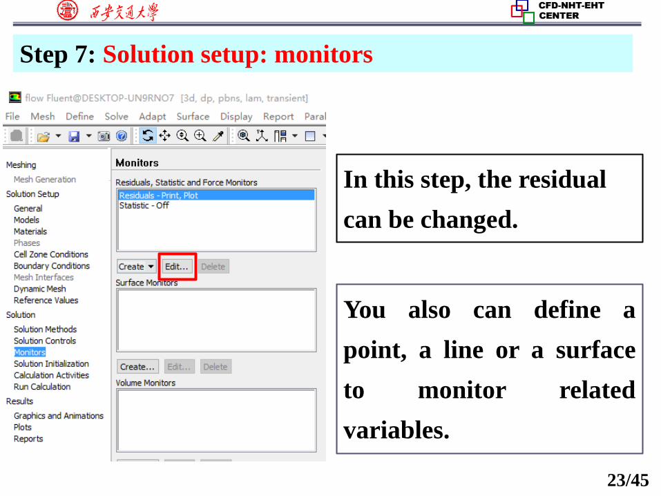
In this step, the residual
can be changed.
Step 7: Solution setup: monitors
You also can define a
point, a line or a surface
to monitor related
variables.
24/45
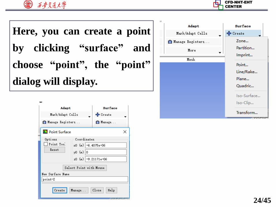
Here, you can create a point
by clicking “surface” and
choose “point”, the “point”
dialog will display.
25/45
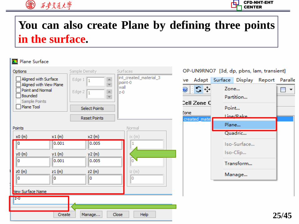
You can also create Plane by defining three points
in the surface.
26/45
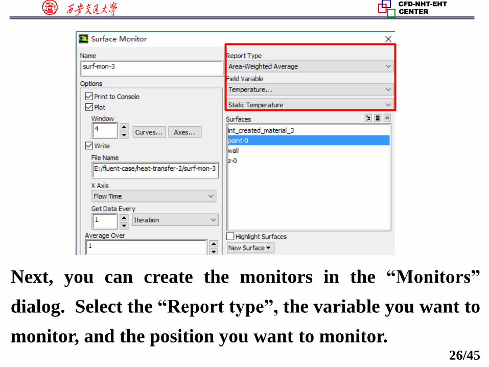
Next, you can create the monitors in the “Monitors”
dialog. Select the “Report type”, the variable you want to
monitor, and the position you want to monitor.
27/45
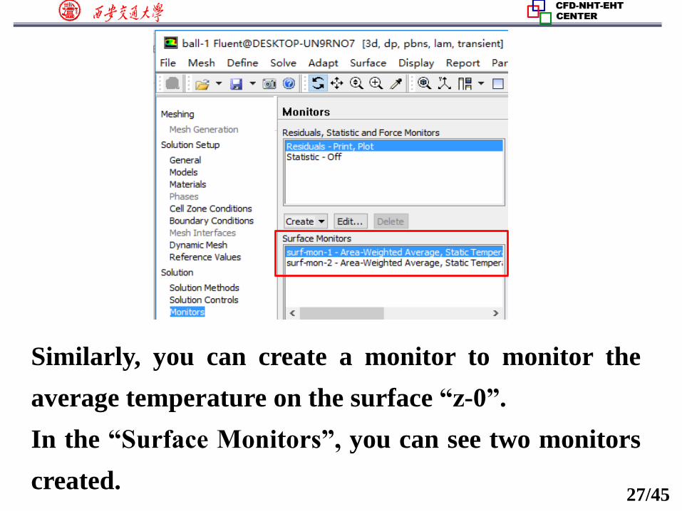
Similarly, you can create a monitor to monitor the
average temperature on the surface “z-0”.
In the “Surface Monitors”, you can see two monitors
created.
28/45
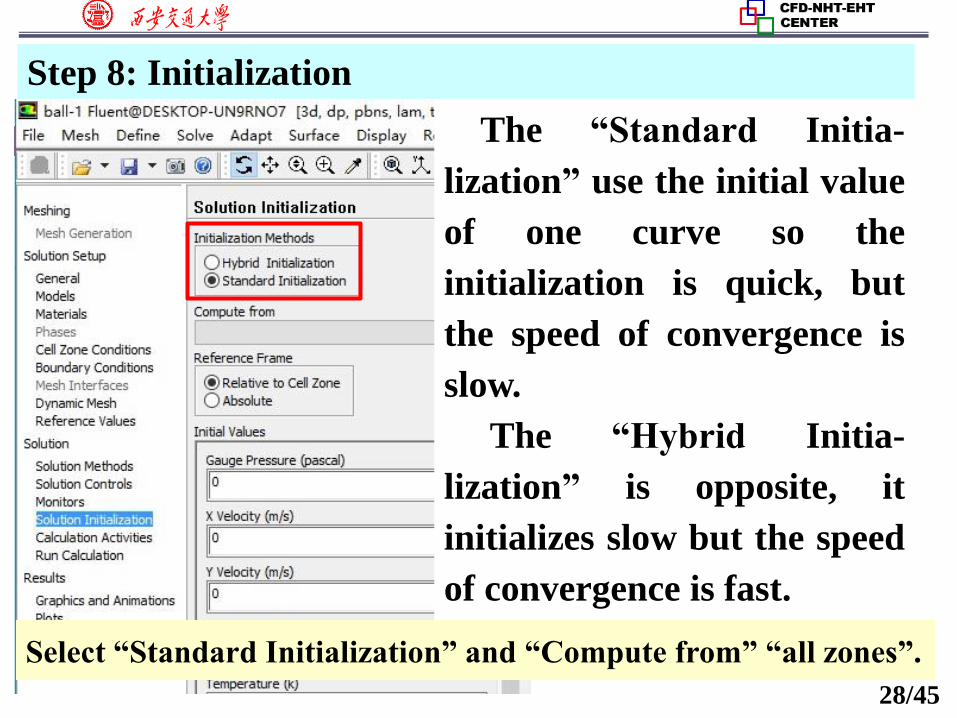
The “Standard Initia-
lization” use the initial value
of one curve so the
initialization is quick, but
the speed of convergence is
slow.
The “Hybrid Initia-
lization” is opposite, it
initializes slow but the speed
of convergence is fast.
Select “Standard Initialization” and “Compute from” “all zones”.
Step 8: Initialization
29/45
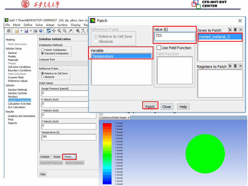
Patching (修补)Values in Selected Cells
After you have initialized the entire domain, you may
want to define a different value for a sub-region in the
domain.
For multiphase flow, you may also want to define the
volume of fraction for a phase in a particular sub-region.
This can be achieved by using the Patch function!
In Example 2, the Patch function is adopted to define
the temperature of the entire domain as 723K.
30/45
31/45
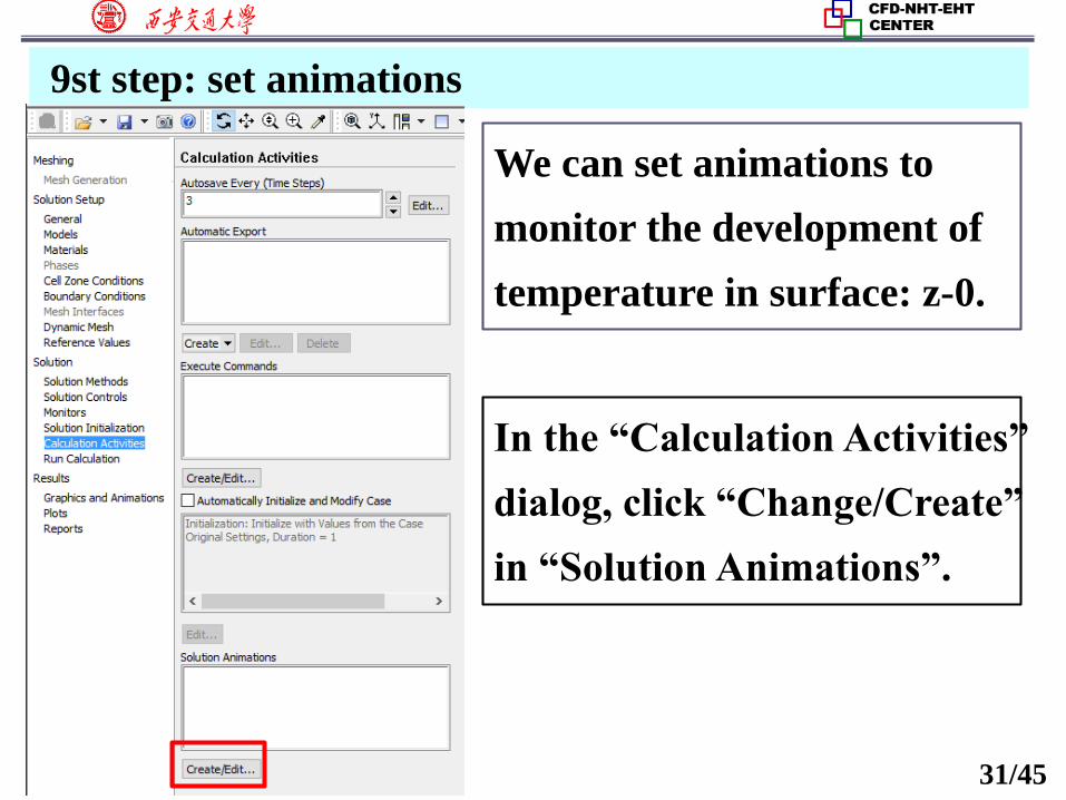
9st step: set animations
We can set animations to
monitor the development of
temperature in surface: z-0.
In the “Calculation Activities”
dialog, click “Change/Create”
in “Solution Animations”.
32/45
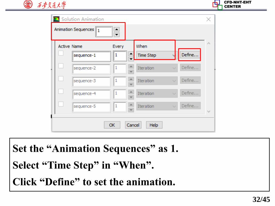
Set the “Animation Sequences” as 1.
Select “Time Step” in “When”.
Click “Define” to set the animation.
33/45
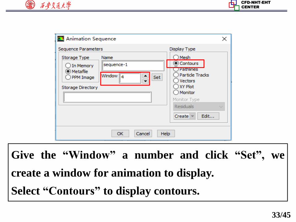
Give the “Window” a number and click “Set”, we
create a window for animation to display.
Select “Contours” to display contours.
34/45
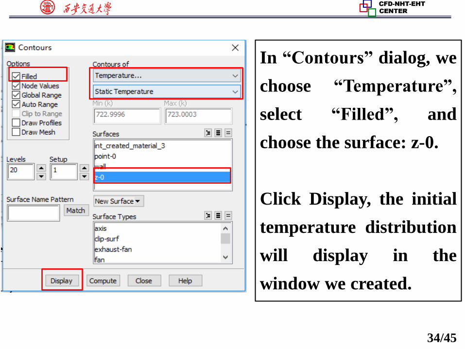
In “Contours” dialog, we
choose “Temperature”,
select “Filled”, and
choose the surface: z-0.
Click Display, the initial
temperature distribution
will display in the
window we created.
35/45
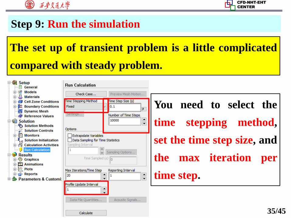
The set up of transient problem is a little complicated
compared with steady problem.
Step 9: Run the simulation
You need to select the
time stepping method,
set the time step size, and
the max iteration per
time step.
36/45
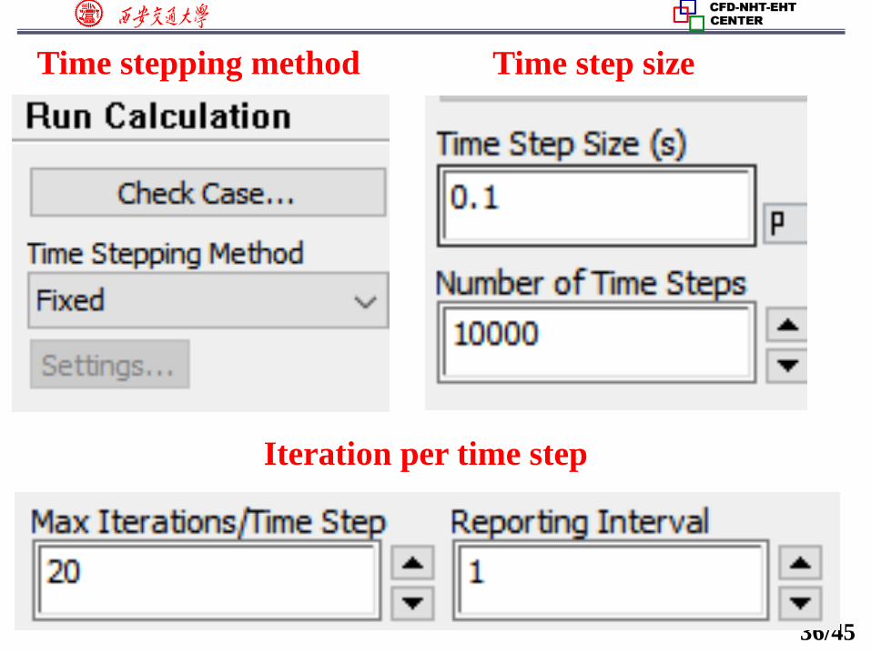
Time stepping method Time step size
Iteration per time step
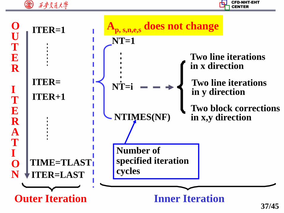
37/45
ITER=LAST
OUTER
ITERATION
ITER=1
ITER=
ITER+1
TIME=TLAST
Outer Iteration
外
迭
代
ITER=1
层 次
NF=1
NTIMES(NF)
X,Y方 向 两 次 块 修 正
X方 向 两 次 线 迭 代
Y方 向 两 次 线 迭 代
内 迭 代
ITER= LAST
外 迭 代 内 迭 代
(IT=ITER+1) 轮 次( T= T+ DT)
T= ......
NT=1
NTIMES(NF)Two block correctionsin x,y direction
Two line iterationsin x direction
Two line iterationsin y direction
外
迭
代
ITER=1
层 次
NF=1
NTIMES(NF)
X,Y方 向 两 次 块 修 正
X方 向 两 次 线 迭 代
Y方 向 两 次 线 迭 代
内 迭 代
ITER= LAST
外 迭 代 内 迭 代
(IT=ITER+1) 轮 次( T= T+ DT)
T= ......
Inner Iteration
Number ofspecified iterationcycles
NT=i
Ap, s,n,e,s does not change
38/45
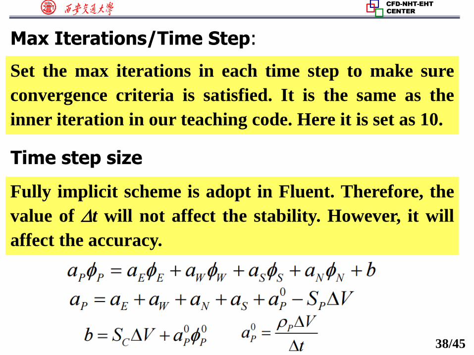
Max Iterations/Time Step:
Set the max iterations in each time step to make sure
convergence criteria is satisfied. It is the same as the
inner iteration in our teaching code. Here it is set as 10.
Time step size
Fully implicit scheme is adopt in Fluent. Therefore, the
value of t will not affect the stability. However, it will
affect the accuracy.
39/45
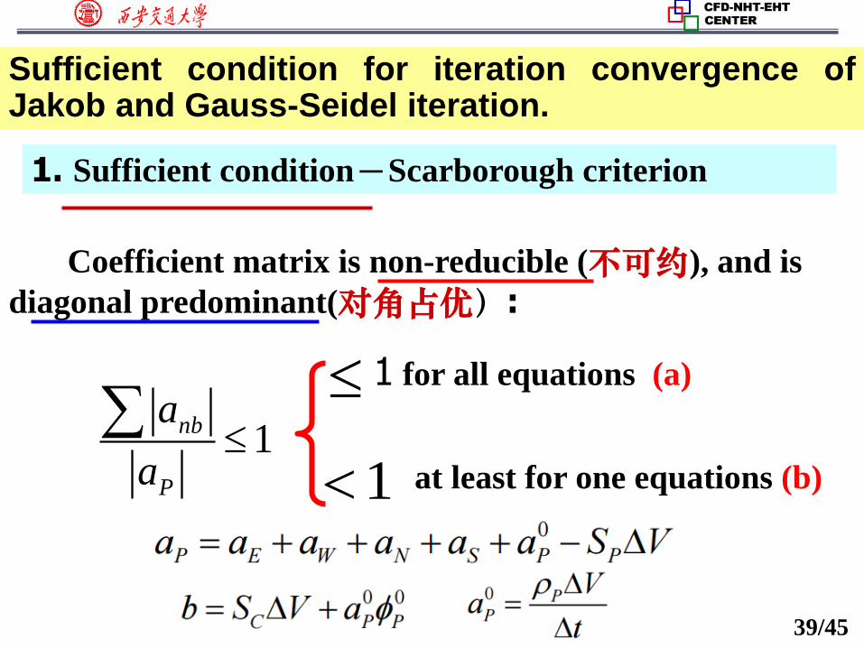
Sufficient condition for iteration convergence ofJakob and Gauss-Seidel iteration.
Coefficient matrix is non-reducible (不可约), and is
diagonal predominant(对角占优):
1. Sufficient condition-Scarborough criterion
1nb
P
a
a
1 for all equations (a)
at least for one equations (b)1
40/45
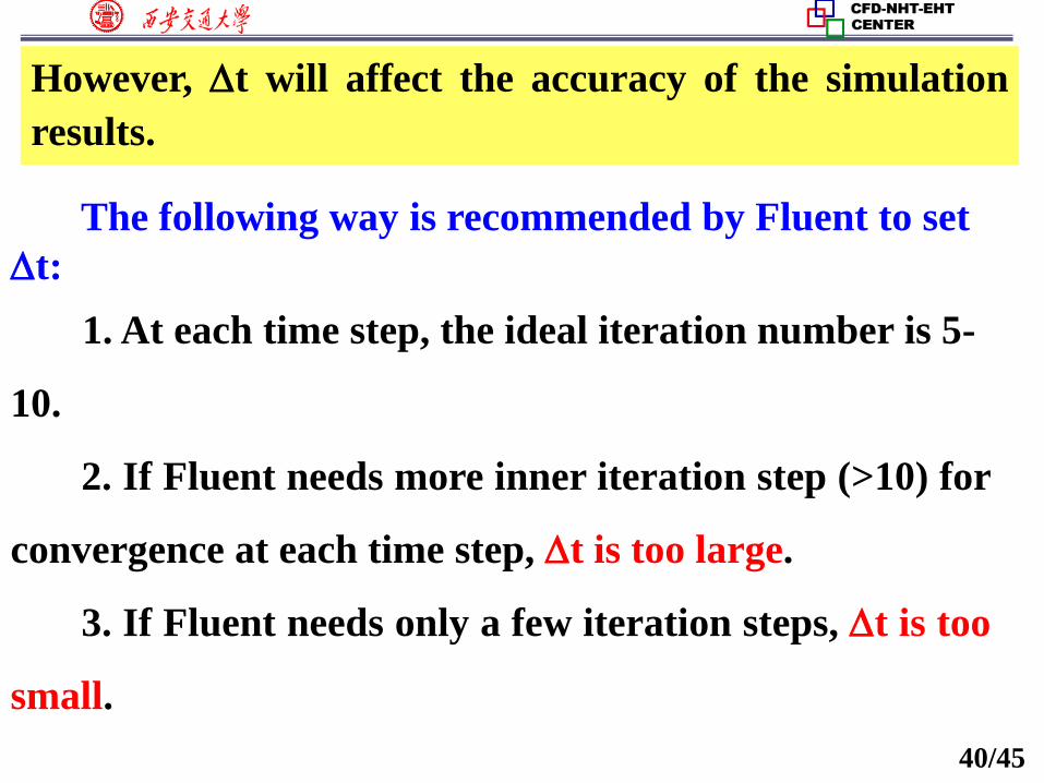
However, t will affect the accuracy of the simulation
results.
The following way is recommended by Fluent to set
t:
1. At each time step, the ideal iteration number is 5-
10.
2. If Fluent needs more inner iteration step (>10) for
convergence at each time step, t is too large.
3. If Fluent needs only a few iteration steps, t is too
small.
41/45
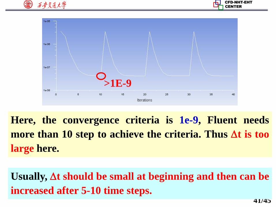
Here, the convergence criteria is 1e-9, Fluent needs
more than 10 step to achieve the criteria. Thus t is too
large here.
Usually, t should be small at beginning and then can be
increased after 5-10 time steps.
>1E-9
42/45
Time stepping method
Here for Example 2, you can simply set the time
stepping method as fixed, indicating the time step size is
not changed during the iteration.
For some problem, it is reasonable to chose Adaptive
method in which t is dynamically changed. For
example, in multiphase flow simulation using VOF, you
can use this function to update the phase interface more
efficiently.

43/45
Run the simulation
44/45
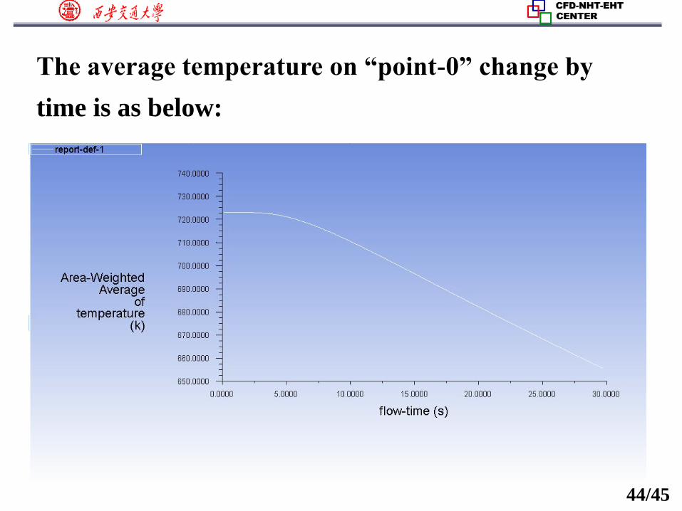
The average temperature on “point-0” change by
time is as below:
45/45
2: Operating the Fluent software to simulate the
example and post-process the results. (运行软件)
Steel: density: 7753 kg/m3; Cp: 480J/(kg.K)
Thermal conductivity: 33W/(m.K)

45/45
同舟共济渡彼岸!
People in the same boat help each other to cross to the other bank, where….