AN OPTIMIZATION MODEL: MINIMIZING FLOUR MILLERS’ COSTS …

AN OPTIMIZATION MODEL: MINIMIZING FLOUR MILLERS’ COSTS OF PRODUCTION

BY BLENDING WHEAT AND ADDITIVES

by

PHILIPPE STEFFAN

M.A., Université de Nancy II, France, 1982 M.B.A., Warwick Business School, UK, 2006

A THESIS

Submitted in partial fulfillment of the requirements

for the degree

MASTER OF AGRIBUSINESS

Department of Agricultural Economics

College of Agriculture

KANSAS STATE UNIVERSITY

Manhattan, Kansas

2012

Approved by:

Major Professor

Dr. Jason Bergtold

ABSTRACT

Grands Moulins d'Abidjan (GMA) is a flour milling company operating in Côte d'Ivoire. It

wishes to determine the optimal blend of wheat and additives that minimizes its costs of

production while meeting its quality specifications. Currently, the chief miller selects the

mix of ingredients. The management of the company would like to dispose of a scientific

tool that challenges the decisions of the chief miller.

The thesis is about building and testing this tool, an optimization model.

GMA blends up to six ingredients into flour: soft wheat, hard wheat, gluten, ascorbic acid

and two types of enzyme mixes. Quality specifications are summarized into four flour

characteristics: protein content, falling number, Alveograph W and specific volume of a

baguette after four hours of fermentation. GMA blending problem is transformed into a set

of equations. The relationships between ingredients and quality parameters are determined

with reference to grains science and with the help of linear regression.

The optimization model is implemented in Microsoft Office Excel 2010, in two versions. In

the first one (LP for Linear Programming model), it is assumed that weights of additives

can take any value. In the second one (ILP for Integer Linear Programming model), some

technical constraints restrain the set of values that weights of additives can take.

The two models are tested with Premium Solver V11.5 from Frontline Systems Inc.,

against four situations that actually occurred at GMA in 2011 and 2012,.

The solutions provided by the model are sensible. They challenge the ones that were

actually implemented. They may have helped GMA save money.

The optimization model can nevertheless be improved. The choice of relevant quality

parameters can be questioned. Equations that link ingredients and quality parameters, and

particularly those determined with the help of linear regression, should be further

researched. The optimization model should also take into account some hidden constraints

such as logistics that actually influence the decision of GMA chief miller. Finally,

sensitivity analyses may also be used to provide alternative solutions.

iv

TABLE OF CONTENTS

List of Figures ........................................................................................................................ vii

List of Tables ........................................................................................................................ viii

Acknowledgments ................................................................................................................... x

Chapter I: Introduction ......................................................................................................... 1

1.1 Thesis objective ............................................................................................................ 1

1.2 Limitations .................................................................................................................... 4

1.3 Framework .................................................................................................................... 5

CHAPTER II: LITERATURE REVIEW ........................................................................... 6

CHAPTER III: DATA AND METHODS 1 MATHEMATICAL ANALYSIS .............. 8

3.1 Optimization of wheat and additives blending ............................................................ 8

3.1.1 The Decision Variables ....................................................................................... 8 3.1.2 The Objective Function ....................................................................................... 9 3.1.3 The Constraints ................................................................................................... 9 3.1.4 Linearity ............................................................................................................ 10

3.2 Decision variables: ingredients of the mix, wheat and additives .............................. 11

3.2.1 Soft wheat .......................................................................................................... 11 3.2.2 Hard wheat ........................................................................................................ 12 3.2.3 Gluten ................................................................................................................ 13 3.2.4 Ascorbic acid ..................................................................................................... 13 3.2.5 Enzyme mixes ................................................................................................... 14

3.3 Technical constraints .................................................................................................. 14

3.3.1 GMA milling process and the incorporation of ingredients ............................ 15 3.3.2 Incorporation of wheat ...................................................................................... 16 3.3.3 Incorporation of additives ................................................................................. 17

3.4 Quality constraints: selection ..................................................................................... 20

3.4.1 Previous literature ............................................................................................. 21 3.4.2 Econometrics ..................................................................................................... 23 3.4.3 Quality constraints selection ............................................................................. 24

3.5 Quality constraints: specifications (RHS) ................................................................. 25

3.5.1 Flour protein content ......................................................................................... 25 3.5.2 Flour falling number ......................................................................................... 26 3.5.3 Alveograph W ................................................................................................... 27 3.5.4 Specific volume of baguette after 4 hours of fermentation .............................. 29

v

3.6 Quality constraints: equations (LHS) ........................................................................ 32

3.6.1 Flour protein content ......................................................................................... 33 3.6.2 Flour falling number ......................................................................................... 35 3.6.3 Alveograph W ................................................................................................... 38 3.6.4 Specific volume of baguette after 4 hours of fermentation .............................. 41

3.7 The optimization model ............................................................................................. 44

3.7.1 The Objective Function ..................................................................................... 44 3.7.2 Self-binding constraints .................................................................................... 45 3.7.3 Technical constraints ......................................................................................... 45 3.7.4 Quality constraints ............................................................................................ 45

CHAPTER IV: DATA AND METHODS COMPUTER IMPLEMENTATION ........ 47

4.1 Solver .......................................................................................................................... 47

4.2 Models ........................................................................................................................ 48

4.2.1 The LP Model ................................................................................................... 49 4.2.3 The ILP model ................................................................................................... 53

CHAPTER V: RESULTS .................................................................................................... 57

5.1 Results ......................................................................................................................... 57

5.2 Discussion ................................................................................................................... 62

5.2.1 Different optimization model solutions: LP vs. ILP ........................................ 62 5.2.2 Optimization model solutions vs. actual blends ............................................... 64

5.3 Optimization model quality constraints equations. ................................................... 70

5.3.1 Test of quality constraint equations .................................................................. 70 5.3.2 Actual flour and quality specifications ............................................................. 74

CHAPTER VI :SUMMARY AND CONCLUSIONS ...................................................... 76

Appendix A: Analysis of redundancy (correlation) of quality parameters ................... 80

Appendix B: Quality tests on different blends of wheat and additives .......................... 82

Appendix C: Test of Equation FPC1 on flours made of wheat and gluten only .......... 84

Appendix D: Test of Equation FPC1 on flours made of wheat and additives .............. 85

Appendix E: Test of Equation LNR1 on flours made of wheat only ............................. 87

Appendix F: Test of Equation LNR1 on flours made of wheat and additives .............. 88

Appendix G: Test of Equation LNR2 ................................................................................. 90

Appendix H: Test of Equation ALW1 on flours made of wheat only ............................ 92

Appendix I: Test of Equation ALW1 on flours made of wheat and additives .............. 93

Appendix J: Test of Equation ALW2 ................................................................................. 95

vi

Appendix K: Test of Equation BVL1 ................................................................................. 97

Appendix L: Test of Equation BVL2 ................................................................................. 99

Appendix M: Quality tests of actual flours ..................................................................... 101

vii

LIST OF FIGURES

Figure 1.1: GMA Logo ........................................................................................................... 1

Figure 1.2: Baguettes at GMA test bakery .......................................................................... 2

Figure 1.3: General view of GMA silos and flour mill ....................................................... 4

Figure 3.1: Ship unloading wheat at GMA facilities ........................................................ 15

Figure 3.2: GMA dosing scales............................................................................................ 16

Figure 3.3: Flour Protein Content test ............................................................................... 26

Figure 3.4: Falling Number test .......................................................................................... 27

Figure 3.5: Example of Alveograph curve ......................................................................... 28

Figure 3.6: Volumeter test ................................................................................................... 30

Figure 3.7: Weighing baguettes........................................................................................... 31

Figure 4.1: LP optimization model on Excel ..................................................................... 49

Figure 4.2: LP Premium Solver V11.5 Parameters box .................................................. 51

Figure 4.3: LP Premium Solver V11.5 Guided mode ...................................................... 52

Figure 4.4: LP Premium Solver V11.5 Options Box ........................................................ 52

Figure 4.5: ILP optimization model on Excel ................................................................... 55

Figure 4.6: ILP Premium Solver V11.5 Parameters Box ................................................ 55

Figure 4.7: ILP Premium Solver V11.5 Options Box ....................................................... 56

Figure 5.1: Premium Solver V11.5 - LP optimization model – February 2011 ............ 58

Figure 5.2: Premium Solver V11.5 - ILP optimization model – February 2011 .......... 59

Figure 5.3: Premium Solver V11.5 - ILP Answer Report – February 2011 ................. 60

Table 5.4: LP and ILP optimal solutions vs. actual ones ................................................. 61

Figure 5.4: Rounded LP optimization model – February 2011 ...................................... 63

Figure 5.5: ILP optimization model – February 2011 Answer Report .......................... 67

Figure 5.6: LP optimization model – February 2011 Sensitivity Report ....................... 69

Figure 6.1: GMA flour mill staff ......................................................................................... 76

viii

LIST OF TABLES

Table 3.1: Objective Function Formula ............................................................................... 9

Table 3.2: Constraint Formulas ............................................................................................ 9

Table 3.3: Linear Constraint Formulas ............................................................................. 11

Table 3.4: Impact of calculations on incorporation rates of additives ........................... 19

Table 3.5: Additives Weight Sets ........................................................................................ 20

Table 3.6: Quality parameters in previous literature ...................................................... 22

Table 3.7: GMA quality specifications ............................................................................... 31

Table 3.8: Regression Analyses β coefficients ................................................................... 32

Table 3.9: Equation FPC1 – Flour Protein Content ........................................................ 33

Table 3.10: Equation LNR1 – Liquefaction Number ....................................................... 35

Table 3.11: Equation LNR1 – Liquefaction Number – Soft wheat and hard wheat

only.......................................................................................................................................... 36

Table 3.12: Equation LNR2 – Liquefaction Number ....................................................... 38

Table 3.13: Equation ALW1 – Alveograph W .................................................................. 39

Table 3.14: Equation ALW1 – Alveograph W – Soft wheat and hard wheat only ...... 39



Table 3.17: Equation BVL1 – Specific Volume of Baguette ............................................ 42

Table 3.18: Equation BVL2 – Specific Volume of Baguette ............................................ 43

Table 3.19: Optimization Model – Objective Function.................................................... 44

Table 3.20: Optimization Model - Self-binding Constraints ........................................... 45

Table 3.21: Optimization Model - Technical Constraints ............................................... 45

Table 3.22: Optimization Model – Quality Constraints .................................................. 45

Table 4.1: LP/ILP model - Units Correspondence Table ................................................ 53

Table 4.2: LP/ILP model - Technical Constraints Correspondence Table ................... 53

Table 4.3: LP/ILP model - Unit Prices Correspondence Table ...................................... 54

Table 4.4: LP/ILP model – Quality Constraints Correspondence Table ...................... 54

Table 4.5: LP/ILP model – Sum of Weights Correspondence Table ............................. 54

ix

Table 5.1: Soft wheat quality parameters .......................................................................... 57

Table 5.2: Hard wheat quality parameters ....................................................................... 57

Table 5.3: Unit prices of ingredients .................................................................................. 58

Table 5.5: Rounded LP optimal solutions ......................................................................... 63

Table 5.6: Price of optimal solutions vs. actual blends .................................................... 65

Table 5.7: Quality constraints of optimal vs. actual solutions ........................................ 66

Table 5.8: Optimal solutions binding constraints and quality parameters of actual

blends ...................................................................................................................................... 67

Table 5.9: Quality parameters of actual samples of flour ............................................... 70

Table 5.10: Normal Distribution Confidence Intervals ................................................... 71

Table 5.11: Quality parameters: computed figures vs. confidence intervals ................ 72

Table 5.12: Quality parameters: computed figures vs. confidence intervals - Summary73

Table 5.13: Flour quality standards vs. actual .................................................................. 74

x

ACKNOWLEDGMENTS

The author wishes to US Wheat Associates. Messrs. Edward Wiese, Gerald Theus, James

McKenna, Peter Lloyd do a wonderful job promoting US wheat in Africa. They gave the

author the opportunity to visit the USA and to attend the flour milling short course of the

International Grains Program at Kansas State University. It was during this short course

that the author first heard about the MAB program.

The production department of Grands Moulins d'Abidjan provided all the data that made

this thesis possible. The author seizes the opportunity to thank all the staff from this

department for all the good work they do all year long.

Finally, this project would never been achieved without the support of the author's wife and

son, Julienne and Pierre.

1

CHAPTER I: INTRODUCTION

The profitability of a firm depends upon both the quality of its outputs and the costs of its

inputs. In the flour milling industry, to be profitable, a firm must produce flour that meets

the needs of its customers by choosing the correct blend of wheat and additives that is as

cheap as possible.

The second element of this statement is of particular importance. Wheat and additives

represent more than eighty percent of the total production costs of flour millers. However,

if cheap production prices result in flour of poor quality, it will have adverse effects on

operational efficiency.

Economists have designed tools that deal with such issues. Operations research and

optimization techniques simplify economic reality by using mathematical models in order

to find an optimal solution and inform decision making.

The present thesis is about the implementation of an optimization model.

1.1 Thesis objective

The objective of the thesis is to determine the optimal economic blend of wheat and

additives that minimizes flour miller’s cost of production while meeting quality

requirements. The modeling effort is based on facts and figures provided by Grands

Moulins d’Abidjan (GMA), a flour milling company operating in Côte d’Ivoire in West

Africa.

Figure 1.1: GMA Logo

2

GMA processes about 250,000 tons of wheat per year. Ninety percent of GMA flour is sold

to small bakeries, which almost exclusively produce baguettes, a French type bread. Much

smaller percentages of GMA flour are used to produce pan bread, cookies and pastries. The

present thesis will focus on bakery flour designed for making baguettes.

Figure 1.2: Baguettes at GMA test bakery

Since wheat does not grow in Côte d’Ivoire, GMA has to import it by sea vessels from

other areas of production. Quite logically, French soft wheat is well adapted to the

production of French type bread. For many years, GMA only imported French wheat in

order to produce its flour.

However, over time, in order to satisfy the needs of Ivorian bakers, as well as to keep pace

with market developments, GMA has started to blend other ingredients.

Hard wheat from North America brings higher protein content and strength to GMA flour.

Additives such as gluten, ascorbic acid or enzyme mixes modify flour characteristics. From

a technical point of view, such additives are complementary products to wheat. From an

economic point of view, hard wheat and additives can, to some extent and for some

characteristics, be considered as soft wheat substitutes. When some desired characteristics

of soft wheat are not available at hand, hard wheat or additives can be used as

replacements.

3

The specific operating conditions of GMA reinforce the importance of the issue of blending

wheat and additives.

Every year, GMA receives about 15 vessels, each of them carrying an average of 15,000

tons of soft wheat. The quality of wheat of each cargo varies from ship to ship. Due to this

variation, in order to maintain quality standards, GMA has to deal with blending problems

about every three weeks, whenever it ends up with one cargo of wheat and switches to the

next one.

GMA is located far away from wheat production areas and wheat cannot be delivered

except by sea vessels. It takes at least four weeks between the moment an order is placed

and the moment wheat is delivered to Abidjan. When the expected specifications of a cargo

are not met, GMA may ask for some refund from its suppliers, but it must nevertheless

process the wheat that has actually been received and wait several weeks for another

shipment. Unfortunately, such a problem occurs from time to time. The only solution is to

design an appropriate mix of ingredients, at short notice, to meet needed standards.

The chief miller is responsible for the blending decision. He knows the different

specifications and characteristics of ingredients, wheat and additives, in his possession. He

knows what type of flour must be produced. Capitalizing upon his experience, he designs a

satisfactory blend. This way of doing things has proved to be quite efficient over the years.

However, the management of the company believes this process can be improved.

An optimization model could help GMA define the mix of wheat and additives that both

meets the needs of its customers, while being the least expensive. The optimum defined by

this program should not replace the decision of the chief miller. However, based upon a

scientific approach, it could challenge his proposal and give rise to a hopefully fruitful

discussion before a final decision is made.

4

Figure 1.3: General view of GMA silos and flour mill

1.2 Limitations

Flour milling has to deal with blending techniques. Flour millers purchase wheat from

different geographical origins or from different classes or grades. Out of these different

inputs, they wish to produce flour of consistent quality. To do so, they use two main

techniques: blending wheat or blending flour. The two techniques have pros and cons. We

focus only on wheat blending here as GMA’s mill layout favors wheat rather than flour

blending.

It is also important to make it clear from the beginning that this study is only about

economic optimization. We will not talk about flour milling techniques. Of course, flour

millers, with the help of various processes and machines, optimize the wheat blending

process as well as the use of additives. All these techniques are beyond the scope of the

present thesis. We will focus on optimizing the blending process through economic tools

and techniques.

5

1.3 Framework

The economic optimization of wheat and additives blending is a crucial issue for flour

millers. As regards GMA, an optimization model may lead to saving significant amounts of

money. The thesis objective will be therefore to design and build a model which can

efficiently address this issue.

Another interest of the present thesis is that it provides an opportunity to apply another

technique, optimization, to a GMA business issue. As such, it fits quite adequately with the

purpose of an executive education program such as the Master of Agri-Business at Kansas

State University.

The present study is organized as follows: definition of objective; literature review; data

and methods; results and conclusion. In addition, the process takes account of the

pragmatic five-step optimization modeling process identified by Ragsdale (2008):

identifying the problem, mathematically analyzing the problem, implementing the problem

on computer, solving the problem using software tools and, finally, testing the results.

The present thesis will comprise 6 chapters. In the present Chapter 1 “Introduction”, the

thesis objective is identified and is defined. In Chapter 2, the "Literature Review" describes

previous papers or studies on similar or related subjects. It outlines how the present project

differs from these previous works. Chapter 3 "Data and Methods 1.Mathematical Analysis"

explains how actual business conditions are transformed into a set of equations and

inequalities. Chapter 4 "Data and Methods 2.Computer Implementation", depicts how the

equations of the model are captured on a spreadsheet. In Chapter 5 "Results", optimal

solutions given by the model are compared with actual decisions made by GMA. Finally,

Chapter 6 "Summary and Conclusion" draws conclusions and suggests ideas for further

research and improvement of the optimization model.

6

CHAPTER II: LITERATURE REVIEW

The objective of the present thesis is to use wheat and additives blending as a means of

minimizing flour millers’ costs of production while still meeting quality requirements.

This is a common issue among flour millers. Fowler (2009, p. 62-66) summarizes the

economic reasons why millers blend wheat and add ingredients to flour. They want to

deliver a consistent or a unique product and they want to minimize their raw material cost.

The way to achieve this objective is through optimization techniques, particularly linear

programming. Blending problems are traditional applications of linear programming. Some

of the earliest to be addressed were the nut-mix problem (Charnes et al. 1953) and the

sausage-blending problem (Steuer 1986).

Niernberger (1973) was certainly the first to formulate and evaluate a wheat blending

model in order to maximize profit from flour milling operations. He designed a

computerized linear programming model that determined the optimum blend of different

lots of wheat and maximized profit, under several technical and economic constraints.

Niernberger’s model’s purpose is close to the objectives of the present thesis. There are

nevertheless significant differences between the two efforts. Niernberger’s objective was to

optimize the flour miller’s profit originating from all its products: patent flour, 1st clear

flour, 2nd clear flour, as well as mill feed. The objective of the present thesis is only to

minimize the cost of production of one type of flour, designed for making French type

bread, baguettes. Other differences derive from geographical contexts. Niernberger’s model

only considers types of hard winter wheat. He uses Brabender Farinograph data to build

constraints and the flour produced is designed to make pan-bread. In the present thesis,

different wheat varieties from Europe and North America are mixed. The addition of

additives that may influence the price, as well as the characteristics of flour is also

considered. Flour is used to make baguettes. Finally, Chopin Alveograph is used instead of

Brabender Farinograph.

Hayta and Cakmakli (2001) used linear programming to optimize the blending of wheat

lots. Using linear regression, they identify three criteria that characterize wheat lots and that

7

are significantly correlated with loaf volume: particle size index, dough volume and falling

number. Then they design a linear programming model that determines the most economic

wheat mix. Hayta and Cakmali focus on the selection of quality criteria rather than on the

optimization problem itself. They work on wheat and flour characteristics that are different

from those used in West Africa. In addition, they do not take account of additives.

In addition to published literature, the idea of the present thesis was triggered by two other

pieces of work.

The International Grains Program (IGP) organizes short courses for flour millers, in

association with Kansas State University. The 2006 Flour Milling short course included a

lesson on spreadsheet solutions by Bryan Shurle and Mark Fowler. Among other things,

this lesson displayed an example of a wheat blending problem worked out by Microsoft

Office Excel Solver. However, although quite realistic, this spreadsheet had to be adapted

in order to meet actual constraints and become an effective tool.

In the 2000’s, Peter Lloyd of US Wheat Associates (USW) also designed a Microsoft

Office Excel spreadsheet that helped millers determine the most profitable blends of wheat.

All millers visited by US Wheat Associates can request this spreadsheet, specifically in

Africa since Peter Lloyd is based out of Casablanca, Morocco. Millers enter in the

spreadsheet several inputs such as wheat characteristics, type of flour produced, prices of

wheat, prices of flour, operating costs, etc. They choose a specific blend of wheat and the

spreadsheet enables them to compare the characteristics of this blend with what they expect

in terms of flour quality, as well as gross margin. Solver and Goal Seek functions are used

to fine tune the wheat blend. The USW spreadsheet is more ambitious than the present

thesis project: it is designed to compute flour millers’ gross margins and not only minimize

production costs. However, it takes into account only the rheological characteristics of the

flour produced. The present thesis will also consider bread-making characteristics of flour.

As all other works, the USW model does not take account of additives.

8

CHAPTER III: DATA AND METHODS 1 MATHEMATICAL ANALYSIS

In the introductory chapter, the thesis objective was identified as the minimization of flour

millers’ production costs by blending wheat and additives, while meeting flour standards.

In the present chapter, this objective as well as GMA constraints will be analyzed and

transformed into a mathematical model to be optimized.

The optimization model and its different components: variables, equations and inequalities

will be defined in section 3.1. In the subsequent sections, the different elements of the

model will be reviewed. In section 2, the decision variables, i.e. the different ingredients of

the GMA mix will be considered. In section 3, technical constraints will be identified and

described in mathematical terms. In sections 4 to 6, quality constraints will be identified,

given limits and put into equations. Finally, the whole optimization model will be displayed

in section 7.

3.1 Optimization of wheat and additives blending

In the modeling approach, the blending problem is translated into equations and/or

inequalities. The mathematical formulation of the problem requires definition of decision

variables, objective function, and constraints.

3.1.1 The Decision Variables

Decision variables represent the choice to be made: the quantities the researcher wishes to

determine. For the GMA model, decision variables (W1, W2..., Wi) are the actual weights

of the different ingredients that are blended in order to produce flour of a desired and

consistent quality.

It must be stated from the beginning of the thesis that, since Côte d’Ivoire has adopted the

metric system, all weights are expressed in metric tons (t) or kilograms (kg). And in order

to keep things simple, it is assumed that, in the present optimization model, the total weight

of all ingredients is equal to one thousand metric tons. The price of 1,000 tons of a mix of

wheat and additives is large enough to be significant. Using weights instead of respective

proportions of ingredients in the mix, for instance, makes it easier to compute prices since

unit prices are expressed in CFA francs per metric ton. The CFA franc (FCFA) is the West

9

African Economic and Monetary Union (WAEMU) currency and is worth about 0.002 US

dollars.

As regards wheat, either hard or soft, each Wi represents a weight which is associated to

one sea vessel. This is how GMA differentiates lots of wheat. Wheat from each vessel is

consistent since cargoes are homogenized in port elevators before loading. They are

handled and stored separately in GMA silos after reception at Abidjan. Last but not least, to

each and every vessel corresponds a specific unit price of wheat.

3.1.2 The Objective Function

The objective function is a function of the decision variables that the researcher wishes to

maximize or minimize. For GMA, the objective function of the optimization model is to

minimize the cost of the blend of wheat and additives processed by the mill.

Table 3.1: Objective Function Formula

Min: ΣWiPi

where:

Wi is the weight of wheat or any additive used in the mix, the total of which amounts to one thousand metric tons ;

Pi is the price of the corresponding ingredient, expressed in CFA francs per metric ton (FCFA/t).

3.1.3 The Constraints

Constraints are other functions of the decision variables. In a world of limited resources,

they are restrictions on the solutions available to any business. Constraints can be stated

mathematically as follows:

Table 3.2: Constraint Formulas f(W1, W2, ….., Wn) ≤ α, or f(W1, W2, ….., Wn) ≥ α, or

f(W1, W2, ….., Wn) = α

where:

Wi is the weight of wheat or additive used in a mix, the total of which amounts to one thousand metric tons ;

α is the limit value of the constraint.

In order to determine the optimal mix of wheat for GMA, the chief miller has to face three

categories of constraints: constraints that bind the decision variables themselves,

10

constraints that are imposed by technical considerations and, finally, constraints that

concern the quality of flour.

There are two constraints that bind the decision variables themselves. Weights of wheat

and additives cannot be negative. And, as already mentioned above, the total weight of

wheat and additives is one thousand metric tons.

Other constraints are imposed by technical considerations. Proportions of additives in the

mix should be compatible with the dosing scales of the flour mill. Incorporation rates may

be recommended by suppliers of these ingredients. The technical constraints are considered

in section 3.3.

Sections 3.4 to 3.6 deal with quality constraints. Relevant quality constraints parameters

must be selected. Specifications must be defined for these constraints. Finally, the

mathematical functions that link the ingredients of the mix and the selected quality

constraints parameters must be identified.

3.1.4 Linearity

In principle, objective function and constraints can have any mathematical form. The

important point is that they should accurately describe the problem which is to be solved.

However, preferably, functions representing the objective function and constraints should

be linear. According to Studenmund (2006, p. 207-208), a function can be linear in the

variables and/or linear in the coefficients. A function is linear in the variables “if plotting

the function in terms of X and Y generates a straight line”. A function is linear in the

coefficients “if the coefficients appear in their simplest form – they are not raised to any

powers (other than one), are not multiplied or divided by other coefficients, and do not

themselves include some sort of function (like logs or exponents)”.

Solving a set of linear functions is easier and is more reliable than a set of non-linear

functions. When using only linear functions, operations research is often termed linear

programming (LP). In the course of the present thesis, one non-linear function will be

tested but only linear functions will eventually be used in the optimization model.

11

Table 3.3: Linear Constraint Formulas β0 + β1W1 +β2W2 + … + βnWn ≤ α, or β0 + β1W1 +β2W2 + … + βnWn ≥ α, or β0 + β1W1 +β2W2 + … + βnWn = α

where:

Wi is the weight of wheat or any additive used in a mix, the total of which amounts to one thousand metric tons ;

βi is the technical coefficient attached to Wi ;

α is the limit value of the constraint.

3.2 Decision variables: ingredients of the mix, wheat and additives

In order to make flour, GMA can mix up to six ingredients: soft wheat, hard wheat, gluten,

ascorbic acid and two types of enzyme mixes.

In further developments, flour made out of some or all of these ingredients will be

referenced to by letters ‘FLR’. For instance, the price of soft wheat will be labeled PFLR.

3.2.1 Soft wheat

Soft wheat is the main ingredient of GMA flour designed for making baguettes. The total

mix usually includes up to 90% or 95% soft wheat. Soft wheat processed by GMA is

imported mostly from France. However, GMA also exploits market opportunities and, from

time to time, imports soft wheat from other origins such as the Black Sea region, Germany

or Argentina.

GMA collects data on soft wheat for every vessel that comes to Abidjan, at various stages

of the supply process.

Samples of wheat are tested in the port of loading silos as well as later, when the ship is

unloaded in Abidjan. These analyses provide data about physical (dockage, moisture etc.)

as well as rheological (protein content, falling number, Alveograph etc.) characteristics of

every cargo of wheat.

Upon arrival, a sample of soft wheat from every vessel is also processed and transformed

into flour in GMA mills. Milling and rheological characteristics of this flour are analyzed.

It is also baked and transformed into bread and graded at the GMA test bakery.

12

Altogether, GMA can characterize every cargo of soft wheat with some twenty parameters.

The GMA accounting system computes a price for every shipment of wheat. This price is

expressed in CFA francs per ton (FCFA/t). It comprises the Cost, Insurance and Freight

(CIF) price plus all forwarding costs involved until wheat is stored in bins and ready for

milling.

In recent periods of time, the price of soft wheat has suffered from high volatility. Prices

recorded by GMA follow the fluctuations of world market prices with a few weeks delay

due to transportation time. In addition, they are affected by fluctuations in freight rates. In

January 2010, the price of soft wheat at GMA was 124,688 FCFA/t. It was relatively stable

until July 2010. Then it started to increase rapidly and went from 202,844 FCFA/t in

September 2010 to 229,343 FCFA/t in March 2011.It remained at high levels until

September 2011. Then the price went down, but it is still subject to significant fluctuations.

In March 2012, GMA price for soft wheat was 197,575 FCFA/t.

Soft wheat will be referred to by the letters ‘sw’. The weight of soft wheat in the mix of

ingredients will be labeled Wsw and the unit price of soft wheat will be labeled Psw.

3.2.2 Hard wheat

At a low incorporation rate, hard wheat, with its higher protein content, brings many

interesting properties that are appreciated by GMA customers: baking strength, tolerance,

bread volume, etc. However, high percentages of incorporation of hard wheat can have

negative effects, which do not suit the production of baguettes.

Hard wheat is imported by GMA from North America. In the past years, GMA has

imported mostly Canada Western Red Spring (CWRS) wheat. CWRS is hard red spring

wheat of superior milling and baking quality.

When GMA purchases hard wheat, it performs the same tests as on soft wheat. These tests

provide data on physical, as well as rheological characteristics of the wheat. In addition, on

every shipment, GMA processes a few kilograms of hard wheat in a laboratory mill. The

rheological, as well as milling characteristics of this flour are tested

13

However, GMA does not transform this sample of flour into bread. The weight of flour

obtained from the laboratory mill is too small. Moreover, it is well known that 100% hard

wheat flour does not fit the production of baguettes. Consequently, unlike soft wheat, GMA

does not record the baking characteristics of its hard wheat supplies.

The price of hard wheat is usually higher than the price of soft wheat. It is computed by the

GMA accounting system in exactly the same way as soft wheat. This price has also been

subject to significant fluctuations in recent periods of time. It actually ranged from 163,682

FCFA/t in November 2009 to 253,491 FCFA/T in November 2011.

Hard wheat will be referred to by the letters ‘hw’. The weight of hard wheat in the mix of

ingredients will be labeled Whw and the unit price of hard wheat will be labeled Phw.

3.2.3 Gluten

Gluten is made of water insoluble proteins, glutenins and gliadins. Gluten can be found in

wheat kernels. It is also marketed on its own.

GMA incorporates gluten in the mix whenever soft wheat lacks protein content. Gluten can

be seen as a substitute for hard wheat. However, its effects have a more limited range.

The price of gluten is linked to the price of wheat but is nevertheless more stable. GMA

recorded a price of gluten at 1,286 FCFA/kg in October 2010. It reached a peak in

September 2011 at 1,618 FCFA/kg and went down to 1,205 FCFA/kg in January 2012.

Gluten will be referred to by the letters ‘GLT’. The weight of gluten in the mix of

ingredients will be labeled WGLT and the unit price of gluten will be labeled PGLT.

3.2.4 Ascorbic acid

Ascorbic acid is incorporated into flour essentially because of its functionality properties. It

is an oxidizing agent that favors the baking process. It increases dough extensibility.

Ascorbic acid price varies significantly according to its origin. In 2011, GMA purchased

ascorbic acid from Europe at 12,186 FCFA/kg and from China at 5,246 FCFA/kg.

14

Ascorbic acid will be referred to by the letters ‘AAC’. The weight of ascorbic acid in the

mix of ingredients will be labeled WAA C and the unit price of ascorbic acid will be labeled

PAAC.

3.2.5 Enzyme mixes

There are many different kinds of enzymes that flour millers incorporate in their mixes:

amylases, proteases, lipases, glucose-oxidases, etc. These products act as catalysts. They

trigger or enhance chemical reactions during the baking process. Flour millers use enzymes

to correct wheat deficiencies and help provide for consistent quality flour.

Knowledge about the effects of these different enzymes has dramatically improved in past

years. It is very difficult for a flour miller like GMA to keep up to date with progresses

made in this domain of research. As a consequence, GMA is not able to formulate by itself

relevant enzyme mixes that can address its quality issues. GMA refers to specialized firms

that design its enzyme mixes. The formulas of these enzyme mixes are kept confidential by

the supplier and GMA does not know the composition exactly.

In 2011 and 2012, GMA used two different enzyme mixes. The price of Enzyme Mix 1

varied from 26,504 FCFA/kg in December 2010 to 27,256 FCFA/kg in February 2011.The

price of Enzyme Mix 2 is equal to 24,752 FCFA/kg and is unique since GMA has

purchased only one lot of it.

The first enzyme mix and the second enzyme mix will be referred to as ‘EN1’ and ‘EN2’,

respectively. Weights of EN1 and EN2 in the total mix of ingredients will be labeled WEN1

and WEN2, respectively. Unit prices of EN1 and EN2 will be labeled PEN1 and PEN2,

respectively.

3.3 Technical constraints

In order to find a relevant solution to the optimization problem, it is necessary to consider

the technical constraints of the mill. The milling process, the capabilities of dosing scales,

as well as suppliers’ advice have an impact on the incorporation of ingredients.

15

In the case of wheat, the relative proportions of soft and hard wheat can be affected. In the

case of additives, the set of weights that can actually be incorporated in a mix of one

thousand metric tons is restricted to certain values.

3.3.1 GMA milling process and the incorporation of ingredients

Wheat is unloaded on the quays of Abidjan harbor and is directed by conveyors to GMA

elevators.

Figure 3.1: Ship unloading wheat at GMA facilities

After a period of storage, soft wheat and hard wheat are blended in a silo bin. The blend is

then conveyed to the flour mill. It is cleaned, tempered and put to rest. Flour milling theory

teaches that soft wheat and hard wheat should be treated differently, as regards the amount

of water that is added to wheat and the time it is allowed to rest. However, for decades,

GMA has not respected these differences and is used to blending and treating soft wheat

and hard wheat together.

Afterwards, the blend of wheat goes through a series of roller mills and sifters in order to

separate endosperm from bran and to reduce endosperm particles in the flour. Flour is

collected and goes through conveyors to flour bins. Dosing scales are implemented on

these conveyors so that GMA can put additives, gluten, ascorbic acid and enzyme mixes,

into the flour.

16

Figure 3.2: GMA dosing scales

After flour has been stored in bins, it is extracted, put into bags and finally delivered to

customers.

3.3.2 Incorporation of wheat

At GMA, soft wheat and hard wheat are blended together in a silo bin. The relative

proportions of soft wheat and hard wheat that are directed to this silo bin are pre-

determined by scales which are computer-controlled. The precision of these scales is of half

a percent.

It means that in a lot of 1,000 metric tons of wheat, weights of soft wheat and hard wheat

can only be multiples of 5 tons.

However, when additives are added to the mix, respective weights of soft wheat and hard

wheat can assume other values. If, for instance, 4 tons of gluten are added into the mix, the

weight of wheat amounts to 996 tons in a total of 1,000 metric tons and 0.5% of this weight

represents 4.98 tons. If, for instance, 1 ton of gluten and 56 kilograms of enzyme mix are

added into the mix, the total weight of wheat amounts to 998.944 tons in a total of 1,000

tons and 0.5% of this weight represents 4.99472 tons.

17

Since weights of soft wheat and hard wheat can take such different values in a mix of one

thousand metric tons, it will be assumed in the optimization model that these variables are

continuous.

3.3.3 Incorporation of additives

a) Additives: Incorporation rates and increments

When it comes to additives, one has to consider both limitations and sensibilities of dosing

scales but also recommendations from suppliers of ingredients.

GMA dosing scales are able to add gluten into flour at a rate which ranges between 0.1%

and 1.0% with increments of 0.1%.

Ascorbic acid is usually added to flour at rates which can vary between 0 to 100 parts per

million (ppm). Because of GMA dosing scales capabilities, this rate of incorporation can

only increase by steps of 10 ppm.

According to its supplier, enzyme mix 1 is to be incorporated at a rate of 70 ppm. It also

recommends that enzyme mix 2 should be mixed into flour at rates of 5, 10, 15 or 20 ppm.

Incorporation rates may vary but with increments of 5 ppm and a maximum limit of 20

ppm.

The above rates and increments are computed, as is usual in a flour mill, upon the basis of

flour weights. In the optimization model, these rates and increments need to be recalculated

upon the basis of the weight of the total mix of ingredients.

b) Additives: Incorporation rates denominator

Two steps are necessary to change the denominator of incorporation rates of additives.

First, they must be computed over weights of wheat instead of weights of flour. Then, they

must be calculated over the total weight of wheat and additives instead of the weight of

wheat only.

The rate of flour extraction out of wheat depends on many different parameters ranging

from wheat characteristics: dockage, moisture, hardness etc., to the milling process: length

18

of roller mills, flour ash rate etc. It is difficult to predict precisely what an extraction rate of

flour out of wheat will be. However, GMA statistical records show that, on the long run, its

extraction rate is, on the average, equal to 80%.

Such an extraction rate may appear quite high to US millers which process hard wheat. Soft

wheat extraction rates are generally higher than hard wheat. In addition, GMA flour mills

have been designed to provide a high extraction rate.

When computed on wheat rather than flour, the above incorporation rates and increments

should therefore be multiplied by 80%. If the incorporation rate of gluten is, for instance, of

0.7% on flour, it is equal to (0.7% x 80%) = 0.56% on wheat. With this formula,

incorporation rates on flour can be transformed on incorporation rates upon the basis of the

wheat blend.

However, what is needed is incorporation rates computed on the weight of the total mix,

wheat and additives included.

If, for instance, gluten is the only additive that is incorporated in the mix, then 0.56% on

wheat is equal to 0.56 / (100 + 0.56) = 0.5569% when computed on the weight of the total mix. In

another example, 0.8% of gluten and 50ppm of ascorbic acid and 56 ppm of enzyme mix 1

are added to a basis of wheat. When calculated with reference to the weight of the total

mix, these incorporation rates become, respectively, 0.8 / (100 + 0.8 +0.005 + 0.0056) = 0.7936% of

gluten and 0.005 / (100 + 0.8 + 0.005 + 0.0056) = 49.6ppm of ascorbic acid and 0.0056 / (100 + 0.8 + 0.005 +

0.0056) = 55.5ppm of enzyme mix 1.

In the following table, all additives are incorporated at their maximum rate and the

differences between incorporation rates calculated on the mix of wheat or on the total mix

are at their maximum.

19

Table 3.4: Impact of calculations on incorporation rates of additives Incorporation

rates

computed

over weight

of flour

Incorporation

rates

computed

over weight

of wheat (A)

Weights

(metric

tons)

Weights (for a

total of 1,000

metric tons)

Incorporation rates

computed over

weight of the mix

(B)

Difference

(A-B)

Wheat 1,000.0000 991.9139

Gluten 1.0000% 0.8000 % 8.0000 7.9353 0.7935% 0.0065%

Ascorbic acid 100.0000 ppm 80.0000 ppm 0.0800 0.0794 79.3531 ppm 0.6469 ppm

Enzyme mix 1 70.0000 ppm 56.0000 ppm 0.0560 0.0555 55.5472 ppm 0.4528 ppm

Enzyme mix 2 20.0000 ppm 16.0000 ppm 0.0160 0.0159 15.8706 ppm 0.1294 ppm

TOTAL 1,008.1520 1,000.0000

The maximum relative difference on incorporation rates calculated on the weight of wheat

and incorporation rates calculated on the weight of the total mix is equal to (0.8000 – 0.7935) /

0.8000 = (80.0000 – 79.3531) / 80.0000 = (56.0000 – 55.5472) / 56.0000 = (16.0000 – 15.8706) / 16.0000 = 0.8086%.

This error term is not significant. It is below the sensitivity limits of dosing scales.

Increments defined by the manufacturers of these dosing scales are much higher than this

error term. In addition, the uncertainty implied by the use of 80% as the average extraction

rate of GMA is, by far, larger.

As a consequence, in order to simplify the model, the difference between incorporation

rates upon the basis of wheat and incorporation rates upon the basis of the total mix will be

neglected. Incorporation rates computed on the weight of wheat will be used without

change in the optimization model.

c) Additives: Weight sets

Gluten is incorporated in the mix at a rate nGLT, calculated on the weight of flour, which

ranges between 0.1% and 1.0% with increments of 0.1%. On wheat, with an extraction rate

of 80%, the set of relevant incorporation rates becomes: nGLT є{0.00%; 0.08%; 0.16%;

0.24%; 0.32%; 0.40%; 0.48%; 0.56%; 0.64%; 0.72%; 0.80%}.

Ascorbic acid is incorporated in the mix at a rate, nAAC, which ranges between 0 and 100

ppm with increments of 10 ppm, on the weight of flour. The set of relevant incorporation

20

rates on the weight of wheat is: nAAC є {0ppm; 8ppm; 16ppm; 24ppm; 32ppm; 40ppm;

48ppm; 56ppm; 64ppm; 72ppm; 80ppm }.

Supplier recommends that enzyme mix 1 is incorporated at a rate, nEN1 of 70ppm on the

weight of flour. The set of relevant incorporation rates on the weight of wheat is: nEN1 є

{0ppm; 56ppm}.

Supplier recommends that enzyme mix 2 is incorporated at a rate nEN2 between 5 and

20ppm with increments of 10ppm on the weight of flour. The set of relevant incorporation

rates on the weight of wheat is: nEN2 є {0ppm; 4ppm; 8ppm; 12ppm; 16ppm}.

Assuming that incorporation rates on wheat are not significantly different from

incorporation rates on the total mix of ingredients, they can be transformed into sets of

relevant weights for additives when the weight of the total mix is equal to 1000 tons. All

weights are expressed in metric tons.

Table 3.5: Additives Weight Sets

Gluten WGLT є{0.0; 0.8; 1.6; 2.4; 3.2; 4.0; 4.8; 5.6; 6.4; 7.2; 8.0}

Ascorbic Acid WAAC є {0.000; 0.008; 0.016; 0.024; 0.032; 0.040; 0.048; 0.056; 0.064; 0.072; 0.080}

Enzyme Mix 1 WEN1 є {0.000; 0.056}

Enzyme Mix 2 WEN2 є {0.000; 0.004; 0.008; 0.012; 0.016}

These sets of relevant weights are technical constraints of the optimization model. They

have a significant impact on the optimization model since they change the model from a

Linear Programming (LP) model to an Integer Linear Programming (ILP) model.

3.4 Quality constraints: selection

GMA is very concerned about the quality of its products. It records many different data

about its flour quality: physical, rheological, milling characteristics as well as baking

characteristics. Altogether, GMA can display at least twenty series of data about each lot of

flour manufactured.

It is not desirable however to build twenty constraints in an optimization model. The

higher the number of constraints, the more time and IT resources consuming the

21

optimization model is. Some of these constraints may be irrelevant or redundant. In

addition, with too many constraints, a feasible solution may become difficult to find. The

model is more robust when it has only a few constraints.

In order to select relevant quality constraints, two types of references will be used: previous

literature and econometrics.

3.4.1 Previous literature

The parameters that were selected as constraints in previous literature are not the same

from one work to another.

Niernberger (1973) used 9 characteristics as quality constraints. The IGP model is based

upon 4 constraints. The US Wheat Associates model uses 8 constraints. In these different

works, the way quality constraints were selected is not explicit. On the other hand, Hayta

and Cakmali (2001) use econometrics techniques to select 3 constraints that are highly

correlated to loaf volume of bread.

The following table summarizes the parameters that were selected as constraints in these

works.

22

Table 3.6: Quality parameters in previous literature Niernberger

(1973) IGP model US Wheat

Associates model

Hayta & Cakmali (2001)

Physical Wheat Traits

Test Weight X

Moisture X

Wheat protein X

Falling number X X

Milling and Rheological Traits

Wet Gluten X X

Flour protein X X

Alveo P X

Alveo L X

Alveo W X

Alveo P/L X

Flour ash X X

Particle Size Index X

Far. Absorption X

Far. Arrival time X

Far. Development time X

Far. Valorimeter X

Starch Damage X

Baking Data

Dough volume X

Loaf volume X

Total score X

No single quality parameter has been selected by more than two authors. Only four of them

have been selected by two authors: Falling number, Wet Gluten, Flour protein and Flour

ash.

However, one must note that four characteristics selected by Niernberger (1973) and four

other characteristics selected in the US Wheat Associates model measure the same thing

but with a different device. Alveograph is widely used in France and is rather dedicated to

soft wheat. Farinograph is widely used in other countries and is rather dedicated to hard

wheat. Both Alveograph and Farinograph are laboratory devices that test the physical traits

of dough.

23

3.4.2 Econometrics

In order to minimize the number of constraints in the optimization model, redundant

characteristics should be excluded.

Econometricians search for redundant variables in order to avoid multicollinearity in

regression functions. They consider that two variables are redundant when their coefficient

of determination is high. A high coefficient of determination between two variables means

that one of them is largely determined by the other. There is no universally admitted

definition of what is a high R² coefficient. However, R² ranging between 0 and 1, one may

admit that when R² is higher than 0.5, data are highly correlated and therefore redundant.

The coefficient of determination R² between twenty quality parameters has been computed

for every cargo of soft wheat received by GMA during the year 2010. The tables showing

these twenty parameters for every vessel and their coefficients of determination are

displayed in Appendix A.

Eight parameters out of twenty have coefficients of determination higher than 0.5. These

relatively high correlation coefficients between characteristics make sense.

The P and G measures from the Alveograph are correlated with P/L. Actually, P/L is

computed by dividing P by L and L is a function of G (G = 2.226 √L).

It makes sense that the volume of bread after 3 hours of fermentation is highly correlated

with the loaf weight and that the volume of bread after 4 hours of fermentation is highly

correlated with the volume of bread after 3 hours of fermentation.

The total score of bread is also highly correlated with the bread volume, the dough grade,

the bread grade and the crumb grade. Actually the total score is the sum of all the other

characteristics.

All these parameters should not be selected together as quality constraints of the

optimization model.

24

3.4.3 Quality constraints selection

The objective of the present work is to minimize production costs while still meeting

requirements on flour quality. It therefore makes sense to focus on final products: flour and

bread. Wheat quality parameters, although important when it comes to procurement, may

be considered as less relevant in the optimization model.

In order to minimize the number of parameters selected as constraints of the optimization

model, it also makes sense to consider aggregates rather than their components.

In addition, flour ash, a parameter that was selected as a quality constraint by two previous

works, is irrelevant. In Côte d’Ivoire, it is a law requirement that bakery flour should have

an ash content between 0.50% and 0.60%. All bakery flours from GMA are at 0.60%.

The parameters that have been selected as constraints of the optimization model are:

1. Flour protein content

2. Flour falling number

3. Alveograph W

4. Specific volume of baguette after 4 hours of fermentation.

These parameters have already been selected by previous authors; they are not highly

correlated with each other; they concern the final product, flour; and they cover the whole

range of flour characteristics:

Flour Physical Traits: protein content and falling number

Milling Properties: Alveograph W

Baking Properties: specific volume of baguette after 4 hours of fermentation.

There are good reasons to select these four quality parameters as constraints of the

optimization model. Their choice nevertheless remains at least partly subjective. One will

have to keep in mind that the selection of better quality parameters will remain a way to

improve the optimization model.

25

3.5 Quality constraints: specifications (RHS)

In the optimization model, quality constraints are represented by inequalities. In the current

section, the focus will be on the Right Hand Side (RHS) or α of such inequalities: the

specifications or the limits GMA assigns to quality parameters.

3.5.1 Flour protein content

A kernel of wheat is composed of some 83% of endosperm, 14.5% of bran and 2.5% of

germ. Basically, wheat milling consists in separating endosperm from bran and germ and

reducing endosperm into a fine powder called flour. Wheat flour is therefore essentially

made of the components of endosperm: starch, moisture and protein. Protein contents of

flour vary from 7% to 16%. They are essentially determined by wheat genetics, milling

techniques and environment.

Proteins are essential components in human food. They have also important characteristics

when it comes to flour functionality. Wheat proteins include glutenins, gliadins, globulins,

albumins, glycoproteins and others. While albumins and globulins contain some functional

enzymes, glutenins and gliadins account for gluten formation. Gluten is water insoluble and

it forms when wheat flour is mixed with water. It impacts dough elasticity and gives dough

gas retaining ability. Protein content is therefore a major parameter of flour quality.

There are different ways to measure flour protein content. However, all methods are based

upon the fact that proteins contain nitrogen. Standard methods are known as Kjeldahl or

Dumas. GMA uses a quicker method: infrared spectroscopy. A small quantity of flour is

put into a device called Infraneo, manufactured by Chopin Technologies (www.chopin.fr).

It instantaneously reads nitrogen content and converts it into protein content. Although less

reliable than Kjeldahl or Dumas, this method is widely used by flour millers, because it is

very quick. GMA experience of the market has shown that flour protein content between

11% and 13% is optimal for the production of baguettes in Côte d’Ivoire.

26

Figure 3.3: Flour Protein Content test

In further equations, flour protein content will be labeled ‘FPC‘ with subscript characters

indicating which product is concerned. For instance, FPCsw will mean protein content of

flour made out of soft wheat only and FPCFLR will mean protein content of flour made out

of a mix of ingredients.

3.5.2 Flour falling number

Enzymes are catalysts in the chemical reactions that occur during the baking process.

Wheat kernels contain different types of enzymes. Among them, alpha-amylases trigger the

breakdown of starch into sugar during fermentation. The level of alpha-amylase activity is

therefore an important parameter of flour quality.

Alpha-amylase activity is measured by Hagberg falling number, with a device

manufactured by Perten (www.perten.com). The falling number actually records the time it

takes a piston to sink through a paste made of boiling water and flour. The higher the

falling number is, the lower the enzyme activity. A certain level of enzyme activity is

necessary for the baking process. However, too much enzyme activity would produce

adverse effects.

27

Figure 3.4: Falling Number test

GMA standards in terms of falling number are in between 350 and 500 seconds.

In further equations, flour falling number will be labeled ‘FLN’ with subscript characters

indicating which product is concerned. For instance, FLNsw will mean falling number of

flour made out of soft wheat only and FLNFLR will mean falling number of flour made out


3.5.3 Alveograph W

Protein content and Falling number measure physical and chemical characteristics of flour.

However the quality of flour also relies upon the physical characteristics of the dough that

is made with it. In French baking traditional areas, millers generally use a device called

Alveograph, manufactured by Chopin Technologies (www.chopin.fr), to test dough

properties.

A sample of flour is mixed with a salt solution to form dough. It is then extruded, sheeted

and cut into disks that are allowed to rest in the Alveograph under controlled heat

conditions. Then the Alveograph blows air into a dough disk. This dough disk expands into

28

a bubble until it eventually breaks. During this process, pressure variations on the dough

bubble are recorded and printed as a curve on a graph.

Four main figures come with this curve: P, L, Ie and W. P, for pressure, represents the

highest point of the curve. It measures tenacity or the resistance to pressure of the dough. L,

for length, represents the width of the curve from the beginning of the process until the

breaking point. It measures the extensibility of the dough. Ie is the Index of elasticity, the

ability of dough to regain its initial form. W, for work, represents the area below the curve.

It is an indicator of the baking strength of dough and the quality of proteins. W gives a

global view of the baking strength of dough. It is particularly influenced by protein quantity

and quality, the amount of damaged starch and the enzymatic activity of dough.

Figure 3.5: Example of Alveograph curve

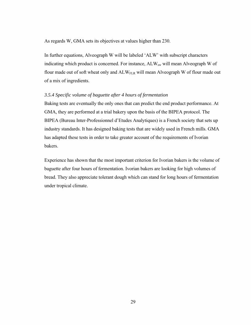
29

As regards W, GMA sets its objectives at values higher than 230.

In further equations, Alveograph W will be labeled ‘ALW’ with subscript characters

indicating which product is concerned. For instance, ALWsw will mean Alveograph W of

flour made out of soft wheat only and ALWFLR will mean Alveograph W of flour made out


3.5.4 Specific volume of baguette after 4 hours of fermentation

Baking tests are eventually the only ones that can predict the end product performance. At

GMA, they are performed at a trial bakery upon the basis of the BIPEA protocol. The

BIPEA (Bureau Inter-Professionnel d’Etudes Analytiques) is a French society that sets up

industry standards. It has designed baking tests that are widely used in French mills. GMA

has adapted these tests in order to take greater account of the requirements of Ivorian

bakers.

Experience has shown that the most important criterion for Ivorian bakers is the volume of

baguette after four hours of fermentation. Ivorian bakers are looking for high volumes of

bread. They also appreciate tolerant dough which can stand for long hours of fermentation

under tropical climate.

30

Figure 3.6: Volumeter test

Because the weights of baguettes are not always the same, this quality characteristic is

measured by a specific volume: the volume, in cubic centimeters, of one gram of baguette.

Volumes of baguettes are measured in a device called a “Volumeter” and their weights are

read on a laboratory balance.

According to GMA standards, the specific volume of a baguette after 4 hours of

fermentations should be higher than 11.5 cubic centimeters per gram.

31

Figure 3.7: Weighing baguettes

In further equations, the specific volume of a baguette after 4 hours of fermentation will be

labeled ‘BVL’ with subscript characters indicating which product is concerned. For

instance, BVLsw will mean specific volume of bread made out of soft wheat only and

BVLFLR will mean specific volume of bread made out of a mix of ingredients.

The following table summarizes GMA objectives as regards quality constraints.

Table 3.7: GMA quality specifications Quality Parameter Minimum Maximum

Flour Protein Content 11% 13%

Flour Falling Number 350 s. 500 s.

Flour Alveograph W 230

Specific volume of baguette after 4 hours of fermentation 11.5 cm3/gram

These specifications reflect the requirements of the Ivorian market in 2011/2012. They may

evolve in the future.

32

3.6 Quality constraints: equations (LHS)

The current section deals with the Left Hand Side (LHS) of the constraint equations: the

relationships between ingredients and quality parameters.

Grains science is the major source of information for defining these quality constraint

equations. Actually, most relationships between wheat, additives and flour characteristics

have already been studied and documented by grain scientists.

However, some specific relationships in the optimization model remain unknown. This is

the case when it comes to the specific volume of baguette. This is also the case when it

comes to enzymes mixes, because GMA has no precise information on their contents. In

such cases, regression analysis will be used in order to determine the relationships between

ingredients and flour quality parameters.

According to Ragsdale (2008, p. 409), “the goal in regression analysis is to identify a

function that describes, as closely as possible, the relationship between these (independent

and dependent) variables so that we can predict what value the dependent variable will

assume given specific values for the independent variables”. In other words, regression

analysis helps determine what the technical coefficients, βis, are in the constraints.

Table 3.8: Regression Analyses β coefficients

β0 + β1X1 +β2X2 + … + βnXn ≤ α, or

β0 + β1X1 +β2X2 + … + βnXn ≥ α, or

β0 + β1X1 +β2X2 + … + βnXn = α

where:

Xi are the independent variables ;

α is the dependent variable.

In the optimization model, Xi will represent some characteristics of soft wheat, hard wheat,

gluten, ascorbic acid or enzyme mixes and the different αs will stand for GMA

specifications as regards protein content, falling number, Alveograph W and baguette

specific volume.

33

Regression analyses will be performed on data collected by GMA in the past. GMA has

achieved tests of flour quality that were specially designed at gaining a better

understanding of the impacts of different inputs on the final product. Altogether 73 tests

were conducted in 2010 and 2011 with varying incorporation rates of soft wheat, hard

wheat, gluten, different enzyme mixes and/or ascorbic acid. Values of independent

variables and of corresponding dependent variables from all these tests are displayed in

Appendix B.

In the present thesis, regression analysis equations are determined using the Ordinary Least

Squares method, with the help of Microsoft Excel functions.

3.6.1 Flour protein content

Flour milling theory teaches that the flour protein content of a mix of wheat is the weighted

average of the flour protein contents of the different types of wheat that have been blended.

Flour millers also know that, in the range of protein contents used by GMA, the addition of

x% of gluten in flour will result in an increase of 0.8x% of protein content in the mix.

Accordingly, with an extraction rate of 80%, the addition of y% of gluten over wheat, will

result in an increase of (80% x 0.8y%) = 0.64y% of protein content in the mix.

Consequently, the protein content of a flour made out of soft wheat, hard wheat and gluten

is mathematically determined by the following equation.

Table 3.9: Equation FPC1 – Flour Protein Content

(Wsw/1000) FPCsw + (Whw/1000) FPChw + 0.64 (WGLT/1000) = FPCFLR

where:

Wsw, Whw and WGLT represent the weights in metric tons of respectively soft wheat, hard wheat

and gluten used in a mix, the total of which amounts to one thousand metric tons ;

FPCsw and FPChw and FPCFLR represent the protein contents of flours produced out of

respectively soft wheat and hard wheat and the final mix.

34

This equation has been tested against 10 analyses achieved by GMA of protein contents of

flours made exclusively out of wheat and gluten. The comparison of predicted flour protein

contents with actual ones is displayed in Appendix C.

The coefficient of correlation R between the two sets of data is equal to 0.87. Their

coefficient of determination R² is equal to 0.75, meaning that 75% of actual flour protein

content is explained by Equation FPC1. And the adjusted R² is equal to 0.72. All these

figures are high, confirming close correlation between flour protein contents predicted by

equation FPC1 and actual figures. In addition, a Student’s t test has been performed on the

two sets of data and concludes that the means of the two sets of data are the same (see

Appendix C).

This confirms that, when there are no other inputs than wheat and gluten, equation FPC1

above is valid.

Equation FPC1 has also been tested against other data, when other inputs, acid ascorbic and

different enzyme mixes, had been incorporated in the mix in addition to wheat and gluten.

Protein contents of 55 different flours made out of various ingredients were compared to

the results of equation FPC1. This test is displayed in Appendix D.

The coefficient of correlation R, the coefficient of determination R² and the adjusted R² of

the two new sets of data drop down to, respectively 0.80, 0.65 and 0.64. Such coefficients

are still high. However, the hypothesis stating that the means of the two sets of data are the

same, is not confirmed by a Student’s t test.

The drop in coefficients may be explained by the presence of ascorbic acid or enzyme

mixes. However, incorporation of ascorbic acid should have no effect on flour protein

content. Ascorbic acid does not contain proteins. As regards enzyme mixes, they may

contain protein but their rate of incorporation to the blend is so low that they should not

have a significant impact.

Consequently and because it is theoretically sound, FPC1 will be used as the flour protein

content constraint equation of the optimization model.

35

3.6.2 Flour falling number

Grains science has shown that the falling number of flour made out of a mix of wheat is not

the weighted average of the falling numbers of flours made out of its wheat components.

However, milling scientists have identified a proxy, the liquefaction number, which has this

desired characteristic. If FLN is the falling number, then the corresponding liquefaction

number LNR is equal to (6,000 / (FLN+50)).

The relationship between the liquefaction number of flour made from a mix of wheat and

the liquefaction numbers of flours made out of its wheat components can be written as

follows.

Table 3.10: Equation LNR1 – Liquefaction Number

(nw1LNRw1 + nw2LNRw2 + ….+ nwnLNRwn) = LNRFLR

where:

nw1, nw2 and nwn represent the relative proportion of n lots of wheat in the mix, the sum of nwi

being equal to 100% ;

LNRw1, LNRw2 … LNRwn represent the liquefaction numbers of flours produced out of the

respective lots of wheat 1,2 or n ;

LNRFLR represents the liquefaction number of flour made out of the mix of wheat.

Because it is much easier to use linear equations, liquefaction number will be used instead

of falling number in the equation of the optimization model. In Section 3.4, GMA falling

number specifications were fixed at 350 and 500 seconds. These standards now become

respectively 15.000 and 10.909 in terms of liquefaction numbers.

In further equations, liquefaction number will be labeled ‘LNR’ with subscript characters

indicating which product is concerned. For instance, LNRsw will mean liquefaction number

of flour made out of soft wheat only and LNRFLR will mean liquefaction number of flour

made out of a mix of ingredients.

For a blend weighing 1,000 metric tons that is made exclusively out of one lot of soft wheat

and one lot of hard wheat, equation LNR1 becomes:

36

Table 3.11: Equation LNR1 – Liquefaction Number – Soft wheat and hard wheat only

(Wsw/1000) LNRsw + (Whw/1000) LNRhw = LNRFLR

where:

Wsw and Whw represent the weights in metric tons of respectively soft wheat and hard wheat used

in a mix, the total of which amounts to one thousand metric tons ;

LNRsw and LNRhw represent the liquefaction numbers of flours produced out of respectively soft

wheat and hard wheat ;

LNRFLR represents the liquefaction number of flour made out of the mix of wheat.

This equation has been tested against 9 series of data GMA has recorded on falling

numbers or liquefaction numbers of flours made exclusively out of soft wheat and hard

wheat. The comparison between predicted liquefaction numbers and actual ones is

displayed in Appendix E.


coefficient of determination R² is equal to 0.28, meaning that 28% of actual liquefaction

number is explained by the theoretical equation. And the adjusted R² is equal to 0.17. A

Student’s t test, performed on the two sets of data, concludes that the means of the two sets

of data are the same. All these figures seem to confirm that there is a correlation between

liquefaction numbers predicted by equation LNR1 and actual figures. However, this

correlation is not very strong.

Differences between predictions from equation LNR1 and actual liquefaction numbers may

arise from many different sources. If wheat lots are not homogeneous enough, liquefaction

numbers from one sample may not represent the value of the whole lot. Because the test of

enzymatic activity is relatively sophisticated, the person who performs the test may also

influence the results. The devices with which tests are performed may also cause errors:

manufacturers of such devices acknowledge that tests performed on similar samples do not

always give the same results and the margin of error may be as high as five percent.

37

Although R² is smaller than expected, it can reasonably be assumed that, when there are no

other inputs than soft wheat and hard wheat, equation LNR1 above is confirmed by tests.

Equation LNR1 has also been tested against other data, when other ingredients such as

gluten, ascorbic acid or enzyme mixes have been incorporated in the mix in addition to

wheat. The comparison of the liquefaction numbers of 49 flours made out of different

ingredients and the results of equation LNR1 is displayed in Appendix F.

Surprisingly, coefficients R, R² and adjusted R² increase to 0.64, 0.41 and 0.39,

respectively. And a Student’s t test confirms that the means of the two sets of data are the

same. The fact that this second correlation is stronger than the previous one without

additives may come from the fact that it is tested against a larger dataset. However, other

ingredients should have no impact on falling number and, consequently, on liquefaction

number.

Gluten is composed of proteins and does not contain alpha-amylases. Ascorbic acid is not

an enzyme. The presence of these ingredients does not affect flour liquefaction number.

Enzyme mixes should increase the alpha-amylase activity of dough, as long as they contain

alpha-amylases. In their presence, falling number should decrease and liquefaction number

should increase. GMA has no information about the presence of alpha-amylases in its

enzyme mixes.

Regression analysis has been used in order to assess the relationship between enzyme

mixes and the proportion of flour liquefaction number which is not explained by wheat in

equation LNR1 above. The details of the regression analysis are shown in Appendix G. The

following table summarizes the Ordinary Least Squares estimates.

38

Table 3.12: Equation LNR2 – Liquefaction Number

LNRres = 1.7711 – 27.3652 WEN1 – 153.5047 WEN2

Standard deviation 21.0408 104.8242

t-statistic - 1.3006 - 1.4644

Adjusted R² = 0.0153 n = 39

where:

LNRres is the amount of liquefaction number that is not explained by the liquefaction numbers of

the mix of wheat ;

WEN1 and WEN2 are the weights, in metric tons, of respectively enzyme mix 1 and enzyme mix 2,

used in the mix, the total of which amounts to one thousand metric tons.

The adjusted R² is very low in the regression equation. Given their t-statistics, the

coefficients of WEN1 and WEN2 are not statistically significant at a level of 10%. In addition,

they are surprisingly negative. This poor regression equation may mean that there are no

alpha-amylases in the enzyme mixes used by GMA.

Consequently, equation LNR1 will be retained as the constraint equation of the

optimization model as regards flour liquefaction number.

3.6.3 Alveograph W

According to Chopin Technologies, the company that manufactures the Alveograph, W of

flour made out of a mix of wheat is equal to the weighted average of Ws of flours made out

of these different types of wheat. This can be mathematically translated as follows.

39

Table 3.13: Equation ALW1 – Alveograph W

(nw1ALWw1 + nw2ALWw2 + ….+ nwnALWwn) = ALWFLR

where:

nw1, nw2 and nwn represent respectively the relative proportion of n types of wheat in the mix, the

sum of nwi being equal to 100% ;

ALWw1, ALWw2 … ALWwn represent Alveograph Ws of flours produced out of the respective

types of wheat 1, 2 or n ;

ALWFLR represents the Alveograph W of flour made out of the mix of wheat.

When flour is made exclusively out of a blend of soft wheat and hard wheat and when the

total mix weighs 1,000 metric tons, equation ALW1 becomes.

Table 3.14: Equation ALW1 – Alveograph W – Soft wheat and hard wheat only

(Wsw/1000) ALWsw + (Whw/1000) ALWhw = ALWFLR

where:

Wsw and Whw represent the weights in metric tons of respectively soft wheat and hard wheat used

in a mix, the total of which amounts to one thousand metric tons ;

ALWsw and ALWhw represent Alveograph Ws of flours produced out of, respectively soft wheat

and hard wheat ;

ALWFLR represents the Alveograph W of flour made out of the mix of wheat.

This equation has been tested against 9 series of data GMA has recorded on flours made

exclusively out of soft wheat and hard wheat. The comparison between predicted Ws and

actual ones is displayed in Appendix H.


coefficient of determination R² is equal to 0.93, meaning that 93% of actual Alveograph W

is explained by the equation ALW1. And the adjusted R² is equal to 0.93. All these figures

confirm that there is a strong correlation between Alveograph W numbers predicted by

equation ALW1 and actual figures. A Student’s t test has been performed on the two sets of

data and it concludes that the means of the two sets of data are the same.

40

Equation ALW1 has also been tested against other data, when additives, gluten, acid

ascorbic or enzyme mixes had been incorporated into flour in addition to wheat. The

comparison of 55 Alveograph Ws from flours made out of different inputs and the results

of equation ALW1 is displayed in Appendix I.

The coefficient of correlation R, the coefficient of determination R² and the adjusted R²

between the two new sets of data drop down to, respectively 0.93, 0.87 and 0.87. These

coefficients nevertheless remain high. A Student’s t test confirms that the means of the two

sets of data are the same.

Theory supporting equation ALW1 is strong and is reinforced by tests on actual data.

Some additives may nevertheless have a further impact on Alveograph W. Gluten

reinforces pressure and extensibility of dough although this is generally considered as not

significant. Experience teaches that enzyme mixes may influence the strength of dough and

consequently Alveograph W. However, their impact is nevertheless difficult to forecast.

Regression analysis has been used in order to assess the relationship between gluten,

enzyme mixes and residual W, the amount of Alveograph W which is not explained by

wheat mixes. The details of the regression analysis are shown in Appendix J. The following

table summarizes the Ordinary Least Squares estimates.


ALWres = -0.6236 + 0.4938 WGLT + 110.3011 WEN1 + 272.3460 WEN2

St. deviation 0.4324 77.7021 398.1873

t-statistic 1.1421 1.4195 0.6840

Adjusted R² = 0.0868 n = 46

where:

ALWres is the amount of W that is not explained by the Ws of the mix of wheat ;

WGLT, WEN1 and WEN2 represent the weights, in metric tons, of respectively gluten, enzyme mix 1

and enzyme mix 2 used in a mix, the total of which amounts to one thousand metric tons ;

41

Adjusted R² is low at 0.0868. Signs of β coefficients are as expected. Only the β coefficient

of WEN1 is statistically significant at a level of 10%, according to the Student’s t-test.

Altogether this regression equation is not very satisfactory. But it is theoretically sound.

Consequently, ALW3, a mix of equations ALW1 and ALW2, will be used as the constraint

equation for Alveograph Ws in the optimization model.


(Wsw/1000) ALWsw + (Whw/1000) ALWhw – 0.6236 + 0.4938 WGLT + 110.3011 WEN1 + 272.3460 WEN2 = ALWFLR

3.6.4 Specific volume of baguette after 4 hours of fermentation

Unlike the other quality parameters, there is no readily available theoretical model that

links ingredients and flour as regards the specific volume of baguette after 4 hours of

fermentation. Only experience gives some hints.

Soft wheat, as the most important component of GMA mix is obviously a major influence

on the volume of baguettes. This influence is expressed in the specific volume of baguettes

made exclusively out of the soft wheat lot under review.

Incorporation of hard wheat at a relatively small percentage increases the volume of baguettes.

However, when this percentage is too high, it has an adverse effect. Stronger networks of

protein hinder the growth of dough. As already mentioned earlier, GMA does not make

baguettes out of its cargoes of hard wheat. In order to represent hard wheat influence in the

baguette specific volume constraints equation, a proxy, Alveograph W, ALWhw, the baking

strength of flour made exclusively out of hard wheat will be used.

Gluten has a similar effect as hard wheat on baguette volume. It brings higher gas retaining

power in dough. At relatively low incorporation rates, it favors high volume of bread. At

higher incorporation rates, it has an adverse effect.

The major reason for incorporating ascorbic acid into the mix is to increase bread volume.

Ascorbic acid brings oxygen in dough and helps breaking the protein network. It enhances

extensibility of dough, i.e. the ability of dough to expand while retaining gas.

42

Different enzymes may have different effects on the volume of bread. For instance,

glucose-oxidases favor bread volume while some proteases don’t. However, GMA requests

its supplier to elaborate enzyme mixes that increases bread volumes. One should therefore

expect that the effect of at least one of its enzyme mixes is positive when it comes to the

volume of baguettes.

In absence of a theoretical model, regression analysis is used in order to determine a

mathematical relationship between all these inputs and flour as regards the specific volume

of baguette after 4 hours of fermentation. Details of this analysis are displayed in Appendix

K. The following table summarizes the Ordinary Least Estimates.

Table 3.17: Equation BVL1 – Specific Volume of Baguette

BVLFLR = -1.0237 + 1.0482 (Wsw/1000) BVLsw + 0.0295 (Whw/1000) ALWhw

St. deviation 0.1523 0.0053

t-statistic 6.8839 5.5289

+ 0.00159 WGLT + 6.9306 WAAC + 23.0209 WEN1

St. deviation 0.0654 5.5136 5.9985

t-statistic 0.2437 1.2570 3.8378

+ 15.0943 WEN2

St. deviation 31.3419

t-statistic 0.4816

Adjusted R² = 0.6198 n = 66

where:

BVLFLR is the specific volume (volume divided by weight) expressed in cubic centimeters divided

by grams, of baguettes after 4 hours of fermentation ;

BVLsw is the specific volume (volume divided by weight) expressed in cubic centimeters divided

by grams, of baguettes, after 4 hours of fermentation, made from soft wheat only ;

ALWhw represents the Alveograph W of flour produced out of hard wheat only ;

43

Wsw, Whw, WGLT, WAAC, WEN1 and WEN2 represent the weights in metric tons of respectively soft

wheat, hard wheat, gluten, ascorbic acid, enzyme mix 1 and enzyme mix 2 used in a mix, the total

of which amounts to one thousand metric tons.

Adjusted R² is quite high at 0.62. Signs of β coefficients are positive as expected, except for

gluten. β coefficients are also statistically significant, according to Student’s t tests, except

for gluten, ascorbic acid and enzyme mix 2. Altogether this regression equation is relatively

satisfactory.

In between the limits of the technical constraints identified in Section 3.3 above, the

adverse effects of high incorporation rates of hard wheat and gluten should not be felt.

However, another way to take account of adverse effects is to use other functional forms in

the regression model. Equations with quadratic functions applied to hard wheat and gluten

have been tested. This regression analysis is documented in Appendix L and gives the

following results.

Table 3.18: Equation BVL2 – Specific Volume of Baguette

BVLFLR = -1.1560 + 1.0488 (Wsw/1000) BVLsw +

St. deviation 0.1543

t-statistic 6.7952

+ 0.0374 (Whw/1000) ALWhw + 0.0001 ((Whw/1000) ALWhw)2 +

St. deviation 0.0117 0.0001


- 0.0047 WGLT - 0.0050 (WGLT)2 + 6.9548 WAAC +

St. deviation 0.1427 0.0246 5.6151

t-statistic - 0.0331 - 0.2021 1.2386

+ 23.9619 WEN1 + 18.5955 WEN2

St. deviation 6.1970 32.1070


44

Adjusted R² = 0.6105 n = 66

where:

BVLFLR is the specific volume (volume divided by weight) expressed in cubic centimeters divided

by grams, of baguettes after 4 hours of fermentation ;

BVLsw is the specific volume (volume divided by weight) expressed in cubic centimeters divided

by grams, of baguettes, after 4 hours of fermentation, made from soft wheat only ;

ALWhw represents the Alveograph W of flour produced out of hard wheat only ;

Wsw, Whw, WGLT, WAAC, WEN1 and WEN2 represent the weights in metric tons of respectively soft

wheat, hard wheat, gluten, ascorbic acid, enzyme mix 1 and enzyme mix 2 used in a mix, the total

of which amounts to one thousand metric tons.

Adjusted R² in equation BVL2 is slightly lower than in equation BVL1. Signs of

coefficients of gluten are unexpectedly negative. According to Student’s t tests, the

coefficients of gluten, ascorbic acid and enzyme mix 2 are not statistically significant

Coefficients of negative squared weight of hard wheat W as well as negative squared

weight of gluten are also not statistically significant.

Because of the insignificance of the non-linear terms in equation BVL2, equation BVL1

has been preferred as the specific baguette volume constraint in the optimization model.

3.7 The optimization model

After identifying the objective function, the constraints, their limits and their equations, the

blending problem of GMA can be expressed in mathematical terms. The optimization

model includes an objective function and three types of constraints: self-binding

constraints, technical constraints and quality constraints.

3.7.1 The Objective Function

Table 3.19: Optimization Model – Objective Function MIN: (Wsw Psw) + (Whw Phw) + (WGLT PGLT) + (WAAC PAAC) + (WEN1 PEN1) + (WEN2 PEN2)

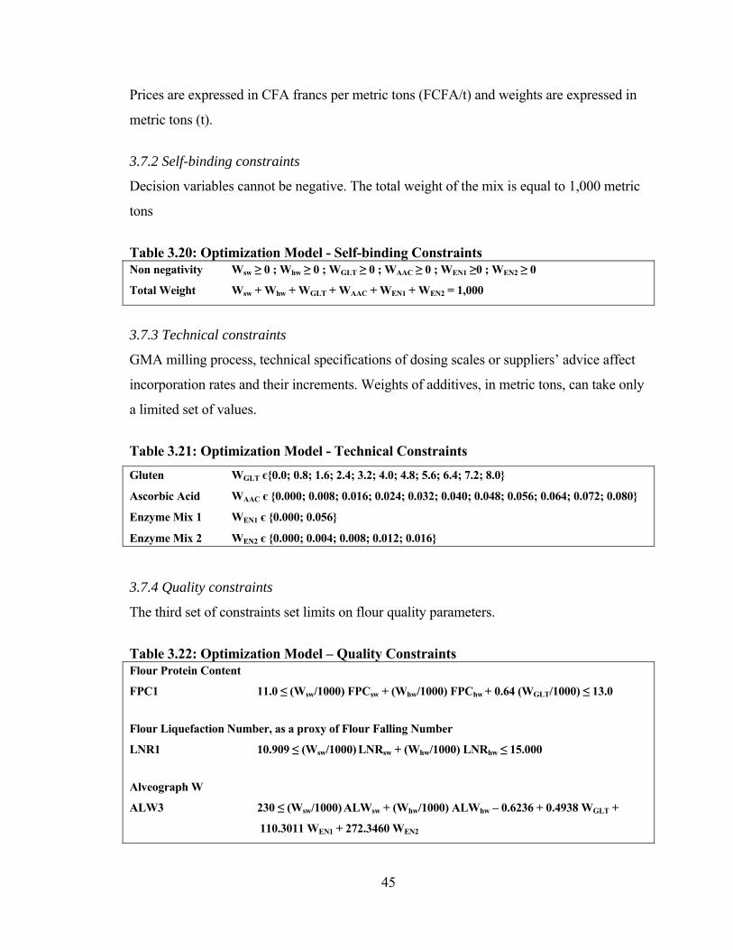
45

Prices are expressed in CFA francs per metric tons (FCFA/t) and weights are expressed in

metric tons (t).

3.7.2 Self-binding constraints

Decision variables cannot be negative. The total weight of the mix is equal to 1,000 metric

tons

Table 3.20: Optimization Model - Self-binding Constraints Non negativity Wsw ≥ 0 ; Whw ≥ 0 ; WGLT ≥ 0 ; WAAC ≥ 0 ; WEN1 ≥0 ; WEN2 ≥ 0

Total Weight Wsw + Whw + WGLT + WAAC + WEN1 + WEN2 = 1,000

3.7.3 Technical constraints

GMA milling process, technical specifications of dosing scales or suppliers’ advice affect

incorporation rates and their increments. Weights of additives, in metric tons, can take only

a limited set of values.

Table 3.21: Optimization Model - Technical Constraints

Gluten WGLT є{0.0; 0.8; 1.6; 2.4; 3.2; 4.0; 4.8; 5.6; 6.4; 7.2; 8.0}

Ascorbic Acid WAAC є {0.000; 0.008; 0.016; 0.024; 0.032; 0.040; 0.048; 0.056; 0.064; 0.072; 0.080}

Enzyme Mix 1 WEN1 є {0.000; 0.056}

Enzyme Mix 2 WEN2 є {0.000; 0.004; 0.008; 0.012; 0.016}

3.7.4 Quality constraints

The third set of constraints set limits on flour quality parameters.

Table 3.22: Optimization Model – Quality Constraints Flour Protein Content

FPC1 11.0 ≤ (Wsw/1000) FPCsw + (Whw/1000) FPChw + 0.64 (WGLT/1000) ≤ 13.0

Flour Liquefaction Number, as a proxy of Flour Falling Number

LNR1 10.909 ≤ (Wsw/1000) LNRsw + (Whw/1000) LNRhw ≤ 15.000

Alveograph W

ALW3 230 ≤ (Wsw/1000) ALWsw + (Whw/1000) ALWhw – 0.6236 + 0.4938 WGLT +

110.3011 WEN1 + 272.3460 WEN2

46

Specific volume of baguette after 4 hours of fermentation

BVL1 11.5 ≤ -1.0237 + 1.0482 (Wsw/1000) BVLsw + 0.0295 (Whw/1000) ALWhw +

0.0159 WGLT + 6.9306 WAAC + 23.0209 WEN1 + 15.0943 WEN2

The object of Chapter 3 was to transform GMA blending problem into a set of equations.

The real difficulty that appeared in this process was to make choices. The selection of

quality parameters, of their specifications (RHS), of the form of their equations (LHS) is at

least partly subjective and questionable. These choices do impact the results of the

optimization model.

47

CHAPTER IV: DATA AND METHODS COMPUTER IMPLEMENTATION

Nowadays, many spreadsheets provide tools, called solvers that easily solve optimization

model such as the one that has been identified in the previous Chapter.

In the first section of the present Chapter, one of these solvers will be considered. Then the

optimization model data will be entered on templates designed in Microsoft Excel.

4.1 Solver

Operational research and optimization techniques were first developed for military

purposes during World War II. Since then, these techniques have met an increasing

success. The different methods developed in order to solve an optimization model come

down to testing different solutions and selecting the optimal one. Efficient techniques like

the Simplex method allow for a low the number of iterations before finding the optimum

solution. However, solving a complex optimization problem nevertheless requires a

significant computing power. As a consequence, what really generalized the use of

operational research was the development of information systems and particularly personal

computers in the last decades of the 20th century. Spreadsheets and their solvers have made

it easy and simple to solve optimization problems.

Eventually, the implementation of the problem on computer has become a necessary and

ordinary step of the optimization modeling process. It is the third step of the five identified

by Ragsdale (2008) and it constitutes the fourth chapter of the present thesis.

Solvers are computer programs that are designed to find the values of certain cells, called

variable cells, which maximize or minimize the value of another cell, called a target cell,

while meeting problem constraints listed in other cells of the spreadsheet. In other terms,

solvers provide solutions to optimization problems.

There is a wide range of solver software available on the market nowadays. Some of them

are supplied on their own. Most often, they are included in spreadsheet packages. And

48

nowadays, any spreadsheet commonly integrates more or less sophisticated solver

functions.

For the purpose of the present thesis, the optimization model will be implemented on

Microsoft Office Excel 2010. Excel includes a solver function which was developed by a

company named Frontline Systems Inc. (www.solver.com).

However another solver, also developed by Frontline Systems Inc., and that work as an

Excel add-in will be preferred. Premium Solver V11.5 is more powerful then Excel Solver.

It includes a guided mode and it can handle larger and more complex models. It can be

purchased at a price of USD 4,000 which is worth about 2 million FCFA. This is cheap in

comparison of the price of one thousand tons of wheat. The cost of acquiring Premium

Solver V11.5 will therefore be neglected in the optimization model.

A drawback of Premium Solver V11.5 in a French-speaking country like Côte d’Ivoire is

that it is only available in English and it they must be added to the English version of

Microsoft Excel. The Excel Solver, on the other hand, is available on the French version of

Microsoft Excel.

Premium Solver V11.5 will be used and tested on two different models.

4.2 Models

In the previous Chapter, three types of constraints were identified: self-binding, quality and

technical constraints. The technical constraints limit the values that the weights of additives

can take. They drastically restrict the set of possible solutions to the optimization model.

Such constraints are equivalent to integrality conditions: decision variables can assume

only integer values.

A standard linear programming (LP) problem, where all variables are assumed to be

continuous has an infinite number of feasible solutions. An integer linear programming

(ILP) problem has only a finite set of feasible solutions. Integrality conditions may even

lead to infeasability.

49

In order to deal with this issue, two models will be built: an ILP model where all integrality

conditions are met, but also a LP model where the technical constraints are not considered.

If the ILP model does not find any solution, it can be relaxed. LP model solutions will then

be considered and may serve as substitutes.

Because it is easier to design and to implement, the LP model will be designed first.

Integrality conditions on additives will then be introduced in the ILP model

4.2.1 The LP Model

Microsoft Excel offers many ways to implement a LP model. Figure 4.1 shows one of

them.

Figure 4.1: LP optimization model on Excel

Quality parameters and prices of the different ingredients of the flour mix are inputs of the

model. They are highlighted in yellow. Variable cells, i.e. the weights of the different

ingredients in a mix of 1,000 metric tons, are highlighted are green. The target cell, the

50

price of the mix of 1,000 metric tons, is highlighted in blue. And finally, constraints are

highlighted in red.

Formula for cell J14, the target cell, is the sum of the prices of the different components of

the mix. Such prices are the products of unit prices (in row 12) by weights (in row 13). In

order to limit scaling problems, all prices are expressed in millions of CFA francs

(MFCFA).

The total weight of the mix is assumed to be equal to 1,000 metric tons, which is the first

constraint shown in cell K13. Data in cells C16:I19 record the different components (LHS)

of the quality constraints equations. The results of these equations are displayed in cells

J16:J19. These figures should be higher than constraints limits shown in cells K16:K19 and

lower than constraints limits shown in cells L16:L17 (RHS). Finally, cells E21:H21 show

the upper limits of the weights of additives in the mix.

In Excel, Premium Solver V11.5 is available in the Add-Ins menu. Target cell, variable

cells and constraints are entered into the Solver Parameters box, as displayed in Figure 4.2.

51

Figure 4.2: LP Premium Solver V11.5 Parameters box

Premium Solver V11.5 guided mode confirms that the model is LP convex.

52

Figure 4.3: LP Premium Solver V11.5 Guided mode

Several options can be defined in the Options box of Premium Solver V11.5.

Figure 4.4: LP Premium Solver V11.5 Options Box

53

Automatic Scaling is always useful although some of the scaling issues have already been

dealt with by using millions of CFA francs for prices.

Until now, technical constraints described in Section 3.3 have not been implemented in the

model.

4.2.3 The ILP model

The ILP model template is built on the basis of the LP model template. However, in order

to deal with the technical constraints, variables representing additives weights have been

redefined so that their respective increments correspond to one unit. With this conversion,

the model becomes an integer one: variable cells can assume only integer values. To do so,

variables Wi are replaced by their proxies Wi’.

Table 4.1: LP/ILP model - Units Correspondence Table Ingredients Formulas Wi units Wi’ units

Gluten WGLT’ = WGLT x1.25 1 metric ton 800 kg

Ascorbic acid WAAC’ = WAAC x 125 1 metric ton 8 kg

Enzyme Mix 1 WEN1’ = WEN1 x 1,000 / 56 1 metric ton 56 kg

Enzyme Mix 2 WEN2’ = WEN2 x 250 1 metric ton 4 kg

With such transformations, the technical constraints become:

Table 4.2: LP/ILP model - Technical Constraints Correspondence Table Ingredients Technical Constraints with Wi Technical Constraints with Wi’

Gluten WGLT є {0.0; 0.8; 1.6; 2.4; 3.2; 4.0; 4.8;

5.6; 6.4; 7.2; 8.0}

WGLT’ є {0; 1; 2; 3; 4; 5; 6; 7; 8; 9; 10}

Ascorbic acid WAAC є {0.000; 0.008; 0.016; 0.024; 0.032; 0.040; 0.048; 0.056; 0.064; 0.072; 0.080}

WAAC’ є {0; 1; 2; 3; 4; 5; 6; 7; 8; 9; 10}

Enzyme Mix 1 WEN1 є {0.000; 0.056}

WEN1’ є {0; 1}

Enzyme Mix 2 WEN2 є {0.000; 0.004; 0.008; 0.012; 0.016}

WEN2’ є {0; 1; 2; 3; 4}

Unit prices of ingredients are modified as well.

54

Table 4.3: LP/ILP model - Unit Prices Correspondence Table Ingredients Formulas Wi units Wi’ units

Gluten PGLT’ = PGLT / 1.25 1 metric ton 800 kg

Ascorbic acid PAAC’ = PAAC / 125 1 metric ton 8 kg

Enzyme Mix 1 PEN1’ = PEN1 / 1,000 x 56 1 metric ton 56 kg

Enzyme Mix 2 PEN2’ = PEN2 / 250 1 metric ton 4 kg

Coefficients of quality constraints also change, where weights of additives are concerned.

Table 4.4: LP/ILP model – Quality Constraints Correspondence Table Quality Constraint

Wi equations Wi’ equations

Flour protein Content 11.0 ≤ (Wsw/1000) FPCsw + (Whw/1000)

FPChw + 0.64 (WGLT/1000) ≤ 13.0

11.0 ≤ (Wsw/1000) FPCsw + (Whw/1000) FPChw + 0.512 (WGLT’ / 1000) ≤ 13.0

Flour Liquefaction Number

10,909 ≤ (Wsw/1000) LNRsw + (Whw/1000) LNRhw ≤ 15,000

10,909 ≤ (Wsw/1000) LNRsw + (Whw/1000) LNRhw ≤ 15,000

Alveograph W 230 ≤ (Wsw/1000) ALWsw + (Whw/1000)

ALWhw – 0.6236 + 0.4938 WGLT + 110.3011 WEN1 + 272.3460 WEN2

230 ≤ (Wsw/1000) ALWsw + (Whw/1000) ALWhw – 0.6236 + 0.3950 WGLT’ +

6.1769 WEN1’ + 1.0894 WEN2’

Specific Volume of Baguette 11.5 ≤ -1.0237 + 1.0482 (Wsw/1000)

BVLsw + 0.0295 (Whw/1000) ALWhw +

0.0159 WGLT + 6.9306 WAAC + 23.0209 WEN1 + 15.0943 WEN2

11.5 ≤ -1.0237 + 1.0482 (Wsw/1000) BVLsw + 0.0295 (Whw/1000) ALWhw +

0.0127 WGLT’ + 0.0554 WAAC’ + 1.2892 WEN1’ + 0.0604 WEN2’

Finally, the sum of the weights of ingredients, which is assumed to be equal to 1,000 metric

tons, was straightforward in the LP model. It now becomes.

Table 4.5: LP/ILP model – Sum of Weights Correspondence Table LP model / Wi equations ILP model / Wi’ equations

Wsw + Whw + WGLT + WAAC + WEN1

+ WEN2 = 1,000

Wsw + Whw + (WGLT' / 1.25) + (WAAC' /125) + (WEN1' x 56 /

1000) + (WEN2' / 250) = 1,000

This new ILP model can be implemented in Excel as seen in Figure 4.5.

55

Figure 4.5: ILP optimization model on Excel

Unit prices, total weight, constraints formulas and limits have been changed. And a new

constraint has been introduced: additives weights must be integer figures.

Figure 4.6: ILP Premium Solver V11.5 Parameters Box

56

The integer options box has also been fulfilled and integer optimality set to 0% as shown in

Figure 4.7. With this option, the model does not allow any tolerance on the constraints.

Figure 4.7: ILP Premium Solver V11.5 Options Box

Unlike the LP Model, the ILP model integrates all constraints.

The set of equations and inequalities of the optimization model has been translated into two

spreadsheet templates. Premium Solver V11.5 has been fed with the model parameters. The

optimization model, in its two versions, LP and ILP, is now ready to be tested with actual

data.

57

CHAPTER V: RESULTS

The GMA blending problem has been put into a mathematical programming model and

implemented on computer. The optimization model is ready to be solved and tested.

Four months when GMA has made blending decisions have been selected: February 2011,

May 2011, August 2011 and February 2012. Corresponding data have been entered in the

model templates.

In the first section, the optimization model solutions will be described. In the second

section, they will be discussed. Finally, in the third section, a special attention will be given

to the quality constraints equations that were identified in Chapter 3.

5.1 Results

In the months being considered, GMA processed soft wheat and hard wheat with the

following characteristics.

Table 5.1: Soft wheat quality parameters Period Feb. 2011 May 2011 Aug. 2011 Feb. 2012

Vessel African Orchyd

Silva- plana

Lavaux Monte Azul

Flour Protein Content (%) 10.7 10.8 10.8 11.1

Flour Falling Number (s.) 372 325 354 339

Alveograph W 225 207 235 250

Specific weight of baguette after 4 hours of fermentation (cm3/g)

11.88 11.40 10.52 12.55

Table 5.2: Hard wheat quality parameters Period Feb. 2011 May 2011 Aug. 2011 Feb. 2012

Vessel Amorita Greenwing Federal Leda

Neptune Pioneer

Flour Protein Content (%) 15.7 15.6 15.4 15.8

Flour Falling Number (s.) 468 424 598 430

Alveograph W 457 415 387 475

Prices of the different ingredients, in FCFA/t, as recorded in GMA books, were as follows.

58

Table 5.3: Unit prices of ingredients Prices (FCFA/t) Feb. 2011 May 2011 Aug. 2011 Feb. 2012

Soft Wheat 219,680 229,302 212,644 188,669

Hard Wheat 221,321 241,044 230,980 245,530

Gluten 1,286,000 1,238,000 1,579,000 1,204,900

Ascorbic acid 5,711,000 5,245,570 5,245,570 4,415,180

Enzyme mix 1 26,957,570 26,957,570 27,255,950 27,255,950

Enzyme mix 2 24,752,100 24,752,100 24,752,100 24,752,100

With these data as inputs, Premium Solver V11.5 gives the following LP optimal solution,

as regards February 2011.

Figure 5.1: Premium Solver V11.5 - LP optimization model – February 2011

59

Premium Solver V11.5 gives a different solution to the ILP model.

Figure 5.2: Premium Solver V11.5 - ILP optimization model – February 2011

Figures 5.1 and 5.2 are screen captures from Microsoft Excel. Premium Solver V11.5 can

also display optimal solutions as an Answer Report.

60

Figure 5.3: Premium Solver V11.5 - ILP Answer Report – February 2011

The following tables compare, for each month under review, the LP model solutions, the

ILP model solutions and the blend that was actually implemented by GMA.

Microsoft Excel 14.0 Answer Report

Worksheet: [Feb 11 ILP PSP.xlsx]Template ILP

Report Created: 9/8/2012 11:57:40 AM

Result: Solver found a solution. All constraints and optimality conditions are satisfied.

Engine: Standard LP/Quadratic

Solution Time: 01 Seconds

Iterations: 0

Subproblems: 0

Incumbent Solutions: 0

Objective Cell (Min)

Cell Name Original Value Final Value

$J$16 Target Cell Total 219,7930115 219,7930115

Decision Variable Cells

Cell Name Original Value Final Value Type

$C$15 Weights sw 930,9116 930,9116 Normal

$D$15 Weights hw 69,0884 69,0884 Normal

$E$15 Weights GLT 0,0000 0,0000 Normal

$F$15 Weights AAC 0,0000 0,0000 Normal

$G$15 Weights EN1 0,0000 0,0000 Normal

$H$15 Weights EN2 0,0000 0,0000 Normal

Constraints

Cell Name Cell Value Formula Status Slack

$J$15 Weights Total 1000,0000 $J$15=$K$15 Binding 0

$J$18 Flour Protein Content Total 11,0 $J$18<=$L$18 Not Binding 1,954557754

$J$19 Flour Liquefaction Number Total 14,036 $J$19<=$L$19 Not Binding 0,96403844

$J$18 Flour Protein Content Total 11,0 $J$18>=$K$18 Not Binding 0,045442246

$J$19 Flour Liquefaction Number Total 14,036 $J$19>=$K$19 Not Binding 3,126870651

$J$20 Alveograph W Total 240 $J$20>=$K$20 Not Binding 10,40492022

$J$21 Specific Volume of Bread Total 11,5 $J$21>=$K$21 Binding 0

$E$15 Weights GLT 0,0000 $E$15<=$E$23 Not Binding 10

$F$15 Weights AAC 0,0000 $F$15<=$F$23 Not Binding 10

$G$15 Weights EN1 0,0000 $G$15<=$G$23 Not Binding 1

$H$15 Weights EN2 0,0000 $H$15<=$H$23 Not Binding 4

61

Table 5.4: LP and ILP optimal solutions vs. actual ones February 2011 LP Model ILP model Actual Blend

(tons)

Soft Wheat 939.9958 930.9116 947.6668

Hard Wheat 60.0029 69.0884 49.8772

Gluten 2.4000

Ascorbic acid 0.0014

Enzyme Mix 1 0.0560

Enzyme Mix 2

Total Weight 1,000.0000 1,000.0000 1,000.0000

Price MFCFA 219.7855 219.7930 223.8180

May 2011 LP Model ILP model Actual Blend

(tons)

Soft Wheat 701.0240 701.0303 949.9886

Hard Wheat 298.9057 298.8977 49.9994

Gluten

Ascorbic acid 0.0703 0.0720

Enzyme Mix 1

Enzyme Mix 2 0.0120

Total Weight 1,000.0000 1,000.0000 1,000.0000

Price MFCFA 233.1643 233.1725 230.1830

August 2011 LP Model ILP model Actual Blend

(tons)

Soft Wheat 956.1192 956.2271 947.6668

Hard Wheat 43.7606 43.6849 49.8772

Gluten 2.4000


Enzyme Mix 1 0.0402 0.0560 0.0560

Enzyme Mix 2

Total Weight 1,000.0000 1,000.0000 1,000.0000

Price MFCFA 214.9376 215.1207 218.3525

62

February 2012 LP Model ILP model Actual Blend

(tons)

Soft Wheat 854.9451 854.9451 899.9496

Hard Wheat 145.0549 145.0549 99.9944

Gluten

Ascorbic acid

Enzyme Mix 1 0.0560

Enzyme Mix 2

Total Weight 1,000.0000 1,000.0000 1,000.0000

Price MFCFA 196.9173 196.9173 195.8709

The solutions provided by the optimization model are alternatives to the blends that were

actually implemented by GMA. They make sense and, in two cases out of four, are cheaper

than actual blends. However, they must be considered in more depth.

5.2 Discussion

The different solutions provided by the optimization models need to be assessed. In the

following paragraphs, the following points will be addressed:

Different LP model solutions and ILP model solutions;

Optimization model solutions and actual blends.

5.2.1 Different optimization model solutions: LP vs. ILP

In February 2012, solutions of the LP model and of the ILP model are the same. In the

other 3 months, solutions of the LP model are, logically, cheaper than solutions of the ILP

model since ILP models include more constraints (technical constraints) than the LP

models.

An alternative way to introduce the technical constraints into the optimization model would be

to round the decision variables of the LP model solutions to the next values that belong to the

set of admitted weights for additives.

63

Table 5.5: Rounded LP optimal solutions Weights in tons Feb. 2011 May 2011 Aug. 2011

Soft Wheat 940.000 701.0172 956.1040

Hard Wheat 60.000 298.9028 43.7600

Gluten


Enzyme Mix 1 0.0560

Enzyme Mix 2

Total Weight 1,000.0000 1,000.0000 1,000.0000

Total Price (MFCFA) 219.7781 233.2127 215.3637

The rounded LP optimal solution for February 2011 (219.7781 MFCFA) is cheaper than

both LP optimal solution (219.7855 MFCFA) and ILP optimal solution (219.7930

MFCFA). However, with this rounded LP optimal solution, the specific volume of baguette

after 4 hours of fermentation is predicted to go down to 11.49 cm3 against a minimum fixed

at 11.50 cm3.

Figure 5.4: Rounded LP optimization model – February 2011

64

When it comes to May 2011, all quality constraints are met by the rounded LP optimal

solution. However, its total price is more expensive (233.2127 MFCFA) than both the LP

optimal solution (233.1643 MFCFA) and ILP optimal solution (233.1725 MFCFA).

The same thing happens in August 2011. All quality constraints are met but the total price

of the rounded LP solution (215.3637 MFCFA) is more expensive than both the LP optimal

solution (214.9376 MFCFA) and ILP optimal solution (215.1207 MFCFA).

LP solutions and rounded LP solutions, although theoretically questionable, are

nevertheless interesting. They require less computing power from solvers than ILP: the

Excel Solver is powerful enough to provide the same solutions as Premium Solver V11.5.

However, rounding of LP solutions may end up with solutions that do not respect all

quality constraints or that are not optimal.

5.2.2 Optimization model solutions vs. actual blends

Blends that were actually implemented by GMA never correspond to optimal solutions of

the model, whether LP or ILP. Different reasons may explain this fact.

a) Routine thinking

One can note that the blend that has actually been implemented in August 2011 is the same

as the one that had already been implemented in February 2011. This may be the effect of

some routine thinking. The chief miller may use solutions that have worked previously

rather than take risks with a new blend. If this assumption is true, it reinforces the interest

of the optimization model for GMA management since the optimization model may be

more imaginative than the chief miller.

b) Hidden constraints

It is also remarkable that the weights of hard wheat that are suggested by the optimization

model for May 2011 and February 2012 are much larger than in actual blends. However, if

GMA had applied these solutions, it would have had to order a vessel of hard wheat four or

five times earlier than scheduled. One may assume that the chief miller does not want to be

short of hard wheat and that, when he makes a decision, he takes account of the inventory

of supplies.

65

Something similar happens with enzyme mixes. Their incorporation is suggested by the

optimization model in August 2011 only. On the other hand, the chief miller has actually

used such mixes in all four months. This may be because enzyme mixes have limited shelf

life. If GMA does not use these enzyme mixes, it will have to throw them away.

These two considerations show that there are some hidden constraints that are not taken

into account by the optimization model. One must not forget that modeling is a process that

simplifies reality and sometimes reality is more complex than expected.

c) Potential savings

The following tables compare the prices of the ILP optimal solutions and of the actual

blends.

Table 5.6: Price of optimal solutions vs. actual blends Price

(MFCFA/1,000 t.)

Feb. 2011 May 2011 Aug. 2011 Feb 2012 Total

ILP model 219.7930 233.1725 215.1207 196.9173 865.0035

Actual blend 223.8180 230.1830 218.3525 195.8709 868.2244

Difference (Actual – ILP)

4.0250 - 2.9895 3.2318 - 1.0464 3.2209

The purchase of 4,000 metric tons of ingredients, i.e. 1,000 metric tons in each month of

February 2011, May 2011, August 2011 and February 2012 according to the suggestions of

the ILP optimization model would have cost 865.0035 MFCFA against 868.2244 MFCFA

actually paid by GMA. The difference (868.2244 – 865.0035) = 3.2209 corresponds to

0.805 MFCFA per thousand tons. Since GMA processes some 250,000 tons of ingredients

per year, one can infer that the optimization model could enable GMA to save some

201.3 MFCFA per year. This sum is worth about 400,000 US dollars. The optimization

model may indeed help GMA reduce its costs of production.

d) Quality specifications, binding constraints and sensitivity analyses

Optimization model solutions are not always the cheapest ones. In May 2011 and February

2012, actual blends are cheaper than optimization model solutions. This happens because

66

all constraints are not met by actual blends. The following tables show the values of the

different quality parameters as computed by equations defined in Chapter 3 and applied to

the different mixes.

Table 5.7: Quality constraints of optimal vs. actual solutions February 2011 Limits LP model ILP model Actual

Flour Protein Content 11.0% ≤ x ≤ 13.0% 11.0% 11.0% 10.9%

Flour Falling Number 350s. ≤ x ≤ 500s. 377s. 377s. 377s.

Alveograph W 230 ≤ x 238 240 243

Specific volume of baguette 11.5 cm3 ≤ x 11.5 cm3 11.5 cm3 12.8 cm3

May 2011 Limits LP model ILP model Actual



Alveograph W 230 ≤ x 269 269 220


August 2011 Limits LP model ILP model Actual



Alveograph W 230 ≤ x 245 247 249

Specific volume of baguette 11.5 cm3 ≤ x 11.5 cm3 11.5 cm3 11.3cm3

February 2012 Limits LP model ILP model Actual



Alveograph W 230 ≤ x 282 282 278


When it comes to actual blends, parameters highlighted in yellow do not respect GMA

quality specifications.

67

In addition to optimal solutions, solvers provide information about binding constraints, i.e.

constraints which are strictly satisfied in the optimal solution, with no slack. The following

table displays, for instance, the Answer report for February 2011 ILP Model. This report

outlines the fact that the specific volume of baguette is a binding constraint.

Figure 5.5: ILP optimization model – February 2011 Answer Report

The following tables compare the binding quality constraints of the LP and the ILP models

and the constraints that were not met by actual blends.

Table 5.8: Optimal solutions binding constraints and quality parameters of actual blends February 2011 Constraints LP model ILP model Actual

Flour Protein Content 11.0% ≤ x X X

x ≤ 13.0%

Flour Falling Number 350s. ≤ x

x ≤ 500s.

Alveograph W 230 ≤ x

Specific volume of baguette 11.5 cm3 ≤ x X X

68

May 2011 Constraints LP model ILP model Actual

Flour Protein Content 11.0% ≤ x

x ≤ 13.0%

Flour Falling Number 350s. ≤ x X X X

x ≤ 500s.

Alveograph W 230 ≤ x X


August 2011 Constraints LP model ILP model Actual

Flour Protein Content 11.0% ≤ x X X

x ≤ 13.0%

Flour Falling Number 350s. ≤ x

x ≤ 500s.



February 2012 Constraints LP model ILP model Actual

Flour Protein Content 11.0% ≤ x

x ≤ 13.0%

Flour Falling Number 350s. ≤ x X X X

x ≤ 500s.


Specific volume of baguette 11.5 cm3 ≤ x

In all four months of the sample, constraints that were not met by actual blends correspond

to optimization models binding constraints. Optimization models can effectively identify

the most sensitive constraints.

But solvers can go further than that. They provide Sensitivity reports for LP models. These

reports give information about the consequences of relaxing binding constraints.

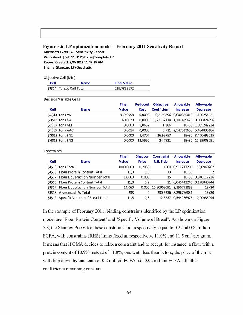
69

Figure 5.6: LP optimization model – February 2011 Sensitivity Report

In the example of February 2011, binding constraints identified by the LP optimization

model are "Flour Protein Content" and "Specific Volume of Bread". As shown on Figure

5.8, the Shadow Prices for these constraints are, respectively, equal to 0.2 and 0.8 million

FCFA, with constraints (RHS) limits fixed at, respectively, 11.0% and 11.5 cm3 per gram.

It means that if GMA decides to relax a constraint and to accept, for instance, a flour with a

protein content of 10.9% instead of 11.0%, one tenth less than before, the price of the mix

will drop down by one tenth of 0.2 million FCFA, i.e. 0.02 million FCFA, all other

coefficients remaining constant.

Microsoft Excel 14.0 Sensitivity Report

Worksheet: [Feb 11 LP PSP.xlsx]Template LP

Report Created: 9/8/2012 11:47:19 AM

Engine: Standard LP/Quadratic

Objective Cell (Min)

Cell Name Final Value

$J$14 Target Cell Total 219,7855172

Decision Variable Cells

Final Reduced Objective Allowable Allowable

Cell Name Value Cost Coefficient Increase Decrease

$C$13 tons sw 939,9958 0,0000 0,2196796 0,000825019 1,160254621

$D$13 tons hw 60,0029 0,0000 0,22132114 1,702429678 0,000824896

$E$13 tons GLT 0,0000 1,0652 1,286 1E+30 1,065242224

$F$13 tons AAC 0,0014 0,0000 5,711 2,547523653 5,494835186

$G$13 tons EN1 0,0000 8,4707 26,95757 1E+30 8,470695015

$H$13 tons EN2 0,0000 12,5590 24,7521 1E+30 12,55903251

Constraints

Final Shadow Constraint Allowable Allowable

Cell Name Value Price R.H. Side Increase Decrease

$J$13 tons Total 1000,0000 0,2080 1000 0,912217206 53,0960267

$J$16 Flour Protein Content Total 11,0 0,0 13 1E+30 2

$J$17 Flour Liquefaction Number Total 14,060 0,000 15 1E+30 0,940117226

$J$16 Flour Protein Content Total 11,0 0,2 11 0,045442246 0,178840744

$J$17 Flour Liquefaction Number Total 14,060 0,000 10,90909091 3,150791865 1E+30

$J$18 Alveograph W Total 238 0 230,6236 8,296766831 1E+30

$J$19 Specific Volume of Bread Total 11,5 0,8 12,5237 0,544276976 0,00935096

70

GMA may have to consider such constraints modifications. Premium Solver V11.5

provides all the relevant information that is necessary to make such a decision. The

optimization model enables GMA management to take such a decision with full knowledge

of its consequences, in terms of price as well as in terms of quality.

Up till now, the values of quality constraint parameters have been computed by the

equations of the optimization model as they were determined in Chapter 3. Obviously, such

values are true only if these quality constraint equations hold. It is therefore important to

test these quality constraint equations.

5.3 Optimization model quality constraints equations.

GMA laboratory performs flour tests on a daily basis. At least one sample of flour

produced per work shift is tested on its rheological and milling properties. At least one

sample of flour per working day is transformed into bread in the test bakery.

The results of these tests for February 2011, May 2011, August 2011 and February 2012

are displayed in Appendix M.

Results of laboratory tests have been compared with the results of the equations of the

optimization model. They have also been used to check whether actual blends respect

GMA quality specifications.

5.3.1 Test of quality constraint equations

Quality parameters of actual flour samples are analyzed by GMA laboratory and GMA test

bakery.

Table 5.9: Quality parameters of actual samples of flour February 2011 Average Standard

Deviation

Number of

tests

Flour Protein Content 10.9% 0.2 24

Flour Falling Number 368s. 12 24

Alveograph W 240 15 24

Specific volume of baguette 12.46 cm3/g 0.42 9

71

May 2011 Average Standard

Deviation

Number of

tests





August 2011 Average Standard

Deviation

Number of

tests





February 2012 Average Standard

Deviation

Number of

tests





These tests have been conducted on samples. If one assumes that the four quality

parameters are normally distributed, then the 99.74 percent confidence interval of the

population means is determined by the following formula.

Table 5.10: Normal Distribution Confidence Intervals [ m - 3σ/√n ; m + 3σ/√n ]

where:

m is the average of the sample ;

σ is the standard deviation of the sample ;

n is the size of the sample.

72

The following table compares, for each period and each quality parameter:

values computed by optimization model equations and

confidence intervals of the population means, determined upon the basis of sample tests.

Table 5.11: Quality parameters: computed figures vs. confidence intervals February 2011 Optimization

model

equations

Confidence

Interval

lower limit

Confidence

Interval

upper limit

Flour Protein Content 10.9% 10.8% 11.0%

Flour Falling Number 377s. 361s. 376s.


Specific volume of baguette 12.80 cm3/g 12.04 cm3/g 12.88 cm3/g

May 2011 Optimization

model

equations

Confidence

Interval

lower limit

Confidence

Interval

upper limit





August 2011 Optimization

model

equations

Confidence

Interval

lower limit

Confidence

Interval

upper limit





73

February 2012 Optimization

model

equations

Confidence

Interval

lower limit

Confidence

Interval

upper limit





Values highlighted in yellow are outside of the confidence intervals. The following table

summarizes the cases when values computed by optimization model equations fall into or

outside the limits of the confidence intervals.

Table 5.12: Quality parameters: computed figures vs. confidence intervals - Summary Feb. 2011 May 2011 Aug. 2011 Feb. 2012

Flour Protein Content IN IN IN OUT

Flour Falling Number OUT OUT IN IN

Alveograph W IN IN IN IN

Specific volume of baguette IN OUT OUT OUT

Altogether, computed figures are in between the limits of the confidence intervals in nine

cases out of sixteen.

Flour Protein Content equation FPC1 is exclusively based upon Grains Science knowledge.

This equation gives results that fall within confidence intervals limits, in three out of four

cases.

Flour Falling Numbers in the optimization model are computed with Flour Liquefaction

Numbers equation LNR1. This equation has been built upon theory because econometrics

did not bring significant results. However, the correlation between the equation results and

GMA data was not very strong. Only two out of four results are inside the confidence

intervals.

74

The Alveograph W equation ALW3 is designed out of both theory and econometrics. The

model equation gives four results that are inside confidence intervals.

The specific volume of baguette equation BVL1 is determined exclusively by

econometrics. The results of this equation lie outside the limits of the confidence intervals

three times out of four.

These results outline the need for GMA to improve the optimization model by enhancing

the validity and robustness of the quality constraints equations. This is particularly true

when regression analysis is involved. Further econometrics research should be made more

specifically on “Flour falling number” and on “Specific volume of baguette after 4 hours of

fermentation”.

5.3.2 Actual flour and quality specifications

Actual flour quality parameters, measured by confidence intervals, have also been tested

against GMA quality specifications.

Table 5.13: Flour quality standards vs. actual GMA

specifications

Feb. 2011 May 2011 Aug. 2011 Feb. 2012

Flour Protein Content

11.0% ≤ x ≤ 13.0%

[10.8% - 11.0%]

[10.9% - 11.0%]

[11.0%-11.1%]

[11.2%-11.3%]

Flour Falling Number

350s. ≤ x ≤ 500s. [361 – 376] [356-372] [356-365] [343-350]

Alveograph W 230 ≤ x [231 – 249] [217-234] [238-249] [264-282] Specific volume of baguette

11.5 cm3 ≤ x [12.04-12.88] [11.74–12.71] [12.19-12.54] [12.71-13.31]

At worst, confidence intervals of actual flour quality parameters have common limits with

GMA specifications. These worst cases are highlighted in yellow. Under such

circumstances, one cannot reject the claim that GMA flour respects its quality standards.

The chief miller’s experience may be a better predictor of flour quality than the

optimization model quality equations.

GMA managers must be aware that the optimization model is no more valid than its

assumptions. This observation leads to two remarks.

75

First, there is a need to improve quality constraints equations. Actual blends of May 2011

and February 2012 are cheaper than ILP optimization model solutions and, although quality

constraints equations tell another story, one cannot prove that this happens because quality

parameters are not respected.

Then, one must not forget that all the conclusions of this section are subject to the

assumption that the four quality parameters are normally distributed. This may be true but

laboratory tests are subject to biases.

76

CHAPTER VI :SUMMARY AND CONCLUSIONS

The objective of the present thesis, as it is defined in Chapter 1 is to determine the optimal

blend of wheat and additives that minimizes flour millers’ cost of production while meeting

quality requirements.

This objective has been achieved. The objective function and the constraints of GMA have

been translated into mathematical equations. The set of equations and inequalities has been

implemented in Microsoft Office Excel 2010. Premium Solver V11.5 has found optimal

solutions to several examples of actual business situations.

Figure 6.1: GMA flour mill staff

These optimization model solutions do question the habits of the chief miller, without any

prejudice. And it can be inferred from these examples that the implementation of these

optimal solutions would overall have saved money for GMA when compared with actual

blends. However, on a case by case basis, money saving is not always true.

Some observations need to be made and several limitations remain.

77

Choosing a solver: ILP vs. LP model

The optimization model takes account of technical constraints such as dosing scales

capacities or additives suppliers’ advice. They limit the set of values that additives

weights can take in the blend and transform the model into an Integer Linear

Programming (ILP) problem instead of a simpler Linear Programming (LP) one. ILP

models require powerful solvers. However, Premium Solver V11.5 is effective at solving

GMA ILP optimization model.

If technical constraints are neglected and only quality constraints are considered, Excel

Solver is sufficient to solve the LP optimization model. Excel Solver has several

advantages: it is easy to implement, it is free of additional charge and it is available in

French. On the other hand, solutions provided by the LP optimization model may be

irrelevant. Rounding of LP solutions may lead to solutions that do not respect quality

constraints.

Assessing the assumptions

In order to build quality constraints, several important assumptions were made. These

assumptions should not be taken for granted. They need to be questioned and periodically

revised. The following considerations must be taken account of:

1. Selecting quality parameters

Four quality parameters were selected to represent the expectations of GMA customers:

flour protein content, flour falling number, Alveograph W and the specific volume of

baguettes after 4 hours of fermentation. The choice of these parameters is supported by

previous literature, some econometrics and the experience of the Ivorian market. It is

nevertheless at least partly subjective and should be reassessed from time to time.

2. Setting limits (RHS) to quality parameters

The limits that are assigned to quality parameters are designed in order to fit with market

requirements. They should reflect the evolution of the market.

3. Determining quality (LHS) constraint equations

The LHS of the quality equations describe the way ingredients impact flour quality

parameters. Equations have been determined with reference to grains science theory and

78

with the help of econometrics. The comparison of the results of these equations and test

analyses of actual flour shows that quality constraint equations should be further

researched and improved.

Improved quality constraint equations are particularly important when GMA wants to

assess, with the help of sensitivity reports from solvers, the possibility of relaxing its

quality specifications.

Keeping hidden constraints in mind

The comparison between optimization model solutions and actual blends shows that the

model does not take account of some hidden constraints such as the delivery program of

hard wheat or expiration dates for consumption of ingredients. GMA management should

be cautious about the possible existence of such hidden constraints when considering the

solutions provided by the optimization model.

More generally, the main problems encountered during this thesis did not lie with

optimization techniques. The most important issues boil down to modeling the economic

reality. Reality is often too complex to be easily and fully grasped into an economic

model. However, although perfectible, the optimization model designed in the present

thesis has proven to be of interest for GMA in providing challenging ideas for

minimizing costs of production while still meeting quality requirements.

The next step will be to implement the model and to use it as frequently as possible when

blending decisions are to be made. This way, the advantages but also the limitations and

imperfections of the model will be revealed. Hopefully GMA will save money with the

help of this model and this will enhance the interest in correcting its imperfections.

79

WORKS CITED

Charnes, A., W.W. Cooper and A. Henderson. An Introduction to Linear Programming. Wiley, New York, 1953. Chopin Technologies http://www.chopin.fr (accessed September 8, 2012° Del Frate, Régis. “Mieux Connaître la Farine.” Les Nouvelles de la Boulangerie Pâtisserie 85 (January 2005): 2-15 Fowler, Mark. “Blending for Value.” World Grain, October 2009. Frontline Systems Inc. – Risk Solver Platform V11.5 2012 - http://www.solver.com (accessed September 1, 2012). Hayta, Mehmet and Cakmakli Ünsal. “Optimization of Wheat Blending to Produce Breadmaking Flour.” Journal of Food Process Engineering 24 (2001): 179-192 Lloyd, Peter. “Wheat Blend Calculator.” Spreadsheet model presented by US Wheat Associates, Casablanca, May 2005 Niernberger, Floyd F. “Blending Wheat to Meet Product Specifications.” Bulletin-Association of Operative Millers (September 1973): 3395-3400 Perten Instruments http://www.perten.com (accessed September 8, 2012) Ragsdale, Cliff T. Spreadsheet Modeling & Decision Analysis. Thomson-South Western, 2008 Schurle, Bryan and Mark Fowler. “Spreadsheet Solutions.” Lesson of the Flour Milling Short Course, International Grains Program, Kansas State University, June 5-16, 2006 Steuer, R.E. Multi-Criteria Optimization: Theory, Computation, and Application. John Wiley & Sons, New York, 1986 Studenmund, A.H. Using Econometrics. Pearson-Addison Wesley, 2006

80

APPENDIX A: ANALYSIS OF REDUNDANCY (CORRELATION) OF QUALITY

PARAMETERS

1. Analyses Data

ANAL

YSES

DATA

Refere

nce01/

2010

02/201

003/

2010

04/201

005/

2010

06/201

007/

2010

08/201

009/

2010

11/201

012/

2010

13/201

014/

2010

15/201

017/

2010

18/201

019/

2010

21/201

0Da

te20-

janv-10

02-févr

-1003-

mars-1

023-m

ars-10

08-avr

-1029-

avr-10

11-ma

i-1025-

mai-10

10-juin

-1020-

juin-10

06-juil-

1030-

juil-10

13-aoû

t-1028-

août-10

21-sep

t-1012-

oct-10

03-nov

-1023-

déc-10

Ship

Arosia

Sylvre

tta V3

Afiya (d

e SaP

raetori

usLau

raSyl

vretta

V4Bum

biEve

r Regal

Silvapl

anaThe

tisSilv

retta V

5Andr

aVog

e Eva

Explori

usPan

Bless

Silvrett

a V6G

reat Su

cceAfri

can Ha

wk

WHEA

TAve

r. Mois

ture13,

713,

813,

813,

513,

713,

613,

713,

513,

613,

613,

413,

313,

613,

613,

713,

813,

213,

1WH

EAT

Aver. P

rotein C

ont.

11,9

11,9

11,8

11,7

11,8

11,5

11,5

11,7

11,4

11,8

11,7

11,4

11,2

11,4

11,4

11,5

11,3

12,1

WHEA

TAve

r. Fallin

g Nber

327342

343336

348338

326336

331345

335341

339WH

EAT

Aver. T

est We

ight

79,6

79,1

80,2

79,3

80,1

79,4

80,3

80,0

80,4

80,4

80,3

80,3

80,3

81,4

80,5

80,3

81,2

80,6

FLOUR

Protein

Conte

nt10,

710,

510,

510,

610,

510,

610,

610,

810,

410,

310,

510,

811,

010,

910,

910,

610,

910,

8FLO

URWa

ter Co

ntent

13,8

14,2

14,2

13,9

13,9

13,9

13,4

13,6

14,2

14,3

14,4

14,5

14,2

14,0

14,2

14,2

14,4

14,0

FLOUR

Ash Ra

te0,6

20,6

00,6

00,6

20,6

00,6

10,6

00,6

80,6

30,5

60,5

80,6

10,6

20,5

90,6

20,5

90,6

20,6

1FLO

URFal

ling Nu

mber

360349

349347

385350

345341

344331

340335

312354

339324

341343

FLOUR

Alveo.

P78

9090

8494

9295

9094

9794

8996

98102

9198

103FLO

URAlv

eo. G

18,60

18,20

18,20

18,90

17,80

17,90

17,90

18,20

17,40

18,60

19,00

19,40

17,50

16,80

17,40

19,50

18,50

16,00

FLOUR

Alveo.

P/L1,1

11,3

41,3

41,1

71,4

71,4

21,4

61,3

41,5

41,3

91,2

91,1

71,5

51,7

21,6

71,1

81,4

22,0

0FLO

URAlv

eo. W

177205

205203

210204

214198

197223

222223

203204

220241

233202

BREA

DWa

ter Abs

orption

6666

6666

6666

6666

6666

6666

6666

6668

6868

BREA

DWe

ight

221225

225200

213211

213213

214215

213215

213213

210212

213BR

EAD

Vol 1

75,5

35,5

38,3

89,4

58,4

28,6

57,4

38,0

77,8

67,4

57,9

88,6

79,4

19,5

9,68

9,62

9,59

BREA

DVol

29,4

98,7

88,7

88,3

19,5

59,3

210,

88,8

18,7

99,5

88,1

69,4

10,08

10,5

11,24

11,1

10,52

11,07

BREA

DDo

ugh Gr

ade77,

586,

586,

577,

582,

083,

589,

582,

076,

086,

583,

586,

586,

589,

589,

589,

589,

586,

5BR

EAD

Bread

Grade

85,0

85,0

85,0

82,0

85,0

85,0

91,0

85,0

82,0

85,0

80,5

85,0

79,0

85,0

85,0

85,0

88,0

88,0

BREA

DCru

mb Gr

ade85,

085,

085,

085,

085,

085,

088,

085,

085,

085,

088,

085,

085,

088,

088,

088,

088,

088,

0BR

EAD

Total S

core

247,5

256,5

256,5

244,5

252,0

253,5

268,5

252,0

243,0

256,5

252,0

256,5

250,5

262,5

262,5

262,5

265,5

262,5

81

2. Coefficients of determination

COEFF

ICIENTS

OF DE

TERMIN

ATION

YWHEA

TWH

EATWH

EATWH

EATFLO

URFLO

URFLO

URFLO

URFLO

URFLO

URFLO

URFLO

URBR

EADBR

EADBR

EADBR

EADBR

EADBR

EADBR

EADBR

EAD

XAve

r. Moi

sture

Aver.

Protein

Con

t.

Aver.

Falling Nbe

rAve

r. Test

Weight

Protein

Con

tentMoi

sture

Ash Ra

teFall

ing Num

berAlve

o. PAlve

o. GAlve

o. P/L

Alveo. W

Wa

ter Abs

orption

Weight

Bread v

ol. afte

r 3h.Bre

ad vol.

after 4h

.Dou

gh Gra

deBre

ad Gra

deCru

mb Grade

Total Sc

oreWH

EATAve

r. Moist

ure1,00

0,000,00

0,140,14

0,060,03

0,030,10

0,020,09

0,020,21

0,040,12

0,010,00

0,010,07

0,01WH

EATAve

r. Prote

in Cont.

0,001,00

0,030,18

0,210,05

0,020,20

0,060,01

0,000,13

0,000,07

0,170,07

0,080,04

0,030,02

WHEAT

Aver. Fa

lling Nb

er0,00

0,031,00

0,010,07

0,000,00

0,000,35

0,040,11

0,090,01

0,130,05

0,010,04

0,020,01

0,04WH

EATAve

r. Test W

eight

0,140,18

0,011,00

0,160,07

0,020,03

0,450,11

0,270,16

0,150,13

0,310,31

0,270,05

0,400,29

FLOUR

Protein

Conten

t0,14

0,210,07

0,161,00

0,000,20

0,070,06

0,090,11

0,000,06

0,010,19

0,260,14

0,000,12

0,10FLO

URMoi

sture

0,060,05

0,000,07

0,001,00

0,140,15

0,050,08

0,010,25

0,040,03

0,000,01

0,050,16

0,000,00

FLOUR

Ash Ra

te0,03

0,020,00

0,020,20

0,141,00

0,000,04

0,020,00

0,180,00

0,000,00

0,020,14

0,000,06

0,09FLO

URFall

ing Num

ber0,03

0,200,00

0,030,07

0,150,00

1,000,05

0,030,00

0,150,06

0,050,01

0,050,13

0,080,03

0,02FLO

URAlve

o. P0,10

0,060,35

0,450,06

0,050,04

0,051,00

0,370,70

0,180,11

0,150,30

0,330,37

0,040,33

0,33FLO

URAlve

o. G0,02

0,010,04

0,110,09

0,080,02

0,030,37

1,000,88

0,170,00

0,010,08

0,150,01

0,030,04

0,03FLO

URAlve

o. P/L

0,090,00

0,110,27

0,110,01

0,000,00

0,700,88

1,000,01

0,050,06

0,210,28

0,100,04

0,170,13

FLOUR

Alveo. W

0,02

0,130,09

0,160,00

0,250,18

0,150,18

0,170,01

1,000,22

0,130,16

0,130,42

0,030,26

0,33BR

EADWa

ter Abso

rption

0,210,00

0,010,15

0,060,04

0,000,06

0,110,00

0,050,22

1,000,04

0,250,32

0,140,14

0,310,24

BREAD

Weight

0,040,07

0,130,13

0,010,03

0,000,05

0,150,01

0,060,13

0,041,00

0,650,14

0,000,02

0,060,02

BREAD

Bread v

ol. after

3h.0,12

0,170,05

0,310,19

0,000,00

0,010,30

0,080,21

0,160,25

0,651,00

0,500,09

0,040,32

0,14BR

EADBre

ad vol. a

fter 4h.

0,010,07

0,010,31

0,260,01

0,020,05

0,330,15

0,280,13

0,320,14

0,501,00

0,470,28

0,440,58

BREAD

Dough G

rade0,00

0,080,04

0,270,14

0,050,14

0,130,37

0,010,10

0,420,14

0,000,09

0,471,00

0,200,38

0,84BR

EADBre

ad Grade

0,010,04

0,020,05

0,000,16

0,000,08

0,040,03

0,040,03

0,140,02

0,040,28

0,201,00

0,160,55

BREAD

Crumb

Grade

0,070,03

0,010,40

0,120,00

0,060,03

0,330,04

0,170,26

0,310,06

0,320,44

0,380,16

1,000,55

BREAD

Total Sc

ore0,01

0,020,04

0,290,10

0,000,09

0,020,33

0,030,13

0,330,24

0,020,14

0,580,84

0,550,55

1,00

82

APPENDIX B: QUALITY TESTS ON DIFFERENT BLENDS OF WHEAT AND

ADDITIVES

1. Independent Variables

INDEPENDENT VARIABLESINPUT

Soft French Wheat CWRS

Test Nbr. Date Test nbr. Vessel VesselWeight Soft Wheat

F Flour Protein content

F Falling Number

F Liquefaction Number F Alveo W

F Baguette

Vol./g

Weight hard wheat

C Flour Protein content

C Falling Number

F Liquefaction Number C Alveo W

Weight gluten

Weight Acid ascorbic

Weight enzyme mix 1

Weight enzyme mix 2

Total Weight

Wsw FPCsw FLNsw LNRsw ALWsw BVLsw Whw FPChw FLNhw LNRhw ALWhw Wglt Waac Wen1 Wen2 WTOT1 22/06/2010 1 Silvaplana Durban Bulker 919,92 10,4 344 15,23 197 8,79 79,99 14,8 493 11,05 559 0,080 0,008 1 000,002 22/06/2010 2 Silvaplana Durban Bulker 899,92 10,4 344 15,23 197 8,79 99,99 14,8 493 11,05 559 0,080 0,008 1 000,003 22/06/2010 3 Silvaplana Durban Bulker 879,92 10,4 344 15,23 197 8,79 119,99 14,8 493 11,05 559 0,080 0,008 1 000,004 17/08/2010 1 Vogue Eva N/A 999,92 11,0 312 16,57 203 10,08 0,024 0,056 1 000,005 17/08/2010 2 Vogue Eva Durban Bulker 919,93 11,0 312 16,57 203 10,08 79,99 14,8 493 11,05 559 0,024 0,056 1 000,006 17/08/2010 3 Vogue Eva Durban Bulker 899,93 11,0 312 16,57 203 10,08 99,99 14,8 493 11,05 559 0,024 0,056 1 000,007 17/08/2010 4 Vogue Eva Durban Bulker 879,93 11,0 312 16,57 203 10,08 119,99 14,8 493 11,05 559 0,024 0,056 1 000,008 17/08/2010 5 Silvretta Durban Bulker 949,92 10,9 329 15,83 218 9,58 50,00 14,8 493 11,05 559 0,024 0,056 1 000,009 18/08/2010 1 Andra Durban Bulker 949,92 10,9 323 16,09 212 9,76 50,00 14,8 493 11,05 559 0,024 0,056 1 000,0010 18/08/2010 2 Andra Durban Bulker 950,00 10,9 323 16,09 212 9,76 50,00 14,8 493 11,05 559 1 000,0011 18/08/2010 3 Andra Durban Bulker 949,95 10,9 323 16,09 212 9,76 50,00 14,8 493 11,05 559 0,040 0,008 1 000,0012 18/08/2010 4 Andra Durban Bulker 949,97 10,9 323 16,09 212 9,76 50,00 14,8 493 11,05 559 0,024 0,012 1 000,0013 26/08/2010 1 Vogue Eva Durban Bulker 949,97 11,0 312 16,57 203 10,08 50,00 14,8 493 11,05 559 0,024 0,012 1 000,0014 26/08/2010 2 Vogue Eva N/A 999,96 11,0 312 16,57 203 10,08 0,024 0,012 1 000,0015 26/08/2010 3 Vogue Eva N/A 997,57 11,0 312 16,57 203 10,08 2,4 0,024 0,012 1 000,0016 26/08/2010 4 Vogue Eva N/A 995,98 11,0 312 16,57 203 10,08 4,0 0,024 0,012 1 000,0017 31/08/2010 1 Andra Durban Bulker 949,97 10,9 323 16,09 212 9,76 50,00 14,8 493 11,05 559 0,024 0,012 1 000,0018 31/08/2010 2 Andra Durban Bulker 950,00 10,9 323 16,09 212 9,76 50,00 14,8 493 11,05 559 1 000,0019 31/08/2010 3 Andra Durban Bulker 949,95 10,9 323 16,09 212 9,76 50,00 14,8 493 11,05 559 0,056 1 000,0020 31/08/2010 4 Andra Durban Bulker 949,92 10,9 323 16,09 212 9,76 50,00 14,8 493 11,05 559 0,024 0,056 1 000,0021 15/09/2010 1 Explorius N/A 1 000,00 10,9 354 14,85 204 10,50 1 000,0022 15/09/2010 2 Explorius N/A 999,92 10,9 354 14,85 204 10,50 0,024 0,056 1 000,0023 15/09/2010 3 Explorius N/A 999,92 10,9 354 14,85 204 10,50 0,024 0,056 1 000,0024 15/09/2010 4 Explorius Durban Bulker 899,93 10,9 354 14,85 204 10,50 99,99 14,8 493 11,05 559 0,024 0,056 1 000,0025 15/09/2010 5 Explorius Durban Bulker 849,93 10,9 354 14,85 204 10,50 149,99 14,8 493 11,05 559 0,024 0,056 1 000,0026 16/09/2010 1 Explorius Durban Bulker 849,97 10,9 354 14,85 204 10,50 149,99 14,8 493 11,05 559 0,024 0,012 1 000,0027 16/09/2010 2 Explorius Durban Bulker 849,93 10,9 354 14,85 204 10,50 149,99 14,8 493 11,05 559 0,024 0,056 1 000,0028 16/09/2010 3 Explorius Durban Bulker 849,92 10,9 354 14,85 204 10,50 149,99 14,8 493 11,05 559 0,024 0,056 0,012 1 000,0029 16/09/2010 4 Explorius Durban Bulker 849,93 10,9 354 14,85 204 10,50 149,99 14,8 493 11,05 559 0,024 0,056 1 000,0030 16/09/2010 5 Explorius Durban Bulker 849,91 10,9 354 14,85 204 10,50 149,98 14,8 493 11,05 559 0,048 0,056 1 000,0031 16/09/2010 6 Explorius Durban Bulker 849,89 10,9 354 14,85 204 10,50 149,98 14,8 493 11,05 559 0,072 0,056 1 000,0032 07/10/2010 1 Pan Bless Durban Bulker 949,91 10,9 339 15,42 220 11,24 50,00 14,8 493 11,05 559 0,040 0,056 1 000,0033 07/10/2010 2 Pan Bless Durban Bulker 948,39 10,9 339 15,42 220 11,24 49,92 14,8 493 11,05 559 1,6 0,040 0,056 1 000,0034 07/10/2010 3 Pan Bless Durban Bulker 946,12 10,9 339 15,42 220 11,24 49,80 14,8 493 11,05 559 4,0 0,040 0,056 1 000,0035 15/12/2010 1 Great Success Federal Kumano 949,91 10,9 341 15,35 233 10,52 50,00 15,4 535 10,26 599 0,040 0,056 1 000,0036 15/12/2010 2 Great Success Federal Kumano 947,63 10,9 341 15,35 233 10,52 49,88 15,4 535 10,26 599 2,4 0,040 0,056 1 000,0037 15/12/2010 3 Great Success Federal Kumano 946,88 10,9 341 15,35 233 10,52 49,84 15,4 535 10,26 599 3,2 0,040 0,056 1 000,0038 31/01/2011 1 African Hawk N/A 999,90 10,8 343 15,27 202 11,07 0,040 0,056 1 000,0039 31/01/2011 2 African Hawk N/A 995,92 10,8 343 15,27 202 11,07 4,0 0,040 0,056 1 000,0040 01/02/2011 1 African Hawk N/A 999,90 10,8 343 15,27 202 11,07 0,040 0,056 1 000,0041 01/02/2011 2 African Hawk N/A 991,97 10,8 343 15,27 202 11,07 7,9 0,040 0,056 1 000,0042 24/03/2011 1 African Orchid N/A 1 000,00 10,7 372 14,22 225 11,88 1 000,0043 24/03/2011 2 African Orchid GreenWing 950,00 10,7 372 14,22 225 11,88 50,00 15,6 424 12,66 415 1 000,0044 24/03/2011 3 African Orchid GreenWing 920,00 10,7 372 14,22 225 11,88 80,00 15,6 424 12,66 415 1 000,0045 24/03/2011 4 African Orchid GreenWing 900,00 10,7 372 14,22 225 11,88 100,00 15,6 424 12,66 415 1 000,0046 24/03/2011 5 African Orchid GreenWing 880,00 10,7 372 14,22 225 11,88 120,00 15,6 424 12,66 415 1 000,0047 24/03/2011 6 African Orchid GreenWing 850,00 10,7 372 14,22 225 11,88 150,00 15,6 424 12,66 415 1 000,0048 24/03/2011 7 African Orchid N/A 999,95 10,7 372 14,22 225 11,88 0,040 0,012 1 000,0049 24/03/2011 8 African Orchid GreenWing 949,95 10,7 372 14,22 225 11,88 50,00 15,6 424 12,66 415 0,040 0,012 1 000,0050 24/03/2011 9 African Orchid GreenWing 919,95 10,7 372 14,22 225 11,88 80,00 15,6 424 12,66 415 0,040 0,012 1 000,0051 24/03/2011 10 African Orchid GreenWing 899,95 10,7 372 14,22 225 11,88 99,99 15,6 424 12,66 415 0,040 0,012 1 000,0052 24/03/2011 11 African Orchid GreenWing 879,95 10,7 372 14,22 225 11,88 119,99 15,6 424 12,66 415 0,040 0,012 1 000,0053 24/03/2011 12 African Orchid GreenWing 849,96 10,7 372 14,22 225 11,88 149,99 15,6 424 12,66 415 0,040 0,012 1 000,0054 26/05/2011 1 Ainu Princess GreenWing 947,63 10,9 363 14,53 224 11,35 49,88 15,6 424 12,66 415 2,4 0,040 0,056 1 000,0055 26/05/2011 2 Ainu Princess GreenWing 947,63 10,9 363 14,53 224 11,35 49,88 15,6 424 12,66 415 2,4 0,040 0,056 1 000,0056 26/05/2011 3 Ainu Princess GreenWing 950,00 10,9 363 14,53 224 11,35 50,00 15,6 424 12,66 415 1 000,0057 26/05/2011 4 Ainu Princess GreenWing 946,22 10,9 363 14,53 224 11,35 49,80 15,6 424 12,66 415 4,0 1 000,0058 26/05/2011 5 Ainu Princess GreenWing 946,12 10,9 363 14,53 224 11,35 49,80 15,6 424 12,66 415 4,0 0,040 0,056 1 000,0059 08/06/2011 1 Ainu Princess GreenWing 947,63 10,7 367 14,39 220 11,24 49,88 15,6 424 12,66 415 2,4 0,040 0,056 1 000,0060 08/06/2011 2 Ainu Princess GreenWing 899,91 10,7 367 14,39 220 11,24 99,99 15,6 424 12,66 415 0,040 0,056 1 000,0061 01/09/2011 1 Maori Maiden Federal Leda 947,63 11,6 346 15,15 212 10,73 49,88 15,4 598 9,26 387 2,4 0,040 0,056 1 000,0062 01/09/2011 2 Maori Maiden N/A 997,47 11,6 346 15,15 212 10,73 2,4 0,080 0,056 1 000,0063 01/09/2011 3 Maori Maiden N/A 997,49 11,6 346 15,15 212 10,73 2,4 0,064 0,056 1 000,0064 02/09/2011 1 Maori Maiden Federal Leda 949,91 11,6 346 15,15 212 10,73 50,00 15,4 598 9,26 387 0,040 0,056 1 000,0065 02/09/2011 2 Maori Maiden Federal Leda 899,91 11,6 346 15,15 212 10,73 99,99 15,4 598 9,26 387 0,040 0,056 1 000,0066 02/09/2011 3 Maori Maiden N/A 999,90 11,6 346 15,15 212 10,73 0,040 0,056 1 000,0067 02/09/2011 4 Maori Maiden N/A 997,51 11,6 346 15,15 212 10,73 2,4 0,040 0,056 1 000,0068 17/09/2011 1 Maori Maiden Global Glory 949,91 11,6 346 15,15 212 10,73 50,00 15,1 439 12,27 337 0,040 0,056 1 000,0069 17/09/2011 2 Maori Maiden Global Glory 919,91 11,6 346 15,15 212 10,73 79,99 15,1 439 12,27 337 0,040 0,056 1 000,0070 17/09/2011 3 Maori Maiden Global Glory 899,91 11,6 346 15,15 212 10,73 99,99 15,1 439 12,27 337 0,040 0,056 1 000,0071 22/09/2011 1 Moleson Global Glory 849,92 11,2 319 16,26 227 11,84 149,99 15,1 439 12,27 337 0,040 0,056 1 000,0072 22/09/2011 2 Moleson Global Glory 919,91 11,2 319 16,26 227 11,84 79,99 15,1 439 12,27 337 0,040 0,056 1 000,0073 22/09/2011 3 Moleson Global Glory 899,91 11,2 319 16,26 227 11,84 99,99 15,1 439 12,27 337 0,040 0,056 1 000,00

73 ObservationsAverage 936,86 10,98 346,92 15,15 215,12 10,87 82,17 15,18 471,88 11,59 475,48 3,2 0,037 0,056 0,012 1000,00Standard Deviation 48,69 0,30 19,46 0,76 10,08 0,81 38,72 0,36 46,10 0,97 88,46 1,5 0,015 0,000 0,002 0,00Minimum 849,89 10,40 312,00 14,22 197,00 8,79 49,80 14,80 424,00 9,26 337,00 1,6 0,024 0,056 0,008 1000,00Maximum 1000,00 11,60 372,00 16,57 233,00 11,88 150,00 15,60 598,00 12,66 599,00 7,9 0,080 0,056 0,012 1000,00

83

2. Dependent Variables

DEPENDENT VARIABLESOUTPUT

Soft French Wheat CWRS

Test Nbr. Date Test nbr. Vessel VesselFlour Protein content

Flour Falling Number

F Liquefaction Number

Flour Alveo W

Baguette

Vol./g

FPCFLR FLNFLR LNRFLR ALWFLR BVLFLR1 22/06/2010 1 Silvaplana Durban Bulker 10,6 340 15,38 225 9,422 22/06/2010 2 Silvaplana Durban Bulker 10,8 341 15,35 235 10,303 22/06/2010 3 Silvaplana Durban Bulker 11,0 353 14,89 242 9,254 17/08/2010 1 Vogue Eva N/A 11,0 312 16,57 205 10,085 17/08/2010 2 Vogue Eva Durban Bulker 11,2 340 15,38 240 11,456 17/08/2010 3 Vogue Eva Durban Bulker 11,3 331 15,75 245 12,517 17/08/2010 4 Vogue Eva Durban Bulker 11,3 335 15,58 250 11,198 17/08/2010 5 Silvretta Durban Bulker 11,0 328 15,87 247 9,949 18/08/2010 1 Andra Durban Bulker 10,7 343 15,27 230 12,1110 18/08/2010 2 Andra Durban Bulker 10,7 315 16,44 228 9,5011 18/08/2010 3 Andra Durban Bulker 10,7 307 16,81 230 9,6812 18/08/2010 4 Andra Durban Bulker 10,7 305 16,90 227 8,9213 26/08/2010 1 Vogue Eva Durban Bulker 11,0 340 15,38 225 9,3014 26/08/2010 2 Vogue Eva N/A 10,7 328 15,87 206 9,5215 26/08/2010 3 Vogue Eva N/A 10,9 330 15,79 205 9,6516 26/08/2010 4 Vogue Eva N/A 11,0 332 15,71 205 9,9517 31/08/2010 1 Andra Durban Bulker 11,0 339 15,42 231 10,5218 31/08/2010 2 Andra Durban Bulker 11,0 371 14,25 225 9,1919 31/08/2010 3 Andra Durban Bulker 11,0 353 14,89 235 10,5620 31/08/2010 4 Andra Durban Bulker 11,0 339 15,42 240 12,1121 15/09/2010 1 Explorius N/A 10,6022 15/09/2010 2 Explorius N/A 10,6123 15/09/2010 3 Explorius N/A 10,5824 15/09/2010 4 Explorius Durban Bulker 10,9225 15/09/2010 5 Explorius Durban Bulker 12,4526 16/09/2010 1 Explorius Durban Bulker 4,6227 16/09/2010 2 Explorius Durban Bulker 12,5628 16/09/2010 3 Explorius Durban Bulker 13,3229 16/09/2010 4 Explorius Durban Bulker 12,3830 16/09/2010 5 Explorius Durban Bulker 11,3831 16/09/2010 6 Explorius Durban Bulker 12,0732 07/10/2010 1 Pan Bless Durban Bulker 11,0 350 15,00 240 12,4433 07/10/2010 2 Pan Bless Durban Bulker 11,3 347 15,11 245 11,4134 07/10/2010 3 Pan Bless Durban Bulker 11,3 345 15,19 245 12,3535 15/12/2010 1 Great Success Federal Kumano 10,8 309 16,71 255 10,8136 15/12/2010 2 Great Success Federal Kumano 11,0 291 17,60 260 11,0437 15/12/2010 3 Great Success Federal Kumano 11,2 333 15,67 257 12,7538 31/01/2011 1 African Hawk N/A 10,8 330 15,79 205 11,1039 31/01/2011 2 African Hawk N/A 11,0 322 16,13 210 12,3240 01/02/2011 1 African Hawk N/A 10,8 329 15,83 209 11,8841 01/02/2011 2 African Hawk N/A 11,6 338 15,46 209 12,2242 24/03/2011 1 African Orchid N/A 10,7 362 14,56 22743 24/03/2011 2 African Orchid GreenWing 10,8 359 14,67 23044 24/03/2011 3 African Orchid GreenWing 11,0 357 14,74 23545 24/03/2011 4 African Orchid GreenWing 11,2 366 14,42 24346 24/03/2011 5 African Orchid GreenWing 11,4 357 14,74 25047 24/03/2011 6 African Orchid GreenWing 11,6 395 13,48 25648 24/03/2011 7 African Orchid N/A 10,8 378 14,02 228 12,4549 24/03/2011 8 African Orchid GreenWing 11,0 349 15,04 237 12,6250 24/03/2011 9 African Orchid GreenWing 11,0 376 14,08 250 11,6251 24/03/2011 10 African Orchid GreenWing 11,1 381 13,92 247 12,6252 24/03/2011 11 African Orchid GreenWing 11,2 362 14,56 249 11,5453 24/03/2011 12 African Orchid GreenWing 11,3 362 14,56 259 11,2854 26/05/2011 1 Ainu Princess GreenWing 11,1 369 14,32 235 11,5755 26/05/2011 2 Ainu Princess GreenWing 11,1 353 14,89 238 11,8256 26/05/2011 3 Ainu Princess GreenWing 10,9 354 14,85 232 10,9257 26/05/2011 4 Ainu Princess GreenWing 11,3 369 14,32 235 11,5058 26/05/2011 5 Ainu Princess GreenWing 11,0 374 14,15 241 11,4259 08/06/2011 1 Ainu Princess GreenWing 11,0 355 14,81 238 12,6160 08/06/2011 2 Ainu Princess GreenWing 11,0 347 15,11 245 12,6461 01/09/2011 1 Maori Maiden Federal Leda 12,9562 01/09/2011 2 Maori Maiden N/A 11,8563 01/09/2011 3 Maori Maiden N/A 12,7164 02/09/2011 1 Maori Maiden Federal Leda 12,9565 02/09/2011 2 Maori Maiden Federal Leda 13,0866 02/09/2011 3 Maori Maiden N/A 11,7367 02/09/2011 4 Maori Maiden N/A 12,7768 17/09/2011 1 Maori Maiden Global Glory 11,2 230 12,1469 17/09/2011 2 Maori Maiden Global Glory 11,6 233 11,8970 17/09/2011 3 Maori Maiden Global Glory 11,9 232 13,0171 22/09/2011 1 Moleson Global Glory 11,3 224 12,2472 22/09/2011 2 Moleson Global Glory 11,6 243 13,3373 22/09/2011 3 Moleson Global Glory 11,7 250 13,45

73 ObservationsAverage 11,08 346,40 15,19 234,50 11,49Standard Deviation 0,29 21,70 0,85 14,79 1,46Minimum 10,60 291,00 13,48 205,00 4,62Maximum 11,90 395,00 17,60 260,00 13,45

84

APPENDIX C: TEST OF EQUATION FPC1 ON FLOURS MADE OF WHEAT

AND GLUTEN ONLY

85

APPENDIX D: TEST OF EQUATION FPC1 ON FLOURS MADE OF WHEAT

AND ADDITIVES

1. Data

86

2. Regression Analysis

SUMMARY OUTPUT

Regression Statistics

Multiple R

0,803591949

R Square

0,64576002

Adjusted R Square

0,639076247

Standard Error

0,171475191

Observations

55

ANOVA

df

SSMS

FSignificance F

Regression

12,840874443

2,840874443

96,61608784

1,53063E‐13

Residual

531,558398284

0,029403741

Total

544,399272727

Coefficients

Standard

Error

t Stat

P‐value

Lower 95%

Upper 95%

Lower 90,0%

Upper 90,0%

Intercept

1,504985596

0,974029574

1,545112835

0,128269637

‐0,448670275

3,458641468

‐0,125653128

3,135624321

Predicted FPCFLR

0,855292325

0,087014144

9,829348292

1,53063E‐13

0,680764059

1,029820592

0,709620534

1,000964116

87

APPENDIX E: TEST OF EQUATION LNR1 ON FLOURS MADE OF WHEAT

ONLY

88

APPENDIX F: TEST OF EQUATION LNR1 ON FLOURS MADE OF WHEAT

AND ADDITIVES

1. Data

89


SUMMARY OUTPUT


Multiple R

0,637157201

R Square

0,405969298

Adjusted R Square

0,393330347

Standard Error

0,663873913

Observations

49

ANOVA

df

SSMS

FSignificance F

Regression

114,15641756

14,15641756

32,12048966

8,5446E‐07

Residual

4720,71424292

0,440728573

Total

4834,87066048

Coefficients

Standard

Error

t Stat

P‐value

Lower 95%

Upper 95%

Lower 90,0%

Upper 90,0%

Intercept

5,4524267

1,729352498

3,152871786

0,002815112

1,973418274

8,931435126

2,550699931

8,354153469

Predicted LNR

0,649469325

0,1145955

5,667494125

8,5446E‐07

0,418932918

0,880005732

0,457186473

0,841752177

90

APPENDIX G: TEST OF EQUATION LNR2

1. Data

91


SUMMARY OUTPUT


Multiple R

0,259094211

R Square

0,06712981

Adjusted R Square

0,015303688

Standard Error

0,725210309

Observations

39

ANOVA

df

SSMS

FSignificance F

Regression

21,362462764

0,681231382

1,295289092

0,28627398

Residual

3618,93347972

0,525929992

Total

3820,29594248

Coefficients

Standard

Error

t Stat

P‐value

Lower 95%

Upper 95%

Lower 90,0%

Upper 90,0%

Intercept

1,771134482

1,166673093

1,518106907

0,137721334

‐0,594988203

4,137257167

‐0,198557011

3,740825975

Wen1

‐27,36518431

21,04084017

‐1,300574696

0,201668415

‐70,03798573

15,30761712

‐62,88838624

8,158017624

Wen2

‐153,5047368

104,8241764

‐1,464402031

0,151762843

‐366,0980187

59,08854507

‐330,4791521

23,4696785

92

APPENDIX H: TEST OF EQUATION ALW1 ON FLOURS MADE OF WHEAT

ONLY

93

APPENDIX I: TEST OF EQUATION ALW1 ON FLOURS MADE OF WHEAT

AND ADDITIVES

1. Data

94


SUMMARY OUTPUT


Multiple R 0,93313057

R Square 0,87073266

Adjusted R Square 0,868293654

Standard Error 5,366939993

Observations 55

ANOVA

df SS MS F Significance F

Regression 1 10283,13108 10283,13108 357,0030221 3,31971E‐25

Residual 53 1526,614379 28,80404489

Total 54 11809,74545

Coefficients

Standard

Error t Stat P‐value Lower 95% Upper 95% Lower 90,0% Upper 90,0%

Intercept 14,52045148 11,66545287 1,24473963 0,218703532 ‐8,877483343 37,91838631 ‐5,008872574 34,04977554

Predicted ALWFLR 0,953525494 0,050465707 18,8945236 3,31971E‐25 0,852304107 1,054746882 0,869040034 1,038010954

95

APPENDIX J: TEST OF EQUATION ALW2

1. Data

96


SUMMARY OUTPUT



R Square 0,147695509



Observations 46

ANOVA


Regression 3 177,8749126 59,29163753 2,42605448 0,07889624

Residual 42 1026,460369 24,43953259

Total 45 1204,335281

Coefficients

Standard


Intercept ‐0,623622097 4,354141948 ‐0,143225027 0,886797422 ‐9,41063619 8,163391997 ‐7,947081413 6,69983722

Wglt 0,49384076 0,432405153 1,142078806 0,259890635 ‐0,378788156 1,366469676 ‐0,233444106 1,221125626

Wen1 110,3011424 77,70213402 1,419538135 0,163122125 ‐46,50811069 267,1103955 ‐20,39014514 240,9924299

Wen2 272,3459866 398,1872629 0,683964586 0,497754127 ‐531,2284335 1075,920407 ‐397,3860192 942,0779924

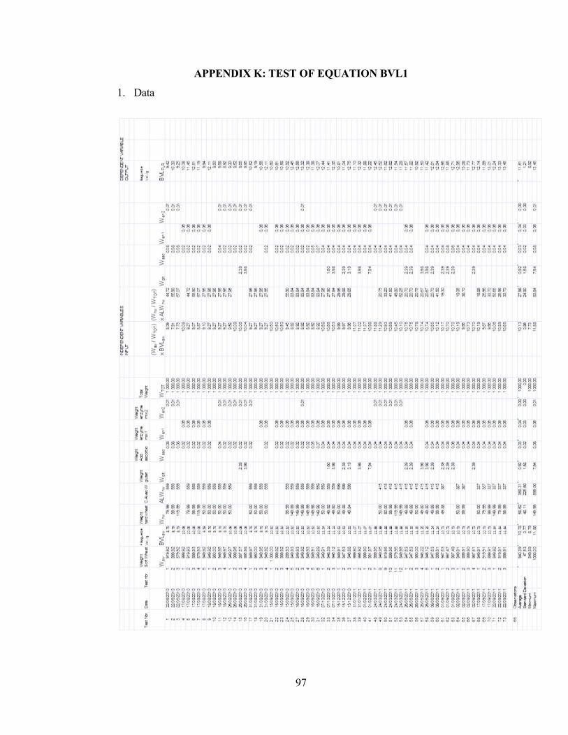
97

APPENDIX K: TEST OF EQUATION BVL1

1. Data

98


SUMMARY OUTPUT



R Square 0,654899391



Observations 66

ANOVA


Regression 6 61,83878472 10,30646412 18,66077268 4,99257E‐12

Residual 59 32,5860774 0,552306397

Total 65 94,42486212

Coefficients

Standard


Intercept ‐1,02368998 1,598446392 ‐0,640428096 0,524373888 ‐4,222173795 2,174793836 ‐3,694842608 1,647462649

(Wsw / WTOT) x BVLsw 1,048220541 0,152271909 6,883873391 4,25263E‐09 0,743525158 1,352915924 0,793760015 1,302681066

(Whw / WTOT) x ALWhw 0,029520273 0,005339277 5,528889854 7,70595E‐07 0,018836405 0,040204141 0,020597845 0,038442701

Wglt 0,015928725 0,065370127 0,243669784 0,808331866 ‐0,114876596 0,146734046 ‐0,093310839 0,125168289

Waac 6,930560558 5,513647052 1,25698299 0,213713261 ‐4,102221616 17,96334273 ‐2,283256614 16,14437773

Wen1 23,02090359 5,998494894 3,837779976 0,000305001 11,01794314 35,02386405 12,99686057 33,04494662

Wen2 15,09429886 31,34194498 0,481600579 0,63187128 ‐47,62078766 77,80938539 ‐37,28100703 67,46960475

99

APPENDIX L: TEST OF EQUATION BVL2

1. Data

100


SUMMARY OUTPUT



R Square 0,65844281



Observations 66

ANOVA


Regression 8 62,17337157 7,771671446 13,73534261 7,18822E‐11

Residual 57 32,25149055 0,565815624

Total 65 94,42486212

Coefficients

Standard


Intercept ‐1,155983662 1,627365011 ‐0,710340738 0,480389167 ‐4,414725861 2,102758536 ‐3,876984973 1,565017648

(Wsw / WTOT) x BVLsw 1,048789 0,1543427 6,79519667 6,97607E‐09 0,739723077 1,357854923 0,790723547 1,306854453

(Whw / WTOT) x ALWhw 0,037374935 0,011740049 3,183541703 0,002357669 0,013865893 0,060883976 0,017745234 0,057004635

‐((Whw / WTOT) x ALWhw)² 0,00010226 0,000134884 0,758136989 0,451492256 ‐0,00016784 0,000372361 ‐0,000123269 0,00032779

Wglt ‐0,004726989 0,142739632 ‐0,033116163 0,973697647 ‐0,29055817 0,281104192 ‐0,243391777 0,2339378

‐Wglt² ‐0,004964337 0,024562627 ‐0,20210937 0,840550849 ‐0,05415015 0,044221475 ‐0,04603376 0,036105085

Waac 6,954831844 5,615083137 1,238598196 0,22057102 ‐4,289178103 18,19884179 ‐2,433749375 16,34341306

Wen1 23,96187908 6,197020818 3,866677196 0,000285425 11,55255904 36,37119912 13,60028125 34,32347691

Wen2 18,59552486 32,10703875 0,579172841 0,564754516 ‐45,69771074 82,88876046 ‐35,08837147 72,27942118

101

APPENDIX M: QUALITY TESTS OF ACTUAL FLOURS

1. February 2011

FEBRUARY 2011

Date code Prot TCH W Vol.

04/02/11 1 10,8 354 243

04/02/11 2 10,6 347 248

04/02/11 3 10,6 361 252 12,18

05/02/11 1 10,9 372 235

05/02/11 2 11,1 385 241 12,12

07/02/11 1 10,9 378 224

07/02/11 2 11,0 381 222 12,67

08/02/11 1 10,9 370 256

08/02/11 2 11,1 368 245

08/02/11 3 11,2 377 235 12,24

09/02/11 1 11,0 372 232

09/02/11 2 11,0 372 225

09/02/11 3 11,1 381 236 12,57

10/02/11 1 10,9 384 230

10/02/11 2 11,0 371 238

10/02/11 3 11,2 376 223 12,57

11/02/11 1 10,8 368 234

11/02/11 2 10,9 377 246

11/02/11 3 11,0 377 239 13,43

12/02/11 1 10,8 354 240

12/02/11 2 10,9 362 233

12/02/11 3 10,9 355 224 12,29

14/02/11 1 11,0 349 278

14/02/11 2 11,0 352 278 12,09

Average 10,9 368 240 12,46

Standard deviation 0,2 12 15 0,42

n 24 24 24 9

3 Av‐(3std/n1/2) 10,8 361 231 12,04

3 Av+(3std/n1/2) 11,0 376 249 12,88

MODEL EQUATIONS 10,9 377 243 12,80

14,052

OK ERR OK OK

102

2. May 2011

MAY 2011


14/05/11 1 10,9 368 199

14/05/11 2 11,0 385 202

14/05/11 3 11,0 394 209 11,79

16/05/11 1 11,0 387 228 12,67

17/05/11 1 10,9 351 205

17/05/11 2 11,0 379 212 12,84

18/05/11 1 10,9 352 190

18/05/11 2 11,0 374 201

18/05/11 3 11,1 336 211 11,76

19/05/11 1 10,9 388 236

19/05/11 2 11,0 349 238

19/05/11 3 11,2 378 241 12,29

20/05/11 1 10,9 395 232

20/05/11 2 10,9 355 225

20/05/11 3 11,0 369 222 12,44

21/05/11 1 10,8 357 237

21/05/11 2 10,9 362 237

21/05/11 3 11,0 374 207 11,47

22/05/11 1 10,9 351 232

22/05/11 2 10,9 368 265

22/05/11 3 11,0 365 243 11,76

23/05/11 1 10,9 348 225

23/05/11 2 11,0 357 234 11,92

24/05/11 1 10,9 361 232

24/05/11 2 11,1 368 256 12,91

25/05/11 1 10,9 372 215

25/05/11 2 11,0 354 231 11,38

26/05/11 1 10,9 339 227

26/05/11 2 11,1 344 245 12,89

27/05/11 1 10,9 352 210

27/05/11 2 11,0 356 223 12,83

28/05/11 1 10,8 352 222

28/05/11 2 11,0 365 243 11,35

30/05/11 1 11,0 364 225 13,08

31/05/11 1 11,0 373 224

Average 11,0 364 225 12,23


n 35 35 35 15

3 Av‐(3std/n1/2) 10,9 356 217 11,74

3 Av+(3std/n1/2) 11,0 372 234 12,71


15,833

OK ERR OK ERR

103

3. August 2011

AUGUST 2011


23/08/11 1 11,1 361 234

23/08/11 2 11,1 358 241

23/08/11 3 11,1 367 248 12,34

24/08/11 1 11,1 349 227

24/08/11 2 11,2 354 241

24/08/11 3 11,4 370 265 12,20

25/08/11 1 11,2 357 238

25/08/11 2 11,2 354 238

25/08/11 3 11,3 351 259 12,59

26/08/11 1 11,2 353 236

26/08/11 2 11,2 367 226

26/08/11 3 11,4 363 238 12,51

27/08/11 1 11,2 390 282

27/08/11 2 11,3 377 231 12,32

29/08/11 1 11,4 387 266 12,83

31/08/11 1 11,0 375 262

31/08/11 2 11,2 364 254 11,88

01/09/11 1 11,1 384 264

01/09/11 2 11,2 376 264 12,99

02/09/11 1 11,2 373 234

02/09/11 2 11,3 376 232 12,26

03/09/11 1 11,2 375 224

03/09/11 2 11,4 346 267 11,82

05/09/11 1 11,3 361 233

05/09/11 2 11,4 329 242 12,48

06/09/11 1 11,0 358 250

06/09/11 2 11,2 374 231 12,12

07/09/11 1 11,0 357 229

07/09/11 2 11,1 372 228 12,20

08/09/11 1 10,8 362 226

08/09/11 2 11,0 362 243 12,32

09/09/11 1 10,8 357 252

09/09/11 2 10,9 361 265

09/09/11 3 11,0 356 223 12,20

10/09/11 1 10,8 367 235

10/09/11 2 11,0 366 241

10/09/11 3 11,1 346 247 12,17

12/09/11 1 10,9 366 244

12/09/11 2 11,0 384 261

12/09/11 3 11,1 381 246 12,20

13/09/11 1 11,0 354 240

13/09/11 2 11,1 368 246

13/09/11 3 11,1 358 262 12,83

14/09/11 1 10,9 361 230

14/09/11 2 11,0 358 263

14/09/11 3 11,2 354 260 12,32

15/09/11 1 11,0 349 249

15/09/11 2 10,9 352 250

15/09/11 3 11,2 348 260 12,20

16/09/11 1 10,8 376 235

16/09/11 2 10,8 372 209

16/09/11 3 11,0 364 229 11,81

17/09/11 1 10,8 362 255 12,73

19/09/11 1 11,0 346 261 12,71

20/09/11 1 10,6 350 240

20/09/11 2 10,8 351 244

20/09/11 3 10,9 345 240 12,20

21/09/11 1 10,8 352 246

21/09/11 2 10,8 342 219

21/09/11 3 11,0 346 242 12,67

22/09/11 1 10,8 339 221

22/09/11 2 10,9 351 227

22/09/11 3 11,1 348 244 12,22

23/09/11 1 10,8 360 228

23/09/11 2 10,9 365 281 12,93

24/09/11 1 10,9 332 237 12,33

26/09/11 1 10,9 363 238 12,26

Average 11,1 360 244 12,37


n 67 67 67 29

3 Av‐(3std/n1/2) 11,0 356 238 12,19

3 Av+(3std/n1/2) 11,1 365 249 12,54


14,536

OK OK OK ERR

104

4. February 2012

FEBRUARY 2012


01/02/12 1 11,3 349 274

01/02/12 2 11,0 345 242

01/02/12 3 11,1 348 236

01/02/12 4 11,2 347 256 12,55

01/02/12 5 11,3 337 293

02/02/12 1 11,4 337 272

02/02/12 2 11,4 339 279

02/02/12 3 11,3 348 256 12,59

02/02/12 4 11,2 343 283

03/02/12 1 11,4 340 278

03/02/12 2 11,4 344 265

03/02/12 3 11,3 346 239 12,61

06/02/12 1 11,5 347 275

06/02/12 2 11,5 347 275

06/02/12 3 11,3 338 286 12,98

07/02/12 1 11,4 340 239

07/02/12 2 11,4 353 304 13,18

08/02/12 1 11,3 352 273

08/02/12 2 11,3 345 286

08/02/12 3 11,3 355 252 12,92

09/02/12 1 11,3 339 279

09/02/12 2 11,3 341 255

09/02/12 3 11,3 361 307 13,06

10/02/12 1 11,3 347 267

10/02/12 2 11,4 355 254

10/02/12 3 11,3 368 306 13,07

11/02/12 1 11,2 351 267

11/02/12 2 11,3 345 262

11/02/12 3 11,2 357 279 13,25

11/02/12 4 11,2 357 279

14/02/12 1 11,3 347 293

14/02/12 2 11,5 351 281

14/02/12 3 11,2 349 300 12,96

15/02/12 1 11,2 347 291

15/02/12 2 11,3 336 260

15/02/12 3 11,2 342 295 13,83

16/02/12 1 11,1 329 291

16/02/12 2 11,2 351 260

16/02/12 3 11,2 341 254 13,13

Average 11,3 347 273 13,01


n 39 39 39 12

3 Av‐(3std/n1/2) 11,2 343 264 12,71

3 Av+(3std/n1/2) 11,3 350 282 13,31


15,131

ERR OK OK ERR

AN OPTIMIZATION MODEL: MINIMIZING FLOUR MILLERS’ COSTS …

Documents

Transcript of AN OPTIMIZATION MODEL: MINIMIZING FLOUR MILLERS’ COSTS …