An Introduction to the LS Dyna-R Smoothed Particle ...

13th International LS-DYNA Users Conference Session: Fluid Structure Interaction

1-1

5/20/2014

An Introduction to the LS-DYNA® Smoothed Particle Galerkin Method for Severe Deformation and Failure

Analyses in Solids

C. T. Wu1*, Y.Guo1 and W. Hu1 1 Livermore Software Technology Corporation

7374 Las Positas Road, Livermore, CA 94550, USA

Abstract This paper presents a new particle method in LS-DYNA for the severe deformation and failure analyses of solid mechanics problems. The new formulation is first established following a standard meshfree Galerkin approach for a solving of the partial differential equation of linear elastic problems. A smoothed displacement field is introduced to the Galerkin formulation and leads to a regularized smoothed strain approximation. The resultant smoothed/regularized strain formulation can be related to the residual-based stabilization method for the elimination of zero-energy modes in the conventional particle methods. The discretized system of equations are consistently derived within the meshfree Galerkin variational framework and integrated using a direct nodal integration scheme. The linear formulation is next extended to the large deformation and failure analyses of inelastic materials. In the severe deformation range, an adaptive Lagrangian or Eulerian kernel approach can be preformed to reset the reference configuration and maintain the injective deformation mapping at the particles. Several numerical benchmarks are provided to demonstrate the effectiveness and accuracy of the proposed method. Keywords: particle; convex approximation; nodal integration; inelastic

1. Introduction

Meshfree, or particle methods, offer many numerical advantages over the conventional finite

element and finite difference methods in modeling large deformation, moving discontinuity and immersed problems in solid and structural applications [1]. Those methods were also found to be very effective in reducing the volumetric locking and shear locking in the solid and structural analyses [3]. The earliest development in the meshfree methods was the Smoothed Particle Hydrodynamics (SPH) method. The foundation of the SPH method is the kernel estimate introduced by Monaghan [6]. In this method, partial differential equations are transformed into integral equations and the kernel estimate then provides the approximation to estimate the field variables at discrete particles. Since the functions are evaluated only at the particles, the use of a mesh is no longer required. The ability to handle severe deformations without the use of meshes in fluid-like motion allows the SPH method to be applied to problems that historically have been reserved for Eulerian approaches [7-8]. Nevertheless, a direct application of the SPH method to * Corresponding author. Tel: +1 925-2454529; Fax: +1 925-4492507. E-mail address: [email protected] (C. T. Wu).

Session: Fluid Structure Interaction 13th International LS-DYNA Users Conference

1-2

solid and structural analyses suffers from several numerical deficiencies, namely the lack of approximation consistency, tension instability, diffusion in material history information, presence of spurious or zero-energy modes and difficulty in enforcing the essential boundary conditions [9-10].

The Reproducing Kernel Particle method (RKPM) [10] introduced a correction function that restores the first-order consistency of the kernel approximation in the SPH method and improves the solution accuracy for finite domain problems. Tensile instability [12] is a major numerical defect in the SPH method that exhibits numerical fracture and artificial voids in the solid and structural applications. Tension instability was first identified by Swegle et al. [13] in a Von Neumann stability analysis and was later found to be related to the Eulerian kernels used in the Lagrangian description of motion [14]. A byproduct of Eulerian kernels in SPH is the diffusion problem in tracking the material history information during the deformation. Although an adoption of Lagrangian kernels can be used to alleviate the tension instability and reduce the diffusion problem [15], it suffers excessively from the intrinsic defects of purely Lagrangian methods and limits the magnitude of distortions in the severe deformation analysis. The presence of spurious or zero-energy modes in SPH or other Galerkin-based meshfree methods is mainly due to the rank instability caused by the under-integration of the weak forms inherent in the central difference formula from the nodal integration. Several meshfree nodal integration methods [16] have been developed to eliminate the spurious zero or near-singular modes due to the rank instability using the direct nodal integration scheme. Chen et al. [18] proposed a Stabilized Conforming Nodal Integration (SCNI) method in which a strain smoothing scheme was introduced as a stabilization process for the nodal integration. A common feature of the SPH stress point and the SCNI methods is their integration of the discretized system of equations over the background, or integration, cells, thus limiting their ability to model severe deformation problems.

The robustness and accuracy of the meshfree or particle methods in the solid and structural analyses are also greatly affected by their numerical treatments of the boundary conditions. Since the Kronecker-delta property does not hold in the conventional meshfree approximations such as the SPH kernel approximation, Moving Least-squares (MLS) or Reproducing Kernel (RK) approximations, special techniques [3] are needed to impose the constraint and the essential boundary conditions in the meshfree methods. Alternatively, several convex approximations were introduced [20] to simplify the essential boundary condition treatment in the meshfree methods. Meshfree convex approximations guarantee the unique solution inside a convex hull with a minimum distributed data set and possess the Kronecker-delta property at the boundaries, therefore avoid any special treatment on the essential boundaries. It has been shown [21] that the meshfree convex approximation exhibits smaller lagging phase and amplitude errors than the meshfree non-convex approximation in a full-discretization of the wave equation. Several meshfree and meshfree-enriched Galerkin formulations [22] using the meshfree convex approximation have been presented for the analyses of immersed composites, rubber-like materials in large deformation, and multi-scale acoustic waves.

This paper presents an alternative particle formulation [10] that provides a stable and accurate solution for problems in the solid mechanics applications. Since the formulation is derived based on a smoothed displacement field within the meshfree Galerkin variational framework and the discretized system of equations are integrated at the particles, we refer this formulation as the Smoothed Particle Galerkin (SPG) method. The reminder of the paper is outlined as follows: In the next section, we define the boundary-value problem of the linear elasticity and formulate the meshfree Galerkin method. In Section 3, we present a Smoothed Particle Galerkin formulation and its strain regularization. In Section 4, the Smoothed Particle Galerkin formulation is


1-3

extended to the large deformation analysis of inelastic materials with the adaptive Lagrangian or Eulerian kernel approach. Section 5 describes the SPG explicit dynamic formulation. The LS-DYNA input format is also provided in the same section. Several numerical examples are presented in Section 6 to illustrate the accuracy and robustness of the method. Final remarks are drawn in Section 7.

2. Preliminaries

To better illustrate the fundamental concept of the present method, we first consider the static

response of an elastic body under plain strain conditions. We assume the domain ℝ2 be a bounded polygon with the smooth boundary . Also, let u be the displacement and further assume that the Dirichlet boundary conditions are applied on D and the Neumann boundary

conditions are prescribed on N . For a prescribed body force ΩL2Xf , the governing

equilibrium equation and boundary conditions are written as

in Ω

on ;

on D

D N D NN

σ u f

u g

σ n t

(1)

where g is the prescribed displacement on D , t is the prescribed traction, n is the outward unit

normal to the boundary N and stands for the divergence operator. The infinitesimal strain

tensor uε is defined by

1

2s ε u u u u (2)

where is the gradient operator. In the case of linear isotropic elasticity, the Cauchy stress tensor σ and strain tensor ε have the following relationship

: 2 tr σ C ε u ε u ε u I (3)

where C is the fourth-order elasticity tensor and I is the identity tensor. The positive constants

and are the Lamé constants such that 21, with 210 and ,0 . The Lamé constants can be related to the Young’s modulus E and the Poisson ratio v by

vv

vE

v

E

211 ,

12

(4)

The variational form of this problem is to find the displacement

g 1 : on D u V v H v g such that for all Vu

: : 0N

s s d d d

u C u u f u t (5)

where the space 10 V H consists of the functions in the Sobolev space 1 H which

vanishes on the boundary in the sense of traces and is defined by

1: , Don V v v H v 0 (6)


1-4

By the Lax-Milgram theorem, there exists a unique solution gu V to the problem. Moreover, let g 2 u V H 2L f , 2

1 1= where D

g w w H , and 2=N

t w where 12 w H ,

we have the following elliptic regularity estimate for the linear elasticity posed in a convex domain with a polygonal boundary:

1 1 22 1 0 2 1C u u f w w (7)

where m

is the Sobolev norm of order m as defined in a standard way. The constant 1C in

Eq.(7) does not depend on and . For simplicity, we assume the homogenous Dirichlet boundary conditions in the following

derivation. The standard meshfree Galerkin method is then formulated on a finite dimensional subspace h V V employing the variational formulation of Eq. (5) to find hh Vu such that

: : 0 N

s h s h h h h hd d d

u C u u f u t u V (8)

3. A Smoothed Particle Galerkin Formulation for Linear Elasticity

This section describes the derivation of the smoothed particle Galerkin formulation for the analysis of linear elasticity problems using a direct nodal integration scheme. For a particle

distribution noted by an index set NP

IIIZ 1 X , we approximate the displacement field using the

meshfree approximation constructed by either the conventional meshfree approximation methods or the convex approximation methods to give

NP

1III

h Ψ XXuuXXu ˆ~ (9)

where NP is the total number of particles, and XIΨ , I=1,…NP can be considered as the shape

functions of the meshfree approximation for the displacement field Xuh . With the meshfree shape functions, we can define the corresponding finite-dimensional approximation space to be

XXV and : IIh ZIΨspan . In general, Iu~ is not the particle displacement and is

often referred to as the “generalized” displacement of particle I in the meshfree Galerkin method. Using Eq. (9), the particle displacement at particle I can be expressed by

I

NP

1JJIJI

h Ψ uuXXu ˆ~

(10)

where III Y,XX is the nodal coordinate of particle I. If the meshfree shape functions XIΨ are constructed using a convex approximation, then they have the Kronecker-delta property on the boundary, i.e. ˆ for I I I u u X . In this study, the first-order convex approximation is

constructed by the GMF method using the inverse tangent basis function and the cubic spline window function. Giving a convex hull Convex( IZ ) of the node set 2 NP1,I,Z II X defined by

NP

1IIIIII

NP

1IIII Z0,α1,α,ααZConvex XX (11)


1-5

the GMF method is used to construct a convex approximation of a given (smooth) function Xu in the form of Eq. (9) such that the shape function lI ZConvexΨ : satisfies the

following linear polynomial reproduction property

II

NP

II ZConvexΨ X XXX

1

(12)

With the meshfree convex approximation, we can also define a 10H -conforming subspace for

the approximation of the displacement field to be I0

IIh ZIΩ,Ψ suppΨ span:V . An

evaluation of the weak form in Eq. (8) using the meshfree approximation and the direct nodal integration scheme leads to the spurious, or zero-energy, modes. This is a consequence of the fact that the field variables and their derivatives are calculated at the same points such that an alternating field variable has a zero gradient at the particles [25]. The almost vanishing first derivatives at the nodes result in a discrete weak form that does not adequately reflect the strain energy and its contribution to the stiffness matrix is severely underestimated [16]. In order to eliminate the presence of the spurious or zero-energy modes caused by the direct nodal integration scheme, the smoothed particle Galerkin method introduces a smoothing of the displacement field defined by

dΩ;Ψ YuXYXu ˆ~ (13)

where Y denotes the position of the infinitesimal volume dΩ. The discrete form of Eq. (13)becomes

NP

1JJIJI Ψ uXu ˆ~ (14)

where IJΨ X~

, J=1,…NP are the displacement smoothing functions for particle I. It is assumed

that the displacement smoothing functions Ψ~

also satisfy the linear polynomial reproduction condition. In another words, the smoothed displacement field Xu equals to Xu for

homogeneous displacement states. For a sufficiently smoothed displacement field Xu , the

integral form in Eq.(13) can be expressed in terms of the gradients of Xu by expanding u X

into a Taylor series to yield

ˆ ˆ ˆ ˆ ˆ(2) (3)3(2) (2) (3)1 1

2! 3! u Y u X u X Y X u X Y X u X Y X (15)

where ( )n denotes the nth-order gradient operator and n denotes the nth-order inner product.

The symbol nξ designates the n factor dyadic product ξξξ for a vector ξ. Substituting Eq.(15) into Eq.(13) leads to the following smoothed displacement field in terms of the gradients

2(2)

(4)3(3)

ˆ ˆ

ˆ

ˆ

(2)

(3)

Ψ ; dΩ Ψ ; dΩ

1Ψ ; dΩ

2!1

Ψ ; dΩ O3!

u X Y X u X Y X u X Y - X

Y X u X Y - X

Y X u X Y - X Y X

(16)


1-6

Truncating the Taylor series in Eq.(16) after the quadratic term and using the linear polynomial reproduction condition of the displacement smoothing functions Ψ

~ leads to

ˆ ˆ

ˆ

ˆ ˆ

ˆ

ˆ

(2)2(2)

(2)2(2)

(2

Ψ ; dΩ Ψ ; dΩ

1Ψ ; dΩ

2!

Ψ ; dΩ Ψ ; dΩ Ψ ; dΩ

1Ψ ; dΩ

2!

Ψ ; dΩ

u X Y X u X Y X u X Y - X

Y X u X Y - X

u X Y X u X Y X Y X Y X

u X Y X Y - X

u X Y X

)

ˆ

ˆ ˆ

(2)2)

2(2

1Ψ ; dΩ

2!

u X Y X Y - X

u X u X η X

(17)

with dΩ;Ψ2!

1 (2)X-YXYXη~ defines the position dependent coefficients. In a nodal

integration, 2hI Xη that is proportional to a length squared where h denotes a characteristic

length scale of the discretization. Note that with the convex approximation, we have ˆ and for on I I I I η X 0 u X u X X . A modified weak form is obtained by neglecting

the higher-order gradient terms in strains to find hVuˆ , such that

hh la Vuuuu ˆ ˆˆ,ˆ (18)

where

ˆ ˆ ˆ ˆ ˆ ˆ, : : : :

ˆ ˆ ˆ ˆ , ,

(2) (2)h s s

h hstan stab

a d d

a a

u u u C u u C u

u u u u (19)

ˆ ˆ ˆ ˆ :N

2l d d d

u u f u t u η f (20)

where hstana is the standard bilinear form defined in Eq. (8) and

ˆ ˆ ˆ ˆ, : :

1ˆ ˆ ˆ: :

2

(2) (2)hstab

(2) (2) (2)

a d

u u u C u

u η u u η

(21)

defines the stabilized bilinear form which corresponds to the variation of the stabilized potential energy. The stabilization terms containing the first derivatives of the displacements are also omitted in Eq.(21) by considering their zero gradients at the particles. In the standard isotropic linear elastic case, coercivity of the bilinear form ,ha on hh VV follows immediately from one of the Korn’s inequalities to give


1-7

22 22

1 11 0 0 0

1

min

2 1 2

ˆ ˆ ˆ ˆ

ˆ ˆ ˆ ˆ , ,

ˆ ˆ ˆ , , , 0,

(2)s s

h hstan stab

h h

c c

ca a

c a c c

u u u u

u u u uC

u u u V

(22)

where min is the smallest eigenvalue of C. In other words, the stabilization term can be considered to enhance the coercivity of the formulation in the particle integration method. Using the Cauchy-Schwarz inequality and the first-order meshfree interpolation property [20] for the

displacement smoothing function Ψ~

, ,ha also can be bounded by

1/2 1/22 2

max 0 0

1/2 1/22 2

3 0 0

max 4 51 1 1 1

ˆ ˆ ˆ ˆ ˆ ˆ, : : : :

ˆ ˆ ˆ ˆ

ˆ ˆ ˆ ˆ

ˆ ˆ ˆ ˆ ,

(2) (2)h s s

3 4 5

a d d

d d

c h d h d

c c c ,c ,c

u v u C v u C v

C ε u ε v

ε u ε v

C u v u v ˆ ˆ h0 , u v V

(23)

where max is the largest eigenvalue of C. The third inequality is obtained using a simple triangle

inequality for the strain component of norm 0

ˆˆ uε defined in L2 space [22]. Since Eq. (21)

includes non-zero second derivatives of the displacements, it serves as a stabilization term and appears like the residual-based stabilization method [16] for the nodal integration in the Element-Free Galerkin method. The numerical evaluation of Eq. (21) using a direct nodal integration results in a symmetric stiffness matrix. Compared to the residual-based stabilization method, the stabilization parameter in Eq. (21) is derived in a consistent manner without additional prescription of its value. However, the integration of Eq. (21) involves the second derivatives and is expensive for the assembly of linear systems in multi-dimensional problems. In this study, an alternative way to implement the smoothed displacement field in Eq. (8) without the involvement of second-order derivatives in the shape functions is introduced. This is to use the integral form in Eq. (13) instead of the gradient form in Eq. (17). By substituting Eq. (10) into Eq.(14), we have the discrete smoothed displacement field evaluated at the particles by

NP

1KKIK

NP

1K

NP

1JKIJJK

NP

1J

NP

1KKJKIJ

NP

1JJIJI ΨΨΨΨΨ

uX

uXXuXXuXu

~

~~~~ˆ~

(24)

where the smoothed meshfree shape function IK X is defined by

NP

1JIJJKIK ΨΨ XXX

~: (25)

Now the relationships between the different nodal position systems can be defined through Eqs. (10), (14) and (24), and are shown in Figure 1.


1-8

Figure 1: The relationships between different nodal position systems.

The smoothed meshfree shape function constructed by the meshfree convex approximation continues to satisfy the Kronecker-delta property on the boundary,

gKKI

NP

1JIJJKIK ΨΨ

XXXX ~ (26)

Using Eq. (9), we have the admissible test functions for the variation equation obtained by

NP

1III

h Ψ uXXu ~ (27)

By introducing the displacement and strain approximations into Eq. (8), the discrete governing equation is integrated using a direct nodal integration to give

extTT δδ fUUKU~~~ (28)

0

1KK

NP

KJK

TIJ

TIIJ VdΩ XCBXBCBBK

(29)

KK

NB

KKIKK

NP

KKIΓ II

extI LΨVΨdΓΨdΨ

N

XtXXfXtff

1

0

1

(30)

where 0KV denotes the initial volume of particle K. In Eq. (30) NB denotes the number of

boundary nodes and Lk is the length associated with the boundary particle along the global boundary. To explore the concept of the method as well as to improve computational efficiency,

we simply consider XX II ΨΨ ~ in this study. From Eq. (14), we have

NP

1KKIK

NP

1K

NP

1JKIJJKI ΨΨ uXuXXu ~~ (31)

or in matrix form

UAU~ or UAU -1~

(32)


1-9

where vector NPuuuU ~,,~,~~21 contains the problem unknowns for the generalized

nodal displacements. A is a transformation matrix defined by

IXXIXA

NP

1KKJIKIJIJ ΨΨ (33)

Substituting Eq. (32) into the variation form of Eq. (28) leads to the following discrete equation to be solved for the linear elastic analysis

extTT fAUKAA --1- (34)

or equivalently

extTT fAUKA -- ~ (35)

4. Large Deformation Analysis for Inelastic Material and Adaptive

Lagrangian/Eulerian Kernel Approach

The smoothed meshfree Galerkin formulation presented in the previous section is now extended to the nonlinear analysis of plastic materials. In light of the rate constitutive equations and the derivatives with respect to the spatial coordinates, it is advantageous to use the variational formulation of the equation of motion in terms of the updated Lagrangian formulation in the following derivation.

In a quasi-static problem, the variational formulation of the updated Lagrangian formulation with reference to the current configuration x is expressed in an index form by

0 dtudfud

Nxxiiiiijij (36)

where σij is the Cauchy stress defined at the current configuration. We also have iii uXx that

relates the spatial coordinate x to the reference coordinate X. Linearizing of Eq. (36) leads to the iterative equations

,, dtudfuduTudC

Nxxxiiiilkijkljiklijklij (37)

where *lgijkl

aijklijkl CCC (38)

iljkjlikikjljkiljlijkl ikC 2

1* (39)

jlikijklT (40)

Cijkl is the material tangent response tensor, lgaijklC is the algorithmic tangent response tensor for

the infinitesimal plasticity. Substituting the discrete meshfree approximation in Eq. (24) and its variation into Eq. (37) leads to the discrete iterative equation given by

v1n

Tv

nv

1nT δδ

RUUKU~~~ 1

1 (41)


1-10

The notation vn 1 represents the function to be computed in the v-th iteration during (n+1)th

time incremental step. Using Eq. (32), the discrete iterative equation can be written in the smoothed nodal position system as in the linear analysis to yield

v1n

-Tv

nv

1n-T

RAUAKA

1

11 (42)

or equivalently

v1n

T-v

nv

1nT-

RAUKA1

1

~ (43)

As Lagrangian simulation proceeds, an adaptive Lagrangian/Eulerian kernel scheme is performed frequently to avoid the negative Jacobian in the Lagrangian calculation. In each adaptive step material quantities are computed at the particles without the usage of any background cells. Since the adaptive Lagrangian/Eulerian kernel approach does not involve remeshing and the particle computation is evaluated node-wisely, the material quantities at all particles are maintained in the Lagrangian setting and thus require no remap procedures. If we denote the variables before and after each adaptive time step to be superscripted with “–“and “+” respectively, the derivatives of the material meshfree shape functions with respect to the spatial coordinates right before (k+1)-th adaptive time step can be expressed by

1

1

k

jikj

Ikj

kj

kj

1kI

1ki

1kI1k

iI, fx

-Ψ

x

x

x

-Ψ

x

-Ψ-Ψxx

x (44)

where 1

1

kj

kjk

ji x

xf defines the inverse of the incremental deformation gradient from k-th

adaptive time step. At (k+1)-th adaptive time step, the new derivatives of the material meshfree shape functions becomes

i

1kI1k

iI, x

ΨΨ

x

x (45)

5. Explicit Dynamic Formulation and LS-DYNA Input Format

5.1 Explicit dynamic formulation

The explicit dynamic version of the smoothed particle Galerkin formulation can be easily obtained by considering the inertial effect and following the previous quasi-static derivation to yield

int1 ffAUMAA ext-T-T (46)

or equivalently

int~ffAUMA extT-T- (47)


1-11

where U and U~

contain the vector of particle accelerations evaluated in the smoothed nodal position system and generalized nodal position system, respectively. M is the consistent mass matrix given by

IXXM 00

1NNJ

NP

NNIIJ VΨΨ

(48)

where 0 is the initial density. Eq. (46) also can be rewritten as

intffAUM ext-T (49)

with 1 MAAM -T defines a smoothed consist mass matrix. In an explicit dynamic analysis, a row-sum mass matrix is usually considered which is only computed once without involving the matrix inversion at each time step. The smoothed consist mass matrix is now replaced by the row-sum mass matrix RSM to give

NP

JMLKM

TIK

NP

JIJ

RSI

1AMAMM (50)

Since no remap procedures are considered in the adaptive Lagrangian kernel scheme, the particle mass is taken to be the same during the explicit dynamics analysis. The current particle volume required for the calculation of the internal force is updated according to the continuity equation given by

00I

II VV

(51)

NP

JIJJIII

I Ψdt

d

1,

~~ xuu x

(52)

5.2 LS-DYNA input keyword

The new particle formulation is assigned an element type of 47 and can be accessed with an option of _SPG in the *SECTION_SOLID keyword card. It is implemented in such a way that one can easily take a finite element model and change some parts into SPG particles.

The input format is as follows:

*SECTION_SOLID_SPG

Card1 1 2 3 4 5 6 7 8

Variable SECID ELFORM AET

Type I I I

Default

The SPG method is selected by setting ELFORM to 47, and two optional input cards are defined to obtain additional input parameters from the user:


1-12

Card2 1 2 3 4 5 6 7 8

Variable DX DY DZ ISPLINE IDISC LSCALE SMSTEP SWTIME

Type F F F I I F I F

Default 1.5 1.5 1.5 0 0

Card3 1 2 3 4 5 6 7 8

Variable Others

Type I

Default 0

The variables are described as below:

VARIABLE DESCRIPTION

SECID Section ID.

ELFORM Element formulation options. Set to 47 to active SPG method.

DX, DY, DZ Normalized dilation parameters of the kernel functions in X, Y and Z directions.

ISPLINE Option for kernel functions. EQ.0: Cubic spline function (default). EQ.1: Quadratic spline function. EQ.2: Cubic spline function with circular shape.

IDISC Type of discretization. EQ.0: Moving least-square (default). EQ.1: Convex approximation.

LSCALE Length scale for displacement regularization.

SMSTEP Interval of time steps to conduct displacement regularization.

SWTIME Time to switch from adaptive Lagrangian kernel to Eulerian kernel.

Others Cards 3 leaves to further developments in material failure/damage analyses.

For the full description of the keyword *SECTION_SOLID, please refer to the LS-DYNA keyword users’ manual.

6. Numerical Examples

6.1 Implicit analysis for radial bushing problem

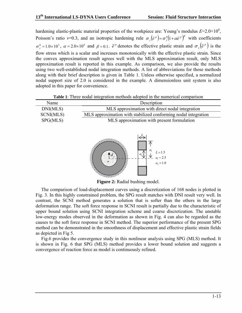
This example is analyzed to identify the applicability of the proposed method to highly constrained problem using implicit version of SPG method. The radial metal bushing model in plain strain condition, as shown in Fig. 2, is studied, where the outer surface is fixed, and the inner surface sticks with an un-deformed core moving along vertical direction. The strain-


1-13

hardening elastic-plastic material properties of the workpiece are: Young’s modulus E=2.0×106,

Poisson’s ratio v=0.3, and an isotropic hardening rule py

py ee 10 with coefficients

30 100.1 y , 4100.2 and 1.0 . pe denotes the effective plastic strain and py e is the

flow stress which is a scalar and increases monotonically with the effective plastic strain. Since the convex approximation result agrees well with the MLS approximation result, only MLS approximation result is reported in this example. As comparison, we also provide the results using two well-established nodal integration methods. A list of abbreviations for those methods along with their brief description is given in Table 1. Unless otherwise specified, a normalized nodal support size of 2.0 is considered in the example. A dimensionless unit system is also adopted in this paper for convenience.

Table 1: Three nodal integration methods adopted in the numerical comparison

Name Description DNI(MLS) MLS approximation with direct nodal integration SCNI(MLS) MLS approximation with stabilized conforming nodal integration SPG(MLS) MLS approximation with present formulation

Figure 2: Radial bushing model.

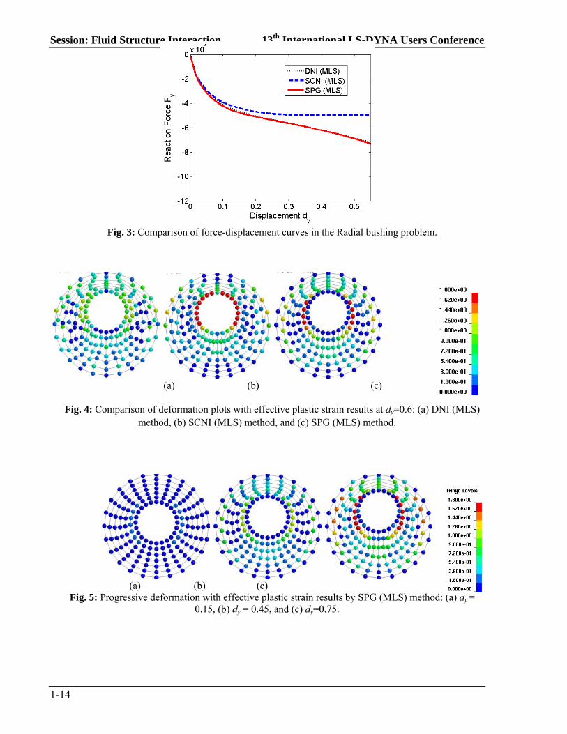
The comparison of load-displacement curves using a discretization of 168 nodes is plotted in Fig. 3. In this highly constrained problem, the SPG result matches with DNI result very well. In contrast, the SCNI method generates a solution that is softer than the others in the large deformation range. The soft force response in SCNI result is partially due to the characteristic of upper bound solution using SCNI integration scheme and coarse discretization. The unstable low-energy modes observed in the deformation as shown in Fig. 4 can also be regarded as the causes to the soft force response in SCNI method. The superior performance of the present SPG method can be demonstrated in the smoothness of displacement and effective plastic strain fields as depicted in Fig 5.

Fig.6 provides the convergence study in this nonlinear analysis using SPG (MLS) method. It is shown in Fig. 6 that SPG (MLS) method provides a lower bound solution and suggests a convergence of reaction force as model is continuously refined.

e1

2

1.5

2.5

1.0

L

a

a

2a1a

L

yd


1-14

Fig. 3: Comparison of force-displacement curves in the Radial bushing problem.

(a) (b) (c)

Fig. 4: Comparison of deformation plots with effective plastic strain results at dy=0.6: (a) DNI (MLS) method, (b) SCNI (MLS) method, and (c) SPG (MLS) method.

(a) (b) (c)

Fig. 5: Progressive deformation with effective plastic strain results by SPG (MLS) method: (a) dy = 0.15, (b) dy = 0.45, and (c) dy=0.75.


1-15

Fig. 6: Convergence study of implicit SPG (MLS) using four discretization refinements.

6.2 3D punch problem

The large deformation problem is studied next in the Prandtl’s punch problem using the explicit dynamic analysis. The model is shown in Fig. 7 which consists of a block of size 4×2×1 punched by a rigid, frictionless and flat plate with a vertical velocity of 2.0zv . The metal block is assumed elastic and the material properties are: Young’s modulus E=6.9×104, Poisson’s ratio v=0.3 and density 3

0 2.7 10 .

Figure 7: Prandtl’s punch model. Figure 8: SPG model for punch problem.

The elastic block is discretized by 21×11×5 uniformly distributed particles as shown in Fig. 8. Cubic spline kernel function with a normalized dilation parameter of 1.6 in X, Y and Z directions is used in the computation. The problem is simulated using both the adaptive Lagrangian kernel approach and Eulerian kernel approach.

Fig. 9 shows the comparison of the deformation plots between the adaptive Lagrangian kernel and Eulerian kernel approach. In the small deformation range, both approaches give almost identical results. However, when the deformation approaches to the large range, they behave quite differently. With the Eulerian kernel, the particles close to the edges of the impacting plate start to lose interaction with each other between t=0.3 and 0.4. This phenomenon leads to a numerical fracture similar to that of tensile instability [12-13] in SPH method and should be avoided. On the other hand, the Lagrangian kernel approach yields smooth and continuous deformation without numerical fracture. To generate a realistic result and prevent any numerical

zv


1-16

fracture, a physical-based failure criterion should be employed to both approaches for the consideration in material failure analysis.

It is interesting to show how stable the proposed SPG method is for the 3D large deformation problem. There is no bulk viscosity added in the numerical scheme for this elastic material problem and the computation is finished without shooting nodes or unstable modes.

Fig. 9: Progressive deformation with effective von-Mises stress.

t=0.2

t=0.4

t=0.6

t=0.8

(a) Adaptive Lagrangian (b) Eulerian


1-17

6.3 Plate impacted by a rigid ball The third benchmark problem is a circular plate impacted by a rigid ball, as shown in Fig. 10.

The plate has a radius of 20 and a thickness of 5 and is consisted of an elastic-perfectly plastic material with material properties of density 3

0 7.85 10 , Young’s modulus E=2.0×105,

Poisson’s ratio v=0.3 and yield stress 22.0 10y . The rigid ball has a radius of 5 and an impact

speed of 600.0.

Figure 10: Plate impact by a ball. Figure 11: Particle discretization of the plate.

The plate is modeled by 25721 particles as shown in Fig. 11. Cubic spline kernel function

with a normalized dilation parameter of 1.6 in X, Y and Z directions is adopted in the computation. To avoid any numerical fracture, the simulation is conducted with the adaptive Lagrangian kernel approach.

The progressive deformation of the plate is plotted in Fig. 14, together with the contours of the effective plastic strain. The results show that the proposed SPG method can handle large deformation with ease. Similar to the previous example, there is no shooting nodes or spurious zero-energy modes observed in the severe deformation range.

The time history of the velocity of the impacting ball and the time history of the impact force are displayed in Figures (12) and (13).

Figure 12: Time history of ball velocity. Figure 13: Time history of impact force.


1-18

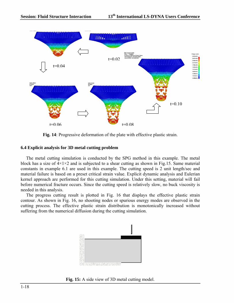
Fig. 14: Progressive deformation of the plate with effective plastic strain.

6.4 Explicit analysis for 3D metal cutting problem

The metal cutting simulation is conducted by the SPG method in this example. The metal block has a size of 4×1×2 and is subjected to a shear cutting as shown in Fig.15. Same material constants in example 6.1 are used in this example. The cutting speed is 2 unit length/sec and material failure is based on a preset critical strain value. Explicit dynamic analysis and Eulerian kernel approach are performed for this cutting simulation. Under this setting, material will fail before numerical fracture occurs. Since the cutting speed is relatively slow, no buck viscosity is needed in this analysis.

The progress cutting result is plotted in Fig. 16 that displays the effective plastic strain contour. As shown in Fig. 16, no shooting nodes or spurious energy modes are observed in the cutting process. The effective plastic strain distribution is monotonically increased without suffering from the numerical diffusion during the cutting simulation.

Fig. 15: A side view of 3D metal cutting model.

t=0.02

t=0.04

t=0.06 t=0.08

t=0.10


1-19

Fig. 16: Progress cutting history plots in effective plastic strain contour.

7. Conclusion

A new particle method is developed for the large inelastic deformation and failure analyses in solid mechanics applications. The present particle method is intimately related to the residual-based stabilization method for the elimination of zero-energy modes in conventional particle methods. No numerical viscosity and artificial control parameters are involved in the present formulation for the stabilization. The numerical results in quasi-static analyses justify the applicability of the present method for the large inelastic deformation analyses. A combination of explicit dynamic formulation and adaptive Lagrangian/Eulerian kernel approach helps advance the simulation to the severe inelastic deformation range. The method also could be a promising alternative for the simulation of impact and penetration problems involving material failure. Its extension to shell formulation is under investigation and will be reported in the near future.

References [1] S. Li, W.K. Liu, Meshfree Particle Method, Springer, Berlin 2004. [2] C.T. Wu, Y. Guo, E. Askari, Numerical modeling of composite solids using an immersed

meshfree Galerkin method, Composites B 45 (2013) 1397-1413. [3] J.S. Chen, C. Pan, C.T. Wu, W.K. Liu, Reproducing kernel particle methods for large

deformation analysis of non-linear structures, Comput. Methods Appl. Mech. Eng. 139 (1996) 195-227.

[4] J. Bonet, S. Kilasegaram, Correction and stabilization of smooth particle hydrodynamics methods with applications in metal forming simulations, Int. J. Numer. Methods Eng. 47 (2000) 1189-1214.

[5] C. Peco, A. Rosolen, M. Arroyo, “An adaptive meshfree method for phase-field models of biomembranes. Part II: A Lagrangian approach for membranes in viscous fluids, J. Comput. Phys. 249 (2013) 320-336.

[6] J.J. Monaghan, An introduction to SPH, Comput. Phys. Commun. 48 (1988) 89-96.


1-20

[7] E.S. Lee, C. Moulinec, R. Xu, D. Violeau, Comparisons of weakly compressible and truly incompressible algorithms for the SPH mesfree particle method, J. Comput. Phys. 227 (2008) 8417-8436.

[8] D. Violeau, Fluid Mechanics and the SPH method: Theory and Applications, Oxford University Press, Oxford, 2012.

[9] L.D. Libersky, A.G. Petscheck, T.C. Carney, J.R. Hipp, F.A. Allahadai, High strength Lagrangian hydrodynamics, J. Comput. Phys. 109 (1993) 67-75.

[10] C. T. Wu, W. Hu, M. Koishi, A smoothed particle Galerkin formulation for stabilzied large deformation analyses of non-linear continua, submitted to Journal of Computational Physics (2014).

[11] W.K. Liu, S. Jun, Y.F. Zhang, Y. F. Reproducing kernel particle methods, Int. J. Numer. Methods Fluids 20 (1995) 1081-1106.

[12] P.W. Randles, L.D. Libersky, Recent improvements in SPH modeling of hypervelocity impact, Int. J. Impact Eng. 48 (2000) 1445-1462.

[13] J.W. Swegle, D.L. Hicks, S.W. Attaway, Smoothed particle hydrodynamics stabiliy analysis, J. Comput. Phys. 116 (1995)123-134.

[14] T. Belytschko, Y. Guo, W.K. Liu, S.P. Xiao, A unified stability analysis ofmeshless particle methods, Int. J. Numer. Methods. Eng. 48 (2000) 1359-1400.

[15] T. Rabczuk, T. Belytschko, S.P. Xiao, Stable particle methods based on Lagrangian Kernels, Comput. Methods Appl. Mech. Eng. 193 (2004) 1035-1063.

[16] S. Beissel, T. Belytschko, Nodal integration of the element-free Galerkin method, Comput. Methods Appl. Mech. Eng. 139 (1996) 49-74.

[17] E. Oñate, F. Perazzo, J. Miquel, A finite point method for elasticity problems, Comput. Struct. 79 (2001) 2151- 2163.

[18] J.S. Chen, C.T. Wu, S. Yoon, Y. You, A stabilized conforming nodal integration for Galerkin meshfree methods, Int. J. Numer. Methods Eng. 50 (2001) 435-466.

[19] H.P. Wang, C.T. Wu, Y. Guo, M. Botkin, A Coupled Meshfree/finite Element Method for Automotive Crashworthiness Simulations, Int. J. Impact Eng. 36 (2009) 1210-1222.

[20] C.T. Wu, C.K. Park, J.S. Chen, A generalized approximation for the meshfree analysis of solids, Int. J. Numer. Methods Engrg. 85 (2011) 693-722.

[21] C.K. Park, C.T. Wu, C.D. Kan, On the analysis of dispersion property and stable time step in meshfree method using generalized meshfree approximation, Finite Elem. Anal. Des. 47 (2011) 683-697.

[22] C.T. Wu, W. Hu, Meshfree-enriched simplex elements with strain smoothing for the finite element analysis of compressible and nearly incompressible solids, Comput. Methods Appl. Mech. Eng. 200 (2011) 2991-3010.

[23] C.T. Wu, M. Koishi, Three-dimensional meshfree-enriched finite element formulation for micromechanical hyperelastic modeling of particulate rubber composites, Int. J. Numer. Methods Eng. 91 (2012) 1137-1157.

[24] C.T. Wu, W. Hu, Multi-scale finite element analysis of acoustic waves using global residual-free meshfree enrichments, Interact. Multiscale Mech., 6 (2013) 83-105.

[25] R. Vignjevic, J. Campbell, L.D. Libersky, A treatment of zero-energy modes in the smoothed particle hydrodynamics method, Comput. Methods Appl. Mech. Eng. 184 (2000) 67-85.

[26] J.C. Simo, T.J.R. Hughes, Computational Inelasticity, Springer, New York, 2000. [27] LS-DYNA User’s Manual, Livermore Software Technology Corporation, Livermore, USA,

2013.

An Introduction to the LS Dyna-R Smoothed Particle ...

Documents

Transcript of An Introduction to the LS Dyna-R Smoothed Particle ...