HAL Id: hal-03163631https://hal.archives-ouvertes.fr/hal-03163631

Submitted on 20 Aug 2021

HAL is a multi-disciplinary open accessarchive for the deposit and dissemination of sci-entific research documents, whether they are pub-lished or not. The documents may come fromteaching and research institutions in France orabroad, or from public or private research centers.

L’archive ouverte pluridisciplinaire HAL, estdestinée au dépôt et à la diffusion de documentsscientifiques de niveau recherche, publiés ou non,émanant des établissements d’enseignement et derecherche français ou étrangers, des laboratoirespublics ou privés.

An EWMA signed ranks control chart with reliable runlength performances

Theodoros Perdikis, Stelios Psarakis, Philippe Castagliola, Petros Maravelakis

To cite this version:Theodoros Perdikis, Stelios Psarakis, Philippe Castagliola, Petros Maravelakis. An EWMA signedranks control chart with reliable run length performances. Quality and Reliability Engineering Inter-national, Wiley, 2021, 37 (3), pp.1266-1284. �10.1002/qre.2795�. �hal-03163631�

An EWMA Signed Ranks Control Chart

with Reliable Run Length Performances

Theodoros Perdikis1, Stelios Psarakis∗1,Philippe Castagliola2, and Petros E. Maravelakis3

1Department of Statistics & Laboratory of Statistical Methodology,Athens University of Economics and Business Athens, Greece

2Universite de Nantes & LS2N UMR CNRS 6004, Nantes, France3Department of Business Administration, University of Piraeus,

Piraeus, Greece

August 20, 2021

Abstract

During the design phase of a control chart, the determination of itsexact Run Length properties plays a vital role for its optimal operation.Markov chain or integral equation methods have been extensively ap-plied in the design phase of conventional control charts. However, fordistribution-free schemes, due to the discrete nature of the statistics be-ing used (such as the Sign or the Wilcoxon Signed Rank statistics, forinstance), it is impossible to accurately compute their Run Length prop-erties. In this work, a modified distribution-free Phase II EWMA-typechart based on the Wilcoxon Signed Rank statistic is considered and itsexact Run Length properties are discussed. A continuous transformationof the Wilcoxon Signed Rank statistic, combined with the classical MarkovChain method, is used for the determination of the Average Run Lengthin the in- and out-of control cases. Moreover, its exact performance isderived without any knowledge of the distribution of sample observations.Finally, an illustrative example is provided showing the practical imple-mentation of our proposed chart.

Keywords:Nonparametric control chart; Wilcoxon signed rank statistic;Markovchain; EWMA control chart.

1 Introduction

SPM (Statistical Process Monitoring) techniques are of high importance formanufacturing and non-manufacturing applications as they aim to identify thepresence of possible assignable causes in processes. Control charts are one ofthe major tools of SPM. They are on-line process monitoring techniques whose

∗psarakis@aueb.gr(corresponding author)

1

purpose is to detect shifts in processes as fast as possible. One of the most com-monly used type of control chart is the Shewhart-type control chart (see She-whart 1). A significant improvement in charting techniques was the introductionof memory-type methods like the EWMA (Exponentially Weighted Moving Av-erage) by Roberts 2 and the CUSUM (Cumulative Sum) by Page 3 . It is wellknown that Shewhart-type control charts are preferable in cases where largemean shifts need to be detected. On the other hand, EWMA and CUSUMschemes are able to detect small to moderate shifts in processes, faster thanconventional standard control charts, due to the fact that, at each samplingpoint, they take into account previous measurements.

In general, during the design phase of a measurement control chart, its designparameters are obtained based on the assumption that the observations, col-lected over time, are normally distributed random variables or, at least, theyfollow some known distribution. However, in practice, this assumption is com-monly violated, since the underlying distribution of the characteristic to bemonitored is generally unknown. As a result, a new class of monitoring schemescalled distribution-free (or nonparametric) control schemes has been introducedinto the literature. For nonparametric control charts, the chart’s design param-eters as well as the Run Length properties are derived based on the distributionof the corresponding nonparametretric statistics which are used (such us theSign or the Wilcoxon Signed Rank statistics) with only a minimal knowledgeof the form of the underlying distribution for the characteristic to be moni-tored. For a comprehensive overview of the literature regarding the design andoperations of several univariate and multivariate nonparametric control chartsthe reader is advised to refer to Chakraborti et al. 4 , Qiu 5 , Chakraborti andGraham 6 . Concerning distribution-free EWMA control charts, two of the mostcommonly used nonparametric statistics that have been used and presented intothe literature are the Sign statistic (Amin and Searcy 7 , Graham et al. 8 , Yanget al. 9 , Aslam et al. 10 , Riaz 11 , Lu 12 , Haq 13) and the Wilcoxon Signed Rank orRank-Sum statistics (Li et al. 14 , Graham et al. 15 , Chakraborty et al. 16 , Abidet al. 17). Additionally, recent developments of distribution- free EWMA-typeschemes can be found at Raza et al. 18 , Alevizakos et al. 19 , Mabude et al. 20 .

The use of reliable metrics that can efficiently measure the performance of acontrol scheme plays a vital role in its design phase. One of the most widelyused technique is to examine the performance of a control chart by evaluating itsin- and out-of- control RL (Run Length) properties such as the ARL (AverageRun Length), SDRL (Standard Deviation Run Length) or quantile-type metricslike the MRL (Median Run Length) or the RL0.95 (0.95-quantile of the RL). ForEWMA and CUSUM-type schemes their RL properties are often obtained byusing the Markov Chain approach of Brook and Evans 21 which is based on thediscretization of the control limits interval into sub-intervals. It should be notedthat, regarding the design phase of an EWMA-type control chart a proper com-putation of its RL properties is essential. Specifically, for the determination ofthe design parameters λ (smoothing parameter) and K (control limit parame-ter) of an EWMA-type chart, a searching algorithm needs to be conducted, fora particular shift in the process, in order to find the optimal pair (λ∗,K∗) whichminimizes the out-of-control ARL, under the constraint ARL = ARL0 whereARL0 is some predefined value for the in-control ARL. In the case of measure-

2

ment data (usually assuming normality) as the number of sub-intervals increasesthe method proposed by Brook and Evans 21 tends to give reliable approxima-tions of the chart’s RL properties. However, in a nonparametric context, dueto the discrete nature of the statistics that is being used (for instance, the Signor Wilcoxon Signed Rank statistics), it is not feasible to exactly compute thein- (ARL0) and out-of-control (ARL1) ARL by using this approach (see Weiß 22

for instance). As it will be shown in the rest of the paper, the correspondingARL values are actually highly affected by the number of sub-intervals. Asa consequence, robust methodologies are essential for the proper computationof its RL properties. Castagliola et al. 23 based on the approach of Rakitziset al. 24 introduced a new class of distribution-free EWMA-type chart for countdata (CEWMA SN chart) in which a proper discrete Markov-chain approachwas used for the determination of the ARL for the in- and out-of control cases.Tang et al. 25 using the same discrete Markov method extended the CEWMASN chart by adding an adaptive feature in the smoothing parameter. Recently,Wu et al. 26 proposed a distribution-free EWMA-TBEA (Time Between Eventsand Amplitude) control chart where they introduced a new approach called asthe “continuousify” method in which the values of the initial discrete randomvariables are transformed into continuous ones based on weighted Gaussian Ker-nels. As a result, since the Markov chain of Brook and Evans 21 performs wellin the case of continuous random variables, Wu et al. 26 showed that the abovemethod yields robust results without the need of setting large values for thenumber sub-intervals used in the Markov chain. In this paper, based on theapproach of Wu et al. 26 we will introduce a distribution-free one-sided EWMAcontrol chart based on the Wilcoxon Signed Rank statistic with robust ARLresults regardless of the underlying distribution of the observations. It shouldbe noted that, this work aims to provide a methodology which guarantees stableresults in the chart’s RL properties.

The paper is organised as follows: In Section 2, a modified version of the non-parametric EWMA chart based on the Wilcoxon Signed Rank statistic proposedby Graham et al. 15 (denoted as the WSR EWMA chart) is proposed. More-over, an extension of the former control chart (denoted as the C-WSR EWMAchart) is presented in which the Gaussian Kernel estimation approach of Wuet al. 26 is used. In Section 3, a numerical analysis is conducted concerningthe robustness of the “continuousify” method and optimal design parameters(λ∗,K∗) are obtained under several shifts and sample sizes. Additionally, theefficiency of the “continuousify” method is examined for several Kernel densityfunctions. In Section 4 an illustrative example is discussed to show the practicalimplementation of the operation of our proposed chart. Finally, in Section 5,some concluding remarks and suggestions for future works are discussed.

2 The distribution free one-sided WSR EWMAchart

Graham et al. 15 introduced a new nonparametric two-sided EWMA chart basedon the Wilcoxon Signed Rank statistic (NPEWMA-SR chart). Using the Markov-Chain approach of Brook and Evans 21 they obtained its optimal design param-

3

eters and they examined its out-of-control performance under several symmet-ric distributions. In this current work, we present a modified version of theNPEWMA-SR chart, providing its Run Length properties for both in- and out-of-control conditions regardless of the observations’ underlying distribution. Wewill only focus on the design of an EWMA scheme capable of detecting increasesin the product’s characteristic. As mentioned above, this paper does not aimto investigate the performance of a new EWMA-type scheme based on SignedRanks but to present an improved and efficient approach to compute its RunLength properties. In this Section, a brief review of the Wilcoxon Signed Rankstatistic will be firstly presented and then our proposed modified version of theEWMA control chart based on signed ranks will be introduced.

2.1 Theoretical background of the Wilcoxon Signed Rankstatistic

The Wilcoxon Signed Rank test statistic is one of the most commonly usednonparametric technique for testing hypotheses about a location parameter, θ0,of a symmetric continuous distribution. Suppose that at each sampling pointt = 1, 2, . . . a subgroup {Xt,1, Xt,2, . . . , Xt,n} of size n is collected following anunknown continuous symmetric distribution with c.d.f. (cumulative distributionfunction) FX(x|θ) where θ is the location parameter to be monitored (assumedas known). With respect to the Phase II implementation of the control chart,when the process is in-control, assuming θ as the median of the process we havethat P(Xt,j > θ0|θ = θ0) = P(Xt,j < θ0|θ = θ0) = p0 = 0.5. On the other hand,let p1 = P(Xt,j > θ0|θ = θ1) = 1 − FX(θ0|θ1) be defined as the probability ofhaving an observation larger than θ0 when the process runs out-of-control withmedian θ = θ1. By definition, the Wilcoxon signed rank statistic SRt is equalto:

SRt =

n∑j=1

sign(Xt,j − θ0)Lt,j ,

where sign(x) = −1, 0 or +1 if x < 0, x = 0 or x > 0, respectively. Additionally,Lt,j ∈ {1, 2, . . . , n} denotes the rank of the absolute value of the differences|Xt,j − θ0| , j = 1, 2, ..., n for subgroup t = 1, 2, . . . . Therefore, SRt is the sum

of the signed ranks defined on {−n(n+1)2 ,−n(n+1)

2 + 2, . . . , n(n+1)2 − 2, n(n+1)

2 }.Moreover, the statistic SRt can be alternatively expressed as:

SRt = 2SR+t −

n(n+ 1)

2, (1)

where SR+t is the sum of the positive ranks. More details regarding the proper-

ties and alternative expressions of SR+t can be found in Gibbons and Chakraborti 27 .

Under the null hypothesis (i.e. for p = p0), McCornack 28 provided a method-ology in which the p.m.f. (probability mass function) fSR+

t(s|n) of SR+

t can

be obtained exactly, without any approximation, through the evaluation of thenumber NSR+

t(s|n) of subsets of integers in {1, . . . , n} having a sum equal to

s ∈ {0, 1, . . . , n(n+1)2 }, i.e.

NSR+t

(s|n) = NSR+t

(s|n− 1) +NSR+t

(s− n|n− 1),

4

and by computing

fSR+t

(s|n) =NSR+

t(s|n)

2n.

Concerning the computation of the p.m.f. of SRt under the alternative hypoth-esis (i.e. p 6= p0), the p.m.f. fSR+

t(s|n, p) of SR+

t can be obtained by evaluating

firstly its p.g.f. (probability generating function) GSR+t

(ω|n, p) (Bennett 29):

GSR+t

(ω|n, p) =

n∏i=1

(pωi + q),

where q = 1 − p. More specifically, the p.m.f. fSR+t

(s|n, p) of SR+t will be

obtained by differentiating GSR+t

(ω|n, p), s times, for ω = 0, using the formula

fSR+t

(s|n, p) =1

s!G

(s)

SR+t

(ω|n, p)∣∣∣∣ω=0

,

where G(s)

SR+t

(ω|n, p) is the sth derivative of GSR+t

(ω|n, p) and GSR+t

(ω|n, p) is a

polynomial of degree n(n+1)2 . As a result for s ∈ {0, 1, . . . , n(n+1)

2 }, G(s)

SR+t

(ω|n, p)

is also a polynomial of degree n(n+1)2 − s which can be expressed as:

1

s!G

(s)

SR+t

(ω|n, p) =

n(n+1)2 −s∑j=0

cs,jwj ,

where cs,j is the coefficient of degree j corresponding to the polynomial 1s!G

(s)

SR+t

(ω|n, p).It should be noted that this method can also be applied for the null hypothe-sis. Moreover, as polynomials can be easily coded with real valued vectors, fastarithmetic operations (addition, multiplication and power) and derivation canbe efficiently implemented with programming languages like Matlab or Python,thus providing a very fast computation of fSR+

t(s|n, p) for any value of p.

2.2 The upper-sided WSR EWMA chart

The upper-sided EWMA chart based on Signed Ranks (WSR EWMA chart) isdefined by the following recursive formula:

Zt = max(0, λSRt + (1− λ)Zt−1), Z0 = 0,

with a fixed asymptotic upper control limit defined as:

UCL = E(SRt) +K√

V(SRt)×√

λ

2− λ.

Using the relationship between SRt and SR+t , presented in (1), the in-control

expected value and variance of SRt are equal to:

E(SRt) =n(n+ 1)(2p0 − 1)

2,

V(SRt) =2n(n+ 1)(2n+ 1)p0(1− p0)

3.

5

where p0 is the in control value. If we assume that θ is the median (i.e. p0 = 0.5)

we simply have E(SRt) = 0 and V(SR+t ) = n(n+1)(2n+1)

6 . It should be notedthat, the upper-sided WSR EWMA chart, besides monitoring the median, canalso be used for monitoring any percentile defined on p0 ∈ (0, 1).

In order to obtain the zero-state ARL and SDRL of the WSR EWMA controlchart, the efficiency of the standard approach proposed by Brook and Evans 21

will be tested, which assumes that the operation of this control chart can bewell represented by a discrete-time Markov chain with m+2 states. Specifically,the transition probability matrix P will be defined as:

P =

(Q r0ᵀ 1

)=

Q0,0 Q0,1 . . . Q0,m−1 Q0,m r0

Q1,0 Q1,1 . . . Q1,m−1 Q1,m r1

......

. . ....

......

Qm,0 Qm,1 . . . Qm,m−1 Qm,m rm0 0 . . . 0 0 1

where Q is the (m+1,m+1) matrix of transient probabilities, 0ᵀ = (0, 0, . . . , 0)and r = 1−Q1. In addition, the transient probabilities, Qk,i will be computedas:

• if i = 0,

Qk,0 = FSRt

(− (1− λ)Hk

λ|n, p1

).

• if i = 1, 2, . . . ,m,

Qk,i = FSRt

(Hi + ∆− (1− λ)Hk

λ|n, p1

)−FSRt

(Hi −∆− (1− λ)Hk

λ|n, p1

).

where FSRt(x|n, p1) =∑xs=0 fSRt(s|n, p1) and fSRt(x|n, p1) are the c.d.f. and

p.m.f. of SRt which both depend on the sample size n and shift p1. Letq = (q0, q1, . . . , qm)ᵀ be the (m + 1, 1) vector of initial probabilities associ-ated with the m+ 1 transient states. In our case, we assume q = (1, 0, . . . , 0)ᵀ,i.e. the initial state corresponds to the “restart state”. When the number mof subintervals is sufficiently large (say m ≥ 200), this approach provides aneffective method that allows the ARL and SDRL of continuous statistics to beaccurately evaluated by using the following classical formulas from the theoryof Markov chains (see, for instance Neuts 30 or Latouche and Ramaswami 31)

ARL = qᵀ(I−Q)−11,

SDRL =√

2qᵀ(I−Q)−2Q1 + ARL(1−ARL).

Using the “standard” Markov Chain method presented above, Figure 1 showsseveral plots of ARL0 (plain lines) in function of the number of sub-intervals m ∈{100, 110, . . . , 500} used in the Markov chain for the upper-sided WSR EWMAchart with parameters (λ = 0.2,K = 2.7) and n ∈ {5, 10, 15, 20}. In addition,ARL0 values obtained using 105 Monte Carlo simulation runs are also depictedwith dashed lines. From these plots, it can clearly be concluded that the ARL0

values of the upper-sided WSR EWMA chart obtained using the “standard”

6

Markov Chain method of Brook and Evans 21 heavily fluctuate depending onthe value of m and they do not exhibit any obvious monotonic convergencewhen the number of sub-intervals m increases. In general, as the number of sub-intervals m increases, the results tend to be more “steady”, but still, as it canbe seen, even for m ≈ 500, there are cases where the results differ significantlyfrom the ones obtained using simulations. An immediate consequence of theseresults is that it is almost impossible to “optimize” (i.e. find optimal pairs(λ,K)) the upper-sided WSR EWMA chart if ARL0 values are computed usingthe standard Markov Chain method of Brook and Evans 21 . Therefore, a moreefficient technique is needed for the exact and robust determination of ARLvalues regardless the values of m, n or the pair (λ,K). In the following sectionswe will provide an efficient and simple approach in which the ARL values areno longer affected by the number of sub-interval m and become almost stableeven for m < 200.

2.3 The upper-sided C-WSR EWMA control chart

As it has been illustrated in the previous section, ARL values are highly affectedby the number of sub-intervals m. For this reason, Wu et al. 26 suggested to usea transformation (called “continuousify”) of the discrete nonparametric statis-tic to be monitored in order to make the results, obtained by the traditionalapproach of Brook and Evans 21 , more robust. More specifically, they proposeda transformation of the discrete statistic as a mixture of Normal distributions(or kernels). In particular, suppose that Xt, t = 1, 2, . . . represents a sequenceof i.i.d. discrete random variables, each of them defined on Ψ = {ψ1, ψ2, . . .}with corresponding p.m.f. function fX(ψ|θ) where θ represents a vector of pa-rameters. Then, according to Wu et al. 26 a new continuous random variabledenoted as X∗t can be defined as a mixture of normally distributed randomvariables Y ∗t where, for each ψt ∈ Ψ, Y ∗t ∼ N(ψt, σ). Then, the correspondingp.m.f. fX∗(x|θ) and c.d.f. FX∗(x|θ) of X∗t will be computed as:

fX∗(x|θ) =∑ψ∈Ψ

fX(ψ|θ)fN(x|ψ, σ),

FX∗(x|θ) =∑ψ∈Ψ

fX(ψ|θ)FN(x|ψ, σ),

where fN(x|ψ, σ) and FN(x|ψ, σ) are the p.d.f. and c.d.f. of the Normal (ψ, σ)distribution, respectively, in which σ > 0 is the so-called“continuousify” pa-rameter to be fixed (which has nothing to deal with the original distributionof X). Therefore, for our proposed scheme based on the Wilcoxon Signed Rank

statistic, since the domain in which SRt is defined is Ψ = {−n(n+1)2 ,−n(n+1)

2 +

2, . . . , n(n+1)2 − 2, n(n+1)

2 }, we suggest to transform the statistic SRt into a newcontinuous one denoted as SR∗t with corresponding p.d.f. fSR∗

t(s|n, p1) and c.d.f.

FSR∗t(s|n, p1) defined for s ∈ Ψ as:

fSR∗t(s|n, p1) =

∑ψ∈Ψ

fSR+t

(ψ + n(n+1)

2

2|n, p1

)fN(s|ψ, σ), (2)

FSR∗t(s|n, p1) =

∑ψ∈Ψ

fSR+t

(ψ + n(n+1)

2

2|n, p1

)FN (s|ψ, σ), (3)

7

where fSR+t

(. . . |n, p1) is the p.m.f. of the SR+t statistic as defined in Section 2.1.

Therefore, the charting statistic of the “continuousified” one-sided WSR EWMA(denoted as C-WSR EWMA chart) will be defined as:

Z∗t = max(0, λSR∗t + (1− λ)Z∗t−1), Z∗0 = 0,

with fixed asymptotic control limits:

UCL = E(SR∗t ) +K√

V(SR∗t )×√

λ

2− λ.

For the computation of the mean E(SR∗t ) and variance V(SR∗t ) of SR∗t it can beeasily proved that (see Appendix):

E(SR∗t ) = E(SRt),

V(SR∗t ) = V(SRt) + σ2.

In order to obtain the RL properties of the upper-sided C-WSR EWMA controlchart, the standard discrete-time Markov chain approach of Brook and Evans 21

presented in Section 2 will be used with the only difference that the p.m.f. ofSRt will be replaced by the p.m.f. of SR∗t in the computation of the transientprobabilities Qk,i.

For a better understanding of the design of the C-WSR EWMA chart a briefexample is presented in Table 1. The first column of this table represents thesample number, t = {1, 2, . . . , 10}, the second column contains the observed(simulated) values SRt for a sample size n = 10 and p0 = 0.5, while the thirdcolumn contains the corresponding transformed SR∗t . Finally, the correspond-ing values of the charting statistics Z∗t are presented in the rightmost column.For illustrative purposes the following parameters have been fixed: λ = 0.2(smoothing parameter), σ = 0.2 (“continuousify” parameter) and Z∗0 = 0 (nohead-start feature). More specifically:

• For t = 1 we have SR1 = −11. The corresponding value for SR∗1 iscomputed by generating a N(−11, 0.2) random variable. The value of thecharting statistic is Z∗1 = max(0, 0.2×(−10.6823)+0.8×0) = max(0,−2.1365) =0.

• For t = 2 we have SR2 = 21. The corresponding value for SR∗2 is computedby generating a N(21, 0.2) random variable. The value of the chartingstatistic is Z∗2 = max(0, 0.2×20.9128+0.8×0) = max(0, 4.1826) = 4.1826....

• For t = 10 we have SR10 = 5. The corresponding value for SR∗10 is com-puted by generating a N(5, 0.2) random variable. The value of the chartingstatistic is Z∗10 = max(0, 0.2× 5.2996 + 0.8× 5.2678) = max(0, 5.2742) =5.2742.

It should be pointed out that even though the operations of this chart requiresrandom numbers to be generated, its Run Length properties (ARL, SDRL, . . .),are obtained directly through the distribution of the SR∗t with the exact Markov

8

chain method shown above without the need of perfoming any simulations. Thisfact has also mentioned by Wu et al. 26 .

In order to show the efficiency of the “continuousify” method, Table 2 presentsARL values of the WSR EWMA (without “continuousify”) and C-WSR EWMA(with “continuousify”) charts for λ = 0.2, K = 2.7 and for several combinationsof (n, p1). In Table 2, the value σ = 0.2 has been fixed but, as it will behighligthed in the next Section, the results are are not significantly affected bythis choice. Based on the results in Table 2 we draw the following conclusions:

• as this has been already shown in Figure 1 (but only for the in-controlcase), the ARL values obtained without “continuousify” (i.e. the WSREWMA chart) strongly fluctuate depending on the value of m. Clearly,they do not exhibit any monotonic convergence when the number of sub-intervals m increases. For instance, in the case (n, p1) = (7, 0.53), the ARLvalues obtained without “continuousify” fluctuate from 112 to 354.4.

• on the contrary, for m ≥ 100, the ARL values obtained with the “continu-ousify” method (i.e. the C-WSR EWMA chart) exhibit a strong stabilityand they seem to converge rapidly to a reliable value. Even for m = 100the results obtained with the “continuousify” approach are very reliable.For instance, using the same case (n, p1) = (7, 0.53), the ARL values ob-tained with “continuousify” converge rapidly to 150.4.

We have also computed the ARL values of the WSR EWMA chart using 106

Monte-Carlo simulation runs (see bottom of Table 2). What can be seen is thatthe out-of-control ARL values obtained with the “continuousify” method (seefor example the case m = 400), i.e. 150.4, 28.4, 109.2, 328.0 are almost the sameor just a bit larger to the ones obtained using simulations, i.e. 150.4, 28.3, 109.0,326.7.

3 Numerical analysis

In this Section we will investigate the impact of the choice of i) the parameter σand ii) the kernel used in the “continuousify” method (for the moment, only thenormal kernel has been considered), on the ARL of the C-WSR EWMA chart.We will also present optimal design parameters for this control chart.

3.1 Effect of σ

In Table 3, setting λ = 0.2 andK = 2.7, we present the ARL values under severalscenarios for fixed values of σ = {0.1, 0.15, . . . , 0.25} and different combinationsof (n, p1). It is clear from these results that regardless the value of σ ∈ [0.1, 0.25],the ARL values obtained for the C-WSR EWMA chart are i) very stable, evenfor small values of m ≈ 100 and ii) not seriously affected by the choice of σ withsome tiny differences occuring in the first point. As a consequence, as long asσ is neither too small nor too large, the results are not affected. Therefore wesuggest to set σ = 0.2 as a reasonable choice for the value of the “continuousify”parameter.

9

3.2 Effect of the kernel

In this paper (as in Wu et al. 26), the distribution / kernel used for transformingthe discrete random variable SRt into a continuous one denoted as SR∗t has beenchosen to be the normal (ψ, σ) distribution (see (2) and (3)) which can be simplyderived from the N(0, 1) distribution by a straightforward standardization. Alegitimate question is what happens to the previous results concerning the C-WSR EWMA chart if the normal kernel used in (2) and (3) is replaced byanother continuous one? Are the ARL values obtained by this modificationdifferent from what has been obtained with the normal kernel? Therefore, thegoal is to investigate the impact of the choice of the kernel on the ARL valuesof the C-WSR EWMA chart if (2) and (3) are replaced by

fSR∗t(s|n, p1) =

∑ψ∈Ψ

fSR+t

(ψ + n(n+1)

2

2|n, p1

)K

(s− ψσ

)

FSR∗t(s|n, p1) =

∑ψ∈Ψ

fSR+t

(ψ + n(n+1)

2

2|n, p1

)K

(s− ψσ

),

where K(. . . ) is a standardized continuous kernel as the ones listed in Table 4. InTable 5, ARL values of the C-WSR EWMA chart are presented for parametersλ = 0.2, K = 2.7, for σ = 0.2, n ∈ {7, 13, 15, 18, 20, 25} and for the kernels listedin Table 4. As it can be noted, for a fixed value of n, the choice of the kernelclearly seems to have almost no impact on the results, no matter the value ofm. This implies that the user is totally free to use the kernel of his/her choicewithout having to worry much about the reliability of the result.

3.3 Optimal Design parameters for the C-WSR EWMAchart

In this section, we present the results of a numerical study for the performanceof the C-WSR EWMA control chart. The desired in-control ARL value (ARL0)is set equal to 370 and no head-start feature has been used (Z∗0 = 0). Forthe computations, we used the Markov chain method presented in Section 2and all the calculations were performed in R. In Table 6, we give the optimaldesign parameters (λ∗,K∗) for different shifts (p) and sample sizes (n) alongwith the corresponding ARL1 values setting the number of subintervals equalto m = 200. For the determination of the optimal pair (λ∗,K∗) for the C-WSREWMA chart, we suggest the following procedure: Find out the optimal pair(λ∗,K∗) such that for fixed value of n, we have ARL(n, λ∗,K∗, p = 0.5) = 370and, for a fixed value of p, ARL(n, λ∗,K∗, p) is the smallest out-of-control ARL.Note that p is the magnitude of the shift. If p = 0.5 the process is in-controland, when p is larger than 0.5, the process is out-of-control.

The pairs are given in Table 6 for various combinations of n = {5, 6, 7, . . . , 20}and p = {0.55, 0.60, 0.65, . . . , 0.95}. In each cell, the three numbers given areλ∗,K∗ and ARL1. Apparently, these values can be used to design the chart, ifthe practitioner knows at least on the average the out-of-control value p. Forexample, if n = 10 and p = 0.6 the proper parameters are λ∗ = 0.07 andK∗ = 2.523. These values give ARL1 = 20.6.

10

4 An illustrative example

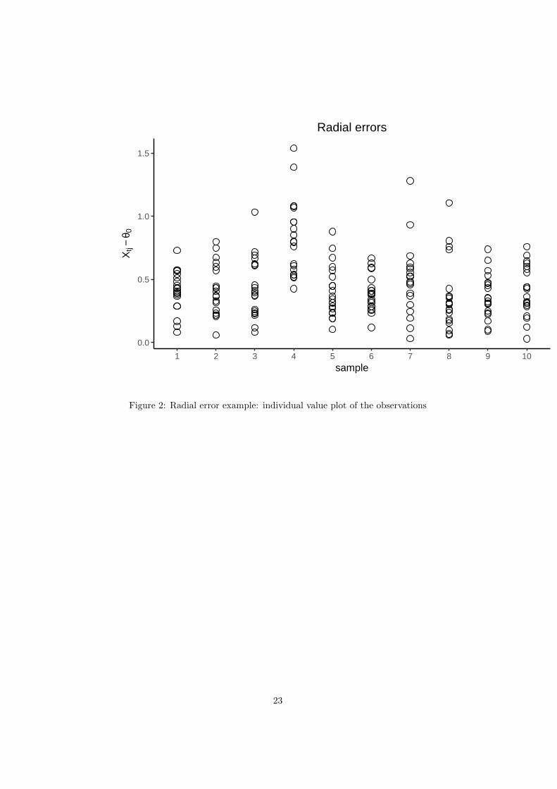
In this Section an illustrative example is provided to show a practical Phase IIimplementation of the design and operation of our proposed chart. This examplewas originally discussed by Celano et al. 32 in which the quality characteristic tobe monitored is the radial error, defined as “a quality characteristic frequentlymonitored in hole drilling processes of mechanical parts and assembly processesof printed circuit boards”. At each sampling point t, a subgroup of size n = 20is collected in order to detect a shift in the median of the quality of interest suchthat p0 = 0.5 shifts to p1 = 0.7. As shown in Table 6, the optimal parametersto be used are λ = 0.34 and K = 2.785. In addition, as shown in Celanoet al. 32 the in-control value of the median for the radial error is θ0 = 0.338.In Table 7 the values of the simulated radial errors Xt,j for t ∈ {1, 2 . . . , 10}and j ∈ {1, 2 . . . , 20} are provided and the values of SRt, SR∗t , and Z∗t arealso reported. In Figure 2 the differences Xt,j − θ0 for t ∈ {1, 2 . . . , 10} areplotted, where at each sampling point, t, more than one values correspond toties between the differences of Xt,j and θ0. The values of the charting statisticZ∗t are plotted in Figure 3. It can be seen that at the 4th sampling point (t = 4)an out-of-control signal is given stating that the process median has changed.

5 Conclusions

In this paper we proposed a modified distribution-free EWMA control chartbased on the Wilcoxon signed rank statistic called as the C-WSR EWMA chart.We aimed to present a robust technique which guarantees steady results for itsRun Length properties. Using the “continuousify” method introduced by Wuet al. 26 we determined its RL properties showing that the number of cutpointsdoes not affect the results. Additionally, we tested the efficiency of this methodunder the use of several kernels besides the Gaussian and we saw that no sig-nificant differences exist. It should be noted that our work was mainly focusedon providing an enhanced method for the determination of the chart’s RL prop-erties rather than examining its superiority versus other schemes. It is worthstretching that, its in- and out-of-control performances were derived regardlessthe process underlying distribution for monitoring any percentile of interest.

As a future work many things can be pursued. For instance, the “continuousify”method could be applied in EWMA-type schemes where other nonparametricstatistics are considered such as the Mann-Whitney, and the Ansari-Bradleystatistics. Additionally, it would be interesting to examine the performance ofthe C-WSR EWMA chart in the presence of ties in the population. Finally, itwould be challenging to investigate the use of similar kernel-based techniques indistribution-free EWMA schemes designed for monitoring bivariate processes.

Appendix

Let as denote EN (X) = µ and VN (X) = σ2 as the mean and variance of arandom variable, X, from a Normal distribution. For the computation of themean of SR∗t we have:

11

E(SR∗t ) =

∫ ∞−∞

s× fSR∗t(s|n, p1)ds

=

∫ ∞−∞

s×∑ψ∈Ψ

fSR+t

(ψ + n(n+1)

2

2|n, p1

)× fN(s|ψ, σ)ds

=∑ψ∈Ψ

[fSR+

t

(ψ + n(n+1)

2

2|n, p1

)×∫ ∞−∞

s× fN(s|ψ, σ)ds

]

=∑ψ∈Ψ

[fSR+

t

(ψ + n(n+1)

2

2|n, p1

)× EN (s)

]

=∑ψ∈Ψ

[fSR+

t

(ψ + n(n+1)

2

2|n, p1

)× ψ

]= E(SRt)

Similarly, using the fact that E(SR∗t ) = E(SRt) the variance of SR∗t is computedas:

V(SR∗t ) = E (SR∗t )2 −

(E(SR∗t )

)2=

∫ ∞−∞

s2 × fSR∗t(s|n, p1)ds−

(E(SR∗t )

)2=

∫ ∞−∞

s2 ×∑ψ∈Ψ

[fSR+

t

(ψ + n(n+1)

2

2|n, p1

)× fN(s|ψ, σ)

]ds−

(E(SRt)

)2=∑ψ∈Ψ

[fSR+

t

(ψ + n(n+1)

2

2|n, p1

)×∫ ∞−∞

s2 × fN(s|ψ, σ)ds

]−(E(SRt)

)2=∑ψ∈Ψ

[fSR+

t

(ψ + n(n+1)

2

2|n, p1

)× EN (s2)

]−(E(SRt)

)2=∑ψ∈Ψ

[fSR+

t

(ψ + n(n+1)

2

2|n, p1

)×(VN (s) + (EN (s))2

)]−(E(SRt)

)2=∑ψ∈Ψ

[fSR+

t

(ψ + n(n+1)

2

2|n, p1

)×(σ2 + ψ2

)]−(E(SRt)

)2= σ2 ×

∑ψ∈Ψ

fSR+t

(ψ + n(n+1)

2

2|n, p1

)+∑ψ∈Ψ

ψ2 × fSR+t

(ψ + n(n+1)

2

2|n, p1

)−(E(SRt)

)2= σ2 + E (SRt)

2 −(E(SRt)

)2= σ2 + V(SRt)

12

References

[1] W.A. Shewhart. Statistical Method from the Viewpoint of quality control,Graduate School of Agriculture. Washington, DC, 1939.

[2] SW Roberts. Control chart tests based on geometric moving averages.Technometrics, 1:239–250, 1959.

[3] E.S. Page. Continuous Inspection Schemes. Biometrika, 41(1/2):100–115,1954.

[4] S. Chakraborti, P. Van der Laan, and S.T. Bakir. Nonparametric ControlCharts: an Overview and Some Results. Journal of Quality Technology, 33(3):304–315, 2001.

[5] Peihua Qiu. Some perspectives on nonparametric statistical process control.Journal of Quality Technology, 50(1):49–65, 2018.

[6] S. Chakraborti and M.A. Graham. Nonparametric (Distribution-Free)Control Charts: An Updated Overview and Some Results. Quality En-gineering, 31(4):523–544, 2019.

[7] R.W. Amin and A.J. Searcy. A Nonparametric Exponentially WeightedMoving Average Control Scheme. Communications in Statistics-Simulationand Computation, 20(4):1049–1072, 1991.

[8] M.A. Graham, S. Chakraborti, and S.W. Human. A NonparametricEWMA Sign Chart for Location Based on Individual Measurements. Qual-ity Engineering, 23(3):227–241, 2011.

[9] S.-F. Yang, J.-S. Lin, and S.W. Cheng. A New Nonparametric EWMASign Control Chart. Expert Systems with Applications, 38(5):6239–6243,2011.

[10] M. Aslam, M. Azam, and C.H. Jun. A New Exponentially Weighted Mov-ing Average Sign Chart using Repetitive Sampling. Journal of ProcessControl, 24(7):1149–1153, 2014.

[11] M. Riaz. A Sensitive Non-Parametric EWMA Control Chart. Journal ofthe Chinese Institute of Engineers, 38(2):208–219, 2015.

[12] S.L. Lu. An Extended Nonparametric Exponentially Weighted MovingAverage Sign Control Chart. Quality and Reliability Engineering Interna-tional, 31(1):3–13, 2015.

[13] A. Haq. A New Nonparametric Synthetic EWMA Control Chart for Mon-itoring Process Mean. Communications in Statistics-Simulation and Com-putation, 48(6):1665–1676, 2019.

[14] S.Y. Li, L.C. Tang, and S.H. Ng. Nonparametric CUSUM and EWMAControl Charts for Detecting Mean Shifts. Journal of Quality Technology,42(2):209–226, 2010.

[15] M.A. Graham, S. Chakraborti, and S.W. Human. A Nonparametric Expo-nentially Weighted Moving Average Signed-Rank Chart for Monitoring Lo-cation. Computational Statistics & Data Analysis, 55(8):2490–2503, 2011.

13

[16] N. Chakraborty, S. Chakraborti, S.W. Human, and N. Balakrishnan. AGenerally Weighted Moving Average Signed-Sank Control Chart. Qualityand Reliability Engineering International, 32(8):2835–2845, 2016.

[17] H.Z. Abid, M.and Nazir, M. Riaz, and Z. Lin. An Efficient NonparametricEWMA Wilcoxon Signed-Rank Chart for Monitoring Location. Qualityand Reliability Engineering International, 33(3):669–685, 2017.

[18] Muhammad Ali Raza, Tahir Nawaz, Muhammad Aslam, Sajjad HaiderBhatti, and Rehan Ahmed Khan Sherwani. A New Nonparametric Dou-ble Exponentially Weighted Moving Average Control Chart. Quality andReliability Engineering International, 36(1):68–87, 2020.

[19] Vasileios Alevizakos, Christos Koukouvinos, and Kashinath Chatterjee. ANonparametric Double Generally Weighted Moving Average Signed-RankControl Chart for Monitoring Process Location. Quality and ReliabilityEngineering International, 2020.

[20] K Mabude, JC Malela-Majika, P Castagliola, and SC Shongwe. Gener-ally Weighted Moving Average Monitoring Schemes–Overview and Per-spectives.

[21] D. Brook and D.A. Evans. An Approach to the Probability Distribution ofCUSUM Run Length. Biometrika, 59(3):539–549, 1972.

[22] C.H. Weiß. EWMA Monitoring of Correlated Processes of Poisson Counts.Quality Technology & Quantitative Management, 6(2):137–153, 2009.

[23] P. Castagliola, K.P. Tran, G. Celano, A.C. Rakitzis, and P.E. Maravelakis.An EWMA-Type Sign Chart With Exact Run Length Properties. Journalof Quality Technology, 51(1):51–63, 2019.

[24] A.C. Rakitzis, P. Castagliola, and P.E. Maravelakis. A New Memory-typeMonitoring Technique for Count Data. Computers & Industrial Engineer-ing, 85:235–247, 2015.

[25] A. Tang, J. Sun, X. Hu, and P. Castagliola. A New Nonparametric AdaptiveEWMA Control Chart with Exact Run Length Properties. Computers &Industrial Engineering, 130:404–419, 2019.

[26] S. Wu, P. Castagliola, and G. Celano. A Distribution-free EWMA ControlChart for Monitoring Time-Between-Events-and-Amplitude Data. Journalof Applied Statistics, pages 1–21, 2020.

[27] Jean Dickinson Gibbons and Subhabrata Chakraborti. Nonparametric Sta-tistical Inference: Revised and Expanded. CRC press, 2014.

[28] R.L. McCornack. Extended Tables of the Wilcoxon Matched Pair SignedRank Statistic. Journal of the American Statistical Association, 60(311):864–871, 1965.

[29] B.M. Bennett. On the Non-Null Distribution of Wilcoxon’s Signed RankTest. Metrika, 19(1):36–38, 1972.

14

[30] M.F. Neuts. Matrix-Geometric Solutions in Stochastic Models: an Algo-rithmic Approach. Dover Publications Inc, New York, 1981.

[31] G. Latouche and V. Ramaswami. Introduction to Matrix Analytic Methodsin Stochastic Modeling. ASA-SIAM, Philadelphia, 1999.

[32] G. Celano, P. Castagliola, S. Chakraborti, and G. Nenes. On the Imple-mentation of the Shewhart Sign Control Chart for Low-volume Production.International Journal of Production Research, 54(19):5886–5900, 2016.

Table 1: Implementation Example Data

t SRt SR∗t Z∗t

1 -11 -10.6823 02 21 20.9128 4.18263 27 26.5635 8.65874 -9 -9.2340 5.08025 1 0.9568 4.25556 -21 -21.0686 07 3 2.9014 0.58038 17 17.1334 3.89099 11 10.7754 5.267810 5 5.2996 5.2742

15

Table 2: Comparison of out-of-control ARL values for the WSR EWMA (with-out “continuousify”) and C-WSR EWMA (with “continuousify” and σ = 0.2)chart when λ = 0.2 and K = 2.7

(n=

7,p

1=

0.53

)(n

=8,p

1=

0.6)

(n=

13,p

1=

0.53

)(n

=20,p

1=

0.5)

mW

SR

EW

MA

C-W

SR

EW

MA

WS

RE

WM

AC

-WS

RE

WM

AW

SR

EW

MA

C-W

SR

EW

MA

WS

RE

WM

AC

-WS

RE

WM

A

100

149.

615

0.4

27.6

28.4

108.

9109.

1351

.0328

.211

017

8.5

150.4

27.4

28.4

109.

2109.

2327

.7328

.012

011

7.8

150.4

26.8

28.4

109.

5109.

2310

.6329

.213

017

8.4

150.4

26.5

28.4

109.

0109.

1327

.8328

.014

029

1.8

150.4

30.6

28.4

109.

2109.

2328

.1328

.015

015

3.7

150.4

28.3

28.4

109.

1109.

2341

.3328

.016

027

5.3

150.4

29.3

28.4

109.

2109.

2328

.0328

.017

011

5.5

150.4

27.2

28.4

109.

0109.

2307

.3328

.018

015

8.8

150.4

26.3

28.4

108.

9109.

2363

.7328

.019

035

4.4

150.4

29.0

28.4

109.

3109.

2337

.4328

.020

014

9.1

150.4

26.0

28.4

109.

2109.

2357

.2328

.021

022

5.0

150.4

29.8

28.4

109.

1109.

2315

.2328

.022

012

0.9

150.4

29.5

28.4

109.

2109.

2328

.6328

.023

013

6.3

150.4

30.5

28.4

109.

2109.

2380

.8328

.024

011

2.9

150.4

29.7

28.4

109.

2109.

2364

.9328

.225

016

2.3

150.4

29.0

28.4

109.

1109.

2303

.6328

.026

028

1.8

150.4

28.2

28.4

109.

2109.

2355

.3328

.027

018

3.6

150.4

27.3

28.4

109.

2109.

2349

.3328

.028

018

3.4

150.4

29.9

28.4

109.

2109.

2327

.5328

.029

017

8.1

150.4

26.4

28.4

109.

2109.

2349

.4327

.830

011

3.0

150.4

28.0

28.4

109.

2109.

2366

.8328

.031

011

7.7

150.4

27.6

28.4

109.

1109.

2300

.0328

.032

012

4.1

150.4

27.3

28.4

109.

2109.

2325

.4328

.033

012

8.4

150.4

28.2

28.4

109.

2109.

2354

.7328

.034

025

3.1

150.4

30.0

28.4

109.

0109.

2321

.2328

.035

014

6.5

150.4

27.0

28.4

109.

1109.

2357

.6328

.036

012

4.4

150.4

27.5

28.4

109.

5109.

2357

.0328

.137

012

8.7

150.4

26.6

28.4

109.

2109.

2297

.2328

.038

020

9.7

150.4

26.8

28.4

109.

3109.

2306

.1328

.039

011

2.0

150.4

26.5

28.4

109.

2109.

2328

.1328

.040

011

4.2

150.4

27.0

28.4

109.

2109.

2293

.0328

.0

sim

150.4

28.3

109.0

326.7

16

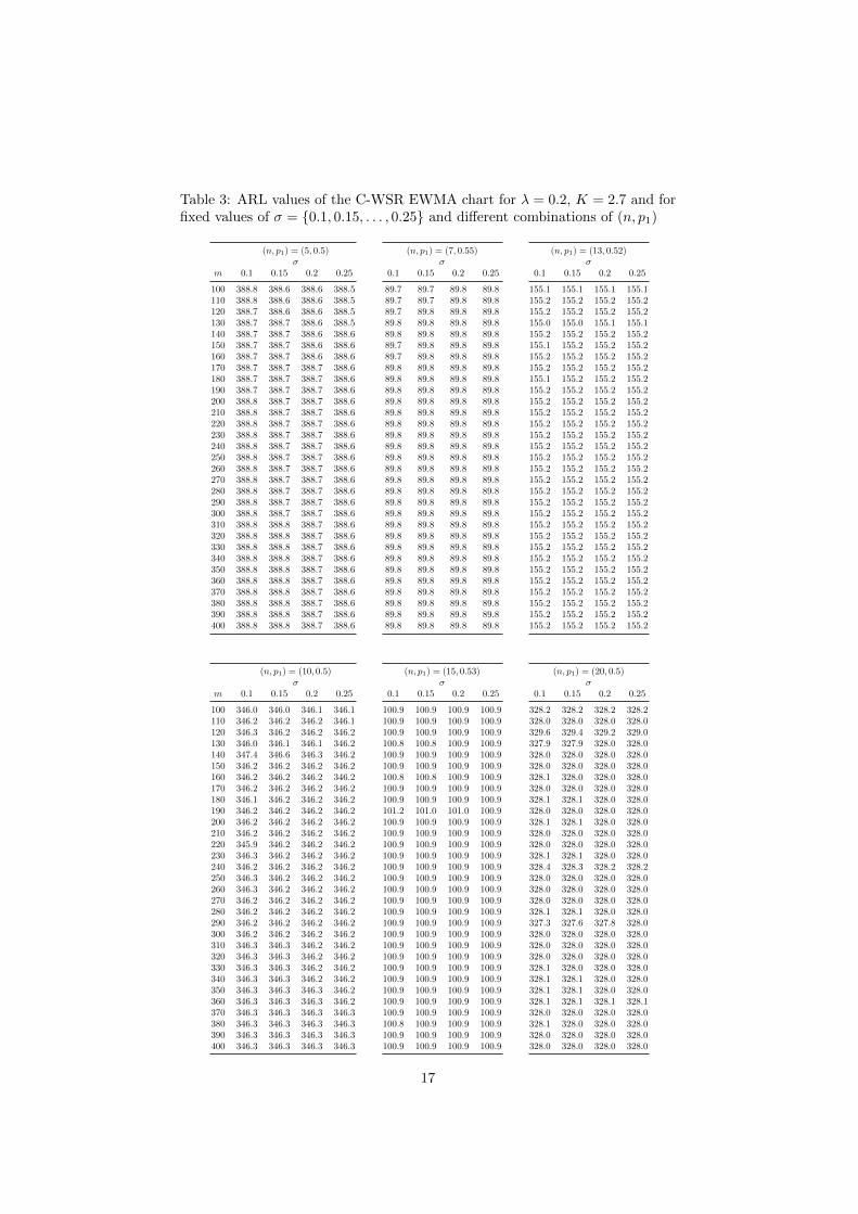
Table 3: ARL values of the C-WSR EWMA chart for λ = 0.2, K = 2.7 and forfixed values of σ = {0.1, 0.15, . . . , 0.25} and different combinations of (n, p1)

(n, p1) = (5, 0.5) (n, p1) = (7, 0.55) (n, p1) = (13, 0.52)σ σ σ

m 0.1 0.15 0.2 0.25 0.1 0.15 0.2 0.25 0.1 0.15 0.2 0.25

100 388.8 388.6 388.6 388.5 89.7 89.7 89.8 89.8 155.1 155.1 155.1 155.1110 388.8 388.6 388.6 388.5 89.7 89.7 89.8 89.8 155.2 155.2 155.2 155.2120 388.7 388.6 388.6 388.5 89.7 89.8 89.8 89.8 155.2 155.2 155.2 155.2130 388.7 388.7 388.6 388.5 89.8 89.8 89.8 89.8 155.0 155.0 155.1 155.1140 388.7 388.7 388.6 388.6 89.8 89.8 89.8 89.8 155.2 155.2 155.2 155.2150 388.7 388.7 388.6 388.6 89.7 89.8 89.8 89.8 155.1 155.2 155.2 155.2160 388.7 388.7 388.6 388.6 89.7 89.8 89.8 89.8 155.2 155.2 155.2 155.2170 388.7 388.7 388.7 388.6 89.8 89.8 89.8 89.8 155.2 155.2 155.2 155.2180 388.7 388.7 388.7 388.6 89.8 89.8 89.8 89.8 155.1 155.2 155.2 155.2190 388.7 388.7 388.7 388.6 89.8 89.8 89.8 89.8 155.2 155.2 155.2 155.2200 388.8 388.7 388.7 388.6 89.8 89.8 89.8 89.8 155.2 155.2 155.2 155.2210 388.8 388.7 388.7 388.6 89.8 89.8 89.8 89.8 155.2 155.2 155.2 155.2220 388.8 388.7 388.7 388.6 89.8 89.8 89.8 89.8 155.2 155.2 155.2 155.2230 388.8 388.7 388.7 388.6 89.8 89.8 89.8 89.8 155.2 155.2 155.2 155.2240 388.8 388.7 388.7 388.6 89.8 89.8 89.8 89.8 155.2 155.2 155.2 155.2250 388.8 388.7 388.7 388.6 89.8 89.8 89.8 89.8 155.2 155.2 155.2 155.2260 388.8 388.7 388.7 388.6 89.8 89.8 89.8 89.8 155.2 155.2 155.2 155.2270 388.8 388.7 388.7 388.6 89.8 89.8 89.8 89.8 155.2 155.2 155.2 155.2280 388.8 388.7 388.7 388.6 89.8 89.8 89.8 89.8 155.2 155.2 155.2 155.2290 388.8 388.7 388.7 388.6 89.8 89.8 89.8 89.8 155.2 155.2 155.2 155.2300 388.8 388.7 388.7 388.6 89.8 89.8 89.8 89.8 155.2 155.2 155.2 155.2310 388.8 388.8 388.7 388.6 89.8 89.8 89.8 89.8 155.2 155.2 155.2 155.2320 388.8 388.8 388.7 388.6 89.8 89.8 89.8 89.8 155.2 155.2 155.2 155.2330 388.8 388.8 388.7 388.6 89.8 89.8 89.8 89.8 155.2 155.2 155.2 155.2340 388.8 388.8 388.7 388.6 89.8 89.8 89.8 89.8 155.2 155.2 155.2 155.2350 388.8 388.8 388.7 388.6 89.8 89.8 89.8 89.8 155.2 155.2 155.2 155.2360 388.8 388.8 388.7 388.6 89.8 89.8 89.8 89.8 155.2 155.2 155.2 155.2370 388.8 388.8 388.7 388.6 89.8 89.8 89.8 89.8 155.2 155.2 155.2 155.2380 388.8 388.8 388.7 388.6 89.8 89.8 89.8 89.8 155.2 155.2 155.2 155.2390 388.8 388.8 388.7 388.6 89.8 89.8 89.8 89.8 155.2 155.2 155.2 155.2400 388.8 388.8 388.7 388.6 89.8 89.8 89.8 89.8 155.2 155.2 155.2 155.2

(n, p1) = (10, 0.5) (n, p1) = (15, 0.53) (n, p1) = (20, 0.5)σ σ σ

m 0.1 0.15 0.2 0.25 0.1 0.15 0.2 0.25 0.1 0.15 0.2 0.25

100 346.0 346.0 346.1 346.1 100.9 100.9 100.9 100.9 328.2 328.2 328.2 328.2110 346.2 346.2 346.2 346.1 100.9 100.9 100.9 100.9 328.0 328.0 328.0 328.0120 346.3 346.2 346.2 346.2 100.9 100.9 100.9 100.9 329.6 329.4 329.2 329.0130 346.0 346.1 346.1 346.2 100.8 100.8 100.9 100.9 327.9 327.9 328.0 328.0140 347.4 346.6 346.3 346.2 100.9 100.9 100.9 100.9 328.0 328.0 328.0 328.0150 346.2 346.2 346.2 346.2 100.9 100.9 100.9 100.9 328.0 328.0 328.0 328.0160 346.2 346.2 346.2 346.2 100.8 100.8 100.9 100.9 328.1 328.0 328.0 328.0170 346.2 346.2 346.2 346.2 100.9 100.9 100.9 100.9 328.0 328.0 328.0 328.0180 346.1 346.2 346.2 346.2 100.9 100.9 100.9 100.9 328.1 328.1 328.0 328.0190 346.2 346.2 346.2 346.2 101.2 101.0 101.0 100.9 328.0 328.0 328.0 328.0200 346.2 346.2 346.2 346.2 100.9 100.9 100.9 100.9 328.1 328.1 328.0 328.0210 346.2 346.2 346.2 346.2 100.9 100.9 100.9 100.9 328.0 328.0 328.0 328.0220 345.9 346.2 346.2 346.2 100.9 100.9 100.9 100.9 328.0 328.0 328.0 328.0230 346.3 346.2 346.2 346.2 100.9 100.9 100.9 100.9 328.1 328.1 328.0 328.0240 346.2 346.2 346.2 346.2 100.9 100.9 100.9 100.9 328.4 328.3 328.2 328.2250 346.3 346.2 346.2 346.2 100.9 100.9 100.9 100.9 328.0 328.0 328.0 328.0260 346.3 346.2 346.2 346.2 100.9 100.9 100.9 100.9 328.0 328.0 328.0 328.0270 346.2 346.2 346.2 346.2 100.9 100.9 100.9 100.9 328.0 328.0 328.0 328.0280 346.2 346.2 346.2 346.2 100.9 100.9 100.9 100.9 328.1 328.1 328.0 328.0290 346.2 346.2 346.2 346.2 100.9 100.9 100.9 100.9 327.3 327.6 327.8 328.0300 346.2 346.2 346.2 346.2 100.9 100.9 100.9 100.9 328.0 328.0 328.0 328.0310 346.3 346.3 346.2 346.2 100.9 100.9 100.9 100.9 328.0 328.0 328.0 328.0320 346.3 346.3 346.2 346.2 100.9 100.9 100.9 100.9 328.0 328.0 328.0 328.0330 346.3 346.3 346.2 346.2 100.9 100.9 100.9 100.9 328.1 328.0 328.0 328.0340 346.3 346.3 346.2 346.2 100.9 100.9 100.9 100.9 328.1 328.1 328.0 328.0350 346.3 346.3 346.3 346.2 100.9 100.9 100.9 100.9 328.1 328.1 328.0 328.0360 346.3 346.3 346.3 346.2 100.9 100.9 100.9 100.9 328.1 328.1 328.1 328.1370 346.3 346.3 346.3 346.3 100.9 100.9 100.9 100.9 328.0 328.0 328.0 328.0380 346.3 346.3 346.3 346.3 100.8 100.9 100.9 100.9 328.1 328.0 328.0 328.0390 346.3 346.3 346.3 346.3 100.9 100.9 100.9 100.9 328.0 328.0 328.0 328.0400 346.3 346.3 346.3 346.3 100.9 100.9 100.9 100.9 328.0 328.0 328.0 328.0

17

Table 4: Some standardized continuous kernels

Kernel Domain K(x)

Parabolic [−√

5,√

5] 34√

5

(1− 1

5x2)

Biweight [−√

7,√

7] 1516√

7(1− x2

7 )2

Triweight [−3, 3] 3596

(1− x6

36 − 3x2

9 + 3x4

34

)Cosine

[− 1√

1− 8π2

, 1√1− 8

π2

] √π2

16 −12 cos

(√π2x2

4 − 2x2

)Normal (−∞,∞) e−x

2/2√

2π

18

Table 5: ARL values of the C-WSR EWMA chart for parameters λ = 0.2,K = 2.7, for σ = 0.2, n ∈ {7, 13, 15, 18, 20, 25} and for the kernels listed inTable 4

n=

7n

=13

n=

15

mP

arab

olic

Biw

eight

Cos

ine

Tri

wei

ght

Nor

mal

Par

abolic

Biw

eight

Cosi

ne

Tri

wei

ght

Nor

mal

Para

boli

cB

iwei

ght

Cos

ine

Tri

wei

ght

Nor

mal

100

363.

636

3.6

363.6

363.

636

3.6

337.

433

7.4

337

.433

7.4

337.3

333.

7333

.733

3.7

333.

733

3.7

110

363.

636

3.6

363.6

363.

636

3.6

337.

433

7.4

337

.433

7.4

337.4

333.

8333

.833

3.8

333.

833

3.8

120

363.

636

3.6

363.6

363.

636

3.6

337.

533

7.5

337

.533

7.5

337.5

333.

8333

.833

3.8

333.

833

3.8

130

363.

636

3.6

363.6

363.

636

3.6

337.

233

7.2

337

.233

7.2

337.1

333.

7333

.733

3.7

333.

733

3.7

140

363.

736

3.7

363.7

363.

736

3.6

337.

533

7.4

337

.533

7.4

337.4

333.

8333

.833

3.8

333.

833

3.8

150

363.

636

3.7

363.6

363.

736

3.7

337.

533

7.5

337

.533

7.5

337.5

333.

8333

.833

3.8

333.

833

3.8

160

363.

636

3.7

363.6

363.

736

3.7

337.

533

7.5

337

.533

7.5

337.5

333.

7333

.733

3.7

333.

733

3.7

170

363.

736

3.7

363.6

363.

736

3.7

337.

533

7.5

337

.533

7.5

337.5

333.

8333

.833

3.8

333.

833

3.8

180

363.

736

3.7

363.7

363.

736

3.7

337.

533

7.5

337

.533

7.5

337.5

333.

8333

.833

3.8

333.

833

3.8

190

363.

736

3.7

363.7

363.

736

3.7

337.

533

7.5

337

.533

7.5

337.5

333.

9333

.933

3.9

334.

033

4.1

200

363.

736

3.7

363.7

363.

736

3.7

337.

533

7.5

337

.533

7.5

337.5

333.

8333

.833

3.8

333.

833

3.8

210

363.

736

3.7

363.7

363.

736

3.7

337.

533

7.5

337

.533

7.5

337.5

333.

8333

.833

3.8

333.

833

3.8

220

363.

736

3.7

363.7

363.

736

3.7

337.

533

7.5

337

.533

7.5

337.5

333.

8333

.833

3.8

333.

833

3.8

230

363.

736

3.7

363.7

363.

736

3.7

337.

533

7.5

337

.533

7.5

337.5

333.

8333

.833

3.8

333.

833

3.8

240

363.

736

3.7

363.7

363.

736

3.7

337.

533

7.5

337

.533

7.5

337.5

333.

8333

.833

3.8

333.

833

3.8

250

363.

736

3.7

363.7

363.

736

3.7

337.

533

7.5

337

.533

7.5

337.5

333.

8333

.833

3.8

333.

833

3.8

260

363.

736

3.7

363.7

363.

736

3.7

337.

533

7.5

337

.533

7.5

337.5

333.

8333

.833

3.8

333.

833

3.8

270

363.

736

3.7

363.7

363.

736

3.7

337.

533

7.5

337

.533

7.5

337.5

333.

8333

.833

3.8

333.

833

3.8

280

363.

736

3.7

363.7

363.

736

3.7

337.

533

7.5

337

.533

7.5

337.5

333.

8333

.833

3.8

333.

833

3.8

290

363.

736

3.7

363.7

363.

736

3.7

337.

533

7.5

337

.533

7.5

337.5

333.

8333

.833

3.8

333.

833

3.8

300

363.

736

3.7

363.7

363.

736

3.7

337.

533

7.5

337

.533

7.5

337.5

333.

8333

.833

3.8

333.

833

3.8

n=

18n

=20

n=

25

mP

arab

olic

Biw

eight

Cos

ine

Tri

wei

ght

Nor

mal

Par

abolic

Biw

eight

Cosi

ne

Tri

wei

ght

Nor

mal

Para

boli

cB

iwei

ght

Cos

ine

Tri

wei

ght

Nor

mal

100

329.

732

9.7

329.7

329.

732

9.7

328.

232

8.2

328

.232

8.2

328.2

324.

6324

.632

4.6

324.

632

4.6

110

329.

732

9.8

329.8

329.

832

9.9

328.

032

8.0

328

.032

8.0

328.0

324.

6324

.632

4.6

324.

632

4.6

120

329.

832

9.8

329.8

329.

832

9.8

329.

132

9.1

329

.132

9.1

329.2

324.

6324

.632

4.6

324.

632

4.6

130

329.

832

9.8

329.8

329.

832

9.9

328.

032

8.0

328

.032

8.0

327.9

324.

5324

.532

4.5

324.

532

4.5

140

329.

932

9.9

329.9

329.

932

9.9

328.

032

8.0

328

.032

8.0

328.0

324.

8324

.832

4.8

324.

832

4.8

150

329.

932

9.9

329.9

329.

932

9.9

328.

032

8.0

328

.032

8.0

328.0

324.

7324

.732

4.7

324.

732

4.7

160

329.

932

9.9

329.9

329.

932

9.9

328.

032

8.0

328

.032

8.0

328.0

324.

7324

.732

4.7

324.

732

4.7

170

329.

832

9.8

329.8

329.

832

9.8

328.

032

8.0

328

.032

8.0

328.0

324.

8324

.832

4.8

324.

832

4.8

180

329.

932

9.9

329.9

329.

932

9.9

328.

032

8.0

328

.032

8.0

328.0

324.

7324

.732

4.7

324.

732

4.7

190

329.

932

9.9

329.9

329.

932

9.9

328.

032

8.0

328

.032

8.0

328.0

324.

7324

.732

4.7

324.

732

4.7

200

329.

932

9.9

329.9

329.

932

9.9

328.

032

8.0

328

.032

8.0

328.0

324.

7324

.832

4.8

324.

832

4.8

210

329.

832

9.8

329.8

329.

832

9.8

328.

032

8.0

328

.032

8.0

328.0

324.

7324

.732

4.7

324.

732

4.7

220

329.

932

9.9

329.9

329.

932

9.9

328.

032

8.0

328

.032

8.0

328.0

324.

7324

.732

4.7

324.

732

4.7

230

329.

932

9.9

329.9

329.

932

9.9

328.

032

8.0

328

.032

8.0

328.0

324.

7324

.732

4.7

324.

732

4.7

240

329.

932

9.9

329.9

329.

932

9.9

328.

232

8.2

328

.232

8.2

328.2

324.

7324

.732

4.7

324.

732

4.7

250

329.

932

9.8

329.9

329.

832

9.8

328.

032

8.0

328

.032

8.0

328.0

324.

7324

.732

4.7

324.

732

4.7

260

329.

932

9.9

329.9

329.

932

9.9

328.

032

8.0

328

.032

8.0

328.0

324.

7324

.732

4.7

324.

732

4.7

270

329.

932

9.9

329.9

329.

932

9.9

328.

032

8.0

328

.032

8.0

328.0

324.

8324

.832

4.8

324.

832

4.8

280

329.

932

9.9

329.9

329.

932

9.9

328.

032

8.0

328

.032

8.0

328.0

324.

7324

.732

4.7

324.

732

4.7

290

329.

832

9.9

329.9

329.

932

9.9

328.

032

7.9

328

.032

7.9

327.8

324.

7324

.732

4.7

324.

732

4.7

300

329.

932

9.9

329.9

329.

932

9.9

328.

032

8.0

328

.032

8.0

328.0

324.

8324

.832

4.8

324.

832

4.8

19

Table 6: Optimal combinations of (λ∗,K∗) for the C-WSR EWMA chart alongwith the corresponding ARL1 values

p1

n0.

550.

600.

65

0.70

0.75

0.80

0.85

0.9

00.9

5

5(0

.015

,1.9

65,7

3.23

)(0

.045

,2.3

89,3

2.01)

(0.0

8,2.5

5,18.

31)

(0.1

35,2

.648

,11.

96)

(0.1

8,2

.679

,8.4

3)(0

.26,

2.68

5,6.

23)

(0.5

,2.5

7,4.

6)(0

.5,2

.57,3

.43)

(0.5

25,2

.549,2

.61)

6(0

.015

,1.9

64,6

6.97

)(0

.05,

2.42

3,28

.62)

(0.0

9,2.

58,

16.2

3)

(0.1

4,2.6

6,10

.55)

(0.2

,2.6

96,7

.43)

(0.3

25,

2.69

3,5

.44)

(0.4

5,2.

646,

4.09)

(0.5

25,2

.598,3

.14)

(0.7

05,2

.463,2

.44)

7(0

.02,

2.08

7,61

.69)

(0.0

55,2

.452

,25.

98)

(0.1

,2.6

06,

14.6

2)

(0.1

55,2

.68,9

.47)

(0.2

5,2

.716

,6.6

4)(0

.29,

2.71

6,4.

91)

(0.4

,2.6

9,3.

74)

(0.5

3,2

.634,2

.91)

(0.6

05,2

.589,2

.34)

8(0

.02,

2.08

6,57

.41)

(0.0

55,2

.453

,23.

87)

(0.1

1,2.6

27,1

3.3

5)(0

.17,

2.6

97,8

.62)

(0.2

6,2

.727

,6.0

3)(0

.35,

2.72

1,4.

45)

(0.4

15,2

.704

,3.4

2)(0

.465,2

.688,2

.72)

(0.9

45,2

.518,2

.04)

9(0

.025

,2.1

76,5

3.81

)(0

.065

,2.5

02,2

2.09)

(0.1

2,2.6

46,1

2.3

)(0

.19,2

.713

,7.9

2)(0

.275

,2.7

37,5

.54)

(0.3

65,

2.73

1,4

.09)

(0.4

05,2

.722

,3.1

6)(0

.855,2

.612,2

.3)

(0.8

6,2

.61,1

.53)

10(0

.025

,2.1

76,5

0.75

)(0

.07,

2.5

23,2

0.6)

(0.1

3,2.

663

,11.

42)

(0.1

95,2

.72,

7.3

5)(0

.275

,2.7

43,

5.14

)(0

.36,

2.74

1,3.

8)(0

.5,2

.708

,2.9

6)(0

.715,2

.66,2

.11)

(0.8

25,2

.646,1

.5)

11(0

.03,

2.24

7,48

.01)

(0.0

75,2

.542

,19.

32)

(0.1

35,2

.671

,10.

68)

(0.2

15,2

.734

,6.8

5)(0

.31,

2.752

,4.7

9)(0

.37,

2.748

,3.5

6)

(0.6

2,2.

695,2

.65)

(0.6

2,2

.695,1

.99)

(0.7

6,2

.668,1

.46)

12(0

.03,

2.24

6,45

.68)

(0.0

75,2

.542

,18.

22)

(0.1

4,2.

679

,10.

04)

(0.2

25,2

.741

,6.4

3)

(0.3

05,2

.757,

4.5

)(0

.395

,2.7

52,

3.35

)(0

.555

,2.7

21,2

.49)

(0.6

45,2

.704,1

.89)

(0.7

8,2

.676,1

.41)

13(0

.03,

2.24

6,43

.56)

(0.0

85,2

.575

,17.

25)

(0.1

5,2.

693

,9.4

8)

(0.2

3,2.

746,

6.0

7)(0

.31,

2.7

62,4

.25)

(0.5

,2.7

41,3

.13)

(0.5

65,2

.73,

2.37

)(0

.705,2

.702,1

.8)

(0.7

85,2

.689,1

.35)

14(0

.03,

2.24

6,41

.68)

(0.0

75,2

.543

,16.

39)

(0.1

6,2.

704

,8.9

8)

(0.2

5,2.

755,

5.7

4)(0

.355

,2.7

67,

4.02

)(0

.46,

2.756

,2.9

7)

(0.6

1,2.

731,2

.25)

(0.7

65,2

.703,1

.7)

(0.9

2,2

.659,1

.28)

15(0

.035

,2.3

03,4

0)(0

.1,2

.615

,15.

63)

(0.1

65,2

.71,8

.55)

(0.2

6,2.

761,

5.46

)(0

.35,2

.771

,3.8

3)(0

.48,

2.76

,2.8

3)(0

.67,

2.73

,2.1

4)(0

.855,2

.692,1

.6)

(0.9

3,2

.664,1

.21)

16(0

.035

,2.3

03,3

8.42

)(0

.11,

2.63

7,14

.92)

(0.1

8,2.

724

,8.1

5)

(0.2

6,2.

763,

5.2

1)(0

.39,

2.7

73,3

.65)

(0.4

95,2

.763

,2.7

)(0

.68,

2.73

6,2.

03)

(0.9

3,2

.68,1

.49)

(0.9

4,2

.679,1

.13)

17(0

.035

,2.3

03,3

7.02

)(0

.1,2

.616

,14.

32)

(0.1

8,2.

725

,7.7

9)

(0.2

75,2

.769

,4.9

8)

(0.3

85,2

.777

,3.4

9)

(0.5

25,2

.765

,2.5

8)(0

.755

,2.7

29,1

.91)

(0.8

85,2

.701,1

.42)

(0.9

45,2

.675,1

.11)

18(0

.04,

2.35

,35.

74)

(0.1

05,2

.627,

13.7

5)(0

.19,

2.734

,7.4

8)

(0.2

75,2

.771

,4.7

8)

(0.3

85,2

.781

,3.3

5)

(0.5

7,2.

764

,2.4

6)

(0.7

3,2.

741,1

.82)

(0.8

35,2

.722,1

.37)

(0.8

35,2

.722,1

.1)

19(0

.035

,2.3

02,3

4.58

)(0

.105

,2.6

28,1

3.24

)(0

.195

,2.7

39,

7.19)

(0.2

9,2.

776,

4.5

9)(0

.405

,2.7

83,

3.22

)(0

.605

,2.7

64,2

.35)

(0.7

3,2.

747,

1.7

5)(0

.875

,2.7

14,1

.32)

(0.8

75,2

.714,1

.08)

20(0

.04,

2.35

,33.

45)

(0.1

15,2

.648,

12.7

6)(0

.2,2

.743

,6.9

2)

(0.3

4,2.

785,

4.4

1)(0

.47,

2.7

82,3

.09)

(0.6

05,2

.769,

2.26

)(0

.805

,2.7

38,1

.67)

(0.9

,2.7

12,1

.27)

(0.9

,2.7

12,1

.06)

20

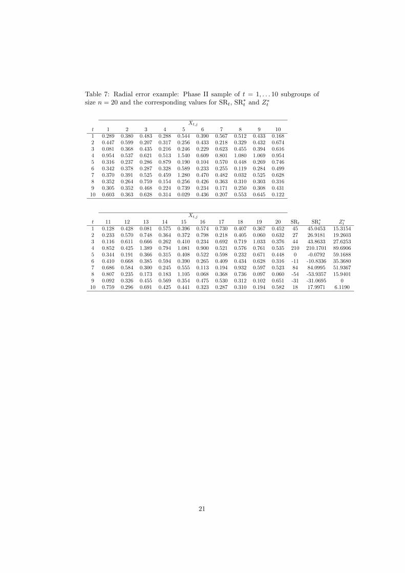
Table 7: Radial error example: Phase II sample of t = 1, . . . 10 subgroups ofsize n = 20 and the corresponding values for SRt, SR∗t and Z∗t

Xt,j

t 1 2 3 4 5 6 7 8 9 101 0.289 0.380 0.483 0.288 0.544 0.390 0.567 0.512 0.433 0.1682 0.447 0.599 0.207 0.317 0.256 0.433 0.218 0.329 0.432 0.6743 0.081 0.368 0.435 0.216 0.246 0.229 0.623 0.455 0.394 0.6164 0.954 0.537 0.621 0.513 1.540 0.609 0.801 1.080 1.069 0.9545 0.316 0.237 0.286 0.879 0.190 0.104 0.570 0.448 0.269 0.7466 0.342 0.378 0.287 0.328 0.589 0.233 0.255 0.119 0.284 0.4997 0.370 0.391 0.525 0.459 1.280 0.470 0.482 0.032 0.525 0.6288 0.352 0.264 0.759 0.154 0.256 0.426 0.363 0.310 0.303 0.3169 0.305 0.352 0.468 0.224 0.739 0.234 0.171 0.250 0.308 0.43110 0.603 0.363 0.628 0.314 0.029 0.436 0.207 0.553 0.645 0.122

Xt,j

t 11 12 13 14 15 16 17 18 19 20 SRt SR∗t Z∗t1 0.128 0.428 0.081 0.575 0.396 0.574 0.730 0.407 0.367 0.452 45 45.0453 15.31542 0.233 0.570 0.748 0.364 0.372 0.798 0.218 0.405 0.060 0.632 27 26.9181 19.26033 0.116 0.611 0.666 0.262 0.410 0.234 0.692 0.719 1.033 0.376 44 43.8633 27.62534 0.852 0.425 1.389 0.794 1.081 0.900 0.521 0.576 0.761 0.535 210 210.1701 89.69065 0.344 0.191 0.366 0.315 0.408 0.522 0.598 0.232 0.671 0.448 0 -0.0792 59.16886 0.410 0.668 0.385 0.594 0.390 0.265 0.409 0.434 0.628 0.316 -11 -10.8336 35.36807 0.686 0.584 0.300 0.245 0.555 0.113 0.194 0.932 0.597 0.523 84 84.0995 51.93678 0.807 0.235 0.173 0.183 1.105 0.068 0.368 0.736 0.097 0.060 -54 -53.9357 15.94019 0.092 0.326 0.455 0.569 0.354 0.475 0.530 0.312 0.102 0.651 -31 -31.0695 010 0.759 0.296 0.691 0.425 0.441 0.323 0.287 0.310 0.194 0.582 18 17.9971 6.1190

21

380

385

390

395

400

405

100 150 200 250 300 350 400 450 500

ARL0

m

n = 5

344

345

346

347

348

349

100 150 200 250 300 350 400 450 500

ARL0

m

n = 10

250

300

350

400

450

500

100 150 200 250 300 350 400 450 500

ARL0

m

n = 15

300

320

340

360

380

100 150 200 250 300 350 400 450 500

ARL0

m

n = 20

Figure 1: ARL0 (plain lines) in function of the number of sub-intervals m ∈{100, 110, . . . , 500} for the upper-sided WSR EWMA chart with parameters(λ = 0.2,K = 2.7) and n ∈ {5, 10, 15, 20} using the standard Markov Chainmethod

22

0.0

0.5

1.0

1.5

1 2 3 4 5 6 7 8 9 10sample

Xtj

−θ 0

Radial errors

Figure 2: Radial error example: individual value plot of the observations

23

UCLUCLUCLUCLUCLUCLUCLUCLUCLUCL

0

25

50

75

1 2 3 4 5 6 7 8 9 10sample

Zt*

C−WSR EWMA chart for Phase II data

Figure 3: Radial error example: the C-WSR EWMA chart for the Phase II datapresented in Table 7

24