An Analysis of the Costs and Benefits to Consumers and Growers

from the Consumption of Recommended Amounts and Types of Fruits and Vegetables for Cancer Prevention

Final report prepared for the California Department of Health Services Cancer Prevention and Nutrition Section

By

Karen M. Jetter

James A. Chalfant Daniel A. Sumner

University of California Agricultural Issues Center

April 2004

Karen M. Jetter is Research Economist with the Agricultural Issues Center, University of California, James A. Chalfant is Professor and Chair, Department of Agricultural and Resource Economics, University of California, Davis, and Daniel A. Sumner is Frank H. Buck, Jr. Chair, Department of Agricultural and Resource Economics, University of California, Davis, and Director, Agricultural Issues Center, University of California. This material was developed for the California Department of Health Services and the California Nutrition Network with funding support from the U.S. Department of Agriculture's Food Stamp Program. This research was also made possible by funds received from the Cancer Research Fund, under grant agreement No. 98-16026 with the Department of Health Services, Cancer Research Program.

1

An Analysis of the Private Costs and Benefits to Consumers and Growers from Eating Recommended Amounts and Types of Fruits and Vegetables for Cancer Prevention EXECUTIVE SUMMARY This study examines the direct economic benefits and costs of Californian consumers adopting four alternative recommended diets: the very minimum 5-a-day recommendation for fruits and vegetables, the 5-a-day commodity sub-group recommendations for a cancer prevention diet, the 7-a-day minimum recommendation for men and active women, and the 7-a-day commodity sub-group recommendations for a cancer prevention diet. The study does not analyze the health consequences of these dietary changes, but focuses on the direct economic consequences from changes in quantities demanded and supplied, and on price responses. This study also examines how changes in fruit and vegetable consumption might affect the use of the land, labor, and water resources used in farm production. Increased consumption of fruits and vegetables has been linked to a decrease in the risk of cancer. In a review of 196 epidemiology studies, scientists determined that the link between fruit and vegetable consumption, and a lower incidence of cancer was probable (WCRF and AIC 1997). In addition, convincing evidence exists linking the consumption of specific fruit and vegetable groups to a reduction in certain types of cancers. Therefore, the cancer risk reduction diet provides recommendations for the composition of fruit and vegetable consumption, as well as the total amount. While the minimum recommendations for fruit and vegetable consumption in general are 2 fruit servings and 3 vegetable servings a day, the USDA minimum recommendations for men and active women are 3 fruit servings and 4 vegetable servings a day (McNamara et al. 1999). The more specific cancer prevention recommendations for the 5-a-day program for fruit are at least 1 serving from the citrus/berry/melon group and at least 1 additional serving of any fruit. For vegetables, the recommendations are at least 1 serving of dark colored vegetables, 1 serving of salad, 0.5 servings of a starchy vegetable, at least 0.5 servings of cruciferous vegetables, and 0.3 servings of tomato. The 7-a-day cancer prevention recommendations add an additional serving of any fruit and an additional 0.7 servings of any vegetable. Despite the known benefits, many people do not eat recommended levels of fruits and vegetables. In some cases the difference between actual and recommended consumption is quite large. Based on data from the California Survey of Dietary Practices, the consumption of dark green and orange vegetables by people in low-income households would need to increase by 307 percent in order to achieve the recommended levels in the 7-a-day cancer prevention program. The shift in quantity demanded toward more fruits and vegetables would be met through increases in supply of produce from several market channels. These include imports from other regions in the U.S. and other countries, and increased production within California. The ability of growers to increase production depends on the availability of resources, such as land, labor and other purchased inputs, at their disposal. An increase in the demand for fruits and vegetables

2

affects prices, which in turn causes feedback effects on quantity demanded and supplied. To calculate the new prices and market supply a market model is developed that links supply and demand in the final market, to the supply and demand in the marketing sector, to grower production, to supply and demand in agricultural input markets. Percentage Increase in Quantity Demanded Needed to Reach Each Recommended Level 5-a-day 5-a-day cpb 7-a-day 7-a-day cp Income Level a

Low High Low High Low High Low High Citrus-Berry-Melon 8 7 35 32 62 60 92 87 Other Fruit 8 7 -10 -10 62 60 42 42 Starchy Vegetables 75 50 121 92 134 100 157 120 Salad 75 50 147 85 134 100 187 113 Other Vegetable 75 50 -30 -34 134 100 16 15 Tomatoes 75 50 19 6 134 100 39 21 Dark Green and Orange 75 50 250 226 134 100 307 275 Cruciferous 75 50 106 75 134 100 139 101 Potatoes -67 -69 -59 -60 -56 -58 -52 -54 aLow income is less than $15,000 a year. High income is equal to or greater than $15,000 a year. bAs noted in the text, the cp (cancer prevention) diet is more specific than the general fruit and vegetable recommendations. Main Results Even though the shift in quantity demanded by Californians is large in percentage terms, it is small relative to the total market for produce in the U.S., and smaller yet when the potential expansion of supply from imports is considered. Therefore, the implied changes in U.S. market prices are relatively small. This is because Californians only make up 12 percent of the total U.S. market, and when prices rise, there is a decrease in consumption by people in the rest of the U.S. Furthermore, slightly higher prices in the U.S. market attract additional imports. For commodities with a large share of market supply traded internationally, the ability to increase imports or decrease exports are a significant factor in keeping the change in market prices relatively low. Consumers substitute away from the commodities with the greatest increase in prices, and into the commodities with the lowest increase in prices. This affects the projected changes in consumption patterns as people shift into eating better diets. Consumption of some items (grapefruit, bananas, pineapples, plums and prunes) is actually higher than the initial increase in demand for Californians and increases for people in the rest of the U.S., even though prices for those commodities are also higher. While the consumption of some items is higher, with higher prices for all fruits and vegetables, total fruit and vegetable consumption is slightly less than the recommended levels for Californians, and decreases for people living in the rest of the U.S. Net economic gains for California consumers are large, with the benefits coming through the assumed large increase in willingness to pay for the increased quantity demanded for fruits and

3

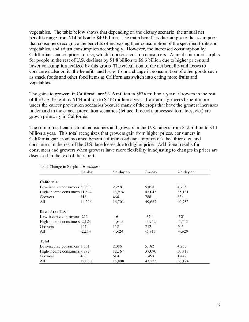
vegetables. The table below shows that depending on the dietary scenario, the annual net benefits range from $14 billion to $49 billion. The main benefit is due simply to the assumption that consumers recognize the benefits of increasing their consumption of the specified fruits and vegetables, and adjust consumption accordingly. However, the increased consumption by Californians causes prices to rise, which imposes a cost on consumers. Annual consumer surplus for people in the rest of U.S. declines by $1.8 billion to $6.6 billion due to higher prices and lower consumption realized by this group. The calculation of the net benefits and losses to consumers also omits the benefits and losses from a change in consumption of other goods such as snack foods and other food items as Californians switch into eating more fruits and vegetables. The gains to growers in California are $316 million to $836 million a year. Growers in the rest of the U.S. benefit by $144 million to $712 million a year. California growers benefit more under the cancer prevention scenarios because many of the crops that have the greatest increases in demand in the cancer prevention scenarios (lettuce, broccoli, processed tomatoes, etc.) are grown primarily in California. The sum of net benefits to all consumers and growers in the U.S. ranges from $12 billion to $44 billion a year. This total recognizes that growers gain from higher prices, consumers in California gain from assumed benefits of increased consumption of a healthier diet, and consumers in the rest of the U.S. face losses due to higher prices. Additional results for consumers and growers when growers have more flexibility in adjusting to changes in prices are discussed in the text of the report.

Total Change in Surplus (in millions) 5-a-day 5-a-day cp 7-a-day 7-a-day cp California Low-income consumers 2,083 2,258 5,858 4,785 High-income consumers 11,894 13,978 43,043 35,131 Growers 316 464 788 836 All 14,296 16,703 49,687 40,753 Rest of the U.S. Low-income consumers -233 -161 -674 -521 High-income consumers -2,123 -1,615 -5,952 -4,713 Growers 144 152 712 606 All -2,214 -1,624 -5,913 -4,629 Total Low-income consumers 1,851 2,096 5,182 4,265 High-income consumers 9,772 12,367 37,090 30,418 Growers 460 619 1,498 1,442 All 12,080 15,080 43,773 36,124

1

INTRODUCTION This study estimates the economic impact on producers and consumers in California, and in the rest of the U.S., from the increase in demand for fruits and vegetables that would have to occur in order for Californians to increase their intake of fruits and vegetables to meet recommendations for a cancer-prevention diet. That impact is measured in changes in the prices of fruits and vegetables, and quantities consumed and produced, that translate easily into net benefit measures. Consumers will pay higher prices for produce, but will of course benefit from healthier diets. This study estimates the effects on to consumers and producers from changes in prices and quantities, but the health-related benefits to consumers and to society from healthier diets are beyond the scope of the study. Increased consumption of fruits and vegetables has been linked to a decrease in the risk of cancer. In a review of 196 epidemiology studies, scientists determined that the link between fruit and vegetable consumption and a lower incidence of cancer was probable (World Cancer Research Fund, 1997). In addition, convincing evidence exists linking the consumption of specific fruit and vegetable groups to reductions in certain types of cancers. For example, eating dark vegetables has been associated with a lower incidence of lung and stomach cancers (World Cancer Research Fund, 1997). Therefore, the cancer risk reduction diet provides recommendations for the composition of fruit and vegetable consumption, as well as the total level. Four scenarios are developed in this study to meet different minimum targeted consumption levels. The first is a general 5-a-day recommendation, the second scenario is for more specific food subgroups within the 5-a-day recommendation, the third is a general 7-a-day recommendation, and the final scenario is for specific food subgroups within the 7-a-day recommendation. Because people with lower incomes eat fewer fruits and vegetables than do people with higher incomes, the change in eating habits and the associated benefits for individuals with lower incomes who move to a diet with more fruits and vegetables may be greater. Consequently, this study distinguishes between people living in lower income households (less than $15,000 a year) and people living in higher income households (more than $15,000 a year). That level of income seems to correspond to a shift in consumption patterns, representing a turning point in the number of servings consumed per day, as income rises. A shift in consumption patterns to the recommended levels would cause the demand for fruits and vegetables to rise significantly, leading to higher prices and increased production, shifting the use of agricultural resources (such as land, labor, and water) into the production of those commodities, and benefiting the entire agricultural sector. Californians consume fruits and vegetables produced throughout the U.S. and in other countries. Thus, it follows that growers in both California and elsewhere benefit from the higher prices and increased production, even though only the demand by Californians is increasing, in the hypothetical scenario that we examine in this report. Previous evaluations of the societal benefits of eating more fruits and vegetables have focused on the reductions in health-care expenditures from a reduction in chronic diseases associated with poor diets, including but not limited to some cancers, diabetes, and heart disease. We take it as a

2

given that healthier diets are desirable, and identify the extent to which agricultural producers benefit from such an outcome. This study represents the first attempt to address the effect on growers who could expect to gain from such an increase. Such a benefit to producers might justify additional public sector investment in promoting healthier diets. Much like the situation with generic advertising of specific commodities, individual producers and even entire industries have limited incentives to invest in promoting healthier diets; there is an underinvestment in promoting such messages by industry, since producers capture only a portion of the benefits to society. Without an increase in consumer incomes, increasing the consumption of fruits and vegetables means decreasing the consumption of at least one other product, whether a less healthy food or any other item. The effect of such a compensating reduction in other purchases, in the absence of any change in total spending by consumers, is beyond the scope of the present study, which considers only fruits and vegetables. Consumer benefits are therefore complicated by uncertainty over both the dollar value of health benefits and the nature of adjustments in other spending. However, we report partial effects on consumer benefits, based on the fruit and vegetable markets.

3

FRUIT AND VEGETABLE RECOMMENDATIONS The USDA’s minimum recommendations for fruit and vegetable general consumption for everyone are 5 servings of fruits and vegetables a day, with 2 servings as fruit and 3 as vegetables (Table 1) (USDA & USDHHS 1996; Young and Kantor 1999). Because some fruits and vegetables are higher in the nutrients and phytochemicals that appear to reduce the risk of cancer, minimum recommendations for specific subgroups were expanded on by the Cancer Prevention and Nutrition Services (CPNS) unit of the California Department of Health Services (CDHS), based on a wide body of literature (see, for example, World Cancer Research Fund, 1997).

Table 1. Fruit and Vegetable Recommendations

5-a-day 5-a-day cancer

prevention 7-a-day 7-a-day cancer

prevention Fruit 2 3 Citrus/berry/melon 1 1 Any fruit 1 2 Vegetable 3 4 Starchy 0.5 0.5 Salad Greens 1 1 Cruciferous 0.5 0.5 Tomato 0.3 0.3 Dark Green and Orange 1 1 Any vegetable 0 0.7

The more specific 5-a-day cancer prevention recommendations for fruit are at least 1 serving from the citrus/berry/melon group and at least 1 additional serving of any fruit. For vegetables, the recommendations are at least 1 serving of dark colored (dark green and deep orange) vegetables, 1 serving of salad, 0.5 servings of a starchy vegetable, at least 0.5 servings of cruciferous vegetables, and 0.3 servings of tomato (Table 1). These recommendations put the consumption of vegetables slightly higher than the 3 a day minimum. While the minimum target for the general population is 5 servings of fruits and vegetables a day, the USDA’s minimum recommendations for most men and active women are 3 fruit servings and 4 vegetable servings a day (McNamara et al. 1999; USDA & USDHH 2000) (Table 1). The more specific cancer-prevention recommendations for fruit are at least 1 serving from the citrus/berry/melon group and at least 2 additional servings of any fruit. For vegetables, the recommendations are at least 1 serving of dark colored (dark green and deep orange) vegetables, 1 serving of salad, 0.5 servings of a starchy vegetable, at least 0.5 servings of cruciferous vegetables, 0.3 servings of tomato, and 0.7 additional servings of any vegetable (CPNS 2002) (Table 1).

4

Despite the known benefits, many people do not eat the recommended levels of fruits and vegetables. National surveys indicate that, on average, adults consume 3.9 servings a day, excluding potatoes consumed as french fries or chips (McNamara et al. 1999; Tippett and Cleveland 1999). In some cases, the gap between average and recommended consumption is quite large. For instance, McNamara et al. (1999) estimate that adult per capita consumption of dark vegetables would need to increase by over 300 percent to meet the 1 serving a day recommendation. People in households that earn less than $15,000 a year average even fewer servings per day than do people in higher income households. Based on the California Survey of Dietary Practices (CSDP), average consumption for low-income consumers is 1.850 servings a day for fruit and 1.874 a day for vegetables (Table 2). Higher income consumers eat slightly more fruits and vegetables. Average consumption by high-income consumers is 1.875 servings of fruit a day and 2.191 servings of vegetables (Table 2). Fruit consumption would need to increase by 62 percent for low-income consumers and by 60 percent for high-income consumers to achieve the 3-a-day recommendation. Vegetable consumption would need to increase by 134 percent for low-income consumers, but just under 100 percent for high-income consumers, for these groups to reach the recommended 4-a-day target.

Table 2. Current Servings per Day Consumed in California by Household Incomea Lower Income Higher Income Difference Food Category (<15,000) (≥15,000) Fruit 1.850 1.870 0.019 Citrus/berry/melon 0.741 0.758 0.017 Other Fruit 1.109 1.112 0.003 Vegetable 1.874 2.191 0.317 Starchy 0.227 0.261 0.035 Salad 0.406 0.540 0.135 Other Vegetable 0.454 0.523 0.069 Tomato 0.251 0.284 0.033 Dark - Non Cruciferous 0.195 0.201 0.006 Dark - Cruciferous 0.091 0.106 0.015 Other Cruciferous 0.089 0.089 0.001 Potato with french fries and chipsb 0.862 0.886 0.024 net french fries and chips 0.162 0.186 0.024 Total 3.725 4.061 0.336 aSource: California Survey of Dietary Practices b(Kantor 1998). Because the CSDP does not include french fries and chips in its dietary estimates, the California data for potato consumption were adjusted to include them these items, for purposes of comparison, using the national average of 0.7 servings of french fries or chips consumed daily in the U.S.

5

Even though overall consumption of fruits and vegetables is higher for people with a higher income, people with lower incomes eat more of certain types of fruits and vegetables. Average consumption of apples, bananas, cabbage, celery, cucumbers, pears, tangerines, watermelon, and all juices but grapefruit juice is greater by people with a household income of less than $15,000 a year. In general, these items have lower retail prices than the other fruits and vegetables. Consumption of high-priced items tends to be lower for the low-income group. For instance, consumption of items such as artichokes and raspberries was zero among the low-income households surveyed. When food categories are broken down into sub-groups, greater variation in the gap in meeting targeted levels for the cancer prevention diet is apparent. Among all food categories, both low- and high-income consumers in California come closest to meeting the recommended target of 0.3 servings for tomatoes. Low-income consumers need to increase consumption of tomatoes by only 0.049 servings, and high-income consumers by just 0.016 servings, to reach recommended targets for a cancer prevention diet (Table 2). At the other end of the spectrum, consumption of dark vegetables would need to increase by 0.714 servings for low-income households, and by 0.693 servings for high-income consumers, to meet recommendations (Table 2). The consumption levels calculated from the California Survey on Dietary Practices (CSDP) are consistent with the results of estimates from national studies for most food categories (Table 3). National consumption of fruits and vegetables has been estimated from the Continuing Survey of Food Intakes by Individuals (CSFII) (McNamara et al 1999; Tippett and Cleveland 1999) and from food supply data (Kantor 1998). The CSDP and the CSFII are 24-hour recall surveys concerning individuals’ consumption of food items. The CSFII is collected throughout the year. The CSDP is conducted bi-annually, in the fall. Food supply data, on the other hand, makes use of production, trade, and waste and spoilage data to estimate per capita consumption of foods.

Table 3. Comparison of Results of Food Consumption Studies Californiaa CSFIIb Food Supplyc

servings per day Citrus, Melon, Berry 0.76 0.74 0.6 Other Fruit 1.11 0.76 0.7 Total Fruit 1.87 1.5 1.3 Dark Vegetable 0.29 0.32 0.3 Starchy Vegetable 1.09d 1.28 d 1.4 d Other Vegetable 1.2 1.53 1.9 Total Vegetable 2.58 3.13 3.6 Total 4.45 4.63 4.9 a Source: California Survey of Dietary Practices, b Source: McNamara et al 1999, c Source: Kantor 1998, d Includes potato chips and french fries (See Table 2).

6

Based on the CSFII, overall consumption of fruits and vegetables is 4.45 servings per day, 0.18 servings less than the U.S. figure of 4.63 servings per day. Californians eat more servings of fruit than the national average, but fewer vegetables. Compared to the servings calculated from the CSFII, Californians average 0.37 more servings of fruit, but 0.55 fewer servings of vegetables than U.S. consumers. Neither the 4.45 servings per day for Californians, nor the 4.63 figure for the U.S. as a whole, is as encouraging when one remembers that these include an average of 0.7 servings per day of potatoes consumed as french fries or chips.

7

THE U.S. HORTICULTURAL INDUSTRY A shift in demand toward more fruits and vegetables would be met through increased production from within California and the rest of the U.S, increased imports from other regions, and a reduction in exports. Agricultural industries stand to benefit significantly, should consumers achieve the recommended levels of fruit and vegetable consumption. The annual farmgate value of U.S. production of fruit and vegetables is $21 billion. California is the largest producer of fruits and vegetables in the country, accounting for 49 percent of the total U.S. value. Tree and vine fruit production in California is 58 percent of the U.S. value, and the value of California’s vegetable and melon production is 39 percent of the U.S. value (USDA 1999a). The volume of fruits and vegetables imported into the U.S. is another $10 billion; because it is a wholesale value, that figure is not directly comparable to the farmgate value of U.S. production above, but it does serve to put the relative importance of U.S. production sources in meeting overall U.S. consumption into further perspective. California accounts for over 99 percent of national production of artichokes, Brussels sprouts, dates, figs, kiwi, clingstone peaches, persimmons, prunes, and raisins. It accounts for at least 50 percent of U.S. production of table grapes, wine grapes, lettuce (head, leaf, and romaine), strawberries, broccoli, plums, celery, carrots, avocados, fresh-market oranges, cauliflower, honeydew, cantaloupes, and processing tomatoes. While it produces less than 50 percent of U.S. production of spinach and asparagus, California is still the largest producer of these items. Among fruits and vegetables of significance in consumption, California produces less than 10% of total U.S. production only for apples, peas, snap beans, potatoes, sweet corn, and orange juice. It does not produce any bananas or pineapple. The ability of California growers to increase production of fruits and vegetables depends on the resources, such as land, water, labor, and other purchased inputs, at their disposal. However, there is not an unlimited supply of land, water, or agricultural labor to the California agricultural sector. O’Brien was the first to address the issue of limited resource availability in meeting the increased demand for fruits and vegetables by U.S. producers (1997). Drawing additional resources into the production of fruit and vegetables will raise the prices of those resources, to the extent that their supply is limited. Other researchers have discussed the potential for increasing the supply of fruits and vegetables from trade, acreage adjustments, and greater use of other purchased inputs (Abbott 1999; Young and Kantor 1999). The U.S. has over 931 million acres devoted to agricultural production. Harvested cropland accounts for 39 million acres, and fruits and vegetables 11 million. California has over 27.7 million acres in agricultural production, with 8.5 million harvested acres (USDA 1999a). While California accounts for only three percent of the harvested cropland in agricultural production in the U.S., it has 22 percent of the land in fruit and vegetable production, and 45 percent of the land in tree and vine fruit production. Because California specializes in the fresh market for fruits and vegetables, and in off-season production, its 49 percent share of the value of fruit and vegetable production is greater than its 22 percent share of land in production. Total farm expenses for the U.S. were $151 billion in 1997 (USDA 1999a). Total farm expenses in California were $17 billion. Labor and other purchased inputs account for over half of

8

production costs in California, but less than half for the rest of the U.S. Within California, labor alone accounts for 28 percent of production costs and is the largest expense category. For the rest of U.S. agriculture, labor is only 10 percent of expenses. California has several large agricultural industries that are labor intensive, including fruits, vegetables, and ornamental nursery plants. Another large cost item for California is irrigation water. Most crops in the U.S. are rainfed. In California, however, almost all crops are grown with purchased water. Surface water is either delivered to farms through a system of aqueducts and canals, or pumped from below ground. Other purchased inputs include seeds, nursery stock, fertilizer, chemicals, and energy. For many commodities, the main source of U.S. supply is through imports. Bananas and pineapples are two commodities whose supply is largely from imports. Other commodities, such as potatoes, and plums and prunes, have a large share of their production exported (Table 4). The larger the share of a commodity that is imported or exported, the easier it may be to meet changes in demand through changes in trade flows. Commodities such as bananas, pineapples, potatoes, plums and prunes, and artichokes have more flexibility in meeting changes in domestic demand through changes in trade than do commodities such as strawberries, peas, processing tomatoes, carrots, onions, snap beans, and cabbage (Table 4). For these commodities, changes in demand would be most likely be met through changes in U.S. production.

9

Table 4. Trade shares for fruits and vegetables.

Crop Share of U.S. net market

supply traded* (%) Net Imports Bananas 99.7 Pineapples 77.1 Artichokes 45.2 Cucumbers 37.4 Eggplant 32.0 Asparagus 31.8 Cantaloupe 31.0 Tomatoes, Fresh 27.7 Avocados 27.7 Honeydews 21.5 Apple 20.0 Peppers, Bell 15.3 Broccoli 11.3 Grapes 6.8 Oranges 5.6 Watermelon 4.8 Peas 2.5 Carrots 1.9 Beans, Snap 1.0 Net Exports Potatoes 83.4 Plums and prunes 62.3 Grapefruit 31.4 Cherries 18.0 Cauliflower 17.0 Celery 11.3 Pears 8.4 Apricots 8.3 Lettuce, All 7.6 Spinach 6.6 Corn, Fresh 6.6 Tangerines and other citrus 6.1 Peaches & Nectarines 5.4 Sweet Potatoes 3.1 Strawberries 2.7 Tomatoes, Processing 2.1 Onions 1.8 Cabbage 0.1 *Net U.S. supply is equal to U.S. production plus imports less exports.

10

MARKET EFFECTS OF INCREASED FRUIT AND VEGETABLE CONSUMPTION If consumers were to choose a cancer prevention diet and eat more fruits and vegetables, the increased consumption could come from three potential sources: increased domestic production, increased imports, and, for fruits and vegetables currently exported, a reduction in exports. When applied to California alone, domestic production would refer to in-state production, and imports then refer to product diverted either from other states or other countries. Under normal circumstances, increased quantities from any of these sources require prices to rise. It will take higher prices for any producers to increase production, either from farming existing acreage more intensively or by bringing more acreage into production. Such acreage is likely to be currently planted for other crops, rather than idle. In addition, imports will increase, and exports decrease, but only if prices increase to lure more product to the market. An increase in demand by Californians could be met without any price increases only if California represented a sufficiently small part of the market, or resources for increasing production were available in larger quantities without any input price increases. Neither assumption is plausible. California’s population is about 12% of U.S. population, so it represents a large share of the market, and the availability of at least some inputs—say, land suitable for vegetable production—is not unlimited. For a demand increase that is exactly equal to the amount needed to get to a new dietary guideline, the resulting price increases, which temper the increases in consumption, mean that the new market equilibrium will be characterized by higher prices and increased consumption, but in quantities that fall short of the dietary recommendation. If the necessary price increases are small, the difference between realized and targeted consumption will be small; however, if the price increases are large, consumers will not come as close to achieving the recommended numbers of servings. Simply modeling an increase in consumption, at current prices, and ignoring these market effects, would produce incorrect estimates of the effects of increasing the demand for fruits and vegetables. In particular, we would underestimate the increased expenditures by consumers, overstate the number of servings of fruits and vegetables consumed, and understate both increased costs of production and benefits to producers. These market effects can be illustrated in a graph (Figure 1). Initially there is an equilibrium point, a, at which the supply curve, S, crosses the original demand curve, D1. The supply curve is upward sloping, because as prices increase, the quantity supplied by producers also increases. The demand curve is downward sloping, representing the fact that as prices increase, consumers demand smaller quantities. At point a, the quantity supplied is exactly equal to the quantity demanded. The original market price is P1 and the original market quantity is Q1. The demand for any product depends on several factors. The initial quantity of fruits and vegetables consumed reflects individual consumers’ choices given their current preferences for fruits and vegetables, their incomes, and current prices. Suppose the quantity axis in figure 1 represents the quantity of all fruits and vegetables (or any particular group for which a specific recommendation is made). The quantity corresponding to the initial market equilibrium at the point labeled a thus might represent the current per capita number of fruit and vegetable servings, labeled as Q1. Suppose also that the difference between Q1 and the recommended number of servings is k. In figure 1, demand is shifted to the right, in parallel, by the amount k,

11

representing the amount by which market demand would shift if consumers all adopted the recommendations of a cancer-prevention diet, namely moving to Q*.

S

D1

D2

Quantity

Price

a

b

k

Q1 Q*Q2

P1

P2

Figure 1. Market Effects When Fruit and Vegetable Consumption Increases The new market equilibrium is point b where demand curve D2 intersects the supply curve S. The new equilibrium market price rises to P2 and the new equilibrium quantity demanded is Q2. The upward-sloping supply curve shows why Q* is not attained—at P2 producers are not willing to supply Q*. The closer to horizontal is the supply curve, the closer to Q* will the actual Q2 turn out to be, and the smaller the increase in price. The steeper is the supply curve, on the other hand, the larger the price increase and the greater the difference between Q2 and Q*. The degree of responsiveness by consumers and producers to changes in prices is called an elasticity. An elasticity is simply a number that represents the percentage change in quantity demanded or supplied that follows from a one percent change in price. For example, if a demand elasticity is –0.5, then a one percent increase in price will cause a one-half percent decrease in quantity demanded. Similarly, if the supply elasticity is 2.0, then a one percent increase in price will cause a two percent increase in quantity supplied. Large supply elasticities from either changes in trade or production are required for an outcome with small price effects and consumption close to targeted levels.

12

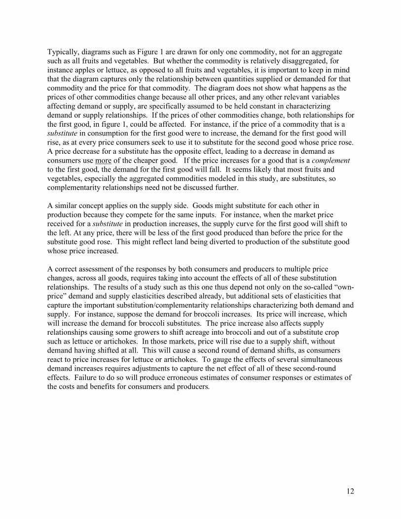
Typically, diagrams such as Figure 1 are drawn for only one commodity, not for an aggregate such as all fruits and vegetables. But whether the commodity is relatively disaggregated, for instance apples or lettuce, as opposed to all fruits and vegetables, it is important to keep in mind that the diagram captures only the relationship between quantities supplied or demanded for that commodity and the price for that commodity. The diagram does not show what happens as the prices of other commodities change because all other prices, and any other relevant variables affecting demand or supply, are specifically assumed to be held constant in characterizing demand or supply relationships. If the prices of other commodities change, both relationships for the first good, in figure 1, could be affected. For instance, if the price of a commodity that is a substitute in consumption for the first good were to increase, the demand for the first good will rise, as at every price consumers seek to use it to substitute for the second good whose price rose. A price decrease for a substitute has the opposite effect, leading to a decrease in demand as consumers use more of the cheaper good. If the price increases for a good that is a complement to the first good, the demand for the first good will fall. It seems likely that most fruits and vegetables, especially the aggregated commodities modeled in this study, are substitutes, so complementarity relationships need not be discussed further. A similar concept applies on the supply side. Goods might substitute for each other in production because they compete for the same inputs. For instance, when the market price received for a substitute in production increases, the supply curve for the first good will shift to the left. At any price, there will be less of the first good produced than before the price for the substitute good rose. This might reflect land being diverted to production of the substitute good whose price increased. A correct assessment of the responses by both consumers and producers to multiple price changes, across all goods, requires taking into account the effects of all of these substitution relationships. The results of a study such as this one thus depend not only on the so-called “own-price” demand and supply elasticities described already, but additional sets of elasticities that capture the important substitution/complementarity relationships characterizing both demand and supply. For instance, suppose the demand for broccoli increases. Its price will increase, which will increase the demand for broccoli substitutes. The price increase also affects supply relationships causing some growers to shift acreage into broccoli and out of a substitute crop such as lettuce or artichokes. In those markets, price will rise due to a supply shift, without demand having shifted at all. This will cause a second round of demand shifts, as consumers react to price increases for lettuce or artichokes. To gauge the effects of several simultaneous demand increases requires adjustments to capture the net effect of all of these second-round effects. Failure to do so will produce erroneous estimates of consumer responses or estimates of the costs and benefits for consumers and producers.

13

MEASURING THE COSTS AND BENEFITS The effects on consumers and growers from an increase in the demand for fruits and vegetables are determined by converting changes in prices and quantities into changes in measures of economic welfare, known as consumer surplus and producer surplus, respectively. These measures of welfare change can be understood most easily by reference to Figure 1. Consider a point on the demand curve that corresponds to a very high market price and a very small quantity demanded. At this point, many consumers would have shifted their consumption to substitute goods, responding to the high price. Only the consumer who places a very high value on consuming the good in question would make any purchases, presumably fewer than when the price was still at P1. That consumer is said to earn a surplus, if he or she assigns such a high marginal value to additional units of the good, but is required to pay only P1 to acquire them. The idea is that the consumer gained something by having a willingness to pay for the good that exceeded what had to be paid, the market price. The sum of all such surplus measures, for all consumers and for every unit of the good they consume, yields consumer surplus. It turns out to correspond to the area between the demand curve and a horizontal line at the market price P1. Because the demand curve in Figure 2 is linear, the consumer surplus corresponds to the area of the triangle formed by aP1b, the cross-hatched area labeled CS.

D

Quantity

Price

a

c

b

Q1

P1

S

PS

CS

Figure 2. Consumer and Producer Surplus

14

Consumer surplus changes are of interest as a measure of consumer benefits in this study because the underlying assumption is that California consumers want to eat more fruits and vegetables, and so are willing to pay more than they did previously. Based on income and other individual characteristics, some people are willing to pay a lot more, and some just a little bit more. However, everyone pays the same increase in market price, but not their total willingness to pay for fruits and vegetables. The benefit to growers is calculated as the change in producer surplus. Producer surplus is the difference between what a grower is paid for the sale of a crop and the lowest amount the producer is willing to accept to sell the crop. It is the area above the supply curve and below the price line. As was the case with the consumer surplus calculations, because the model has linear supply curves, producer surplus is the area of triangle aP1c (the shaded area labeled PS in Figure 2). When demand shifts consumers are affected two ways. There is a gain from the demand increase–a greater willingness to pay for each unit of the good–but also a decrease in consumer surplus due to an increase in market prices. The change in consumer surplus for California consumers is thus the difference between the gain in surplus from the increased willingness to pay for each unit of the good in question, as demand shifts upwards, and the loss in consumer surplus as the price rises from P1 to P2. Area bedf is the gain to consumers from the shift in demand and area P1afP2 is the loss to consumers from higher prices. The net gain to consumers is the difference between the two areas. Consumers in the rest of the U.S. experience only the latter, negative effect on consumer surplus. Their demands did not shift, in the hypothetical scenarios we examine, but the prices they pay for fruits and vegetables still rose, as a consequence of demand increases elsewhere. Producer surplus increases both from the increase in production and the increase in market prices. The increase in producer surplus is area P1adP2 and is calculated as the difference between the size of the triangle using the new market price and quantity, area dP2c, and the size of the triangle under the original price and quantity, area aP1c. Appendix I contains the final equations used to calculate the changes in consumer surplus for Californians, and for people living in the rest of the U.S., and to calculate the changes in producer surplus for growers in California and in the rest of the U.S. Surplus changes for growers are calculated in the same manner, regardless of location. A final point should be mentioned to aid in interpretation. First, using the change in consumer surplus that we calculate as a measure of the change in welfare for consumers in either location ignores effects in other markets. For instance, suppose that Californians increase their fruit and vegetable expenditures by reducing their demand (and hence expenditure) for only one other good, soft drinks. If the supply curve in the soft drink market is upward-sloping, then the reduced demand will lower prices. California consumers will have a change in consumer surplus from soft drinks that has a negative component, reflecting the demand shift, and a positive effect from the price decrease. Consumers in the rest of the U.S. will experience only a positive welfare effect, from the reduction in price. Their demand curves for fruits and vegetables, on the

15

one hand, and soft drinks, on the other, did not shift, so there are no accompanying changes in surplus from taste-change induced demand shifts. The producers of soft drinks would experience a loss in revenue and producer surplus.

D1

D2

Quantity

Price

a

df

e

c

b

Q1

Q2

P1

P 2

S

PS

CS

Figure 3. Changes in consumer and producer surplus In addition, it is not cost free to bring additional land into the production of fruits and vegetables. Producer surplus will decrease for crops that had been grown on the land converted into the production of fruits and vegetables. We do not include those losses in our estimates of the benefits of increased fruit and vegetable production.

16

A MODEL OF FRUIT AND VEGETABLE PRODUCTION AND CONSUMPTION Demand and supply curves that describe market conditions, as in Figure 1, are not readily observed. Their shape and position must be estimated using observed price-quantity combinations. From such estimated relationships, changes in surplus to consumers and producers can then be estimated, based on changes in market prices and quantities. This section outlines the structure of the conceptual model we use to describe the markets of interest. We then discuss how to make use of approximations to demand and supply curves that avoid the need to construct complete mathematical representations of the curves. The demand side of our model needs to include equations for low and high-income consumers from California, and for low and high-income consumers from the rest of the U.S. The demand equations for California incorporate the increase in demand by California consumers. The supply side of the model contains equations for net U.S. trade (U.S. imports minus U.S. exports), market quantity supplied from the agricultural marketing sector (processors and handlers), and production supplied to the marketing sector from growers in California and the rest of the U.S. The demand equations for California’s agricultural input markets are derived from the equation for California production. The result is a model that links supply and demand in the final market to supply and demand in the marketing sector, and ultimately, to growers’ production decisions and to supply and demand in agricultural input markets. The system of equations developed for this study is presented in Appendix I. The solution to the system of equations is the percentage change in retail and grower prices, final quantity demanded by each income group in each region in the study, and production by growers in each region. The percentage changes in prices, quantity demanded, and production are used to calculate the changes in consumer and producer surplus. It is possible to predict changes in prices and quantities without complete knowledge of the underlying demand and supply curves by using a set of linear supply and demand curves to approximate the correct (but unknown) supply and demand. The “market model” developed in this study uses this approach. The advantage of simulating a linear market model is that it does not require estimating the underlying supply and demand curves. The supply and demand functions are log-linear approximations to the underlying curves. For small changes in demand they provide estimates of surplus changes that are a close approximation to the actual values (Alston, Norton, and Pardey 1995). Another advantage is that the system can be simulated with readily available information (Alston, Norton, and Pardey 1995). The main disadvantage is that the larger the shock to the system, the more biased is the estimate of surplus changes. However, this is true for any model where the demand curve is an approximation. Similar market models have been widely used to estimate the benefits of agricultural research (e.g., Alston, Norton, and Pardey 1995), agricultural policies (e.g., Sumner and Lee 1997) and changes in consumption following nutrition education to school age children (Alston, Chalfant, and James 1999). They do not predict what the actual market quantity and prices will be, because many other factors influence actual production (such as temperature, rainfall, etc.), market price,

17

and market quantity each year. Instead, this model allows the economic effects of increased consumption to be modeled separately from all other market influences, treating the other market conditions and production costs as remaining constant when the change occurs. This is, in fact, the preferred measure of the effects of an isolated incident, even if interest is in a real-world demand shift, not a hypothetical one. Simply looking at the market before and after the change, and attributing the entire change to the demand shift, runs the risk of interpreting the effects of weather or other changes as the effects of the demand shift alone.

18

STUDY DESIGN Four different scenarios, corresponding to different sets of shifts in quantity demanded, are used to simulate the effects of increased fruit and vegetable consumption by Californians. The first is the 5-a-day general recommendation where people are asked to eat 2 fruit servings and 3 vegetable servings a day. The second is the 5-a-day cancer prevention recommendations presented in Table 2. The third scenario is the 7-a-day general recommendation of 3 fruit servings and 4 vegetable servings. The final scenario is the 7-a-day cancer prevention recommendations presented in Table 2. Because broccoli is both a dark vegetable and a cruciferous vegetable, for this study broccoli is classified as a dark vegetable, but the increase in broccoli consumption is also added to the servings of cruciferous vegetables currently consumed before calculating the increase needed in cauliflower and cabbage consumption in order to achieve the 0.5 recommended daily servings of cruciferous vegetables. Adding the increase in broccoli consumption before calculating the increase in cauliflower and cabbage consumption avoids simulating the effects of a demand increase for the cruciferous category that exceeds the actual recommendations. This is only an issue for the two cancer prevention scenarios, not the general 5-a-day or 7-a-day scenarios. Consumers in the U.S. are separated into two regions and two income categories. Two regions are used because only the demand by Californians is increasing. The income categories are low-income households earning $15,000 a year or less, and high-income households earning over $15,000 a year. Thirty-seven commodities are included in this analysis. The final fruits and vegetables selected were those for which a complete data set was available. Data are needed on the consumption of different food items by income, current level of retail prices, U.S. and California crop production and value, imports, exports, demand and supply elasticities (used to measure the responsiveness of growers and consumers to price changes), and agricultural inputs. The commodities included and the cancer prevention sub-groups to which they belong are shown below: Citrus/Berry/Melon: Cantaloupe, grapefruit, honeydew melon, oranges, strawberries, tangerines and other citrus, watermelon. Other Fruit: Apple, apricots, avocados, bananas, cherries, grapes, peaches and nectarines, pears, pineapples, plums and prunes. Starchy Vegetables: Corn (fresh market sweet), sweet potatoes. Salad: Lettuces (green leaf, head, romaine, endive, etc.) Other Vegetables: Artichokes, asparagus, beans (snap), celery, cucumbers, eggplant, onions, peas, peppers (bell). Tomatoes: Fresh market, processing. Dark: Carrots, spinach, broccoli.

19

Cruciferous: Cabbage, cauliflower. Potatoes: All varieties. Potatoes are a starchy vegetable, but are listed separately because the percentage shift in demand for potatoes will include a decrease in demand to account for the elimination of french fries and potato chips from the diets of Californians, before the total shift in starchy vegetables is calculated. Increased consumption of fruits and vegetables need not come at the expense of any particular substitute good, as noted earlier. However, it seems unlikely that an increased awareness of the role of diet in disease prevention large enough to cause shifts in fruit and vegetable consumption of the magnitudes in our four scenarios would not also be accompanied by reductions in the number of servings of less healthy foods. Most such reductions would have small effects on the fruit and vegetable markets of interest in this study. An exception occurs with potatoes. Since a significant number of potatoes are consumed in the form of chips or french fries, we would probably end up with misleading results for potato producers if we modeled the effects of increased fruit and vegetable consumption without accounting for the decrease in the demand for potatoes eaten as french fries or chips. To estimate the percentage increase in demand for individual commodities, the fruits and vegetables were separated into their appropriate categories. The categories may be the general fruit and vegetables categories, or the more specific cancer prevention subgroups. Using survey data, the average daily servings of all fruits or vegetables belonging to the same category, by commodity and income, were summed to calculate the total average servings consumed per day per category. The consumption data include information on the average daily consumption of many types of fruits and vegetables that were omitted from the economic analysis due to a lack of sufficient market data. For example, the consumption of blueberries, blackberries, Crenshaw melons, and unspecified fruit is included along with the oranges, bananas, and apples, etc., in the total servings of fruit consumed each day, even though they are not included in the economic analysis. Based on current serving numbers, the percentage increase needed to attain the recommended level of consumption for the category is calculated, and consumption of each commodity is increased by that percentage. For the cancer prevention recommendations, first the percentage increase needed to meet the sub-group recommendations is calculated. Then the remaining increase in consumption needed to meet the overall recommendation for the 7-a-day cancer prevention scenario is calculated using all appropriate commodities. For the 5-a-day cancer prevention scenario, while the general recommendation for fruit is not met, the increase that achieves the recommended level of citrus/berry/melon consumption puts the total fruit servings above the targeted 2-a-day. To hold total consumption of fruit to 2 servings, the consumption of all other fruits, such as bananas, apples, pears, and peaches, must be reduced. The decline in consumption of other fruits is equal to the percentage change needed to attain only 1 serving a day. The percentage increase in the citrus/berry/melon group is just the amount needed to attain the recommended 1 serving per day. Similarly, once the cancer prevention recommendations for the salad, starchy, dark, cruciferous, and tomato subgroups are calculated, total servings of vegetables are 3.3 servings a day, just over the recommended 3 vegetable servings a day. Therefore, consumption of all other vegetables that do not fall into one

20

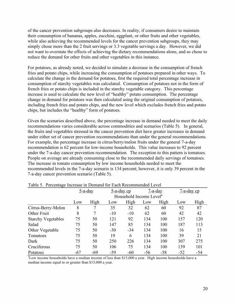
of the cancer prevention subgroups also decreases. In reality, if consumers desire to maintain their consumption of bananas, apples, zucchini, eggplant, or other fruits and other vegetables, while also achieving the recommended levels for the cancer prevention subgroups, they may simply chose more than the 2 fruit servings or 3.3 vegetable servings a day. However, we did not want to overstate the effects of achieving the dietary recommendations alone, and so chose to reduce the demand for other fruits and other vegetables in this instance. For potatoes, as already noted, we decided to simulate a decrease in the consumption of french fries and potato chips, while increasing the consumption of potatoes prepared in other ways. To calculate the change in the demand for potatoes, first the required total percentage increase in consumption of starchy vegetables was calculated. Consumption of potatoes not in the form of french fries or potato chips is included in the starchy vegetable category. This percentage increase is used to calculate the new level of “healthy” potato consumption. The percentage change in demand for potatoes was then calculated using the original consumption of potatoes, including french fries and potato chips, and the new level which excludes french fries and potato chips, but includes the “healthy” form of potatoes. Given the scenarios described above, the percentage increase in demand needed to meet the daily recommendations varies considerable across commodities and scenarios (Table 5). In general, the fruits and vegetables stressed in the cancer prevention diet have greater increases in demand under either set of cancer prevention recommendations than under the general recommendations. For example, the percentage increase in citrus/berry/melon fruits under the general 7-a-day recommendation is 62 percent for low-income households. This value increases to 92 percent under the 7-a-day cancer prevention recommendation. The exception to this pattern is tomatoes. People on average are already consuming close to the recommended daily servings of tomatoes. The increase in tomato consumption by low income households needed to meet the recommended levels in the 7-a-day scenario is 134 percent; however, it is only 39 percent in the 7-a-day cancer prevention scenario (Table 5). Table 5. Percentage Increase in Demand for Each Recommended Level 5-a-day 5-a-day cp 7-a-day 7-a-day cp Household Income Levela

Low High Low High Low High Low High Citrus-Berry-Melon 8 7 35 32 62 60 92 87 Other Fruit 8 7 -10 -10 62 60 42 42 Starchy Vegetables 75 50 121 92 134 100 157 120 Salad 75 50 147 85 134 100 187 113 Other Vegetable 75 50 -30 -34 134 100 16 15 Tomatoes 75 50 19 6 134 100 39 21 Dark 75 50 250 226 134 100 307 275 Cruciferous 75 50 106 75 134 100 139 101 Potatoes -67 -69 -59 -60 -56 -58 -52 -54 aLow income households have a median income of less than $15,000 a year. High income households have a median income equal to or greater than $15,000 a year.

21

The calculations of the change in prices, final demand, production, and trade were done assuming two different supply elasticities. The first assumes that growers, importers, exporters, and marketing firms have a low supply elasticity and are relatively less responsive to the changes in prices. The second assumes that they have larger supply elasticities and are relatively more responsive to changes in prices. Two supply response scenarios are used because there are very few studies that have calculated the supply elasticity of individual fruits and vegetables, and none that have done so using a complete model of U.S. horticultural industries. The values used in this analysis have been extrapolated from the few available studies on individual commodities to represent a reasonable range of elasticities, given the agro-climatic conditions in California and the rest of the U.S. With four demand scenarios and two supply response assumptions, eight simulations are used to measure the costs and benefits of Californians eating more fruits and vegetables. A sensitivity analysis was also done using different demand elasticities; however, there was very little change in the surplus measurements and no change in the qualitative results.

22

DATA Biennial consumption data by Californians for the years 1993 to 1999 were provided by the California Department of Health Services, Cancer Prevention and Nutrition Section. The data include information on the average daily servings of individual fruits and vegetables by income group. U.S. and California production and farm value data are available from the USDA’s Fruit and Nut Yearbook and Outlook reports, the Vegetable and Melon Yearbook and Outlook reports, and Agricultural Statistics. The USDA data has California statistics for most, but not all crops. Additional data for California are available from the California Agricultural Statistics Service (1998-2002). Data on agricultural inputs used in the production of individual commodities are available from crop budgets prepared by the University of California Cooperative Extension. The consumption, production, and agricultural input data used in the analysis are presented in Appendix II. Important parameters needed for this study are the elasticities of demand and supply. Demand elasticities for many of the fruit and vegetables included in this study are available in Huang (1993). The Huang data are used to determine an own-price and cross-price elasticity of demand for each commodity. The data and methodology used to calculate the cross-price elasticity of demand are in Appendix I. Supply elasticities for individual fruits and vegetables are extrapolated from the literature. The supply elasticities are determined for three different production groups. The first group includes all row vegetables, the second is all row fruits (melons and strawberries), and the final group is the perennial tree and vine fruit crops. These three groups are chosen based on the agro-climatic distribution of crops grown in California and how the crop is grown. Row vegetables are grown mainly in the Salinas Valley along California’s north-central coast, with significant winter vegetable production in the Imperial Valley, located inland in southern California. Because there are few agro-climatic regions with significant vegetable production, and most of the land that can produce vegetable crops in the Salinas Valley is already planted in vegetables, there are few options to expand production, and the supply response would be relatively inelastic (i.e., less responsive to changes in prices). The own-price supply elasticities are set equal to 0.5 for the less responsive scenario and 1.0 for the more responsive scenario. Melons are grown throughout California’s Central valley and in the Imperial Valley, and there is significant strawberry production along California’s coast. Because there is a significant amount of land in other crops in these regions, the supply response to changes in the price of row fruits would be more elastic than for row vegetable crops. The own-price supply elasticities for row fruits are set to 1.0 for the less responsive scenario and 1.5 for the more responsive scenario. Significant costs are associated with moving perennial crops in and out of production, and so a lower supply elasticity than for row fruits is used. However, production of perennial crops occurs throughout the Central Valley; therefore, the elasticity should be greater than for row vegetables. The two own-price supply elasticities for perennial crops are set to 0.75 and 1.25.

23

The data and methodology used to calculate the cross-price elasticities of supply are in Appendix I.

24

RESULTS The percentage changes in market and grower prices, market supply, trade, consumption, and production are the solutions to the system of equations that characterize our market model. As expected, under all scenarios, an increase in the demand for fruits and vegetables causes both market and grower prices to increase. Higher prices cause the final market equilibrium quantity to increase from an increase in imports, a decrease in exports, and greater production by growers in California and in the rest of the U.S. Depending upon the substitution effects, consumption of some fruits and vegetables may be greater than the initial shift in demand, while the consumption of other fruits and vegetables may be less. How prices, market supply, consumption and production change differs according to how demand changes, how consumers and producers react to price changes, and trade patterns. These differences in turn cause differences in estimates of the costs and benefits from greater consumption of fruits and vegetables. Percentage Change in Final Prices, Final Market Equilibrium Quantity and Trade 5-a-day All prices increase following the increase in demand for fruits and vegetables; however, the amount that prices increase varies (Table 6). For fruit, the price increase for plums and prunes is the smallest at 0.32 percent. This price increase is similar under both supply response scenarios. The greatest increase in price is for strawberries at 0.74 percent when supply elasticities are less responsive to price changes and at 0.97 percent when supply elasticities are more responsive. For melons, we also observe that as the supply elasticity becomes larger, market prices are higher. Based on the single-market diagram showing supply and demand (Figure 1), such an outcome seems counterintuitive. The less responsive is supply, the greater should be the price increase. However, that intuition is based on a single demand shift (say for strawberries) and a single market. The supply curve for a good such as strawberries is drawn holding constant the prices of other goods; the movement up a single supply curve reflects producers’ response to the increase in demand for strawberries. When commodities are substitutes in production, producers may adjust away from the production of certain commodities by enough to cause the change in market supply to be lower, and market price to increase. The supply elasticity for this strawberries and melons is the most responsive, and these commodities also have a large number of other commodities that are substitutes in production. Therefore, growers can move resources in and out of melon and strawberry production more easily and into the production of crops, such as vegetables, where the shift in demand is higher. For all other commodities, the price increase is lower, and output greater, when the supply elasticities are more responsive. The cross-price demand effects would then further cause the quantity demanded to decrease and market prices to rise as consumers substitute away from the higher priced strawberries and melons, and into commodities with smaller price increases. Recall that the current gap between actual and recommended servings is greater for vegetables than for fruit. Therefore, our simulations involve a larger increase in quantity demanded for vegetables, and the price increase for vegetables is greater than for fruit (Table 6). Even though

25

Table 6. Percentage Change in the U.S. market variables for the 5-a-day scenario. Price Quantity Trade Price Quantity Trade Less Responsive More Responsive Citrus-Berry-Melon Cantaloupe 0.54 0.77 1.09 0.61 0.75 1.22 Grapefruit 0.44 0.83 -0.89 0.44 0.83 -0.87 Honeydews 0.57 0.77 1.15 0.65 0.74 1.3 Oranges 0.64 0.58 1.29 0.63 0.6 1.26 Strawberries 0.74 0.7 -1.48 0.97 0.61 -1.94 Tangerines and other citrus 0.65 0.74 -1.29 0.63 0.75 -1.26 Watermelon 0.64 0.73 1.27 0.71 0.71 1.42 Other Fruit Apple 0.67 0.77 1.34 0.65 0.78 1.29 Apricots 0.64 0.75 -1.27 0.62 0.76 -1.25 Avocados 0.61 0.75 1.22 0.6 0.76 1.21 Bananas 0.44 0.89 0.89 0.44 0.89 0.89 Cherries 0.52 0.8 -1.05 0.52 0.81 -1.03 Grapes 0.71 0.68 1.43 0.7 0.69 1.4 Peaches & Nectarines 0.65 0.72 -1.3 0.64 0.73 -1.27 Pears 0.61 0.76 -1.21 0.59 0.77 -1.19 Pineapples 0.5 0.87 0.99 0.5 0.87 1 Plums and prunes 0.32 0.88 -0.63 0.32 0.88 -0.64 Starchy Vegetables Corn, Fresh Market Sweet 5.49 5.07 -10.97 5.11 5.11 -10.23 Sweet Potatoes 5.93 4.83 -11.85 5.45 4.88 -10.9 Salad Lettuce, All 5.73 5.24 -11.45 5.25 5.28 -10.5 Other Vegetable Artichokes 4.02 5.23 8.05 3.89 5.22 7.78 Asparagus 4.34 5.22 8.68 4.29 5.18 8.57 Beans, Snap 5.79 5.06 11.59 5.53 5.07 11.07 Celery 5.54 5.5 -11.08 5.09 5.54 -10.17 Cucumbers 4.61 5.51 9.21 4.42 5.51 8.84 Eggplant 4.52 5.13 9.03 4.32 5.13 8.64 Onions 6.37 4.95 -12.73 5.82 5.03 -11.63 Peas 5.38 4.2 10.77 5.05 4.27 10.1 Peppers, Bell 5.51 5 11.02 5.14 5.03 10.29 Tomatoes Tomatoes, Fresh Market 4.23 4.48 8.45 4.03 4.5 8.05 Tomatoes, Processing 5.42 5.21 -10.84 5.25 5.21 -10.5 Dark Carrots 5.73 4.08 11.47 5.28 4.22 10.55 Spinach 5.57 5.06 -11.13 5.13 5.11 -10.25 Broccoli 6.02 4.98 12.04 5.55 5.04 11.1 Cruciferous Cabbage 7.26 4.87 -14.51 6.47 4.99 -12.94 Cauliflower 4.63 5.21 -9.26 4.29 5.23 -8.57 Potatoes Potatoes -2.2 -7.02 4.4 -2.08 -7.05 4.16

26

the price increase is higher for vegetables, when supply elasticities are less responsive the change in price ranges from a low of 4.02 percent for artichokes to a high of 7.26 percent for cabbage. When supply elasticities are more responsive, prices increase by a smaller amount. The percentage increase in prices for artichokes is now only 3.89 and 6.47 for cabbage. The increase in prices appears to be much lower than the shift in quantity demanded by Californians. This is because it is the percentage change in quantity demanded for the entire U.S. that determines U.S. prices. California has only 12 percent of the U.S. population. This makes the shift in demand for the U.S. market to be about 12 percent of the shift in demand by Californians, so that a 100 percent increase in demand by Californians translates into only a 12 percent increase in demand at the national level. Therefore, even though the change in demand by Californians for fruit under the 5-a-day general recommendation is eight percent for low-income families and seven percent for high income families, the change in demand for the overall U.S. fruit market is less than one percent. For vegetables, the increase in demand by Californians of 75 percent for low-income families and 50 percent for high income families translates into a shift in demand for the entire U.S of about nine percent for low income families and six percent for high income. Trade also has an impact on the final change in market prices and supply. Whether the increased U.S. market supply is coming primarily from changes in trade patterns, or from increases in production depends upon the commodity. For a commodity such as bananas, almost all of the U.S. supply is imported from other countries, so changes in trade account for most of the increase in U.S. supply. On the other hand, for commodities such as cabbage or strawberries, very little is traded with other markets and increased quantities must come from domestic production. The percentage change in trade is smallest for the commodities with the largest quantities traded, and largest for commodities with almost no trade. Imports of bananas increase by 0.89 percent while strawberry exports decrease by 1.94 percent and cabbage exports by 12.94 percent. Even though the percentage change in trade by subgroup is greatest for cabbage in the vegetable category and strawberries in the fruit category, because there is so little traded in these commodities, most of the increase in U.S. market supply is coming from greater production within California and the rest of the U.S. The percentage change in price is also smallest for the commodities with the largest quantities traded. Bananas have a price increase of zero under both supply response scenarios. Cabbage and strawberries are the commodities with the highest price increases, and the greatest differences in price between the two supply response scenarios (Table 6). For vegetables, the commodities with price increases below five percent are the top ranked commodities for net imports and net exports (Table 4). 5-a-day cancer prevention With the 5-a-day cancer prevention scenario, because we are holding total consumption to 5 fruits and vegetables a day, consumption of fruit and vegetables in the “other” category needs to

27

decrease in order to achieve the recommendations for the cancer prevention diet while also restricting total fruit and vegetable consumption to the 5-a-day target (Table 7). As expected, market prices fall when quantity demanded decreases, and rise when quantity demanded increases. The direction of change in final market supply is the same as the direction of change in prices. Market supply increases when prices increase, and decreases when prices decrease (Table 7). With a greater increase in quantity demanded for the fruits and vegetables emphasized in the cancer prevention recommendations, there are greater increases in prices for those items than under the general 5-a-day recommendations. For example, when the supply elasticities are less responsive, the increase in the price of oranges under the 5-a-day scenario is about 0.64 percent. For the cancer prevention scenario, the increase is 2.07 percent. For broccoli, the increase in price under the 5-a-day recommendation is only 6.02 percent, but a much larger 24.69 percent for the cancer prevention recommendation. As was the case with the 5-a-day general recommendation, when the supply elasticities are more responsive, the absolute value of the change in price is lower for all commodities except cantaloupes, honeydew melons, and strawberries. Trade also has a significant impact on the magnitude of the price changes in the 5-a-day cancer prevention program. The commodities with the highest proportion of market supply traded within the cancer prevention sub-groups have the lowest increase in prices within those groups (Table 7). For example, cauliflower has a higher share of production exported than cabbage (Table 4). When supply elasticities are less responsive, prices increase by 6.81 percent for cauliflower and 10.61 percent for cabbage. A larger share of U.S. market supply is imported for plums and prunes than for peaches and nectarines (Table 5). When supply elasticities are less responsive the decrease in price is 0.25 percent for plums and prunes, and 0.51 percent for peaches and nectarines. While small, the absolute value of the percentage change is price for peaches and nectarines is twice as large as the change for plums and prunes. 7-a-day The results for the 7-a-day recommendations are qualitatively the same as the results of the 5-a-day recommendation, except that the magnitudes of the changes are greater (Table 8). Instead of the price changes for fruit all being less than one percent, the price changes are now between 2.65 percent for plums and prunes when supply elasticities are less responsive, and 6.22 percent for strawberries when they are more responsive. For vegetables, the change in prices is between 7.86 for artichokes and 12.61 for onions when supply elasticities are more responsive. Potatoes are the exception. Because there is greater consumption of starchy vegetables under the 7-a-day general scenario, the decrease in quantity demanded is less than for the 5-a-day scenario. Consequently, the decrease in potato prices is less. Again, when supply elasticities are more responsive, the percentage change in price will be lower, and the percentage change in quantity will be higher than when supply elasticities are less responsive, except for cantaloupe, honeydew melons, and strawberries. With the larger shifts in demand, watermelon is no longer an exception. Watermelon is also the fruit with the lowest share

28

Table 7. Percentage Change in the U.S. market variables for the 5-a-day cancer prevention scenario. Price Quantity Trade Price Quantity Trade Less Responsive More Responsive Citrus-Berry-Melon Cantaloupe 2.03 2.9 4.05 2.04 2.89 4.09 Grapefruit 1.63 3.04 -3.27 1.55 3.07 -3.11 Honeydews 2.14 2.89 4.28 2.16 2.88 4.32 Oranges 2.07 1.89 4.14 1.96 1.99 3.93 Strawberries 2.7 2.67 -5.4 2.76 2.65 -5.51 Tangerines and other citrus 2.4 2.76 -4.8 2.26 2.81 -4.52 Watermelon 2.37 2.75 4.75 2.33 2.76 4.66 Other Fruit Apple -0.72 -0.83 -1.44 -0.68 -0.85 -1.36 Apricots -0.5 -0.64 1 -0.46 -0.66 0.92 Avocados -0.42 -0.54 -0.83 -0.4 -0.56 -0.79 Bananas -0.32 -0.65 -0.65 -0.33 -0.65 -0.65 Cherries -0.44 -0.67 0.87 -0.41 -0.68 0.82 Grapes -0.43 -0.47 -0.87 -0.4 -0.5 -0.8 Peaches & Nectarines -0.51 -0.61 1.03 -0.47 -0.63 0.95 Pears -0.49 -0.63 0.99 -0.46 -0.65 0.93 Pineapples -0.41 -0.71 -0.81 -0.41 -0.71 -0.81 Plums and prunes -0.25 -0.74 0.49 -0.23 -0.75 0.45 Starchy Vegetables Corn, Fresh Market Sweet 9.68 8.94 -19.35 8.87 9.05 -17.75 Sweet Potatoes 10.58 8.61 -21.15 9.65 8.75 -19.29 Salad Lettuce, All 9.83 9 -19.66 9.03 9.07 -18.07 Other Vegetable Artichokes -2.01 -2.64 -4.02 -1.89 -2.73 -3.79 Asparagus -2.15 -2.6 -4.3 -2.07 -2.69 -4.14 Beans, Snap -2.76 -2.41 -5.52 -2.67 -2.5 -5.33 Celery -2.9 -2.92 5.8 -2.57 -2.99 5.13 Cucumbers -2.08 -2.49 -4.15 -2 -2.57 -4.01 Eggplant -2.27 -2.58 -4.54 -2.18 -2.67 -4.36 Onions -3 -2.34 6 -2.53 -2.5 5.06 Peas -1.46 -1.14 -2.92 -1.44 -1.3 -2.89 Peppers, Bell -2.67 -2.43 -5.34 -2.48 -2.54 -4.96 Tomatoes Tomatoes, Fresh Market 1.65 1.74 3.29 1.5 1.67 2.99 Tomatoes, Processing 1.17 1.12 -2.33 1.1 1.08 -2.21 Dark Carrots 21.42 15.28 42.83 19.68 16.05 39.36 Spinach 22.85 20.78 -45.7 20.91 21.15 -41.82 Broccoli 24.69 20.48 49.39 22.57 20.87 45.14 Cruciferous Cabbage 10.61 7.12 -21.23 9.54 7.28 -19.09 Cauliflower 6.81 7.67 -13.63 6.36 7.7 -12.71 Potatoes Potatoes -1.89 -6.02 3.77 -1.78 -6.06 3.55

29

Table 8. Percentage Change in the U.S. market variables for the 7-a-day scenario. Price Quantity Trade Price Quantity Trade Less Responsive More Responsive Citrus-Berry-Melon Cantaloupe 4.61 6.61 9.23 4.64 6.58 9.27 Grapefruit 3.79 7.07 -7.58 3.7 7.04 -7.4 Honeydews 4.87 6.59 9.74 4.89 6.56 9.79 Oranges 5.46 4.98 10.93 5.27 5.07 10.54 Strawberries 6.14 6.08 -12.28 6.22 6.03 -12.45 Tangerines and other citrus 5.38 6.19 -10.76 5.2 6.26 -10.39 Watermelon 5.4 6.24 10.79 5.27 6.28 10.54 Other Fruit Apple 5.69 6.57 11.38 5.47 6.57 10.95 Apricots 5.36 6.45 -10.71 5.19 6.5 -10.38 Avocados 5.18 6.46 10.36 5.07 6.49 10.14 Bananas 3.78 7.55 7.56 3.75 7.48 7.49 Cherries 4.47 6.83 -8.93 4.36 6.85 -8.73 Grapes 5.99 5.87 11.97 5.78 5.92 11.56 Peaches & Nectarines 5.47 6.16 -10.95 5.29 6.22 -10.59 Pears 5.14 6.43 -10.27 4.98 6.48 -9.97 Pineapples 4.21 7.38 8.43 4.2 7.36 8.41 Plums and prunes 2.65 7.49 -5.31 2.65 7.47 -5.3 Starchy Vegetables Corn, Fresh Market Sweet 10.92 10.1 -21.85 10.22 10.16 -20.43 Sweet Potatoes 11.93 9.71 -23.86 11 9.82 -22 Salad Lettuce, All 11.38 10.4 -22.76 10.49 10.47 -20.98 Other Vegetable Artichokes 8.11 10.53 16.22 7.86 10.5 15.71 Asparagus 8.71 10.47 17.43 8.63 10.4 17.25 Beans, Snap 11.5 10.04 23 11.01 10.05 22.02 Celery 10.89 10.8 -21.78 10.05 10.85 -20.1 Cucumbers 9.03 10.8 18.06 8.68 10.78 17.37 Eggplant 9.09 10.33 18.19 8.71 10.32 17.43 Onions 12.61 9.81 -25.21 11.57 9.95 -23.13 Peas 10.82 8.44 21.65 10.18 8.59 20.37 Peppers, Bell 11 9.98 22.01 10.31 10.04 20.61 Tomatoes Tomatoes, Fresh Market 8.47 8.98 16.95 8.1 9.01 16.19 Tomatoes, Processing 10.75 10.34 -21.5 10.43 10.33 -20.86 Dark Carrots 11.47 8.16 22.93 10.6 8.42 21.2 Spinach 11.07 10.05 -22.15 10.24 10.15 -20.48 Broccoli 11.99 9.9 23.97 11.1 10 22.2 Cruciferous Cabbage 14.32 9.6 -28.63 12.83 9.83 -25.65 Cauliflower 9.26 10.39 -18.52 8.62 10.44 -17.25 Potatoes Potatoes -1.76 -5.61 3.52 -1.6 -5.67 3.2

30

of market supply that is imported (Table 4) and, therefore, has a comparatively higher percentage change in market prices compared to other melons. 7-a-day cancer prevention The results of the 7-a-day cancer prevention recommendation are qualitatively different from the 5-a-day cancer prevention recommendations. Because quantity demanded increases for all commodities, prices increase, market supply increases, imports increase and exports decrease for all commodities. It is also no longer the case that supply of melons and strawberries declines enough so that prices rise when grower response is more elastic (Table 9). Now some crops have both lower market prices and supply, different crops have a smaller increase in quantity supplied and a greater increase in prices, while the remaining have lower prices and greater supply. When the supply elasticities are more responsive, both lower prices and a lower market supply are observed for cantaloupes, grapefruit, honeydews, apples, bananas, cherries, pineapples, snap beans, celery, cucumbers, eggplant, peas, bell peppers, and fresh and processed tomatoes (Table 9). The crops that now have a greater increase in market prices, and a smaller increase in market supply when the supply elasticities are more responsive are plums and prunes, asparagus, and onions. In general, all these crops also have the lowest percentage increase in prices. The crops that have the lower market prices and higher quantity supplied are the crops in the cancer prevention sub-groups with the largest shift in quantity demanded. These sub-groups are the salad, dark, and cruciferous vegetables, and the citrus/melon/berry fruit sub-groups. However, only the citrus/berry/melon crops with the highest change in market prices (oranges, tangerines and other citrus, and watermelon) also have lower prices and greater market quantity when the supply elasticities are more responsive. Consumer Demand - California In addition to the initial shift in quantity demanded, two factors drive the final adjustments in consumption of fruits and vegetables. The first is the increase in the price of a commodity, and the second is the increase in the price of substitutes in consumption. In this study fruits are considered to be substitutes in consumption for each other while vegetables are substitutes for each other. If the price of one commodity increases more rapidly than the price of a second, then it is possible that consumption of the second commodity will increase, even though its price has also increased. 5-a-day For all fruit commodities the final change in consumption by Californians in both low and high income households is within one percent of the initial shift in quantity demanded needed to meet the recommendations for the 5-a-day scenario under both supply response assumptions (Table 10). For vegetables, the final change in demand by Californians under both supply response scenarios is within 1.5 percent of the original shift in quantity demanded. Due to the increase in

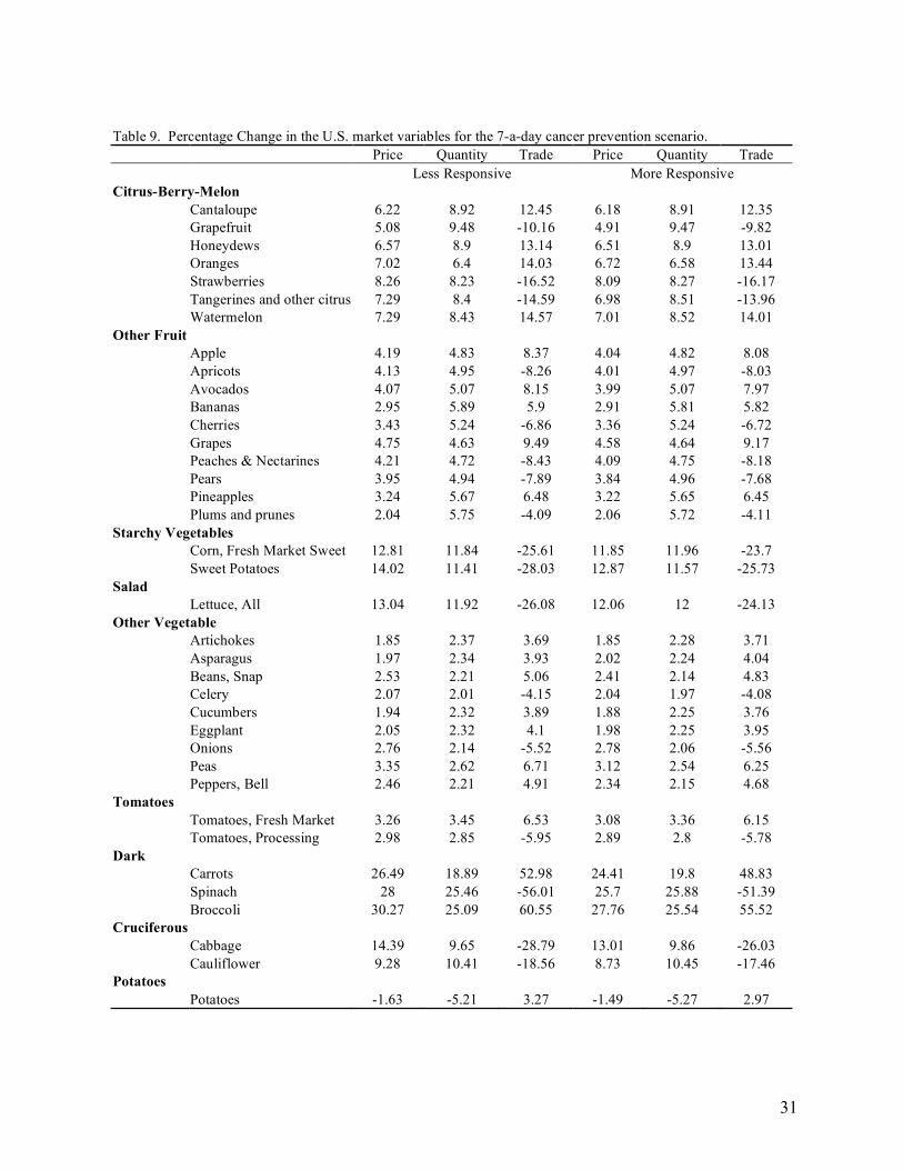
31

Table 9. Percentage Change in the U.S. market variables for the 7-a-day cancer prevention scenario. Price Quantity Trade Price Quantity Trade Less Responsive More Responsive Citrus-Berry-Melon Cantaloupe 6.22 8.92 12.45 6.18 8.91 12.35 Grapefruit 5.08 9.48 -10.16 4.91 9.47 -9.82 Honeydews 6.57 8.9 13.14 6.51 8.9 13.01 Oranges 7.02 6.4 14.03 6.72 6.58 13.44 Strawberries 8.26 8.23 -16.52 8.09 8.27 -16.17 Tangerines and other citrus 7.29 8.4 -14.59 6.98 8.51 -13.96 Watermelon 7.29 8.43 14.57 7.01 8.52 14.01 Other Fruit Apple 4.19 4.83 8.37 4.04 4.82 8.08 Apricots 4.13 4.95 -8.26 4.01 4.97 -8.03 Avocados 4.07 5.07 8.15 3.99 5.07 7.97 Bananas 2.95 5.89 5.9 2.91 5.81 5.82 Cherries 3.43 5.24 -6.86 3.36 5.24 -6.72 Grapes 4.75 4.63 9.49 4.58 4.64 9.17 Peaches & Nectarines 4.21 4.72 -8.43 4.09 4.75 -8.18 Pears 3.95 4.94 -7.89 3.84 4.96 -7.68 Pineapples 3.24 5.67 6.48 3.22 5.65 6.45 Plums and prunes 2.04 5.75 -4.09 2.06 5.72 -4.11 Starchy Vegetables Corn, Fresh Market Sweet 12.81 11.84 -25.61 11.85 11.96 -23.7 Sweet Potatoes 14.02 11.41 -28.03 12.87 11.57 -25.73 Salad Lettuce, All 13.04 11.92 -26.08 12.06 12 -24.13 Other Vegetable Artichokes 1.85 2.37 3.69 1.85 2.28 3.71 Asparagus 1.97 2.34 3.93 2.02 2.24 4.04 Beans, Snap 2.53 2.21 5.06 2.41 2.14 4.83 Celery 2.07 2.01 -4.15 2.04 1.97 -4.08 Cucumbers 1.94 2.32 3.89 1.88 2.25 3.76 Eggplant 2.05 2.32 4.1 1.98 2.25 3.95 Onions 2.76 2.14 -5.52 2.78 2.06 -5.56 Peas 3.35 2.62 6.71 3.12 2.54 6.25 Peppers, Bell 2.46 2.21 4.91 2.34 2.15 4.68 Tomatoes Tomatoes, Fresh Market 3.26 3.45 6.53 3.08 3.36 6.15 Tomatoes, Processing 2.98 2.85 -5.95 2.89 2.8 -5.78 Dark Carrots 26.49 18.89 52.98 24.41 19.8 48.83 Spinach 28 25.46 -56.01 25.7 25.88 -51.39 Broccoli 30.27 25.09 60.55 27.76 25.54 55.52 Cruciferous Cabbage 14.39 9.65 -28.79 13.01 9.86 -26.03 Cauliflower 9.28 10.41 -18.56 8.73 10.45 -17.46 Potatoes Potatoes -1.63 -5.21 3.27 -1.49 -5.27 2.97

32

Table 10. Percentage change in California consumption for the 5-a-day scenario. Household Income Groupa

Low High Low High Low High Original Shift Less Responsive More Responsive Citrus-Berry-Melon Cantaloupe 8.1 7.0 8.08 7.00 8.05 6.97 Grapefruit 8.1 7.0 8.13 7.04 8.12 7.05 Honeydews 8.1 7.0 8.07 6.99 8.04 6.97 Oranges 8.1 7.0 7.86 6.81 7.87 6.82 Strawberries 8.1 7.0 8.00 6.92 7.91 6.83 Tangerines and other citrus 8.1 7.0 8.04 6.97 8.05 6.98 Watermelon 8.1 7.0 8.04 6.96 8.01 6.93 Other Fruit Apple 8.1 7.0 8.08 6.99 8.08 6.99 Apricots 8.1 7.0 8.04 6.97 8.05 6.98 Avocados 8.1 7.0 8.04 6.97 8.05 6.98 Bananas 8.1 7.0 8.19 7.11 8.18 7.11 Cherries 8.1 7.0 8.09 7.02 8.10 7.02 Grapes 8.1 7.0 7.98 6.91 7.99 6.91 Peaches & Nectarines 8.1 7.0 8.02 6.94 8.03 6.95 Pears 8.1 7.0 8.05 6.98 8.06 6.99 Pineapples 8.1 7.0 8.17 7.09 8.17 7.09 Plums and prunes 8.1 7.0 8.17 7.10 8.18 7.10 Starchy Vegetables Corn, Fresh 75.2 49.7 74.55 49.11 74.59 49.14 Sweet Potatoes 75.2 49.7 74.45 49.01 74.51 49.06 Salad Lettuce, All 75.2 49.7 74.76 49.27 74.80 49.31 Other Vegetable Artichokes 75.2 49.7 74.86 49.42 74.85 49.40 Asparagus 75.2 49.7 74.80 49.35 74.76 49.32 Beans, Snap 75.2 49.7 74.48 49.04 74.49 49.05 Celery 75.2 49.7 74.83 49.36 74.86 49.39 Cucumbers 75.2 49.7 74.74 49.30 74.73 49.29 Eggplant 75.2 49.7 74.76 49.31 74.76 49.31 Onions 75.2 49.7 74.38 48.94 74.46 49.01 Peas 75.2 49.7 73.66 48.26 73.74 48.33 Peppers, Bell 75.2 49.7 74.53 49.08 74.57 49.12 Tomatoes Tomatoes, Fresh Market 75.2 49.7 73.85 48.50 73.88 48.51 Tomatoes, Processing 75.2 49.7 74.65 49.20 74.65 49.19 Dark Carrots 75.2 49.7 73.50 48.12 73.64 48.26 Spinach 75.2 49.7 74.51 49.07 74.56 49.12 Broccoli 75.2 49.7 74.43 48.99 74.49 49.05 Cruciferous Cabbage 75.2 49.7 75.2 48.73 74.29 48.85 Cauliflower 75.2 49.7 75.2 49.29 74.76 49.32 Potatoes Potatoes -67.1 -68.6 -66.61 -68.09 -66.64 -68.12 aLow income households have a median income of less than $15,000 a year. High income households have a median income equal to or greater than $15,000 a year.

33

prices, the consumption of most commodities is less than the increase in consumption needed to meet the 5-a-day recommendations. However, because people can substitute goods for one another in consumption, the consumption of some commodities increases, even though their prices are higher. In addition, people will substitute into the consumption of potatoes because the price falls for this commodity as quantity demanded declines. High-income consumers, who eat a wider variety of fruits and vegetables than lower income consumers, also have more flexibility in switching consumption. High-income consumers increase consumption of grapefruit, bananas, cherries, pineapples, plums and prunes (Table 10). Low-income consumers already concentrate consumption in the lower priced commodities, and so have less flexibility in choosing which items to shift into. Low-income consumers only shift consumption into grapefruit, bananas, pineapples, and plums and prunes. The shift in consumption toward commodities with lower price increases is only seen within the fruit category. For vegetables, the increase in prices is sufficiently large enough that it hinders people from switching consumption into the vegetables with relatively low price increases. In comparing the changes in consumption based on supply responsiveness, when the supply elasticities become more responsive, consumption off all items, except berries and melons, are higher. For berries and melons the increase in consumption is lower. This is because the price for all commodities, except berries and melons, increases by a smaller amount when the supply elasticities are less responsive. 5-a-day cancer prevention With the cancer prevention recommendations, quantity demanded for the cancer prevention sub-groups increases, while it decreases for the “other” fruit and “other” vegetable categories. Because of this, prices of the cancer prevention subgroups rise while prices for the “other” subgroups fall. Therefore, consumption of most of the cancer prevention fruits and vegetables is slightly lower than the recommended increase in quantity demanded. For example, the increase in consumption needed to meet the 0.5 recommended daily servings of cruciferous vegetables is 105.6 percent for low-income consumers and 74.7 percent for high-income consumers. The final change in consumption for cauliflower is about 104.78 to 104.82 percent for low-income consumers and 74 percent for high-income consumers. On the other hand, the decrease in consumption of “other” fruits and vegetables is not as great as the initial shift down in quantity demanded (Table 11). People substitute into the consumption of “other” fruit and vegetables, and also tomatoes. Tomatoes are the sub-category with the smallest percentage increase in quantity demanded needed to meet the cancer prevention recommendations. The shift in quantity demanded is only 19.3 percent for low-income consumers and 5.6 percent for high income. So even though prices are increasing for tomatoes, people will substitute into more tomato consumption due to the relatively higher increase in prices for the remaining cancer prevention commodities.

34

Table 11. Percentage change in California consumption for the 5-a-day cancer prevention scenario. Household Income Groupa Low High Low High Low High Original Shift Less Responsive More Responsive Citrus-Berry-Melon Cantaloupe 35.0 31.9 34.35 31.27 34.34 31.26 Grapefruit 35.0 31.9 34.47 31.39 34.50 31.42 Honeydews 35.0 31.9 34.33 31.27 34.32 31.25 Oranges 35.0 31.9 33.27 30.25 33.37 30.35 Strawberries 35.0 31.9 34.09 31.01 34.06 30.99 Tangerines and other citrus 35.0 31.9 34.22 31.16 34.28 31.21 Watermelon 35.0 31.9 34.20 31.14 34.22 31.15 Other Fruit Apple -9.8 -10.0 -9.55 -9.73 -9.57 -9.75 Apricots -9.8 -10.0 -9.37 -9.53 -9.39 -9.55 Avocados -9.8 -10.0 -9.28 -9.43 -9.30 -9.45 Bananas -9.8 -10.0 -9.39 -9.54 -9.39 -9.55 Cherries -9.8 -10.0 -9.40 -9.56 -9.41 -9.57 Grapes -9.8 -10.0 -9.22 -9.36 -9.25 -9.40 Peaches & Nectarines -9.8 -10.0 -9.35 -9.51 -9.37 -9.53 Pears -9.8 -10.0 -9.37 -9.53 -9.38 -9.55 Pineapples -9.8 -10.0 -9.45 -9.61 -9.45 -9.61 Plums and prunes -9.8 -10.0 -9.47 -9.63 -9.48 -9.65 Starchy Vegetables Corn, Fresh 120.6 91.5 119.16 90.15 119.27 90.26 Sweet Potatoes 120.6 91.5 118.97 89.96 119.11 90.09 Salad Lettuce, All 146.5 85.1 145.64 84.24 145.71 84.31 Other Vegetable Artichokes -30.0 -34.3 -28.92 -33.13 -29.01 -33.22 Asparagus -30.0 -34.3 -28.89 -33.10 -28.97 -33.19 Beans, Snap -30.0 -34.3 -28.76 -32.97 -28.84 -33.06 Celery -30.0 -34.3 -29.30 -33.54 -29.37 -33.62 Cucumbers -30.0 -34.3 -28.91 -33.12 -28.99 -33.20 Eggplant -30.0 -34.3 -28.87 -33.07 -28.95 -33.16 Onions -30.0 -34.3 -28.72 -32.94 -28.87 -33.10 Peas -30.0 -34.3 -27.56 -31.64 -27.71 -31.81 Peppers, Bell -30.0 -34.3 -28.78 -32.98 -28.88 -33.09 Tomatoes Tomatoes, Fresh Market 19.3 5.6 20.08 6.63 20.03 6.55 Tomatoes, Processing 19.3 5.6 19.60 5.97 19.57 5.93 Dark Carrots 249.8 225.9 240.01 216.33 240.81 217.10 Spinach 249.8 225.9 245.44 221.63 245.81 221.99 Broccoli 249.8 225.9 245.13 221.32 245.53 221.71 Cruciferous Cabbage 105.6 74.7 103.96 73.15 104.13 73.32 Cauliflower 105.6 74.7 104.78 73.97 104.82 74.00 Potatoes Potatoes -58.5 -59.8 -57.99 -59.25 -58.03 -59.29 aLow income households have a median income of less than $15,000 a year. High income households have a median income equal to or greater than $15,000 a year.

35

7-a-day The changes in consumption are qualitatively similar to the changes in consumption under the 5-a-day scenario (Table 12). For both high and low-income consumers under both supply response scenarios, final quantity demanded is all within 1-2 percent of the original shift for fruit and 2-3 percent of the original shift for vegetables. The increase in consumption of all commodities is greater when supply elasticities are more responsive, except for the row fruits; consumers shift into the commodities with the lowest increases in prices; and high-income consumers have more flexibility in shifting consumption than low-income consumers. The main difference between the 5-a-day and 7-a-day recommendations is that with a larger increase in market prices, there are greater adjustments. For example, under the 5-a-day scenario, when the supply elasticity in less responsive, for low-income consumers the final percentage change in the consumption of peaches and nectarines is 0.04 percentage points, or 0.5 percent lower than the recommended level. Under the 7-a-day scenario, the final change in consumption is 0.58 percentage points, or 0.9 percent lower. 7-a-day cancer prevention The quantity demanded for all commodities increases, with the shift in quantity demanded for the cancer prevention subgroups greater than for the “other” fruit and vegetable subgroups. As described previously, as consumers respond to the price increase, the final increase in consumption of most of the cancer prevention commodities is smaller, and people substitute into consuming commodities with smaller price increases. Because the increase in quantity demanded for the cancer prevention sub-groups is greater than for the “other” fruit and vegetable, and tomato sub-groups, the percentage change in prices is relatively higher (Table 13). Therefore, for fruit, people transfer consumption out of citrus/berry/melon and into all “other” fruits except grapes, for which the percentage change in price is relatively high. For vegetables, people shift out of starchy, salad, dark, cruciferous, potatoes, and into the “other” vegetables and tomatoes. Because the increase in prices is less when the supply elasticities are more responsive for the 7-a-day cancer prevention scenario, the increase in consumption of fruits and vegetables is greater for all crops. The exception is grapefruit for low-income consumers. Consumption is slightly lower at 91.59 percent versus 91.60 percent when supply elasticities are less responsive.

36

Table 12. Percentage change in California consumption for the 7-a-day scenario. Household Income Groupa Low High Low High Low High Original Shift Less Responsive More Responsive Citrus-Berry-Melon Cantaloupe 62.1 60.4 61.89 60.37 61.88 60.34 Grapefruit 62.1 60.4 62.30 60.76 62.26 60.73 Honeydews 62.1 60.4 61.84 60.35 61.83 60.32 Oranges 62.1 60.4 60.05 58.77 60.14 58.86 Strawberries 62.1 60.4 61.29 59.78 61.25 59.72 Tangerines and other citrus 62.1 60.4 61.62 60.15 61.70 60.21 Watermelon 62.1 60.4 61.55 60.06 61.60 60.10 Other Fruit Apple 62.1 60.4 61.95 60.31 61.94 60.31 Apricots 62.1 60.4 61.63 60.15 61.71 60.20 Avocados 62.1 60.4 61.61 60.16 61.66 60.19 Bananas 62.1 60.4 62.82 61.30 62.75 61.24 Cherries 62.1 60.4 62.01 60.53 62.05 60.55 Grapes 62.1 60.4 61.10 59.63 61.15 59.68 Peaches & Nectarines 62.1 60.4 61.42 59.91 61.50 59.97 Pears 62.1 60.4 61.68 60.20 61.74 60.24 Pineapples 62.1 60.4 62.65 61.14 62.66 61.12 Plums and prunes 62.1 60.4 62.74 61.25 62.75 61.23 Starchy Vegetables Corn, Fresh 133.6 99.6 132.36 98.48 132.43 98.54 Sweet Potatoes 133.6 99.6 132.15 98.26 132.26 98.37 Salad Lettuce, All 133.6 99.6 132.76 98.77 132.83 98.84 Other Vegetable Artichokes 133.6 99.6 132.97 99.08 132.94 99.04 Asparagus 133.6 99.6 132.84 98.95 132.77 98.88 Beans, Snap 133.6 99.6 132.24 98.35 132.26 98.37 Celery 133.6 99.6 132.91 98.97 132.97 99.03 Cucumbers 133.6 99.6 132.77 98.89 132.76 98.87 Eggplant 133.6 99.6 132.76 98.87 132.75 98.86 Onions 133.6 99.6 132.04 98.16 132.19 98.30 Peas 133.6 99.6 130.63 96.83 130.79 96.97 Peppers, Bell 133.6 99.6 132.32 98.43 132.39 98.49 Tomatoes Tomatoes, Fresh Market 133.6 99.6 131.05 97.35 131.10 97.37 Tomatoes, Processing 133.6 99.6 132.55 98.65 132.55 98.65 Dark Carrots 133.6 99.6 130.33 96.59 130.61 96.84 Spinach 133.6 99.6 132.29 98.40 132.39 98.50 Broccoli 133.6 99.6 132.14 98.25 132.24 98.35 Cruciferous Cabbage 133.6 99.6 131.63 97.75 131.87 97.98 Cauliflower 133.6 99.6 132.72 98.84 132.77 98.88 Potatoes Potatoes -56.1 -58.1 -55.38 -57.34 -55.44 -57.39 aLow income households have a median income of less than $15,000 a year. High income households have a median income equal to or greater than $15,000 a year.

37

Table 13. Percentage change in California consumption for the 7-a-day cancer prevention scenario. Household Income Groupa Low High Low High Low High Original Shift Less Responsive More Responsive Citrus-Berry-Melon Cantaloupe 92.0 87.4 91.11 86.69 91.13 86.68 Grapefruit 92.0 87.4 91.60 87.16 91.59 87.16 Honeydews 92.0 87.4 91.04 86.67 91.06 86.67 Oranges 92.0 87.4 88.34 84.19 88.52 84.37 Strawberries 92.0 87.4 90.31 85.91 90.38 85.95 Tangerines and other citrus 92.0 87.4 90.74 86.38 90.87 86.48 Watermelon 92.0 87.4 90.65 86.28 90.76 86.37 Other Fruit Apple 42.2 42.1 42.34 42.31 42.31 42.29 Apricots 42.2 42.1 42.26 42.39 42.31 42.41 Avocados 42.2 42.1 42.33 42.50 42.35 42.50 Bananas 42.2 42.1 43.27 43.38 43.20 43.31 Cherries 42.2 42.1 42.55 42.69 42.58 42.69 Grapes 42.2 42.1 41.96 42.12 41.97 42.13 Peaches & Nectarines 42.2 42.1 42.10 42.21 42.15 42.24 Pears 42.2 42.1 42.30 42.43 42.34 42.45 Pineapples 42.2 42.1 43.06 43.17 43.06 43.14 Plums and prunes 42.2 42.1 43.12 43.24 43.11 43.20 Starchy Vegetables Corn, Fresh 157 120 155.01 118.44 155.14 118.56 Sweet Potatoes 157 120 154.75 118.18 154.92 118.34 Salad Lettuce, All 187.0 112.8 185.91 111.72 185.99 111.80 Other Vegetable Artichokes 16.4 15.0 16.97 15.70 16.89 15.61 Asparagus 16.4 15.0 16.95 15.68 16.86 15.58 Beans, Snap 16.4 15.0 16.83 15.56 16.77 15.49 Celery 16.4 15.0 16.68 15.36 16.65 15.32 Cucumbers 16.4 15.0 16.95 15.68 16.89 15.61 Eggplant 16.4 15.0 16.93 15.66 16.86 15.59 Onions 16.4 15.0 16.78 15.50 16.71 15.42 Peas 16.4 15.0 17.08 15.96 17.03 15.89 Peppers, Bell 16.4 15.0 16.84 15.56 16.78 15.50 Tomatoes Tomatoes, Fresh Market 38.9 21.4 39.53 22.38 39.45 22.27 Tomatoes, Processing 38.9 21.4 39.13 21.73 39.09 21.69 Dark Carrots 307.2 274.7 295.54 263.34 296.47 264.25 Spinach 307.2 274.7 302.04 269.66 302.47 270.08 Broccoli 307.2 274.7 301.65 269.29 302.12 269.74 Cruciferous Cabbage 139.4 100.8 137.27 98.80 137.49 99.01 Cauliflower 139.4 100.8 138.37 99.90 138.41 99.93 Potatoes Potatoes -51.7 -53.8 -51.07 -53.11 -51.11 -53.16 aLow income households have a median income of less than $15,000 a year. High income households have a median income equal to or greater than $15,000 a year.

38

Consumers in the rest of the U.S. Consumers in the rest of the U.S. are only affected by the increase in demand by Californians through changes in market prices. As was the case with California consumers however, both the price of the commodity and the price of commodities that are substitutes in consumption influence the final changes in consumption by people in the rest of the U.S. 5-a-day As was the case for California consumers, consumers in the rest of the U.S. will substitute away from those commodities with the greatest increase in prices, and toward those commodities with the smallest (Table 14). When supply elasticities are less responsive to changes in prices, high-income consumers will increase consumption of grapefruit, bananas, pineapples, plums and prunes, cherries, and potatoes. Low-income consumers will increase consumption of grapefruit, bananas, pineapples, plum and prunes, and potatoes. The increase in potatoes is coming from the fall in their prices due to the decrease in demand by Californians. The consumption of the remaining commodities falls. Just how much consumption falls depends on the magnitude of the change in prices and the elasticity of demand. The more responsive consumers are to prices, and the greater the price change, the more consumption will fall. When supply elasticities are less responsive, the increase in the retail price of strawberries is 0.74 percent, 0.71 percent for grapes, and 0.64 percent for oranges (Table 5). The decrease in consumption by low-income consumers is 0.10 percent for strawberries, 0.12 percent for grapes and 0.25 percent for oranges (Table 14). Strawberries have an own-price elasticity of 0.42, grapes 0.59 and oranges 0.85 (see Table A.1 in the appendix). While the price increase for apples is relatively large, 0.67 percent, the change in consumption is only 0.02 percent due to a demand elasticity of only –0.1902. Even though the decline in orange consumption is 12 times the decline in apple consumption, the decline in fruit consumption is less than one percent for all fruits and most vegetables. Only peas, fresh tomatoes, and cabbage have declines in consumption that are greater than one percent. Low-income consumers decrease their consumption of fruits and vegetables by a greater amount than the decrease by high-income consumers. This is due to the income effect that higher food prices have on household budgets. Low-income consumers spend a larger share of their income on food, and changes in food prices affect their ability to purchase fruits and vegetables to a greater extent than for high-income consumers. Therefore, increases in food prices will be met with larger declines in quantity demanded by low-income consumers. Income effects are incorporated into the model through the cross-price elasticities of demand. Details are presented in Appendix I. Low-income consumers in California would experience the same income effects. When supply elasticities are more responsive, consumption of fruits and vegetables does not decrease by as much, except for melons and strawberries. Because the change in prices is not as great, consumption does not fall by as much as when the supply elasticities are less responsive.

39

Table 14. Percentage change in the rest of the U.S. consumption for the 5-a-day scenario. Household Income Groupa Low High Low High Less Responsive More Responsive Citrus-Berry-Melon Cantaloupe -0.02 0.00 -0.05 -0.03 Grapefruit 0.03 0.04 0.02 0.05 Honeydews -0.03 -0.01 -0.06 -0.03 Oranges -0.24 -0.19 -0.23 -0.18 Strawberries -0.10 -0.08 -0.19 -0.17 Tangerines and other citrus -0.06 -0.03 -0.05 -0.02 Watermelon -0.06 -0.04 -0.09 -0.07 Other Fruit Apple -0.02 -0.01 -0.02 -0.01 Apricots -0.06 -0.03 -0.05 -0.02 Avocados -0.06 -0.03 -0.05 -0.02 Bananas 0.09 0.11 0.08 0.11 Cherries -0.01 0.02 0.00 0.02 Grapes -0.12 -0.09 -0.11 -0.09 Peaches & Nectarines -0.08 -0.06 -0.07 -0.05 Pears -0.05 -0.02 -0.04 -0.01 Pineapples 0.07 0.09 0.07 0.09 Plums and prunes 0.07 0.10 0.08 0.10 Starchy Vegetables Corn, Fresh Market Sweet -0.65 -0.59 -0.61 -0.56 Sweet Potatoes -0.75 -0.69 -0.69 -0.64 Salad Lettuce, All -0.44 -0.43 -0.40 -0.39 Other Vegetable Artichokes -0.34 -0.28 -0.35 -0.30 Asparagus -0.40 -0.35 -0.44 -0.38 Beans, Snap -0.72 -0.66 -0.71 -0.65 Celery -0.37 -0.34 -0.34 -0.31 Cucumbers -0.46 -0.40 -0.47 -0.41 Eggplant -0.44 -0.39 -0.44 -0.39 Onions -0.82 -0.76 -0.74 -0.69 Peas -1.54 -1.44 -1.46 -1.37 Peppers, Bell -0.67 -0.62 -0.63 -0.58 Tomatoes Tomatoes, Fresh Market -1.35 -1.20 -1.32 -1.19 Tomatoes, Processing -0.55 -0.50 -0.55 -0.51 Dark Carrots -1.70 -1.58 -1.56 -1.44 Spinach -0.69 -0.63 -0.64 -0.58 Broccoli -0.77 -0.71 -0.71 -0.65 Cruciferous Cabbage -1.03 -0.97 -0.91 -0.85 Cauliflower -0.47 -0.41 -0.44 -0.38 Potatoes Potatoes 0.49 0.51 0.46 0.48 aLow income households have a median income of less than $15,000 a year. High income households have a median income equal to or greater than $15,000 a year.

40

The exceptions are the row fruits including cantaloupe, honeydews, watermelon and strawberries. Because their increase in price is greater when supply elasticities are more responsive, the decline in consumption of these crops is also greater. 5-a-day cancer prevention. Because prices increase for the cancer prevention subgroups and decline for the “other” fruit and “other” vegetable subgroups, consumers in the rest of the U.S. will eat less of the cancer prevention sub-groups, and more of the “other” fruits and vegetables (Table 15). The exception is tomatoes. Even though the demand for tomatoes increases, and therefore market prices increase, because the increase in prices is small in comparison to the increase for the other cancer prevention sub-groups, people also substitute into the consumption of tomatoes. While the consumption of some fruits and vegetables increases, total consumption of fruits and vegetables decreases. 7-a-day The changes in consumption are qualitatively similar to the changes in the 5-a-day scenario; however, the magnitudes are greater (Table 16). For example, when the supply elasticities are less responsive, consumption of lettuce falls by 0.44 percent for low-income consumers and 0.43 percent for high-income consumers under the 5-a-day scenario (Table 5). Under the 7-a-day scenario, consumption falls by 0.84 percent for low-income consumers and 0.83 percent for high income (Table 16). Consumers still substitute into commodities with smaller price increases, however, high-income consumers no longer substitute into cantaloupe. 7-a-day cancer prevention The results of the 7-a-day cancer prevention scenario are qualitatively similar to the 5-a-day cancer prevention scenario, even though the quantity demanded for all commodities is increasing (Table 17). Consumption falls for the cancer prevention subgroups, except tomatoes, and increases for the “other” fruits and “other” vegetables. The results are similar because the initial increase in quantity demanded for “other” fruits, “other” vegetables, and tomatoes is smaller than the increase in quantity demanded for the remaining commodities. Therefore the price increase for these commodities is lower. There are some exceptions to this general pattern. The consumption of grapes, and peaches and nectarines declines. Within the other fruit sub-group these commodities have the greatest increase in prices. Not only are consumers in the rest of the U.S. influenced by the changes in prices, but their response to prices serves to keep the final change in retail prices smaller than it would be other wise. The increase in demand by California consumers puts upward pressure on price, the decline in demand by consumers in the rest of the U.S. puts downward pressure on prices.

41

Table 15. Percentage change in the rest of the U.S. consumption for the 5-a-day cancer prevention scenario. Household Income Groupa Low High Low High Less Responsive More Responsive Citrus-Berry-Melon Cantaloupe -0.65 -0.63 -0.66 -0.64 Grapefruit -0.53 -0.51 -0.5 -0.48 Honeydews -0.67 -0.63 -0.68 -0.65 Oranges -1.73 -1.65 -1.63 -1.55 Strawberries -0.91 -0.89 -0.94 -0.91 Tangerines and other citrus -0.78 -0.74 -0.72 -0.69 Watermelon -0.80 -0.76 -0.78 -0.75 Other Fruit Apple 0.25 0.27 0.23 0.25 Apricots 0.43 0.47 0.41 0.45 Avocados 0.52 0.57 0.5 0.55 Bananas 0.41 0.46 0.41 0.45 Cherries 0.40 0.44 0.39 0.43 Grapes 0.58 0.64 0.55 0.6 Peaches & Nectarines 0.45 0.49 0.43 0.47 Pears 0.43 0.47 0.42 0.45 Pineapples 0.35 0.39 0.35 0.39 Plums and prunes 0.33 0.37 0.32 0.35 Starchy Vegetables Corn, Fresh Market Sweet -1.44 -1.35 -1.33 -1.24 Sweet Potatoes -1.63 -1.54 -1.49 -1.41 Salad Lettuce, All -0.86 -0.86 -0.79 -0.79 Other Vegetable Artichokes 1.08 1.17 0.99 1.08 Asparagus 1.11 1.20 1.03 1.11 Beans, Snap 1.24 1.33 1.16 1.24 Celery 0.70 0.76 0.63 0.68 Cucumbers 1.09 1.18 1.01 1.1 Eggplant 1.13 1.23 1.05 1.14 Onions 1.28 1.36 1.13 1.2 Peas 2.44 2.66 2.29 2.49 Peppers, Bell 1.22 1.32 1.12 1.21 Tomatoes Tomatoes, Fresh Market 0.78 1.03 0.73 0.95 Tomatoes, Processing 0.30 0.37 0.27 0.33 Dark Carrots -9.79 -9.57 -8.99 -8.8 Spinach -4.36 -4.27 -3.99 -3.91 Broccoli -4.67 -4.58 -4.27 -4.19 Cruciferous Cabbage -1.64 -1.55 -1.47 -1.38 Cauliflower -0.82 -0.73 -0.78 -0.7 Potatoes Potatoes 0.51 0.55 0.47 0.51 aLow income households have a median income of less than $15,000 a year. High income households have a median income equal to or greater than $15,000 a year.

42

Table 16. Percentage change in the rest of the U.S. consumption for the 7-a-day scenario. Household Income Groupa Low High Low High Less Responsive More Responsive Citrus-Berry-Melon Cantaloupe -0.21 -0.03 -0.22 -0.06 Grapefruit 0.20 0.36 0.16 0.33 Honeydews -0.26 -0.05 -0.27 -0.08 Oranges -2.05 -1.63 -1.96 -1.54 Strawberries -0.81 -0.62 -0.85 -0.68 Tangerines and other citrus -0.48 -0.25 -0.4 -0.19 Watermelon -0.55 -0.34 -0.5 -0.3 Other Fruit Apple -0.15 -0.09 -0.16 -0.09 Apricots -0.47 -0.25 -0.39 -0.2 Avocados -0.49 -0.24 -0.44 -0.21 Bananas 0.72 0.90 0.65 0.84 Cherries -0.09 0.13 -0.05 0.15 Grapes -1.00 -0.77 -0.95 -0.72 Peaches & Nectarines -0.68 -0.49 -0.6 -0.43 Pears -0.42 -0.20 -0.36 -0.16 Pineapples 0.55 0.74 0.56 0.72 Plums and prunes 0.64 0.85 0.65 0.83 Starchy Vegetables Corn, Fresh Market Sweet -1.24 -1.12 -1.17 -1.06 Sweet Potatoes -1.45 -1.34 -1.34 -1.23 Salad Lettuce, All -0.84 -0.83 -0.77 -0.76 Other Vegetable Artichokes -0.63 -0.52 -0.66 -0.56 Asparagus -0.76 -0.65 -0.83 -0.72 Beans, Snap -1.36 -1.25 -1.34 -1.23 Celery -0.69 -0.63 -0.63 -0.57 Cucumbers -0.83 -0.71 -0.84 -0.73 Eggplant -0.84 -0.73 -0.85 -0.74 Onions -1.56 -1.44 -1.41 -1.3 Peas -2.97 -2.77 -2.81 -2.63 Peppers, Bell -1.28 -1.17 -1.21 -1.11 Tomatoes Tomatoes, Fresh Market -2.55 -2.25 -2.5 -2.23 Tomatoes, Processing -1.05 -0.95 -1.05 -0.95 Dark Carrots -3.27 -3.01 -2.99 -2.76 Spinach -1.31 -1.20 -1.21 -1.1 Broccoli -1.46 -1.35 -1.36 -1.25 Cruciferous Cabbage -1.97 -1.85 -1.73 -1.62 Cauliflower -0.88 -0.76 -0.83 -0.72 Potatoes Potatoes 0.72 0.76 0.66 0.71 aLow income households have a median income of less than $15,000 a year. High income households have a median income equal to or greater than $15,000 a year.

43

Table 17. Percentage change in the rest of the U.S. consumption for the 7-a-day cancer prevention scenario. Household Income Groupa Low High Low High Less Responsive More Responsive Citrus-Berry-Melon Cantaloupe -0.89 -0.71 -0.87 -0.72 Grapefruit -0.40 -0.24 -0.41 -0.24 Honeydews -0.96 -0.73 -0.94 -0.73 Oranges -3.66 -3.21 -3.48 -3.03 Strawberries -1.69 -1.49 -1.62 -1.45 Tangerines and other citrus -1.26 -1.02 -1.13 -0.92 Watermelon -1.35 -1.12 -1.24 -1.03 Other Fruit Apple 0.14 0.21 0.11 0.19 Apricots 0.06 0.29 0.11 0.31 Avocados 0.13 0.40 0.15 0.4 Bananas 1.07 1.28 1 1.21 Cherries 0.35 0.59 0.38 0.59 Grapes -0.24 0.02 -0.23 0.03 Peaches & Nectarines -0.10 0.11 -0.05 0.14 Pears 0.10 0.33 0.14 0.35 Pineapples 0.86 1.07 0.86 1.04 Plums and prunes 0.92 1.14 0.91 1.1 Starchy Vegetables Corn, Fresh Market Sweet -1.79 -1.66 -1.66 -1.54 Sweet Potatoes -2.05 -1.92 -1.88 -1.76 Salad Lettuce, All -1.09 -1.08 -1.01 -1 Other Vegetable Artichokes 0.57 0.70 0.49 0.61 Asparagus 0.55 0.68 0.46 0.58 Beans, Snap 0.43 0.56 0.37 0.49 Celery 0.28 0.36 0.25 0.32 Cucumbers 0.55 0.68 0.49 0.61 Eggplant 0.53 0.66 0.46 0.59 Onions 0.38 0.50 0.31 0.42 Peas 0.68 0.96 0.63 0.89 Peppers, Bell 0.44 0.56 0.38 0.5 Tomatoes Tomatoes, Fresh Market 0.63 0.98 0.55 0.87 Tomatoes, Processing 0.23 0.33 0.19 0.29 Dark Carrots -11.66 -11.36 -10.73 -10.45 Spinach -5.16 -5.04 -4.73 -4.62 Broccoli -5.55 -5.41 -5.08 -4.96 Cruciferous Cabbage -2.13 -2.00 -1.91 -1.79 Cauliflower -1.03 -0.90 -0.99 -0.87 Potatoes Potatoes 0.63 0.69 0.59 0.64 aLow income households have a median income of less than $15,000 a year. High income households have a median income equal to or greater than $15,000 a year.

44

Growers – California Growers in California respond to changes in market prices received and the costs of agricultural inputs. As was the case with consumers, the price of the commodity being produced is important, as is the price of commodities that can also be produced during that same period on the same land. Consequently, in order to maximize profits, growers increase the production of some commodities more than others. When the price of one commodity increases by a greater amount than another commodity, the share of farm production in that commodity increases. Growers also respond to changes in input costs. Greater demand for fruits and vegetables leads to greater demand for agricultural inputs. The greater demand for inputs that are used more abundantly in fruit and vegetable production, than in the production of other crops, will cause the cost of those inputs to increase. Higher input prices raise the costs of production and cause production to decline. 5-a-day As demand for a commodity increases, retail prices increase and the price that growers receive will also go up (Table 18). How growers respond to changes in their prices helps to determine their share of the increase in retail prices. The more flexibility growers have to move production into or out of other commodities, the less likely it is that growers will receive a larger share of the retail dollar. When the supply elasticities are less responsive, the percentage change in grower prices is greater than the percentage change in retail prices, except for strawberries and asparagus. Consequently, growers are getting a greater share of the retail dollar. For example the increase in the retail price for carrots is 5.73 percent; however, the increase in the grower price is 6.92 percent. For strawberries and asparagus commodities, when supply elasticities are less responsive, the percentage change in retail prices is 0.74 for strawberries and 4.34 for asparagus. The percentage change in grower prices is 0.63 for strawberries and 3.36 for asparagus (Table 18). The reason is that these commodities have a large number of commodities that can be substituted in production and are grown during a two year cycle. Consequently, they are substitutes in production for crops grown during both warm and cold seasons. When the supply elasticities are more responsive, growers have a larger share of the retail dollar for fruit, but a smaller share of the retail dollar for vegetables. For example, the percentage change in retail price is 0.63 percent for tangerines and other citrus, and 5.11 percent for spinach. The change in the grower price is 0.8 percent for tangerines, but only 4.63 percent for spinach. The percentage increase in the price of vegetables is relatively higher than the percentage increase in the price of fruits. With a greater increase in the price of vegetables, growers are going to transfer more inputs into vegetable production than into fruit production. When the supply elasticities are less responsive, growers cannot easily move resources into the production of the

45

Table 18. Percentage change in the California grower quantity and price for the 5-a-day scenario. Price Output Price Output Less Responsive More Responsive Citrus-Berry-Melon Cantaloupe 0.67 0.57 1.37 0.41 Grapefruit 0.55 0.31 0.55 0.3 Honeydews 0.69 0.61 1.39 0.47 Oranges 0.69 0.43 0.63 0.44 Strawberries 0.73 0.59 1.44 0.44 Tangerines and other citrus 0.91 0.52 0.8 0.53 Watermelon 0.9 0.62 1.48 0.52 Other Fruit Apple 0.82 0.55 0.7 0.57 Apricots 0.84 0.53 0.74 0.54 Avocados 0.81 0.5 0.73 0.52 Bananas 0 0 0 0 Cherries 0.62 0.41 0.57 0.42 Grapes 0.84 0.5 0.76 0.52 Peaches & Nectarines 0.86 0.54 0.75 0.56 Pears 0.83 0.52 0.73 0.53 Pineapples 0 0 0 0 Plums and prunes 0.41 0.23 0.45 0.22 Starchy Vegetables Corn, Fresh Market Sweet 6.29 3.09 4.33 3.46 Sweet Potatoes 7.56 3.72 5 3.99 Salad Lettuce, All 7.16 3.52 4.7 3.8 Other Vegetable Artichokes 5.19 2.6 3.69 2.91 Asparagus 3.48 3.32 3.28 3.33 Beans, Snap 7.45 3.65 4.99 4.1 Celery 6.77 3.32 4.49 3.61 Cucumbers 5.82 2.84 4.08 3.18 Eggplant 5.75 2.84 3.99 3.15 Onions 8.1 3.99 5.18 4.3 Peas 6.23 3.04 4.33 3.42 Peppers, Bell 6.86 3.38 4.58 3.72 Tomatoes Tomatoes, Fresh Market 5.21 2.56 3.69 2.84 Tomatoes, Processing 7.22 3.55 4.87 3.99 Dark Carrots 6.92 3.42 4.59 3.74 Spinach 7.11 3.49 4.63 3.77 Broccoli 7.24 3.55 4.81 3.91 Cruciferous Cabbage 8.55 4.22 5.41 4.55 Cauliflower 5.54 2.7 3.86 2.94 Potatoes Potatoes -2.64 -1.38 -0.77 -1.84

46

vegetable commodities with the higher price increases. When the supply elasticities are more responsive, the profit maximizing decision is to allocate a greater proportion of increased fruit and vegetable consumption to vegetable production; even though this causes the grower share of the retail dollar to decline. For growers, the percentage change in output is always less than the percentage change in price (Table 18). This holds even when the supply elasticities are more responsive and equal to one or more for all the crops. The percentage change in output is less than the percentage change in price due to the increase in production costs, especially labor. The increase in quantity demanded for fruits and vegetables puts upward pressure on the price of inputs that are used more abundantly for their production than in the production of other crops. An increase in the prices paid to growers will cause growers to produce more, while an increase in the costs growers pay will cause them to produce less. As described earlier, as growers become more responsive, the change in output in greater, but the increase in price smaller than when they are less responsive, except for the melon and strawberry crops. For melons and strawberries the output is less, and therefore prices are higher. Melons and strawberries have the highest own-price elasticity of supply, and also the higher cross-price elasticities. Therefore, growers can more easily move production out of melons and strawberries, and into production of other crops. 5-a-day cancer prevention For the 5-a-day cancer prevention scenario, quantity demanded for “other” fruits and vegetables decreases. Prices decreases and growers produce less of those crops and more of the crops in the cancer prevention sub-groups (Table 19). When the supply elasticities are less responsive, the share that the grower receives of the retail price is larger for all commodities except strawberries, apples and asparagus. Strawberries and asparagus are two crops with many substitutes in production. Apples are the fruit crop with the lowest elasticity of demand. This means that the initial price decrease when quantity demanded falls is greater for apples than the remaining fruit crops. With a greater initial drop in price, growers adjust more out of apples than the remaining “other” fruit crops, and their share of the retail price is lower. When the supply elasticities are more responsive, growers have more flexibility in moving production into the most profitable crops. The grower share of the retail price declines for all crops, except melons, “other” fruit and “other” vegetables. As supply elasticities increase, the decline in price for “other” fruits and vegetables is not as large, therefore growers adjust away from these commodities to a lesser degree. However, with the increased flexibility growers are able to substitute greater acreage into the production of the cancer prevention commodities. Much of the increased acreage coming from crops other than fruits and vegetables, especially cotton, rice and alfalfa. The grower share of the retail dollar falls for the cancer prevention commodities, except for melons. As stated previously, the increase in production for melons is less when supply elasticities are more responsive. In contrast to the 5-a-day scenario where the change in output is always less than the change in price, under the 5-a-day cancer prevention scenario, in some cases, the change in output is larger

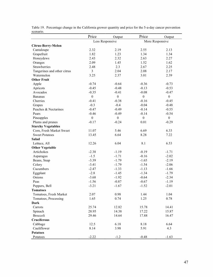
47

Table 19. Percentage change in the California grower quantity and price for the 5-a-day cancer prevention scenario. Price Output Price Output Less Responsive More Responsive Citrus-Berry-Melon Cantaloupe 2.32 2.19 2.55 2.13 Grapefruit 1.82 1.23 1.34 1.34 Honeydews 2.43 2.32 2.63 2.27 Oranges 2.09 1.45 1.52 1.62 Strawberries 2.48 2.3 2.67 2.25 Tangerines and other citrus 3 2.04 2.08 2.17 Watermelon 3.25 2.37 3.01 2.39 Other Fruit Apple -0.74 -0.64 -0.36 -0.73 Apricots -0.45 -0.48 -0.13 -0.53 Avocados -0.35 -0.41 -0.08 -0.47 Bananas 0 0 0 0 Cherries -0.41 -0.38 -0.16 -0.45 Grapes -0.3 -0.4 -0.04 -0.48 Peaches & Nectarines -0.47 -0.49 -0.14 -0.55 Pears -0.46 -0.49 -0.14 -0.54 Pineapples 0 0 0 0 Plums and prunes -0.17 -0.24 0.01 -0.29 Starchy Vegetables Corn, Fresh Market Sweet 11.07 5.46 6.69 6.33 Sweet Potatoes 13.45 6.64 8.28 7.22 Salad Lettuce, All 12.26 6.04 8.1 6.53 Other Vegetable Artichokes -2.38 -1.19 -0.19 -1.71 Asparagus -1.5 -1.71 -0.16 -2.02 Beans, Snap -3.39 -1.79 -1.65 -2.19 Celery -3.41 -1.79 -1.54 -2.06 Cucumbers -2.47 -1.33 -1.13 -1.66 Eggplant -2.8 -1.45 -1.34 -1.79 Onions -3.68 -1.92 -0.64 -2.34 Peas -1.56 -0.87 -0.67 -1.19 Peppers, Bell -3.21 -1.67 -1.52 -2.01 Tomatoes Tomatoes, Fresh Market 2.07 0.98 1.44 1.04 Tomatoes, Processing 1.65 0.74 1.25 0.78 Dark Carrots 25.74 12.82 15.78 14.41 Spinach 28.95 14.38 17.22 15.87 Broccoli 29.46 14.64 17.88 16.47 Cruciferous Cabbage 12.5 6.18 8.18 6.64 Cauliflower 8.14 3.98 5.91 4.3 Potatoes Potatoes -2.22 -1.2 -0.48 -1.63

48

than the change in price. When the supply elasticities are less responsive, most fruits in the “other” fruit category and asparagus have changes in output that are greater than the changes in prices. The fruits within the “other” sub-group that have changes in prices that are greater than the changes in output are apples and cherries. When the supply elasticities are more responsive, the percentage change in output for all crops within the “other” fruit and “other” vegetable sub-groups, and for citrus crops is greater than the change in prices. Farmland is being taken out of production of the crops with falling prices and transferred into the crops with rising prices. For the citrus crops, with a higher supply elasticity than the row vegetable crops, land is more easily transferred into citrus production than in row vegetable production. However, for the row fruit crops comprised of melons and strawberries, when the supply elasticity becomes larger, and supply elasticities are more responsive to price changes, less land is put into production of those crops than when the supple elasticity is less responsive. Instead, growers maximize profits by putting less land into production than when the supply elasticities are less responsive, and increasing prices. 7-a-day When the supply elasticities are less responsive, there is the same pattern in the changes in the grower share of the retail dollar as the 5-a-day scenario (Table 20). Growers are getting a larger share of the retail dollar for all commodities except for strawberries and asparagus. When the supply elasticities are more responsive, there are a few differences. In the 5-a-day scenario growers got a larger share of the retail price for fruit crops and a smaller share for vegetables. Now, growers are getting a smaller share of the retail price for many fruit crops including strawberries, apples, oranges, grapes and cherries. Apples have the lowest elasticity of demand. The initial shift in quantity demanded raises prices for this crop more than for the other crops. Growers adjust not only by producing more, but by producing relatively more apples than of the other crops. However, the higher prices cause consumers to demand less of the product, putting downward pressure on prices. Therefore, the final change in prices and quantity is high, but not the highest among the fruit crops. For oranges the opposite occurs. Oranges have the highest elasticity of demand. Small price changes result in large adjustments in quantity demanded. Conversely, large changes in quantity demanded are needed before prices change. With a relatively large elasticity of demand, the initial shift in quantity demanded raises prices for oranges less than it does for other fruit crops. The relatively lower prices cause growers to adjust by putting less acreage into production for oranges than for other crops, and consumers to demand more, putting upward pressure on prices. The final changes in prices is low, but not the lowest. For both apples and oranges however, the grower is making larger adjustments in production in response to the relatively higher prices for apples and the relatively lower prices for oranges. The share the grower receives of the retail price declines.

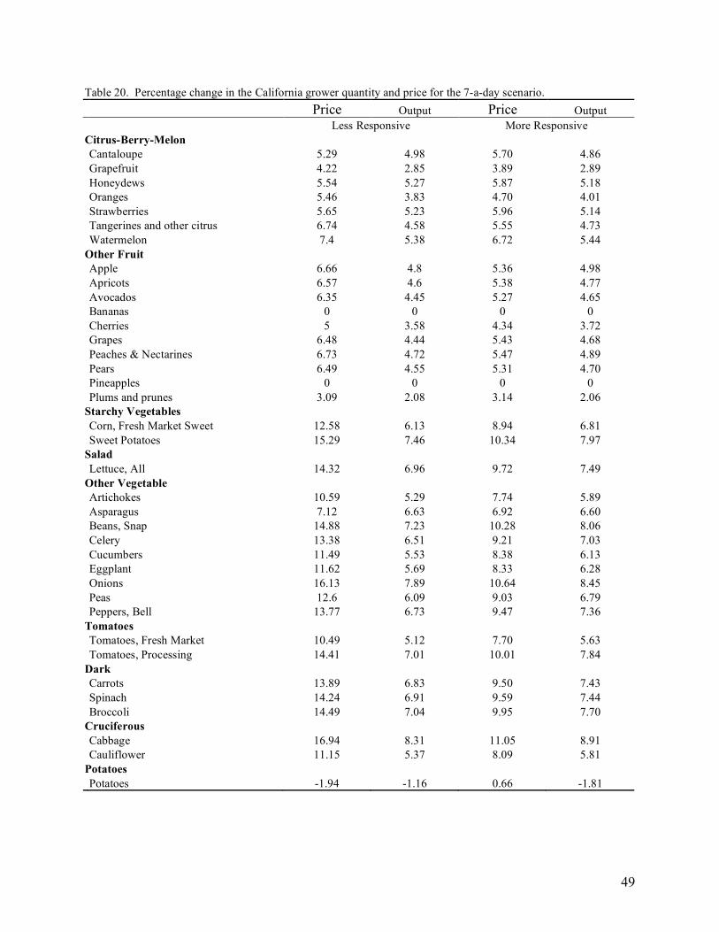
49

Table 20. Percentage change in the California grower quantity and price for the 7-a-day scenario. Price Output Price Output Less Responsive More Responsive Citrus-Berry-Melon Cantaloupe 5.29 4.98 5.70 4.86 Grapefruit 4.22 2.85 3.89 2.89 Honeydews 5.54 5.27 5.87 5.18 Oranges 5.46 3.83 4.70 4.01 Strawberries 5.65 5.23 5.96 5.14 Tangerines and other citrus 6.74 4.58 5.55 4.73 Watermelon 7.4 5.38 6.72 5.44 Other Fruit Apple 6.66 4.8 5.36 4.98 Apricots 6.57 4.6 5.38 4.77 Avocados 6.35 4.45 5.27 4.65 Bananas 0 0 0 0 Cherries 5 3.58 4.34 3.72 Grapes 6.48 4.44 5.43 4.68 Peaches & Nectarines 6.73 4.72 5.47 4.89 Pears 6.49 4.55 5.31 4.70 Pineapples 0 0 0 0 Plums and prunes 3.09 2.08 3.14 2.06 Starchy Vegetables Corn, Fresh Market Sweet 12.58 6.13 8.94 6.81 Sweet Potatoes 15.29 7.46 10.34 7.97 Salad Lettuce, All 14.32 6.96 9.72 7.49 Other Vegetable Artichokes 10.59 5.29 7.74 5.89 Asparagus 7.12 6.63 6.92 6.60 Beans, Snap 14.88 7.23 10.28 8.06 Celery 13.38 6.51 9.21 7.03 Cucumbers 11.49 5.53 8.38 6.13 Eggplant 11.62 5.69 8.33 6.28 Onions 16.13 7.89 10.64 8.45 Peas 12.6 6.09 9.03 6.79 Peppers, Bell 13.77 6.73 9.47 7.36 Tomatoes Tomatoes, Fresh Market 10.49 5.12 7.70 5.63 Tomatoes, Processing 14.41 7.01 10.01 7.84 Dark Carrots 13.89 6.83 9.50 7.43 Spinach 14.24 6.91 9.59 7.44 Broccoli 14.49 7.04 9.95 7.70 Cruciferous Cabbage 16.94 8.31 11.05 8.91 Cauliflower 11.15 5.37 8.09 5.81 Potatoes Potatoes -1.94 -1.16 0.66 -1.81

50

Grape growers also receive a lower share of the retail price when the supply elasticities are more responsive. Grapes are the commodities with the highest cost share for labor. The cost of labor increases with the increase in quantity demanded of fruit and vegetables because fruit and vegetable production uses labor more abundantly than most other commodities in California. With a relatively larger increase in input costs, growers respond by making greater adjustments in production. For cherries it is unclear what is driving grower adjustments compared to the other crops. Cherries receiving a lower share of the retail price would be due to some combination of elasticities of demand and supply, and cost increases. The percentage change in quantity is less than the percentage change in price for all commodities. This holds under both supply elasticity response scenarios. This is a slight change from the 5-a-day scenario. Under the 5-a-day scenario, when the supply elasticities are more responsive, the percentage change in quantity for asparagus was greater than the percentage change in price. 7-a-day cancer prevention Under the 7-a-day cancer prevention scenario, quantity demanded for all commodities increases, with the quantity demanded for the cancer prevention sub-groups shifting up more than for the “other” fruit and the “other” vegetable sub-groups (Table 21). Consequently, the largest price increases are for the cancer prevention commodities. When the supply elasticities are less responsive, growers receive a higher share of the retail dollar for all commodities except oranges, strawberries and asparagus. Oranges have the lowest elasticity of supply, and strawberries and asparagus have a large number of commodities that are substitutes in production. When the supply elasticities are more responsive, growers respond to the greater prices for the cancer prevention subgroups and greater flexibility in planting decisions by adjusting production toward the citrus/berry/melon group, starchy vegetables, salad vegetables, tomatoes, dark and cruciferous vegetables. They receive a lower share of the retail price for the above commodities, Growers received a greater share of the retail price for melons, “other” fruit - except grapes, “other” vegetables, and potatoes. While melons are in the citrus/berry/melon group and production now increases when supply elasticities are more responsive than when they are less, the final adjustments by growers are relatively less given the commodities’ larger own-price elasticity of supply. Because the “other” fruit and “other” vegetable categories have the smallest shift in demand, the price for these commodities increases by a smaller amount than for the remaining commodities. Growers maximize profits by adjusting less into crops in the “other” categories, and, therefore, receive a larger share of the retail dollar.

51

Table 21. Percentage change in the California grower quantity and price for the 7-a-day cancer prevention scenario. Price Output Price Output Less Responsive More Responsive Citrus-Berry-Melon Cantaloupe 7.06 6.74 6.77 6.78 Grapefruit 5.57 3.86 4.7 4.04 Honeydews 7.41 7.13 6.99 7.19 Oranges 6.96 4.95 5.63 5.31 Strawberries 7.52 7.09 7.06 7.16 Tangerines and other citrus 8.98 6.26 6.88 6.53 Watermelon 9.94 7.28 8.16 7.51 Other Fruit Apple 4.95 3.51 4.19 3.59 Apricots 5.14 3.52 4.39 3.61 Avocados 5.06 3.47 4.35 3.59 Bananas 0 0 0 0 Cherries 3.88 2.73 3.53 2.79 Grapes 5.22 3.48 4.52 3.61 Peaches & Nectarines 5.25 3.61 4.46 3.7 Pears 5.06 3.47 4.33 3.55 Pineapples 0 0 0 0 Plums and prunes 2.44 1.58 2.63 1.52 Starchy Vegetables Corn, Fresh Market Sweet 14.72 7.2 9.61 8.19 Sweet Potatoes 17.92 8.77 11.64 9.46 Salad Lettuce, All 16.37 7.99 11.29 8.58 Other Vegetable Artichokes 2.69 1.35 3.54 1.12 Asparagus 1.91 1.41 3.13 1.1 Beans, Snap 3.49 1.53 3.15 1.51 Celery 2.73 1.18 2.73 1.15 Cucumbers 2.68 1.13 2.7 1.06 Eggplant 2.74 1.25 2.65 1.2 Onions 3.72 1.67 4.31 1.52 Peas 4.08 1.82 3.46 1.82 Peppers, Bell 3.23 1.45 2.94 1.43 Tomatoes Tomatoes, Fresh Market 4.14 1.94 3.43 1.98 Tomatoes, Processing 4.17 1.9 3.55 1.97 Dark Carrots 31.91 15.83 20.1 17.7 Spinach 35.6 17.59 21.76 19.33 Broccoli 36.24 17.91 22.59 20.05 Cruciferous Cabbage 17.03 8.35 11.55 8.92 Cauliflower 11.19 5.38 8.53 5.76 Potatoes Potatoes -1.78 -1.08 0.61 -1.68

52

The exception is grapes. Grapes have the largest cost share of labor. Although grapes is in the “other” category, the relatively large increase in input costs due to rising labor costs cause growers to adjust out of grapes at a relatively higher rate than for the remaining commodities. When the supply elasticities are more responsive, percentage change in quantity is always less than the percentage change in price except for melons. At 1.25, melons have the largest own-price elasticity of supply, and also the largest cross-price elasticities of supply with respect to changes in the prices of commodities that are substitutes in production. However, the higher prices now received for melons under the 7-a-day cancer prevention scenario means that growers are less likely to adjust into other crops, and instead put more resources into the production of melons. Growers – Rest of the U.S. Growers in the U.S. are influenced by changes in retail prices in the same way as growers in California. However, the agricultural input markets for the rest of the U.S. were not incorporated into the model due to a lack of available data. Therefore, changes in agricultural input prices are not included, and are not reflected in the planting decisions for growers. Because growers in both regions have the same supply elasticities, the patterns in the percentage changes in prices and production are very close with respect to larger or smaller shares of the retail price, production adjustments and having the percentage change in production always being less than the percentage change in price (Table 22, Table 23, Table 24, Table 25). There is a big difference however in that the price change received by growers in California is always greater than the percentage change in prices for growers in the rest of the U.S. In addition, the percentage change in output for California growers is always less than the percentage change in output for growers in the rest of the U.S. This is because California growers face rising input costs, while the input market is not included in the model for the rest of the U.S. When input costs rise, production decreases and prices go up for the commodity as growers attempt to recoup the higher input costs. While the agricultural input market is missing for growers in the rest of the U.S., its absence illustrates the importance of the input market, and can be used to illustrate the potential effects of regional differences in resource availability and costs. Crops grown in different areas use a different combination of inputs according to the agro-climatic conditions of that area. Therefore, the demand for agricultural inputs, and consequently, the change in prices, will vary by regions. Some regions may experience a greater increase in labor costs, other an increase in water costs, and others a greater increase in land costs. The region facing the greater overall increase in production costs would have a greater increase in grower prices, but a potentially lower increase in profits, than the region having lower price increases. Commodities that use the inputs with the greatest price increases intensively would also experience smaller increases in output than commodities with smaller increases in total input costs.

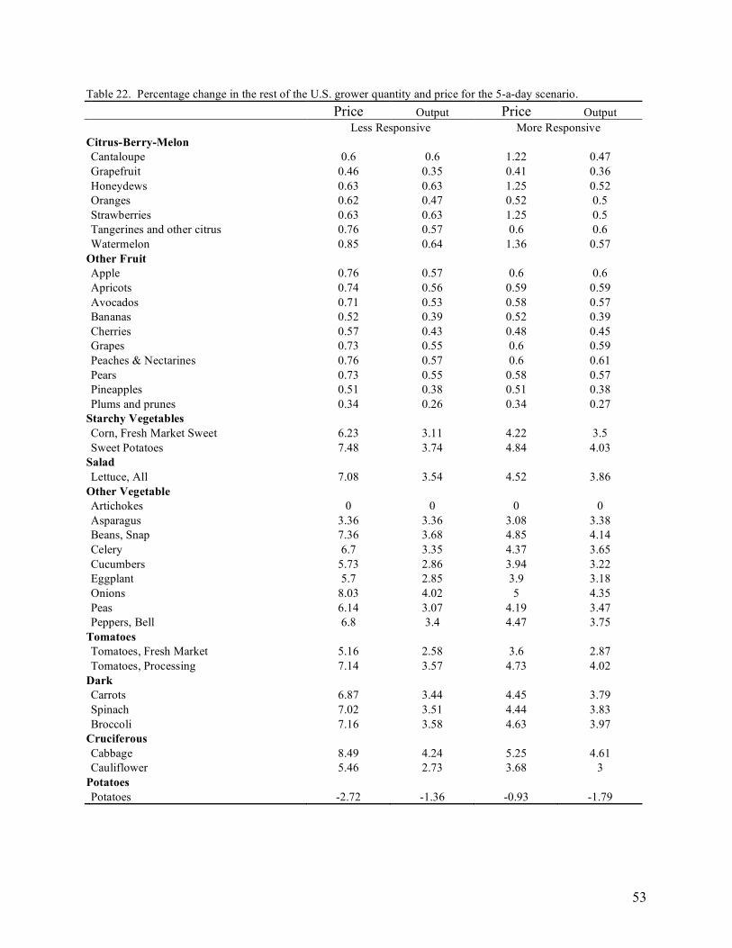
53

Table 22. Percentage change in the rest of the U.S. grower quantity and price for the 5-a-day scenario. Price Output Price Output Less Responsive More Responsive Citrus-Berry-Melon Cantaloupe 0.6 0.6 1.22 0.47 Grapefruit 0.46 0.35 0.41 0.36 Honeydews 0.63 0.63 1.25 0.52 Oranges 0.62 0.47 0.52 0.5 Strawberries 0.63 0.63 1.25 0.5 Tangerines and other citrus 0.76 0.57 0.6 0.6 Watermelon 0.85 0.64 1.36 0.57 Other Fruit Apple 0.76 0.57 0.6 0.6 Apricots 0.74 0.56 0.59 0.59 Avocados 0.71 0.53 0.58 0.57 Bananas 0.52 0.39 0.52 0.39 Cherries 0.57 0.43 0.48 0.45 Grapes 0.73 0.55 0.6 0.59 Peaches & Nectarines 0.76 0.57 0.6 0.61 Pears 0.73 0.55 0.58 0.57 Pineapples 0.51 0.38 0.51 0.38 Plums and prunes 0.34 0.26 0.34 0.27 Starchy Vegetables Corn, Fresh Market Sweet 6.23 3.11 4.22 3.5 Sweet Potatoes 7.48 3.74 4.84 4.03 Salad Lettuce, All 7.08 3.54 4.52 3.86 Other Vegetable Artichokes 0 0 0 0 Asparagus 3.36 3.36 3.08 3.38 Beans, Snap 7.36 3.68 4.85 4.14 Celery 6.7 3.35 4.37 3.65 Cucumbers 5.73 2.86 3.94 3.22 Eggplant 5.7 2.85 3.9 3.18 Onions 8.03 4.02 5 4.35 Peas 6.14 3.07 4.19 3.47 Peppers, Bell 6.8 3.4 4.47 3.75 Tomatoes Tomatoes, Fresh Market 5.16 2.58 3.6 2.87 Tomatoes, Processing 7.14 3.57 4.73 4.02 Dark Carrots 6.87 3.44 4.45 3.79 Spinach 7.02 3.51 4.44 3.83 Broccoli 7.16 3.58 4.63 3.97 Cruciferous Cabbage 8.49 4.24 5.25 4.61 Cauliflower 5.46 2.73 3.68 3 Potatoes Potatoes -2.72 -1.36 -0.93 -1.79

54

Table 23. Percentage change in the rest of the U.S. grower quantity and price for the 5-a-day cancer prevention scenario. Price Output Price Output Less Responsive More Responsive Citrus-Berry-Melon Cantaloupe 2.22 2.22 2.41 2.18 Grapefruit 1.71 1.28 1.16 1.42 Honeydews 2.35 2.35 2.5 2.32 Oranges 1.99 1.5 1.37 1.7 Strawberries 2.3 2.3 2.45 2.27 Tangerines and other citrus 2.8 2.1 1.8 2.25 Watermelon 3.19 2.39 2.9 2.43 Other Fruit Apple -0.82 -0.62 -0.49 -0.68 Apricots -0.58 -0.44 -0.33 -0.47 Avocados -0.49 -0.37 -0.28 -0.41 Bananas -0.38 -0.28 -0.38 -0.29 Cherries -0.47 -0.36 -0.27 -0.4 Grapes -0.44 -0.33 -0.26 -0.38 Peaches & Nectarines -0.6 -0.45 -0.34 -0.49 Pears -0.6 -0.45 -0.34 -0.48 Pineapples -0.41 -0.31 -0.42 -0.31 Plums and prunes -0.27 -0.2 -0.14 -0.23 Starchy Vegetables Corn, Fresh Market Sweet 10.99 5.49 6.55 6.38 Sweet Potatoes 13.34 6.67 8.11 7.27 Salad Lettuce, All 12.15 6.08 7.93 6.58 Other Vegetable Artichokes 0 0 0 0 Asparagus -1.66 -1.66 -0.38 -1.96 Beans, Snap -3.5 -1.75 -1.84 -2.14 Celery -3.51 -1.75 -1.71 -2.01 Cucumbers -2.58 -1.29 -1.31 -1.6 Eggplant -2.86 -1.43 -1.46 -1.75 Onions -3.78 -1.89 -0.8 -2.29 Peas -1.67 -0.83 -0.84 -1.13 Peppers, Bell -3.29 -1.65 -1.66 -1.96 Tomatoes Tomatoes, Fresh Market 2.01 1 1.33 1.07 Tomatoes, Processing 1.54 0.77 1.08 0.82 Dark Carrots 25.68 12.84 15.67 14.45 Spinach 28.83 14.41 17.04 15.92 Broccoli 29.35 14.68 17.71 16.53 Cruciferous Cabbage 12.42 6.21 8.04 6.69 Cauliflower 8.03 4.02 5.74 4.36 Potatoes Potatoes -2.33 -1.16 -0.65 -1.58

55

Table 24. Percentage change in the rest of the U.S. grower quantity and price for the 7-a-day scenario. Price Output Price Output Less Responsive More Responsive Citrus-Berry-Melon Cantaloupe 5.06 5.06 5.29 5.01 Grapefruit 3.96 2.97 3.49 3.06 Honeydews 5.34 5.34 5.49 5.32 Oranges 5.26 3.94 4.37 4.19 Strawberries 5.23 5.23 5.39 5.23 Tangerines and other citrus 6.3 4.72 4.95 4.92 Watermelon 7.24 5.43 6.39 5.56 Other Fruit Apple 6.48 4.86 5.07 5.08 Apricots 6.26 4.7 4.94 4.91 Avocados 6.05 4.54 4.84 4.79 Bananas 4.42 3.31 4.38 3.28 Cherries 4.85 3.64 4.08 3.82 Grapes 6.14 4.6 4.94 4.91 Peaches & Nectarines 6.42 4.81 5.03 5.03 Pears 6.18 4.64 4.87 4.82 Pineapples 4.32 3.24 4.3 3.23 Plums and prunes 2.88 2.16 2.81 2.19 Starchy Vegetables Corn, Fresh Market Sweet 12.4 6.2 8.63 6.93 Sweet Potatoes 15.05 7.53 9.9 8.1 Salad Lettuce, All 14.07 7.04 9.23 7.64 Other Vegetable Artichokes 0 0 0 0 Asparagus 6.74 6.74 6.35 6.77 Beans, Snap 14.61 7.3 9.85 8.18 Celery 13.16 6.58 8.84 7.15 Cucumbers 11.23 5.61 7.97 6.26 Eggplant 11.47 5.74 8.06 6.36 Onions 15.9 7.95 10.16 8.59 Peas 12.36 6.18 8.63 6.94 Peppers, Bell 13.57 6.79 9.15 7.46 Tomatoes Tomatoes, Fresh Market 10.34 5.17 7.43 5.72 Tomatoes, Processing 14.16 7.08 9.62 7.94 Dark Carrots 13.75 6.87 9.14 7.55 Spinach 13.97 6.99 9.07 7.59 Broccoli 14.25 7.12 9.46 7.87 Cruciferous Cabbage 16.75 8.37 10.62 9.06 Cauliflower 10.91 5.46 7.59 5.98 Potatoes Potatoes -2.17 -1.09 0.22 -1.67

56

Table 25. Percentage change in the rest of the U.S. grower quantity & price for the 7-a-day cancer prevention scenario. Price Output Price Output Less Responsive More Responsive Citrus-Berry-Melon Cantaloupe 6.83 6.83 6.39 6.92 Grapefruit 5.31 3.98 4.3 4.22 Honeydews 7.21 7.21 6.65 7.31 Oranges 6.75 5.07 5.3 5.49 Strawberries 7.03 7.03 6.49 7.19 Tangerines and other citrus 8.53 6.4 6.26 6.73 Watermelon 9.78 7.34 7.86 7.62 Other Fruit Apple 4.77 3.58 3.89 3.7 Apricots 4.83 3.62 3.94 3.76 Avocados 4.76 3.57 3.92 3.73 Bananas 3.45 2.58 3.4 2.55 Cherries 3.73 2.79 3.27 2.89 Grapes 4.87 3.65 4.01 3.85 Peaches & Nectarines 4.94 3.71 4.01 3.84 Pears 4.75 3.56 3.88 3.68 Pineapples 3.32 2.49 3.3 2.48 Plums and prunes 2.22 1.67 2.29 1.65 Starchy Vegetables Corn, Fresh Market Sweet 14.54 7.27 9.3 8.31 Sweet Potatoes 17.68 8.84 11.23 9.58 Salad Lettuce, All 16.12 8.06 10.85 8.71 Other Vegetable Artichokes 0 0 0 0 Asparagus 1.52 1.52 2.58 1.26 Beans, Snap 3.21 1.61 2.72 1.63 Celery 2.5 1.25 2.36 1.27 Cucumbers 2.42 1.21 2.28 1.19 Eggplant 2.59 1.29 2.37 1.28 Onions 3.48 1.74 3.89 1.64 Peas 3.83 1.91 3.06 1.97 Peppers, Bell 3.03 1.51 2.62 1.53 Tomatoes Tomatoes, Fresh Market 3.98 1.99 3.15 2.07 Tomatoes, Processing 3.92 1.96 3.15 2.07 Dark Carrots 31.76 15.88 19.79 17.8 Spinach 35.33 17.67 21.3 19.47 Broccoli 35.99 17.99 22.15 20.2 Cruciferous Cabbage 16.84 8.42 11.18 9.05 Cauliflower 10.94 5.47 8.09 5.91 Potatoes Potatoes -2.02 -1.01 0.21 -1.55

57

Input usage in California Because prices and production do not change very much in response to greater demand by Californians, the price of land and labor does not change very much, especially for the 5-a-day and 5-a-day cancer prevention scenarios (Table 26). When supply elasticities are less responsive, for the 5-a-day scenario the increase in the price of land is 0.90 percent and for labor is it 0.16 percent. For the 5-a-day cancer prevention scenario the increase in the price of land goes up to 1.18 percent and the price of labor by 0.22 percent. The increase almost doubles under the 7-a-day scenarios. The price of land increases by 2.59 percent and for labor it increases by 0.52 percent. For the 7-a-day cancer prevention scenario the increase in the price of land is slightly less at 2.57 percent and for labor it is only 0.54 percent. There is no increase in the price of water because water is not priced through market transactions in California.

Table 26. Percentage change in agricultural inputs Less Responsive 5-a-day 5-a-day cp 7-a-day 7-a-day cp Price Land 0.90 1.18 2.59 2.57 Price Labor 0.16 0.22 0.52 0.54 Quantity land 1.80 2.36 5.18 5.14 Quantity labor 1.61 2.20 5.20 5.43 Quantity Water 1.32 1.63 4.84 4.78 More Responsive 5-a-day 5-a-day cp 7-a-day 7-a-day cp Price Land 0.97 1.29 2.76 2.75 Price Labor 0.17 0.24 0.55 0.57 Quantity land 1.95 2.57 5.53 5.49 Quantity labor 1.71 2.36 5.47 5.75 Quantity Water 1.42 1.79 5.14 5.09

Because the agricultural inputs used can be substituted for one another to some extent in production the percentage change in the use of the agricultural inputs is not equal. For the 5-a-day scenario the quantity of land used increases by 1.80 percent, labor increases by 1.61 percent and water by 1.32 percent. For the 7-a-day scenario land increases by 5.18 percent, labor by 5.20 percent and water by 4.84 percent. When supply elasticities are more responsive the price and quantity demanded for agricultural inputs increases. As stated previously, as the elasticity of becomes more responsive, the percentage change in production increases. This causes the use of agricultural inputs to increase, causing their price to increase. Therefore, when the supply responsive is more elastic, the increases in input prices are 0.97 for land, and 0.17 for labor. Prices increase slightly for the 5-a-day cancer prevention scenario, but increase much more for the 7-a-day scenario. The price increases under the 7-a-day scenario are 2.76 percent for land and 0.55 percent for labor. The

58

change in the price of land decreased slightly to 2.75 percent for the 7-a-day cancer prevention scenario, but increases to 0.57 percent for labor. Costs and Benefits to Consumers and Producers Consumers are affected by the change in retail prices, the change in quantity consumed, and, for Californians, the change in quantity demanded for fruits and vegetables. Recall that in this study consumer benefits are estimated as the change in consumer surplus. This is the measurement of the difference between the extra amount people are willing to spend to eat healthier, and the actual amount they do spend. The societal benefits from a lower incidence of cancer are not included in this analysis. Growers are affected by the change in grower prices and production. Grower benefits are estimated as the change in producer surplus. This is the measurement of the difference between the economic costs of producing a commodity, and the price received for that commodity. The change in total surplus is then the sum of the change in consumer and producer surplus. 5-a-day Consumers and growers in California both benefit (Table 27). The gains to both low and high-income consumers are about the same under both supply response scenarios. The annual benefits are $2 billion for low-income consumers and $11.9 billion for high income. The benefits are about the same because the benefits are from the increase in quantity demanded for fruits and vegetables. The higher food prices reduce consumer surplus. While about the same, for the citrus/berry/melon subgroup, the benefits when supply elasticities are less responsive are greater than when they are more responsive. This is because of the increase in prices for melons and strawberries as supply becomes more responsive. For all other subgroups, the increase in surplus is less when supply elasticities are more responsive. The share of consumer benefits allocated to each household income group varies in proportion to the share consumed by each group. Low-income households consume more apples, bananas, cabbage, celery, cucumbers, pears, tangerines, and watermelon. Correspondingly, the food sub-groups that contain these items have a larger share of benefits realized by people in low-income households. In the survey of California consumers, no consumption of sweet potatoes was done, and low-income consumers have the smallest share of total consumer surplus for that group. The shares are the same whether the supply response is less or more elastic. There is greater variation in the benefits to growers as the supply elasticities go from less to more responsive. The annual increase in producer surplus for California growers is $316 million when supply elasticities are less responsive and $223 million when supply elasticities are more responsive (Table 27). Grower benefits are lower when supply elasticities become more responsive due to the smaller price increase. In addition, grower benefits are less for all commodity sub-groups except the citrus/berry/melon group. The change in surplus for growers in California increases for the citrus/berry/melon group from eight million a year to 13 million when supply elasticities are more responsive. Producer surplus increases for the citrus/berry/melon groups because prices increase. The loss in producer surplus for potatoes is less when supply elasticities are more responsive. The lower gains to most sub-groups is greater

59

than the gains to the citrus/berry/melon group and lower losses to potatoes, therefore, producer surplus declines as supply elasticities are more responsive. Overall, the greatest gains to California growers are from the salad, dark, tomato, and “other” vegetable sub-group categories due to the relatively large increase in quantity demanded compared to the fruit categories (Table 27). Because producer surplus changes more that consumer surplus as the supply response become more elastic, the change in total surplus is less. The change in surplus goes from $14,296 million when supply elasticities are less responsive to $14,226 million when it is more. Because consumers in the rest of the U.S. are only affected by the changes in prices and quantities, the increase in prices and decrease in consumption leave consumers outside of California worse off. When supply elasticities are less responsive, the decline in consumer surplus for people in the rest of the U.S. is $233 million for low-income households and $2,123 million for high income households (Table 27). Because a larger share of people live in the higher income households, their loss is greater. When supply elasticities are more responsive, people are still worse off, but less so. The decline is now only $221 million for low-income consumers and $2,013 million for high-income consumers. Again, for commodities that low-income consumers eat in greater amounts than high-income consumers, the share of losses incurred by low-income consumers rises. Even though there are more people in the rest of the U.S., the benefits to Californians are greater than the losses to consumers in the rest of the U.S., and the net change in consumer surplus for the U.S. as a whole is positive. While the increase in consumer surplus is less for California when supply elasticities are more responsive, the smaller decrease in consumer surplus for people in the rest of the U.S. makes consumer surplus for the entire U.S. increase as supply becomes more responsive. The annual gain to growers in the rest of the U.S. is $144 million when supply elasticities are less responsive and $166 million when they are more responsive (Table 27). Growers in the rest of the U.S. gain when supply becomes more responsive because the losses to potato growers decline from $199 million a year to $68 million a year. Therefore, even though the change in producer surplus is also not as large for most commodity sub-groups, the lower losses to potato growers outweigh the lower gains in other sub-groups, and the change in producer surplus increases. Even though growers in the rest of the U.S. gain when supply elasticities are more responsive, the lower gains to California producers are greater and the net gain in producer surplus for the entire U.S. declines from $460 million a year when supply elasticities are less responsive to $388 million a year when they are more responsive. The total annual change in surplus to all groups in both regions is $12,080 million when supply elasticities are less responsive and $12,157 when supply elasticities are more responsive. Even though the net gain in producer surplus is lower when supply elasticities are more responsive, the net gain to total surplus is higher due to the higher gains to consumers.

60

5-a-day cancer prevention Because demand falls for the “other” fruit, “other” vegetable, and potato sub-groups, consumer surplus in California falls for those sub-groups, and rises for people in the rest of the U.S. California consumers are worse off because of the fall in demand, while lower prices make consumers in the rest of the U.S. better off (Table 28). In California, the annual increase in consumer surplus is $2,258 million for low-income consumers and $13,978 million for high-income consumers when supply elasticities are less responsive, and $2,264 million for low-income consumer and $14,027 million for high-income consumers when supply elasticities are more responsive. For consumers in the rest of the U.S., the increase in prices for most commodities is large enough to make the total change in consumer surplus negative. When supply elasticities are less responsive the decline in consumer surplus is $161 million for low-income consumers and $1,615 million for high. When supply elasticities are more responsive the decline is $148 for low-income consumers and $1,490 for high (Table 28). The losses to consumers decrease when the supply elasticities become more responsive because the smaller changes in prices leads to both smaller losses in the cancer prevention sub-groups and smaller gains in the remaining groups. However, the smaller losses in the cancer prevention sub-groups outweigh the smaller gains in the remaining groups. There is a net gain in consumer surplus when all people are considered because the gains to California consumers are greater than losses to consumers in the rest of the U.S. When supply elasticities are less responsive, the gain is $2,096 million annually for low-income consumers and $12,367 million for high-income (Table 28). When supply elasticities are more responsive, the gain is $2,114 million for low-income consumers and $12,539 million for high. The larger gains in surplus when supply elasticities are more responsive are due to the lower increase in prices and greater output than when supply elasticities are less responsive. Again, low-income consumers have a higher share of total consumer surplus for sub-groups that contain commodities that low-income consumers eat in greater proportion compared to high-income consumers. In California, the increase in producer surplus is $464 million when supply elasticities are less responsive and $318 million when supply is more (Table 28). Surplus declines when supply elasticities are more responsive because the smaller gains in the cancer prevention sub-groups are greater than the smaller losses by category. The biggest gains are in the dark and salad categories. In these categories, California produces most of the crop marketed in the U.S. California growers have losses for the “other” fruit, “other” vegetable, and potato category due to falling prices. In the rest of the U.S. the increase in producer surplus is $152 million when supply elasticities are less responsive and $176 when they are more responsive (Table 28). Surplus increases for growers in the rest of the U.S. when supply elasticities are more responsive because the smaller losses are greater than the smaller gains in the cancer prevention sub-groups. The largest gains to producers in the rest of the U.S. are with dark and starchy vegetables.

61

For the entire U.S., the gains to producers are $619 million when supply elasticities are less responsive and $494 million when they are more responsive. Surplus goes down when supply elasticities are more responsive because the lower surplus gains to California producers are greater than the higher surplus gains to growers in the rest of the U.S. In California, consumer and producer surplus move in the same direction. Both groups have an increase in surplus for the same commodities and a decrease in the same commodities. The total gains in surplus in California are $16,703 million when supply elasticities are less responsive and $16,608 million when supply elasticities are more responsive. For the rest of the U.S. however, consumer and producer surplus move in the opposite direction. When prices rise, producers are better off while consumers are worse off. The total losses to consumers are greater than the gains to producers, and the net change in surplus follows the direction of change for consumers. Overall, the decline in surplus for both consumers and producers in the rest of the U.S. is $1,624 million when supply elasticities are less responsive and $1,461 when supply elasticities are more responsive. The net losses are lower when supply elasticities are more responsive because the smaller gains are less than the reduction is losses. For the entire U.S., the benefits to both groups in California are greater than the net losses in the rest of the U.S., and the U.S. as a whole benefits (Table 28). The net benefits are $15,080 when supply elasticities are less responsive and $15,147 when supply elasticities are more responsive. Even though the net benefits largely reflect the large gains to consumers in California, it is the increase in surplus to growers in the rest of the U.S. that is sufficient to increase the net surplus for the entire U.S. when supply elasticities are more responsive. 7-a-day The results for the 7-a-day scenario are again very similar to the results for the 5-a-day scenario, except that the magnitudes are greater (Table 29). When supply elasticities are less responsive, the gains to low-income consumers in California are $5,858 million, high-income consumers gain $43,043, growers gain $788 and total gains are $49,687. When supply elasticities are more responsive low-income consumers gain $5,864 million a year, high-income consumers gain $43,099 million, growers gain $583 million, and the total change in surplus is $49,546 million a year. For the rest of the U.S., when supply elasticities are less responsive surplus falls by $674 million for low-income consumers, and by $5,952 million for high-income consumers. When supply elasticities are more responsive surplus falls by only $644 for low-income consumers and $5,688 for high-income consumers. The main difference between the 5-a-day and the 7-a-day scenario is that growers in the rest of the U.S. now have smaller gains when the supply response is more elastic, even though potato growers go from have a loss of $159 million when supply elasticities are less responsive to a gain of $16 million when they are more responsive (Table 29). Total producer surplus is less because the gains in all other sub-categories are less.

62

When supply elasticities are more responsive, the annual net benefits for the U.S. are $$43,773 million when supply elasticities are less responsive and $43,851 million when supply elasticities are more responsive (Table 29). Because producer surplus declines for growers in both California and the rest of the U.S., total producer surplus is now also lower when supply elasticities are more responsive than when they are less responsive. 7-a-day cancer prevention Under the 5-a-day cancer prevention scenario, the consumption of some fruits and vegetables fell in order to increase consumption in the targeted cancer prevention sub-groups. For the 7-a-day cancer prevention scenario however, the consumption of all fruits and vegetables, except potatoes, increases. The gains to consumers in California are $4,785 for low-income households, $35,131 for high-income households and $836 million for growers when supply elasticities are less responsive (Table 30). When supply elasticities are more responsive the annual increase in producer surplus is $4,793 million for low-income households, $35,203 million for high-income households and $613 million for growers. Producer surplus increases in the 7-a-day cancer prevention scenario compared to the 7-a-day general recommendations because California has a large share of production of the cancer prevention commodities (Table 30). For example, when supply elasticities are less responsive and under the general 7-a-day recommendation, producer surplus is $133 million a year for the dark sub-group, and $183 million a year for salad. For the 7-a-day cancer prevention scenario, producer surplus is $336 million for the dark sub-group and $211 for salad. For the rest of the U.S., when supply elasticities are less responsive the losses to consumers are $674 million a year for low-income households, $5,952 million a year for high income households, and the gains to growers are $788 million a year (Table 30). When supply elasticities are more responsive, the losses in consumer surplus are $494 million for low-income households, $4,474 million for high income households, and the gains to growers are $562 a year. As is the case with California growers, the gain to growers in the rest of the U.S. are now lower when supply elasticities are more responsive than when supply elasticities are less responsive. Even though the gains to growers are less when supply elasticities are more responsive, total surplus for when all groups in all regions is greater. This is because the additional gains to consumer surplus are greater than the smaller gains to growers.