The direct economic effects of a policy to provide government subsidized price discounts

for the purchase of fruit and vegetable by food stamp recipients.

by

Karen M. Jetter Assistant Research Economist

Agricultural Issues Center 1 Shields Ave.

University of California Davis, CA 95616

telephone: 530-754-8756 e-mail: jetter@primal.ucdavis.edu

1

INTRODUCTION

This study will evaluate the direct benefits and costs to consumers and producers from

changes in prices, consumption and production, of a policy to offer government price discounts

on fresh fruit and vegetable to food stamp recipients. The suggestion for a price discount on fruit

and vegetable for food stamps recipients is contained in the 2004 Farm Bill, section 4116 that

provides for research on “encouraging consumption of fruit and vegetables by developing a cost-

effective system for providing discounts for purchases of fruit and vegetables made through use

of electronic benefit transfer (EBT) cards”. In California, legislation has been proposed (AB

2384) to complete a pilot study of providing a price discount of 20% to 40% to food stamp

recipients for every dollar spent on fruit and vegetable purchases. To date no studies have been

completed to determine if, or under what circumstances, this is an economically viable option.

The price discount for the purchase of fruit and vegetables would take place at the cash

register when food stamp users swipe their EBT cards. The technology to provide the discount is

the same as the technology used by supermarkets that offer discounts to shoppers who use their

in-store “club” card and is administratively feasible (personal communication, Don Harris, Vice

President, Produce Department, Safeway, Inc., 1999). The question remains whether it is

economically feasible.

Increased consumption of fruit and vegetable has been linked to a decrease in dietary

related chronic diseases such as heart disease, diabetes and some cancers (Hung et al., 2004).

Low socioeconomic status (SES) is strongly associated with higher rates of obesity and high

rates of the leading causes of illness and death. For instance, results from the National Health

Interview Survey show that low SES adults are more likely to have diabetes, cancer, heart

disease, and hypertension compared to those with higher SES (Mokdad et al. 2001; Paeratakul et

2

al. 2002). They are also more likely to be diagnosed in the later stages of chronic diseases such

as cancer and, consequently, have higher mortality rates than their higher income counterparts

(Bradley et al. 2005). Diet may play an important mediating role in explaining socioeconomic

disparities in health status. Analyses of data from the Continuing Survey of Food Intakes of

Individuals (CSFII) indicate that wealthier respondents eat more fruit and vegetable, and eat a

greater variety of foods, than their lower-income counterparts (Haan et al. 2001).

About half of all food stamp recipients are persistently on food stamps. Even though

70% of all recipients leave within two years, more than half of those who leave the program will

return within two years (Gleason et al. 1998). Consequently, developing cost effective policies

that lead to a higher consumption of fruit and vegetable may have a significant impact on the

incidence of chronic disease among persistent food stamp recipients.

Improving diet quality by eating according to the newly revised food pyramid guidelines

(www.mypyramid.com) may strain low-income household budgets. Current recommendations

for healthy eating include eating whole grain products and very lean meat. However, the

additional cost eating whole grains and lower fat meat is about 17% more than the level of food

stamp benefits based on the Thrifty Food Plan (Jetter and Cassady 2006) as the Thrifty Food

Plan does not include whole grains or very lean ground beef (USDA 1999). The availability of

healthier foods may also be a problem. To economize low-income consumers often buy bulk

items that have a lower per unit cost (Kaufman et al. 1997). When it comes to the purchase of

healthier foods however this may not be a feasible strategy as whole grains, very lean meat and

skinless poultry are rarely sold in the large “family” packs in which white flour or rice, white

breads, and higher fat ground meat and poultry are often sold (Jetter and Cassady 2006).

3

Therefore, a policy that eases budgetary constraints of low-income consumers may promote

healthier eating habits among that group.

To assist food stamp recipients in meeting the revised guidelines, a general increase in

assistance can be provided, or a policy that targets the healthier food items can be adopted. With

respect to general assistance, Blisard et al. (2004) estimated that an additional dollar of income in

a low-income household (less than 130 percent of the poverty line) will probably be allocated to

food groups other than fruit and vegetable, or to other items that are deemed more important by

the household. Conversely, in a review of environmental interventions, Seymour et al (2004)

determined that targeted assistance may be more efficient at effectuating dietary changes than

more general assistance programs. As reported in the review, interventions that offered

discounts of 25% to 50% resulted in a significant change in consumption to healthier foods.

Price discounts of 10% did not have a significant effect. In a study on the effect of labeling and

price discounts on snack items in vending machines French et al. (2001) estimated that price

discounts of 25% and 50% lead to an increase in the purchase of healthier snacks by 39% and

93% respectively. Labeling alone or in combination with price discounts did not have a

significant effect.

The potential to improve the health status of food stamp consumers is the impetus behind

a government subsidized price discount policy. Providing price discounts also directly benefits

food stamp consumers through lowering the prices that they pay for fruit and vegetables.

However, a price discount may cause equilibrium market prices to rise for fruit and vegetables as

the discount would cause the quantity demanded of fruit and vegetables to increase. This would

benefit growers of fruit and vegetable as they are now receiving higher prices for their products,

but make non-food stamp consumers potentially worse off. Tax payers would also bear the

4

burden of paying stores for the difference between market prices and the price discounts.

Including these effects on all groups is essential when calculating the total costs and benefits of a

policy change.

Graphical analysis of the costs and benefits to consumers and producers of a food stamp

bonus value coupon.

The graphical analysis of the market for a commodity is for the case of a large country and is

either a net importer or a net exporter of a commodity. The case of a net importer is presented

first, then the case of the net exporter will be presented.

If the U.S. domestic market is a net importer of a commodity, insufficient quantity is

produced within the country, so the country has an excess demand for the commodity that is

satisfied by imports. The initial equilibrium price is Po. At the market price of Po the initial

quantity demanded by food stamp recipients is dofs, the quantity demanded by other consumers is

doo, and total quantity demanded is doall.

5

The bonus value coupon causes the quantity demanded to increase to d1fs. The greater demand

from commodity i causes an increase in the market price to P1. At P1 quantity demanded by

other consumers falls to d1o but quantity demanded by both food stamp and non food stamp

recipients increases to d1all.

Given the relatively small share of food stamp users in the general population (only four

percent of respondents in the NHANES 2001-2002 & 2003-2004 surveys), the change in market

price is anticipated to be minimal, causing minimal changes in consumption by non-food stamp

consumers, and only a slight increase in output by growers. However, given the size of the U.S.

agricultural sector, even a slight change in output may have large benefits to growers. For

example, increasing the consumption of fruit and vegetable by Californians from about 4

servings a day to 5 a day benefits all growers in the U.S. by approximately $460 million a year

(Jetter et al 2004).

Food stamp recipients stand to benefit substantially depending on the level of price

discount and their responsiveness to price changes. An additional indirect benefit would be a

6

reduction in chronic diseases, such as cancer, among the low-income population that is the focus

of the price discount policy. The benefits may include both a reduction in mortality and a

reduction in public expenditures such as Medicaid. While very important benefits, undertaking

an epidemiology study of the potential change in incidence of chronic diseases in beyond the

scope of this small grant proposal.

Hypotheses to be evaluated

1. Offering price discounts of 25% or 40% to food stamp recipients for the purchase of fruit

and vegetables will substantially increase consumption of fruits and vegetables.

2. Even though non-food stamp recipients may be worse off, the total direct benefits to

consumers and producers would provide economic justification for a policy of price

discounts to food stamp recipients for fruits and vegetables.

METHODOLOGY

Data analysis strategy.

The analysis involves using a model of the U.S. fruit and vegetable industry that captures

the effects of price discounts on market prices and supply, quantity demanded, trade and

production. The model is solved for the new equilibrium price and quantity for a given price

discount. The basic model sets out supply and demand conditions in log-differential form such

that dlnX = (X1 – X0)/X0 , where the subscript 1 indexes the new price or quantity level and the

subscript 0 indexes the original level of variable X. The model is used to show how the

equilibrium quantities, prices and other variables respond to shocks to the system, such as a price

discount. The supply side of the model contains equations for net U.S. trade (U.S. imports minus

U.S. exports), market quantity supplied from the agricultural marketing sector (processors and

handlers), and production supplied to the marketing sector from growers in California and the

7

rest of the U.S. The result is a model that links supply and demand in the final market to supply

and demand in the marketing sector, and ultimately, to growers’ production decisions. The

solution to the system of equations is the percentage change in retail and grower prices, final

quantity demanded by each consumer group in the study, imports and exports, and production by

growers in each region.

The advantage of simulating a linear market model is that it does not require estimating

the underlying supply and demand curves. The supply and demand functions are log-linear

approximations to the underlying curves. For small changes in demand they provide estimates of

surplus changes that are a close approximation to the actual values (Alston, Norton, and Pardey

1995). Another advantage is that the system can be simulated with readily available information

(Alston, Norton, and Pardey 1995). The main disadvantage is that the larger the shock to the

system, the more biased is the estimate of surplus changes. However, this is true for any model

where the demand curve is an approximation.

Similar market models have been widely used to estimate the benefits of agricultural

research (e.g., Alston, Norton, and Pardey 1995), agricultural policies (e.g., Sumner and Lee

1997) and changes in consumption following nutrition education to school age children (Alston,

Chalfant, and James 1999). They do not predict what the actual market quantity and prices will

be, because many other factors influence actual production (such as temperature, rainfall, etc.),

market price, and market quantity each year. Instead, this model allows the economic effects of

increased consumption to be modeled separately from all other market influences, treating the

other market conditions and production costs as remaining constant when the change occurs.

This is, in fact, the preferred measure of the effects of an isolated incident, even if interest is in a

real-world demand shift, not a hypothetical one. Simply looking at the market before and after

8

the change, and attributing the entire change to the demand shift, runs the risk of interpreting the

effects of weather or other changes on production as the effects of the demand shift alone.

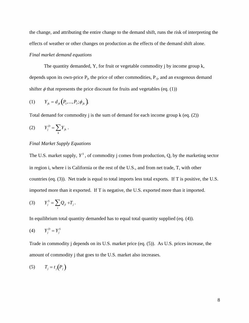
Final market demand equations

The quantity demanded, Y, for fruit or vegetable commodity j by income group k,

depends upon its own-price Pj, the price of other commodities, P-j, and an exogenous demand

shifter φ that represents the price discount for fruits and vegetables (eq. (1))

(1) Yjk = djk P1,...,PJ ;φ jk( ).

Total demand for commodity j is the sum of demand for each income group k (eq. (2))

(2) YjD = Yjk

k∑ .

Final Market Supply Equations

The U.S. market supply, Y S , of commodity j comes from production, Q, by the marketing sector

in region i, where i is California or the rest of the U.S., and from net trade, T, with other

countries (eq. (3)). Net trade is equal to total imports less total exports. If T is positive, the U.S.

imported more than it exported. If T is negative, the U.S. exported more than it imported.

(3) YjS = Qji +

i∑ Tj .

In equilibrium total quantity demanded has to equal total quantity supplied (eq. (4)).

(4) YjD = Yj

S

Trade in commodity j depends on its U.S. market price (eq. (5)). As U.S. prices increase, the

amount of commodity j that goes to the U.S. market also increases.

(5) Tj = t j Pj( )

9

Marketing Sector

The marketing sector takes the farm product and either packs it fresh for delivery to markets, or

processes it to sell as juiced, canned, frozen or dried products. Non-farm inputs such as labor,

transportation, packing materials, machinery in processing plants, etc., are used to bring fresh

and processed fruits and vegetables to market. The total cost of the non-farm inputs is wm . The

price received by growers of fruits and vegetables, wg , will change as the quantity demanded for

fruits and vegetables changes in response to the price discount for food stamp recipients. The

retail price depends upon the cost of the farm and non-farm inputs in each region i (eq. (6)).

(6) Pj = Cji wjgi ,wjmi( )

The marketing sector receives the farm commodity from growers and the non-farm inputs from

other suppliers. As demand for the final output changes, demand for the farm commodity and

non-farm inputs changes. Using Shepard’s Lemma, the derived demand for the farm

commodity, x jgi, (eq. (7)) by the marketing sector in each region is

(7) xjgi = ∂Cji wjgi ,wjm;Qji( )/ ∂wjgi .

Again using Shepard’s Lemma, the derived demand for the marketing input, x jmi , (eq. (8)) in

each region is

(8) xjmi = ∂Cji wjgi ,wjm ;Qji( )/ ∂wjm .

The supply for the marketing input and grower inputs depends on the price for the inputs so that

(9) xjgi = xjgi (wjgi ) and

(10) xjmi = xjmi (wjmi ) .

Total quantity demanded for the marketing input by each region is the sum of quantity demanded

by each region (eq. (11)).

10

(11) X jm = xjmii∑

Model in Log-linear Specification

The log-differential is taken of the system of equations specified above, and parameters

converted into elasticities, and demand, supply and cost shares. The final simulation model,

expanded for each equation, is:

(1) d lnYjfsh = η jj

Ld ln Pj + η j− jL d ln P− j

− j∑ +η jj

Ld lnφ j

(2) d lnYjfsa = η jj

Ld ln Pj + η j− jL d ln P− j

− j∑

(3) d lnYjlt1.3 = η jj

Ld ln Pj + η j− jL d ln P− j

− j∑

(4) d lnYjgt1.3 = η jj

H d ln Pj + η j− jH d ln P− j

− j∑

(5) d lnYj = γ kk∑ d lnYjk

(6) d lnYj = λ jCd lnQjC + λ jRd lnQjR + λ jT d lnTj

(7) d lnTj = ε jT d lnPj

(8) d ln Pj = α jgCd lnwjgC +α jmCd lnwjmC .

(9) d ln Pj = α jgRd lnwjgR +α jmRd lnwjmR .

(10) d ln xjgC = −α jmCσ jgmCd lnwjgC +α jmCσ jgmCd lnwjm + d lnQjC

(11) d ln xjgR = −α jmRσ jgmRd lnwjgR +α jmRσ jgmRd lnwjm + d lnQj

(12) d ln xjmC = α jgCσ jgmCd ln wjgC −α jgCσ jgmCd lnwjm + d lnQjC

(13) d ln xjmR = α jgRσ jgmRd lnwjgR −α jgRσ jgmRd lnwjm + d lnQjR

11

(14) d ln x jgC = ε jjd ln wjgC + ε j− jd ln w− jgC− j∑

(15) d ln x jgR = ε jjd ln wjgR + ε j− jd ln w− jgR− j∑

(16) d ln xjmc = ε x jmd lnwjmc

(17) d ln xjmr = ε x jmd lnwjmr

(18) d ln X jm = β jmCd ln xjmC + β jmRd ln xjmR

where the variables and parameters used in the analysis are defined below (Table 1).

Table 1. Variable and parameter definitions for market model. Variable Name Yj

k Quantity demanded by income group k.

YjD Total quantity demanded in the retail market.

YjS Total quantity supplied to the retail market.

Qji Quantity supplied to the retail market by region i. Tj Net imports. xjgi Quantity produced of the farm commodity in region i. x jmi Quantity supplied of the marketing input in region i. Pj Retail price. wjgi Input price for the farm input. wjmi Input price for the marketing input. φ j Shift parameter for the price discount. Elasticity

12

η jjk Own price elasticity of demand by income group k

η j− jk Cross price elasticity of demand by income group k

ε jj Own price elasticity of supply for the farm commodity ε j− j Cross price elasticity of supply for the farm commodity ε x jm

Elasticity of supply for the marketing input σ gm Elasticity of substitution between the farm and non-farm input. Shares λ ji Market supply share for region i γ k Demand share for income group k αvi Cost share of input v for region i. β jmi Marketing input share

The change in consumer surplus (ΔCS ) for home consumption by food stamp recipients is equal

to

(19) ΔCSjfsh = d ln Pjfsh *OPj *OYjfsh *(1+ 0.5 * d lnYjfsh ) where d ln Pjfsh is the proportional

change in the market price paid by food stamp recipients for food consumed at home and reflects

the price discount. The change in consumer surplus for food purchased away from home by

food stamp recipients, consumers who live in households below 1.3 the poverty ratio but not on

food stamps, and consumers above the poverty ratio of 1.3, is

(20) ΔCSjk = d ln Pj *OPj *OYjk *(1+ 0.5 * d lnYjk ) for k equal to the three consumption

groups not subject to the price discount.

The change in producer surplus (ΔPS ) for growers in both California and the rest of the U.S. is

(21) ΔPSjgi = d lnwjgi *Owjgi *Oxjgi *(1+ 0.5 * d ln xjgi )

where d lnwgji is the percentage change in the grower price per ton received for commodity j in

region i, is the percentage change in the grower cost per ton to produce commodity j in region i,

Owgji is the original price of commodity j paid to growers in region i, Oxjgi is the original level

13

of production of commodity j in region i, and d ln xjgi is the percentage change in production of

commodity j in region i. The total change in producer surplus for fruit and vegetable growers is

(22) ΔPSgj = ΔPSgjii∑ .

The change in producer surplus for the marketing sector is

(23) ΔPSjmi = d lnwjm *Owjm *OX jmi *(1+ 0.5 * d ln X jmi ) .

In addition to the changes in consumer and producer surplus, tax payers will bear the cost of the

price discount. The tax payer cost is calculated as

(24) Tax payer costs = .25 * (1+ d ln Pj )*OPj *(1+ d lnOYjfsh ) *OYjfsh . This equation is equal

to .25 for the 25% price discount multiplied by the new market price multiplied by the new

quantity of food consumed at home by food stamp recipients.

Data

Thirty-eight commodities are included in this analysis (Table 2). The final fruits and

vegetables that were selected were those for which a complete demand and supply data set was

available.

Table 2. Commodities included in the analysis by USDA commodity group. Commodity Group Commodities Fruit apple, apricots, avocados, bananas, cantaloupe, cherries, grapes,

grapefruit, honeydew melon, oranges, peaches and nectarines, pears, pineapples, plums and prunes, strawberries, tangerines and other citrus, watermelon.

Dark Green Vegetable spinach, broccoli, leaf lettuce

Deep Yellow Vegetable carrots, sweet potatoes

Potatoes white potatoes

14

Other Starchy Vegetables corn, peas

Other Vegetables artichokes, asparagus, snap beans, celery, cucumbers, eggplant, head

lettuce, onions, bell peppers, fresh market tomatoes, processing tomatoes, cabbage, cauliflower

To complete the analysis data are needed on the consumption of different food items by

income, current level of retail prices, U.S. and California crop production and value, imports,

exports, and demand and supply elasticities (used to measure the responsiveness of growers and

consumers to price changes).

Consumption

The consumption data for fruits and vegetables were obtained from the NHANES 2001-

2002 survey. This survey was used because it had the SAS routines available that would map the

NHANES 24-hour food recall surveys to the USDA pyramid servings. The limitation of using

this data set is that it does not control for the place of purchase. It only distinguishes whether

food was consumed within the food versus food consumed away from home. The NHANES

2003-2004 survey controls for place of purchase, but did not have the SAS routines available at

the time the analysis was completed. These are 24-hour recall surveys and administered during

person-to-person interviews. The data were downloaded from the NHANES website

(http://www.cdc.gov/nchs/about/major/nhanes/nhanes01-02.htm).

Production and Trade

U.S. and California production and farm value data are available from the USDA’s Fruit

and Nut Yearbook and Outlook reports, the Vegetable and Melon Yearbook and Outlook reports,

and Agricultural Statistics. The USDA data has California statistics for most, but not all crops.

15

Additional data for California are available from the California Agricultural Statistics Service

(2003-2005). The crop figures for grapes exclude production that is used in wine production.

Important parameters needed for this study are the elasticities of demand and supply.

The only available data on elasticities of demand were taken from Huang, and Huang and

Lin. Huang estimated the own price, cross price and income elasticities of demand for a variety

of foods including beef, chicken, apples, oranges, lettuce, fresh and processed tomatoes, etc.

Huang and Lin estimated own price, cross price and income elasticities of demand for low,

medium and high-income households, but used a general fruit and general vegetable category.

The elasticities of demand by household income type in Huang and Lin were used to weight the

elasticities for individual commodities in Huang. For items included in this study that were not

included in the Huang study such as eggplant, peaches, etc., average elasticity values for the own

price and income elasticity were used. Cross prices elasticities were calculated using the

homogeneity conditions for demand functions.

There is no study that has estimated supply elasticities in a system that includes

individual crops, though the fruit and vegetable sectors are included in studies that have

estimated input and output elasticities of supply for U.S. agriculture (Chavas and Cox 1995;

Shumway and Lim 1993; and Shumway and Alexander 1988). The supply elasticities for

individual fruits and vegetables are extrapolated from this literature. The supply elasticities are

determined for two different production groups perennial and annual. Supply elasticities are

more elastic for annual crops than the perennial crops. The own price elasticity of supply is 1.0

for annual crops and 0.8 for perennial crops. When the U.S. is a net importer of commodity, the

elasticity of supply for trade, 2.0 is positive, and when the U.S. is a net exporter it is negative at -

16

2.0. The positive value indicates that as the U.S. price increases, imports increase. The negative

value indicates that as the U.S. price increases, exports decrease.

The elasticity of substitution between the farm and non-farm input in the marketing

sector depends upon the share of the commodity that is marketed as a fresh commodity. For

commodities with a high share of production entering the fresh market, such as artichokes and

asparagus, few non-farm inputs can be substituted for the farm product, and the elasticity of

substitution is .05. For commodities with a low share of production entering the fresh market

(such as grapes/raisins, potatoes, and processed tomatoes), a high share is processed, and more

non-farm inputs can be substituted for the farm product in production, and the elasticity of

substitution is higher at 0.1. Only one value is used for the elasticity of substitution. A

sensitivity analysis was completed for other reasonable values and found to have no effect on the

final results.

RESULTS

Current consumption of fruit and vegetables.

The pyramid guidelines recommend different quantities of fruits and vegetables for males

and females, and by level of activity. The recommendations are greater for men than for women,

and the recommendations increase as the level of physical activity increases. The minimum

recommendations in this study are for a female who gets less than 30 minutes of exercise daily,

net of the recommendations for dry beans and legumes. The minimum recommendations are

10.5 cups a week for fruit and 14 cups of vegetables for a total recommendation of 24.5 cups of

fruits and vegetables a week (Table 3). Within the vegetable category, specific

17

recommendations were made for dark green (3 cups a week), deep orange (2.5 cups a week), and

starchy vegetables (3 cups a week).

Table 3: Average weekly cup equivalents consumed

Commodity Group Recommended

Minimum Currently on food stamps

Not on food stamps, below 1.3 of the

poverty ratio

Not on food stamps, above 1.3 of the

poverty ratio Fruit 10.5 8.0 6.8 7.7 Vegetable 14 10.1 9.4 10.8 Dark Green 3 0.36 0.47 0.72 Deep Orange 2.5 0.32 0.50 0.54 Starchy 3 3.6 3.26 3.25 no Potato 0.5 0.60 0.55 Potato 3.1 2.65 2.70 Other 6 3.4 2.9 3.8 Total 24.5 18.1 16.2 18.5 Source: NHANES 2001-2002

All consumers are eating fewer than the recommended amount of fruits and vegetables.

Food stamp recipients consume the greatest amount of fruit; however, of the three socio-

economic groups included in this study (Table 3). Food stamp recipients consume an average of

eight cups of fruit a week compared to 6.8 cups for those people below the poverty ratio of 1.3,

but not on food stamps, and the 7.7 cups for people with higher incomes.

For vegetable consumers above the 1.3 poverty ratio, people with the highest incomes

have the greatest consumption at 10.8 cups, followed closely by those on food stamps with 10.1

cups. People who are below the 1.3 poverty ratio only consume 9.4 cups of vegetables a week.

Even though people below the 1.3 poverty ratio have the lowest consumption of vegetables, they

eat more dark green and deep yellow vegetables than food stamp recipients. On the other hand,

food stamp recipients have the lowest consumption of dark green and deep yellow vegetables,

but the highest consumption of potatoes among all the consumption groups. For total fruit and

vegetable consumption, people above the 1.3 poverty ratio has the greatest consumption at 18.5

18

cups, food stamp recipients consume 18.1 cups, and people below the 1.3 poverty ratiolevel lag

behind at 16.2 cups.

Changes in consumption.

The price discount will cause consumption of the commodities included in this study to

increase by 5.18%. The percentage change in consumption is less than the percentage price

discount because the own price elasticities of demand are less than -1.0, and generally less than -

0.5 (see Appendix), and the increase in market prices for food consumed away from home – i.e.

food not eligible for the discount – which puts downward pressure on consumption. The greatest

gains are in fruit, dark green and other starchy vegetables (Table 4).

An expected, there is only a slight decrease in quantity consumed by people who do not

receive food stamps. Total consumption decreases by 0.04% for both groups (Table 4). The

very low change in consumption by consumers who do not receive a price discount is due to the

small percentage change in market prices, and elasticities of demand. The percentage changes

in market prices were less than 0.01%. This, combined with elasticities of demand less than -0.5,

resulted small changes in consumption.

Table 4. Summary of the original weekly cups consumed and final cups consumed after price discount for each consumption group for 36 commodities.

Commodity Group Currently on food

stamps

Not on food stamps, below the 1.3 the

poverty ratio

Not on food stamps, above the 1.3 poverty ratio

Current Cups Consumed Fruit 5.767 5.655 6.360 Vegetable 7.946 7.679 8.851 Dark Green 0.134 0.320 0.638 Deep Orange 0.200 0.406 0.447 Starchy no Potato 0.201 0.406 0.404 Potato 3.079 2.654 2.695

19

Other 4.262 3.868 4.668 Total 13.713 13.334 15.211 Cups Consumed After Price Discount Fruit 6.241 5.650 6.355 Vegetable 8.183 7.678 8.850 Dark Green 0.141 0.320 0.638 Deep Orange 0.225 0.406 0.446 Starchy no Potato 0.285 0.431 0.404 Potato 3.120 2.654 2.695 Other 4.411 3.867 4.667 Total 14.424 13.328 15.205 Percentage change in consumption

5.18% -0.04% -0.04%

Benefits and costs of a price discount policy.

The total annual benefits to food stamp recipients are $653.23 million (Table 5). The

benefits due to lower market prices and greater consumption of fruit are $278.06 million and the

benefits for vegetables are $375.17 million. These benefits are net of the losses experienced by

food stamp recipients due to higher prices for food consumed away from home. Offsetting the

benefits to food stamp recipients are losses to other consumers. The total losses to non-food

stamp recipients are $56.13 million. These losses are distributed as $37.26 million for fruit and

$18.87 million for vegetables.

Table 5. Total benefits and losses from a price discount for food stamp recipients (in millions)

Food stamp

Non-food stamp

Farm Sector

Marketing Sector

Tax payer cost

Total costs and benefits

Fruit 278.06 -37.26 41.02 6.57 295.91 -7.52 Vegetable 375.17 -18.87 20.80 5.67 385.59 -2.81 Dark Green 14.51 -1.03 1.22 0.20 14.91 -0.01 Deep Yello 22.51 -2.96 3.75 0.71 23.83 0.17

20

Other Starchy 18.59 -0.82 1.58 0.38 19.17 0.56 Potatoes 81.33 -1.86 2.40 0.70 82.46 0.10 Other Vegetable 238.25 -12.20 11.85 3.69 245.22 -3.63 Total 653.23 -56.13 61.82 12.24 681.50 -10.33

Growers and the suppliers of marketing inputs also gain from a price discount policy.

The total gains are $61.82 million for growers and $12.24 million for marketing inputs. The

total gains are $74.06 million. The total costs and benefits to producers and consumers are

$671.16 million. This amount is less than the total taxpayer cost of $681.50, and the total costs

of the program are greater than the benefits by $10.33.

Even though the total costs are greater, select commodities have total benefits that are

greater than the costs. These commodities are potatoes, cauliflower, spinach, peas, celery, head

and leaf lettuce, sweet potatoes, corn, plums and prunes, grapes, cherries, apricots, avocados,

oranges, strawberries, and grapefruit.

CONCLUSION

Consuming more fruit and vegetables would have a positive impact on the incidence of

chronic diseases such as diabetes, heart disease, and dietary related cancers. Getting consumers

to change their consumption in order to improve dietary related public health indicators is the

challenge facing public health professionals and educators. Providing a price discount will

encourage greater consumption of fruit and vegetables by food stamp recipients and bring them

closer to the recommended levels. Growers in the U.S. also benefit from the price discount

because they receive higher prices and increase production.

Offsetting the gains to food stamp recipients are the losses to non-food stamp recipients

and the cost of the program born by taxpayers. Even though the percentage changes in market

prices and quantities are small, due to the size of the fruit and vegetable industries included in

21

this analysis (almost 1/3 of the commodities gross over $1.0 billion in farm gate value), even

small change can result in millions of dollars worth of loses to consumers. The net gains to

producers and consumers are less than the cost to tax payers. Consequently, the total direct costs

are greater than the direct benefits.

Absent from this analysis are the savings due to reductions in health care costs. If

significant, this may raise the benefits above the costs of the program. Also not included in the

analysis are impacts from changes in participation rates due to greater food stamp benefits.

People below the 1.3 poverty ratio have significantly less consumption of fruit and vegetables,

and also greater food insecurity than people who receive food stamps or have a higher income.

Consequently, policies that increase participation rates may also be a way to improve the health

status of low-income people.

22

References Alston, Julian M., James A. Chalfant, and Jennifer S. James. 1999. Doing Well by Doing a

Body Good: An Evaluation of the Industry-Funded Nutrition Education Program Conducted by the Dairy Council of California. Agribusiness. 15:371-392.

Alston, Julian M., George W. Norton and Phillip G. Pardey. 1995 Science Under Scarcity:

Principles and Practice for Agricultural Research Evaluation and Priority Setting. New York: Cornell University Press.

Blisard, Noel, Hayden Stewart, and Dean Jolliffe. 2004. Low-income households’ expenditures

on fruit and vegetable. United States Department of Agriculture. Economic Research Service, Agricultural Economic Report no. 833. Washington DC. 27 pp.

Bradley, Cathy J., Joseph Gardiner, Charles W. Given, Caralee Roberts. 2005. “Cancer,

Medicaid Enrollment, and Survival Disparities.” Cancer. 103:1712:1718. California Agricultural Statistics Service. 2005. California Agricultural Statistics. Crop Years

1993-2002. http://www.nass.usda.gov/ca/bul/agstat/indexcas.htm. Chavas, Jean-Paul and Thomas L. Cox. 1995. “On Nonparametic Supply Response Analysis.”

American Journal of Agricultural Economics. 77:80-92. Cohen, Joel W., and Nancy A Krauss. 2003. “Spending and service use among people with the

fifteen most costly medical conditions, 1997.” Health Affairs. 22:129-133. French, Simone A., Robert W. Jeffery, Mary Story, Kyle K. Breitlow, Judith S. Baxter, Peter

Hannan and M. Patricia Snyder. 2001. “Pricing and promotion effects on low-fat vending snack purchases: The CHIPS study.” American Journal of Public Health.91:112-117.

Gleason, Philip, Peter Schochet and Robert Moffitt. 1998. The Dynamics of Food Stamp

Participation in the Early 1990s. Food and Nutrition Service, United States Department of Agriculture. Washington D.C. 247 pages.

Huang, Kuo S. A Complete System of U.S. Demand for Food. 1993. Economic Research

Service, United States Department of Agriculture. Technical Bulletin Number 1821. Washington D.C. 70 pages.

Huang, Kuo S. and Bing-Hwan Lin. 2000. Estimation of Food Demand and Nutrient

Elasticities from Household Survey Data. Economic Research Service, United States Department of Agriculture. Technical Bulletin Number 1887. Washington D.C. 28 pages.

23

Hung HC, Joshipura KJ, Jiang R, et al. 2004. Fruit and vegetable intake and risk of major chronic disease. Journal of the National Cancer Institute. 21:1577-1584.

Jetter, Karen M. and Diana L. Cassady. 2006. “The availability and cost of healthier food

alternatives”. American Journal of Preventive Medicine. 30(1):38-45 Jetter, Karen M., James A. Chalfant and Daniel A. Sumner. 2004. An analysis of the costs and

benefits to consumers and growers from the consumption of recommended amounts and types of fruit and vegetable for cancer prevention. Final Report prepared for the California Department of Health Services Cancer Prevention and Nutrition Section. 114pp. http://aic.ucdavis.edu/research1/market.html

Kaufman, Phillip R., James M. MacDonald, Steve M. Lutz, and David M. Smallwood. 1997.

Do the poor pay more for food? Item selection and price differences affect low-income household food costs. Economics Research Service, United States Department of Agriculture, Agricultural Economics Report No. AER759. Washington DC. 32pp.

Mokdad, A.H., E.S. Ford, B. A. Bowman, W.H. Dietz, F. Vinicor, V.S. Bales, and J.S. Marks.

2003. Prevalence of Obesity, Diabetes, and Obesity-related Health Risk Factors, 2001. Journal of the American Medical Association. 289:76–79.

Paeratakul S., J.C. Lovejoy, D.H. Ryan, and G.A. Bray. 2002. “The relation of gender, race and

socioeconomic status to obesity and obesity comorbidities in a sample of U. S. adults.” International Journal of Obesity Related Metabolic Disorders. 26:1205–1210.

Seymour, Jennifer D., Amy Lazarus Yaroch, Mary Serdula, Heidi Michels Blanck, and Laura

Kettel Khan. 2004. “Impact of nutrition environment interventions on point of purchase behavior in adults: a review.” Preventive Medicine. 39:S108-S136.

Shumway, C. Richard and William P. Alexander. 1988. “Agricultural Product Supplies and

Input Demands: Regional Comparisons.” American Journal of Agricultural Economics. 70:153-161.

Shumway, C. Richard and Hongil Lim. 1993. “Functional Form and U.S. Agricultural

Production Elasticities.” Journal of Agricultural and Resource Economics. 18:266-276. Sumner, Daniel A. and Lee, Hyunok. 1997. "Sanitary and Phytosanitary Trade Barriers and

Empirical Trade Modeling." Chapter in Understanding Technical Barriers to Agricultural Trade: Proceedings of a Conference of the International Agricultural Trade Research Consortium. David Orden and Donna Roberts, eds. Department of Applied Economics, University of Minnesota. Pp. 273-285.

United States Department of Agriculture. The Thrifty Food Plan, 1999. Washington, DC: Center

for Nutrition Policy and Promotion; 1999.

24

U.S. Department of Agriculture. 2006a. Agricultural Statistics 2006. National Agricultural Statistics Service. http://www.usda.gov/nass/ pubs/agr00/acro00.htm.

U.S. Department of Agriculture. 2006b. Fruit and Nut Situation and Outlook Yearbook. Market

and Trade Economics Division, Economic Research Service. FTS-290. U.S. Department of Agriculture, National Agricultural Statistics Service. 2003. 2002 Census of

Agriculture. Washington, D.C. http://www.nass.usda.gov/Census_of_Agriculture/index.asp

U.S. Department of Health and Human Services and U.S. Department of Agriculture. 2005.

Dietary Guidelines for Americans 2005. Washington D.C. Available at: www.healthierus.gov/dietaryguidelines. Accessed July 28, 2005.

U.S. Department of Health and Human Services, Centers for Disease Control, National Center

for Health Statistics. NHANES 2001-2002 data sets. Hyattsville. Wilde, Parke E., Paul E. McNamara, and Christine K. Ranney. 1999. “The effect of income and

food programs on dietary quality: a seemingly unrelated regression analysis with error components.” American Journal of Agricultural Economics. 81:959-971.

World Health Organization (WHO). 2003. Diet, Nutrition and the Prevention of Chronic

Diseases. A Report of the Joint WHO/FAO Expert Consultation. Geneva.