Amortized Analysis and Union-FindAmortized Complexity of Quick-Find • Amortized analysis: • Each...
42
Amortized Analysis and Union-Find 02283, Inge Li Gørtz 1
Transcript of Amortized Analysis and Union-FindAmortized Complexity of Quick-Find • Amortized analysis: • Each...

Amortized Analysis and Union-Find
02283, Inge Li Gørtz
1

Today
• Amortized analysis
• 3 different methods
• 2 examples
• Union-Find data structures
• Worst-case complexity
• Amortized complexity
2

Amortized Analysis
• Amortized analysis.
• Average running time per operation over a worst-case sequence of operations.
• Time required to perform a sequence of data operations is averaged over all the operations performed.
• Motivation: traditional worst-case-per-operation analysis can give too pessimistic bound if the only way of having an expensive operation is to have a lot of cheap ones before it.
• Different from average case analysis: average over time, not input.
3

Amortized Analysis
• Methods.
• Aggregate method
• Accounting method
• Potential method
4

Aggregate method
• Aggregate.
• Determine total cost.
• Amortized cost = total cost/#operations.
5

Dynamic Tables
• Doubling strategy.
• Start with empty array of size 1.
• Insert: If array is full create a new array of double the size and reinsert all elements.
• Analysis: n insert operations. Assume n is a power of 2.
• Number of insertions 1 + 2 + 4 + ... + 2log n = O(n).
• Total cost: O(n).
• Amortized cost per insert: O(1).
6
Accounting method
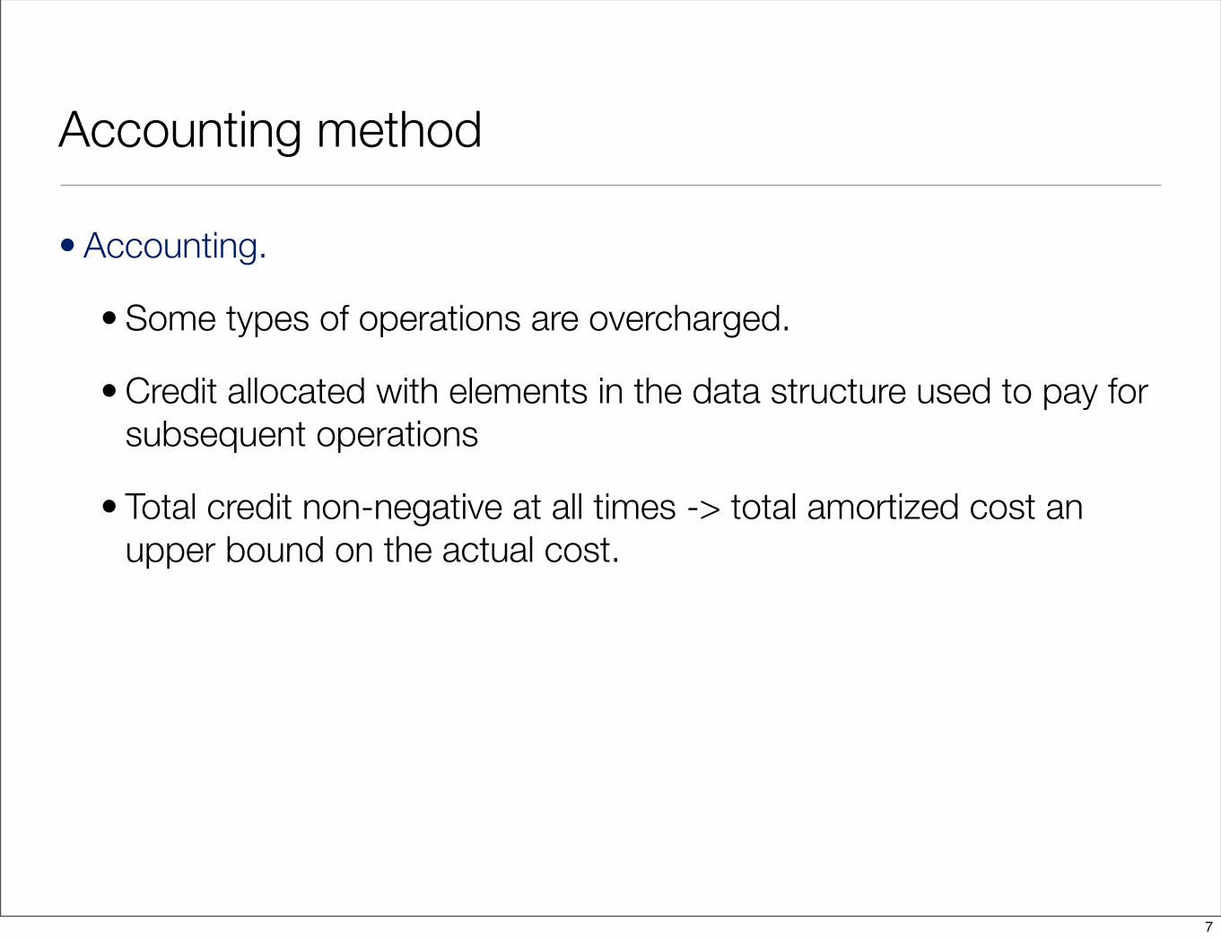
• Accounting.
• Some types of operations are overcharged.
• Credit allocated with elements in the data structure used to pay for subsequent operations
• Total credit non-negative at all times -> total amortized cost an upper bound on the actual cost.
7

Dynamic Tables
• Amortized costs:
• Amortized cost of insertion: 3
• 1 for own insertion
• 1 for its first reinsertion.
• 1 to pay for reinsertion of one of the items that have already been reinserted once.
8

Dynamic Tables
• Analysis: keep 2 credits on each element in the array that is beyond the middle.
• table not full: insert costs 1, and we have 2 credits to save.
• table full, i.e., doubling: half of the elements have 2 credits each. Use these to pay for reinsertion of all in the new array.
• Amortized cost per operation: 3.2 2 2
x x x x x x x x x x x
2 2 2 2 2 2 2 2
x x x x x x x x x x x x x x x x
x x x x x x x x x x x x x x x x
9

Example: Stack with MultiPop
• Stack with MultiPop.• Push(e): push element e onto stack.• MultiPop(k): pop top k elements from the stack
• Worst case: Implement via linked list or array.• Push: O(1).• MultiPop: O(k).
• Amortized cost per operation: 2.
10

Stack: Aggregate Analysis
• Amortized analysis. Sequence of n Push and MultiPop operations.• Each object popped at most once for each time it is pushed.• #pops on non-empty stack ≤ #Push operations ≤ n.• Total time O(n).
• Amortized cost per operation: 2n/n = 2.
11
Stack: Accounting Method
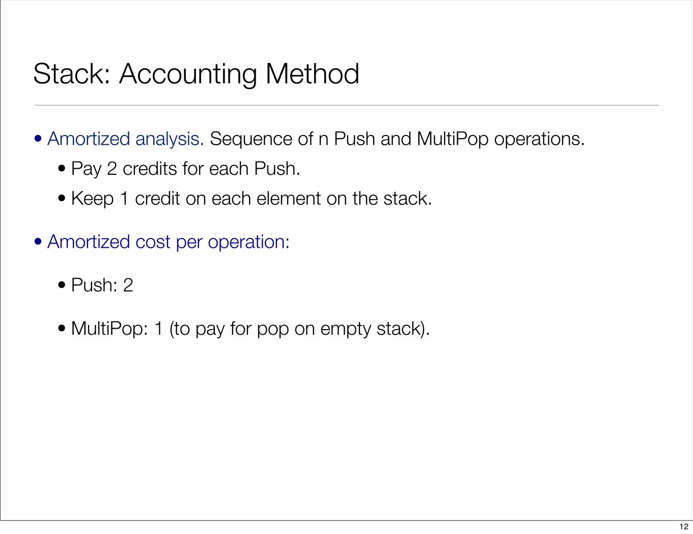
• Amortized analysis. Sequence of n Push and MultiPop operations.• Pay 2 credits for each Push.• Keep 1 credit on each element on the stack.
• Amortized cost per operation:
• Push: 2
• MultiPop: 1 (to pay for pop on empty stack).
12
Potential method
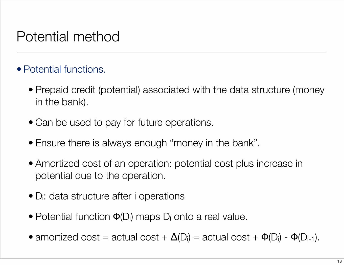
• Potential functions.
• Prepaid credit (potential) associated with the data structure (money in the bank).
• Can be used to pay for future operations.
• Ensure there is always enough “money in the bank”.
• Amortized cost of an operation: potential cost plus increase in potential due to the operation.
• Di: data structure after i operations
• Potential function Φ(Di) maps Di onto a real value.
• amortized cost = actual cost + Δ(Di) = actual cost + Φ(Di) - Φ(Di-1).
13

Potential Functions
• Amortized cost:
• amortized cost = actual cost + Δ(Di) = actual cost + Φ(Di) - Φ(Di-1).
• Stack.
•Φ(Di) = #elements on the stack.
• amortized cost of Push = 1 + Δ(Di) = 2.
• amortized cost of MultiPop(k): If k’=min(k,|S|) elements are popped.
• if S ≠ ∅: amortized cost = k‘+ Φ(Di) -Φ(Di-1) = k’ - k’ = 0.
• if S = ∅: amortized cost = 1 + Δ(Di) = 1.
14

Potential Functions
• Amortized cost:
• amortized cost = actual cost + Δ(Di) = actual cost + Φ(Di) - Φ(Di-1).
• Dynamic tables
•Φ(Di) =
• L = current array size, k = number of elements in array.
• amortized cost of insertion:
• Array not full: amortized cost = 1 + 2 = 3
• Array full (doubling): Actual cost = L + 1, Φ(Di-1) = L, Φ(Di)=2: amortized cost = L + 1 + (2 - L) = 3.
�2(k � L/2) if k ⇥ L/20 otherwise
15

Amortized Cost vs Actual Cost
• Total cost:
• ∑ amortized cost = ∑(actual cost + Δ(Di)) =∑ actual cost + Φ(Dn) - Φ(D0).
• ∑ actual cost = ∑ amortized cost + Φ(D0) - Φ(Dn).
• If potential always nonnegative and Φ(D0) = 0 then
∑ actual cost ≤ ∑ amortized cost.
16
Potential Method
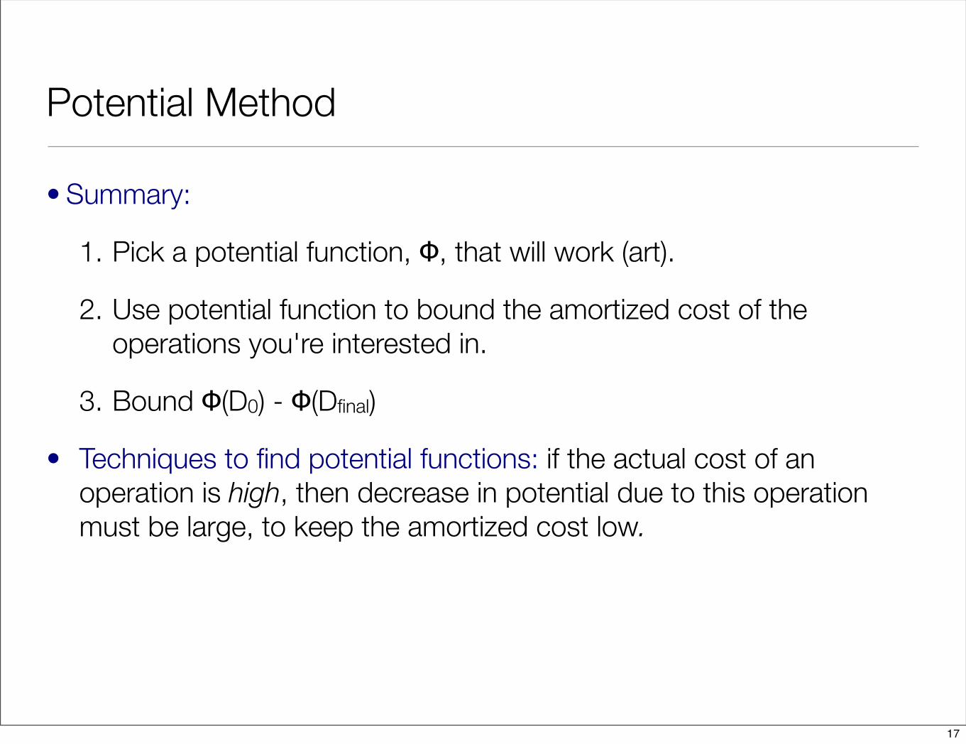
• Summary:
1. Pick a potential function, Φ, that will work (art).
2. Use potential function to bound the amortized cost of the operations you're interested in.
3. Bound Φ(D0) - Φ(Dfinal)
• Techniques to find potential functions: if the actual cost of an operation is high, then decrease in potential due to this operation must be large, to keep the amortized cost low.
17

Union-Find Data Structures
18

Union-Find Data Structure
• Union-Find data structure: • Makeset(x): Create a singleton set containing x and return its identifier.• Union(A,B): Combine the sets identified by A and B into a new set, destroying
the old sets. Return the identifier of the new set.• Find(x): Return the identifier of the set containing x.
• Only requirement for identifier: find(x) = find(y) iff x and y are in the same set.
• Applications: Connectivity, Kruskal’s algorithm for MST, ...
19
A Simple Union-Find Data Structure
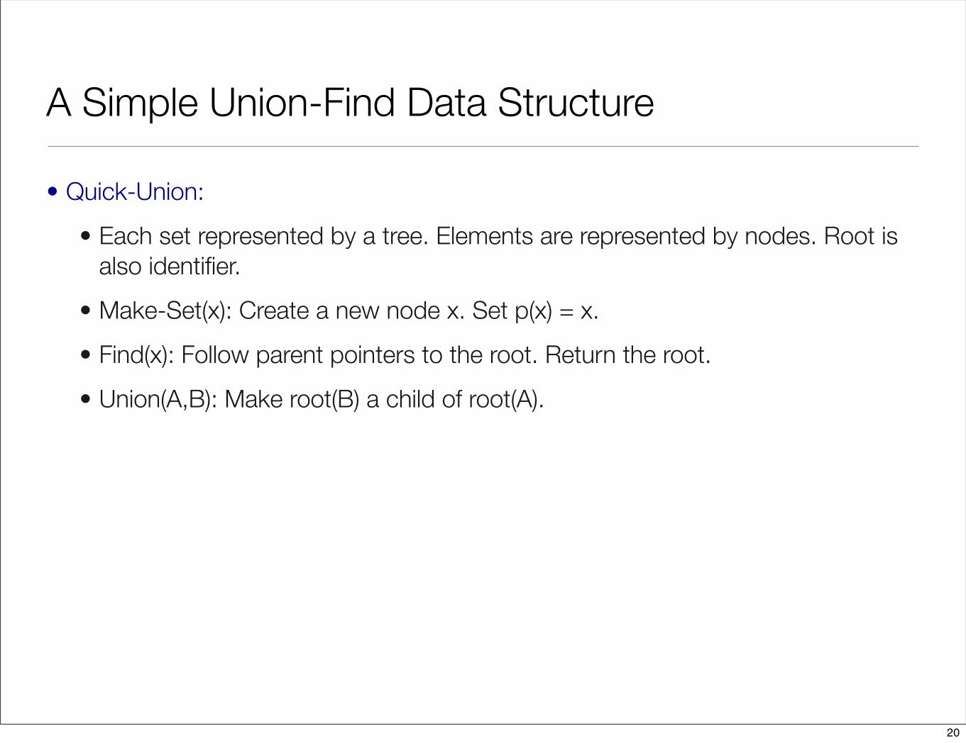
• Quick-Union:• Each set represented by a tree. Elements are represented by nodes. Root is
also identifier.• Make-Set(x): Create a new node x. Set p(x) = x.• Find(x): Follow parent pointers to the root. Return the root.• Union(A,B): Make root(B) a child of root(A).
20

A Simple Union-Find Data Structure
• Quick-Union:• Union(A,B): Make root(B) a child
of root(A).
1 2 3 4 5 6 7 8 9
1 2 3 4
5
6 7 8 9
1
2 3 4
5
6 7 8 9
1
2 3 4
5
6 7
8
9
1
2 3 4
5
6
7
8
9
Union(3,1)
Union(7,5)
Union(7,8)
Union(3,7)
21

A Simple Union-Find Data Structure
• Quick-Union:• Each set represented by a tree. Elements are represented by nodes. Root is
also identifier.• Make-Set(x): Create a new node x. Set p(x) = x.• Find(x): Follow parent pointers to the root. Return the root.• Union(A,B): Make root(B) a child of root(A).
• Analysis:• Make-Set(x) and Union(A,B): O(1)• Find(x): O(h), where h is the height of the tree containing x. Worst-case O(n).
22

A Simple Union-Find Data Structure
• Quick Find:• Each set represented by a tree of height at most one. Elements are
represented by nodes. Root is also identifier.• Make-Set(x): Create a new node x. Set p(x) = x and size(x) = 1.• Find(x): Follow parent pointer to root. Return root. • Union(A,B): Move all elements from smallest set to larger set (change parent
pointers). I.e., set p(B) = A and size(A) = size(A) + size(B).
23

A Simple Union-Find Data Structure
• Quick Find:• Union(A,B): Move all elements
from smallest set to larger set (change parent pointers).
1 2 3 4 5 6 7 8 9
1 2 3 4
5
6 7 8 9
1
2 3 4
5
6 7 8 9
1
2 3 4
5
6 7
8
9
Union(3,1)
Union(7,5)
Union(7,8)
Union(3,7)
1
2
3
4
5
6 7
8
9
24

A Simple Union-Find Data Structure
• Quick Find:• Each set represented by a tree of height at most one. Elements are
represented by nodes. Root is also identifier.• Make-Set(x): Create a new node x. Set p(x) = x and size(x) = 1.• Find(x): Follow parent pointer to root. Return root. • Union(A,B): Move all elements from smallest set to larger set (change parent
pointers). I.e., set p(B) = A and size(A) = size(A) + size(B). • Analysis:
• Make-Set(x) and Find(x): O(1)• Union(A,B): O(n)
25

Amortized Complexity of Quick-Find
• Amortized analysis: Consider a sequence of k Unions.
• Observation 1: How many elements can be touched by the k Unions?
• Consider an element x:• What can we say about the size of the set containing x before and after a
union that changes x’s parent pointer?• How large can the set containing x be after the m Unions?• How many times can x’s parent pointer be changed?
26

Amortized Complexity of Quick-Find
• Amortized analysis:• Each time x’s parent pointer changes the size of the set containing it at least
doubles.• At most 2k elements can be touched by k unions.• Size of set containing x after k unions at most 2k.• x’s parent pointer is updated at most lg(2k) times.• In total O(k log k) parent pointers updated in a sequence of k unions.• Amortized time per union: O(log k).
• Lemma. Using the Quick-Find data structure a Find operation takes worst case time O(1), a Make-Set operation time O(1), and a sequence of n Union operations takes time O(n log n).
27

A Better Union-Find Data Structure
• Union-by-Weight or Union-by-Rank.
• Union-by-Weight. Make the root of the smallest tree a child of the root of the bigger tree.
• Union-by-Rank. Each node x has an integer rank(x) associated.• Make-Set(x): Create a new node x. Set p(x) = x and rank(x) = 0. • Find(x): Follow parent pointers to the root. Return the root.• Union(A,B): 3 cases:
• rank(A) > rank(B). Make B a child of A.• rank(A) < rank(B). Make A a child of B.• rank(A) = rank(B). Make B a child of A and set rank(A) = rank(A)+1.
28

Analysis of Union-by-Rank
• Increasing ranks. • rank(x) < rank(p(x)).• A root of set containing x: Find(x) takes O(rank(A)+1) time.
• rank(A) ≤ lg n: Show |A| ≥ 2rank(A) by induction.• A=Makeset(x): rank(A)=0 and |A| = 20 = 1.• A=Union(B,C): 2 cases
• rank(A)=rank(B) or rank(A)=rank(C): ok, since set only got larger.• rank(B)=rank(C)=k and rank(A)=k+1.
|A| = |B| + |C| ≥ 2k + 2k = 2k+1.• Lemma. Using the Union-by-Rank data structure a Find operation takes worst
case time O(log n), and a Make-Set or Union operation takes time O(1).
29

Path Compression
• Path compression. After each Find(x) operation, for all nodes y on the path from x to the root, set p(y) = x.
• Example. Find(6).
1
2
3
4
5
6
7
8
9
1
2
3
4
56
7
8
9
30

Path Compression
• Path compression. After each Find(x) operation, for all nodes y on the path from x to the root, set p(y) = x.
• Tarjan: Union-by-Rank and path compression. Starting from an empty data structure the total time of n Makes-Set operations, at most n Union operations, and m Find operations takes time O(n + m α(n)).• α(n). Extremely slowly growing inverse Ackermann’s function.• Analysis complicated, but algorithm simple.• 2 one-pass variants path halving and path splitting. Same asymptotic running
time.
31

• Ackermann’s function
• Inverse Ackermann:• Grows extremely slowly.
Ackermann’s function
Ak(j) =
�j + 1 if k = 0,
A(j+1)k�1 (j) if k � 1.
�(n) = min{k : Ak(1) � n}.
32
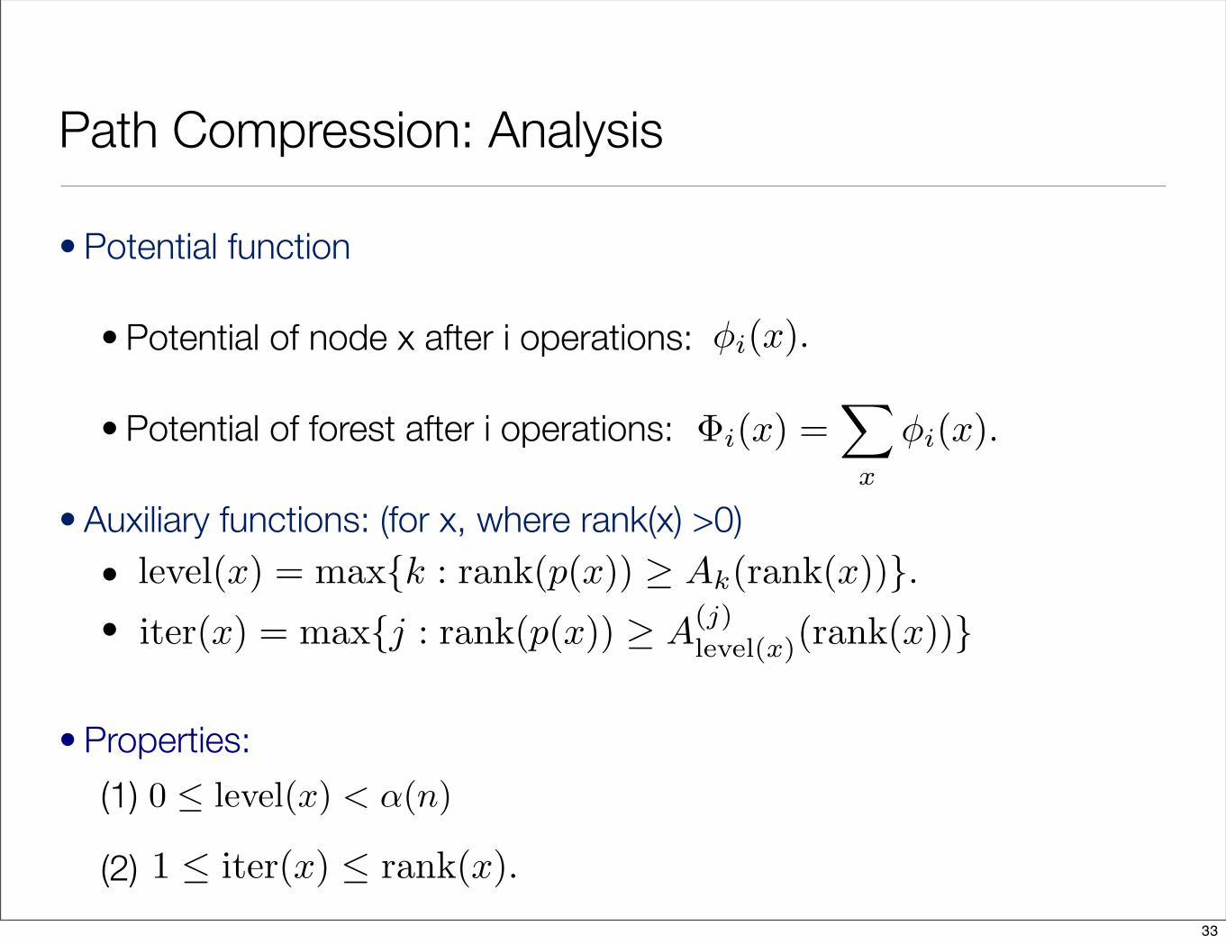
• Potential function
• Potential of node x after i operations:
• Potential of forest after i operations:
• Auxiliary functions: (for x, where rank(x) >0)• •
• Properties:(1)
(2)
Path Compression: Analysis
�i(x) =�
x
�i(x).
�i(x).
level(x) = max{k : rank(p(x)) � Ak(rank(x))}.
1 � iter(x) � rank(x).
iter(x) = max{j : rank(p(x)) � A(j)level(x)(rank(x))}
0 level(x) < ↵(n)
33

• Potential function
•
• Potential of forest after i operations:
• Properties:(1)
(2)
(3)
(4) If x not root and rank(x) > 0,
Path Compression: Analysis
�i(x) =�
x
�i(x).
1 � iter(x) � rank(x).
⇥i(x) =
��(n) · rank(x) if x root or rank(x) = 0(�(n)� level(x)) · rank(x)� iter(x) if x not root and rank(x) ⇤ 1.
0 ⇥ ⇥i(x) ⇥ �(n) · rank(x).
⇥i(x) < �(n) · rank(x).
0 level(x) < ↵(n)
34

• Potential function
•
• Potential of forest after i operations:• Makeset(x): O(1)• Union(A,B) og Find(x): O(α(n))
• Lemma 1. Suppose x not root, and ith operation Union or Find. Then• x’s potential cannot increase• if x has positive rank and iter or level changes, then x’s potential
decrease by at least 1.
Path Compression: Analysis
�i(x) =�
x
�i(x).
⇥i(x) =
��(n) · rank(x) if x root or rank(x) = 0(�(n)� level(x)) · rank(x)� iter(x) if x not root and rank(x) ⇤ 1.
35
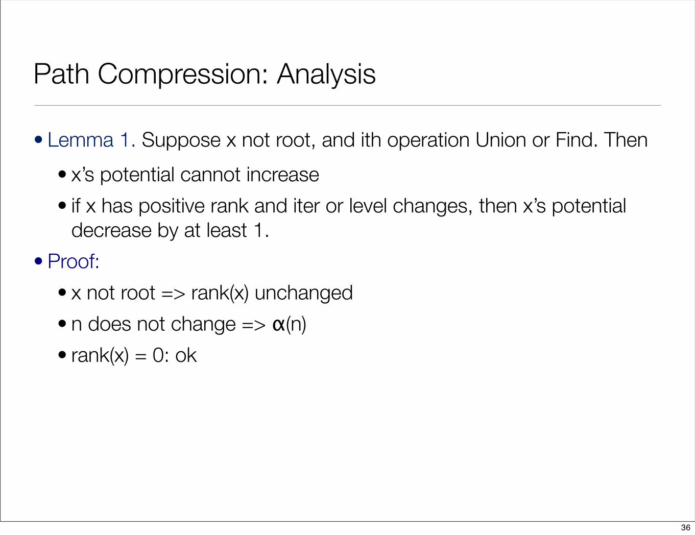
• Lemma 1. Suppose x not root, and ith operation Union or Find. Then• x’s potential cannot increase• if x has positive rank and iter or level changes, then x’s potential
decrease by at least 1.• Proof:
• x not root => rank(x) unchanged• n does not change => α(n)• rank(x) = 0: ok
Path Compression: Analysis
36

• Lemma 1. Suppose x not root, and ith operation Union or Find. Then• x’s potential cannot increase• if x has positive rank and iter or level changes, then x’s potential
decrease by at least 1.• Proof: rank(x)>0
• level increases monotonically over time• level unchanged => iter either increase or unchanged• both unchanged: ok
Path Compression: Analysis
37

• Lemma 1. Suppose x not root, and ith operation Union or Find. Then• x’s potential cannot increase• if x has positive rank and iter or level changes, then x’s potential
decrease by at least 1.• Proof: rank(x)>0
• level unchanged and iter increases: iter increase by at least 1.• level increases:
• level increases by at least 1 => (α(n)-level)rank(x)-iter(x) drops by at least rank(x).
• iter might decrease at most rank(x)-1• x’s potential decrease by at least 1.
Path Compression: Analysis
38

• Lemma 1. Suppose x not root, and ith operation Union or Find. Then• x’s potential cannot increase• if x has positive rank and iter or level changes, then x’s potential
decrease by at least 1.
• Lemma. The amortized cost of Union(A,B) is O(α(n)).• Assume B made parent of A.• Real cost 1. Show increase in potential at most α(n).• Only A’s, B’s and the children of B’s potential can change.• potential of B’s children can only decrease.• A: decreases due to property 4 (before operation it was α(n)rank(A)).• B: root both before and after. rank increase by at most 1 => potential
of B increases with at most α(n).
Path Compression: Analysis
39
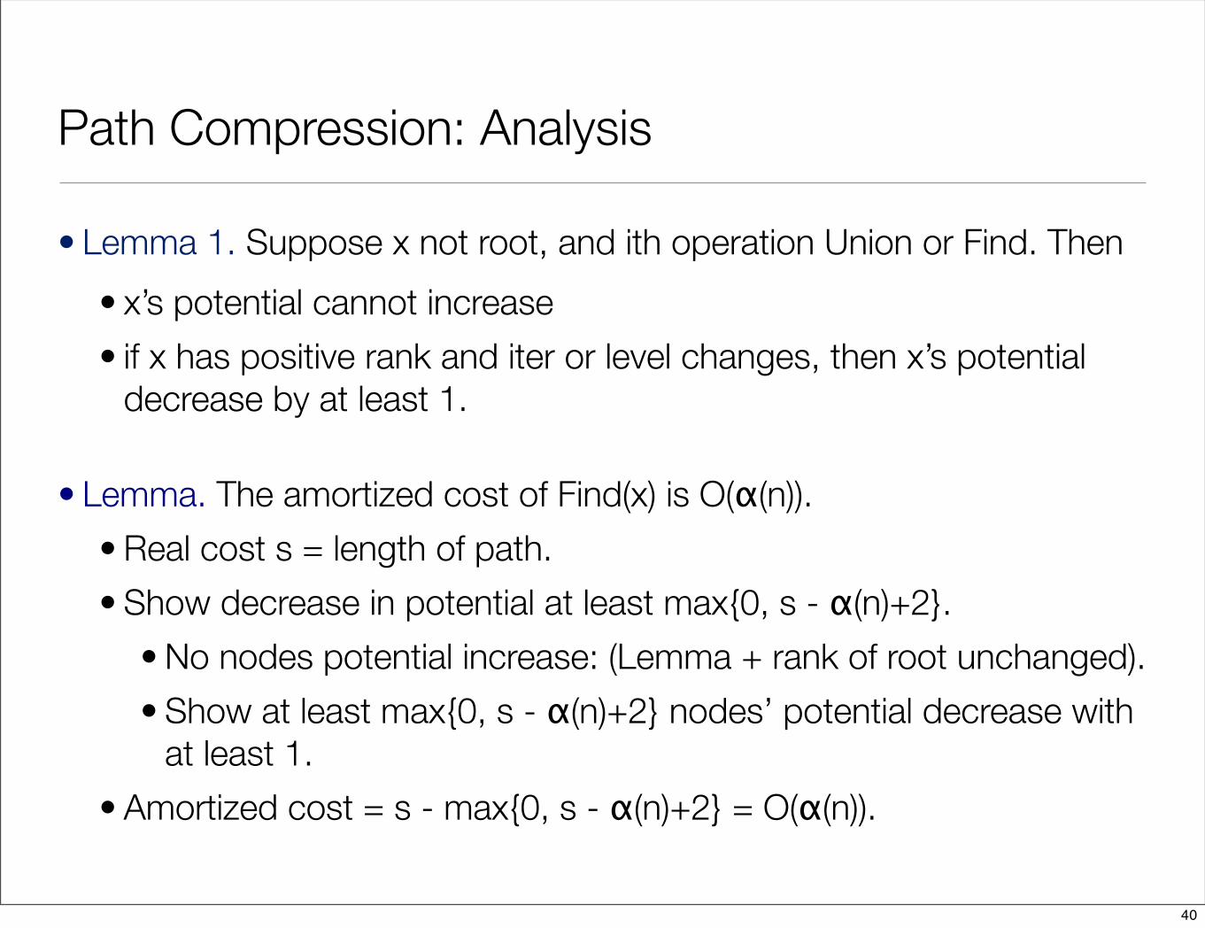
• Lemma 1. Suppose x not root, and ith operation Union or Find. Then• x’s potential cannot increase• if x has positive rank and iter or level changes, then x’s potential
decrease by at least 1.
• Lemma. The amortized cost of Find(x) is O(α(n)).• Real cost s = length of path.• Show decrease in potential at least max{0, s - α(n)+2}.
• No nodes potential increase: (Lemma + rank of root unchanged).• Show at least max{0, s - α(n)+2} nodes’ potential decrease with
at least 1.• Amortized cost = s - max{0, s - α(n)+2} = O(α(n)).
Path Compression: Analysis
40

• Show at least max{0, s - α(n)+2} nodes’ potential decrease with at least 1.• x node such that
• rank(x) > 0 • x has an ancestor y (not the root) with level(x) = level(y) before the Find
operation.• x’s potential decrease by at least 1: k = level(x), i = iter(x) before Find.• Before Find operation
• After: rank(p(x)) = rank(p(y)), rank(p(y)) not decreased, and rank(x) unchanged:
• Either iter(x) or level (x) increases. Lemma 1 implies potential of x decreases.
Path Compression: Analysis
rank(p(y)) � Ak(rank(y))
� Ak(rank(p(x))
� Ak(Aik(rank(x))
= A
(i+1)k (rank(x)).
Ak(rank(p(x))) � A
(i+1)k (rank(x))
41

Summary
• Amortized analysis.
• 2 Examples: Dynamic tables, stack with multipop.
• Union-Find Data Structure.
• Union-by-Rank + path compression: worst case + amortized bounds.
42