Amortized Analysis - Stanford...
86
Amortized Analysis
Transcript of Amortized Analysis - Stanford...

Amortized Analysis

Outline for Today
● Amortized Analysis● Analyzing data structures over the long term.
● Cartesian Trees Revisited● Why could we construct them in time O(n)?
● The Two-Stack Queue● A simple and elegant queue implementation.
● 2-3-4 Trees● A better analysis of 2-3-4 tree insertions and
deletions.

Two Worlds
● Data structures have diferent requirements in diferent contexts.● In real-time applications, each operation on a
given data structure needs to be fast and snappy.● In long data processing pipelines, we care more
about the total time used than we do the cost of any one operation.
● In many cases, we can get better performance in the long-run than we can on a per-operation basis.● Good intuition: “economy of scale.”

Key Idea: Design data structures that trade per-operation eficiency for
overall eficiency.
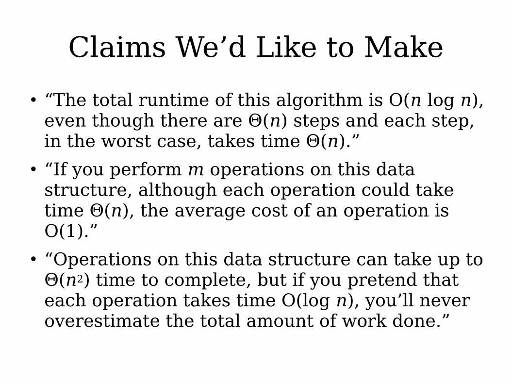
Claims We’d Like to Make
● “The total runtime of this algorithm is O(n log n), even though there are Θ(n) steps and each step, in the worst case, takes time Θ(n).”
● “If you perform m operations on this data structure, although each operation could take time Θ(n), the average cost of an operation is O(1).”
● “Operations on this data structure can take up to Θ(n2) time to complete, but if you pretend that each operation takes time O(log n), you’ll never overestimate the total amount of work done.”

What We Need
● First, we need a mathematical framework for analyzing algorithms and data structures when the costs of individual operations vary.
● Next, we need a set of design techniques for building data structures that nicely ft into this framework.
● Today is mostly about the frst of these ideas. We’ll explore design techniques all next week.

Amortized Analysis

The Goal
● Suppose we have a data structure and perform a series of m operations op₁, op₂, …, opₘ.● These operations might be the same operation, or
they might be diferent.● Let t(opₖ) denote the time required to perform
operation opₖ.● Goal: Bound this expression, which represents
the total runtime across all operations:
T=∑i=1
m
t (opi)

Amortized Analysis
● An amortized analysis is a diferent way of bounding the runtime of a sequence of operations.
● Idea: Assign to each operation opᵢ a new cost a(opᵢ), called the amortized cost, such that the following is true for any sequence of m operations:
∑i=1
m
t (opi) ≤ ∑i=1
m
a(opi)
t
a
Question: How do you choose amortized
costs?
Question: How do you choose amortized
costs?

Where We’re Going
There are three standard techniques for assigning amortized costs to operations:● The aggregate method directly assigns each
operation its average cost.
The banker’s method places credits on the data structure, which are redeemable for units of work.
The potential method assigns a potential function to the data structure, which can be charged to pay for future work or released to pay for recent work.

The Aggregate Method
● In the aggregate method, we assign each operation a cost of
a(opᵢ) = T*(m) / m
where T*(m) is the maximum amount of work done by any series of m operations.
● We essentially pretend that each operation’s runtime is the the average cost of all operations performed.

The Aggregate Method
● In the aggregate method, we assign each operation a cost of
a(opᵢ) = T*(m) / m
where T*(m) is the maximum amount of work done by any series of m operations.
● We essentially pretend that each operation’s runtime is the the average cost of all operations performed.

Cartesian Trees Revisited

Cartesian Trees
● A Cartesian tree is a binary tree derived from an array and defned as follows:
● The empty array has an empty Cartesian tree.● For a nonempty array, the root stores the minimum
value. Its left and right children are Cartesian trees for the subarrays to the left and right of the minimum.
261 268 161 167 166 14 55 22 43 116 5 3 9 7
161
261 166
167268
3
7
9
5
6
11
14
22
4355

The Runtime Analysis
● In a sequence of operations that adds n elements to a Cartesian tree, adding an individual node to a Cartesian tree might take time Θ(n).
● However, the net time spent adding new nodes across the whole tree is O(n).
● Why is this?● Every node pushed at most once.● Every node popped at most once.● Work done is proportional to the number of pushes and pops.● Total runtime is O(n).
● The amortized cost of adding a node is O(n) / n = O(1).

Where We’re Going
There are three standard techniques for assigning amortized costs to operations:
The aggregate method directly assigns each operation its average cost.
● The banker’s method places credits on the data structure, which are redeemable for units of work.
The potential method assigns a potential function to the data structure, which can be charged to pay for future work or released to pay for recent work.

The Banker's Method
● In the banker's method, operations can place credits on the data structure or spend credits that have already been placed.
● Placing a credit on the data structure takes time O(1).
● Spending a credit previously placed on the data structure takes time -O(1). (Yes, that’s negative time!)
● The amortized cost of an operation is then
a(opᵢ) = t(opᵢ) + O(1) · (addedᵢ – removedᵢ)
● There aren’t any real credits anywhere. They’re just an accounting trick.
t
a
+ – + + + – –

The Banker's Method
● If we never spend credits we don't have:
● The sum of the amortized costs upper-
bounds the sum of the true costs.
∑i=1
k
a(opi) = ∑i=1
k
(t (opi)+O(1)⋅(addedi−removedi))
= ∑i=1
k
t (opi) + O(1)∑i=1
k
(addedi−removedi)
= ∑i=1
k
t (opi) + O(1)⋅netCredits
≥ ∑i=1
k
t (opi)

Constructing Cartesian Trees
271 137 159 314 42
271
271
$
Work done: 1 pushCredits Added: $1
Amortized Cost: 2
Work done: 1 pushCredits Added: $1
Amortized Cost: 2

Constructing Cartesian Trees
271 137 159 314 42
271
137
137
$
Work done: 1 push, 1 popCredits Removed: $1
Credits Added: $1
Amortized Cost: 2
Work done: 1 push, 1 popCredits Removed: $1
Credits Added: $1
Amortized Cost: 2

Constructing Cartesian Trees
271 137 159 314 42
271
137
137
$
159
159
$
Work done: 1 pushCredits Added: $1
Amortized Cost: 2
Work done: 1 pushCredits Added: $1
Amortized Cost: 2

Constructing Cartesian Trees
271 137 159 314 42
271
137
137
$
159
159
$
314
314
$
Work done: 1 pushCredits Added: $1
Amortized Cost: 2
Work done: 1 pushCredits Added: $1
Amortized Cost: 2

Constructing Cartesian Trees
271 137 159 314 42
271
137
159
314
42
42
$
Work done: 1 push, 3 popsCredits Removed: $3
Credits Added: $1
Amortized Cost: 2
Work done: 1 push, 3 popsCredits Removed: $3
Credits Added: $1
Amortized Cost: 2

The Banker's Method
● Using the banker's method, the cost of an insertion is
= t(op) + O(1) · (addedᵢ – removedᵢ)
= 1 + k + O(1) · (1 – k)
= 1 + k + 1 – k
= 2
= O(1)● Each insertion has amortized cost O(1).● Any n insertions will take time O(n).

Intuiting the Banker's Method
271 137 159 314 42
Push 271 Push 137
Pop 271
Push 159 Push 314 Push 42
Pop 314
Pop 159
Pop 137

Intuiting the Banker's Method
271 137 159 314 42
Push 271 Push 137
Pop 271
Push 159 Push 314 Push 42
Pop 314Pop 159Pop 137
Each operation here is being “charged” for two units of work,
even if didn't actually do two units of work.
Each operation here is being “charged” for two units of work,
even if didn't actually do two units of work.

Intuiting the Banker's Method
271 137 159 314 42
Push 271 Push 137
Pop 271
Push 159 Push 314 Push 137
Pop 314
Pop 159
Pop 137
$$
$ $
$

Intuiting the Banker's Method
271 137 159 314 42
Push 271 Push 137
Pop 271
Push 159 Push 314 Push 137
Pop 314Pop 159Pop 137
$
Each credit placed can be used to “move” a unit of work from one
operation to another.
Each credit placed can be used to “move” a unit of work from one
operation to another.

An Observation
● We defned the amortized cost of an operation to be
a(opᵢ) = t(opᵢ) + O(1) · (addedᵢ – removedᵢ)
● Equivalently, this is
a(opᵢ) = t(opᵢ) + O(1) · Δcreditsᵢ
● Some observations:
● It doesn't matter where these credits are placed or removed from.
● The total number of credits added and removed doesn't matter; all that matters is the diference between these two.

Where We’re Going
There are three standard techniques for assigning amortized costs to operations:
The aggregate method directly assigns each operation its average cost.
The banker’s method places credits on the data structure, which are redeemable for units of work.
● The potential method assigns a potential function to the data structure, which can be charged to pay for future work or released to pay for recent work.

The Potential Method
● In the potential method, we defne a potential function Φ that maps a data structure to a non-negative real value.
● Each operation may change this potential.
● If we denote by Φᵢ the potential of the data structure just before operation i, then we can defne a(opᵢ) as
a(opᵢ) = t(opᵢ) + O(1) · (Φᵢ₊₁ – Φᵢ)
● Intuitively, operations that increase the potential have amortized cost greater than their true cost, and operations that decrease the potential have amortized cost less than their true cost.
t
a
+1 -1 +1 +1 0 0 -2 +1

The Potential Method
● Assuming that Φₖ₊₁ – Φ₁ ≥ 0, this means that the sum of the amortized costs upper-bounds the sum of the real costs.
● Typically, Φ₁ = 0, so Φₖ₊₁ – Φ₁ ≥ 0 holds.
∑i=1
k
a(opi) = ∑i=1
k
(t (opi)+O(1)⋅(Φi+1−Φi))
= ∑i=1
k
t (opi) + O(1)⋅∑i=1
k
(Φi+1−Φi)
= ∑i=1
k
t (opi) + O(1)⋅(Φk+1−Φ1)

Constructing Cartesian Trees
271 137 159 314 42
271
271
Work done: 1 pushΔΦ: +1
Amortized Cost: 2
Work done: 1 pushΔΦ: +1
Amortized Cost: 2
Φ = 1

Constructing Cartesian Trees
271 137 159 314 42
271
137
137
Work done: 1 push, 1 popΔΦ: 0
Amortized Cost: 2
Work done: 1 push, 1 popΔΦ: 0
Amortized Cost: 2
Φ = 1
Notice that Φ went
1 → 0 → 1
All that matters is the net change.
Notice that Φ went
1 → 0 → 1
All that matters is the net change.
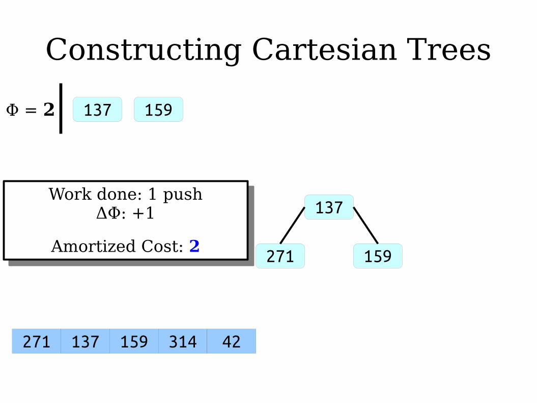
Constructing Cartesian Trees
271 137 159 314 42
271
137
137
159
159
Work done: 1 pushΔΦ: +1
Amortized Cost: 2
Work done: 1 pushΔΦ: +1
Amortized Cost: 2
Φ = 2

Constructing Cartesian Trees
271 137 159 314 42
271
137
137
159
159
314
314
Work done: 1 pushCredits Added: ΔΦ: +1
Amortized Cost: 2
Work done: 1 pushCredits Added: ΔΦ: +1
Amortized Cost: 2
Φ = 3

Constructing Cartesian Trees
271 137 159 314 42
271
137
159
314
42
42
Work done: 1 push, 3 popsΔΦ: -2
Amortized Cost: 2
Work done: 1 push, 3 popsΔΦ: -2
Amortized Cost: 2
Φ = 1

The Potential Method
● Using the potential method, the cost of an insertion into a Cartesian tree can be computed as
= t(op) + ΔΦ
= 1 + k + O(1) · (1 – k)
= 1 + k + 1 – k
= 2
= O(1)● So the amortized cost of an insertion is O(1).● Therefore, n total insertions takes time O(n).

Amortization in Practice:The Two-Stack Queue

The Two-Stack Queue
● Maintain two stacks, an In stack and an Out stack.
● To enqueue an element, push it onto the In stack.
● To dequeue an element:● If the Out stack is empty, pop everything of
the In stack and push it onto the Out stack.● Pop the Out stack and return its value.

An Aggregate Analysis
● Claim: The amortized cost of popping an element is O(1).
● Proof:● Every value is pushed onto a stack at most
twice: once for in, once for out.● Every value is popped of of a stack at most
twice: once for in, once for out.● Each push/pop takes time O(1).● Net runtime: O(n).● Amortized cost: O(n) / n = O(1).

The Banker's Method
● Let's analyze this data structure using the banker's method.
● Some observations:● All enqueues take worst-case time O(1).● Each dequeue can be split into a “light” or
“heavy” dequeue.● In a “light” dequeue, the out stack is nonempty.
Worst-case time is O(1).● In a “heavy” dequeue, the out stack is empty.
Worst-case time is O(n).

The Two-Stack Queue
1Out In
2
3
4
$
$
$
$

The Two-Stack Queue
1
In
2
3
4Out

The Banker's Method
● Enqueue:● O(1) work, plus one credit added.● Amortized cost: O(1).
● “Light” dequeue:● O(1) work, plus no change in credits.● Amortized cost: O(1).
● “Heavy” dequeue:● Θ(k) work, where k is the number of entries that started
in the “in” stack.● k credits spent.● By choosing the amount of work in a credit
appropriately, amortized cost is O(1).

The Potential Method
● Defne Φ(D) to be the height of the in stack.● Enqueue:
● Does O(1) work and increases Φ by one.● Amortized cost: O(1).
● “Light” dequeue:● Does O(1) work and leaves Φ unchanged.● Amortized cost: O(1).
● “Heavy” dequeue:● Does Θ(k) work, where k is the number of entries moved from
the “in” stack.● ΔΦ = -k.● By choosing the amount of work stored in each unit of potential
correctly, amortized cost becomes O(1).

Time-Out for Announcements!

Problem Sets
● Problem Set Two solutions are now up on the course website.● The TAs are hard at work grading everything.
We’ll try to get everything back as soon as possible!
● Problem Set Three is due next Thursday, May 3rd, at 2:30PM.● Have questions? Stop by ofice hours or ask
them on Piazza!

Grace Hopper Conference
● Applications are now open for CS department funding to attend next year’s Grace Hopper Conference● (September 26 – 28, Houston, TX)
● Phenomenal opportunity for anyone interested.
● Apply online using this link.

Back to CS166!
Another Example: 2-3-4 Trees

2-3-4 Trees
● Inserting or deleting values from a 2-3-4 trees takes time O(log n).
● Why is that?● We do some amount of work fnding the insertion
or deletion point, which is Θ(log n).● We also do some amount of work “fxing up” the
tree by doing insertions or deletions.● What is the cost of that second amount of
work?

2-3-4 Tree Insertions
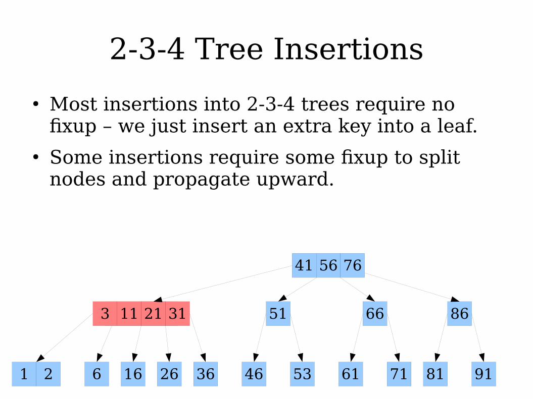
● Most insertions into 2-3-4 trees require no fxup – we just insert an extra key into a leaf.
● Some insertions require some fxup to split nodes and propagate upward.
1 6
11 21 31
41
16 91
86
26 36 81
56
53
51
46
76
71
66
612

2-3-4 Tree Insertions
● Most insertions into 2-3-4 trees require no fxup – we just insert an extra key into a leaf.
● Some insertions require some fxup to split nodes and propagate upward.
1 6
11 21 31
41
16 91
86
26 36 81
56
53
51
46
76
71
66
612 3
2-3-4 Tree Insertions
● Most insertions into 2-3-4 trees require no fxup – we just insert an extra key into a leaf.
● Some insertions require some fxup to split nodes and propagate upward.
1 6
11 21 31
41
16 91
86
26 36 81
56
53
51
46
76
71
66
612
3

2-3-4 Tree Insertions
● Most insertions into 2-3-4 trees require no fxup – we just insert an extra key into a leaf.
● Some insertions require some fxup to split nodes and propagate upward.
1 6
11 31
41
16 91
86
26 36 81
56
53
51
46
76
71
66
612
3
21

2-3-4 Tree Insertions
● Most insertions into 2-3-4 trees require no fxup – we just insert an extra key into a leaf.
● Some insertions require some fxup to split nodes and propagate upward.
1 6
11 31
16 91
86
26 36 81
56
53
51
46
76
71
66
612
3
21
41
Observation: The only case where an insertion propagates upward is when there are four keys in a node.
Observation: The only case where an insertion propagates upward is when there are four keys in a node.

2-3-4 Tree Deletions
36
46
31 41 61
56
51
● Most deletions from a 2-3-4 tree require no fxup; we just delete a key from a leaf.
● Some deletions require fxup work to propagate the deletion upward in the tree.

2-3-4 Tree Deletions
36
46
? 41 61
56
51
● Most deletions from a 2-3-4 tree require no fxup; we just delete a key from a leaf.
● Some deletions require fxup work to propagate the deletion upward in the tree.

2-3-4 Tree Deletions
?
46
41 61
56
51
● Most deletions from a 2-3-4 tree require no fxup; we just delete a key from a leaf.
● Some deletions require fxup work to propagate the deletion upward in the tree.
36

2-3-4 Tree Deletions
41 61
56
51
● Most deletions from a 2-3-4 tree require no fxup; we just delete a key from a leaf.
● Some deletions require fxup work to propagate the deletion upward in the tree.
36
46
Observation: The only case where a deletion propagates upward is when there are two sibling nodes that each have one key.
Observation: The only case where a deletion propagates upward is when there are two sibling nodes that each have one key.

2-3-4 Tree Fixup
● Claim: The fxup work on 2-3-4 trees is amortized O(1).
● We'll prove this in three steps:● First, we'll prove that in any sequence of m
insertions, the amortized fxup work is O(1).● Next, we'll prove that in any sequence of m
deletions, the amortized fxup work is O(1).● Finally, we'll show that in any sequence of
insertions and deletions, the amortized fxup work is O(1).

2-3-4 Tree Insertions
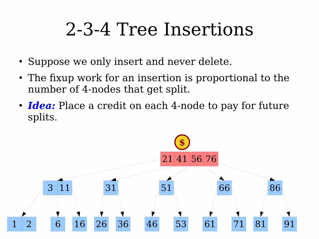
● Suppose we only insert and never delete.● The fxup work for an insertion is proportional to the
number of 4-nodes that get split.● Idea: Place a credit on each 4-node to pay for future
splits.
1 6
11 21 31
41
16 91
86
26 36 81
56
53
51
46
76
71
66
612
$
$
$

2-3-4 Tree Insertions
● Suppose we only insert and never delete.● The fxup work for an insertion is proportional to the
number of 4-nodes that get split.● Idea: Place a credit on each 4-node to pay for future
splits.
1 6
11 21 31
41
16 91
86
26 36 81
56
53
51
46
76
71
66
612 3
$
$
$

2-3-4 Tree Insertions
● Suppose we only insert and never delete.● The fxup work for an insertion is proportional to the
number of 4-nodes that get split.● Idea: Place a credit on each 4-node to pay for future
splits.
1 6
11 21 31
41
16 91
86
26 36 81
56
53
51
46
76
71
66
612
3
$
$
2-3-4 Tree Insertions
● Suppose we only insert and never delete.● The fxup work for an insertion is proportional to the
number of 4-nodes that get split.● Idea: Place a credit on each 4-node to pay for future
splits.
1 6
11 31
41
16 91
86
26 36 81
56
53
51
46
76
71
66
612
3
21
$

2-3-4 Tree Insertions
● Suppose we only insert and never delete.● The fxup work for an insertion is proportional to the
number of 4-nodes that get split.● Idea: Place a credit on each 4-node to pay for future
splits.
1 6
11 31
16 91
86
26 36 81
56
53
51
46
76
71
66
612
3
21
41

2-3-4 Tree Insertions
● Using the banker's method, we get that pure insertions have O(1) amortized fxup work.
● Could also do this using the potential method.● Defne Φn to be the number of 4-nodes.● Each “light” insertion might introduce a new 4-
node, requiring amortized O(1) work.● Each “heavy” insertion splits k 4-nodes and
decreases the potential by k for O(1) amortized work.

2-3-4 Tree Deletions
36
46
31 41 61
56
51
● Suppose we only delete and never insert.● The fxup work per layer is O(1) and only propagates
if we combine three 2-nodes together into a 4-node.● Idea: Place a credit on each 2-node whose children
are 2-nodes (call them “tiny triangles.”)
$$
$

2-3-4 Tree Deletions
36
46
? 41 61
56
51
● Suppose we only delete and never insert.● The fxup work per layer is O(1) and only propagates
if we combine three 2-nodes together into a 4-node.● Idea: Place a credit on each 2-node whose children
are 2-nodes (call them “tiny triangles.”)
$$
$

2-3-4 Tree Deletions
?
46
41 61
56
51
● Suppose we only delete and never insert.● The fxup work per layer is O(1) and only propagates
if we combine three 2-nodes together into a 4-node.● Idea: Place a credit on each 2-node whose children
are 2-nodes (call them “tiny triangles.”)
36
$$
$

2-3-4 Tree Deletions
41 61
56
51
● Suppose we only delete and never insert.● The fxup work per layer is O(1) and only propagates
if we combine three 2-nodes together into a 4-node.● Idea: Place a credit on each 2-node whose children
are 2-nodes (call them “tiny triangles.”)
36
46

2-3-4 Tree Deletions
● Using the banker's method, we get that pure deletions have O(1) amortized fxup work.
● Could also do this using the potential method.● Defne Φn to be the number of 2-nodes with two
2-node children (call these “tiny triangles.”)● Each “light” deletion might introduce two tiny
triangles: one at the node where the deletion ended and one right above it. Amortized time is O(1).
● Each “heavy” deletion combines k tiny triangles and decreases the potential by at least k. Amortized time is O(1).

Combining the Two
● We've shown that pure insertions and pure deletions require O(1) amortized fxup time.
● What about interleaved insertions and deletions?
● Initial idea: Use a potential function that's the sum of the two previous potential functions.
● Φn is the number of 4-nodes plus the number of tiny triangles.
( ) ( )# + #Φn =

A Potential Issue
1 6
11 21 31
41
16 91
86
26 36 81
56
53
51
46
76
71
66
612
= 6
( ) ( )# + #Φn =

A Potential Issue
1 6
11 21 31
41
16 91
86
26 36 81
56
53
51
46
76
71
66
612 3
( ) ( )# + #Φn =

A Potential Issue
1 6
11
16 91
86
81
56
76
71
66
612
3
21 41
( ) ( )# + #Φn =
= 5
31
26 36 53
51
46
These two “tiny triangles” are new!
These two “tiny triangles” are new!

A Problem
● When doing a “heavy” insertion that splits multiple 4-nodes, the resulting nodes might produce new “tiny triangles.”
● Symptom: Our potential doesn't drop nearly as much as it should, so we can't pay for future operations. Amortized cost of the operation works out to Θ(log n), not O(1) as we hoped.
● Root Cause: Splitting a 4-node into a 2-node and a 3-node might introduce new “tiny triangles,” which in turn might cause future deletes to become more expensive.

The Solution
● 4-nodes are troublesome for two separate reasons:● They cause chained splits in an insertion.● After an insertion, they might split and produce a
tiny triangle.● Idea: Charge each 4-node for two diferent costs:
the cost of an expensive insertion, plus the (possible) future cost of doing an expensive deletion.
( ) ( )2# + #Φn =

Unlocking our Potential
1 6
11 21 31
41
16 91
86
26 36 81
56
53
51
46
76
71
66
612
( ) ( )2# + #Φn =
= 9

Unlocking our Potential
1 6
11 21 31
41
16 91
86
26 36 81
56
53
51
46
76
71
66
612 3
( ) ( )2# + #Φn =

Unlocking our Potential
1 6
11 31
16 91
86
26 36 81
56
53
51
46
76
71
66
612
3
21 41
= 5
( ) ( )2# + #Φn =

The Solution
● This new potential function ensures that if an insertion chains up k levels, the potential drop is at least k (and possibly up to 2k).
● Therefore, the amortized fxup work for an insertion is O(1).
● Using the same argument as before, deletions require amortized O(1) fxups.

Why This Matters
● Via the isometry, red/black trees have O(1) amortized fxup per insertion or deletion.
● In practice, this makes red/black trees much faster than other balanced trees on insertions and deletions, even though other balanced trees can be better balanced.

More to Explore
● A finger tree is a variation on a B-tree in which certain nodes are pointed at by “fngers.” Insertions and deletions are then done only around the fngers.
● Because the only cost of doing an insertion or deletion is the fxup cost, these trees have amortized O(1) insertions and deletions.
● They're often used in purely functional settings to implement queues and deques with excellent runtimes.
● Liked the previous analysis? Consider looking into this for your fnal project!

Next Time
● Binomial Heaps● A simple and versatile heap data structure
based on binary arithmetic.● Lazy Binomial Heaps
● Rejiggering binomial heaps for fun and proft.


![binary heap, d-ary heap, binomial heap, amortized analysis ... · Amortized Complexity [amortizovaná složitost] In an amortized analysis , the time required to perform a sequence](https://static.fdocuments.in/doc/165x107/5ed29bc1016d386359233e54/binary-heap-d-ary-heap-binomial-heap-amortized-analysis-amortized-complexity.jpg)