All-Pass-Filter-Based PLL Systems: Linear Modeling ...

Aalborg Universitet

All-Pass-Filter-Based PLL Systems

Linear Modeling, Analysis, and Comparative Evaluation

Golestan, Saeed; Guerrero, Josep M.; Vasquez, Juan C.; Abusorrah, Abdullah M.; Al-Turki,YusufPublished in:IEEE Transactions on Power Electronics

DOI (link to publication from Publisher):10.1109/TPEL.2019.2937936

Creative Commons LicenseCC BY 4.0

Publication date:2020

Document VersionAccepted author manuscript, peer reviewed version

Link to publication from Aalborg University

Citation for published version (APA):Golestan, S., Guerrero, J. M., Vasquez, J. C., Abusorrah, A. M., & Al-Turki, Y. (2020). All-Pass-Filter-Based PLLSystems: Linear Modeling, Analysis, and Comparative Evaluation. IEEE Transactions on Power Electronics ,35(4), 3558-3572. [8818308]. https://doi.org/10.1109/TPEL.2019.2937936

General rightsCopyright and moral rights for the publications made accessible in the public portal are retained by the authors and/or other copyright ownersand it is a condition of accessing publications that users recognise and abide by the legal requirements associated with these rights.

? Users may download and print one copy of any publication from the public portal for the purpose of private study or research. ? You may not further distribute the material or use it for any profit-making activity or commercial gain ? You may freely distribute the URL identifying the publication in the public portal ?

Take down policyIf you believe that this document breaches copyright please contact us at [email protected] providing details, and we will remove access tothe work immediately and investigate your claim.

Downloaded from vbn.aau.dk on: December 06, 2021

https://doi.org/10.1109/TPEL.2019.2937936

https://vbn.aau.dk/en/publications/cbfa7690-818f-48dd-85f3-b9660417664e

https://doi.org/10.1109/TPEL.2019.2937936

0885-8993 (c) 2019 IEEE. Personal use is permitted, but republication/redistribution requires IEEE permission. See http://www.ieee.org/publications_standards/publications/rights/index.html for more information.

This article has been accepted for publication in a future issue of this journal, but has not been fully edited. Content may change prior to final publication. Citation information: DOI 10.1109/TPEL.2019.2937936, IEEETransactions on Power Electronics

All-Pass-Filter-Based PLL Systems: LinearModeling, Analysis, and Comparative Evaluation

Saeed Golestan, Senior Member, IEEE, Josep M. Guerrero, Fellow, IEEE, Juan C. Vasquez, Senior Member,IEEE, Abdullah M. Abusorrah, Senior Member, IEEE, and Yusuf Al-Turki, Senior Member, IEEE

Abstract—All-pass filter (APF) passes all frequency compo-nents of a signal without altering their amplitude, but changestheir phase. This feature has made the APF a versatile buildingblock in different signal processing applications. The focus ofthis paper is on APF-based phase-locked loops (PLLs), wherethe APF is required for creating a 90◦ phase shift at the fun-damental frequency. Such a phase shift is needed for generatinga fictitious orthogonal signal in single-phase applications andrejecting the grid voltage imbalance in three-phase systems. Tothe best of authors’ knowledge, none of the APF-based PLLshave an accurate model yet. This gap in knowledge makes theanalysis of these synchronization systems and identifying theiradvantages/disadvantages compared to state-of-the-art structurescomplicated. The main objective of this paper is to bridge thisknowledge gap.

Index Terms—All-pass filter (APF), modeling, phase-lockedloop (PLL), quadrature signal generation (QSG), single-phasesystems, synchronization, three-phase systems.

I. INTRODUCTION

POWER ELECTRONIC converters are widely used indifferent applications, such as renewable energy systems,

uninterruptible power supplies, power quality conditioners,and electric vehicles among others [1], [2]. Depending onthe application in hand, these converters may have differentcontrol systems. Almost all of them, however, require asynchronization unit in their controllers. Such a unit may bedesigned in different ways. A popular method is using thephase-locked loop (PLL) concept [3]–[5].

PLLs are nonlinear closed-loop control systems with a longhistory of use in power and energy applications. Focusing onsingle-phase applications, PLLs are divided into two major cat-egories [3]: Quadration signal generation-based PLLs (QSG-PLLs), which mimic the operating principle of a three-phasesynchronous reference frame PLL (SRF-PLL) by producinga 90◦-phase-shifted version of the single-phase input signal,and power-based PLLs (pPLLs), which employ a product-typephase detector. In power applications, which this paper focuseson, QSG-PLLs have received more attention than pPLLs [3].

Manuscript received May 14, 2018; accepted July 15, 2019.S. Golestan, J. M. Guerrero, and J. C. Vasquez are with the Department of

Energy Technology, Aalborg University, Aalborg DK-9220, Denmark (e-mail:[email protected]; [email protected]; [email protected]).

A. M. Abusorrah and Y. Al-Turki are with the Department of Electrical andComputer Engineering, Faculty of Engineering, and Center of Research Excel-lence in Renewable Energy and Power Systems, King Abdulaziz University,Jeddah, Saudi Arabia (e-mail: [email protected]; [email protected]).

Color versions of one or more of the figures in this paper are availableonline at http://ieeexplore.ieee.org.

v

APF

1s

dqn

qv

dv

sincos

iks

pk

1s

SRF‐PLL

Optional LPF

1V

1

d

ds

q

qs

1v

1v

Fig. 1. Block diagram of the 1φ-APF-PLL. v is the single-phase inputsignal. kp and ki are the control parameters of the proportional-integral (PI)controller. ωd and ωq are the cutoff frequency of low-pass filters (LPFs) inthe d- and q-axis, respectively. The q-axis LPF is optional. ωn is the nominalangular frequency of the input signal. ω and ω are both estimations of theinput signal angular frequency, and θ1 and V1 are estimations of its phaseangle and amplitude, respectively.

dqn

qv

dv

sincos

iks

pk

1s

SRF‐PLL

1V

1

d

ds

1v

1v

v

1s

kk

MFOF Optional LPF

q

qs

Fig. 2. Block diagram of the MFOF-PLL. The parameter k is an additionaldegree of freedom. See the caption of Fig. 1 for the description of otherparameters.

A large number of QSG-PLLs have been presented in theliterature [3]. The key difference between these PLLs lies inhow to produce the quadrature signal mentioned above. Usingtransfer delay [6], [7], second-order generalized integrator [8]–[10], inverse Park transform [10], [11], and all-pass filter(APF) [12]–[14] are notable examples.

The APF is a filter that passes all frequency componentswithout affecting their amplitude, but changes their phase.Using the APF for generating the quadrature signal in single-phase PLLs dates back to more than a decade ago [12]–[14].Fig. 1 illustrates the block diagram of the single-phase APF-based PLL (1φ-APF-PLL), which consists of a first-order APFfor generating the quadrature signal and an SRF-PLL. Noticethat the SRF-PLL has an optional LPF in its q-axis. Noticealso that a frequency feedback loop, which is connected tothe output of the PI controller, adapts the APF to frequencychanges.

In [15], adding a degree of freedom (parameter k) to the1φ-APF-PLL structure has been proposed. Fig. 2 illustratesthis idea, which is referred to as the modified first-order filter-



APF‐based FFPS component detector

vAPF

APFv

dqn

qv

dv

sincos

iks

pk

1s

SRF‐PLL

0.5

0.5 v

v

abc

av

bv

cv

1v

1v

Optional LPF

1V

1

d

ds

q

qs

Fig. 3. Block diagram of the 3φ-APF-PLL.

based PLL (MFOF-PLL) [15].1 Notice that the 1φ-APF-PLLis a special case of the MFOF-PLL with k = 1. Notice alsothat the MFOF frequency response converges to that of anintegrator and differentiator when the parameter k tends tozero and infinity, respectively.

The APF application is not limited to single-phase PLLs. Infact, around two decades ago, its application for rejecting thegrid voltage imbalance in three-phase PLLs has been proposedin [16]. Fig. 3 illustrates this idea, which is referred to as thethree-phase APF-based PLL (3φ-APF-PLL).2 The 3φ-APF-PLL includes an APF-based fundamental-frequency positive-sequence (FFPS) detector, which works based on instantaneoussymmetrical components theory, and an SRF-PLL.

To the best of authors’ knowledge, no accurate modelfor the 1φ-APF-PLL, MFOF-PLL, and 3φ-APF-PLL has yetbeen presented.3 Without such a model, the analysis of thesesynchronization systems and identifying their shortcomingsand advantages compared to state-of-the-art structures arecomplicated. This paper aims to bridge this gap in knowledge.

II. 3φ-APF-PLL

The 3φ-APF-PLL [Fig. 3], as mentioned before, consistsof an APF-based FFPS component detector and an SRF-PLL. The FFPS component detector works based on theinstantaneous symmetrical components theory in the stationary(αβ) frame. According to this theory, the FFPS component ofan imbalanced vector in the αβ frame can be extracted byapplying the following transformation [18]:[

vα1(t)vβ1(t)

]= 0.5

[1 −qq 1

] [vα(t)vβ(t)

](1)

where q = e−jπ/2. The 90◦ phase-shift operator q in the 3φ-APF-PLL is implemented using a first-order APF.

1In the original structure of the MFOF-PLL in [15], the signal ω is usedfor feeding back to the MFOF. Here, for the sake of consistency with the1φ-APF-PLL structure, the frequency feedback point is changed to the signalω (see Fig. 2).

2In the original structure of 3φ-APF-PLL (see [16, Fig. 5]), the APF-basedFFPS component detector is implemented in the abc frame, which demandsthree APFs. A better way, as shown in Fig. 3, is implementing that in the αβframe, which requires only two APFs.

3Some attempts to model the 1φ-APF-PLL and the MFOF-PLL have beenmade before (see [17, Fig. 2] and [15, Fig. 5]). These models, however, arenot accurate and, therefore, may not precisely predict the dynamics of the1φ-APF-PLL and the MFOF-PLL.

-350 -250 -150 -50 0 50 150 250 3500

0.2

0.4

0.6

0.8

1

Mag

nit

ude

(abs)

-350 -250 -150 -50 0 50 150 250 350-90

-45

0

45

90

Frequency (Hz)

Phas

e (d

eg)

Fig. 4. Bode plot of the APF-based FFPS component detector [see (2)]. Forobtaining this Bode plot, ω = ωn = 2π50 rad/s is considered.

Considering the APF transfer function as GAPF(s) = ω−sω+s ,

(1) can be rewritten in the space vector notation as follows:

[vα1(s) + jvβ1(s)] =1

2

[1 + j

ω − sω + s

][vα(s) + jvβ(s)] .

(2)Fig. 4 shows the Bode plot of the transfer function (2). As

expected, it has unity gain with zero phase at +50 Hz, and zerogain at -50 Hz, which confirms that it is an FFPS componentdetector.

A. Modeling

Assume that the three-phase input signals of the 3φ-APF-PLL are as follows:

va(t) = V1 cos(θ1)vb(t) = V1 cos(θ1 − 2π/3)vc(t) = V1 cos(θ1 + 2π/3)

(3)

where V1 and θ1 are the grid voltage fundamental amplitudeand phase angle, respectively. Applying Clarke’s transforma-tion to (3) gives the αβ-axis input of the APF-based FFPScomponent detector as

vα(t) = V1 cos(θ1)vβ(t) = V1 sin(θ1).

(4)

Considering (4) and Fig. 4, the αβ-axis output of the APF-based FFPS component detector can be considered as

vα1(t) = V1 cos(θ1)

vβ1(t) = V1 sin(θ1)(5)

where V1 and θ1 are estimations of V1 and θ1, respectively.Based on these assumptions, the 3φ-APF-PLL modeling iscarried out in what follows.

1) Phase Estimation Dynamics: Using (5), the phase angleof the αβ-axis output signals of the APF-based FFPS compo-nent detector in Fig. 3 can be expressed as

θ1 = tan−1

(vβ1(t)

vα1(t)

). (6)



Differentiating from (6) results in

dθ1

dt=vα1(t)

dvβ1(t)dt − vβ1(t)dvα1(t)

dt

v2α1(t) + v2

β1(t)︸︷︷︸V 21

(7)

wheredvα1(t)

dt=

1

2

[dvα(t)

dt− dv′α(t)

dt

]=

1

2

[dvα(t)

dt+dvβ(t)

dt− ω {vβ(t) + 2vα1(t)− vα(t)}

](8)

dvβ1(t)

dt=

1

2

[dvβ(t)

dt+dv′β(t)

dt

]=

1

2

[dvβ(t)

dt− dvα(t)

dt+ ω {vα(t)− 2vβ1(t) + vβ(t)}

]. (9)

Substituting (8) and (9) into (7) results in

dθ1

dt=

1

2V 21

[(vα1(t)

dvβ(t)

dt− vβ1(t)

dvα(t)

dt

)+ω (vα1(t)vα(t) + vβ1(t)vβ(t))

+ω (vα1(t)vβ(t)− vβ1(t)vα(t))

−(vα1(t)

dvα(t)

dt+ vβ1(t)

dvβ(t)

dt

)]. (10)

Substituting (4) and (5) into the above equation yields

dθ1

dt=

1

2

[(dθ1

dt+ ω +

1

V1

dV1

dt

)V1

V1

sin(θ1 − θ1)

+

(dθ1

dt+ ω − 1

V1

dV1

dt

)V1

V1

cos(θ1 − θ1)

]. (11)

Considering the definitions (12), in which ∆ means a smallperturbation and n refers to a nominal value, the terms of (11)can be rewritten/approximated as (13).

ω = ωn + ∆ω (12a)ω = ωn + ∆ω (12b)V1 = Vn + ∆V1 (12c)V1 = Vn + ∆V1 (12d)

θ1 =

∫ωdt =

∫ωndt︸︷︷︸θn

+

∫∆ωdt︸︷︷︸∆θ1

(12e)

θ1 = θn + ∆θ1 (12f)

dθ1

dt= ωn +

d∆θ1

dt(13a)

1

V1

dV1

dt=

1

Vn + ∆V1

d∆V1

dt=

1

Vn

≈1−∆V1/Vn︷︸︸︷1

1 + ∆V1/Vn

d∆V1

dt

≈ 1

Vn

d∆V1

dt−

1

V 2n

∆V1

d∆V1

dt≈ 1

Vn

d∆V1

dt(13b)

dθ1

dt+ ω = 2ωn +

d∆θ1

dt+ ∆ω (13c)

V1

V1

=Vn + ∆V1

Vn + ∆V1

=1 + ∆V1/Vn

1 + ∆V1/Vn

≈ (1 + ∆V1/Vn)(1−∆V1/Vn)

= 1 + ∆V1/Vn −∆V1/Vn −∆V1∆V1/V2n

≈ 1 + ∆V1/Vn −∆V1/Vn (13d)sin(θ1 − θ1) ≈ (∆θ1 −∆θ1) (13e)cos(θ1 − θ1) ≈ 1 (13f)

Notice that the highlighted terms in (13) are negligible.

By substituting (13) into (11) and neglecting the multipli-cation of small perturbations, we have

d∆θ1

dt≈ ωn

(∆θ1 −∆θ1

)+ωnVn

(∆V1 −∆V1

)+

1

2

d∆θ1

dt

− 1

2Vn

d∆V1

dt+

1

2∆ω. (14)

2) Amplitude Estimation Dynamics: Using (5), the ampli-tude of the αβ-axis output signals of the APF-based FFPScomponent detector in Fig. 3 can be expressed as

V1 =√v2α1(t) + v2

β1(t). (15)

Differentiating from (15) results in

dV1

dt=vα1(t)dvα1(t)

dt + vβ1(t)dvβ1(t)dt

V1

. (16)

Substituting (8) and (9) into (16) gives

dV1

dt=

1

2V1

[(vα1(t)

dvα(t)

dt+ vβ1(t)

dvβ(t)

dt

)−ω (vα1(t)vβ(t)− vβ1(t)vα(t))

−2ω(v2α1(t) + v2

β1(t))

+ω (vα1(t)vα(t) + vβ1(t)vβ(t))

+

(vα1(t)

dvβ(t)

dt− vβ1(t)

dvα(t)

dt

)]. (17)

Substituting (4) and (5) into (17) results in

dV1

dt=

1

2

[(dθ1

dt+ ω +

1

V1

dV1

dt

)V1 cos(θ1 − θ1)

−(dθ1

dt+ ω − 1

V1

dV1

dt

)V1 sin(θ1 − θ1)− 2ωV1

]. (18)



(a)

(b)

(c)

(d)

1s

Optional

LPF

0.5

n 1

s

0.5

0.5

n 1

s1/ nV

nV

1/ nVnV

1s

nV i

ks

pk

1

1

1V1

V

1

1V

d

ds

q

qsn

V

iks

pk 1s

Optional

LPF 1s

2 2

2 2

0.5 2

2 2n n

n n

s s

s s

2

2 2

0.5

2 2n n

s

s s

2

2 2

0.5

2 2n n

s

s s

2 2

2 2

0.5 2

2 2n n

n n

s s

s s

1

1

1V1

V d

ds

q

qsn

V

1s

Optional

LPF 1s

2 2

2 2

0.5 2

2 2n n

n n

s s

s s

2 2

2 2

0.5 2

2 2n n

n n

s s

s s

iks

pk

1

1

1V

1Vd

ds

q

qsn

V

1s

1s

Optional

LPF0.5( 2 )

n

n

ss

0.5( 2 )n

n

ss

iks

pk

1

1

1V

1Vd

ds

q

qsn

V

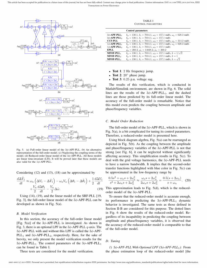
Fig. 5. (a) Full-order linear model of the 3φ-APF-PLL. (b) An alternativerepresentation of the full-order model. (c) Neglecting the coupling terms of themodel. (d) Reduced-order linear model of the 3φ-APF-PLL. All these modelsare linear time-invariant (LTI). It will be proved later that these models arealso valid for the 1φ-APF-PLL.

Considering (12) and (13), (18) can be approximated by

d∆V1

dt≈ ωn

(∆V1 −∆V1

)− ωnVn

(∆θ1 −∆θ1

)+

1

2

d∆V1

dt

+Vn2

d∆θ1

dt− Vn

2∆ω. (19)

Using (14), (19), and the linear model of the SRF-PLL [19,Fig. 3], the full-order linear model of the 3φ-APF-PLL can bedeveloped as shown in Fig. 5(a).

B. Model Verification

In this section, the accuracy of the full-order linear model[Fig. 5(a)] of the 3φ-APF-PLL is investigated. As shown inFig. 3, there is an optional LPF in the 3φ-APF-PLL q-axis. The3φ-APF-PLL with and without this LPF is called the 3φ-APF-PLL1 and 3φ-APF-PLL2, respectively. Here, for the sake ofbrevity, we only present the model verification results for the3φ-APF-PLL1. The control parameters of the 3φ-APF-PLL1

can be found in Table I.Three tests are considered for the model verification.

TABLE ICONTROL PARAMETERS

Control parameters

3φ-APF-PLL1 kp = 130.1, ki = 7014.1, ωd = 157.1 rad/s, ωq = 628.3 rad/s3φ-APF-PLL2 kp = 130.1, ki = 7014.1, ωd = 157.1 rad/sCCF-PLL kp = 130.1, ki = 7014.1, ωd = 157.1 rad/s, ωp = 314.2 rad/s1φ-APF-PLL1 kp = 130.1, ki = 7014.1, ωd = 157.1 rad/s, ωq = 628.3 rad/s1φ-APF-PLL2 kp = 130.1, ki = 7014.1, ωd = 157.1 rad/sEPLL µp = 260.2, µi = 14028.2, µv = 260.2

MFOF-PLL1 kp = 130.1, ki = 7014.1, ωd = 157.1 rad/s, k = 1/√

2MFOF-PLL2 kp = 130.1, ki = 7014.1, ωd = 157.1 rad/s, k = 1

MFOF-PLL3 kp = 130.1, ki = 7014.1, ωd = 157.1 rad/s, k =√

2

• Test 1: 2 Hz frequency jump.• Test 2: 20◦ phase jump.• Test 3: 0.25 p.u. voltage sag.

The results of this verification, which is conducted inMatlab/Simulink environment, are shown in Fig. 6. The solidlines are the results of the 3φ-APF-PLL1, and the dashedlines are those predicted by its full-order linear model. Theaccuracy of the full-order model is remarkable. Notice thatthis model even predicts the coupling between amplitude andphase/frequency variables.

C. Model Order Reduction

The full-order model of the 3φ-APF-PLL, which is shown inFig. 5(a), is a bit complicated for tuning its control parameters.Therefore, a reduced-order model is presented here.

Using block diagram algebra, Fig. 5(a) can be rearranged asdepicted in Fig. 5(b). As the coupling between the amplitudeand phase/frequency variables of the 3φ-APF-PLL is not thatstrong [see Fig. 6], it can be neglected without significantlyaffecting accuracy. This simplification results in Fig. 5(c). Todeal with the grid voltage harmonics, the 3φ-APF-PLL needsto have a narrow bandwidth. It implies that the second-ordertransfer functions highlighted with blue color in Fig. 5(c) canbe approximated in the low-frequency range by

0.5s2 + ωns+ 2ω2n

s2 + 2ωns+ 2ω2n

≈ ωns+ 2ω2n

2ωns+ 2ω2n

=0.5(s+ 2ωn)

s+ ωn. (20)

This approximation leads to Fig. 5(d), which is the reduced-order model of the 3φ-APF-PLL.

To ensure that the reduced-order model is accurate enough,its performance in predicting the 3φ-APF-PLL1 dynamicbehavior is investigated. The same tests as those defined inSection II-B are considered for this purpose. The dotted linesin Fig. 6 show the results of the reduced-order model. Re-gardless of its incapability in predicting the coupling betweenamplitude and phase/frequency variables, it is observed thatthe accuracy of the reduced-order model is comparable to thatof the full-order model.

D. Tuning

1) 3φ-APF-PLL With Optional LPF (3φ-APF-PLL1): Fromthe phase estimation loop of the reduced-order model [the



0 0.02 0.04 0.06 0.08 0.1-1

-0.5

0

0.5

1G

rid v

olt

age

(p.u

.)

0 0.02 0.04 0.06 0.08 0.149.5

50

50.5

51

51.5

52

52.5

Est

imat

ed f

requen

cy (

Hz)

3?-APF-PLL1 [Fig.3]Full-order model [Fig. 5(a)] Reduced-order model [Fig. 5(d)]

0 0.02 0.04 0.06 0.08 0.1-1

0

1

2

3

4

5

Phas

e er

ror

(deg

) 3?-APF-PLL1 [Fig.3]Full-order model [Fig. 5(a)] Reduced-order model [Fig. 5(d)]

0 0.02 0.04 0.06 0.08 0.10.995

1

1.005

Time (s)

Est

imat

ed a

mpli

tude

(p.u

.)


(a)

0 0.02 0.04 0.06 0.08 0.1-1

-0.5

0

0.5

1

Gri

d v

olt

age

(p.u

.)

0 0.02 0.04 0.06 0.08 0.149

50

51

52

53

Est

imat

ed f

requen

cy (

Hz)


0 0.02 0.04 0.06 0.08 0.1-10

0

10

20

Phas

e er

ror

(deg

) 3?-APF-PLL1 [Fig.3]Full-order model [Fig. 5(a)] Reduced-order model [Fig. 5(d)]

0 0.02 0.04 0.06 0.08 0.10.96

0.98

1

1.02

1.04

Time (s)

Est

imat

ed a

mpli

tude

(p.u

.)


(b)

0 0.02 0.04 0.06 0.08 0.1-1

-0.5

0

0.5

1

Gri

d v

olt

age

(p.u

.)

0 0.02 0.04 0.06 0.08 0.1

49.9

49.95

50

50.05

50.150.1

Est

imat

ed f

requen

cy (

Hz)


0 0.02 0.04 0.06 0.08 0.1-1

-0.5

0

0.5

Phas

e er

ror

(deg

)


0 0.02 0.04 0.06 0.08 0.10.7

0.75

0.8

0.85

0.9

0.95

1

1.05

Time (s)

Est

imat

ed a

mpli

tude

(p.u

.)


(c)

Fig. 6. 3φ-APF-PLL1 model verification. (a) Test 1: 2-Hz frequency jump. (b) Test 2: 20◦ phase jump. (c) Test 3: 0.25-p.u. voltage sag. The estimatedfrequency and amplitude by the 3φ-APF-PLL1 denote the signals ω and V1 in Fig. 3, and the phase error is the difference of the actual and estimated phaseangles. The estimated frequency, estimated amplitude, and phase error in the full-order and reduced-order models are the signals ∆ω + ωn, ∆V1 + Vn, and∆θ1 − ∆θ1, respectively. The control parameters of the 3φ-APF-PLL1 can be found in Table I. The sampling frequency and the grid nominal frequencythroughout this paper are 10 kHz and 50 Hz, respectively.

lower part of Fig. 5(d)], the following open-loop transferfunction can be obtained:

G3φ−APF−PLL1

ol (s)=∆θ1(s)

∆θ1(s)−∆θ1(s)

= Vn0.5 (s+ 2ωn)

s+ ωn

ωqs+ ωq

kps+ kis2

. (21)

It is observed that selecting ωq = 2ωn = 628.3 rad/s resultsin a pole-zero cancellation and simplifies (21) as

G3φ−APF−PLL1

ol (s) = Vnωn

s+ ωn

kps+ kis2

. (22)

The open-loop transfer function (22) describes a type-2control system (i.e., a system with two open-loop poles atthe origin) with a pole-zero pair. For such a system, thesymmetrical optimum method (SOM)4 is a good option for thetuning procedure [19], [20]. Notice that the open-loop pole in(22) is already fixed. Therefore, using the SOM results in

kp =ωcVn

=ωnVnb

(23a)

ki =ω2c

Vnb=

ω2n

Vnb3(23b)

where the design constant b determines the PM value. Byconsidering PM= π/4 rad (45◦), which is recommended in[19], b = 1+

√2 is achieved. Substituting this value into (23),

4The SOM sets the crossover frequency at the geometric mean of the pole-zero pair (i.e., ωc =

√ωnki/kp) to maximize the phase margin (PM) [19],

[20]. The ratio of the pole-zero pair, i.e., b2 = ωnki/kp

, then determines the

PM value as PM = tan−1(

b2−12b

).

gives kp = 130.1 and ki = 7014.1.

The remaining design parameter is the cutoff-frequencyωd, which regulates the 3φ-APF-PLL1 amplitude estimationdynamics. A high value for this parameter makes the dynamicresponse of the amplitude estimation faster, but at the cost ofreducing the noise immunity. Therefore, one has to make atrade-off decision. Here, based on a trial-and-error procedure,ωd = wn/2 = 157.1 rad/s is selected.

2) 3φ-APF-PLL Without Optional LPF (3φ-APF-PLL2):By neglecting the optional LPF in Fig. 5(d), the open-looptransfer function of the 3φ-APF-PLL2 can be obtained as

G3φ−APF−PLL2

ol (s)=∆θ1(s)

∆θ1(s)−∆θ1(s)

= Vn0.5 (s+ 2ωn)

s+ ωn

kps+ kis2

. (24)

The highlighted fraction on the right hand side of (24) isa lag filter, which models the APF dynamics. In the low-frequencies range (i.e., in frequencies less than the fundamen-tal frequency), this term can be neglected without significantlyaffecting the accuracy. Therefore, in the same range, theclosed-loop transfer function of the 3φ-APF-PLL2 can beapproximated by

G3φ−APF−PLL2

cl (s) =∆θ1(s)

∆θ1(s)≈ Vnkps+ Vnkis2 + Vnkps+ Vnki

. (25)

Using (22), the closed-loop transfer function of 3φ-APF-PLL1 may also be approximated in the low-frequency range



(a)

(b)

, 1v

1s1

s

iks

pk

ˆ

1

1nVp

ps

1V 1Vd

dsp

ps

SRF-PLLCCF-based sequence detector

dq dv

qv

p

p 1s

1s

v

v

p

p 1s

1s

v

v

abc

av

bv

cvn

sincos

iks

pk

1s

ˆ

1V

1

d

ds1v

1v

1v

1v

, 1v

, 1v

, 1v

1

Fig. 7. (a) Block diagram of the CCF-PLL. (b) Small-signal model of theCCF-PLL.

by

G3φ−APF−PLL1

cl (s) =∆θ1(s)

∆θ1(s)

=ωn(Vnkps+ Vnki)

s3 + ωns2 + Vnωnkps+ Vnωnki

≈ ωn(Vnkps+ Vnki)

ωns2 + Vnωnkps+ Vnωnki=

Vnkps+ Vnkis2 + Vnkps+ Vnki

. (26)

A comparison of (25) and (26) suggests that to have a faircomparison, kp and ki of the 3φ-APF-PLL2 should be selectedthe same as those of the 3φ-APF-PLL1. The same goes forthe LPF cutoff frequency ωd (see Table I).

E. Performance Assessment

In this section, a comparison among the 3φ-APF-PLL1,3φ-APF-PLL2, and a complex-coefficient filter (CCF) basedPLL (CCF-PLL) [21] [see Fig. 7(a)] is conducted. The CCF-PLL includes two complex band-pass filters with the centerfrequency at the fundamental positive-sequence and negative-sequence frequencies. These band-pass filters work collabo-ratively and extract the fundamental positive- and negative-sequence components of the grid voltage. The extracted FFPScomponent is fed to the SRF-PLL, which extracts the phase,frequency, and amplitude of this component. The estimatedfrequency is fed back to the complex filters to adapt them togrid frequency changes.

The small-signal model of the CCF-PLL can be observedin Fig. 7(b) [19], [22].5 From the this model, the open-looptransfer function (27) can be obtained.

GCCF−PLLol (s) =

∆θ1(s)

∆θ1(s)−∆θ1(s)= Vn

ωps+ ωp

kps+ kis2

.

(27)

5It is the most accurate available model for the CCF-PLL. In obtaining thismodel, the dynamics of the CCF tuned at the fundamental frequency of thenegative sequence has been neglected.

TABLE IISTABILITY MARGINS OF 3φ-APF-PLL1 , 3φ-APF-PLL2 , AND CCF-PLL

AND DETAILS OF THEIR NUMERICAL COMPARISON

3φ-APF-PLL1 3φ-APF-PLL2 CCF-PLL

Test A: DC offsetPeak-to-peak frequency error 0.41 Hz 0.41 Hz 0.67 HzPeak-to-peak phase error 2.76◦ 2.75◦ 4.51◦

Peak-to-peak amplitude error 0.04 p.u. 0.04 p.u. 0.07 p.u.Test B: Imbalance and harmonicsPeak-to-peak frequency error 0.02 Hz 0.08 Hz 0.02 HzPeak-to-peak phase error 0.15◦ 0.56◦ 0.13◦

Peak-to-peak amplitude error 0.01 p.u. 0.01 p.u. 0 p.u.Test C: Phase jump2% settling time 47.3 ms 54.6 ms 48.5 msPhase overshoot 34.73% 24.01% 39.52%Peak frequency variation 2.52 Hz 2.24 Hz 2.68 HzPeak amplitude variation 0.04 p.u. 0.03 p.u. 0.06 p.u.Test D: Frequency jump2% settling time 37.4 ms 40.5 ms 37.5 msFrequency overshoot 1.09% 1.74% 0.62%Peak phase variation 4.9◦ 4.24◦ 5.09◦

Peak amplitude variation 0 p.u. 0 p.u. 0.01 p.u.Phase margin 43.5◦ 55.7◦ 45◦

Note: All results are rounded to 2 decimal places.

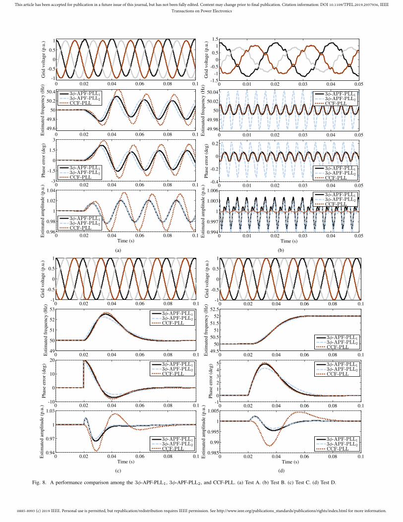
Based on (22) and (27), it is immediate to conclude thatto have a fair performance comparison, the proportional andintegral gains of the CCF-PLL should be the same as thoseof the 3φ-APF-PLL1, and the CBF gain ωp should be equalto ωn. Table I summarizes the control parameters of the 3φ-APF-PLL1, 3φ-APF-PLL2, and CCF-PLL.

Four tests are considered.• In Test A, a 0.1 p.u. dc component is added to the phaseA of the grid voltage.

• In Test B, the grid voltage is imbalanced and distortedwith characteristic harmonics of order −5, +7, −11, and+13. The magnitude of all harmonics is 5%.

• In Test C, a 20◦ phase jump in the grid voltage happens.• In Test D, the grid voltage experiences a 2-Hz frequency

jump.Fig. 8 shows the results of these tests, and Table II sum-

marizes their details. According to these results, the followingobservations can be made:• The 3φ-APF-PLL1 and 3φ-APF-PLL2 offer a higher dc-

offset filtering capability than the CCF-PLL.• The CCF-PLL and 3φ-APF-PLL2 offer the best and

worst harmonic filtering capabilities, respectively. Theharmonic rejection ability of the 3φ-APF-PLL1 is closeto that of the CCF-PLL. Notice that all these PLLscompletely reject the grid voltage imbalance.

• In estimating the phase and frequency variables, the3φ-APF-PLL2 offers a more damped dynamic responsecompared to the CCF-PLL and 3φ-APF-PLL1, which isattributable to its higher phase margin [see Fig. 9].

• The estimated amplitude of the CCF-PLL experienceslarger transients when phase and frequency jumps hap-pen. It means that the coupling between the amplitudeand phase/frequency variables in the CCF-PLL is strongerthan that in the 3φ-APF-PLL1 and 3φ-APF-PLL2.

To confirm the above simulation results, Test A is repeatedexperimentally using the dSPACE 1006 platform. To this end,the mains voltage [which is a 50 Hz/230-V (phase RMS)



0 0.02 0.04 0.06 0.08 0.1-1

-0.5

0

0.5

1G

rid v

olt

age

(p.u

.)

0 0.02 0.04 0.06 0.08 0.1

49.6

49.8

50

50.2

50.4

Est

imat

ed f

requen

cy (

Hz)

3?-APF-PLL1

3?-APF-PLL2

CCF-PLL

0 0.02 0.04 0.06 0.08 0.1-3

-1.5

0

1.5

3

Phas

e er

ror

(deg

)

3?-APF-PLL1

3?-APF-PLL2

CCF-PLL

0 0.02 0.04 0.06 0.08 0.10.96

0.98

1

1.02

1.04

Time (s)

Est

imat

ed a

mpli

tude

(p.u

.)

3?-APF-PLL1

3?-APF-PLL2

CCF-PLL

(a)

0 0.01 0.02 0.03 0.04 0.05-1.5

-1

-0.5

0

0.5

1

1.5

Gri

d v

olt

age

(p.u

.)

0 0.01 0.02 0.03 0.04 0.05

49.96

49.98

50

50.02

50.04

Est

imat

ed f

requen

cy (

Hz)

3?-APF-PLL1

3?-APF-PLL2

CCF-PLL

0 0.01 0.02 0.03 0.04 0.05-0.4

-0.2

0

0.2

Phas

e er

ror

(deg

)

3?-APF-PLL1

3?-APF-PLL2

CCF-PLL

0 0.01 0.02 0.03 0.04 0.050.994

0.997

1

1.003

1.006

Time (s)

Est

imat

ed a

mpli

tude

(p.u

.)

3?-APF-PLL1

3?-APF-PLL2

CCF-PLL

(b)

0 0.02 0.04 0.06 0.08 0.1-1

-0.5

0

0.5

1

Gri

d v

olt

age

(p.u

.)

0 0.02 0.04 0.06 0.08 0.149

50

51

52

53

Est

imat

ed f

requen

cy (

Hz)

3?-APF-PLL1

3?-APF-PLL2

CCF-PLL

0 0.02 0.04 0.06 0.08 0.1-10

0

10

20

Phas

e er

ror

(deg

) 3?-APF-PLL1

3?-APF-PLL2

CCF-PLL

0 0.02 0.04 0.06 0.08 0.10.94

0.97

1

1.03

Time (s)

Est

imat

ed a

mpli

tude

(p.u

.)

3?-APF-PLL1

3?-APF-PLL2

CCF-PLL

(c)

0 0.02 0.04 0.06 0.08 0.1-1

-0.5

0

0.5

1

Gri

d v

olt

age

(p.u

.)

0 0.02 0.04 0.06 0.08 0.149.5

50

50.5

51

51.5

52

52.5

Est

imat

ed f

requen

cy (

Hz)

3?-APF-PLL1

3?-APF-PLL2

CCF-PLL

0 0.02 0.04 0.06 0.08 0.1-1

0

1

2

3

4

5

Phas

e er

ror

(deg

) 3?-APF-PLL1

3?-APF-PLL2

CCF-PLL

0 0.02 0.04 0.06 0.08 0.10.985

0.99

0.995

1

1.005

Time (s)

Est

imat

ed a

mpli

tude

(p.u

.)

3?-APF-PLL1

3?-APF-PLL2

CCF-PLL

(d)

Fig. 8. A performance comparison among the 3φ-APF-PLL1, 3φ-APF-PLL2, and CCF-PLL. (a) Test A. (b) Test B. (c) Test C. (d) Test D.



-40

-20

0

20

40

60M

agnit

ude

(dB

)

100

101

102

103

-180

-150

-120

Phas

e (d

eg)

Frequency (Hz)

3?-APF-PLL1

3?-APF-PLL2

CCF-PLL

3?-APF-PLL1

3?-APF-PLL2

CCF-PLL

-60-90

5 7

45 3.

Fig. 9. Open-loop Bode plots of the 3φ-APF-PLL1, 3φ-APF-PLL2, andCCF-PLL. These plots are obtained using linear models shown in Fig. 5(c)and 7(b).

Gri

d v

olt

age

(p.u

.)

0

0.5

1.5

1

2

-0.5

-1

-1.510 ms

10 ms

3ϕ-APF-PLL2

CCF-PLL

3ϕ-APF-PLL1

Est

imat

ed f

requ

ency

(H

z)

50.2

50.4

49.8

50

50.6

50.8

49.649.4

Fig. 10. Experimental performance comparison of the 3φ-APF-PLL1, 3φ-APF-PLL2, and CCF-PLL in response to Test A (adding 0.1 p.u. dc compo-nent to phase A).

system] is measured using a sensor board and fed to theDS2004 A/D board. The digital grid voltage signals are thennormalized by dividing them by the nominal amplitude. A0.1 p.u. dc component is then generated in the real-time codeand added to the phase A. The responses of PLLs to thisdisturbance are sent out using DS2102 DAC board and shownon a digital oscilloscope [Tektronix DPO 2014B]. The resultsof this experimental test can be observed in Fig. 10. To savespace, only the estimated frequencies by the PLLs are shown.As shown, these results are the same as simulation one [seeFig. 8(a)].

dqn

qv

dv

sincos

iks

pk

1s

Optional LPF

1V

1

d

ds

q

qs

v2v

0

APF

APFv 0.5

0.5 v

v

1v

1v

SRF‐PLLAPF‐based FFPS

component detector

Fig. 11. Alternative mathematically-equivalent representation of the 1φ-APF-PLL.

III. 1φ-APF-PLL

A. Modeling

From Fig. 1, an alternative representation of the 1φ-APF-PLL can be obtained as shown in Fig. 11. This representationdemonstrates that the 1φ-APF-PLL is actually a special caseof the 3φ-APF-PLL where its β-axis input is equal to zero.By assuming that the single-phase grid voltage signal v isas (28), where V1 and θ1 are the amplitude and phase angle,respectively, the signals vα and vβ in Fig. 11 can be expressedas (29).

v(t) = V1 cos(θ1) (28)

vα(t) = 2v(t) =

FFPSCom.︷︸︸︷V1 cos(θ1) +

FFNSCom.︷︸︸︷V1 cos(−θ1)

vβ(t) = 0 = V1 sin (θ1) + V1 sin(−θ1)

(29)

In (29), FFPS Com. and FFNS Com. denote the fundamental-frequency positive-sequence and negative-sequence compo-nents, respectively.

The equation (29) describes a set of imbalanced signals inthe αβ frame, where its positive and negative sequence compo-nents have the same amplitude. Fortunately, the FFNS compo-nent is blocked in the steady state because the transfer functionbetween the vectors vα(s) + jvβ(s) and vα1(s) + jvβ1(s) inFig. 11 has a zero magnitude at the fundamental negativefrequency [see Fig. 4]. Therefore, the FFNS component can beneglected during the modeling procedure without significantlyaffecting the accuracy. Considering this fact and the similarityof Fig. 3 and 11, it can be concluded that the LTI models of3φ-APF-PLL [see Fig. 5] are also valid for the 1φ-APF-PLL.

B. Model Verification

In this section, the accuracy of the full-order and reduced-order models of the 1φ-APF-PLL is investigated. As men-tioned before, the 1φ-APF-PLL has an optional LPF in its q-axis [see Fig. 1]. The 1φ-APF-PLL with and without this LPFis called the 1φ-APF-PLL1 and 1φ-APF-PLL2, respectively.To save space, the model verification of the 1φ-APF-PLL1 isonly presented here.

Fig. 12 shows the model verification results. It is observedthat both models precisely predict the dynamics of phaseand frequency variables in Test 1 and 2 (i.e., the phase andfrequency jump tests), and accurately anticipate the amplitudeestimation dynamics in Test 3 (the voltage sag test). They,however, fail to do so in predicting the coupling betweenamplitude and phase/frequency variables. In the case of the



0 0.02 0.04 0.06 0.08 0.1-1

-0.5

0

0.5

1G

rid v

olt

age

(p.u

.)

0 0.02 0.04 0.06 0.08 0.149.5

50

50.5

51

51.5

52

52.5

Est

imat

ed f

requen

cy (

Hz)

1?-APF-PLL1 [Fig.1]Full-order model [Fig. 5(a)]Reduced-order model [Fig. 5(d)]

0 0.02 0.04 0.06 0.08 0.1-1

0

1

2

3

4

5

Phas

e er

ror

(deg

) 1?-APF-PLL1 [Fig.1]Full-order model [Fig. 5(a)]Reduced-order model [Fig. 5(d)]

0 0.02 0.04 0.06 0.08 0.10.994

0.997

1

1.003

1.006

Time (s)

Est

imat

ed a

mpli

tude

(p.u

.)


(a)

0 0.02 0.04 0.06 0.08 0.1-1

-0.5

0

0.5

1

Gri

d v

olt

age

(p.u

.)

0 0.02 0.04 0.06 0.08 0.1

50

51

52

53

Est

imat

ed f

requen

cy (

Hz)


0 0.02 0.04 0.06 0.08 0.1-10

0

10

20

Phas

e er

ror

(deg

) 1?-APF-PLL1 [Fig.1]Full-order model [Fig. 5(a)]Reduced-order model [Fig. 5(d)]

0 0.02 0.04 0.06 0.08 0.10.91

0.94

0.97

1

1.03

Time (s)

Est

imat

ed a

mpli

tude

(p.u

.)


(b)

0 0.02 0.04 0.06 0.08 0.1-1

-0.5

0

0.5

1

Gri

d v

olt

age

(p.u

.)

0 0.02 0.04 0.06 0.08 0.149.8

50

50.2

50.4

Est

imat

ed f

requen

cy (

Hz)


0 0.02 0.04 0.06 0.08 0.1-4

-3

-2

-1

0

1

Phas

e er

ror

(deg

)


0 0.02 0.04 0.06 0.08 0.10.7

0.75

0.8

0.85

0.9

0.95

1

1.05

Time (s)

Est

imat

ed a

mpli

tude

(p.u

.)


(c)

Fig. 12. 1φ-APF-PLL1 model verification. (a) Test 1: 2-Hz frequency jump. (b) Test 2: 20◦ phase jump. (c) Test 3: 0.25 p.u. voltage sag. The controlparameters of the 1φ-APF-PLL1 can be found in Table I.

reduced-order model, this result was expected because it isobtained by neglecting the coupling terms in the full-ordermodel. In the case of the full-order model, however, thisinaccuracy requires justification, which is explained in whatfollows.

During the modeling of the 1φ-APF-PLL in Section III-A,the FFNS component highlighted in (29) was neglected. Noticethat occurring a disturbance (for example, a phase, a frequency,or an amplitude jump) results in a change in this FFNScomponent, which affects the 1φ-APF-PLL transient response.The full-order model, however, does not consider this com-ponent and, therefore, cannot predict its effects. It is worthmentioning here that considering the FFNS component duringthe modeling procedure results in a linear-time periodic (LTP)model, which is more complicated to analyze compared to LTImodels developed in this paper. For more details about the LTPmodeling of single-phase grid synchronization systems, referto [23].

C. Performance Comparison

In this section, a comparison among the 1φ-APF-PLL1,1φ-APF-PLL2 and enhanced PLL (EPLL) [5], [24], whichis a well-known single-phase PLL, is conducted. The blockdiagram of the EPLL and its linear model may be observedin Fig. 13.

Equation (30) is the EPLL closed-loop transfer function,which can be obtained from its LTI model.

GEPLLcl (s) =

∆θ1(s)

∆θ1(s)=

0.5Vn(µps+ µi)

s2 + 0.5Vnµps+ 0.5Vnµi(30)

(a)

(b)

cos

n

-sin

v

ˆ

1sv

1

1V

1s1

s

ˆ

1

1 /2nV

1s1 / 21V

1V

i

s

v

s

i

s

p

p

v

Fig. 13. (a) Block diagram representation of the EPLL. (b) EPLL LTI model.µp, µi, and µv are the EPLL control parameters.

If we compare the above transfer function with (25) or (26),6 itcan be concluded that a fair comparison between the EPLL and1φ-APF-PLL1/1φ-APF-PLL2 demands µp = 2kp and µi =2ki. Table I summarizes the control parameters of all thesePLLs.

Four numerical tests are conducted.

6The equations (25) or (26) are the (approximate) closed-loop transferfunctions of the 3φ-APF-PLL2 and 3φ-APF-PLL1, respectively, which areobtained from their reduced-order LTI model [see Fig. 5(d)]. As the 1φ-APF-PLL and 3φ-APF-PLL have the same models, it can be concluded that thesetransfer functions are valid for the 1φ-APF-PLL2 and 1φ-APF-PLL1 too.



0 0.02 0.04 0.06 0.08 0.1-1

-0.5

0

0.5

1G

rid v

olt

age

(p.u

.)

0 0.02 0.04 0.06 0.08 0.149.5

50

50.5

Est

imat

ed f

requen

cy (

Hz)

1?-APF-PLL1

1?-APF-PLL2

EPLL

0 0.02 0.04 0.06 0.08 0.1-4

-2

0

2

4

Phas

e er

ror

(deg

)

1?-APF-PLL1

1?-APF-PLL2

EPLL

0 0.02 0.04 0.06 0.08 0.10.94

0.97

1

1.03

1.06

Time (s)

Est

imat

ed a

mpli

tude

(p.u

.)

1?-APF-PLL1

1?-APF-PLL2

EPLL

(a)

0 0.02 0.04 0.06 0.08 0.1-1

-0.5

0

0.5

1

Gri

d v

olt

age

(p.u

.)

0 0.02 0.04 0.06 0.08 0.149.8

49.9

50

50.1

50.2

Est

imat

ed f

requen

cy (

Hz)

1?-APF-PLL1

1?-APF-PLL2

EPLL

0 0.02 0.04 0.06 0.08 0.1-1.5

-0.75

0

0.75

1.5

Phas

e er

ror

(deg

)

1?-APF-PLL1

1?-APF-PLL2

EPLL

0 0.02 0.04 0.06 0.08 0.10.97

0.985

1

1.015

1.031.03

Time (s)

Est

imat

ed a

mpli

tude

(p.u

.)

1?-APF-PLL1

1?-APF-PLL2

EPLL

(b)

0 0.02 0.04 0.06 0.08 0.1-1

-0.5

0

0.5

1

Gri

d v

olt

age

(p.u

.)

0 0.02 0.04 0.06 0.08 0.149

50

51

52

53

Est

imat

ed f

requen

cy (

Hz)

1?-APF-PLL1

1?-APF-PLL2

EPLL

0 0.02 0.04 0.06 0.08 0.1-10

0

10

20

Phas

e er

ror

(deg

) 1?-APF-PLL1

1?-APF-PLL2

EPLL

0 0.02 0.04 0.06 0.08 0.10.85

0.9

0.95

1

1.05

Time (s)

Est

imat

ed a

mpli

tude

(p.u

.)

1?-APF-PLL1

1?-APF-PLL2

EPLL

(c)

0 0.02 0.04 0.06 0.08 0.1-1

-0.5

0

0.5

1

Gri

d v

olt

age

(p.u

.)

0 0.02 0.04 0.06 0.08 0.149.5

50

50.5

51

51.5

52

52.5

Est

imat

ed f

requen

cy (

Hz)

1?-APF-PLL1

1?-APF-PLL2

EPLL

0 0.02 0.04 0.06 0.08 0.1-1

0

1

2

3

4

5

Phas

e er

ror

(deg

) 1?-APF-PLL1

1?-APF-PLL2

EPLL

0 0.02 0.04 0.06 0.08 0.10.97

0.98

0.99

1

1.01

Time (s)

Est

imat

ed a

mpli

tude

(p.u

.)

1?-APF-PLL1

1?-APF-PLL2

EPLL

(d)

Fig. 14. A performance comparison among the 1φ-APF-PLL1, 1φ-APF-PLL2, and EPLL. (a) Test A∗. (b) Test B∗. (c) Test C∗. (d) Test D∗.



TABLE IIISTABILITY MARGINS OF 1φ-APF-PLL1 , 1φ-APF-PLL2 , AND EPLL AND

DETAILS OF THEIR NUMERICAL COMPARISON

1φ-APF-PLL1 1φ-APF-PLL2 EPLL

Test A∗: DC offsetPeak-to-peak frequency error 0.75 Hz 0.71 Hz 0.79 HzPeak-to-peak phase error 5.02◦ 4.79◦ 5.37◦

Peak-to-peak amplitude error 0.07 p.u. 0.08 p.u. 0.09 p.u.Test B∗: HarmonicsPeak-to-peak frequency error 0.12 Hz 0.18 Hz 0.26 HzPeak-to-peak phase error 0.8◦ 1.2◦ 1.74◦

Peak-to-peak amplitude error 0.04 p.u. 0.04 p.u. 0.03 p.u.Test C∗: Phase jump2% settling time 48.1 ms 54.6 ms 56 msPhase overshoot 34.06% 24.31% 24.65%Peak frequency variation 2.66 Hz 2.39 Hz 2.12 HzPeak amplitude variation 0.09 p.u. 0.08 p.u. 0.12 p.u.Test D∗: Frequency jump2% settling time 38.4 ms 40.7 ms 43.1 msFrequency overshoot 1.06% 1.64% 2.07%Peak phase variation 4.66◦ 4.16◦ 4.57◦

Peak amplitude variation 0.01 p.u. 0.01 p.u. 0.02 p.u.Phase margin 43.5◦ 55.7◦ 68.9◦


• In Test A∗, a 0.05 p.u. dc component is suddenly addedto the PLLs input signal.

• In Test B∗, the input signal is contaminated with low-order harmonics of order 3, 5, 7, and 9. The amplitudes ofthese harmonics are 5%, 4%, 3%, and 2%, respectively,which are corresponding to a total harmonic distortionaround 7.35%.

• In Test C∗, a 20◦ phase jump in the PLLs input signalhappens.

• In Test D∗, a 2-Hz frequency jump in the PLLs inputsignal occurs.

The results of these tests and their details can be foundin Fig. 14 and Table III, respectively. From these results, thefollowing observations are made.• All PLLs demonstrate a close level of dc-offset filtering

capability.• The 1φ-APF-PLL1, thanks to its in-loop LPF, represents

a slightly better performance than the 1φ-APF-PLL2 andEPLL in filtering harmonics.

• The 1φ-APF-PLL1 demonstrates a larger phase overshootthan the 1φ-APF-PLL2 and EPLL after the phase jump.The main reason behind this observation is the phasedelay caused by its in-loop LPF, which reduces its phasemargin. This fact is clear from Fig. 15.

• There is not a large difference between the settlingtime of 1φ-APF-PLL1, 1φ-APF-PLL2, and EPLL duringtransients.

IV. MFOF-PLLA. Description and Modeling

The MFOF, which is used for generating the fictitiousquadrature signal in the MFOF-PLL [see Fig. 2], is expressedin the Laplace domain as [15]

GMFOF(s) =ω − kss+ kω

(31)

-40

-20

0

20

40

60

Mag

nit

ude

(dB

)

)100

101

102 3

-180

-135

Phas

e (d

eg)

1?-APF-PLL1

1?-APF-PLL2

EPLL

1?-APF-PLL1

1?-APF-PLL2

EPLL-60-90

5 7

3.

Frequency (Hz)10

Fig. 15. Open-loop Bode plots of the 1φ-APF-PLL1, 1φ-APF-PLL2, andEPLL. These plots are obtained using the linear models shown in Fig. 5(c)and 13(b).

where k is the design constant of this filter, and ω is the gridvoltage angular frequency. Notice that, as shown in Fig. 2, theestimated frequency is fed back to the MFOF to adapt it tofrequency variations.

Fig. 16 shows the MFOF frequency response for threedifferent values of k. From this plot and the transfer function(31), the following observations are made:

• Regardless of the value of k, the MFOF has −90◦ phaseat the fundamental frequency.

• k = 1 results in a unity amplitude at all frequencies andtherefore make the MFOF a first-order APF.

• 0 ≤ k < 1 amplifies the dc component and sub-harmonics and attenuates frequencies larger than thefundamental frequency. Notice that k = 0 makes theMFOF an ideal integrator.

• k > 1 attenuates the dc component and sub-harmonicsand amplifies frequencies larger than the fundamentalfrequency. Notice that k = ∞ makes the MFOF adifferentiator.

Fig. 17 illustrates an alternative mathematically-equivalentrepresentation of the MFOF-PLL. Considering this structure,the discussions conducted in Section III-A, and the mathemat-ical modeling procedure presented in Section II-A, the full-order model of the MFOF-PLL can be obtained as shownin Fig. 18(a). By applying the block diagram algebra, thismodel can be rearranged as Fig. 18(b). Neglecting the cross-coupling terms leads to Fig. 18(c). Further simplification canbe achieved by replacing the second-order transfer functionsin Fig. 18(c) by their first-order approximations, as depicted inFig. 18(d). These models are useful for measuring the stabilitymargin of the MFOF-PLL, tuning its control parameters, andanalyzing its performance. The accuracy of these models canbe verified using numerical results. To save space, the modelverification results are not presented here.



-4

-2

0

2

4

Mag

nit

ude

(dB

)

100

101

102

103

-180

-135

-90

-45

0

Phas

e (d

eg)

Frequency (Hz)

MFOF (k = 1/√

2) MFOF (k = 1) MFOF (k =√

2)

Fig. 16. Frequency response of the MFOF for three different values of k.

dqn

qv

dv

sincos

iks

pk

1s

Optional LPF

1V

1

d

ds

q

qs

v2v

0MFOFv 0.5

0.5 v

v

1v

1v

SRF‐PLLMFOF‐based FFPS

component detector

MFOF

Fig. 17. Alternative mathematically-equivalent representation of the MFOF-PLL.

B. Performance Assessment

As discussed before, the only difference of the MFOF-PLL compared to the 1φ-APF-PLL is the additional degree offreedom k in its structure [see Figs. 1 and 2]. This section aimsto investigate the effects of this additional degree of freedom.To this end, the following cases are considered:

• MFOF-PLL1: k = 1/√

2• MFOF-PLL2: k = 1• MFOF-PLL3: k =

√2.

In all these cases, the optional LPF in the q-axis is neglected.Notice that, as mentioned before, k = 1 makes the MFOF afirst-order APF. Therefore, the MFOF-PLL2 and the 1φ-APF-PLL2 are the same systems. Considering this fact, the controlparameters of the MFOF-PLL2 are selected the same as thoseof the 1φ-APF-PLL2 [see Table I]. As the objective here isto investigate the effects of the parameter k, the proportionaland integral gains of the MFOF-PLL1 and MFOF-PLL3 andthe cutoff frequency of their d-axis LPF are chosen the sameas those of the MFOF-PLL2.

The same tests as those defined in Section III-C are con-sidered for the investigation here. Fig. 19 shows the results ofthese tests, and Table IV summarizes the details of the results.From these results, the following observations are made:

• MFOF-PLL1 and MFOF-PLL3, which have the lowestand highest value of k, have the worst and best dc-offset

(a)

(b)

(c)

(d)

SRF-PLL

1s

0.5

1s

0.5

0.5

1s

1s

iks

pk

1

1

1V1

V

1

1V

d

ds

nVn

k

nk

1/ nkV

/nV k

nkV

nkV

/ nk V

Optional LPF

q

qs

iks

pk 1s

1s

1

1

1V1

V d

ds

nV

2 2 2

2 2 2

0.5 ( 1)

2 ( 1)n n

n n

s k s k

s k s k

2 2 2

2 2 2

0.5 ( 1)

2 ( 1)n n

n n

s k s k

s k s k

Optional LPF

q

qs

1s

1

1V

1Vd

ds

nV

2 2 2

2 2 2

0.5 ( 1)

2 ( 1)n n

n n

s k s k

s k s k

2 2 2

2 2 2

0.5 ( 1)

2 ( 1)n n

n n

s k s k

s k s k

iks

pk 1s

1

Optional LPF

q

qs

1s

1

1V

1Vd

ds

nV

2

2

( 1)

2 ( 1)n

n

ks k

ks k

2

2

( 1)

2 ( 1)n

n

ks k

ks k

iks

pk 1s

1

Optional LPF

q

qs

2 2

2 2 2

0.5 0.5( 1)

2 ( 1)n

n n

ks k s

s k s k

2 2

2 2 2

0.5 0.5( 1)

2 ( 1)n

n n

ks k s

s k s k

Fig. 18. (a) Full-order linear model of the MFOF-PLL. (b) Alternativerepresentation of the full-order model. (c) Neglecting the coupling terms ofthe model. (d) Reduced-order linear model of the MFOF-PLL.

filtering capability, respectively. This result is consistentwith the MFOF bode plot [see Fig. 16].

• From the harmonic filtering capability point of view, theMFOF-PLL1 has the best performance, and the MFOF-PLL3 has the worst one. Again, this result is consistentwith the MFOF frequency response [see Fig. 16].

• There is not a large difference between the dynamic re-sponse and stability margin of the MFOF-PLL1, MFOF-PLL2, and MFOF-PLL3.

V. CONCLUSION

In this paper, a study on APF-based PLL systems wasconducted. The focus of the study was first on the 3φ-APF-PLL. Through a detailed mathematical procedure, an accuratemodel (called the full-order model) for the 3φ-APF-PLLwas developed for the first time. The remarkable accuracyof this model was proved through some numerical tests inMatlab/Simulink environment. To simplify the analysis andthe tuning procedure, a reduced-order model for the 3φ-APF-PLL was proposed. Some control design guidelines were thenpresented. Finally, to highlight the advantages and disadvan-tages of the 3φ-APF-PLL, some comparative numerical and



0 0.02 0.04 0.06 0.08 0.1-1

-0.5

0

0.5

1G

rid v

olt

age

(p.u

.)

0 0.02 0.04 0.06 0.08 0.149.4

49.7

50

50.3

50.650.6

Est

imat

ed f

requen

cy (

Hz)

MFOF-PLL1

MFOF-PLL2

MFOF-PLL3

0 0.02 0.04 0.06 0.08 0.1-4

-2

0

2

4

Phas

e er

ror

(deg

)

MFOF-PLL1

MFOF-PLL2

MFOF-PLL3

0 0.02 0.04 0.06 0.08 0.10.94

0.97

1

1.03

1.06

Time (s)

Est

imat

ed a

mpli

tude

(p.u

.)

MFOF-PLL1

MFOF-PLL2

MFOF-PLL3

(a)

0 0.02 0.04 0.06 0.08 0.1-1

0

1

Gri

d v

olt

age

(p.u

.)

0 0.02 0.04 0.06 0.08 0.149.8

49.9

50

50.1

50.2

Est

imat

ed f

requen

cy (

Hz)

MFOF-PLL1

MFOF-PLL2

MFOF-PLL3

0 0.02 0.04 0.06 0.08 0.1-1.5

-0.75

0

0.75

1.5

Phas

e er

ror

(deg

)

MFOF-PLL1

MFOF-PLL2

MFOF-PLL3

0 0.02 0.04 0.06 0.08 0.10.97

0.985

1

1.015

1.03

Time (s)

Est

imat

ed a

mpli

tude

(p.u

.)

MFOF-PLL1

MFOF-PLL2

MFOF-PLL3

(b)

0 0.02 0.04 0.06 0.08 0.1-1

-0.5

0

0.5

1

Gri

d v

olt

age

(p.u

.)

0 0.02 0.04 0.06 0.08 0.149

50

51

52

53

Est

imat

ed f

requen

cy (

Hz)

MFOF-PLL1

MFOF-PLL2

MFOF-PLL3

0 0.02 0.04 0.06 0.08 0.1-10

0

10

20

Phas

e er

ror

(deg

) MFOF-PLL1

MFOF-PLL2

MFOF-PLL3

0 0.02 0.04 0.06 0.08 0.10.85

0.9

0.95

1

1.05

Time (s)

Est

imat

ed a

mpli

tude

(p.u

.)

MFOF-PLL1

MFOF-PLL2

MFOF-PLL3

(c)

0 0.02 0.04 0.06 0.08 0.1-1

-0.5

0

0.5

1

Gri

d v

olt

age

(p.u

.)

0 0.02 0.04 0.06 0.08 0.149.5

50

50.5

51

51.5

52

52.5

Est

imat

ed f

requen

cy (

Hz)

MFOF-PLL1

MFOF-PLL2

MFOF-PLL3

0 0.02 0.04 0.06 0.08 0.1-1

0

1

2

3

4

5

Phas

e er

ror

(deg

) MFOF-PLL1

MFOF-PLL2

MFOF-PLL3

0 0.02 0.04 0.06 0.08 0.10.99

0.995

1

1.005

1.01

Time (s)

Est

imat

ed a

mpli

tude

(p.u

.)

MFOF-PLL1

MFOF-PLL2

MFOF-PLL3

(d)

Fig. 19. MFOF-PLL performance investigation for different values of the parameter k. (a) Test A∗. (b) Test B∗. (c) Test C∗. (d) Test D∗.



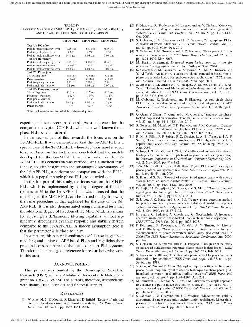
TABLE IVSTABILITY MARGINS OF MFOF-PLL1 , MFOF-PLL2 , AND MFOF-PLL3

AND DETAILS OF THEIR NUMERICAL COMPARISON

MFOF-PLL1 MFOF-PLL2 MFOF-PLL3

Test A∗: DC offsetPeak-to-peak frequency error 0.98 Hz 0.71 Hz 0.58 HzPeak-to-peak phase error 6.56◦ 4.79◦ 3.88◦

Peak-to-peak amplitude error 0.11 p.u. 0.08 p.u. 0.06 p.u.Test B∗: HarmonicsPeak-to-peak frequency error 0.15 Hz 0.18 Hz 0.22 HzPeak-to-peak phase error 0.98◦ 1.2◦ 1.48◦

Peak-to-peak amplitude error 0.03 p.u. 0.04 p.u. 0.04 p.u.Test C∗: Phase jump2% settling time 55.6 ms 54.6 ms 54.7 msPhase overshoot 21.57% 24.31% 24.35%Peak frequency variation 2.53 Hz 2.39 Hz 2.29 HzPeak amplitude variation 0.1 p.u. 0.08 p.u. 0.07 p.u.Test D∗: Frequency jump2% settling time 41.1 ms 40.7 ms 40.6 msFrequency overshoot 1.62% 1.64% 1.71%Peak phase variation 4.11◦ 4.16◦ 4.13◦

Peak amplitude variation 0.01 p.u. 0.01 p.u. 0 p.u.Phase margin 57◦ 55.7◦ 58.6◦


experimental tests were conducted. As a reference for thecomparison, a typical CCF-PLL, which is a well-known three-phase PLL, was considered.

In the second part of this research, the focus was on the1φ-APF-PLL. It was demonstrated that the 1φ-APF-PLL is aspecial case of the 3φ-APF-PLL where its β-axis input is equalto zero. Based on this fact, it was concluded that the modelsdeveloped for the 3φ-APF-PLL are also valid for the 1φ-APF-PLL. This conclusion was verified using numerical tests.Finally, to gain insight into the advantages/disadvantages ofthe 1φ-APF-PLL, a performance comparison with the EPLL,which is a popular single-phase PLL, was carried out.

In the last part of this study, the focus was on the MFOF-PLL, which is implemented by adding a degree of freedom(parameter k) to the 1φ-APF-PLL. It was discussed that themodeling of the MFOF-PLL can be carried out by followingthe same procedure as that explained for the case of the 3φ-APF-PLL. It was also demonstrated using numerical tests thatthe additional degree of freedom of the MFOF-PLL is a meansfor adjusting its dc/harmonic filtering capability without sig-nificantly affecting its dynamic response and stability margincompared to the 1φ-APF-PLL. A hidden assumption here isthat the parameter k is close to unity.

In summary, this paper disseminates useful knowledge aboutmodeling and tuning of APF-based PLLs and highlights theirpros and cons compared to the state-of-the-art PLL systems.Therefore, it can be a good reference for researchers who workin this area.

ACKNOWLEDGMENT

This project was funded by the Deanship of ScientificResearch (DSR) at King Abdulaziz University, Jeddah, undergrant no. (RG-9-135-38). The authors, therefore, acknowledgewith thanks DSR technical and financial support.

REFERENCES

[1] W. Xiao, M. S. El Moursi, O. Khan, and D. Infield, “Review of grid-tiedconverter topologies used in photovoltaic systems,” IET Renew. PowerGener., vol. 10, no. 10, pp. 1543–1551, 2016.

[2] F. Blaabjerg, R. Teodorescu, M. Liserre, and A. V. Timbus, “Overviewof control and grid synchronization for distributed power generationsystems,” IEEE Trans. Ind. Electron., vol. 53, no. 5, pp. 1398–1409,Oct. 2006.

[3] S. Golestan, J. M. Guerrero, and J. C. Vasquez, “Single-phase PLLs:A review of recent advances,” IEEE Trans. Power Electron., vol. 32,no. 12, pp. 9013–9030, Dec. 2017.

[4] S. Golestan, J. M. Guerrero, and J. C. Vasquez, “Three-phase PLLs: Areview of recent advances,” IEEE Trans. Power Electron., vol. 32, no. 3,pp. 1894–1907, Mar. 2017.

[5] M. Karimi-Ghartemani, Enhanced phase-locked loop structures forpower and energy applications. John Wiley & Sons, 2014.

[6] S. Golestan, J. M. Guerrero, A. Abusorrah, M. M. Al-Hindawi, andY. Al-Turki, “An adaptive quadrature signal generation-based single-phase phase-locked loop for grid-connected applications,” IEEE Trans.Ind. Electron., vol. 64, no. 4, pp. 2848–2854, Apr. 2017.

[7] S. Golestan, J. M. Guerrero, J. C. Vasquez, A. M. Abusorrah, and Y. Al-Turki, “Research on variable-length transfer delay and delayed-signal-cancellation-based PLLs,” IEEE Trans. Power Electron., vol. 33, no. 10,pp. 8388–8398, Oct. 2018.

[8] M. Ciobotaru, R. Teodorescu, and F. Blaabjerg, “A new single-phasePLL structure based on second order generalized integrator,” in 200637th IEEE Power Electronics Specialists Conference, Jun. 2006, pp. 1–6.

[9] Q. Guan, Y. Zhang, Y. Kang, and J. M. Guerrero, “Single-phase phase-locked loop based on derivative elements,” IEEE Trans. Power Electron.,vol. 32, no. 6, pp. 4411–4420, Jun. 2017.

[10] S. Golestan, M. Monfared, F. D. Freijedo, and J. M. Guerrero, “Dynam-ics assessment of advanced single-phase PLL structures,” IEEE Trans.Ind. Electron., vol. 60, no. 6, pp. 2167–2177, Jun. 2013.

[11] R. M. S. Filho, P. F. Seixas, P. C. Cortizo, L. A. B. Torres, and A. F.Souza, “Comparison of three single-phase PLL algorithms for UPSapplications,” IEEE Trans. Ind. Electron., vol. 55, no. 8, pp. 2923–2932,Aug. 2008.

[12] Y. Jung, J. So, G. Yu, and J. Choi, “Modelling and analysis of active is-landing detection methods for photovoltaic power conditioning systems,”in Canadian Conference on Electrical and Computer Engineering 2004,vol. 2, May. 2004, pp. 979–982.

[13] J.-W. Choi, Y.-K. Kim, and H.-G. Kim, “Digital PLL control for single-phase photovoltaic system,” IEE Proc.-Electric Power Appl., vol. 153,no. 1, pp. 40–46, Jan. 2006.

[14] S. Kim and S. Sul, “Control of rubber tyred gantry crane with energystorage based on supercapacitor bank,” IEEE Trans. Power Electron.,vol. 21, no. 5, pp. 1420–1427, Sep. 2006.

[15] D. Stojic, N. Georgijevic, M. Rivera, and S. Milic, “Novel orthogonalsignal generator for single phase PLL applications,” IET Power Elec-tronics, vol. 11, no. 3, pp. 427–433, 2018.

[16] S.-J. Lee, J.-K. Kang, and S.-K. Sul, “A new phase detecting methodfor power conversion systems considering distorted conditions in powersystem,” in Proc. Industry Applications Conf., 34th IAS Annu. Meeting,vol. 4, Oct. 1999, pp. 2167–2172.

[17] H. Sagha, G. Ledwich, A. Ghosh, and G. Nourbakhsh, “A frequencyadaptive single-phase phase-locked loop with harmonic rejection,” inIEEE IECON 2014, Oct. 2014, pp. 1028–1033.

[18] P. Rodriguez, R. Teodorescu, I. Candela, A. V. Timbus, M. Liserre,and F. Blaabjerg, “New positive-sequence voltage detector for gridsynchronization of power converters under faulty grid conditions,” in2006 37th IEEE Power Electronics Specialists Conference, Jun. 2006,pp. 1–7.

[19] S. Golestan, M. Monfared, and F. D. Freijedo, “Design-oriented studyof advanced synchronous reference frame phase-locked loops,” IEEETrans. Power Electron., vol. 28, no. 2, pp. 765–778, Feb. 2013.

[20] V. Kaura and V. Blasko, “Operation of a phase locked loop system underdistorted utility conditions,” IEEE Trans. Ind. Appl., vol. 33, no. 1, pp.58–63, Jan. 1997.

[21] X. Guo, W. Wu, and Z. Chen, “Multiple-complex coefficient-filter-basedphase-locked loop and synchronization technique for three-phase grid-interfaced converters in distributed utility networks,” IEEE Trans. Ind.Electron., vol. 58, no. 4, pp. 1194–1204, Apr. 2011.

[22] M. Ramezani, S. Golestan, S. Li, and J. M. Guerrero, “A simple approachto enhance the performance of complex-coefficient filter-based PLL ingrid-connected applications,” IEEE Trans. Ind. Electron., vol. 65, no. 6,pp. 5081–5085, Jun. 2018.

[23] S. Golestan, J. M. Guerrero, and J. C. Vasquez, “Modeling and stabilityassessment of single-phase grid synchronization techniques: Linear time-periodic versus linear time-invariant frameworks,” IEEE Trans. PowerElectron., vol. 34, no. 1, pp. 20–27, Jan. 2019.



[24] M. Karimi-Ghartemani, “Linear and pseudolinear enhanced phased-locked loop (EPLL) structures,” IEEE Trans. Ind. Electron., vol. 61,no. 3, pp. 1464–1474, Mar. 2014.

All-Pass-Filter-Based PLL Systems: Linear Modeling ...

Documents

Transcript of All-Pass-Filter-Based PLL Systems: Linear Modeling ...