Aggregate Implications of Indivisible Labor, Incomplete

Markets, and Labor Market Frictions∗

Per Krusell† Toshihiko Mukoyama‡ Richard Rogerson§ Aysegul Sahin¶

November 2007

Abstract

This paper analyzes a model that features frictions, an operative labor supply mar-

gin, and incomplete markets. We first provide analytic solutions to a benchmark model

that includes indivisible labor and incomplete markets in the absence of trading frictions.

We show that the steady state levels of aggregate hours and aggregate capital stock are

identical to those obtained in the economy with employment lotteries, while individual

employment and asset dynamics can be different. Second, we introduce labor market fric-

tions to the benchmark model. We find that the effect of the frictions on the response of

aggregate hours to a permanent tax change is highly non-linear. We also find that there is

considerable scope for substitution between “voluntary” and “frictional” nonemployment

in some situations.

Keywords : Indivisible Labor, Incomplete Markets, Labor Market Frictions

JEL Classifications : E24, J22, J64

∗We thank Gadi Barlevy and Bob Hall for comments. The views expressed in this article are those of the

authors and do not necessarily reflect the position of the Federal Reserve Bank of New York or the Federal

Reserve System.†Princeton University, CEPR, and NBER‡University of Virginia and CIREQ§Arizona State University and NBER¶Federal Reserve Bank of New York

1

1 Introduction

Although labor market outcomes have always figured prominently in macroeconomic anal-

yses, the way in which macroeconomists model the labor market has changed dramatically

over the last forty years. In particular, two underlying premises that bear on how to model

the labor market have become commonplace during this period: the first is the premise that

labor supply matters for aggregate labor market outcomes, and the second is the premise

that trading frictions matter for aggregate labor market outcomes. Interestingly, both of

these views can be traced to contributions that appeared in the Phelps (1970) volume, and

each represented a radical departure from the canonical macroeconomic model of that time

period. From the household perspective, the canonical model prevailing at the time assumed

that desired hours of work were independent of any features of the economic environment,

including such factors as wages, taxes and transfer programs, and from the firm perspective

this model assumed that employment could be costlessly and immediately increased in line

with any increase in the demand for labor.

Although these two premises are not in any sense in conflict, almost all work on aggregate

labor market outcomes adopts one or the other but not both. This is reflected in the fact

that the two standard frameworks for addressing issues related to the aggregate labor market

are either the one-sector growth model (extended to include an endogenous labor supply de-

cision as in Kydland and Prescott (1982)), or a version of the Diamond-Mortensen-Pissarides

matching model. The former abstracts from any trading frictions in the labor market, while

the latter abstracts from any labor supply considerations. One interpretation of this state

of affairs is that each feature is important for its own particular subset of issues; in fact,

however, both frameworks are routinely used to address the same set of issues, ranging from

the nature of business cycle fluctuations to the effect of permanent policy changes. Moreover,

in some cases the two models deliver results that are sharply different.

In view of this situation, we believe that it is important to develop a better understanding

of the relative importance of these two features for specific issues of interest. The goal of

2

this paper is to take a first step in this agenda. Specifically, the contribution of the paper is

twofold. First, we develop a general equilibrium model that incorporates both labor market

frictions and a standard labor supply problem. Second, we use our model to address one

important issue in aggregate labor market analysis: the effect of tax and transfer programs

on steady state hours of work. Following the work of Prescott (2004), this issue has attracted

considerable attention and serves as a useful starting point for thinking about the relative

importance of labor supply considerations and frictions.

The model that we develop possesses three key features: indivisible labor, frictions and

incomplete markets. If one wants to capture trading frictions in the labor markets, then

indivisible labor is a natural assumption. While one can certainly formulate models of indi-

visible labor and trading frictions with complete markets, we believe that a market structure

that does not include either markets for employment lotteries or insurance markets for the

idiosyncratic income shocks that frictions generate is of particular interest.

Our analysis provides several interesting results. First, we provide analytic solutions to

a benchmark model that includes indivisible labor and incomplete markets in the absence of

trading frictions. We show that steady state equilibrium allocations are identical to those

that obtain in the economy when one permits trade of employment lotteries. Our result

extends the similar finding of Prescott et al. (2007) that considered continuous time, finite

horizons, and no discounting.1 We also provide a complete characterization of the individual

decision rules that obtain in this equilibrium. Two interesting properties emerge. One is that

wealth effects are non-linear in wealth. For either low or high wealth, increases in wealth

lead to equal increases in consumption, but for intermediate levels of wealth the effect on

consumption is zero. In contrast, for low and high levels of wealth the effect of wealth on

labor supply is zero, but for intermediate levels the effect is positive, but only in a lifetime

sense. This follows from the other interesting property: current labor supply is indeterminate

for intermediate levels of wealth. Specifically, equilibrium imposes structure on the amount

1Also see Ljungqvist and Sargent (2007) and Nosal and Rupert (2007) for related analysis.

3

of labor supplied over one’s lifetime but imposes very little structure on the timing of labor

supply. This indeterminacy has important implications for how individuals respond to the

presence of frictions.

Second, we find that the extent to which labor market frictions affect the response of

aggregate steady state hours to permanent changes in tax and transfer programs is also

highly non-linear. Specifically, in some regions of the parameter space the presence of frictions

has effectively no effect on the response, while in other regions of the parameter space the

presence of frictions leads to a dramatic reduction in the response of hours of work. But

importantly, this effect is not linear. For example, in the case of tax reductions, the effect of

frictions may only manifest itself for reductions beyond some threshold. But the magnitude

of this threshold depends very much on the initial equilibrium: starting from some equilibria,

friction manifest themselves even for small changes. An important message is that one cannot

generally conclude that frictions do or do not matter for a specific issue. Whether they matter

depends very much on what region of the parameter space one is in and on the nature of the

policy change being considered.

Third, we find that there is considerable scope for substitution between “voluntary”

and “frictional” nonemployment in some regions. Specifically, an increase in frictions need

not have any effect on steady state equilibrium employment. Moreover, this remains true

even though the length of nonemployment spells is completely determined by the extent of

frictions.

An outline of the paper follows. In the next section we provide some background in-

formation that helps to describe the context of the more general research issue concerning

the interaction of labor supply and frictions. This section also summarizes some related

literature. Section 3 describes and analyzes the benchmark frictionless model that features

indivisible labor and incomplete markets. Section 4 introduces frictions into the model, and

Section 5 presents quantitative results for the effect of permanent tax changes and how the

effects depend upon frictions. Section 6 concludes and discusses directions for future research.

4

2 Background: Models with Indivisible Labor

We begin by describing two benchmark models that feature indivisible labor, one without

frictions and one with frictions. One is due to Hansen (1985) and the other is due to Pissarides

(1985).

2.1 Model Without Frictions

There is a continuum of mass one identical households, each with preferences over streams

of consumption and leisure given by:

E

[

∞∑

t=0

βt[α log ct + (1 − α) log(1 − ht)]

]

Labor is indivisible, which means that individuals can supply either 0 or h units of time to

market work in any period. There is an aggregate production function that uses capital and

labor as inputs:

yt = kθt h

1−θt

Output can be used as either consumption or investment, and capital depreciates at rate δ.

The calibration in Hansen (1985) leads to a steady state equilibrium with the following

features. (There are some important qualifications here that we will return to later.) Each

period a fraction e of the consumers are employed. Each period, these workers are chosen

randomly from the set of all workers. Everyone has constant and equal consumption over

time, independently of whether they work or do not work. So, the model generates an interior

value for the employment rate, and workers transition stochastically between employment

and non-employment.

2.2 Model With Frictions

Although there has been a virtual explosion in models featuring search frictions in the labor

market, for present purposes we want to focus on the simple Pissarides model, which we

think represents the simple or textbook version of a large class of these models. This model

5

features a continuum of mass one of identical workers. Labor is indivisible and each worker

has preferences defined by:

E

[

∞∑

t=0

βt[ct − bht]

]

where ht takes on the values zero or one. Output is produced by a matched firm-worker

pair. A match will produce output y. Existing matches end with exogenous probability λ

each period. These draws are iid across matches and across time. There is a technology for

creating matches. In particular, if there are ut unemployed workers at time t and vt vacancies

are posted at time t, then m(ut, vt) new matches will be created as of the beginning of period

t + 1. The function m is increasing in both arguments, is less than the min of its two

arguments and displays constant returns to scale. While search is assumed to be costless for

unemployed workers, it is assumed that the flow cost of posting a vacancy is k, measured

in units of output. There is no on the job search. The above information is sufficient

to formulate a social planner’s problem for this model. But if one wants to consider a

decentralized equilibrium then one needs some additional assumptions regarding how wages

will be determined. The standard assumption is that wages are determined via generalized

Nash bargaining in which the worker gets a share θ of the match surplus.

For a typical calibration, for example the one used by Shimer (2005), the steady state

equilibrium of this model has the following features. The employment (and nonemployment

or unemployment) rate is constant and lies strictly between zero and one. Workers transition

stochastically between the two states. The transition rate from employment to unemployment

is given by λ. Individual consumption fluctuates depending upon their employment status.

2.3 Comparison of the Two Models

At a superficial level, the nature of steady state allocations in these two models seem very

similar. Both models feature indivisible labor and generate steady states in which the em-

ployment rate is interior and workers move stochastically between employment and nonem-

6

ployment. Although these features are similar, the models might be viewed as connecting to

the data in slightly different ways—the indivisible labor model is probably best viewed as dis-

tinguishing between employment and nonemployment, without any implications for different

categories of nonemployment, i.e., unemployed versus nonparticipating. The matching model,

on the other hand, also has employed and nonemployed individuals, but the nonemployed in-

dividuals in this model seem to reflect what the data captures as unemployed workers rather

than non-participating workers. The matching model also has predictions for one variable

that the indivisible labor model does not—the number of vacancies that are posted.

Despite the superficial similarities between the two models, what we want to point out

next is that the two models are fundamentally different in terms of economic mechanisms.

Specifically, the indivisible labor model described above is fundamentally a model of labor

supply, and the changes in outcomes that result in this model when one adds shocks or

levies taxes reflect the response of labor supply to these changes. In contrast, the matching

model described abstracts completely from labor supply and is fundamentally a model of

endogenous frictions. When one adds shocks or levies taxes in this model and examines how

outcomes are altered, the mechanism reflects how these changes affect outcomes via changes

in the level of frictions.

2.3.1 Contrasting the Models: An Illustrative Example

To make this point it is useful to consider one specific example. In particular, we contrast the

results of Hansen (1985) and Shimer (2005) for the ability of technology shocks to account

for observed fluctuations in employment. (The Shimer paper was interested in a broader

set of outcomes than this, but for now we focus solely on the results for employment.)

Hansen concludes that technology shocks can account for much of the observed fluctuations

in employment, while Shimer concludes that they can account for virtually none. These

conclusions are dramatically different, and a naive reader of the literature might be tempted

to conclude that since the Shimer model looks like an indivisible labor model with frictions,

that adding frictions to the indivisible labor model greatly changes its properties. However, a

7

closer look at the two exercises reveals that such a conclusion is of course totally unwarranted.

Before we take this closer look, it is important to discuss one additional detail. In addition

to having frictions, the matching model also assumes noncompetitive wage setting, so one

needs to be careful about ascribing the differences in outcomes to the presence of frictions as

opposed to differences in wage setting. (Hall (2005) speaks to this issue. In his model, it is

differences in wage setting that are the key factor, and the presence of frictions serve simply

to rationalize the various wage setting rules.) However, since Shimer sets the bargaining

share parameter so that his equilibrium allocation is efficient, one can interpret the Hansen

and Shimer exercises as comparing efficient allocations in the presence of shocks, so that the

wage setting differences are not central.

Central to interpreting the differences in findings is the nature of the calibrated steady

states. In the Hansen calibration exercise, the parameter α dictates what fraction of the

population will be employed in the steady state. If this parameter is set sufficiently low,

implying that individuals do not value leisure very much, then the steady state equilibrium

will entail everyone employed. Given that in the data the employment to population ratio

is in the range of 0.60 − 0.65 depending upon what one views as the relevant population

base, Hansen chose α so that the steady state equilibrium matches this observation. That

is, in his steady state equilibrium, workers only want to spend roughly 60% of their lifetime

in employment. Next we consider this same issue in the context of the Shimer calibration.

An important property of the matching model described above is that it is linear. If one

removes the frictions from this model, then the steady state employment rate is dictated by

the relationship between the leisure parameter b and the productivity parameter y. More

specifically, if b < y then absent frictions, everyone will work every period. Conversely, if

b > y then no one will ever work (with or without frictions). In the knife-edge case of b = y

then everyone is always indifferent between working and nonworking so the equilibrium is

indeterminate in the absence of frictions. In order for his analysis to be of any interest,

Shimer necessarily calibrated his model so that b < y, in fact, he chose b = 0.4 and y = 1,

8

so that the difference is quite large. Given this choice, the frictionless version of his model

implies that everyone works all the time. In other words, he calibrates the model so that

the labor supply decision is degenerate. If one is going to compare his results to those of

Hansen, it is important to ask what would Hansen have found if he calibrated his model

to as to make the labor supply decision degenerate. This would amount to choosing the

value of α so that steady state employment is at a corner solution, equal to 1, and that the

solution is a long way from being interior. If Hansen had made this choice, he would have

found a dramatically different answer to the question of interest. In particular, he would have

concluded that technology shocks can account for none of the fluctuations in employment.

Shimer does not find that technology shocks account for none of the fluctuations in em-

ployment, rather he finds that technology shocks account for only a very small fraction of

fluctuations in employment. In Shimer’s model the only mechanism through which employ-

ment can fluctuate is through fluctuations in the level of frictions (i.e., the v/u ratio). What

we should conclude from his analysis is simply that fluctuations in the level of frictions is

not very important as a source of fluctuations in employment. What we learn from Hansen’s

exercise is that fluctuations in labor supply are an important source of fluctuations in employ-

ment. So while on the surface it seems that both papers are about the ability of technology

shocks to account for fluctuations in employment, the two papers are really about the ability

of two different propagation mechanisms by which technology shocks can induce fluctuations

in employment.

2.4 Discussion

In the context of the specific example just discussed, our analysis suggests what we find to

be an open and interesting question: What are the properties of models which feature both

non-trivial labor supply decisions and search frictions? This basically calls for a merging of

the two frameworks discussed earlier, which one can view as either adding labor supply to

the matching model or adding frictions to the indivisible labor model. Two remarks are in

order here. First, there are many search models that feature some aspect of labor supply.

9

In this regard this issue is not simply to add labor supply but to add it in a manner that

would allow the model to be consistent with applied work on labor supply. In particular,

specifications that feature linear utility are ultimately going to be of little interest. Second,

one should not think that adding labor supply to the matching models is synonymous with

adding curvature. As our discussion of the Hansen model indicates, the mere presence of

curvature in preferences does not imply that an indivisible labor model will feature a non-

generate labor supply decision.

In fact, some work has been done on models that feature non-degenerate labor supply

models and search frictions. Two early ones were Merz (1995) and Andolfatto (1996). These

papers essentially introduce the features of vacancy posting costs and a matching function

into an otherwise standard version of the growth model with indivisible labor. These authors

analyze allocations that solve a social planner’s problem and as such their analysis should

be interpreted as representing complete markets equilibrium allocations. The basic finding is

that the main business cycle predictions of the standard model were affected relatively little

by the introduction of search frictions. (We note parenthetically that this result might be

interpreted as a precursor to Shimer’s finding. If it were the case that search frictions matter

a lot for the propagation of shocks, then one might have expected that Andolfatto and Merz

would have found much larger fluctuations in labor as a result of adding frictions.) One dif-

ference noted by Andolfatto had to do with the dynamics of output and productivity—search

frictions basically induce a delay in the response of employment and can therefore generate

hump shaped impulse response curves for output. We interpret these findings to suggest that

if one is looking for settings in which frictions per se (and not wage determination) matter

in these models, that one should probably move away from the complete markets model.

It is of interest to talk briefly about incomplete markets models. One class of incom-

plete markets models that aggregate economists have found to be very useful are those in

the tradition of Aiyagari, Bewley, and Huggett. These are models in which individuals face

idiosyncratic income shocks but do not have access to insurance markets. There is a market

10

for one-period ahead borrowing and lending, but individuals face a limit on how much they

can borrow. Economists have found this to be a useful framework for a variety of issues.

It is of interest to note that the original models in this class also did not incorporate a

labor/leisure decision. However, subsequent work has incorporated this margin and many

additional insights have emerged. For example, Chang and Kim (2006) show that micro and

macro labor supply elasticities need not be the same, and in particular, macro elasticities

may be much larger than micro elasticities. Domeij and Floden (2006) show that standard

micro labor supply elasticities may be downward biased by a significant amount in such an

environment. Chang and Kim (2007) show that aggregate fluctuations in such an environ-

ment produce large fluctuations in the “Hall residual” that match those found in the data.

And Pijoan-Mas (2006) finds that this setting has important implications for how individuals

use precautionary savings as opposed to labor supply to self insure. In particular, he finds

that labor supply is inefficiently large in terms of total hours, and inefficiently low in terms

of effective units of labor input. Krusell and Smith (1998) show that business cycle fluctu-

ations induced by aggregate productivity shocks look very similar to those in the complete

markets economy, although there are some notable differences, specifically in the properties

of consumption relative to income. It is also important to note another issue raised by

the Krusell-Smith paper, which is computational. In particular, in moving from complete

markets models to incomplete markets models, in some contexts, such as the business cycle

context, there were serious computational issues that needed to be addressed before one could

assess whether incomplete markets matter. Krusell and Smith came up with one method that

works well for a certain class of incomplete markets models.

2.5 Summary

The preceding discussion has been a somewhat roundabout discussion of the literature to

suggest that the analysis of standard growth model-type environments that feature indivis-

ible labor, search frictions and incomplete markets is on the one hand relatively uncharted

territory, but at the same time territory that is very important for us to chart in order to

11

better understand what role frictions play in the context of various aggregate issues. There

are many possible findings that may emerge. We may find that some aggregates behave very

differently in the presence or absence of frictions and incomplete markets, or that aggregates

behave very similarly in the two contexts. Of particular interest here is the extent to which

adding frictions to the indivisible labor model might mute the size of employment fluctuations

in response to productivity shocks. It may be that aggregates are similar but that individual

level observations are very different, so that incorporating frictions and incomplete markets

provides a consistent framework in which we understand a larger set of observations. For

example, the indivisible labor model might not do a good job of accounting for the patterns

we see in individual employment histories, and adding frictions may help in this dimension.

As noted above, each model makes predictions about particular variables in the data that the

other does not—the indivisible labor model makes predictions about the size of the nonem-

ployed population, while the matching model seems only to make predictions about the size

of the unemployed population. And the matching model makes predictions about vacancies

that the indivisible labor model does not. It is unclear to what extent the more general

model can account for all observations simultaneously and what issues might arise. Or it

may be that frictions and incomplete markets do not change predictions but that a model

with these two features provides a richer setting in which we can analyze a wider set of issues.

It may also be that be the case that solving these models may require the development of

new methods. The objective of this paper is to explore these issues. Aside from the general

objective of exploring these issues, there is no specific result that we seek to confirm.

The framework might also have very interesting implications in the context of hetero-

geneous agents. We offer one example here. Shimer argues that layoff rates cannot drive

cyclical employment rate fluctuations because they produce an inconsistency with the Bev-

eridge curve. But if one considers a more general model it may be that layoffs are the

dominant source of fluctuations for some groups while labor supply considerations are the

dominant source of fluctuations for other groups, and that by combining these the aggregate

12

Beveridge curve is well behaved. Loosely speaking, one might imagine that for many prime

aged workers it is the increase in layoff rates coupled with search frictions that accounts

for much of their cyclical fluctuations in employment, while for younger workers and less

attached workers layoffs play very little role.

3 A Frictionless Benchmark Economy

As stated in the previous section, our objective is to study a class of models that features

indivisible labor, incomplete markets and frictions. The perspective that we adopt in this

work is to ask how the addition of frictions to an indivisible labor model with incomplete

markets affects the implications of the model. In view of this it is natural to consider a

benchmark model that features no frictions, indivisible labor and incomplete markets. We

begin by exploring this benchmark for a simple model with homogeneous individuals and no

aggregate shocks.

3.1 Environment

The environment is basically the same as that in Hansen (1985), except that we rule out all

insurance markets and trade in employment lotteries. Instead, following Krusell and Smith

(1998), we consider a market structure in which individuals can only hold capital as an asset.

The specifics of the model follow.

There is a continuum of measure one of identical households, each with preferences given

by:

E

[

∞∑

t=0

βt[log(ct) − d(ht)]

]

where ct ≥ 0 is consumption in period t and ht ∈ {0, 1} is hours devoted to market work

in period t. Given that labor is assumed to be indivisible we need only assume that d is

increasing. The discount factor β satisfies 0 < β < 1.

There is an aggregate production function that uses capital (Kt) and labor (Ht) to produce

13

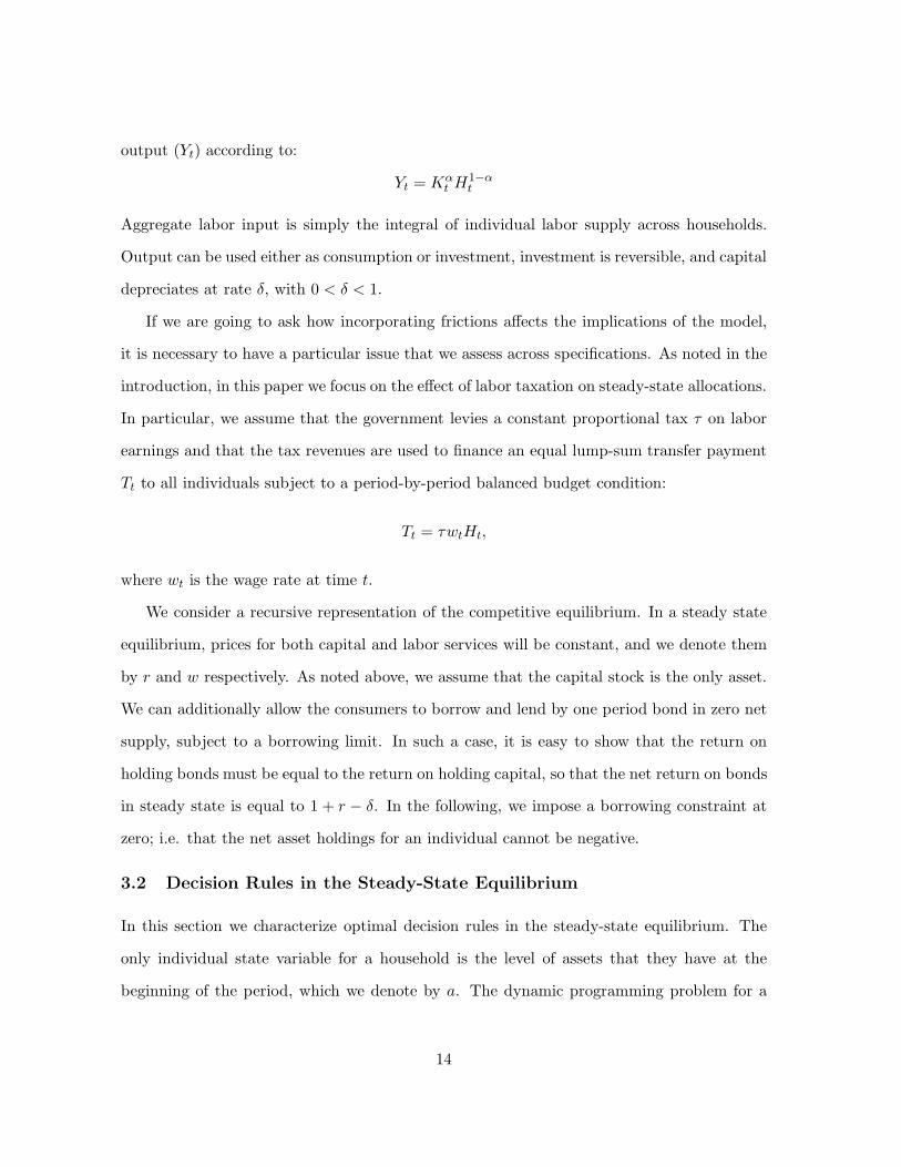
output (Yt) according to:

Yt = Kαt H1−α

t

Aggregate labor input is simply the integral of individual labor supply across households.

Output can be used either as consumption or investment, investment is reversible, and capital

depreciates at rate δ, with 0 < δ < 1.

If we are going to ask how incorporating frictions affects the implications of the model,

it is necessary to have a particular issue that we assess across specifications. As noted in the

introduction, in this paper we focus on the effect of labor taxation on steady-state allocations.

In particular, we assume that the government levies a constant proportional tax τ on labor

earnings and that the tax revenues are used to finance an equal lump-sum transfer payment

Tt to all individuals subject to a period-by-period balanced budget condition:

Tt = τwtHt,

where wt is the wage rate at time t.

We consider a recursive representation of the competitive equilibrium. In a steady state

equilibrium, prices for both capital and labor services will be constant, and we denote them

by r and w respectively. As noted above, we assume that the capital stock is the only asset.

We can additionally allow the consumers to borrow and lend by one period bond in zero net

supply, subject to a borrowing limit. In such a case, it is easy to show that the return on

holding bonds must be equal to the return on holding capital, so that the net return on bonds

in steady state is equal to 1 + r − δ. In the following, we impose a borrowing constraint at

zero; i.e. that the net asset holdings for an individual cannot be negative.

3.2 Decision Rules in the Steady-State Equilibrium

In this section we characterize optimal decision rules in the steady-state equilibrium. The

only individual state variable for a household is the level of assets that they have at the

beginning of the period, which we denote by a. The dynamic programming problem for a

14

household is then given by:

V (a) = max { maxa′

log(

(1 + r − δ)a + (1 − τ)w + T − a′)

− d(1) + βV (a′),

maxa′

log(

(1 + r − δ)a + T − a′)

− d(0) + βV (a′) }

subject to

a′ ≥ 0.

The Euler equation for this problem is

1

c= β(1 + r − δ)

1

c′,

regardless of the labor/leisure decision, where c′ is next period’s consumption. Thus, for

aggregate consumption to be constant, it is necessary that 1 + r − δ = 1/β. In what follows

we will replace 1 + r − δ by 1/β.

We further assume that β > 1/2. Let D ≡ d(1) − d(0) > 0. The following proposition

characterizes both the decision rules and the value function for the above problem.

Proposition 1 In the steady-state equilibrium, a worker’s decision rules on asset accumu-

lation and the work-leisure choice are summarized by the following five cases, based on the

level of the current asset a. Let I be indicator function which takes 1 when working and 0

when not working.

• Case 1: When a ≤ a:

a′ = a,

c =1 − β

βa + (1 − τ)w + T,

and

I = 1.

• Case 2: When a ∈ (a, a∗):

a′ =1

βa + (1 − τ)w + T −

(1 − τ)w

D,

15

c =(1 − τ)w

D,

and

I = 1.

• Case 3: When a ∈ [a∗, a∗]:

Indifferent between

a′ =1

βa + (1 − τ)w + T −

(1 − τ)w

D,

c =(1 − τ)w

D,

and

I = 1;

and

a′ =1

βa + T −

(1 − τ)w

D,

c =(1 − τ)w

D,

and

I = 0.

• Case 4: When a ∈ (a∗, a):

a′ =1

βa + T −

(1 − τ)w

D,

c =(1 − τ)w

D,

and

I = 0.

• Case 5: When a ≥ a:

a′ = a,

c =1 − β

βa + T,

16

Figure 1: Decision rules for work-leisure choice

and

I = 0.

Here, the thresholds on a are defined as the following.

a =β((1 − τ)w − D((1 − τ)w + T ))

(1 − β)D,

a =β((1 − τ)w − DT )

(1 − β)D,

a∗ = a + β(1 − τ)w,

and

a∗ = a − β(1 − τ)w.

Note that a − a = β(1 − τ)w/(1 − β). Also note that a > a∗ > a∗ > a holds.

Figures 1, 2, and 3 depict the decision rules for the work-leisure choice, the asset choice,

and consumption. Intuitively, we can interpret the result as three different types of behavior,

depending on the level of wealth, with two “buffer zones” in between.

17

Figure 2: Decision rules for asset choice

Figure 3: Decision rules for consumption

18

When the wealth level is very low (a ≤ a: “work” region), the consumer always works,

and the asset level remains constant over time. In this region, a higher wealth level means a

higher level of consumption. In contrast, when the wealth level is very high (a ≥ a: “leisure”

region), the consumer never works, but the asset level again remains constant over time. As

in the previous case, a higher wealth level means a higher consumption. A worker who starts

in either of these two regions of wealth will have the same values for h, a, and c forever.

Next we consider the case in which the wealth level is intermediate (a ∈ [a∗, a∗]: “indif-

ference” region). In this region the consumer is indifferent between working and not working

in the current period. In general, the consumer will move between periods of work and

periods of leisure, but consumption remains constant independently of the current work de-

cision. During a period of work, the consumer accumulates assets, and during a period of

leisure, the consumer runs down their assets. In this region, the consumption level is con-

stant across different wealth levels, but the wealth level changes over time. Many different

dynamic work/leisure patterns for the consumer are possible, though this will be clearer once

we discuss the role of the “buffer zones.”

Between the “work” region and the “indifference” region and between the “indifference”

region and the “leisure” region, there are “buffer zones.” Starting from these zones, the asset

level always moves towards the “indifference” region. Workers who start with wealth levels

in the “indifference” region can enter these buffer zones, but they are always brought back to

the “indifference” region. They will never leave the interval consisting of the “indifference”

region and the two buffer zones. In the buffer zones, the consumption level is the same as in

the “indifference” region. Although the labor decision is not determined inside the region of

indifference, if a given household were to repeatedly choose to not work (or work), then they

would eventually transit to the buffer zone that lies below (above) the indifference region, and

at this point the labor supply decision becomes determinate until they once again enter the

indifference region. It follows that the equilibrium places some discipline on the number of

consecutive periods of employment or non-employment, but apart from this places relatively

19

few restrictions on the nature of individual employment histories.

It is of interest to consider the issue of how large the various regions are, and how

they respond to changes in various parameters. One can show that if β tends to one, the

relative size of the buffer zones (compared to the size of the indifference zone) tends to

zero. This finding is intuitive. In a continuous time model the buffer zones would not exist;

instead we would simply have reflecting barriers on either end of the indifference region. One

interpretation of the case where β tends to one is that we are making each period very very

short, and hence we approach the continuous time result.

An interesting implication of the above characterization is that a wealth transfer has

very different effects on consumption, depending on the initial level of wealth. When the

wealth level is very low or very high, a (small) transfer in wealth increases the worker’s

consumption level, but has no impact on hours of work. However, the consumption level is

unaffected by a (small) transfer if the wealth level is in the “indifference” region. There, an

increase in wealth is perfectly absorbed by an increase in leisure time, though not necessarily

contemporaneously. In other words, there is no wealth effect in consumption decision in this

region. Similarly, the effects of a wealth transfer on labor supply is also very dependent on

the initial wealth holdings and can be very non-linear in the amount of the transfer. For

example, a positive wealth transfer can push a household from the region of always working

to the indifference region, but for smaller wealth transfer there might not be any effect.

Although we will not pursue the issue further here, we think it is interesting to note that

the above characterization has some interesting implications for empirical work that seeks

to uncover various labor supply elasticities. Specifically, the fact that current labor supply

does not respond to an increase or decrease in wealth is potentially not at all informative

regarding the overall effect on labor supply. The associated changes in labor supply may

occur in the future instead of contemporaneously.

Although individuals who lie in the indifference region do not have a uniquely determined

labor supply in steady state equilibrium, steady state equilibrium does not allow all individu-

20

als to arbitrarily choose their labor supply. The reason for this is that the steady state values

of r and w are only consistent with a given aggregate level of labor supply. We consider the

aggregate implications in the next subsection.

3.3 Steady State Equilibrium

In this subsection we show that the aggregate steady state equilibrium allocations in the

incomplete market economy described above are in fact identical to those that would obtain

if one allowed trade in employment lotteries. This result is similar to the one obtained by

Prescott et al. (2007) but in a different setting. They assumed continuous time, finite lifetimes

and no discounting, whereas our analysis has discrete time, infinite lives and discounting. We

begin by characterizing the aggregate steady state equilibrium allocation for the incomplete

market economy.

In equilibrium, K is equal to the sum of the individual asset holdings a and H is equal

to the mass of individuals who decide to work. From the first-order conditions of the firm,

r = α

(

K

H

)α−1

and

w = (1 − α)

(

K

H

)α

hold. From the worker’s Euler equation,

1

β= 1 + α

(

K

H

)α−1

− δ (1)

holds.

Integrating across all the workers’ budget constraints we have that:

K =1

βK + w(1 − τ)H + T − C. (2)

Given that the government balances its budget each period, we have τwH = T .

Further, assume that this economy has workers only in (a, a) region. Then, everyone has

consumption given by (1 − τ)w/D. Then,

K =1

βK + (1 − α)

(

K

H

)α

H −(1 − τ)(1 − α)

(

KH

)α

D(3)

21

holds. We can obtain K and H by solving (1) and (3). T can then be calculated as T = τwH.

The next proposition compares the allocation of this model to the complete-market lottery

model of Rogerson (1988).

Proposition 2 Consider a complete-market version of our model, where an employment

lottery is available. The aggregate allocation, K and H, are identical between this complete-

market model and the incomplete-market model.

Proof: When an employment lottery is available in a complete-market setting, in the

steady state a worker solves the following problem:

V (a) = maxa′,λ

log(

(1 + r − δ)a + λ(1 − τ)w + T − a′)

− λd(1) − (1 − λ)d(0) + βV (a′),

where λ is the employment probability. The first-order condition for the asset choice yields

1

c= β(1 + r − δ)

1

c′,

so again, in steady-state, 1/β = (1 + r − δ) has to hold. Since the firm’s first-order condition

is identical to the incomplete-market case, equation (1) has to hold in this model.

Note that λ = H in equilibrium. Summing up the budget constraint in this economy

yields the same equation as (2). The first-order condition for λ yields

(1 − τ)w1

c= D,

therefore

c =(1 − τ)w

D.

Note that this is identical to the incomplete-market case. Thus, the equation (3) holds in the

complete-market economy. Since K and H solve (1) and (3) in both economies, the solution

has to be identical. �

It follows that the aggregate behavior of the incomplete-market economies is the same as

the complete-market economy, although the individual behavior of employment and asset

dynamics may look very different.

22

4 Frictions in the Benchmark Economy

We now introduce frictions to the labor market. Our approach to modeling frictions is in

the spirit of the island model of Lucas and Prescott (1974), though our environment differs

from theirs in some respects. In particular, we will assume that there are two islands, one

of which we call the “production island,” and the other of which we will call the “leisure

island.” The production island is endowed with an aggregate production function that is

the same as that considered in the benchmark model in the previous section. We introduce

frictions by assuming that workers cannot freely move between the two islands. In particular,

if a worker supplies labor in period t (i.e., resides on the production island in period t), then

with probability σ they will begin the next period on the leisure island, and with probability

1 − σ they will begin the next period on the production island. At the beginning of period

t + 1, any individual who either did not supply labor in period t (i.e., lived on the leisure

island in period t) or was sent to the leisure island at the end of period t, will be sent to

the production island with probability λw. These workers, plus any workers who resided

on the production island in period t and were not sent to the leisure island, all have the

opportunity to supply labor in period t + 1. All other workers do not have the opportunity

to supply labor in period t + 1. Loosely speaking, σ is the exogenous separation rate, and

λw is the exogenous job arrival rate. Note that given this formulation, the frictionless model

in the previous section corresponds to the case with λw = 1, since if all workers always have

a job offer, then separations are irrelevant. The key feature of this economy relative to the

benchmark model is that workers do not always have the opportunity to work. This manifests

itself in two different ways. First, if an individual chooses to not work in period t, then it is

not certain that he or she will have the opportunity to work in period t + 1. Second, even if

an individual works in period t, he or she is not guaranteed an opportunity to work in period

t + 1.

Once again we will focus on a steady state equilibrium. We assume the same market

structure as before, i.e., markets for output, labor and capital services in each period, in

23

addition to a one period bond. We again denote steady state values for the wage and rental

rate for capital services as w and r. A worker’s state consists of their location at the time

that the labor supply decision needs to be made, and the level of asset holdings. Let the value

function for a worker in a productive island be W (a), the value function for a worker who

begins the period on the leisure island but before the job offer realization be S(a), and the

value function for a worker who does not work for the current period (nonemployed worker)

be N(a). Then, the Bellman equation for an individual who has the opportunity to work

and chooses to work is:

W (a) = maxc,a′

log(c) − d(1) + βE[σS(a′) + (1 − σ)max{W (a′), N(a′)}]

subject to

a′ = (1 + r − δ)a + (1 − τ)w + T − c

and

a′ ≥ 0.

The worker who begins a period on the leisure island has the Bellman equation given by:

S(a) = λw max{W (a), N(a)} + (1 − λw)N(a).

And an individual who does not work, either because they did not have the opportunity or

chose not to, has a Bellman equation given by:

N(a) = maxc,a′

log(c) − d(0) + βS(a′)

subject to

a′ = (1 + r − δ)a + T − c

and

a′ ≥ 0.

The firm and the government is formulated the same way as in the previous section, so

we do not repeat them here.

24

The economy with frictions does not permit as sharp an analytical characterization as

was possible for the frictionless model. However, some properties can be established. For

example, the decision rule for whether to work has a reservation property with regard to

asset holdings. In particular, if it is not optimal for a worker with asset holdings a to work,

then any individual with assets greater than a will also find it not optimal to work. Similarly,

if an individual with asset holdings a finds it optimal to work, then any individual with asset

holdings less than a will choose to work given the opportunity.

Note that adding frictions to the model serves to break the indeterminacy result that

we found for the frictionless model. There we found a region of asset holdings for which

the individual was indifferent regarding current labor supply, but with frictions this region

shrinks to a single point. An important quantitative issue is that there may still be a region

in which the individual is very close to indifference, so that even when the individual strictly

prefers to work this period, it may not matter much to them.2

In contrast to the frictionless model, it will not be that the case that 1/β = 1+r−δ in the

steady state equilibrium. The presence of frictions implies that individuals face idiosyncratic

income risk, and as is standard in models with idiosyncratic income risk and incomplete

markets, we will have greater accumulation of capital.

5 Implications of Frictions: Quantitative Results

In this section we analyze how labor market frictions impact the answer to a simple tax

experiment. Specifically, we consider tax policies of the form described earlier, in which the

government levies a constant proportional tax on labor earnings and uses the proceeds to

fund a uniform lump-sum transfer to all individuals, subject to a period-by-period balanced

budget rule. We examine how the presence of frictions affects the response to a tax changes

of a given magnitude.

2Idiosyncratic variation in either productivity or preferences can also serve to break the indifference in the

frictionless model. Rogerson and Wallenius (2007) use age varying productivity or disutility from working

to generate determinate labor supply patterns over the lifecycle. Chang and Kim (2006) use idiosyncratic

productivity shocks to generate determinate labor supply patterns.

25

5.1 Calibration

In this subsection we describe how we calibrate the model. We will consider different levels

of frictions, but for our benchmark calibration we will also calibrate the parameters that

characterize the frictions. We set the period length equal to one month. Many of the

parameters can be calibrated using standard methods. Specifically, we choose values for

β, α, and δ so as to match three targets: a capital share of 0.3, an investment to output

ratio of 0.2, and a 4% annual rate of return to capital. This gives β = 0.9967, α = 0.3

and δ = 0.0067. We set τ = 0.30 as the tax rate, consistent with measured values of the

current average effective tax rate on labor income for the US. For the two parameters that

capture the extent of frictions we set λw = 0.2 and σ = 0.02. These values are consistent

with the transition probabilities between unemployment and employment in the CPS data.3

We normalize d(0) = 0 and set d(1) = −2.3 × log(1 − 1/3). From these, we obtain that 66%

of the population is working in the steady-state of the benchmark, which is similar to the

employment to population ratio in the United States.

As noted above, we will also consider economies with different levels of frictions in order

to assess the importance of frictions for the answer to a specific policy question. Specifically,

we will consider various values of λw, holding σ constant. In these economies with different

values of λw we recalibrate all of the other parameters of the model so as to match the same

aggregate targets, i.e., capital’s share of income, the investment to output ratio, the real rate

of return to capital and the employment rate.

One of the economies that we study is the frictionless benchmark economy. When con-

sidering the frictionless model we assume that all the workers start from the wealth level

in the “indifference” region. As noted earlier, there is a large indeterminacy in the decision

rules of the workers in the “indifference” region. However, in the presence of frictions this

3See Hobijn and Sahin (2007, Table 3). They report that the transition rate from unemployment to

employment is on average 20 percent for 1976-2005. Consistent with this, we set λw = 0.2 for our benchmark

calibration. Hobijn and Sahin also report that employment to unemployment transition rate is on average

1.6 percent for the same sample period. Since λw = 0.2 fraction of unemployed workers find jobs in the same

period, we set σ = 0.02 which is consistent with a transition rate of 1.6 percent.

26

K/H

λw = 1.0 128.7

λw = 0.3 128.7

λw = 0.2 129.0

λw = 0.1 131.8

Table 1: Capital-labor ratio

indeterminacy does not exist–instead there are reservation asset levels. If we want to think

of the frictionless economy as the limit of the economy with frictions as the level of frictions

tend to zero then it seems reasonable to focus on decision rules for the frictionless economy

which also impose a reservation asset rule, and so we do this when solving for the equilibrium

of the frictionless model. We let the threshold asset holdings be denoted by a: work when

a ≤ a and take leisure when a > a. Although there are many values of a that are consistent

with optimal decision rules, there is only once choice of a that is consistent with the steady

state aggregate values of K and H. It is typically the case that K is increasing in a, so a

can be pinned down by the aggregate values of K implied by (1) and (3).

We consider four values for λw: 1.0 (no frictions), 0.3, 0.2, and 0.1. Although the targets

used in the calibration are the same across all economies, the economies do differ along some

dimensions that are not targeted. Table 1 shows the values of capital-labor ratio K/H for

the various calibrated economies.

Given that aggregate employment is the same across all four economies, these differences

reflect differences in capital accumulation. Note that this value is the same for λw = 1.0

and λw = 0.3, but that it increases as λw is decreased further. Given the literature on

precautionary savings (see e.g., Huggett (1993)), it is intuitive that K/H increases as frictions

increase, since greater frictions lead to greater uncertainty in the individual income process,

and therefore additional precautionary savings. What the table tells us is that this effect only

becomes quantitatively noticeable when frictions are quite large, since even when λw = 0.3

the amount of capital accumulated is effectively identical to that in the frictionless economy.

27

Equilibrium Frictional Nonemployment Only

Employment Nonemployment Employment Nonemployment

λw = 1.0 1.9 1.0 − −

λw = 0.3 6.4 3.3 71.4 3.3

λw = 0.2 9.6 5.0 62.5 5.0

λw = 0.1 19.1 10.0 55.6 10.0

Table 2: Average duration of employment and nonemployment

Key to this result is the fact that in our calibrated economy, individuals only want to work

roughly two-thirds of the time. This makes it easy for the individuals to accommodate some

frictional nonemployment. For example, if an individual in the frictionless economy were

simply told that they would not be allowed to work every tenth period, this would have no

effect on their accumulation of assets.

It is also of interest to examine how individual employment histories vary with the extent

of frictions. Table 2 presents the average duration of employment and nonemployment spells

in steady state equilibrium for the four different economies.

The final two columns report the duration of employment and nonemployment spells that

would result if there were only frictional nonemployment. Interestingly, the average duration

of nonemployment spells in all of the economies with frictions is exactly that which would

emerge if all nonemployment were frictional. It follows that individuals in these economies

effectively never turn down an employment opportunity. To understand this result, note that

any individual who has spent one period not working must necessarily have asset holdings

below the reservation asset level. If they are nonemployed because of job loss, then their

assets at the time of job loss must have been below the reservation level, and spending

one period without working will have reduced them further. If, on the other hand they

became nonemployed by choice, by virtue of having spent a period in unemployment they

will necessarily have reduced their asset holdings.4 Because the steady state employment

4Of course, a worker who suffered a job loss at the end of period t but who would have chosen not to work

in period t + 1 will not accept a job opportunity in period t + 1 even if offered.

28

rate is above 0.5, it must be that one period of unemployment necessarily pushes their assets

below the reservation level. It follows that no-one who has spent one period unemployed ever

turns down a job opportunity. One might conjecture that if individuals never turn down job

offers, then employment must be determined by the frictions. However, this table shows that

employment spells are much shorter than that which would obtain in an economy in which

nonemployment were only due to frictions. In other words, labor supply considerations are

very much at work in equilibrium even though all unemployed workers will always accept an

offer to work.

The table also shows that a key impact of frictions is to change the nature of individ-

ual employment histories. In particular, as frictions increase, the average duration of both

employment and nonemployment spells increase. Average employment durations respond to

changes in λw even though the probability of job loss is constant across these economies. The

reason for this is that when λw is low, a worker knows that if they choose not to work today,

it may be several periods before they get another opportunity to work. Since they need to

have sufficient assets to provide for consumption during this nonemployment spell, they need

to work longer to accumulate more assets before choosing to not work in an economy with

low λw.

It is also of interest to examine the difference in asset distributions across the four

economies. This is done in Figures 4 and 5.

As one might expect from the previous intuition, as frictions increase the asset distribu-

tions become more spread out.

5.2 Results

In this subsection we report the effects of changes in taxes on steady state allocations for the

four economies that differ in the extent of frictions.

We begin by examining the effects on aggregate employment. Table 3 presents the results.

Recall that the calibration set τ = 0.30, so that by construction, employment is the same for

all four economies for this value of the tax rate.

29

0 50 100 1500

0.005

0.01

0.015

0.02

0.025

0.03

a

dens

ity

λw

=0.3

λw

=0.2

λw

=0.1

No friction

Figure 4: Wealth distributions for employed workers, τ = 0.30

0 50 100 1500

0.005

0.01

0.015

0.02

0.025

0.03

a

dens

ity

λw

=0.3

λw

=0.2

λw

=0.1

No friction

Figure 5: Wealth distributions for nonemployed workers, τ = 0.30

30

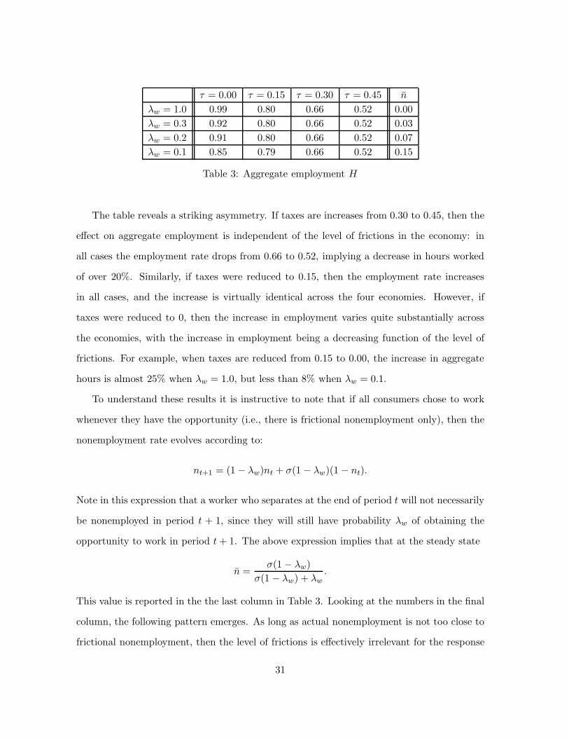
τ = 0.00 τ = 0.15 τ = 0.30 τ = 0.45 n

λw = 1.0 0.99 0.80 0.66 0.52 0.00

λw = 0.3 0.92 0.80 0.66 0.52 0.03

λw = 0.2 0.91 0.80 0.66 0.52 0.07

λw = 0.1 0.85 0.79 0.66 0.52 0.15

Table 3: Aggregate employment H

The table reveals a striking asymmetry. If taxes are increases from 0.30 to 0.45, then the

effect on aggregate employment is independent of the level of frictions in the economy: in

all cases the employment rate drops from 0.66 to 0.52, implying a decrease in hours worked

of over 20%. Similarly, if taxes were reduced to 0.15, then the employment rate increases

in all cases, and the increase is virtually identical across the four economies. However, if

taxes were reduced to 0, then the increase in employment varies quite substantially across

the economies, with the increase in employment being a decreasing function of the level of

frictions. For example, when taxes are reduced from 0.15 to 0.00, the increase in aggregate

hours is almost 25% when λw = 1.0, but less than 8% when λw = 0.1.

To understand these results it is instructive to note that if all consumers chose to work

whenever they have the opportunity (i.e., there is frictional nonemployment only), then the

nonemployment rate evolves according to:

nt+1 = (1 − λw)nt + σ(1 − λw)(1 − nt).

Note in this expression that a worker who separates at the end of period t will not necessarily

be nonemployed in period t + 1, since they will still have probability λw of obtaining the

opportunity to work in period t + 1. The above expression implies that at the steady state

n =σ(1 − λw)

σ(1 − λw) + λw

.

This value is reported in the the last column in Table 3. Looking at the numbers in the final

column, the following pattern emerges. As long as actual nonemployment is not too close to

frictional nonemployment, then the level of frictions is effectively irrelevant for the response

31

of aggregate employment to changes in taxes. But as the two values become closer, frictions

start to have an effect. Interestingly, however, it is not the case that frictions matter only

if the frictions bind in terms of the maximal steady state employment rate. For example,

consider a reduction of τ from 0.15 to 0.00 in the λw = 1.0 and λw = 0.3 economies. When

τ = 0.15, both economies have employment rates of 0.80. As taxes are decreased from 0.15

to 0.00, the frictionless economy has employment increase from 0.80 to 0.99. The maximal

steady state employment rate in the λw = 0.3 economy is 0.97. But the employment rate in

the λw = 0.3 increases only to 0.92 when taxes drop to 0.00, substantially below the maximal

level dictated by the frictions. Note that whether we are considering raising taxes from 0.00

to 0.15 or lowering taxes from 0.15 to 0.00, the elasticity of employment with regard to taxes

is less in the λw = 0.3 economy than in the λw = 1.0 economy.

To summarize, a key implication of these results is that in economies where individuals

do not desire to work in every period, there is the scope for a great deal of substitution

between frictional nonemployment and voluntary nonemployment. In this case the level of

frictions are not very relevant for how the economy responds to permanent tax changes. If

however, the level of nonemployment approaches that of frictional nonemployment, then the

level of frictions matter, and in particular, responses to permanent tax changes will be less

in economies with greater frictions.

It is also of interest to ask how individual employment dynamics change as we change

taxes, and how these changes are affected by the level of frictions. Table 4 shows the combi-

nations of average employment and nonemployment durations for each of the economies as

we change taxes.

The table shows that all of the adjustment takes place along the employment duration

margin. As was true in the calibrated economies, nonemployment durations are completely

dictated by the arrival rate of employment opportunities, and in all cases a worker who has

been nonemployed for at least one period will always work if presented with the opportunity.

32

τ = 0.00 τ = 0.15 τ = 0.30 τ = 0.45

λw = 1.0 15.4/1.0 4.0/1.0 1.9/1.0 1.1/1.0

λw = 0.3 40.6/3.3 13.1/3.3 6.4/3.3 3.6/3.3

λw = 0.2 49.7/5.0 20.0/5.0 9.6/5.0 5.3/5.0

λw = 0.1 55.5/10.0 38.1/10.0 19.1/10.0 10.7/10.0

Table 4: Average duration of employment/nonemployment

6 Conclusion

This paper analyzes a model that features frictions, an operative labor supply margin, and

incomplete markets. While much has been learned about models with frictions that do not

feature an operative labor supply margin as well as about models that feature operative labor

supply but no frictions, little is known about models with both features. We have argued that

an important goal is to determine for which issues these various features are quantitatively

important. The analysis carried out here is only a first step. In particular, we have only con-

sidered a model with homogeneous individuals, and the only experiments that we considered

were permanent changes in the size of tax and transfer systems. Nonetheless, we feel that

the analysis has provided several important findings. For example, there is substantial scope

for substitution between voluntary and frictional nonemployment in our model. This creates

the possibility that incorporating frictions into the analysis may have little or no impact on

the aggregate effects of some policies. If employment is close to the maximal amount allowed

given the extent of frictions, then incorporating frictions does effect the aggregate response of

the economy to changes in policy. In particular, the effects on aggregate employment will be

diminished. The effect of frictions was found to be highly non-linear, suggesting that one can-

not determine whether frictions are important without consideration of what type of policy

change is being considered, and what the initial equilibrium is. We also found that caution

must be used in interpreting job acceptance decisions to infer the relevance of labor supply

considerations. In our calibrated economies, all individuals who have been unemployed for at

least one period will accept any opportunity to work, but aggregate employment is far from

33

the level that would result if labor supply considerations were not relevant and employment

were dictated only by frictions.

The model we develop can also be used for addressing other questions; more generally,

it is a good vehicle for gauging to what extent frictions and/or labor supply considerations

matter quantitatively for the answers. Already in the present setting, one could perform

other comparative statics exercises. As for the case of the policy change we considered

here, due to the nonlinearity of the model, some of these questions may have quite different

answers depending on the exact details of the experiments. For other issues, such as for

example the analysis of how average hours worked are influenced by a permanent increase

in productivity, we suspect that the answer does not depend on the degree of frictions;

for this question, whether there are frictions or not, we expect very small effects under the

preference specification adopted here, since substitution and income effects cancel each other.

However, when aggregate productivity fluctuates it should be interesting to investigate how

the intertemporal substitution of hours worked operates in economies with different degrees

of frictions. Another obvious and interesting direction for future research will be to explore

models with worker heterogeneity.

34

Appendix

A Proof of Proposition 1

Outline: We proceed by the “guess and verify” method. It turns out that the borrowing

constraint will not be binding (it can be verified easily from the solution), so we ignore the

constraint in the following. First, guess that the value function takes the form described

in the text. To verify, we need to solve the problem with the above value function at the

right-hand side (RHS) and see if we get the decision rules above and V (a) at the left-hand

side (LHS).

Note that the value function is (weakly) concave, so the two maximization problems

inside are each concave programming problem. So we can solve each optimization problem

(for working and not working) one by one using the first-order conditions, and compare the

values. Details are filled in later.

• Case 1: When a ≤ a:

– First optimization (working): From the first-order condition (FOC), a′ = a follows.

Therefore, from the budget constraint, c = 1−ββ

a + (1 − τ)w + T follows. Thus,

the value from working is:

W (a, 1) = log(

1−ββ

a + (1 − τ)w + T)

− d(1) + βlog( 1−β

βa+(1−τ)w+T )−d(1)

1−β

=log( 1−β

βa+(1−τ)w+T )−d(1)

1−β.

– Second optimization (not working): From the FOC, a′ = a − β(1 − τ)w follows.

Thus, c = 1−ββ

a + β(1 − τ)w + T . Thus, the value from not working is:

W (a, 0) = log(

1−ββ

a + β(1 − τ)w + T)

− d(0)

+βlog( 1−β

βa+β(1−τ)w+T )−d(1)

1−β.

One can show (see the details later) that for a ∈ [0, a], it is always the case that

W (a, 1) > W (a, 0). Verified.

35

• Case 2: When a ∈ (a, a∗):

– First optimization (working): From the FOC,

a′ =1

βa + (1 − τ)w + T −

(1 − τ)w

D

and thus

c =(1 − τ)w

D

follows. Thus, the value from working is

W (a, 1) =log( (1−τ)w

D)

1 − β−

d(1) + 1

1 − β+

βD((1 − τ)w + T ) + (1 − β)Da

β(1 − τ)w(1 − β).

– Second optimization (not working): From the FOC, a′ = a− β((1 − τ)w) follows.

Thus, c = 1−ββ

a+ βw. Thus, c = 1−ββ

a+ β(1− τ)w + T . Thus, the value from not

working is:

W (a, 0) = log(

1−ββ

a + β(1 − τ)w + T)

− d(0)

+βlog( 1−β

βa+β(1−τ)w+T )−d(1)

1−β.

One can show (see the details later) that for a ∈ (a, a∗), it is always the case that

W (a, 1) > W (a, 0). Verified.

• Case 3: When a ∈ [a∗, a∗]:

– First optimization (working): From the FOC,

a′ =1

βa + (1 − τ)w + T −

(1 − τ)w

D

and thus

c =(1 − τ)w

D

follows. Thus, the value from working is

W (a, 1) =log( (1−τ)w

D)

1 − β−

d(1) + 1

1 − β+

βD((1 − τ)w + T ) + (1 − β)Da

β(1 − τ)w(1 − β).

36

– Second optimization (not working): From the FOC,

a′ =1

βa + T −

(1 − τ)w

D

and thus

c =(1 − τ)w

D

follows. Thus, the value from not working is

W (a, 0) =log( (1−τ)w

D)

1 − β−

d(1) + 1

1 − β+

βD((1 − τ)w + T ) + (1 − β)Da

β(1 − τ)w(1 − β).

Thus, W (a, 1) = W (a, 0) and the agent is indifferent.

• Case 4: When a ∈ (a∗, a):

– First optimization (working): From the FOC, a′ = a − β(1 − τ)w follows. Thus,

c = 1−ββ

a + (1 − β)(1 − τ)w + T . Thus, the value from working is:

W (a, 1) = log(

1−ββ

a + (1 − β)(1 − τ)w + T)

− d(1)

+βlog( 1−β

βa+(1−β)(1−τ)w+T )−d(0)

1−β.

– Second optimization (not working): From the FOC,

a′ =1

βa + T −

(1 − τ)w

D

and thus

c =(1 − τ)w

D

follows. Thus, the value from not working is

W (a, 0) =log( (1−τ)w

D)

1 − β−

d(1) + 1

1 − β+

βD((1 − τ)w + T ) + (1 − β)Da

β(1 − τ)w(1 − β).

One can show (see the details later) that for a ∈ (a∗, a), it is always the case that

W (a, 0) > W (a, 1). Verified.

• Case 5: When a ≥ a:

37

– First optimization (working): From the FOC, a′ = a− β((1− τ)w) follows. Thus,

c = 1−ββ

a + (1 − β)(1 − τ)w + T . Thus, the value from working is:

W (a, 0) = log(

1−ββ

a + (1 − β)(1 − τ)w + T)

− d(1)

+βlog( 1−β

βa+(1−β)(1−τ)w+T )−d(0)

1−β.

– Second optimization (not working): From FOC, a′ = a. Therefore, from the

budget constraint, c = 1−ββ

a + T follows. Thus, the value from not working is:

W (a, 1) = log(

1−ββ

a + T)

− d(0) + βlog( 1−β

βa+T )−d(0)

1−β

=log( 1−β

βa+T )−d(0)

1−β.

One can show (see the details later) that for a ∈ [a,∞), it is always the case that

W (a, 0) > W (a, 1). Verified.

We are done.

Details: Here, we fill in the details of the proof. In particular, we check two things for each

cases (except for the obvious ones).

1. That we are taking FOC at the right region of V (a′) in each optimization for a′.

2. The work/leisure inequality.

In the following, we will check one by one.

• Case 1: Clearly, the FOCs (both working and not working) are taken at the first region

of the value function. Now we check that W (a, 1) > W (a, 0). This is equivalent to

showing that

log(

1−ββ

a + (1 − τ)w + T)

− d(1)

> log(

1−ββ

a + β(1 − τ)w + T)

− (1 − β)d(0) − βd(1).

That is,

log

(

1−ββ

a + (1 − τ)w + T

1−ββ

a + β(1 − τ)w + T

)

> (1 − β)D.

38

Since the LHS is decreasing in a, it is sufficient to show that this holds when a = a.

Using the expression of a and rearranging, the inequality we need to show becomes

− log(1 − (1 − β)D) > (1 − β)D.

Since − log(1 − x) > x for any x > 0, we are done.

• Case 2: First check the FOCs for each optimization.

First optimization: To show: a′ is in [a, a]. This can be checked by the expression of a

and the fact a ∈ (a, a∗). It turns out (with some algebra) that a ∈ (a, a∗) corresponds

to a′ ∈ (a, a + (1 − τ)w). Since β > 1/2, β((1 − τ)w)/(1 − β) > (1 − τ)w. Thus,

a + (1 − τ)w < a + β(1 − τ)w/(1 − β) = a. Done.

Second optimization: a′ < a can easily be seen from the expression of a′.

Now, we check that W (a, 1) > W (a, 0). We need to show that

log(

(1−τ)wD

)

− d(1) − 1 + βD((1−τ)w+T )+(1−β)Da

β(1−τ)w

> log(

1−ββ

a + β(1 − τ)w + T)

− (1 − β)d(0) − βd(1).

That is,

−(1 − β)D − 1 + D((1−τ)w+T )(1−τ)w + (1−β)D

β((1−τ)w)a

> log(

(1−β)Dβ(1−τ)wa + D(1−β)

(1−τ)w + Dβ(1−τ)w+DT

(1−τ)w

)

.

Both sides are equal when a = a∗. Thus, to show the claim, we only need to show

that the slope of the RHS, as a function of a, is larger than the slope of the LHS for

a ∈ (a, a∗). The slope of the LHS is

(1 − β)D

β(1 − τ)w

and the slope of the RHS is

(1 − β)D

β(1 − τ)w×

1

f(a),

where

f(a) ≡(1 − β)D

β(1 − τ)wa +

D(1 − β)

(1 − τ)w+

Dβ(1 − τ)w + DT

(1 − τ)w.

For a ∈ (a, a∗), f(a) ∈ (1 − D(1 − β), 1). Thus the slope of the RHS is always larger.

We are done.

39

• Case 3: We only need to check that we are in the right region in the optimizations.

First optimization: Check that a′ ∈ [a, a]. From the expression on a′ and a′ ∈ [a∗, a∗],

a′ ∈ [a + (1 − τ)w, a] follows. Done.

Second optimization: Check that a′ ∈ [a, a]. From the expression on a′ and a′ ∈ [a∗, a∗],

a′ ∈ [a, a − (1 − τ)w] follows. Done.

• Case 4: First, check the FOCs.

First optimization: a′ ≥ a can easily be seen from the expression of a′.

Second optimization: To show: a′ ∈ (a, a). This can be checked by the expression of

a and the fact a ∈ (a∗, a). It turns out (by some algebra) that a ∈ (a∗, a) corresponds

to a′ ∈ (a − ((1 − τ)w), a). Since β > 1/2, β((1 − τ)w)/(1 − β) > (1 − τ)w. Thus,

a − ((1 − τ)w) > a − β((1 − τ)w)/(1 − β) = a. Done.

Now, we check that W (a, 0) > W (a, 1). We need to show that

log(

(1−τ)wD

)

− d(1) − 1 + βD((1−τ)w+T )+(1−β)Da

β(1−τ)w

> log(

1−ββ

a + (1 − β)(1 − τ)w + T)

− (1 − β)d(1) − βd(0).

That is,

βD − 1 + D((1−τ)w+T )(1−τ)w + (1−β)D

β(1−τ)wa

> log(

(1−β)Dβ(1−τ)wa + D(1−β)(1−τ)w

(1−τ)w + DT(1−τ)w

)

.

Both sides are equal when a = a∗. Thus, to show the claim, we only need to show

that the slope of the RHS, as a function of a, is smaller than the slope of the LHS for

a ∈ (a∗, a). The slope of the LHS is

(1 − β)D

β(1 − τ)w

and the slope of the RHS is

(1 − β)D

β(1 − τ)w×

1

g(a),

where

g(a) ≡(1 − β)D

β(1 − τ)wa +

D(1 − β)(1 − τ)w

(1 − τ)w+

DT

(1 − τ)w.

40

For a ∈ (a∗, a), g(a) ∈ (1, 1 + D(1 − β)). Thus the slope of the RHS is always smaller.

We are done.

• Case 5: Clearly, the FOCs (both working and not working) are taken at the third region

of the value function. We check that W (a, 0) > W (a, 1). This is equivalent to showing

thatlog(

1−ββ

a + T)

− d(0)

> log(

1−ββ

a + (1 − β)(1 − τ)w + T)

− (1 − β)d(1) − βd(0).

That is,

log

(

1−ββ

a + T

1−ββ

a + (1 − β)(1 − τ)w + T

)

> −(1 − β)D.

Since the LHS is increasing in a, it is sufficient to show that this holds when a = a.

Using the expression of a and rearranging, the inequality we need to show becomes

− log(1 + (1 − β)D) > −(1 − β)D.

Since − log(1 + x) > −x for any x > 0, we are done. �

41

References

[1] Andolfatto, David (1996). “Business Cycles and Labor Market Search,” American Eco-

nomic Review 86, 112–132.

[2] Chang, Yongsung and Sun-Bin Kim (2006). “From Individual to Aggregate Labor Sup-

ply: A Quantitative Analysis based on a Heterogeneous-Agent Macroeconomy,” Inter-

national Economic Review, 47, 1–27.

[3] Chang, Yongsung and Sun-Bin Kim (2007). “Heterogeneity and Aggregation: Implica-

tions for Labor Market Fluctuations,” American Economic Review, forthcoming.

[4] Domeij, David and Martin Floden (2006). “The Labor-Supply Elasticity and Borrowing

Constraints: Why Estimates are Biased,” Review of Economic Dynamics 9, 242–262.

[5] Hall, Robert E. (2005). “Employment Fluctuations with Equilibrium Wage Stickiness,”

American Economic Review 95, 50–65.

[6] Hansen, Gary D. (1985). “Indivisible Labor and the Business Cycle,” Journal of Mone-

tary Economics 16, 309–337.

[7] Hobijn, Bart and Aysegul Sahin (2007). “Job-Finding and Separation Rates in the

OECD,” Federal Reserve Bank of New York Staff Report No. 298.

[8] Huggett, Mark (1993). “The Risk-Free Rate in Heterogeneous-Agent Incomplete-

Insurance Economies,” Journal of Economic Dynamics and Control 17, 953–969.

[9] Krusell, Per and Anthony A. Smith, Jr. (1998). “Income and Wealth Heterogeneity in

the Macroeconomy,” Journal of Political Economy 106, 867-896.

[10] Ljungqvist, Lars and Thomas J. Sargent (2007). “Do Taxes Explain European Unem-

ployment? Indivisible Labor, Human Capital, Lotteries, and Savings,” in Daron Ace-

moglu, Kenneth Rogoff, and Michael Woodford (eds.) NBER Macroeconomics Annual

2006, National Bureau of Economic Research, Cambridge, MA.

42

[11] Lucas, Robert Jr. and Prescott, Edward C. (1974). “Equilibrium Search and Unemploy-

ment,” Journal of Economic Theory 7, 188–209.

[12] Merz, Monika (1995). “Search in the Labor Market and the Real Business Cycle,” Jour-

nal of Monetary Economics 36, 269–300.

[13] Nosal, Ed and Peter Rupert (2007). “How Amenities Affect Job and Wage Choices over

the Life Cycle,” Review of Economic Dynamics 10, 424–443.

[14] Phelps, Edmund (ed.) (1970). Microeconomic Foundations of Employment and Inflation

Theory, W. W. Norton & Company, Inc., New York, NY.

[15] Pijoan-Mas, Josep (2006) “Precautionary Savings or Working Longer Hours?,” Review

of Economic Dynamics 9(2), 326–352.

[16] Pissarides, Christopher A. (1985). “Short-Run Equilibrium Dynamics of Unemployment,

Vancancies, and Real Wages,” American Economic Review 75, 676–690.

[17] Prescott, Edward C. (2004). “Why Do Americans Work So Much More than Euro-

peans?”, Quarterly Review of the Federal Reserve Bank of Minneapolis, July 2004,

2-13.

[18] Prescott, Edward C.; Richard Rogerson; and Johanna Wallenius (2007). “Lifetime Ag-

gregate Labor Supply with Endogenous Workweek Length,” mimeo, Arizona State Uni-

versity.

[19] Rogerson, Richard (1988). “Indivisible Labor, Lotteries and Equilibrium,” Journal of

Monetary Economics 21, 3–16.

[20] Rogerson, Richard and Johanna Wallenius (2007). “Micro and Macro Elasticities in a

Life Cycle Model with Taxes,” NBER Working Paper 13017.

[21] Shimer, Robert (2005). “The Cyclical Behavior of Equilibrium Unemployment and Va-

cancies,” American Economic Review 95, 25–49.

43