Affinity-Based Hierarchical Learning of DependentConcepts for Human Activity Recognition

Aomar Osmani1and Massinissa Hamidi1(�)and Pegah Alizadeh2

1 LIPN-UMR CNRS 7030, Univ. Sorbonne Paris Nord, Villetaneuse, France2 Leonard de Vinci Pole Universitaire, Research Center, 92 916 Paris, La Defense

{ao,hamidi}@lipn.univ-paris13.fr, pegah.alizadeh@devinci.fr

Abstract

In multi-class classification tasks, like human activity recognition, it is oftenassumed that classes are separable. In real applications, this assumption be-comes strong and generates inconsistencies. Besides, the most commonly usedapproach is to learn classes one-by-one against the others. This computationalsimplification principle introduces strong inductive biases on the learned the-ories. In fact, the natural connections among some classes, and not others,deserve to be taken into account. In this paper, we show that the organiza-tion of overlapping classes (multiple inheritances) into hierarchies considerablyimproves classification performances. This is particularly true in the case of ac-tivity recognition tasks featured in the SHL dataset. After theoretically showingthe exponential complexity of possible class hierarchies, we propose an approachbased on transfer affinity among the classes to determine an optimal hierarchyfor the learning process. Extensive experiments show improved performancesand a reduction in the number of examples needed to learn.

Keywords: Activity recognition, Dependent concepts, Meta-modeling.

1. Introduction

Many real-world applications considered in machine learning exhibit depen-dencies among the various to-be-learned concepts (or classes) [6, 17]. This isparticularly the case in human activity recognition from wearable sensor deploy-ments which constitutes the main focus of our paper. This problem is two-folds:the high volume of accumulated data and the criteria selection optimization. Forinstance, are the criteria used to distinguish between the activities (concepts)running and walking the same as those used to distinguish between driving a carand being in a bus? what about distinguishing each individual activity againstthe remaining ones taken as a whole? Similarly, during the annotation pro-cess, when should someone consider that walking at a higher pace correspondsactually to running? These questions naturally arise in the case of the SHLdataset [7] which exhibits such dependencies. The considered activities in this

Preprint submitted to Elsevier April 13, 2021

arX

iv:2

104.

0488

9v1

[cs

.LG

] 1

1 A

pr 2

021

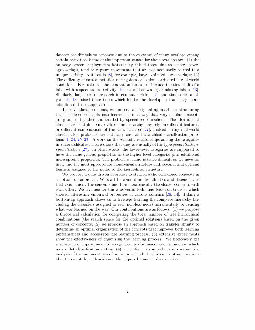
dataset are difficult to separate due to the existence of many overlaps amongcertain activities. Some of the important causes for these overlaps are: (1) theon-body sensors deployments featured by this dataset, due to sensors cover-age overlaps, tend to capture movements that are not necessarily related to aunique activity. Authors in [8], for example, have exhibited such overlaps; (2)The difficulty of data annotation during data collection conducted in real-worldconditions. For instance, the annotation issues can include the time-shift of alabel with respect to the activity [19], as well as wrong or missing labels [13].Similarly, long lines of research in computer vision [20] and time-series anal-ysis [19, 13] raised these issues which hinder the development and large-scaleadoption of these applications.

To solve these problems, we propose an original approach for structuringthe considered concepts into hierarchies in a way that very similar conceptsare grouped together and tackled by specialized classifiers. The idea is thatclassifications at different levels of the hierarchy may rely on different features,or different combinations of the same features [27]. Indeed, many real-worldclassification problems are naturally cast as hierarchical classification prob-lems [1, 24, 25, 27]. A work on the semantic relationships among the categoriesin a hierarchical structure shows that they are usually of the type generalization-specialization [27]. In other words, the lower-level categories are supposed tohave the same general properties as the higher-level categories plus additionalmore specific properties. The problem at hand is twice difficult as we have to,first, find the most appropriate hierarchical structure and, second, find optimallearners assigned to the nodes of the hierarchical structure.

We propose a data-driven approach to structure the considered concepts ina bottom-up approach. We start by computing the affinities and dependenciesthat exist among the concepts and fuse hierarchically the closest concepts witheach other. We leverage for this a powerful technique based on transfer whichshowed interesting empirical properties in various domains [26, 14]. Taking abottom-up approach allows us to leverage learning the complete hierarchy (in-cluding the classifiers assigned to each non-leaf node) incrementally by reusingwhat was learned on the way. Our contributions are as follows: (1) we proposea theoretical calculation for computing the total number of tree hierarchicalcombinations (the search space for the optimal solution) based on the givennumber of concepts; (2) we propose an approach based on transfer affinity todetermine an optimal organization of the concepts that improves both learningperformances and accelerates the learning process; (3) extensive experimentsshow the effectiveness of organizing the learning process. We noticeably geta substantial improvement of recognition performances over a baseline whichuses a flat classification setting; (4) we perform a comprehensive comparativeanalysis of the various stages of our approach which raises interesting questionsabout concept dependencies and the required amount of supervision.

2

2. Problem Statement

In this section, we briefly review the problem of hierarchical structuringof the concepts in terms of formulation and background. We then provide acomplexity analysis of the problem size and its search space.

2.1. Problem Formulation and Background

Let X ⊂ Rn be the inputs vector 1 and let C be the set of atomic concepts(or labels) to learn. The main idea of this paper comes from the fact that theconcepts to be learned are not totally independent, thus grouping some conceptsto learn them against the others using implicit biases considerably improves thequality of learning for each concept. The main problem is to find the beststructure of concepts groups to be learned in order to optimize the learning ofeach atomic concept. For this we follow the three dimensions setting definedin [10], and we consider: (1) single-label classification as opposed to multi-labelclassification; (2) the type of hierarchy (or structure) to be trees as opposed todirected acyclic graphs; (3) instances that have to be classified into leafs, i.e.mandatory leaf node prediction [17], as opposed to the setting where instancescan be classified into any node of the hierarchy (early stopping).

A tree hierarchy organizes the class labels into a tree-like structure to rep-resent a kind of ”IS-A” relationship between labels. Specifically, [10] points outthat the properties of the ”IS-A” relationship can be described as asymmetry,anti-reflexivity and transitivity [17]. We define a tree as a pair (C,≺), where Cis the set of class labels and ”≺” denotes the ”IS-A” relationship.

Let {(x1, c1), . . . , (xN , cN )} i.i.d.∼ X,C be a set of training examples, whereX and C are two random variables taking values in X × C, respectively. Eachxk ∈ X and each ck ∈ C. Our goal is to learn a classification function f : X −→ Cthat attains a small classification error. In this paper, we associate each nodei with a classifier Mi, and focus on classifiers f(x) that are parameterized byM1, . . . ,Mm through the following recursive procedure [27] (check Fig. 2):

f(x) =

initialize i := 0

while (Child(i) is not empty) i := argmaxj∈Child(i) Mj(x)

return i %Child(i) is the set of children for the node i

(1)

In the case of the SHL dataset, for instance, learning train and subway or car andbus before learning each concept alone gives better results. As an advantage,considering these classes paired together as opposed to the flat classificationsetting leads to significant degradation of recognition performances as demon-strated in some works around the SHL dataset [23]. In contrast, organizing the

1In our case, we select several body-motion modalities to be included in our experiments,among the 16 input modalities of the original dataset: accelerometer, gyroscope, etc. Segmen-tation and processing details are detailed in experimental part.

3

various concepts into a tree-like structure, inspired by domain expertise, demon-strated significant gains in terms of recognition performances in the context ofthe SHL challenge [12] and activity recognition in general [15, 16].

Designing such structures is of utmost importance but hard because it in-volves optimizing the structure as well as learning the weights of the classifiersattached to the nodes of that structure (see Sec. 2.2). Our goal is then to deter-mine an optimal structure of classes that can facilitate (improve and accelerate)learning of the whole concepts.

2.2. Search Space Size: Complexity Analysis

A naive approach is to generate the lattice structure of concepts groups andto choose the tree hierarchies which give the best accuracy of atomic concepts.In practice, this is not doable because of the exponential (in the number of leafnodes) number of possible trees. We propose a recurrence relation involvingbinomial coefficients for calculating the total number of tree hierarchies for Kdifferent concepts (class labels).

Example 1. Assume we have 3 various concepts, and we are interested incounting the total number of hierarchies for classifying these concepts. We con-sider that we have three classes namely c1, c2 and c3, there exist 4 different treehierarchies for learning the classification problem as following: (1) (c1c2c3) thetree has one level and the learning process takes one step. Three concepts arelearned while each concept is learned separately from the others (flat classifica-tion), (2) ((c1c2)c3) the tree has two levels and the learning process takes twosteps: at the first level, it learns two concepts (atomic c3 and two atomics c1and c2 together). At the second level it learns separately the two joined conceptsc1 and c2 of the first level, etc and (3) (c1(c2 c3)) and (4) ((c1c3)c2).

Theorem 1. Let L(K) be the total number of trees for the given K number ofconcepts. The total number of trees for K + 1 concepts satisfies the followingrecurrence relation: L(K+1) =

(KK−1

)L(K)L(1)+2

∑K−2i=0

(Ki

)L(i+1)L(K−i).

Proof 1. It can be explained by observing that, for K + 1 concepts containingK existed concepts c1, · · · cK and a new added concept γ, we can produce thefirst level trees combinations as below. Notice that each atomic element o canbe one of the c1, · · · cK concepts. In order to compute the total number of treescombinations, we show what is the number of tree combinations by assigning theK concepts to each item:

• (γ(

Kconcepts︷ ︸︸ ︷o · · · o )): the number of trees combinations by taking the concept

labels into the account are:(K0

)L(1)×2×L(K); the reason for multiplying

the number of trees combinations for K concepts to 2 is because while theleft side contains an atomic γ concept, there are two choices for the rightside of the tree in the first level: either we compute the total number of trees

4

for K concepts from the first level or we keep the first level as a

Kconcepts︷ ︸︸ ︷o · · · o

atomics and keep all K concepts together, then continue the number of Ktrees combinations from the second level of the tree.

• ((γo)(

K−1concepts︷ ︸︸ ︷o · · · o )): similar to the previous part we have

(K1

)L(2) × 2 ×

L(K−1) trees combinations by taking the concepts labels into the account.(K1

)indicates the number of combinations for choosing a concept from the

K concept and put it with the new concept separately. While L(2) is thenumber of trees combinations for the left side of tree separated with thenew concept γ.

• ((γoo)(

K−2concepts︷ ︸︸ ︷o · · · o )), · · ·

• ((γ

K−1concepts︷ ︸︸ ︷o · · · o )o):

(KK−1

)L(K)L(1) in this special part, we follow the same

formula except the single concept in the right side has only one possiblecombination in the first level equal to L(1).

All in all, the sum of these items calculates the total number of tree hierarchiesfor K + 1 concepts.

The first few number of total number of trees combinations for 1, 2, 3, 4, 5, 6,7, 8, 9, 10, · · · concepts are: 1 , 1, 4, 26, 236, 2752, 39208, 660032, 12818912,282137824, · · · . In the case of the SHL dataset that we use in the empiricalevaluation, we have 8 different concepts and thus, the number of different typesof hierarchies for this case is L(8) = 660, 032.

3. Proposed Approach

Our goals are to: (i) organize the considered concepts into hierarchies suchthat the learning process accounts for the dependencies existed among theseconcepts; (ii) characterize optimal classifiers that are associated to each non-leaf node of the hierarchies. Structuring the concepts can be performed usingtwo different approaches: a top-down approach where we seek to decomposethe learning process; and a bottom-up approach where the specialized modelsare grouped together based on their affinities. Our approach takes the latterdirection and constructs hierarchies based on the similarities between concepts.This is because, an hierarchical approach as a bottom-up method is efficient inthe case of high volume SHL data-sets. In this section, we detail the differentparts of our approach which are illustrated in Fig. 1. In the rest of this section,we introduce the three stages of our approach in detail: Concept similarityanalysis, Hierarchy derivation, and Hierarchy refinement.

5

1

2 3 4

5 6 7 8

1

2

3

4

5

6

7

8

7

86

5

43

2 1

3rd order

2nd order

...

Source Concept Encoder(e.g. 1:Still)

Target Concept Decoder(e.g. 6:Bus)

Concepts

Figure 1: Our solution involves several repetitions of 3 main steps: (1) Concept simi-larity analysis: encoders are trained to output, for each source concept, an appropriaterepresentation which is then fine-tuned to serve target concepts. Affinity scores aredepicted by the arrows between concepts (the thicker the arrow, the higher the affin-ity score). (2) Hierarchy derivation: based on the obtained affinity scores, a hierarchyis derived using an agglomerate approach. (3) Hierarchy refinement: each non-leafnode of the derived hierarchy is assigned with a model that encompasses the appro-priate representation as well as an ERM which is optimized to separate the consideredconcepts.

3.1. Concept Similarity (Affinity) Analysis

In our bottom-up approach we leverage transferability and dependencyamong concepts as a measure of similarity. Besides the nice empirical propertiesof this measure (explained in the Properties paragraph below), the argumentbehind it is to reuse what has been learned so far at the lower levels of thehierarchies. Indeed, we leverage the models that we learned during this stepand use them with few additional adjustments in the final hierarchical learningsetting.

Transfer-based affinity. Given the set of concepts C, we compute during thisstep an affinity matrix that captures the notion of transferability and similarity,among the concepts. For this, we first compute for each concept ci ∈ C an en-coder f ciθ (parameterized by θ) that learns to map the ci labeled inputs, to Zci .Learning the encoder’s parameters consists in minimizing the reconstruction er-ror, satisfying the following optimization [22]: argminθ,θ′ Ex,c∼X,C|c=ciL(gciθ′ (f

ciθ (x)), x),

where gciθ′ is a decoder (parameterized by θ′) which maps back the learned rep-resentation into the original inputs space. We propose to leverage the learnedencoder, for a given concept ci, to compute affinities with other concepts via fine-tuning of the learned representation. Precisely, we fine-tune the encoder fθci toaccount for a target concept cj ∈ C. This process consists, similarly, in minimiz-ing the reconstruction error, however rather than using the decoder gciθ′ learnedabove, we design a genuine decoder g

cjθ′ that we learn from the scratch. The cor-

responding objective function is argminθ,θ′ Ex,c∼X,C|c=cjL(gcjθ′ (f ciθ (x)), x). We

use the performance of this step as a similarity score from ci to cj which wedenote by pci−→cj ∈ [0, 1]. We refer to the number of examples belonging tothe concept cj used during fine-tuning as the supervision budget, denoted as b,which is used to index a given measure of similarity. It allows us to have anadditional indicator as to the similarity between the considered concepts. The

6

final similarity score is computed asα·pci−→cj

+β·bα+β . We set α and β to be equal

to 12 .

Properties. In many applications, e.g. computer-vision [26] and natural lan-guage processing [14], several variants of the transfer-based similarity measurehave been shown empirically to improve (i) the quality of transferred models(wins against fully supervised models), (ii) the gains, i.e. win rate againsta network trained from scratch using the same training data as transfer net-works’, and more importantly (iii) the universality of the resulting structure.Indeed, the affinities based on transferability are stable despite the variationsof a big corpus of hyperparameters. We provide empirical evidence (Sec. 6.2) ofthe appropriateness of the transfer-based affinity measure for the separabilityof the similar concepts and the difficulty to separate concepts that exhibit lowsimilarity scores.

3.2. Hierarchy Derivation

Given the set of affinity scores obtained previously, we derive the most appro-priate hierarchy, following an agglomerative clustering method combined withsome additional constraints. The agglomerative clustering method proceeds bya series of successive fusions of the concepts into groups and results in a struc-ture represented by a two-dimensional diagram known as a dendrogram. Itworks by (1) forming groups of concepts that are close enough and (2) updatingthe affinity scores based on the newly formed groups. This process is definedby the recurrence formula proposed by [11]. If defines a distance between agroup of concepts (k) and a group formed by fusing i and j groups (ij) asdk(ij) = αidki + αjdkj + βdij + γ|dki − dkj |, where dij is the distance betweentwo groups i and j. By varying the parameter values αi, αj , β, and γ, we expectto get clustering schemes with various characteristics.

In addition to the above updating process, we propose additional constraintsto refine further the hierarchy derivation stage. Given the dendrogram producedby the agglomerative method above, we define an affinity threshold τ such thatif the distance at a given node is dij ≥ τ , then we merge the nodes to forma unique subtree. In addition, as we keep track of the quantities of data usedto train and fine-tune the encoders during the transfer-based affinity analysisstage, this indicator is exploited to inform us as to which nodes to merge. Let Tbe the derived hierarchy (tree) and let t indexes the non-leaf or internal nodes.The leafs of the hierarchy correspond to the considered concepts. For any non-leaf node t, we associate a modelMt that encompasses (1) an encoder (denotedin the following simply by Zt in order to focus on the representation) that mapsinputs X to representations Zt and (2) an ERM (Empirical Risk Minimizer) [21]ft (such as support vector machines SVMs) that outputs decision boundariesbased on the representations produced by the encoder.

3.3. Hierarchy Refinement

After explaining the hierarchy derivation process, we will discuss: (1) whichrepresentations are used in each individual model; and (2) how each individ-

7

ual model (including the representation and the ERM weights) is adjusted toaccount for both the local errors and also those of the hierarchy as a whole.

Which representations to use?. The question discussed here is related to theencoders to be used in each non-leaf node. For any non-leaf node t we distinguishtwo cases: (i) all its children are leafs; (ii) it has at least one non-leaf node. Inthe first case, the final considered ERM representation, associated with thenon-leaf node, is the representation learned in the concept affinity analysis step(first-order transfer-based affinity). In the second case, we can either fuse thenodes (for example, in a case of classification between 3 concepts, we get all 3together rather than, first {1} vs. {2,3}, then {2} vs. {3}), or keep them asthey are and leverage the affinities based on higher-order transfer where, ratherthan accounting for a unique target concept, the representation is then fine-tuned. Fig. 2 illustrates how transfers are performed between non-leaf nodesmodels. We index the models with the encoder M[Zi]. In the case of higher-order transfer, the models are indexed using all concepts involved in the transfer,i.e. M[Zi,j,...].

M[zj ]

cj ck

M[zi,j ]

ci

(a)

cj ck

M[zi,j,k]

ci

(b)

M[zj ]

cj ck

M[zi,j ]

M[zj ]

...

(c)

Figure 2: Transfers are performed between non-leaf nodes models. The hierarchy in (a)can be kept as they are merged to form the hierarchy in (b). (b): a high-order transferbetween the concepts ci, cj , and ck is performed. (c): no transfers can be made.

Adjusting models weights. Classifiers are trained to output a hypothesis basedon the most appropriate representations learned earlier. Given the encoder(representation) assigned to any non-leaf node t, we select a classifier f :=argminf∈H R(f,Zt) where R(f,Zt) := 1

M

∑x,c∼X,C|c∈Child(t) Ez∼Zt|x[L(c, f(z))]

and H is the hypothesis space. Models are adjusted to account for local errorsas well as for global errors related to the hierarchy as a whole. In the first case,the loss is defined as the traditional hinge loss used in SVMs which is intendedto adjust the weights of the classifiers that have only children leaves. In thesecond case, we use a loss that encourages the models to leverage orthogonalrepresentations (between children and parent nodes) [27].

4. Experiments and Results

Empirical evaluation of our approach are performed on three steps: we eval-uate classification performances in the hierarchical setting (Sec. 6.1); then, we

8

evaluate the transfer-based affinity analysis step and the properties related tothe separability of the considered concepts (Sec. 6.2); finally, we evaluate thederived hierarchies in terms of stability, performance, and agreement with theircounterparts defined by domain experts (Sec. 6.3) 2. Training details can befound in 5 and evaluation metrics are detailed in 6.

SHL dataset [7]. It is a highly versatile and precisely annotated dataset ded-icated to mobility-related human activity recognition. In contrast to relatedrepresentative datasets like [2], the SHL dataset (26.43 GB) provides , simul-taneously, multimodal and multilocation locomotion data recorded in real-lifesettings. Among the 16 modalities of the original dataset, we select the body-motion modalities including: accelerometer, gyroscope, magnetometer, linearacceleration, orientation, gravity, and ambient pressure. This makes the dataset suitable for a wide range of applications and in particular transportationrecognition concerned with this paper. From the 8 primary categories of trans-portation, we are selected: 1:Still, 2:Walk, 3:Run, 4:Bike, 5:Car, 6:Bus, 7:Train,and 8:Subway (Tube).

5. Training Details

We use Tensorflow for building the encoders/decoders. We construct en-coders by stacking Conv1d/ReLU/MaxPool blocks. These blocks are followedby a Fully Connected/ReLU layers. Encoders performance estimation is basedon the validation loss and is framed as a sequence classification problem. Asa preprocessing step, annotated input streams from the huge SHL dataset aresegmented into sequences of 6000 samples which correspond to a duration of 1min. given a sampling rate of 100 Hz. For weight optimization, we use stochasticgradient descent with Nesterov momentum of 0.9 and a learning-rate of 0.1 fora minimum of 12 epochs (we stop training if there is no improvement). Weightdecay is set to 0.0001. Furthermore, to make the neural networks more stable,we use batch normalization on top of each convolutional layer. We use SVMsas our ERMs in the derived hierarchies.

6. Evaluation Metrics

In hierarchical classification settings, the hierarchical structure is importantand should be taken into account during model evaluation [17]. Various mea-sures that account for the hierarchical structure of the learning process havebeen studied in the literature. They can be categorized into: distance-based;depth-dependent; semantics-based; and hierarchy-based measures. Each oneis displaying advantages and disadvantages depending on the characteristics of

2Software package and code to reproduce empirical results are publicly available at https://github.com/sensor-rich/hierarchicalSHL

9

the considered structure [5]. In our experiments, we use the H-loss, a hierarchy-based measure defined in [3]. This measure captures the intuition that ”when-ever a classification mistake is made on a node of the taxonomy, then no lossshould be charged for any additional mistake occurring in the sub-tree of thatnode.” `H(y, y) =

∑Ni=1{yi 6= yi ∧ yj = yj , j ∈ Anc(i)}, where y = (y1, · · · yN )

is the predicted labels, y = (y1, · · · yN ) is the true labels, and Anc(i) is the setof ancestors for the node i.

6.1. Evaluation of the Hierarchical Classification Performances

In these experiments, we evaluate the flat classification setting using neuralnetworks which constitute our baseline for the rest of the empirical evaluations.To compare our baseline with the hierarchical models, we make sure to get thesame complexity, i.e. comparable number of parameters as the largest hierar-chies including the weights of the encoders and those of the ERMs. We also useBayesian optimization based on Gaussian processes as surrogate models to selectthe optimal hyperparameters of the baseline model [18, 9]. More details aboutthe baseline and its hyperparameters are available in the code repository [9].

Per-node performances. Fig. 3 shows the resulting per-node performances, i.e.how accurately the models associated with the non-leaf nodes can predict thecorrect subcategory averaged over the entire derived hierarchies. The nodesare ranked according to the obtained per-node performance (top 10 nodes areshown) and accompanied by their appearance frequency. It is worth noticingthat the concept 1:still learned alone against the rest of the concepts (firstbar) achieves the highest gains in terms of recognition performances while theappearance frequency of this learning configuration is high (more than 60 times).We see also that the concepts 4:bike, 5:car, and 6:bus grouped together (5th bar)occur very often in the derived hierarchies (80 times) which is accompanied byfairly significant performance gains (5.09±0.3%). At the same time, as expected,we see that the appearance frequency gets into a plateau starting from the 6thbar (which lasts after the 10th bar). This suggests that the most influentialnodes are often exhibited by our approach.

Per-concept performances. We further ensure that the performance improve-ments we get at the node levels are reflected at the concept level. Experimentalresults show the recognition performances of each concept, averaged over thewhole hierarchies derived using our proposed approach. We indeed observe thatthere are significant improvements for each individual concept over the baseline(flat classification setting). We observe that again 1:still has the highest classi-fication rate (72.32± 3.45%) and an improvement of 5 points over the baseline.Concept 6:bus also exhibits a roughly similar trend. On the other hand, con-cept 7:train has the least gains (64.43±4.45%) with no significant improvementover the baseline. Concept 8:subway exhibits the same behavior suggesting thatthere are undesirable effects that stem from the definition of these two concepts.

10

0

2

4

6

8

0

20

40

60

80

1 2 3 4 5 6 7 8 9 10

Perf. gainsAppear. freq.

Per

form

ance

gain

s(%

)

Nodes

Ap

pea

ran

cefr

equ

ency

(a)

Cla

ssifi

cati

onp

erfo

rman

ces

(%)

HierarchicalBaseline

1:still 2:walk 3:run 4:bike 5:car 6:bus 7:train 8:subway

85

80

75

70

65

60

(b)

Figure 3: (a) Per-node performance gains, averaged over the entire derived architectures(similar nodes are grouped and their performances are averaged). The appearance frequencyof the nodes is also illustrated. Each bar represents the gained accuracy of each node in ourhierarchical approach. For example, the 8th bar corresponds to the concepts 2:walk-3:run-4:bike grouped together. (b) Recognition performances of each individual concept, averagedover the entire derived hierarchies. For reference, the recognition performances of the baselinemodel are also shown.

11

M[zi]

ci cj

(a) (b)

Init

ial

tran

sfer

-bas

edaffi

nit

ysc

ores

Supervision budget (# learning examples)200 300 400 500

0.2

0.4

0.6

0.8

(c)

Figure 4: (a) Non-leaf node grouping concepts ci and cj . (b) Decision boundaries generatedby the ERM of the non-leaf node using an encoder (representation) fine-tuned to account for(top) the case where ci and cj are dissimilar (low-affinity score) and (bottom) the case whereci and cj are similar (high-affinity score). (c) Decision boundaries obtained by SVM-basedclassifiers trained on the representations Zt as a function of the distance between the concepts(y-axis) and the supervision budget (x-axis).

6.2. Evaluation of the Affinity Analysis Stage

These experiments evaluate the proposed transfer-based affinity measure.We assess, the separability of the concepts depending on their similarity score(for both the transfer-affinity and supervision budget) and the learned repre-sentation.

Appropriateness of the Transfer-based Affinity Measure. We reviewed above thenice properties of the transfer-based measure especially the universality andstability of the resulting affinity structure. The question that arises is relatedto the separability of the concepts that are grouped together. Are the obtainedrepresentations, are optimal for the final ERMs used for the classification? Thisis what we investigate here. Fig. 4b shows the decision boundaries generatedby the considered ERMs which are provided with the learned representationsof two concepts. The first case (top right), exhibits a low-affinity score, andthe second case (bottom right) shows a high-affinity score. In the first case, theboundaries are unable to separate the two concepts while it gets a fairly distinctfrontier.

Impact on the ERMs’ Decision Boundaries. We train different models withvarious learned representations in order to investigate the effect of the initial

12

affinities (obtained solely with a set of 100 learning examples) and the supervi-sion budget (additional learning examples used to fine-tune the obtained repre-sentation) on the classification performances of the ERMs associated with thenon-leaf nodes of our hierarchies. Fig. 4c shows the decision boundaries gen-erated by various models as a function of the distance between the concepts(y-axis) and the supervision budget (x-axis). Increasing the supervision budgetto some larger extents (more than ∼ 300 examples) results in a substantial de-crease in classification performances of the ERMs. This suggests that, althoughour initial affinity scores are decisive (e.g. 0.8), the supervision budget is tightlylinked to generalization. This shows that a trade-off (controlled by the super-vision budget) between separability and initial affinities arises when we seek togroup concepts together. In other words, the important question is whether toincrease the supervision budget indefinitely (in the limits of available learningexamples) in order to find the most appropriate concepts to fuse with, whileexpecting good separability.

6.3. Universality and Stability

We demonstrated in the previous section the appropriateness of the transfer-based affinity measure to provide distance between concepts as well as the exis-tence of a trade-off between concepts separability and their initial affinities. Herewe evaluate the universality of the derived hierarchies as well as their stabil-ity during adaptation with respect to our hyperparameters (affinity thresholdand supervision budget). We compare the derived hierarchies with their domainexperts-defined counterparts, as well as those obtained via a random samplingprocess. Fig. 5 shows some of the hierarchies defined by the domain experts(first row) and sampled using the random sampling process. For example, thehierarchy depicted in Fig. 5d corresponds to a split between static (1:still, 5:car,6:bus, 7:train, 8:subway) and dynamic (2:walk, 3:run, 4:bike) activities. The dif-ference between the hierarchies depicted in Fig. 5a and 5b is related to 4:bikeactivity which is linked first to 2:walk and 3:run then to 5:car and 6:bus. Apossible interpretation is that in the first case, biking is considered as “on feet”activity while in the second case as “on wheels” activity. What we observed isthat the derived hierarchies tend to converge towards the expert-defined ones.

Method Agree. perf. avg.± std.

Expertise - 72.32±0.17Random 0.32 48.17±5.76Proposed 0.77 75.92±1.13

Table 1: Summary of the recognition performances obtained with our proposed approachcompared to randomly sampled and expert-defined hierarchies.

We compare the derived hierarchies in terms of their level of agreement. Weuse for this assessment, the Cohen’s kappa coefficient [4] which measures theagreement between two raters. The first column of Table 1 provides the obtained

13

1

2 3 4 5 6 7 8

(a)

1

2 3 4 5 6 7 8

(b)

1

2 3 4

5 6 7 8

(c)

1

2 3 4 5 6 7 8

(d)

Figure 5: Examples of hierarchies: (a) defined via domain expertise, (b-c) derived using ourapproach, and (d) randomly sampled. Concepts 1—8 from left to right.

coefficients. We also compare the average recognition performance of the derivedhierarchies (second column of Table 1). In terms of stability, as we vary thedesign choices (hyperparameters), defined in our approach, we found that theaffinity threshold has a substantial impact on our results with many adjustmentsinvolved (12 hierarchy adjustments on avg.) whereas the supervision budget hasa slight effect, which confirms the observations in Sec. 6.2.

7. Conclusion and Future Work

This paper proposes an approach for organizing the learning process of de-pendent concepts in the case of human activity recognition. We first determinea suitable structure for the concepts according to a transfer affinity-based mea-sure. We then characterize optimal representations and classifiers which arethen refined to account for both local and global errors. We provide theoreticalbounds for the problem and empirically show that using our approach we areable to improve the performances and robustness of activity recognition mod-els over a flat classification baseline. In addition to supporting the necessityof organizing concepts learning, our experiments raise interesting questions forfuture work. Noticeably, Sec. 6.2 asks what is the optimal amount of super-vision for deriving the hierarchies. Another future work is to study differentapproaches for searching and exploring the search space of different hierarchicaltypes (lattices, etc.).

References

[1] Cai, L., Hofmann, T.: Hierarchical document categorization with supportvector machines. In: CIKM. pp. 78–87 (2004)

[2] Carpineti, C., et al.: Custom dual transportation mode detection by smart-phone devices exploiting sensor diversity. In: PerCom wksh. pp. 367–372.IEEE (2018)

14

[3] Cesa-Bianchi, N., Gentile, C., Zaniboni, L.: Incremental algorithms forhierarchical classification. JMLR 7(Jan), 31–54 (2006)

[4] Cohen, J.: A coefficient of agreement for nominal scales. Educational andpsychological measurement 20(1), 37–46 (1960)

[5] Costa, E., Lorena, A., Carvalho, A., Freitas, A.: A review of performanceevaluation measures for hierarchical classifiers. In: Evaluation Methods formachine Learning II: papers from the AAAI-2007 Workshop. pp. 1–6 (2007)

[6] Essaidi, M., Osmani, A., Rouveirol, C.: Learning dependent-concepts inilp: Application to model-driven data warehouses. In: ILP, pp. 151–172(2015)

[7] Gjoreski, H., et al.: The university of sussex-huawei locomotion and trans-portation dataset for multimodal analytics with mobile devices. IEEE Ac-cess (2018)

[8] Hamidi, M., Osmani, A.: Data generation process modeling for activityrecognition. In: ECML-PKDD. Springer (2020)

[9] Hamidi, M., Osmani, A., Alizadeh, P.: A multi-view architecture for theshl challenge. In: UbiComp/ISWC Adjunct. p. 317–322 (2020)

[10] Kosmopoulos, A., Partalas, I., Gaussier, E., Paliouras, G., Androutsopou-los, I.: Evaluation measures for hierarchical classification: a unified viewand novel approaches. Data Mining and Knowledge Discovery 29(3), 820–865 (2015)

[11] Lance, G.N., Williams, W.T.: A general theory of classificatory sortingstrategies: 1. hierarchical systems. The computer journal 9(4), 373–380(1967)

[12] Nakamura, Y., et al.: Multi-stage activity inference for locomotion andtransportation analytics of mobile users. In: UbiComp/ISWC. pp. 1579–1588 (2018)

[13] Nguyen-Dinh, L.V., Calatroni, A., Troster, G.: Robust online gesturerecognition with crowdsourced annotations. JMLR 15(1), 3187–3220 (2014)

[14] Peters, M.E., Ruder, S., Smith, N.A.: To tune or not to tune? adapting pre-trained representations to diverse tasks. arXiv preprint arXiv:1903.05987(2019)

[15] Samie, F., Bauer, L., Henkel, J.: Hierarchical classification for constrainediot devices: A case study on human activity recognition. IEEE IoT Journal(2020)

[16] Scheurer, S., et al.: Using domain knowledge for interpretable and compet-itive multi-class human activity recognition. Sensors 20(4), 1208 (2020)

15

[17] Silla, C.N., Freitas, A.A.: A survey of hierarchical classification acrossdifferent application domains. Data Mining and Knowledge Discovery 22(1-2), 31–72 (2011)

[18] Snoek, J., Larochelle, H., Adams, R.P.: Practical bayesian optimization ofmachine learning algorithms. In: NIPS. pp. 2951–2959 (2012)

[19] Stikic, M., Schiele, B.: Activity recognition from sparsely labeled datausing multi-instance learning. In: Int. Symposium on LoCA. pp. 156–173.Springer (2009)

[20] Taran, V., Gordienko, Y., Rokovyi, A., Alienin, O., Stirenko, S.: Impactof ground truth annotation quality on performance of semantic image seg-mentation of traffic conditions. In: ICCSEA. pp. 183–193. Springer (2019)

[21] Vapnik, V.: Principles of risk minimization for learning theory. In: NIPS(1992)

[22] Vincent, P., et al.: Stacked denoising autoencoders: Learning useful repre-sentations in a deep network with a local denoising criterion. JMLR 11(12)(2010)

[23] Wang, L., et al.: Summary of the sussex-huawei locomotion-transportationrecognition challenge. In: UbiComp/ISWC. pp. 1521–1530 (2018)

[24] Wehrmann, J., Cerri, R., Barros, R.: Hierarchical multi-label classificationnetworks. In: ICML. pp. 5075–5084 (2018)

[25] Yao, H., Wei, Y., Huang, J., Li, Z.: Hierarchically structured meta-learning.In: ICML. pp. 7045–7054 (2019)

[26] Zamir, A.R., Sax, A., Shen, W., Guibas, L.J., Malik, J., Savarese, S.:Taskonomy: Disentangling task transfer learning. In: CVPR. pp. 3712–3722 (2018)

[27] Zhou, D., Xiao, L., Wu, M.: Hierarchical classification via orthogonal trans-fer. In: ICML. pp. 801–808 (2011)

16