Aff Excel 2010

UNIVERSITY INFORMATION TECHNOLOGY TRAINING & DOCUMENTATION DEPARTMENT

DOING MORE WITH EXCEL 2010: AUTOMATING,

FORMULAS, AND FILTERS

University Information Technology Training & Documentation Department 2


Table of Contents The Workbook Environment .................................................................... 5

What is Excel? .................................................................................................. 5

Advanced Navigation ..................................................................................... 6

Moving Directly to a Specific Cell or Range .......................................................... 6 Locate Specific Cell Entries Anywhere on the Worksheet .................................... 7 Replacing Specific Cell Entries ............................................................................. 8

Transpose Feature ........................................................................................ 9

Macros ............................................................................................................ 11

Create a Custom Quick Access Toolbar Button for a Macro ............................... 17

Sorting Rows of Data ................................................................................... 19 Sorting by Multiple Criteria ........................................................................... 21

AutoFilter ......................................................................................................... 23

Using the Custom AutoFilter ............................................................................... 24

Referencing Cells in Formulas ..................................................................... 27 Relative and Absolute References ............................................................... 27 Referencing Cells Outside the Current Worksheet ...................................... 30

AutoSum ......................................................................................................... 35

Common Excel Error Values ........................................................................ 38 The Insert Function dialog box ..................................................................... 39

Using Functions .............................................................................................. 39

Using the CONCATENATE function ............................................................ 42 Converting Text to Columns ........................................................................ 45

Conditional formatting ..................................................................................... 48

Data Validation ................................................................................................ 53

Compatibility Checker ..................................................................................... 55

Changing the Page Setup ............................................................................... 56

Excel Function (F) Key Shortcuts ................................................................ 61

Tufts Computing & Communications Services Training & Documentation Department 5

THE WORKBOOK ENVIRONMENT

WHAT IS EXCEL? Excel is a software program included in Microsoft's Office package that runs on Windows and Apple Macintosh computer operating systems. It replaces yesteryear's columnar pad, pencil, and calculator by processing even the most complex calculations with ease. Excel users can create electronic worksheets, databases, three-dimensional charts and graphic images. In Excel data can easily be filtered, sorted, manipulated, and displayed in accessible formats. Throughout this session, the following topics will be covered:

Cell References

AutoSum

Functions

Macros

Sorting data

Filtering data

Range Names


ADVANCED NAVIGATION Worksheets can become cumbersome over time as they grow. Navigating with the mouse or the arrow keys can be tiresome and time consuming. To accommodate spreadsheet users who need to navigate through large volumes of data, Excel has built in a number of advanced navigation techniques. Excel also provides different ways to display specific ranges of data for easier viewing within a large spreadsheet.

MOVING DIRECTLY TO A SPECIFIC CELL OR RANGE Excel makes it very easy to go directly to a cell if you know the cell’s name, such as H45. You can also go to a range of cells by referencing the range of cell numbers, such as H45:R45, or by referencing the range name. A range name is a user friendly name that refers to a range of cells. It is much easier to remember a name than the cell references themselves. We will learn how to create range names later.

1. In the class files folder, open the file ExcelAFF.xlsx.

2. Select the first sheet tab Expenses.

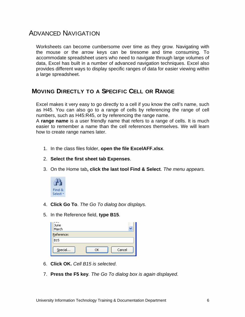
3. On the Home tab, click the last tool Find & Select. The menu appears.

4. Click Go To. The Go To dialog box displays.

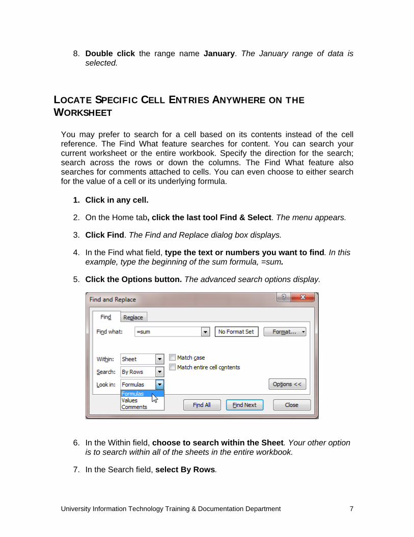
5. In the Reference field, type B15.

6. Click OK. Cell B15 is selected.

7. Press the F5 key. The Go To dialog box is again displayed.


8. Double click the range name January. The January range of data is selected.

LOCATE SPECIFIC CELL ENTRIES ANYWHERE ON THE WORKSHEET

You may prefer to search for a cell based on its contents instead of the cell reference. The Find What feature searches for content. You can search your current worksheet or the entire workbook. Specify the direction for the search; search across the rows or down the columns. The Find What feature also searches for comments attached to cells. You can even choose to either search for the value of a cell or its underlying formula.

1. Click in any cell.


3. Click Find. The Find and Replace dialog box displays.

4. In the Find what field, type the text or numbers you want to find. In this example, type the beginning of the sum formula, =sum.

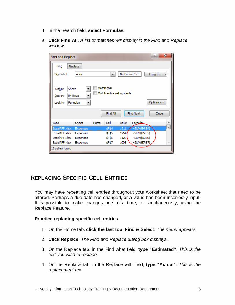
5. Click the Options button. The advanced search options display.

6. In the Within field, choose to search within the Sheet. Your other option is to search within all of the sheets in the entire workbook.

7. In the Search field, select By Rows.


8. In the Search field, select Formulas.

9. Click Find All. A list of matches will display in the Find and Replace window.

REPLACING SPECIFIC CELL ENTRIES

You may have repeating cell entries throughout your worksheet that need to be altered. Perhaps a due date has changed, or a value has been incorrectly input. It is possible to make changes one at a time, or simultaneously, using the Replace Feature. Practice replacing specific cell entries


2. Click Replace. The Find and Replace dialog box displays.

3. On the Replace tab, in the Find what field, type “Estimated”. This is the text you wish to replace.

4. On the Replace tab, in the Replace with field, type “Actual”. This is the replacement text.


5. Click the Find Next button. The first match of Estimated is found.

6. Click the Replace button. Estimated is replaced with Actual.

7. Click the Replace All button. The remaining four instances of Estimated are replaced with Actual.

8. Click Close.

TRANSPOSE FEATURE Transpose Rows to Columns or Columns to Rows There are times that you may design a spreadsheet, expending considerable time, only to come to the conclusion that your spreadsheet would be clearer if the columns and rows were reversed. Naturally you want your spreadsheet to be clearly designed, but re-doing it seems like a waste of time. Excel anticipates that this might happen to spreadsheet users, so it provides a Transpose Feature. Practice transposing the rows and columns in the Expenses sheet.

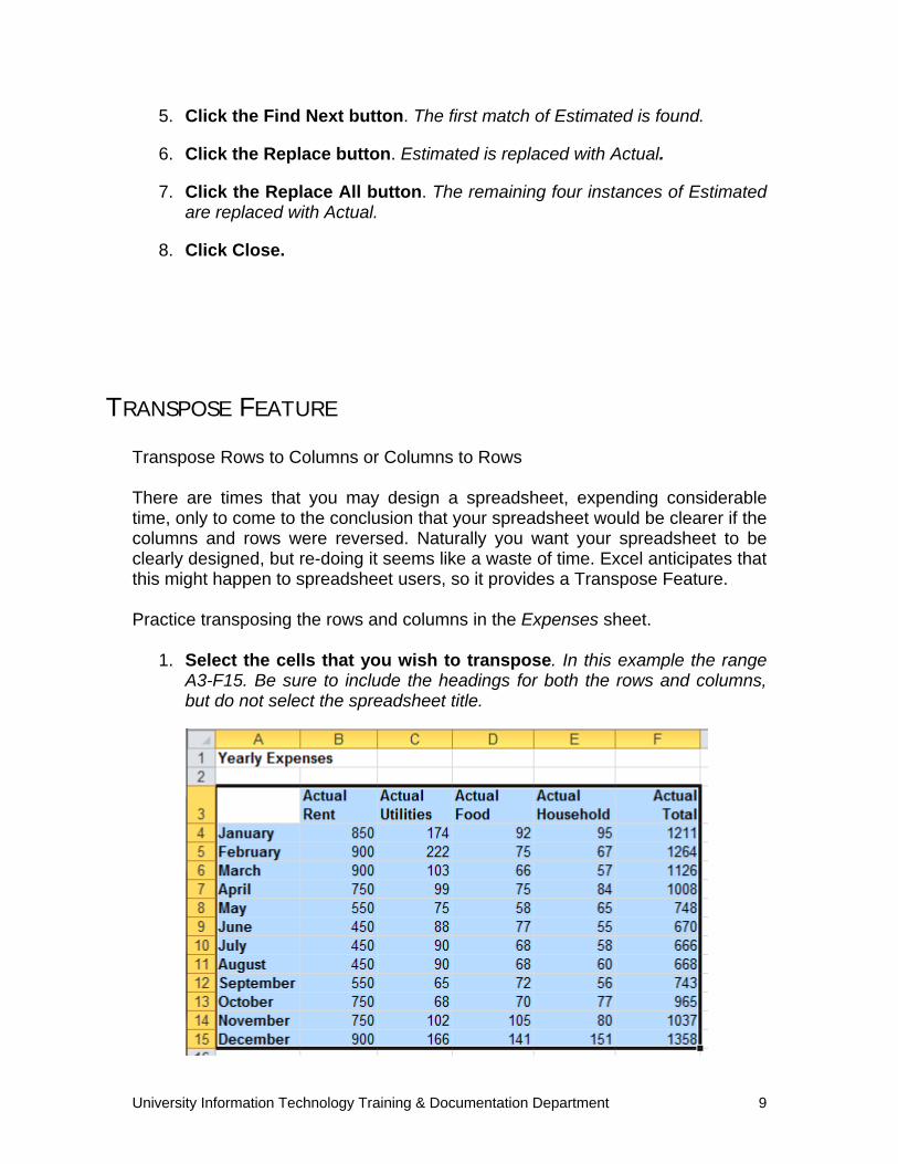
1. Select the cells that you wish to transpose. In this example the range A3-F15. Be sure to include the headings for both the rows and columns, but do not select the spreadsheet title.


2. On the Home tab, click the Copy tool (or copy using your favorite method).

The next step is to select the cell that will hold the upper left hand corner of the table.

3. Select cell A17. The new spreadsheet will be anchored here.

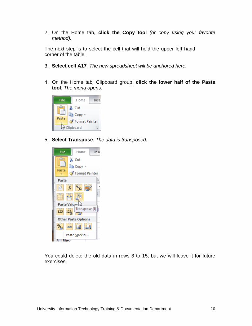
4. On the Home tab, Clipboard group, click the lower half of the Paste

tool. The menu opens.

5. Select Transpose. The data is transposed.

You could delete the old data in rows 3 to 15, but we will leave it for future exercises.


MACROS Macros are a series of commands that automate your work; you can create them to perform complex tasks or a simple task that you perform repeatedly. With macros, these tasks are performed at the touch of a button. Before recording a macro, you should plan your steps carefully. Review just what it is —step-by-step — that you wish to accomplish. To record and use a macro, two initial steps must be taken. First, the Developer tab must be visible. Generally, the Developer tab is not visible by default. Secondly, macros need to be enabled, as they are disabled by default (unless you are saving the file as a macro-enabled file: .xlsm). If the Developer tab is not available, follow these four steps to display it:

1. Click the File tab . The Backstage view displays.

2. On the left menu, select Options. The Excel Options dialog box displays.

3. In the Customize Ribbon category, in the right-hand pane, place a check in the Developer tab check box.

4. At the base of the window, click OK. The dialog box closes and the Developer tab displays on the Ribbon.

If you find that your Macro does not run, you may need to set the security level temporarily to enable all macros, which allows macros to run or execute.

To adjust the macro settings:

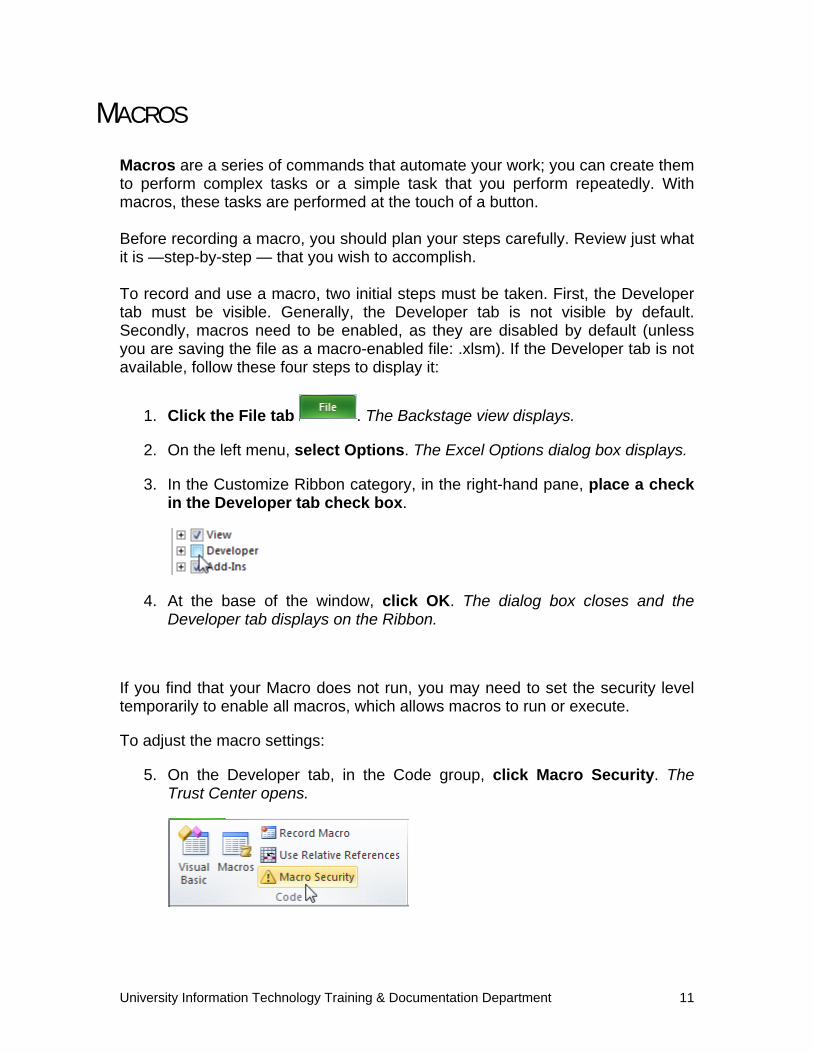
5. On the Developer tab, in the Code group, click Macro Security. The Trust Center opens.


6. Under Macro Settings, select the Enable all macros (not recommended, potentially dangerous code can run) option.

7. Click OK. The window closes and the macro security level is adjusted.

Macro for sorting by campus and creating new sheet We will create a basic macro that will sort and filter a list by campus, and then copy and paste the filtered results into a new sheet.

1. On the Developer tab, in the Code group, click Record Macro. The Record Macro dialog box is displayed.


The Record Macro Dialog Box requests 4 pieces of information: the name you wish to give your macro; the short cut key—if any—you wish to use; the place where you want to store your macro; and a macro description. Select a name for your macro that reflects the macro’s actions. You may not use spaces when naming your macro. If you need a space, use an underscore. Excel also prohibits you from using symbols and punctuation marks. Macro names are not case sensitive.

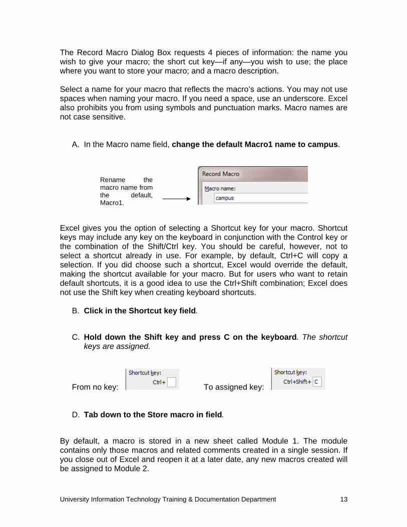
A. In the Macro name field, change the default Macro1 name to campus.

Excel gives you the option of selecting a Shortcut key for your macro. Shortcut keys may include any key on the keyboard in conjunction with the Control key or the combination of the Shift/Ctrl key. You should be careful, however, not to select a shortcut already in use. For example, by default, Ctrl+C will copy a selection. If you did choose such a shortcut, Excel would override the default, making the shortcut available for your macro. But for users who want to retain default shortcuts, it is a good idea to use the Ctrl+Shift combination; Excel does not use the Shift key when creating keyboard shortcuts.

B. Click in the Shortcut key field.

C. Hold down the Shift key and press C on the keyboard. The shortcut

keys are assigned.

From no key: To assigned key: D. Tab down to the Store macro in field.

By default, a macro is stored in a new sheet called Module 1. The module contains only those macros and related comments created in a single session. If you close out of Excel and reopen it at a later date, any new macros created will be assigned to Module 2.

Rename the macro name from the default, Macro1.


Macros created and stored within a workbook are only available for use in that workbook. You may also store the macro in another workbook. If you want to utilize that macro in another workbook, meaning that this macro will be available anytime you are using Excel, you need to store it in your Personal Macro workbook.

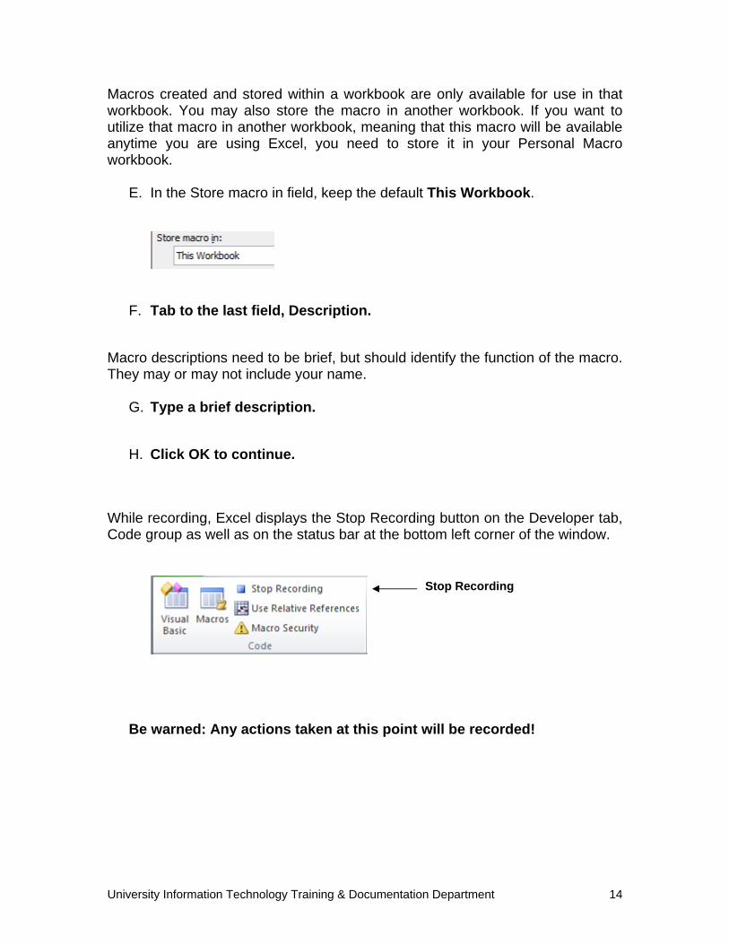
E. In the Store macro in field, keep the default This Workbook.

F. Tab to the last field, Description.

Macro descriptions need to be brief, but should identify the function of the macro. They may or may not include your name.

G. Type a brief description.

H. Click OK to continue.

While recording, Excel displays the Stop Recording button on the Developer tab, Code group as well as on the status bar at the bottom left corner of the window.

Be warned: Any actions taken at this point will be recorded!

Stop Recording


To record the steps of your macro:

A. Click anywhere in the data (in the table).

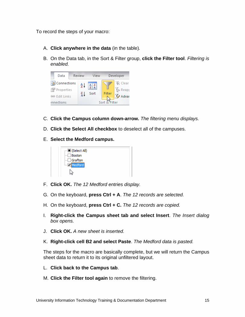
B. On the Data tab, in the Sort & Filter group, click the Filter tool. Filtering is enabled.

C. Click the Campus column down-arrow. The filtering menu displays.

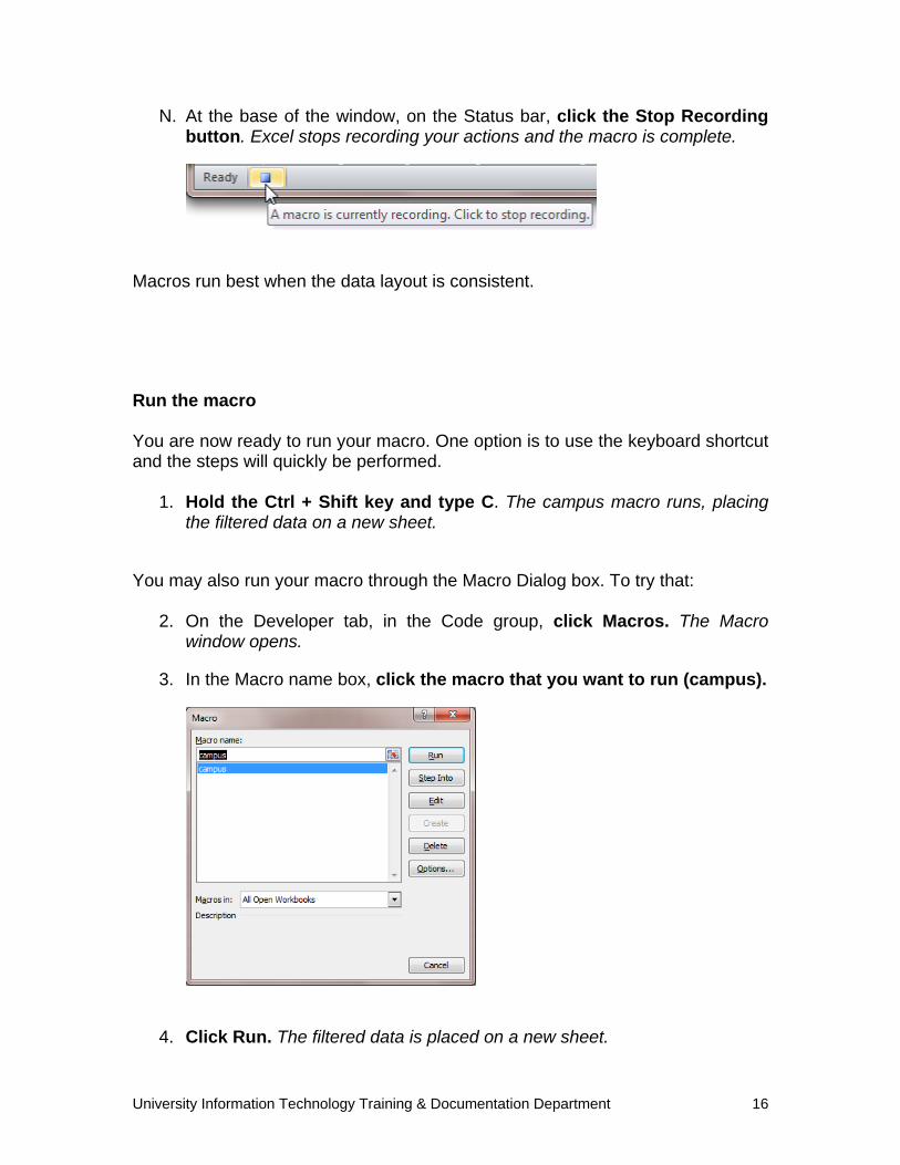
D. Click the Select All checkbox to deselect all of the campuses.

E. Select the Medford campus.

F. Click OK. The 12 Medford entries display.

G. On the keyboard, press Ctrl + A. The 12 records are selected.

H. On the keyboard, press Ctrl + C. The 12 records are copied.

I. Right-click the Campus sheet tab and select Insert. The Insert dialog box opens.

J. Click OK. A new sheet is inserted.

K. Right-click cell B2 and select Paste. The Medford data is pasted.

The steps for the macro are basically complete, but we will return the Campus sheet data to return it to its original unfiltered layout.

L. Click back to the Campus tab.

M. Click the Filter tool again to remove the filtering.


N. At the base of the window, on the Status bar, click the Stop Recording button. Excel stops recording your actions and the macro is complete.

Macros run best when the data layout is consistent.

Run the macro You are now ready to run your macro. One option is to use the keyboard shortcut and the steps will quickly be performed.

1. Hold the Ctrl + Shift key and type C. The campus macro runs, placing the filtered data on a new sheet.

You may also run your macro through the Macro Dialog box. To try that:

2. On the Developer tab, in the Code group, click Macros. The Macro window opens.

3. In the Macro name box, click the macro that you want to run (campus).

4. Click Run. The filtered data is placed on a new sheet.


CREATE A CUSTOM QUICK ACCESS TOOLBAR BUTTON FOR A MACRO

We have created a macro and a keyboard shortcut. Macros that are created for specific workbooks are most efficiently handled in this way. But some macros that you create will be applicable to all, or several, of your workbooks. In those cases, one of the most efficient ways to run the macro is by creating a tool on the Quick Access toolbar. In this way, automating work is as easy as clicking an icon.

1. Click the File tab . The Backstage view displays.

2. On the left menu, select Options. The Excel Options dialog box displays.

3. On the left navigation bar, click Quick Access Toolbar.

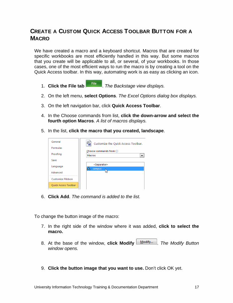
4. In the Choose commands from list, click the down-arrow and select the fourth option Macros. A list of macros displays.

5. In the list, click the macro that you created, landscape.

6. Click Add. The command is added to the list.

To change the button image of the macro:

7. In the right side of the window where it was added, click to select the macro.

8. At the base of the window, click Modify . The Modify Button window opens.

9. Click the button image that you want to use. Don’t click OK yet.


At the base of the window, in the Display name field, is the tooltip that is displayed when you rest the mouse pointer on the button. Alternately, if you wish to change the name of the macro from campus, type the name that you want to use.

10. Click OK. The Modify Button window closes.

11. Click OK. The macro button is added to the Quick Access Toolbar.

To test the new macro tool:

12. On the Quick Access Toolbar, click the campus macro button. The filtered data is placed on a new sheet.

If you make a mistake while recording your macro, or no longer need your macro, you can delete it from within the Macro dialog box. To delete a macro:

1. On the Developer tab, in the Code group, click Macros. The Macro window opens.

2. Select the macro.

3. Click Delete. The prompt, “Do you want to delete…” appears.

4. Click Yes. The macro is removed.

To remove the custom Quick Access button (tool):

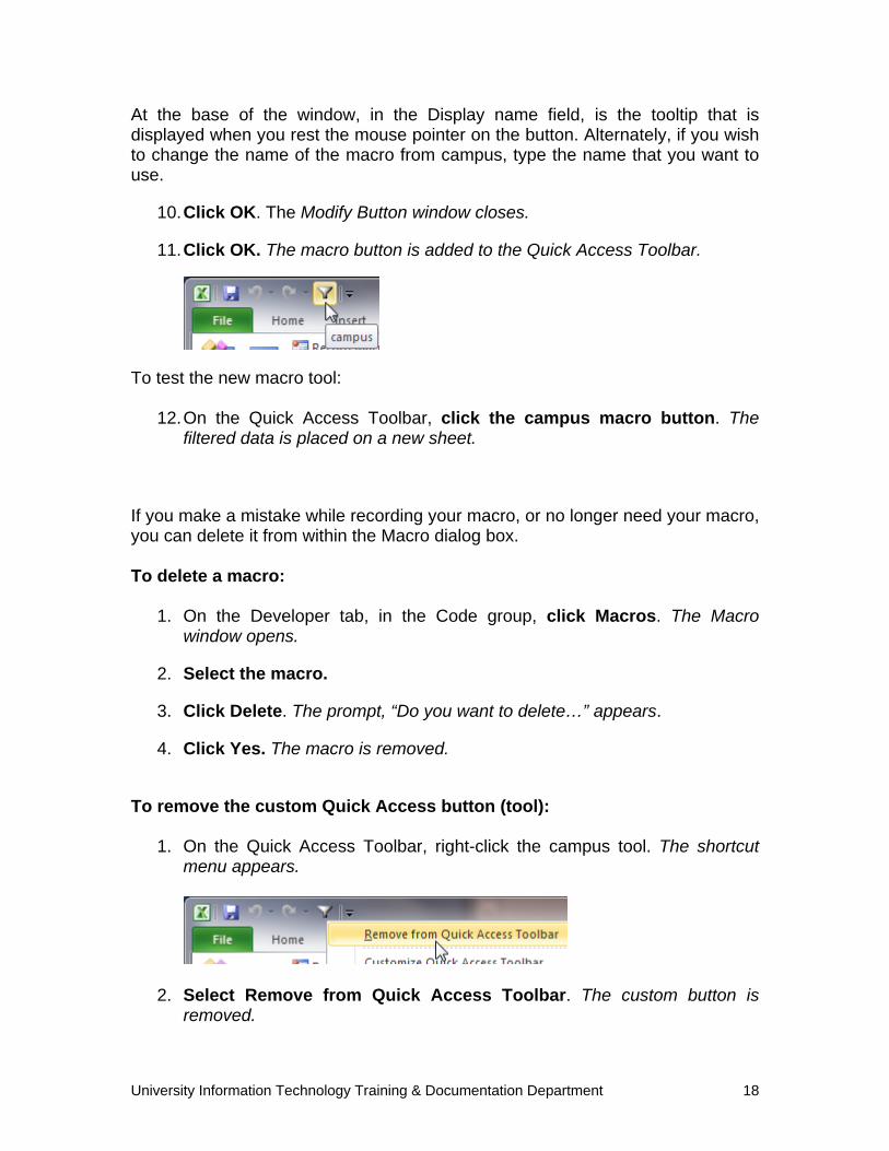
1. On the Quick Access Toolbar, right-click the campus tool. The shortcut menu appears.

2. Select Remove from Quick Access Toolbar. The custom button is removed.


SORTING ROWS OF DATA There are times when you may have a large spreadsheet and you need to manipulate the arrangement of your data to make it more user-friendly. It may be easier to find information when you arrange your data in a logical manner much like a phone book alphabetizes its entries. You may also discover patterns and trends as you sort your data. There may be data that you wish to emphasize because it is more important than other data. Sorting is one method of changing the view of your data to meet different needs. Sort data from smallest to largest and vice versa Excel provides tools on both the Home and Data tabs that will allow you to sort lists alphabetically, numerically, or by date. To sort data from smallest to largest or vice versa:

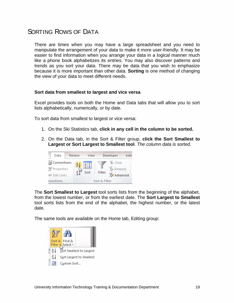
1. On the Ski Statistics tab, click in any cell in the column to be sorted.

2. On the Data tab, in the Sort & Filter group, click the Sort Smallest to Largest or Sort Largest to Smallest tool. The column data is sorted.

The Sort Smallest to Largest tool sorts lists from the beginning of the alphabet, from the lowest number, or from the earliest date. The Sort Largest to Smallest tool sorts lists from the end of the alphabet, the highest number, or the latest date. The same tools are available on the Home tab, Editing group:


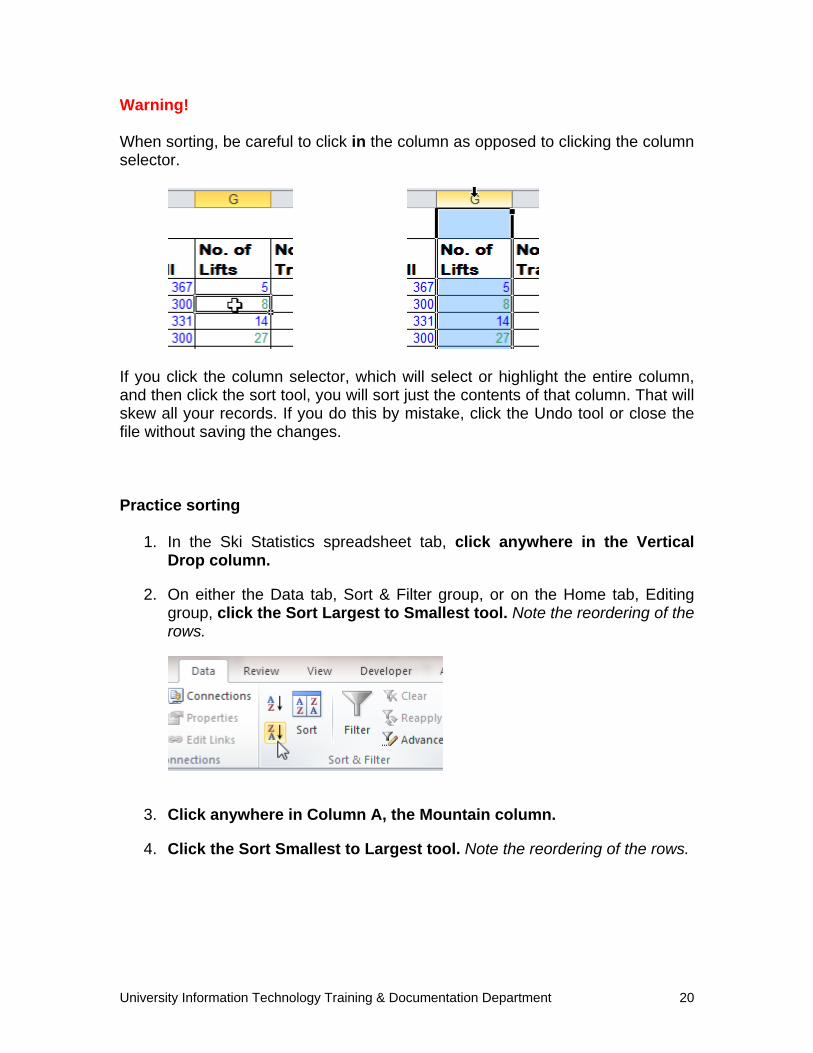
Warning! When sorting, be careful to click in the column as opposed to clicking the column selector.

If you click the column selector, which will select or highlight the entire column, and then click the sort tool, you will sort just the contents of that column. That will skew all your records. If you do this by mistake, click the Undo tool or close the file without saving the changes. Practice sorting

1. In the Ski Statistics spreadsheet tab, click anywhere in the Vertical Drop column.

2. On either the Data tab, Sort & Filter group, or on the Home tab, Editing group, click the Sort Largest to Smallest tool. Note the reordering of the rows.

3. Click anywhere in Column A, the Mountain column.

4. Click the Sort Smallest to Largest tool. Note the reordering of the rows.


SORTING BY MULTIPLE CRITERIA You can take sorting a step further by sorting your rows by more than one column. You choose the order of columns by which you want to sort. The most important column should be the first on your list. Practice sorting by multiple criteria In this example we will sort by two criteria. First we will sort by annual snowfall and then by skiable area.

1. Click anywhere in the table of data.

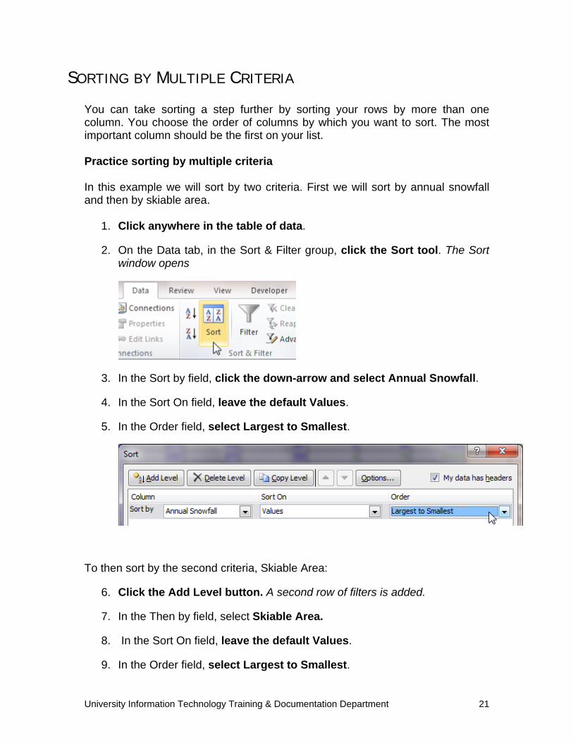
2. On the Data tab, in the Sort & Filter group, click the Sort tool. The Sort window opens

3. In the Sort by field, click the down-arrow and select Annual Snowfall.

4. In the Sort On field, leave the default Values.

5. In the Order field, select Largest to Smallest.

To then sort by the second criteria, Skiable Area:

6. Click the Add Level button. A second row of filters is added.

7. In the Then by field, select Skiable Area.

8. In the Sort On field, leave the default Values.

9. In the Order field, select Largest to Smallest.


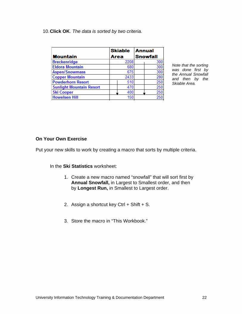
10. Click OK. The data is sorted by two criteria.

On Your Own Exercise Put your new skills to work by creating a macro that sorts by multiple criteria.

In the Ski Statistics worksheet:

1. Create a new macro named “snowfall” that will sort first by Annual Snowfall, in Largest to Smallest order, and then by Longest Run, in Smallest to Largest order.

2. Assign a shortcut key Ctrl + Shift + S. 3. Store the macro in “This Workbook.”

Note that the sorting was done first by the Annual Snowfall and then by the Skiable Area.


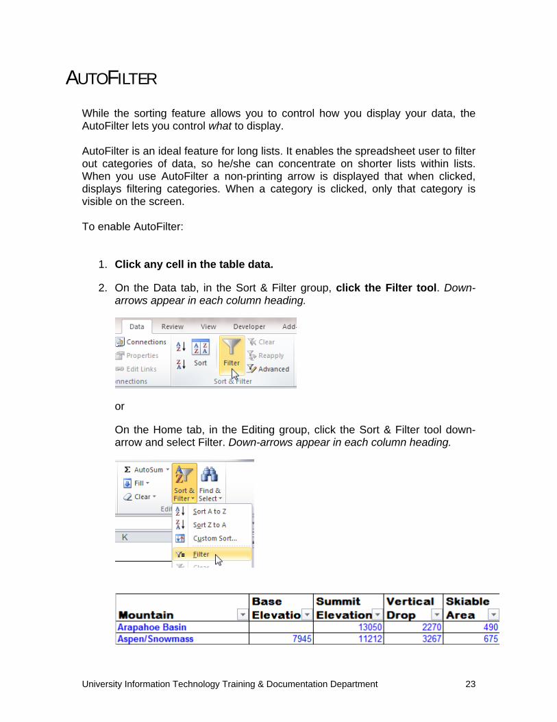
AUTOFILTER While the sorting feature allows you to control how you display your data, the AutoFilter lets you control what to display. AutoFilter is an ideal feature for long lists. It enables the spreadsheet user to filter out categories of data, so he/she can concentrate on shorter lists within lists. When you use AutoFilter a non-printing arrow is displayed that when clicked, displays filtering categories. When a category is clicked, only that category is visible on the screen. To enable AutoFilter:

1. Click any cell in the table data.

2. On the Data tab, in the Sort & Filter group, click the Filter tool. Down-arrows appear in each column heading.

or

On the Home tab, in the Editing group, click the Sort & Filter tool down-arrow and select Filter. Down-arrows appear in each column heading.


Within the AutoFilter feature is the capacity to customize the filtering of a list, column by column. When printing, the down-arrows do not print.

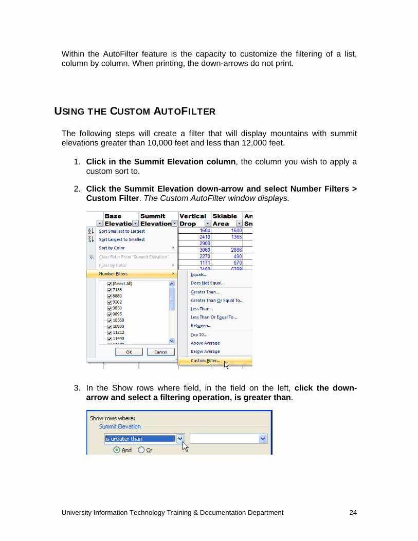
USING THE CUSTOM AUTOFILTER The following steps will create a filter that will display mountains with summit elevations greater than 10,000 feet and less than 12,000 feet.

1. Click in the Summit Elevation column, the column you wish to apply a custom sort to.

2. Click the Summit Elevation down-arrow and select Number Filters > Custom Filter. The Custom AutoFilter window displays.

3. In the Show rows where field, in the field on the left, click the down-

arrow and select a filtering operation, is greater than.


4. Enter a value in the adjacent field on the right, 10000.

To include another set of criteria in the filter, click And or Or, and then use the bottom row of boxes.

5. Click the And option.

6. In the field on the left, click the down-arrow and select a filtering

operation, is less than.

7. In the field to the right, enter 12000.

8. Click OK. The Custom AutoFilter window closes, your filtered results display, and the filter down-arrow icon reflects a funnel icon.

Note that at the base of the window, the left corner of the Status bar also reflects the data set from the filtering operation.

The list has been filtered to show 8 mountains with elevations between 10,000 and 12,000 feet.


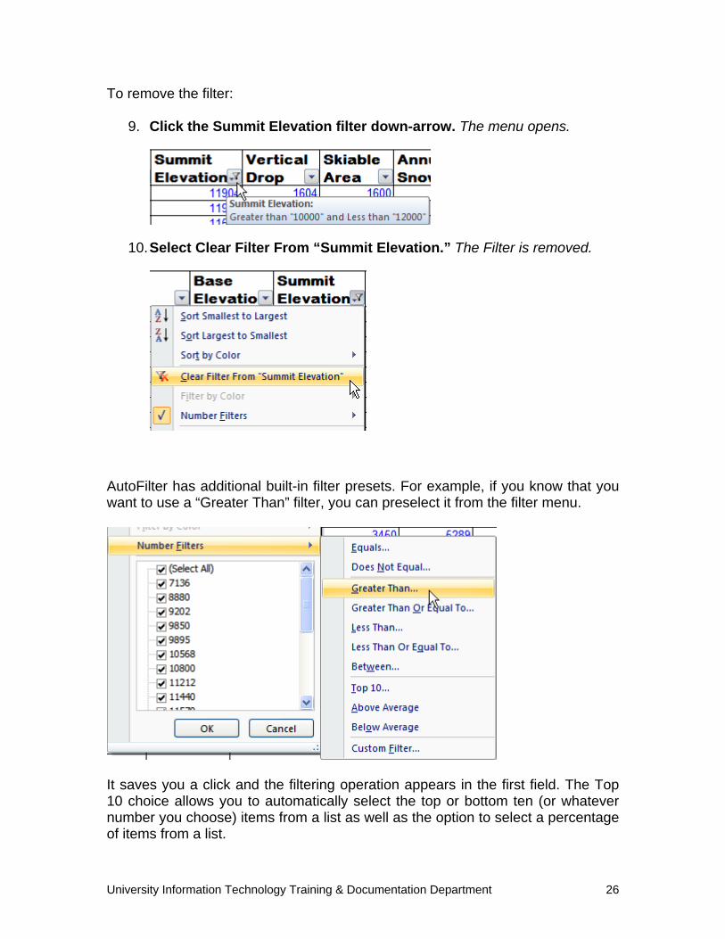
To remove the filter:

9. Click the Summit Elevation filter down-arrow. The menu opens.

10. Select Clear Filter From “Summit Elevation.” The Filter is removed.

AutoFilter has additional built-in filter presets. For example, if you know that you want to use a “Greater Than” filter, you can preselect it from the filter menu.

It saves you a click and the filtering operation appears in the first field. The Top 10 choice allows you to automatically select the top or bottom ten (or whatever number you choose) items from a list as well as the option to select a percentage of items from a list.


To turn off the AutoFilter feature:

1. On the Data tab, in the Sort & Filter group, click the Filter tool. The filter down-arrows are removed from each column heading.

REFERENCING CELLS IN FORMULAS Most of the formulas you create will include at least one reference to a cell. Referencing a cell instead of using fixed values gives you more flexibility when creating formulas. For example, you can change the value of the cell without having to change the actual formula. The formula result automatically reflects the new value. In order to understand how to use references you must first understand the differences between relative and absolute references.

RELATIVE AND ABSOLUTE REFERENCES Relative reference When you copy a formula from one cell to another by using either the copy and paste or the AutoFill feature, the formula remains constant but the cell references change. The references change by the offset from the original row and column. Excel refers to this as relative cell referencing. For example, a formula contains the instructions to add the values of two adjacent cells in a row and multiply that sum by the value of the third cell in that row.

=(A1+B1)*C1

If you copy that formula to a new location, those instructions are copied, not the actual contents of the cell.

=(B4+C4)*D4

If you move a formula, the cell references remain the same and refer to the original cells.

=(A1+B1)*C1


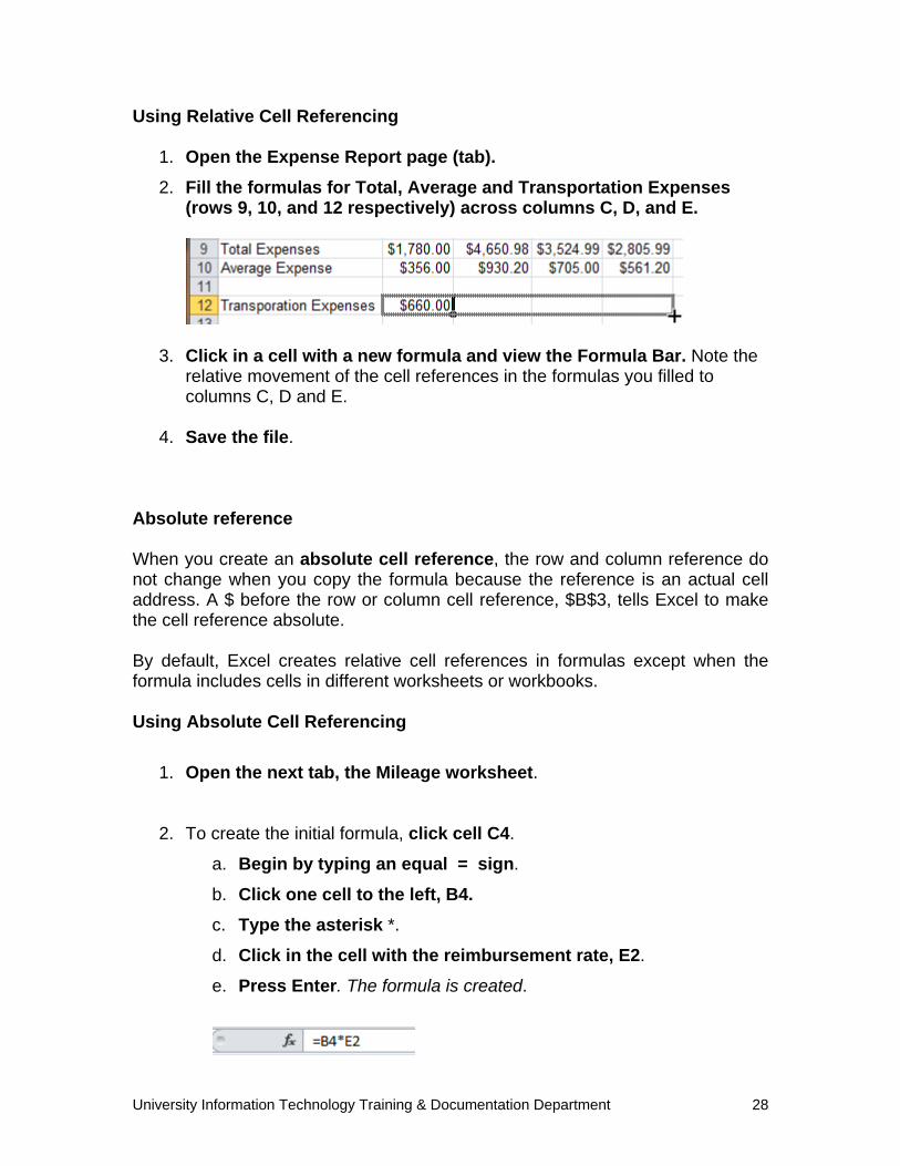
Using Relative Cell Referencing

1. Open the Expense Report page (tab).

2. Fill the formulas for Total, Average and Transportation Expenses (rows 9, 10, and 12 respectively) across columns C, D, and E.

3. Click in a cell with a new formula and view the Formula Bar. Note the relative movement of the cell references in the formulas you filled to columns C, D and E.

4. Save the file.

Absolute reference When you create an absolute cell reference, the row and column reference do not change when you copy the formula because the reference is an actual cell address. A $ before the row or column cell reference, $B$3, tells Excel to make the cell reference absolute. By default, Excel creates relative cell references in formulas except when the formula includes cells in different worksheets or workbooks. Using Absolute Cell Referencing

1. Open the next tab, the Mileage worksheet.

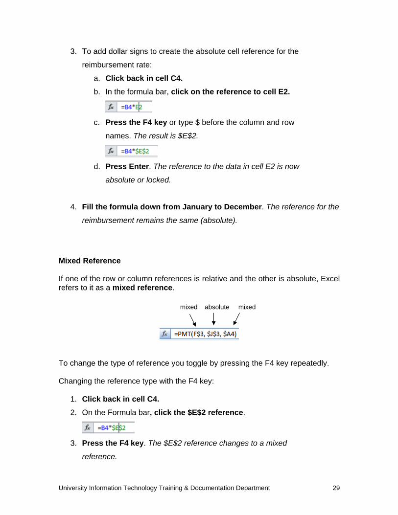
2. To create the initial formula, click cell C4.

a. Begin by typing an equal = sign.

b. Click one cell to the left, B4.

c. Type the asterisk *.

d. Click in the cell with the reimbursement rate, E2.

e. Press Enter. The formula is created.


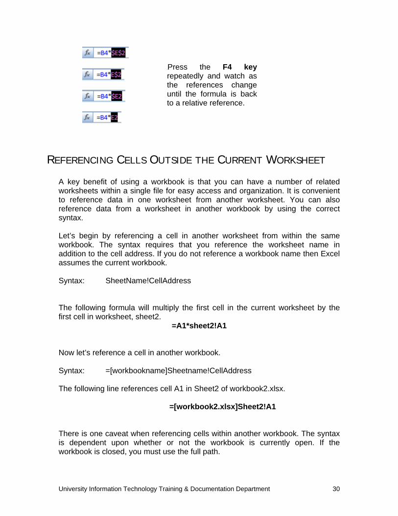
3. To add dollar signs to create the absolute cell reference for the

reimbursement rate:

a. Click back in cell C4.

b. In the formula bar, click on the reference to cell E2.

c. Press the F4 key or type $ before the column and row

names. The result is $E$2.

d. Press Enter. The reference to the data in cell E2 is now

absolute or locked.

4. Fill the formula down from January to December. The reference for the

reimbursement remains the same (absolute).

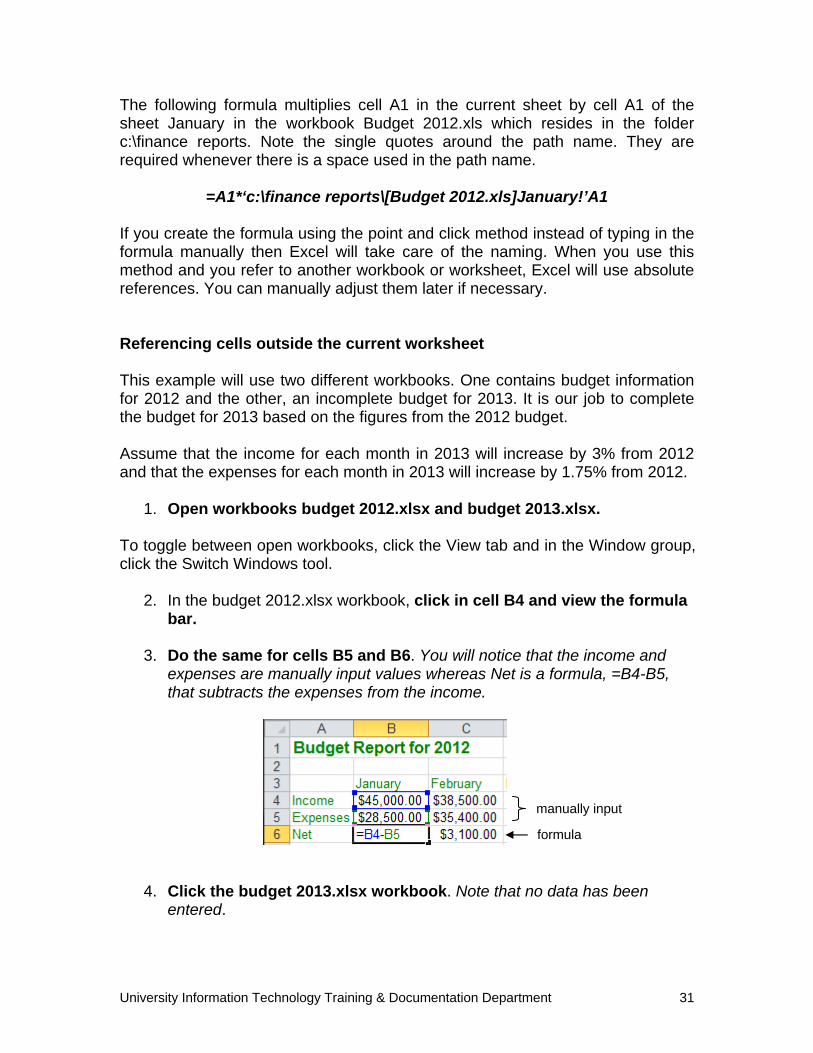
Mixed Reference If one of the row or column references is relative and the other is absolute, Excel refers to it as a mixed reference.

To change the type of reference you toggle by pressing the F4 key repeatedly. Changing the reference type with the F4 key:

1. Click back in cell C4.

2. On the Formula bar, click the $E$2 reference.

3. Press the F4 key. The $E$2 reference changes to a mixed

reference.

mixed absolute mixed


REFERENCING CELLS OUTSIDE THE CURRENT WORKSHEET A key benefit of using a workbook is that you can have a number of related worksheets within a single file for easy access and organization. It is convenient to reference data in one worksheet from another worksheet. You can also reference data from a worksheet in another workbook by using the correct syntax. Let’s begin by referencing a cell in another worksheet from within the same workbook. The syntax requires that you reference the worksheet name in addition to the cell address. If you do not reference a workbook name then Excel assumes the current workbook. Syntax: SheetName!CellAddress The following formula will multiply the first cell in the current worksheet by the first cell in worksheet, sheet2.

=A1*sheet2!A1 Now let’s reference a cell in another workbook. Syntax: =[workbookname]Sheetname!CellAddress The following line references cell A1 in Sheet2 of workbook2.xlsx.

=[workbook2.xlsx]Sheet2!A1 There is one caveat when referencing cells within another workbook. The syntax is dependent upon whether or not the workbook is currently open. If the workbook is closed, you must use the full path.

Press the F4 key repeatedly and watch as the references change until the formula is back to a relative reference.


The following formula multiplies cell A1 in the current sheet by cell A1 of the sheet January in the workbook Budget 2012.xls which resides in the folder c:\finance reports. Note the single quotes around the path name. They are required whenever there is a space used in the path name.

=A1*‘c:\finance reports\[Budget 2012.xls]January!’A1

If you create the formula using the point and click method instead of typing in the formula manually then Excel will take care of the naming. When you use this method and you refer to another workbook or worksheet, Excel will use absolute references. You can manually adjust them later if necessary. Referencing cells outside the current worksheet This example will use two different workbooks. One contains budget information for 2012 and the other, an incomplete budget for 2013. It is our job to complete the budget for 2013 based on the figures from the 2012 budget. Assume that the income for each month in 2013 will increase by 3% from 2012 and that the expenses for each month in 2013 will increase by 1.75% from 2012.

1. Open workbooks budget 2012.xlsx and budget 2013.xlsx. To toggle between open workbooks, click the View tab and in the Window group, click the Switch Windows tool.

2. In the budget 2012.xlsx workbook, click in cell B4 and view the formula bar.

3. Do the same for cells B5 and B6. You will notice that the income and

expenses are manually input values whereas Net is a formula, =B4-B5, that subtracts the expenses from the income.

4. Click the budget 2013.xlsx workbook. Note that no data has been entered.

manually input

formula


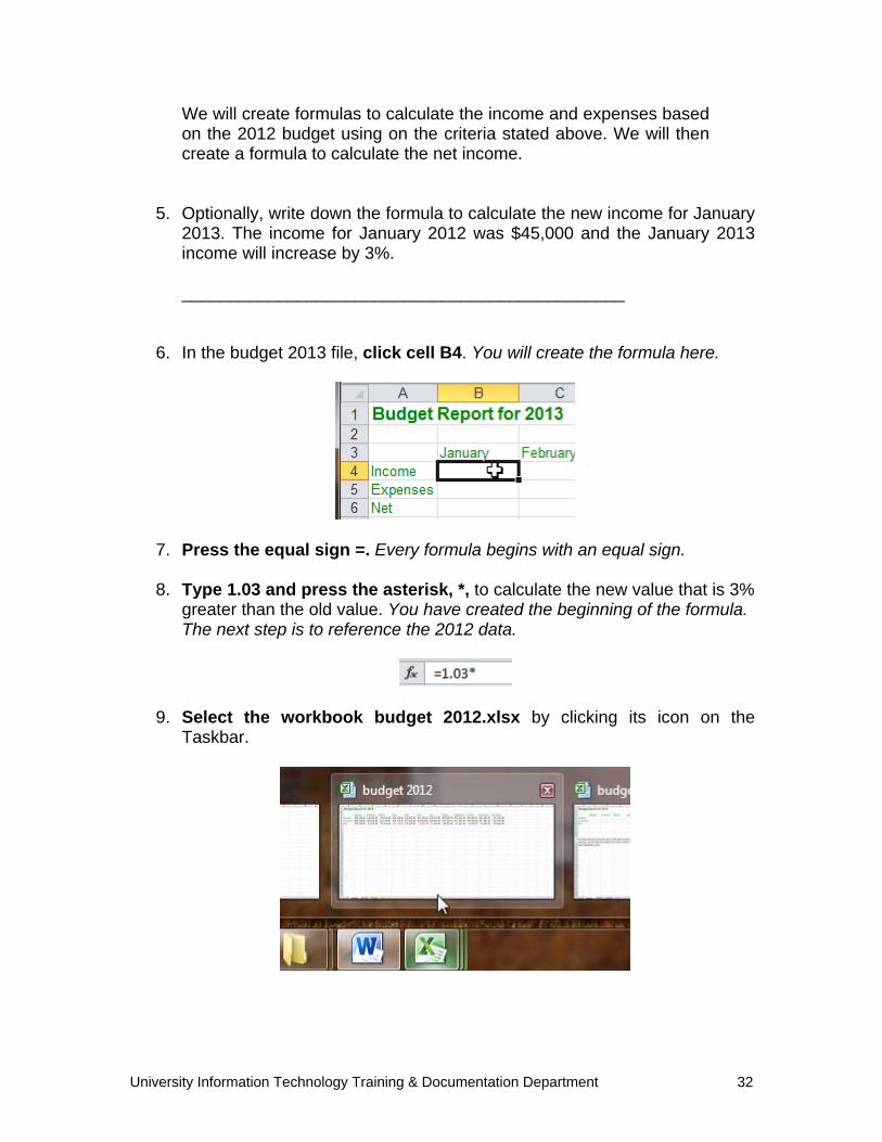
We will create formulas to calculate the income and expenses based on the 2012 budget using on the criteria stated above. We will then create a formula to calculate the net income.

5. Optionally, write down the formula to calculate the new income for January 2013. The income for January 2012 was $45,000 and the January 2013 income will increase by 3%.

______________________________________________

6. In the budget 2013 file, click cell B4. You will create the formula here.

7. Press the equal sign =. Every formula begins with an equal sign.

8. Type 1.03 and press the asterisk, *, to calculate the new value that is 3% greater than the old value. You have created the beginning of the formula. The next step is to reference the 2012 data.

9. Select the workbook budget 2012.xlsx by clicking its icon on the Taskbar.


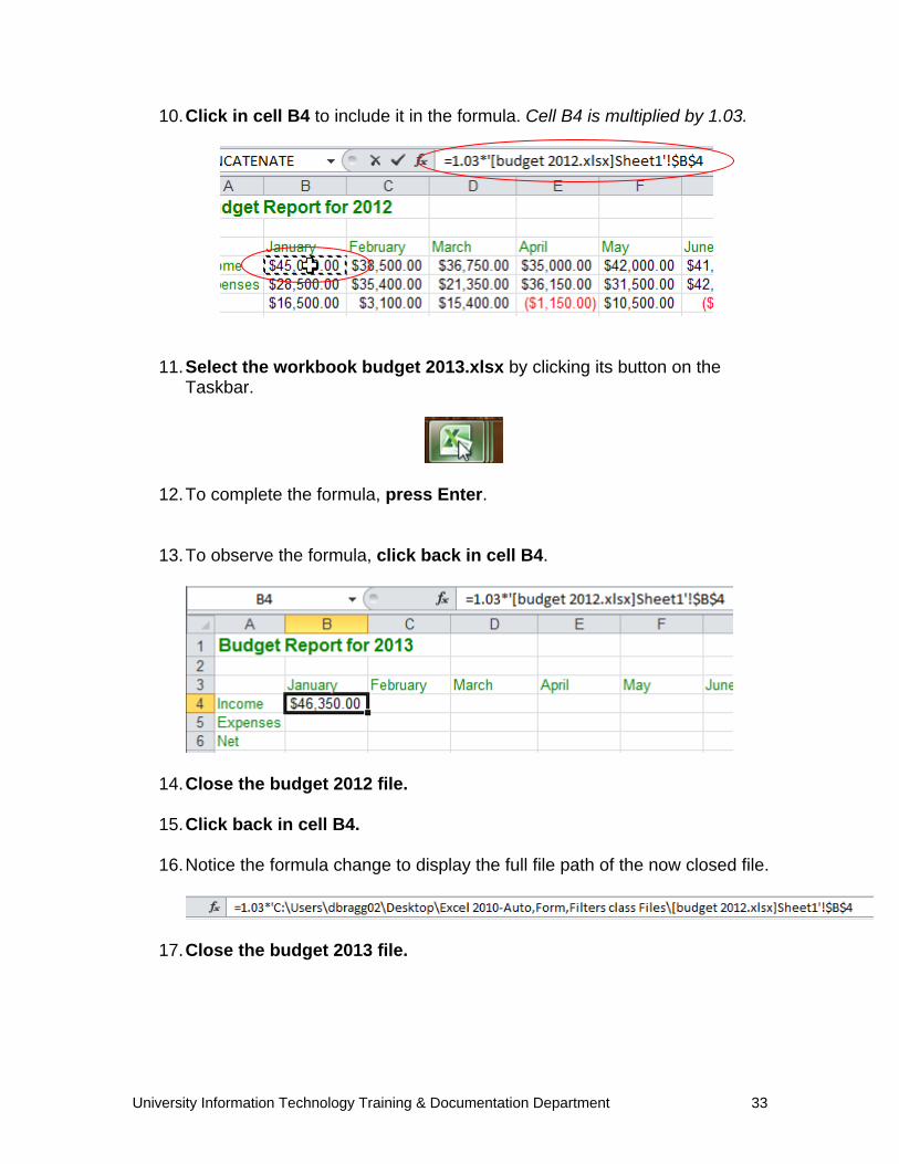
10. Click in cell B4 to include it in the formula. Cell B4 is multiplied by 1.03.

11. Select the workbook budget 2013.xlsx by clicking its button on the Taskbar.

12. To complete the formula, press Enter.

13. To observe the formula, click back in cell B4.

14. Close the budget 2012 file.

15. Click back in cell B4.

16. Notice the formula change to display the full file path of the now closed file.

17. Close the budget 2013 file.


Formula and Functions Formulas and Functions in Excel Use formulas and functions to perform calculations on the data in your worksheets. When you change either the data or the formula, the results are automatically updated. Formulas use arithmetic operators to work with values, text, worksheet functions, and other formulas to calculate a value on a cell. A function is a predefined formula that performs calculations. Functions can be used to perform simple or complex calculations. Before we begin creating formulas, we should review the rules of precedence for mathematical operators.

Operator Description Precedence in Calculations

Mathematical Operators

() Parenthesis 1 ^ Exponentiation 2 * Multiplication 3 / Division 3 + Addition 4 - Subtraction 4

Text Operator

& Concatenation 5

Logical Operators = Equal to 6 < Less than 6 > Greater than 6

<= Less than or equal to 6 >= Greater than or equal to 6 <> Not equal to 6


Review A formula starts with an equal sign (=). This enables excel to distinguish formulas from text. The maximum size of a formula is 1024 characters. After you enter a formula in a cell, the cell displays the results of the formula. The formula itself appears in the formula bar. Create a formula in Excel

1. Click the cell where you want the answer to be displayed.

2. Type “=”, an equal sign.

3. Click the cell with the first number you want to use.

4. Type an operator (e.g. / , * , -, or +).

5. Click the cell with the next number you want to use in your calculation.

6. Repeat steps 4 and 5 as necessary.

7. Press Enter.

AUTOSUM AutoSum is a built-in Excel function that provides a quick method to add a range of numbers from a column or row.

1. Return to the Ski Statistics sheet.

2. Click the cell directly beneath the column that you wish to sum or to the right of the row that you wish to sum.


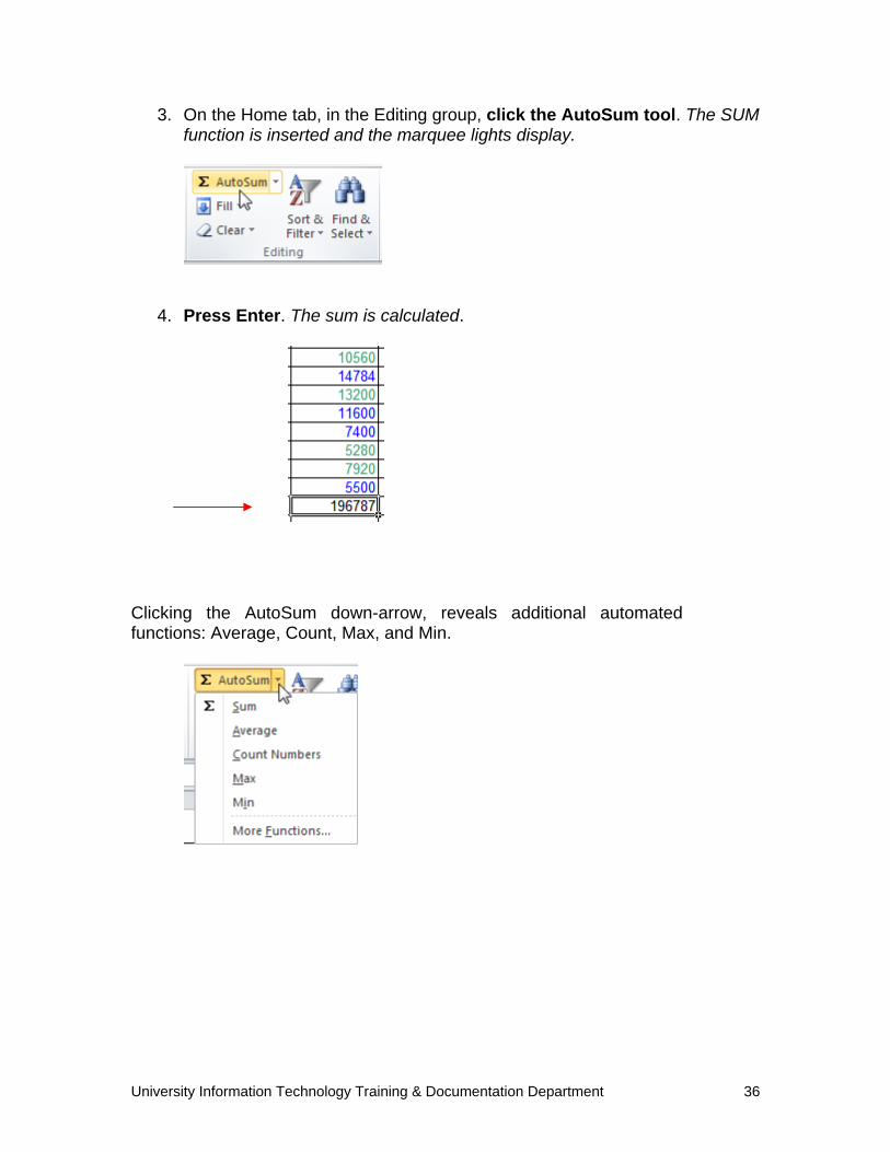
3. On the Home tab, in the Editing group, click the AutoSum tool. The SUM function is inserted and the marquee lights display.

4. Press Enter. The sum is calculated.

Clicking the AutoSum down-arrow, reveals additional automated functions: Average, Count, Max, and Min.


Using AutoCalculate There will be times that you may want to quickly sum a column or row, or a portion of a column or row, but you do not need to record the information on the spreadsheet. The AutoCalculate feature in Excel is ideal for obtaining quick results for several built-in functions. The following functions are included in the Auto Calculate feature:

Average

Count (Counts the number of cells that contain numbers and also

numbers within the list of arguments)

Count Nums (counts the number of cells that contain numbers)

Max (maximum value of a given range)

Min (minimum value of a given range).

Sum

To use AutoCalculate:

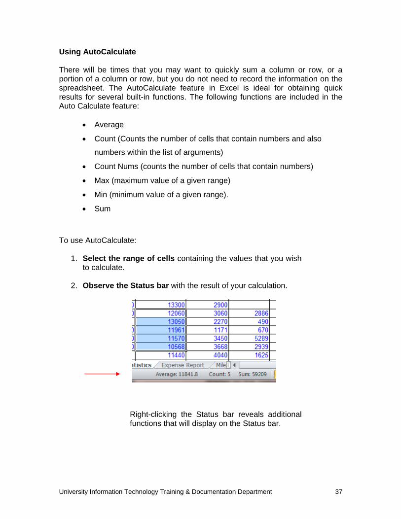
1. Select the range of cells containing the values that you wish to calculate.

2. Observe the Status bar with the result of your calculation.

Right-clicking the Status bar reveals additional functions that will display on the Status bar.


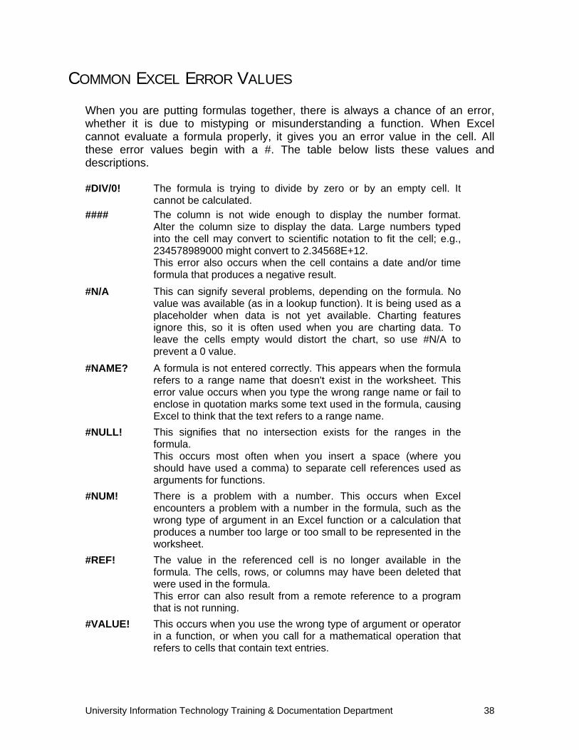
COMMON EXCEL ERROR VALUES When you are putting formulas together, there is always a chance of an error, whether it is due to mistyping or misunderstanding a function. When Excel cannot evaluate a formula properly, it gives you an error value in the cell. All these error values begin with a #. The table below lists these values and descriptions. #DIV/0! The formula is trying to divide by zero or by an empty cell. It

cannot be calculated. #### The column is not wide enough to display the number format.

Alter the column size to display the data. Large numbers typed into the cell may convert to scientific notation to fit the cell; e.g., 234578989000 might convert to 2.34568E+12. This error also occurs when the cell contains a date and/or time formula that produces a negative result.

#N/A This can signify several problems, depending on the formula. No value was available (as in a lookup function). It is being used as a placeholder when data is not yet available. Charting features ignore this, so it is often used when you are charting data. To leave the cells empty would distort the chart, so use #N/A to prevent a 0 value.

#NAME? A formula is not entered correctly. This appears when the formula refers to a range name that doesn't exist in the worksheet. This error value occurs when you type the wrong range name or fail to enclose in quotation marks some text used in the formula, causing Excel to think that the text refers to a range name.

#NULL! This signifies that no intersection exists for the ranges in the formula. This occurs most often when you insert a space (where you should have used a comma) to separate cell references used as arguments for functions.

#NUM! There is a problem with a number. This occurs when Excel encounters a problem with a number in the formula, such as the wrong type of argument in an Excel function or a calculation that produces a number too large or too small to be represented in the worksheet.

#REF! The value in the referenced cell is no longer available in the formula. The cells, rows, or columns may have been deleted that were used in the formula. This error can also result from a remote reference to a program that is not running.

#VALUE! This occurs when you use the wrong type of argument or operator in a function, or when you call for a mathematical operation that refers to cells that contain text entries.


THE INSERT FUNCTION DIALOG BOX When you create a formula that contains a function, the Insert Function dialog box helps you enter worksheet functions. As you enter a function into the formula, the Insert Function dialog box displays the name of the function, each of its arguments, a description of the function and each argument, the current result of the function, and the current result of the entire formula. Functions are predefined calculations that perform a specialized task you use in formulas. You can also use conditional statements and have one calculation performed if a condition exists and another performed if it doesn’t exist. All functions have one thing in common; they are all followed by parentheses, which often include arguments. To refer to an entire row or column as an argument, the syntax is =Average(B:B).

USING FUNCTIONS We will find the average summit elevation of the mountains listed in the Ski Statistics sheet. To use the Insert Function feature:

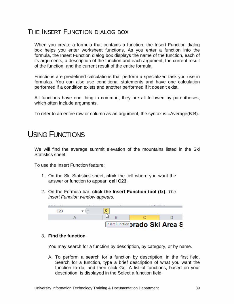
1. On the Ski Statistics sheet, click the cell where you want the answer or function to appear, cell C23.

2. On the Formula bar, click the Insert Function tool (fx). The

Insert Function window appears.

3. Find the function.

You may search for a function by description, by category, or by name.

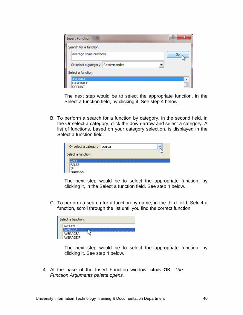
A. To perform a search for a function by description, in the first field, Search for a function, type a brief description of what you want the function to do, and then click Go. A list of functions, based on your description, is displayed in the Select a function field.


The next step would be to select the appropriate function, in the Select a function field, by clicking it. See step 4 below.

B. To perform a search for a function by category, in the second field, in the Or select a category, click the down-arrow and select a category. A list of functions, based on your category selection, is displayed in the Select a function field.

The next step would be to select the appropriate function, by clicking it, in the Select a function field. See step 4 below.

C. To perform a search for a function by name, in the third field, Select a function, scroll through the list until you find the correct function.

The next step would be to select the appropriate function, by clicking it. See step 4 below.

4. At the base of the Insert Function window, click OK. The Function Arguments palette opens.


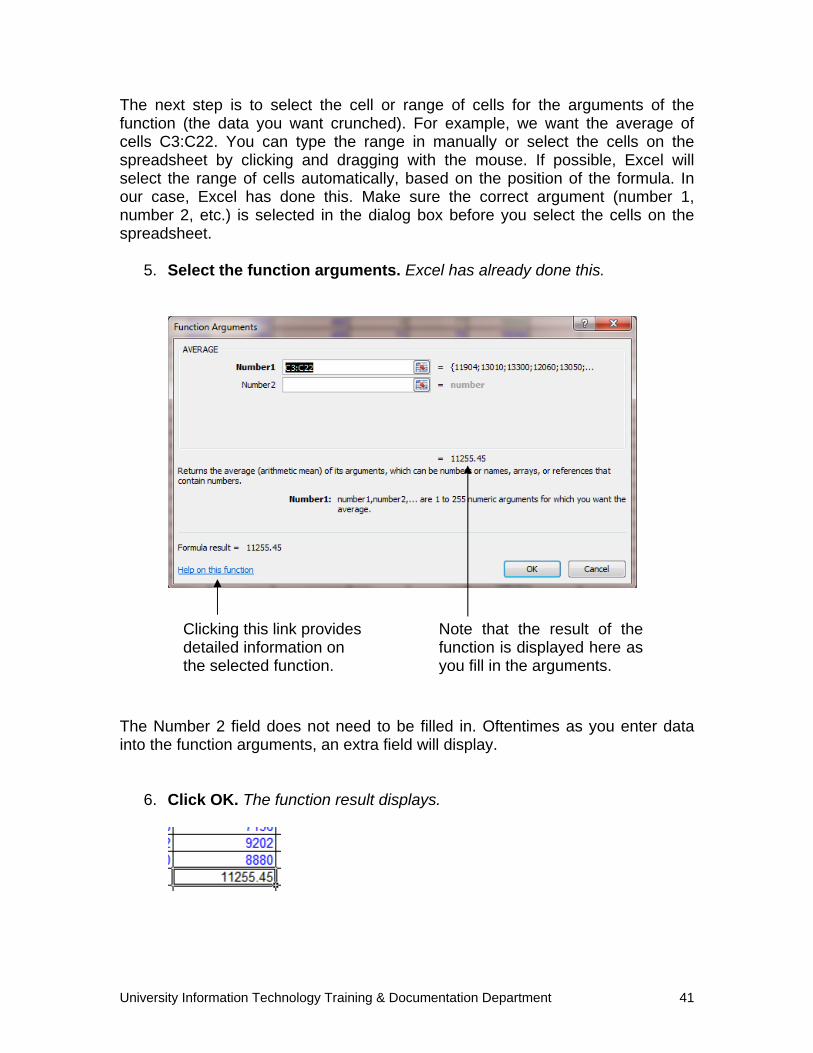
The next step is to select the cell or range of cells for the arguments of the function (the data you want crunched). For example, we want the average of cells C3:C22. You can type the range in manually or select the cells on the spreadsheet by clicking and dragging with the mouse. If possible, Excel will select the range of cells automatically, based on the position of the formula. In our case, Excel has done this. Make sure the correct argument (number 1, number 2, etc.) is selected in the dialog box before you select the cells on the spreadsheet.

5. Select the function arguments. Excel has already done this.

The Number 2 field does not need to be filled in. Oftentimes as you enter data into the function arguments, an extra field will display.

6. Click OK. The function result displays.

Note that the result of the function is displayed here as you fill in the arguments.

Clicking this link provides detailed information on the selected function.


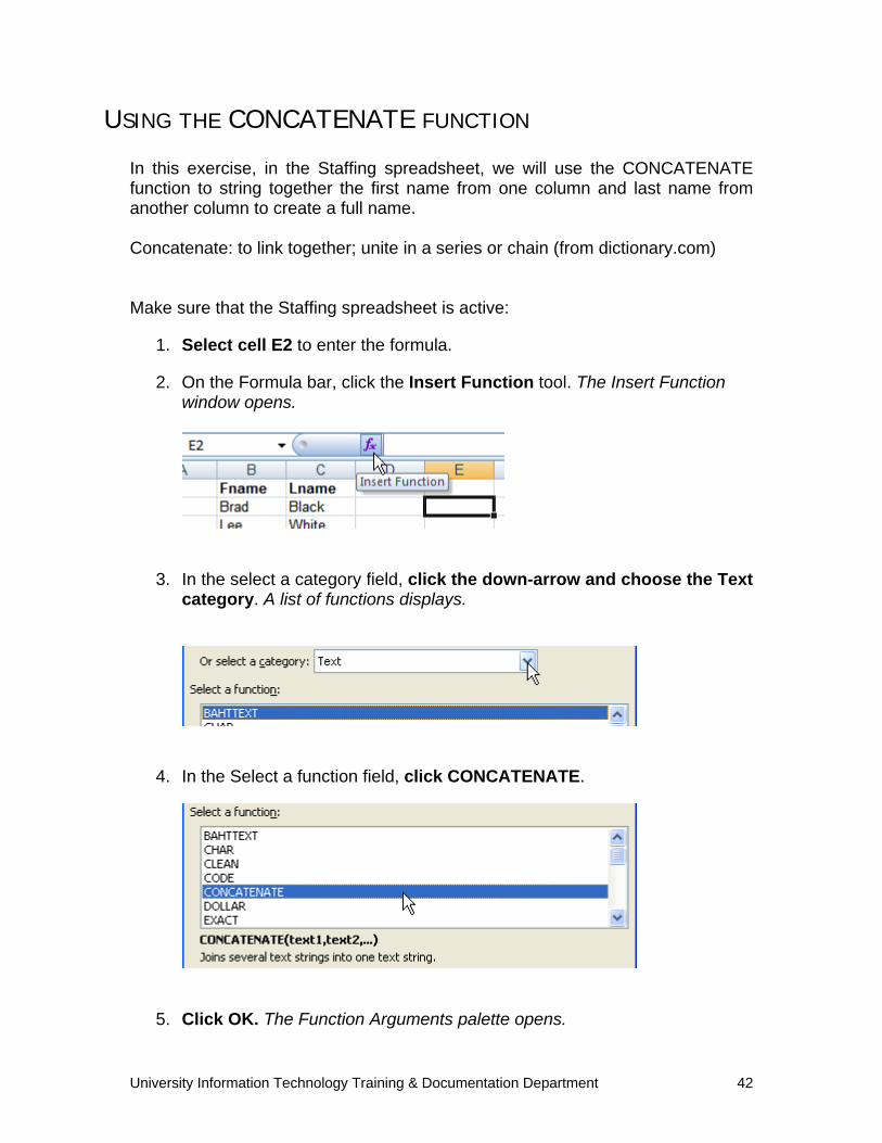
USING THE CONCATENATE FUNCTION In this exercise, in the Staffing spreadsheet, we will use the CONCATENATE function to string together the first name from one column and last name from another column to create a full name. Concatenate: to link together; unite in a series or chain (from dictionary.com) Make sure that the Staffing spreadsheet is active:

1. Select cell E2 to enter the formula.

2. On the Formula bar, click the Insert Function tool. The Insert Function window opens.

3. In the select a category field, click the down-arrow and choose the Text category. A list of functions displays.

4. In the Select a function field, click CONCATENATE.

5. Click OK. The Function Arguments palette opens.


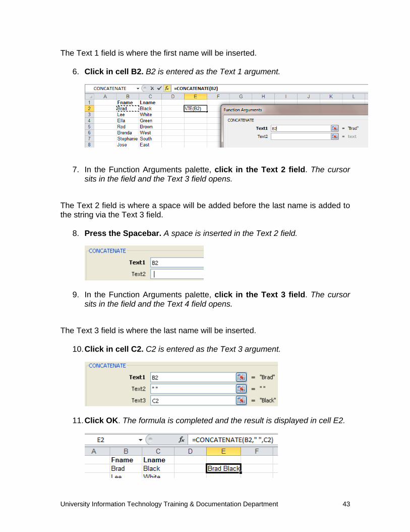
The Text 1 field is where the first name will be inserted.

6. Click in cell B2. B2 is entered as the Text 1 argument.

7. In the Function Arguments palette, click in the Text 2 field. The cursor

sits in the field and the Text 3 field opens.

The Text 2 field is where a space will be added before the last name is added to the string via the Text 3 field.

8. Press the Spacebar. A space is inserted in the Text 2 field.

9. In the Function Arguments palette, click in the Text 3 field. The cursor sits in the field and the Text 4 field opens.

The Text 3 field is where the last name will be inserted.

10. Click in cell C2. C2 is entered as the Text 3 argument.

11. Click OK. The formula is completed and the result is displayed in cell E2.


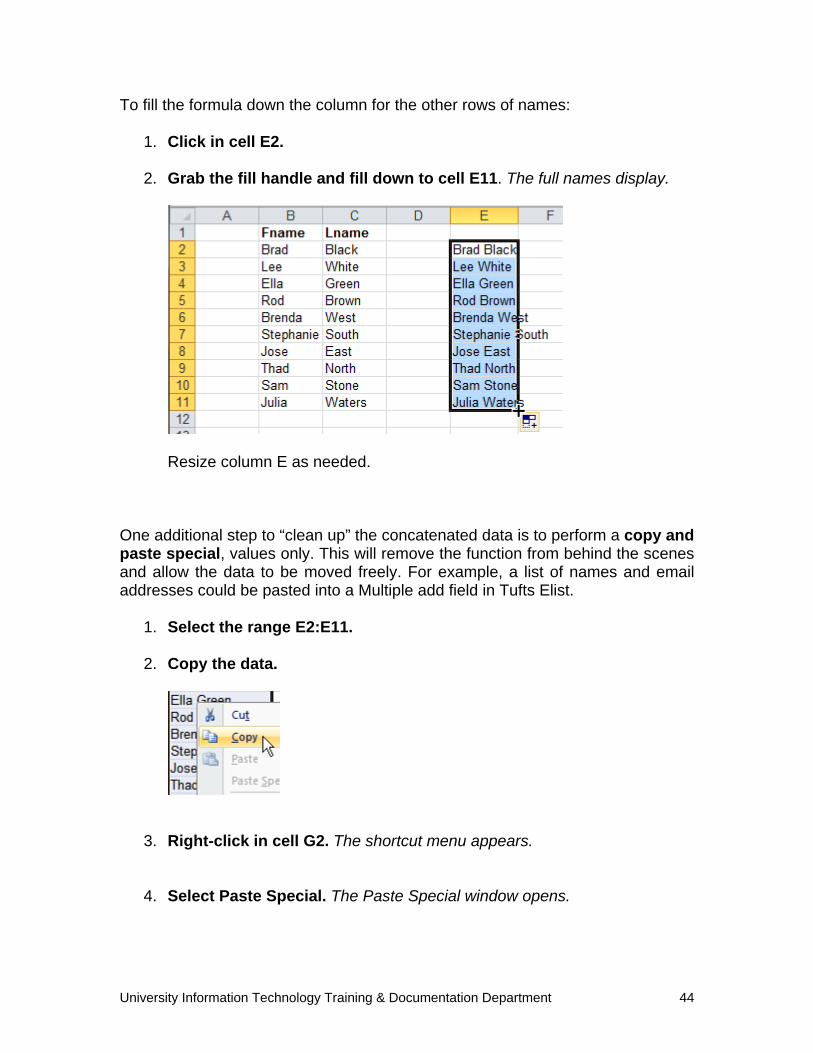
To fill the formula down the column for the other rows of names:

1. Click in cell E2.

2. Grab the fill handle and fill down to cell E11. The full names display.

Resize column E as needed. One additional step to “clean up” the concatenated data is to perform a copy and paste special, values only. This will remove the function from behind the scenes and allow the data to be moved freely. For example, a list of names and email addresses could be pasted into a Multiple add field in Tufts Elist.

1. Select the range E2:E11.

2. Copy the data.

3. Right-click in cell G2. The shortcut menu appears.

4. Select Paste Special. The Paste Special window opens.


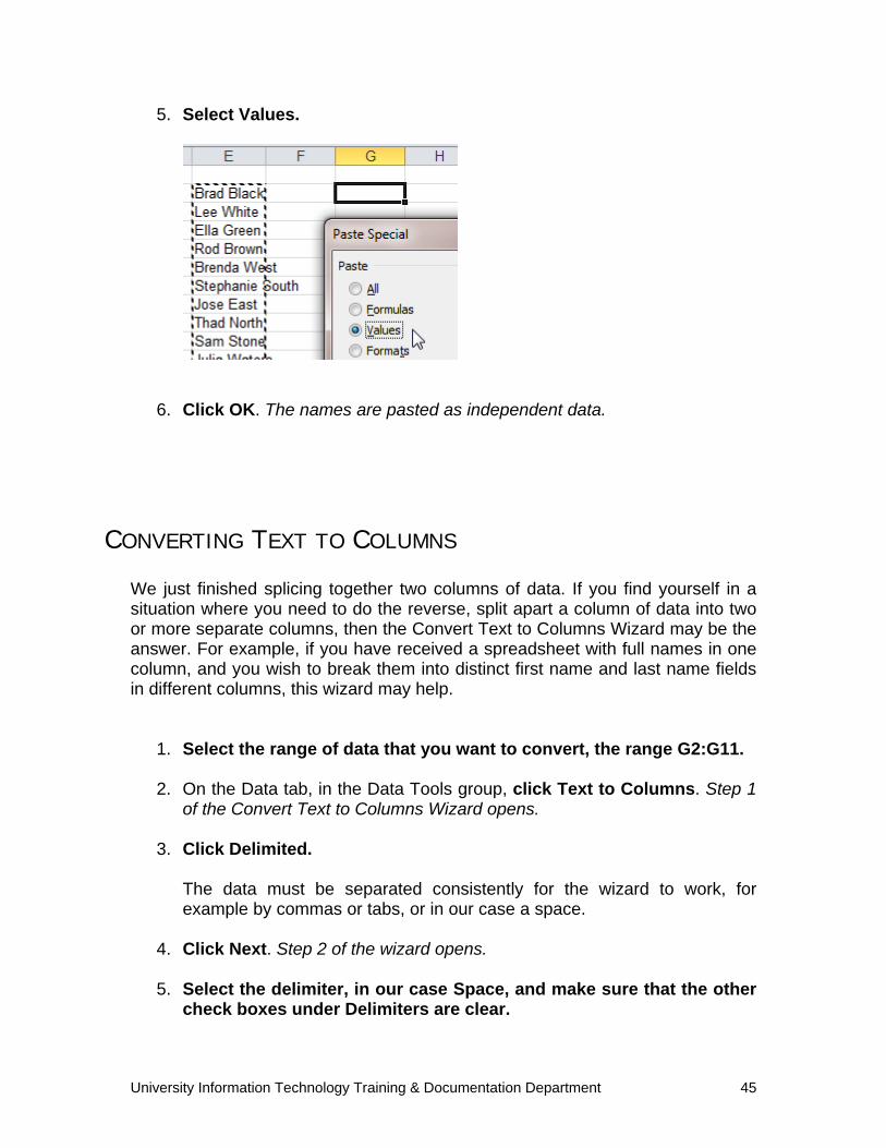
5. Select Values.

6. Click OK. The names are pasted as independent data.

CONVERTING TEXT TO COLUMNS We just finished splicing together two columns of data. If you find yourself in a situation where you need to do the reverse, split apart a column of data into two or more separate columns, then the Convert Text to Columns Wizard may be the answer. For example, if you have received a spreadsheet with full names in one column, and you wish to break them into distinct first name and last name fields in different columns, this wizard may help.

1. Select the range of data that you want to convert, the range G2:G11.

2. On the Data tab, in the Data Tools group, click Text to Columns. Step 1 of the Convert Text to Columns Wizard opens.

3. Click Delimited.

The data must be separated consistently for the wizard to work, for example by commas or tabs, or in our case a space.

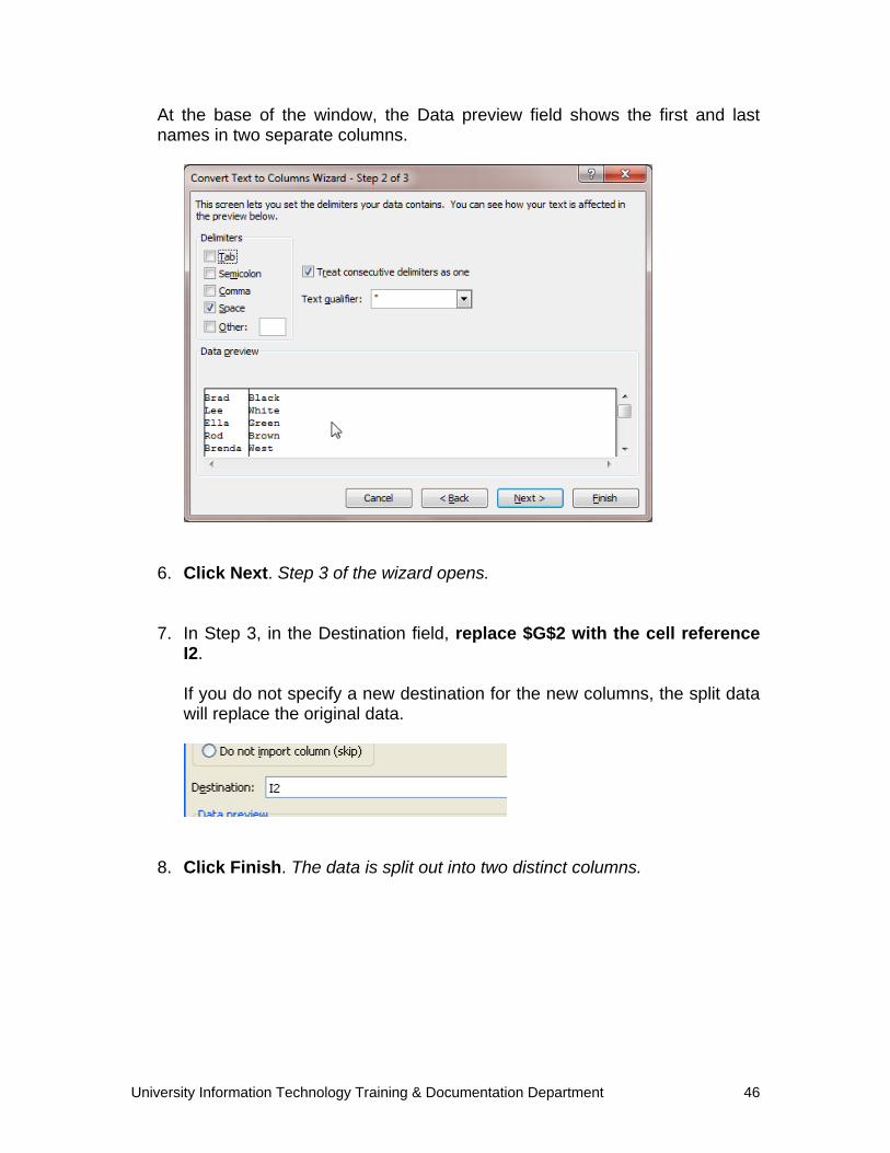
4. Click Next. Step 2 of the wizard opens.

5. Select the delimiter, in our case Space, and make sure that the other

check boxes under Delimiters are clear.


At the base of the window, the Data preview field shows the first and last names in two separate columns.

6. Click Next. Step 3 of the wizard opens.

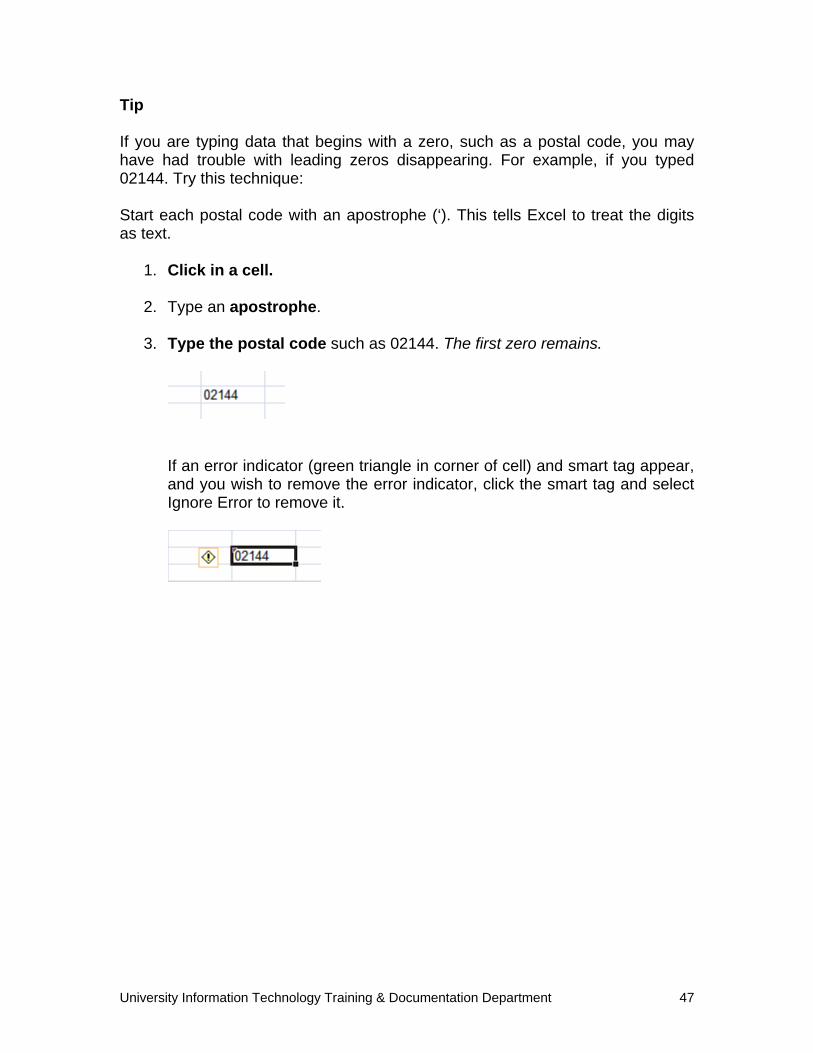
7. In Step 3, in the Destination field, replace $G$2 with the cell reference I2.

If you do not specify a new destination for the new columns, the split data will replace the original data.

8. Click Finish. The data is split out into two distinct columns.


Tip If you are typing data that begins with a zero, such as a postal code, you may have had trouble with leading zeros disappearing. For example, if you typed 02144. Try this technique: Start each postal code with an apostrophe (‘). This tells Excel to treat the digits as text.

1. Click in a cell.

2. Type an apostrophe.

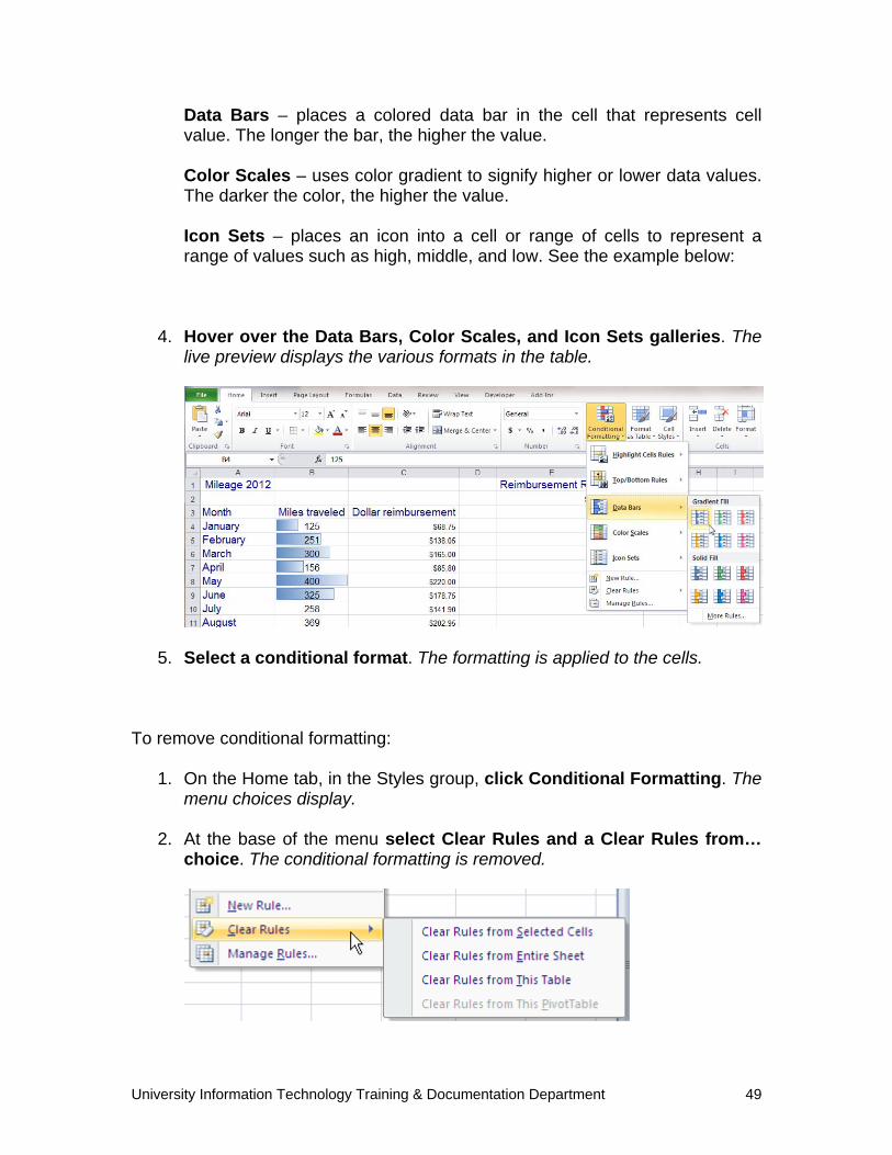
3. Type the postal code such as 02144. The first zero remains.

If an error indicator (green triangle in corner of cell) and smart tag appear, and you wish to remove the error indicator, click the smart tag and select Ignore Error to remove it.


CONDITIONAL FORMATTING The conditional formatting feature in Excel is a method of visually marking cell contents so that certain data can be quickly noted. You set up the rules that mark data. The formatting options include such visual clues as color gradients or icon sets such as colored flags. An example of conditional formatting would be a rule that turns the cell values from black to red of any miles traveled that exceeded the 300 mile threshold.

1. Click the Mileage tab.

2. Select the range of data to display the conditional formatting. In the graphic below, the range B4:B9 has been selected.

3. On the Home tab, in the Styles group, click Conditional Formatting. The conditional formatting menu choices display.

Conditional formats include:

Highlight Cells Rules – marks cell data that is greater, less than, or equal to a value, contains specific text or duplicate values, including dates.

Top/Bottom Rules - marks cell data that falls within high, low, or average values such as Top 10%.


Data Bars – places a colored data bar in the cell that represents cell value. The longer the bar, the higher the value.

Color Scales – uses color gradient to signify higher or lower data values. The darker the color, the higher the value.

Icon Sets – places an icon into a cell or range of cells to represent a range of values such as high, middle, and low. See the example below:

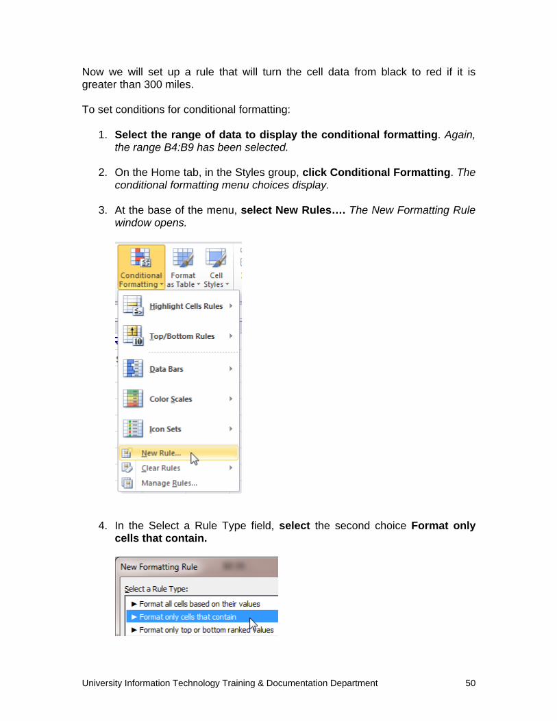
4. Hover over the Data Bars, Color Scales, and Icon Sets galleries. The live preview displays the various formats in the table.

5. Select a conditional format. The formatting is applied to the cells. To remove conditional formatting:

1. On the Home tab, in the Styles group, click Conditional Formatting. The menu choices display.

2. At the base of the menu select Clear Rules and a Clear Rules from…

choice. The conditional formatting is removed.


Now we will set up a rule that will turn the cell data from black to red if it is greater than 300 miles. To set conditions for conditional formatting:

1. Select the range of data to display the conditional formatting. Again, the range B4:B9 has been selected.

2. On the Home tab, in the Styles group, click Conditional Formatting. The

conditional formatting menu choices display.

3. At the base of the menu, select New Rules…. The New Formatting Rule window opens.

4. In the Select a Rule Type field, select the second choice Format only cells that contain.


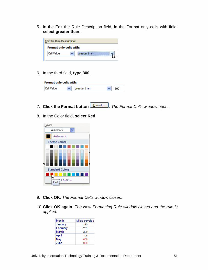
5. In the Edit the Rule Description field, in the Format only cells with field, select greater than.

6. In the third field, type 300.

7. Click the Format button . The Format Cells window open.

8. In the Color field, select Red.

9. Click OK. The Format Cells window closes.

10. Click OK again. The New Formatting Rule window closes and the rule is applied.


To adjust conditional formatting:

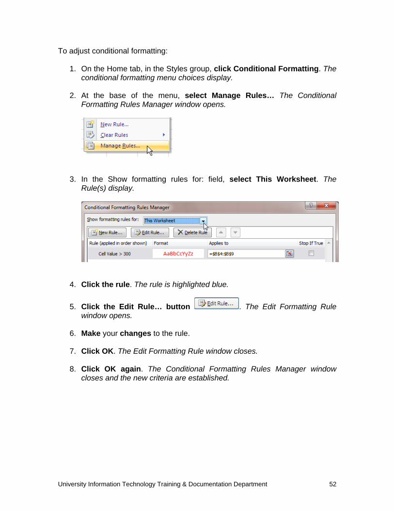
1. On the Home tab, in the Styles group, click Conditional Formatting. The conditional formatting menu choices display.

2. At the base of the menu, select Manage Rules… The Conditional

Formatting Rules Manager window opens.

3. In the Show formatting rules for: field, select This Worksheet. The Rule(s) display.

4. Click the rule. The rule is highlighted blue.

5. Click the Edit Rule… button . The Edit Formatting Rule window opens.

6. Make your changes to the rule.

7. Click OK. The Edit Formatting Rule window closes.

8. Click OK again. The Conditional Formatting Rules Manager window

closes and the new criteria are established.


DATA VALIDATION Data validation is a tool employed to control the data that users enter into a cell or range of cells so that data entered into a workbook is accurate. For example, you can restrict data entry to a certain range of numbers. You can set up data validation to prevent users from entering data that is not valid or you can allow users to enter invalid data but warn them when they try to type it in the cell. You can also write warning messages to clarify data input guidelines and instructions to help users correct their errors. To set up data validation:

1. Click the Expense Report tab.

2. Select the range of cells B3:E7. The expense data is selected.

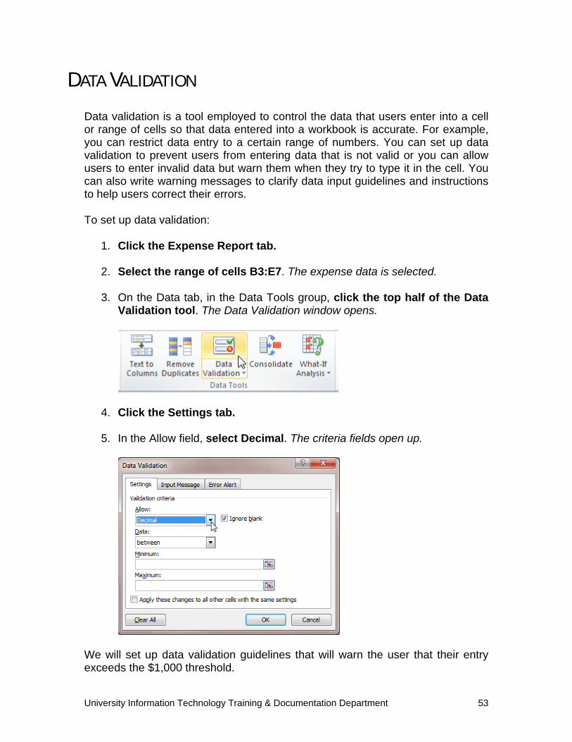
3. On the Data tab, in the Data Tools group, click the top half of the Data Validation tool. The Data Validation window opens.

4. Click the Settings tab.

5. In the Allow field, select Decimal. The criteria fields open up.

We will set up data validation guidelines that will warn the user that their entry exceeds the $1,000 threshold.


6. In the Data field, click the drop-down and select less than. This will set the upper limit.

7. In the Maximum field, type1000. This limits data entry to $999.99.

To set the message (Error Alert) when incorrect data is entered:

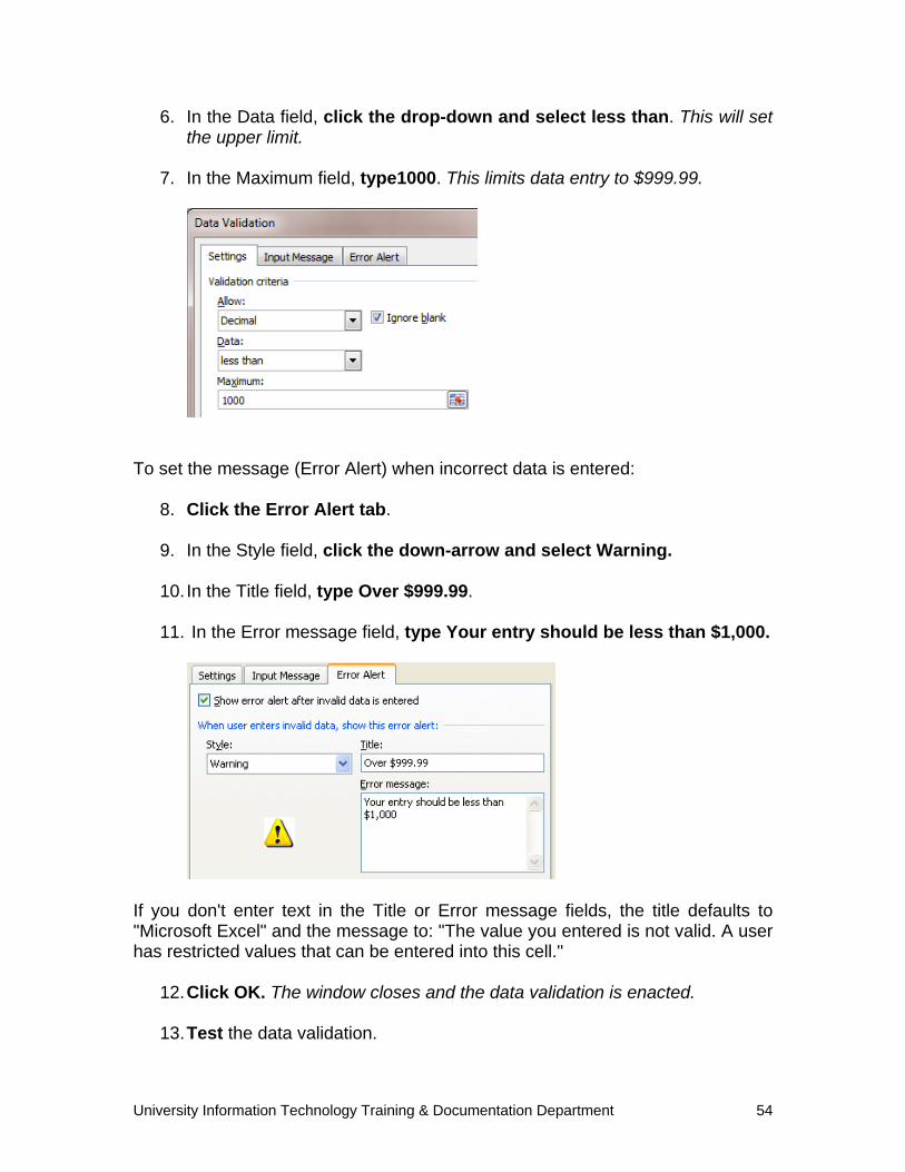
8. Click the Error Alert tab.

9. In the Style field, click the down-arrow and select Warning.

10. In the Title field, type Over $999.99.

11. In the Error message field, type Your entry should be less than $1,000.

If you don't enter text in the Title or Error message fields, the title defaults to "Microsoft Excel" and the message to: "The value you entered is not valid. A user has restricted values that can be entered into this cell."

12. Click OK. The window closes and the data validation is enacted.

13. Test the data validation.


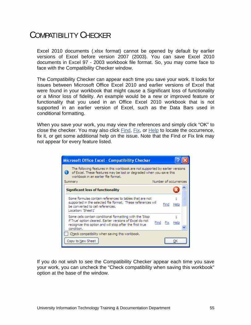
COMPATIBILITY CHECKER Excel 2010 documents (.xlsx format) cannot be opened by default by earlier versions of Excel before version 2007 (2003). You can save Excel 2010 documents in Excel 97 - 2003 workbook file format. So, you may come face to face with the Compatibility Checker window. The Compatibility Checker can appear each time you save your work. It looks for issues between Microsoft Office Excel 2010 and earlier versions of Excel that were found in your workbook that might cause a Significant loss of functionality or a Minor loss of fidelity. An example would be a new or improved feature or functionality that you used in an Office Excel 2010 workbook that is not supported in an earlier version of Excel, such as the Data Bars used in conditional formatting. When you save your work, you may view the references and simply click “OK” to close the checker. You may also click Find, Fix, or Help to locate the occurrence, fix it, or get some additional help on the issue. Note that the Find or Fix link may not appear for every feature listed.

If you do not wish to see the Compatibility Checker appear each time you save your work, you can uncheck the “Check compatibility when saving this workbook” option at the base of the window.


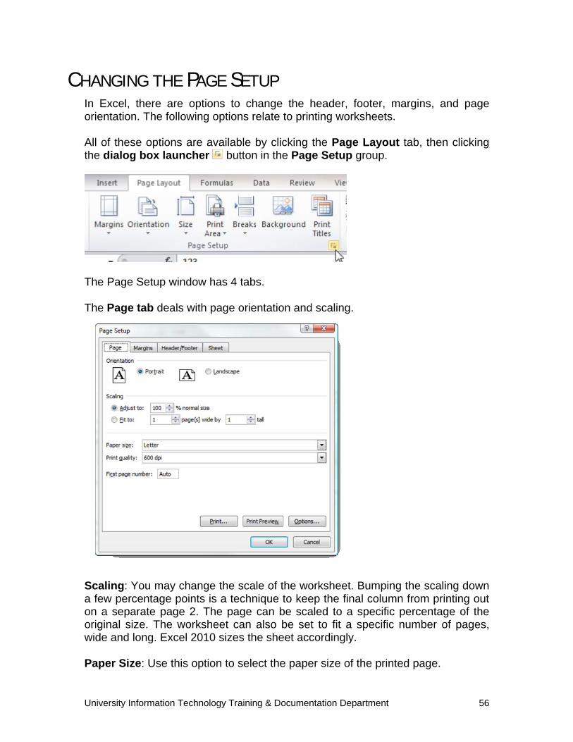
CHANGING THE PAGE SETUP In Excel, there are options to change the header, footer, margins, and page orientation. The following options relate to printing worksheets. All of these options are available by clicking the Page Layout tab, then clicking the dialog box launcher button in the Page Setup group.

The Page Setup window has 4 tabs. The Page tab deals with page orientation and scaling.

Scaling: You may change the scale of the worksheet. Bumping the scaling down a few percentage points is a technique to keep the final column from printing out on a separate page 2. The page can be scaled to a specific percentage of the original size. The worksheet can also be set to fit a specific number of pages, wide and long. Excel 2010 sizes the sheet accordingly. Paper Size: Use this option to select the paper size of the printed page.


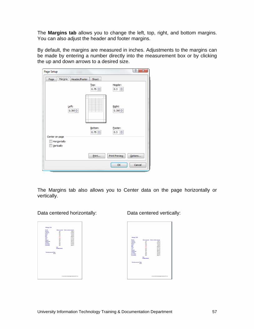
The Margins tab allows you to change the left, top, right, and bottom margins. You can also adjust the header and footer margins. By default, the margins are measured in inches. Adjustments to the margins can be made by entering a number directly into the measurement box or by clicking the up and down arrows to a desired size.

The Margins tab also allows you to Center data on the page horizontally or vertically. Data centered horizontally: Data centered vertically:


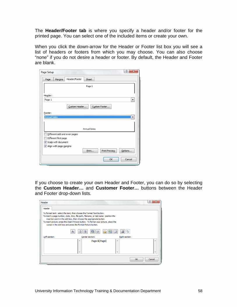
The Header/Footer tab is where you specify a header and/or footer for the printed page. You can select one of the included items or create your own. When you click the down-arrow for the Header or Footer list box you will see a list of headers or footers from which you may choose. You can also choose “none” if you do not desire a header or footer. By default, the Header and Footer are blank.

If you choose to create your own Header and Footer, you can do so by selecting the Custom Header… and Customer Footer… buttons between the Header and Footer drop-down lists.


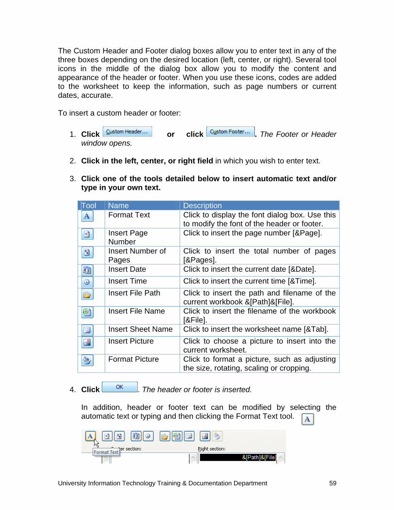
The Custom Header and Footer dialog boxes allow you to enter text in any of the three boxes depending on the desired location (left, center, or right). Several tool icons in the middle of the dialog box allow you to modify the content and appearance of the header or footer. When you use these icons, codes are added to the worksheet to keep the information, such as page numbers or current dates, accurate. To insert a custom header or footer:

1. Click or click . The Footer or Header window opens.

2. Click in the left, center, or right field in which you wish to enter text.

3. Click one of the tools detailed below to insert automatic text and/or

type in your own text.

Tool Name Description

Format Text Click to display the font dialog box. Use this

to modify the font of the header or footer.

Insert Page Number

Click to insert the page number [&Page].

Insert Number of Pages

Click to insert the total number of pages [&Pages].

Insert Date Click to insert the current date [&Date].

Insert Time Click to insert the current time [&Time].

Insert File Path Click to insert the path and filename of the

current workbook &[Path]&[File].

Insert File Name Click to insert the filename of the workbook

[&File].

Insert Sheet Name Click to insert the worksheet name [&Tab].

Insert Picture Click to choose a picture to insert into the

current worksheet.

Format Picture Click to format a picture, such as adjusting

the size, rotating, scaling or cropping.

4. Click . The header or footer is inserted.

In addition, header or footer text can be modified by selecting the automatic text or typing and then clicking the Format Text tool.


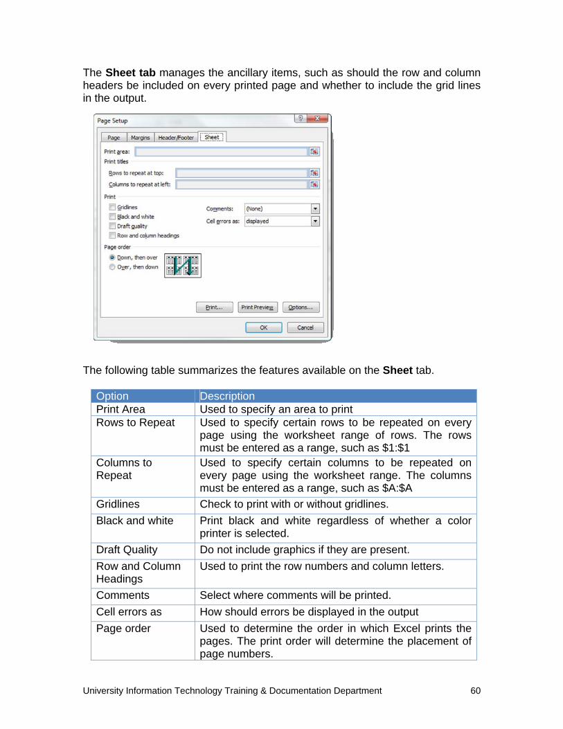
The Sheet tab manages the ancillary items, such as should the row and column headers be included on every printed page and whether to include the grid lines in the output.

The following table summarizes the features available on the Sheet tab.

Option Description Print Area Used to specify an area to print Rows to Repeat Used to specify certain rows to be repeated on every

page using the worksheet range of rows. The rows must be entered as a range, such as $1:$1

Columns to Repeat

Used to specify certain columns to be repeated on every page using the worksheet range. The columns must be entered as a range, such as $A:$A

Gridlines Check to print with or without gridlines.

Black and white Print black and white regardless of whether a color printer is selected.

Draft Quality Do not include graphics if they are present.

Row and Column Headings

Used to print the row numbers and column letters.

Comments Select where comments will be printed.

Cell errors as How should errors be displayed in the output

Page order Used to determine the order in which Excel prints the pages. The print order will determine the placement of page numbers.


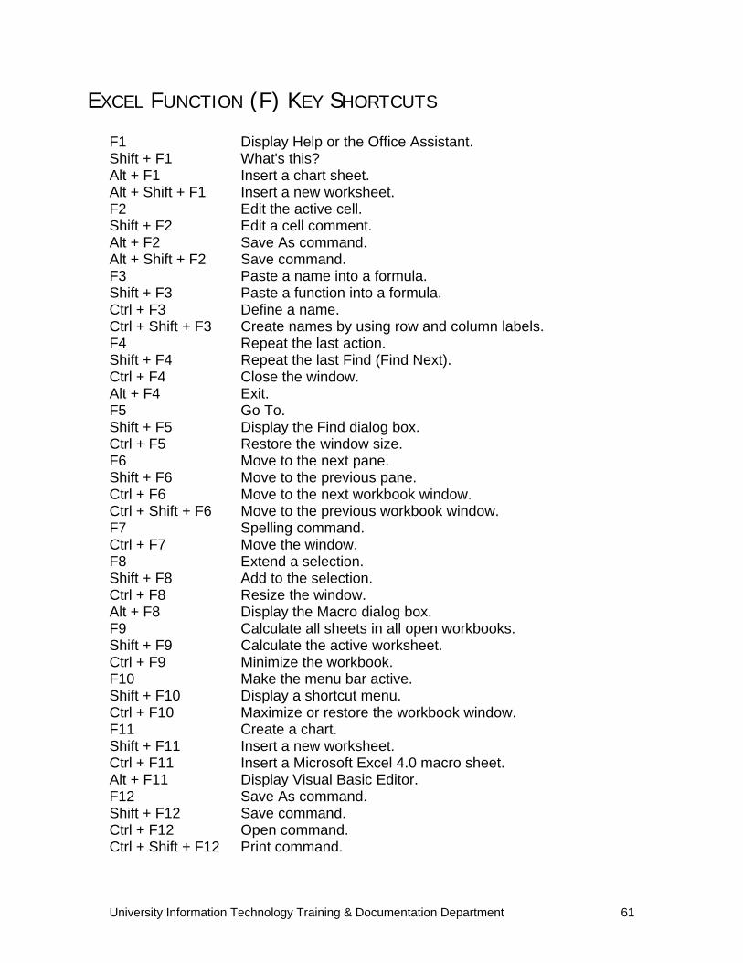
EXCEL FUNCTION (F) KEY SHORTCUTS F1 Display Help or the Office Assistant. Shift + F1 What's this? Alt + F1 Insert a chart sheet. Alt + Shift + F1 Insert a new worksheet. F2 Edit the active cell. Shift + F2 Edit a cell comment. Alt + F2 Save As command. Alt + Shift + F2 Save command. F3 Paste a name into a formula. Shift + F3 Paste a function into a formula. Ctrl + F3 Define a name. Ctrl + Shift + F3 Create names by using row and column labels. F4 Repeat the last action. Shift + F4 Repeat the last Find (Find Next). Ctrl + F4 Close the window. Alt + F4 Exit. F5 Go To. Shift + F5 Display the Find dialog box. Ctrl + F5 Restore the window size. F6 Move to the next pane. Shift + F6 Move to the previous pane. Ctrl + F6 Move to the next workbook window. Ctrl + Shift + F6 Move to the previous workbook window. F7 Spelling command. Ctrl + F7 Move the window. F8 Extend a selection. Shift + F8 Add to the selection. Ctrl + F8 Resize the window. Alt + F8 Display the Macro dialog box. F9 Calculate all sheets in all open workbooks. Shift + F9 Calculate the active worksheet. Ctrl + F9 Minimize the workbook. F10 Make the menu bar active. Shift + F10 Display a shortcut menu. Ctrl + F10 Maximize or restore the workbook window. F11 Create a chart. Shift + F11 Insert a new worksheet. Ctrl + F11 Insert a Microsoft Excel 4.0 macro sheet. Alt + F11 Display Visual Basic Editor. F12 Save As command. Shift + F12 Save command. Ctrl + F12 Open command. Ctrl + Shift + F12 Print command.

Aff Excel 2010

Documents

Transcript of Aff Excel 2010