1

Mathematical Programming Models and Solution Strategies for theSynthesis of Process Systems

Ignacio E. GrossmannCenter for Advanced Process Decision-making

Dept of Chemical Engineering,Carnegie Mellon University

Pittsburgh, PA 15213

PASI 2011Angra do Reis, R.J., Brazil

July 19-29, 2011

22

Sheppard, Socolow (2007)

- Sustainability and energy have recently emerged as key problems

Sustainability and Energy systems

33

Water scarcity

Design of Sustainable Processes requires Process Synthesis Techniques

4

Design: The creation of something in the mind.

Webster Dictionary

Design: a plan or drawing produced to show the look and function or workings of something before it is built or made

Oxford Dictionary

Design or Synthesis?

Synthesis: invention of new systems, configurations

Synthesis: the combination of components to form a connected whole

Oxford and Webster

Goal: Optimal Design

5

Major Areas: Process Systems Engineering

Oxygen

Air

Ethylene

Chlorine

Vinyl Chloride

Hydrogen Chloride

Ethylene Dichloride

Ethylene Dichloride

Water

Flash

Direct Chlorination

Oxychlorination

Low P

High P

Purge

Hydrogen Chloride

Design

t-1 t+1 t+kt ......

N

u(t+k|t)

y(t+k|t)

w(t+k|t)

t-1 t+1 t+kt ......

N

u(t+k|t)

y(t+k|t)

w(t+k|t)

t-1 t+1 t+kt ......

N

u(t+k|t)

y(t+k|t)

w(t+k|t)

t-1 t+1 t+kt ......

N

u(t+k|t)

y(t+k|t)

w(t+k|t)

t-1 t+1 t+kt ......

N

u(t+k|t)

y(t+k|t)

w(t+k|t)

t-1 t+1 t+kt ......

N

u(t)

w(t)

u(t+k|t)

y(t+k|t)

y(t)

w(t+k|t)

t-1 t+1 t+kt ......

N

u(t+k|t)

y(t+k|t)

w(t+k|t)

t-1 t+1 t+kt ......

N

u(t+k|t)

y(t+k|t)

w(t+k|t)

t-1 t+1 t+kt ......

N

u(t+k|t)

y(t+k|t)

w(t+k|t)

t-1 t+1 t+kt ......

N

u(t+k|t)

y(t+k|t)

w(t+k|t)

t-1 t+1 t+kt ......

N

u(t+k|t)

y(t+k|t)

w(t+k|t)

t-1 t+1 t+kt ......

N

u(t)

w(t)

u(t+k|t)

y(t+k|t)

y(t)

w(t+k|t)

t-1 t+1 t+kt ......

N

u(t+k|t)

y(t+k|t)

w(t+k|t)

t-1 t+1 t+kt ......

N

u(t+k|t)

y(t+k|t)

w(t+k|t)

t-1 t+1 t+kt ......

N

u(t+k|t)

y(t+k|t)

w(t+k|t)

t-1 t+1 t+kt ......

N

u(t+k|t)

y(t+k|t)

w(t+k|t)

t-1 t+1 t+kt ......

N

u(t+k|t)

y(t+k|t)

w(t+k|t)

t-1 t+1 t+kt ......

N

u(t)

w(t)

u(t+k|t)

y(t+k|t)

y(t)

w(t+k|t)

t-1 t+1 t+kt ......

N

u(t+k|t)

y(t+k|t)

w(t+k|t)

t-1 t+1 t+kt ......

N

u(t+k|t)

y(t+k|t)

w(t+k|t)

t-1 t+1 t+kt ......

N

u(t+k|t)

y(t+k|t)

w(t+k|t)

t-1 t+1 t+kt ......

N

u(t+k|t)

y(t+k|t)

w(t+k|t)

t-1 t+1 t+kt ......

N

u(t+k|t)

y(t+k|t)

w(t+k|t)

t-1 t+1 t+kt ......

N

u(t)

w(t)

u(t+k|t)

y(t+k|t)

y(t)

w(t+k|t)

t+Nt-1 t+1 t+kt ......

N

u(t+k|t)

y(t+k|t)

w(t+k|t)

t-1 t+1 t+kt ......

N

u(t+k|t)

y(t+k|t)

w(t+k|t)

t-1 t+1 t+kt ......

N

u(t+k|t)

y(t+k|t)

w(t+k|t)

t-1 t+1 t+kt ......

N

u(t+k|t)

y(t+k|t)

w(t+k|t)

t-1 t+1 t+kt ......

N

u(t+k|t)

y(t+k|t)

w(t+k|t)

t-1 t+1 t+kt ......

N

u(t)

w(t)

u(t+k|t)

y(t+k|t)

y(t)

w(t+k|t)

t-1 t+1 t+kt ......

N

u(t+k|t)

y(t+k|t)

w(t+k|t)

t-1 t+1 t+kt ......

N

u(t+k|t)

y(t+k|t)

w(t+k|t)

t-1 t+1 t+kt ......

N

u(t+k|t)

y(t+k|t)

w(t+k|t)

t-1 t+1 t+kt ......

N

u(t+k|t)

y(t+k|t)

w(t+k|t)

t-1 t+1 t+kt ......

N

u(t+k|t)

y(t+k|t)

w(t+k|t)

t-1 t+1 t+kt ......

N

u(t)

w(t)

u(t+k|t)

y(t+k|t)

y(t)

w(t+k|t)

t-1 t+1 t+kt ......

N

u(t+k|t)

y(t+k|t)

w(t+k|t)

t-1 t+1 t+kt ......

N

u(t+k|t)

y(t+k|t)

w(t+k|t)

t-1 t+1 t+kt ......

N

u(t+k|t)

y(t+k|t)

w(t+k|t)

t-1 t+1 t+kt ......

N

u(t+k|t)

y(t+k|t)

w(t+k|t)

t-1 t+1 t+kt ......

N

u(t+k|t)

y(t+k|t)

w(t+k|t)

t-1 t+1 t+kt ......

N

u(t)

w(t)

u(t+k|t)

y(t+k|t)

y(t)

w(t+k|t)

t-1 t+1 t+kt ......

N

u(t+k|t)

y(t+k|t)

w(t+k|t)

t-1 t+1 t+kt ......

N

u(t+k|t)

y(t+k|t)

w(t+k|t)

t-1 t+1 t+kt ......

N

u(t+k|t)

y(t+k|t)

w(t+k|t)

t-1 t+1 t+kt ......

N

u(t+k|t)

y(t+k|t)

w(t+k|t)

t-1 t+1 t+kt ......

N

u(t+k|t)

y(t+k|t)

w(t+k|t)

t-1 t+1 t+kt ......

N

u(t)

w(t)

u(t+k|t)

y(t+k|t)

y(t)

w(t+k|t)

t+Nt-1 t+1 t+kt ......

N

u(t+k|t)

y(t+k|t)

w(t+k|t)

t-1 t+1 t+kt ......

N

u(t+k|t)

y(t+k|t)

w(t+k|t)

t-1 t+1 t+kt ......

N

u(t+k|t)

y(t+k|t)

w(t+k|t)

t-1 t+1 t+kt ......

N

u(t+k|t)

y(t+k|t)

w(t+k|t)

t-1 t+1 t+kt ......

N

u(t+k|t)

y(t+k|t)

w(t+k|t)

t-1 t+1 t+kt ......

N

u(t)

w(t)

u(t+k|t)

y(t+k|t)

y(t)

w(t+k|t)

t-1 t+1 t+kt ......

N

u(t+k|t)

y(t+k|t)

w(t+k|t)

t-1 t+1 t+kt ......

N

u(t+k|t)

y(t+k|t)

w(t+k|t)

t-1 t+1 t+kt ......

N

u(t+k|t)

y(t+k|t)

w(t+k|t)

t-1 t+1 t+kt ......

N

u(t+k|t)

y(t+k|t)

w(t+k|t)

t-1 t+1 t+kt ......

N

u(t+k|t)

y(t+k|t)

w(t+k|t)

t-1 t+1 t+kt ......

N

u(t)

w(t)

u(t+k|t)

y(t+k|t)

y(t)

w(t+k|t)

t-1 t+1 t+kt ......

N

u(t+k|t)

y(t+k|t)

w(t+k|t)

t-1 t+1 t+kt ......

N

u(t+k|t)

y(t+k|t)

w(t+k|t)

t-1 t+1 t+kt ......

N

u(t+k|t)

y(t+k|t)

w(t+k|t)

t-1 t+1 t+kt ......

N

u(t+k|t)

y(t+k|t)

w(t+k|t)

t-1 t+1 t+kt ......

N

u(t+k|t)

y(t+k|t)

w(t+k|t)

t-1 t+1 t+kt ......

N

u(t)

w(t)

u(t+k|t)

y(t+k|t)

y(t)

w(t+k|t)

t-1 t+1 t+kt ......

N

u(t+k|t)

y(t+k|t)

w(t+k|t)

t-1 t+1 t+kt ......

N

u(t+k|t)

y(t+k|t)

w(t+k|t)

t-1 t+1 t+kt ......

N

u(t+k|t)

y(t+k|t)

w(t+k|t)

t-1 t+1 t+kt ......

N

u(t+k|t)

y(t+k|t)

w(t+k|t)

t-1 t+1 t+kt ......

N

u(t+k|t)

y(t+k|t)

w(t+k|t)

t-1 t+1 t+kt ......

N

u(t)

w(t)

u(t+k|t)

y(t+k|t)

y(t)

w(t+k|t)

t+Nt-1 t+1 t+kt ......

N

u(t+k|t)

y(t+k|t)

w(t+k|t)

t-1 t+1 t+kt ......

N

u(t+k|t)

y(t+k|t)

w(t+k|t)

t-1 t+1 t+kt ......

N

u(t+k|t)

y(t+k|t)

w(t+k|t)

t-1 t+1 t+kt ......

N

u(t+k|t)

y(t+k|t)

w(t+k|t)

t-1 t+1 t+kt ......

N

u(t+k|t)

y(t+k|t)

w(t+k|t)

t-1 t+1 t+kt ......

N

u(t)

w(t)

u(t+k|t)

y(t+k|t)

y(t)

w(t+k|t)

t-1 t+1 t+kt ......

N

u(t+k|t)

y(t+k|t)

w(t+k|t)

t-1 t+1 t+kt ......

N

u(t+k|t)

y(t+k|t)

w(t+k|t)

t-1 t+1 t+kt ......

N

u(t+k|t)

y(t+k|t)

w(t+k|t)

t-1 t+1 t+kt ......

N

u(t+k|t)

y(t+k|t)

w(t+k|t)

t-1 t+1 t+kt ......

N

u(t+k|t)

y(t+k|t)

w(t+k|t)

t-1 t+1 t+kt ......

N

u(t)

w(t)

u(t+k|t)

y(t+k|t)

y(t)

w(t+k|t)

t-1 t+1 t+kt ......

N

u(t+k|t)

y(t+k|t)

w(t+k|t)

t-1 t+1 t+kt ......

N

u(t+k|t)

y(t+k|t)

w(t+k|t)

t-1 t+1 t+kt ......

N

u(t+k|t)

y(t+k|t)

w(t+k|t)

t-1 t+1 t+kt ......

N

u(t+k|t)

y(t+k|t)

w(t+k|t)

t-1 t+1 t+kt ......

N

u(t+k|t)

y(t+k|t)

w(t+k|t)

t-1 t+1 t+kt ......

N

u(t)

w(t)

u(t+k|t)

y(t+k|t)

y(t)

w(t+k|t)

t-1 t+1 t+kt ......

N

u(t+k|t)

y(t+k|t)

w(t+k|t)

t-1 t+1 t+kt ......

N

u(t+k|t)

y(t+k|t)

w(t+k|t)

t-1 t+1 t+kt ......

N

u(t+k|t)

y(t+k|t)

w(t+k|t)

t-1 t+1 t+kt ......

N

u(t+k|t)

y(t+k|t)

w(t+k|t)

t-1 t+1 t+kt ......

N

u(t+k|t)

y(t+k|t)

w(t+k|t)

t-1 t+1 t+kt ......

N

u(t)

w(t)

u(t+k|t)

y(t+k|t)

y(t)

w(t+k|t)

t+N

Control

Operations

Plants MarketsDistribution

centers

SynthesisKey Problem

6

Process Synthesis

?

Phenomena to exploit?Equipment to implement?Interconnections?

Given inputs and desired outputs:

Inputs Outputs

The generation of process flowsheet alternatives(Rudd, Powers, Siirola, 1973)

7

Subsystems

- Heat exchanger network synthesis

- Separation systems: Distillation systems

- Reactor networks

- Reaction pathways

- Steam and Power plants

- Water networks, mass exchange networks

Process flowsheets

Basic representations

Basic methodologies

8

600

500

400

300

H1

H1 + H2

Min Heating 600KW

Min Cooling 2250kW

Composite Hot

C2

C1+C2

C1

Composite Cold

HRAT=20K PINCH!! (540-520)

Target min heating/min cooling

Pinch Analysis – Heat exchanger networks(Hohmann, Linnhoff)

9

A

BC

F

ABC

BC

BC-Azeo

Product Azeotrope

Mass BalanceDistillation Boundary

Distillation boundaries - Azeotropic Distillation

ABC

ABC

BC

AB

BC

A

B

B

Azeotrope

C

(Doherty, Perkins)

10

Attainable region - Reactor Networks(Glasser, Hildebrandt)

CSTR

PFR

11

• Evolutionary Search– Start with base case (Stephanopoulos, Westerberg)

• Systematic Generation– Means-Ends Analysis (Siirola, Powers)– Hierarchical decomposition (Douglas)

• Superstructure Optimization– NLP optimization (Sargent, Gaminibandara)– MINLP, Generalized Disjunctive Programming (Grossmann)

Subsystems and Process Flowsheets

12

Input-Output Level

Recycle System

Separation Synthesis

Heat Recovery

Batch vs Continuous

Hierarchical decompositionDouglas (1988)

13

Math Programming Approach to Process Synthesis

1. Develop a superstructure of alternative designs

2. Develop an NLP or (MINLP, GDP) model toselect topology and parameters of design

3. Solve NLP or (MINLP, GDP) model to extract optimumdesign embedded in superstructure

NLP = Nonlinear ProgrammingMINLP = Mixed-integer nonlinear programmingGBD = Generalized Disjunctive Programming

1414

Postulating superstructureCapturing all the alternativesUnderstanding implications for modeling

Model formulationPredicting performance: equationsCapturing logic: constraints

Solution algorithmExponential behavior due to combinatoricsOvercoming nonconvexities

Challenges

15

1

2

3

4

5

6

7

9

11

10

12

13

T1

T2

T3

T4

T5 T7

T8

T9

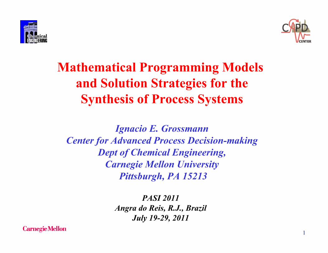
STATES: 1- A Raw, V, Low P 2- A mixed, V, Low P 3- A mixed, V,Low P to T3 4- A mixed, V,Low P to T4 5- A,V, High P form T3 6- A, V, High P form T4 7- A, V,High P, to preheat 8- A,V High P, High T 9- A ,V to packed reactor 10- A+B, V to mixer T10 11- A, V , to PFR

15 T12

T13

12- A+B, V to mixer T10 13- A+B, V to cooler 14- A+B, L to flash. 15- A+B, Rich in A, V, from purge splitter 16- A,V, low P 17- A+B, L, to distillation 18- B, L, Final Product 19- A, V, High P 20- A+B, V to purge 21- A+B, V, waste product

TASKS: 1- Mix recirc A and raw A 2- Split feed mixture 3- Compress in single stage 4- Compress in two stages 5- Mix compressed streams and recycle. 6- Preheat for reaction 7- Split to reactors 8- React A->B in the vapor phase in PFR

9- React A->B in vapor phase with catalizer C in packed reactor 10- Mix reactor outlets, Vapor 11- Condense stream 12- Flash A+B: A+B vapor, B liquid 13- Distillate A+B: A liquid, B liquid 14- Compress col. vapor outlet 15- Purge vapor stream

8T6 T10

T11

14

19

18

17T14 16

20

21

T15

state 19

task 14

State Task Network

•First step: State and Task Identification in process flowsheet.

Kondili, Pantelides, Sargent (1993)Yeomans, Grossmann (2000)

16

REACTOR 2:A-cat->B

COMPRESSOR 1

COMPRESSOR 2

FLASH

COLUMN

REACTOR 1:A-->B

PRE-HEATERCOOLER

FEED

PRODUCT

OTOE Assignment for STNPredetermined Equipment Assignment: One Task One Equipment

17

13

T11

141

2

3

4

5

6

7

9

11

10

12

T1

T2

T3

T4

T5 T7

T8

T9

20

T12

T13

8T6 T10

T1419

18

1716

15

21

T15

VTE Assignment for STN

Assignment left over for optimization: Variable Task Equipment

18

VTE:

Compress Recycle-or-Compress Feed

Equipment Tasks

Preheat feed to reactor-or-Cool reactor outlet-or-Vaporize recycle from distillation

React A-->B (liquid phase)-or-React A-cat->B in packedreactor (vapor phase)

1 stage 2 stage

state iequipment j

FEED

PRODUCT

State Equipment Network (SEN)

19

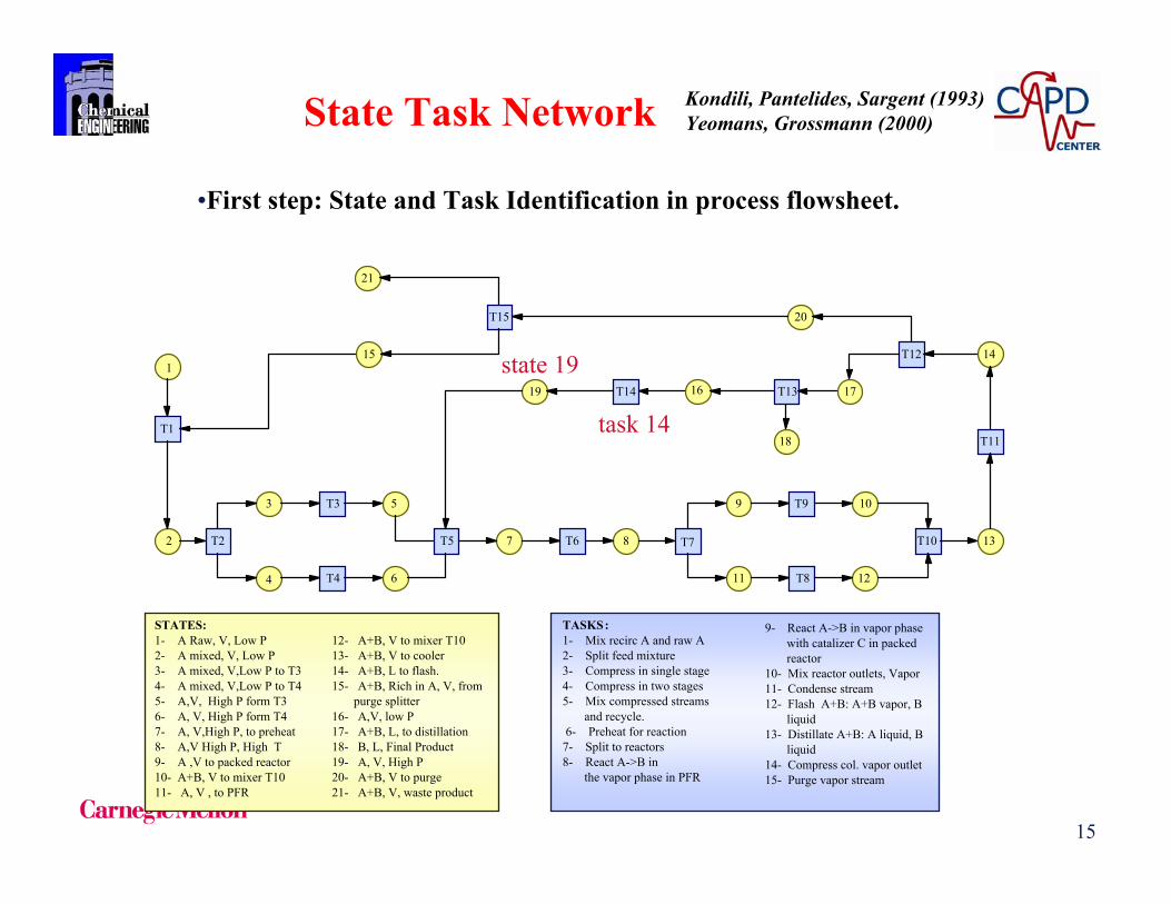
State-Space Superstructure Bagajewicz and Manousiouthakis (1992)

The inlet of each stream is denoted as a splitting node, and the outlet as a mixing node Each mass exchanger is identified by two splitting and mixing nodes, representing the rich and lean sides. Each storage tank is expressed as one splitting and mixing node.

Synthesis of mass exchanger networks for bach proceses

Li-Juan Li, Rui-Jie ZhouHong-Guang Dong (2010)

DistributionNetwork

Operators

2020

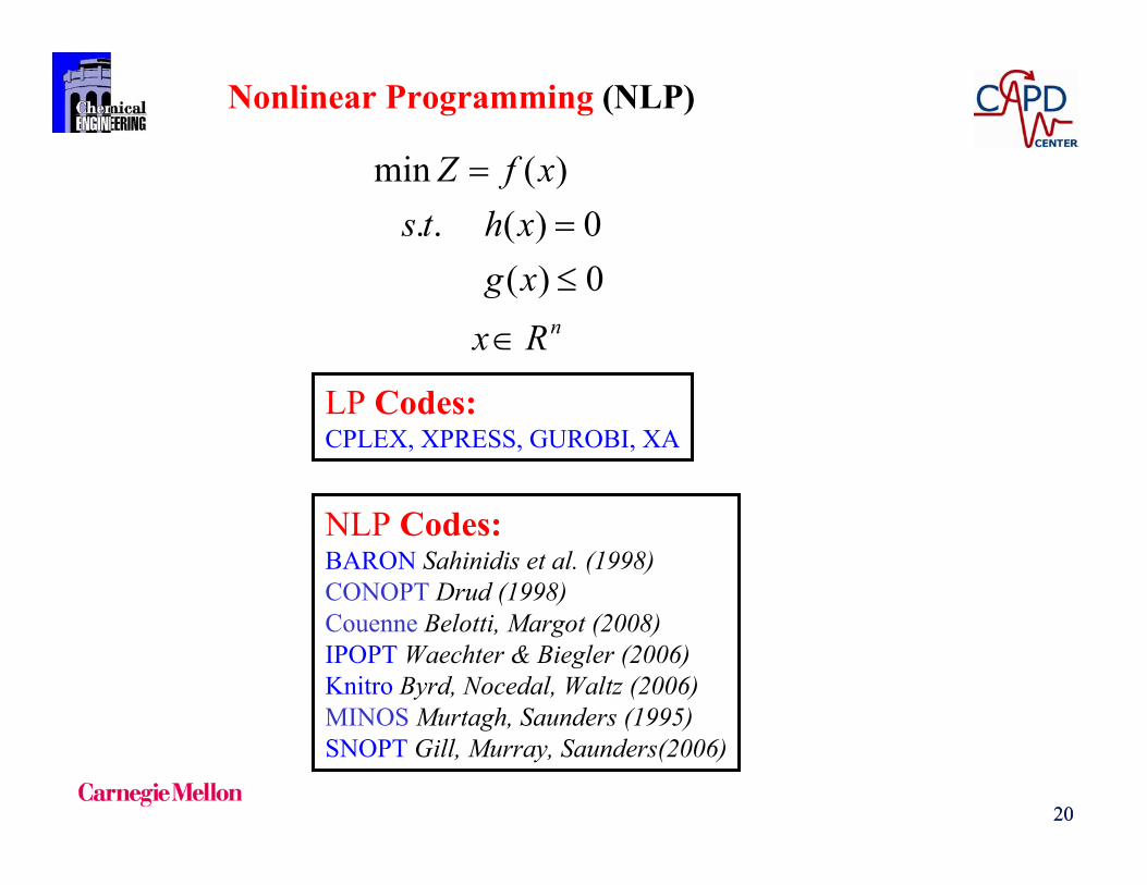
nRxxgx hts

xfZ

0)(0)( ..

)(min

Nonlinear Programming (NLP)

LP Codes:CPLEX, XPRESS, GUROBI, XA

NLP Codes:BARON Sahinidis et al. (1998)CONOPT Drud (1998)Couenne Belotti, Margot (2008)IPOPT Waechter & Biegler (2006)Knitro Byrd, Nocedal, Waltz (2006)MINOS Murtagh, Saunders (1995)SNOPT Gill, Murray, Saunders(2006)

2121

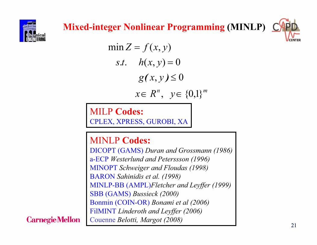
mn yRxyxgyx hts

yxfZ

1,0,0,

0),(..),(min

)(

Mixed-integer Nonlinear Programming (MINLP)

MILP Codes:CPLEX, XPRESS, GUROBI, XA

MINLP Codes:DICOPT (GAMS) Duran and Grossmann (1986)a-ECP Westerlund and Peterssson (1996)MINOPT Schweiger and Floudas (1998)BARON Sahinidis et al. (1998)MINLP-BB (AMPL)Fletcher and Leyffer (1999)SBB (GAMS) Bussieck (2000)Bonmin (COIN-OR) Bonami et al (2006)FilMINT Linderoth and Leyffer (2006)Couenne Belotti, Margot (2008)

2222

1

min

0

0

kk

jk

jkk

k jk

nk

jk

Z c f (x )

s.t. r(x )

Y

g (x ) k K j J

c γ

Ω Y true

x R , c RY true, false

Boolean Variables

Logic Propositions

Disjunctions

Generalized Disjunctive Programming (GDP)Raman, Grossmann (1994)

23

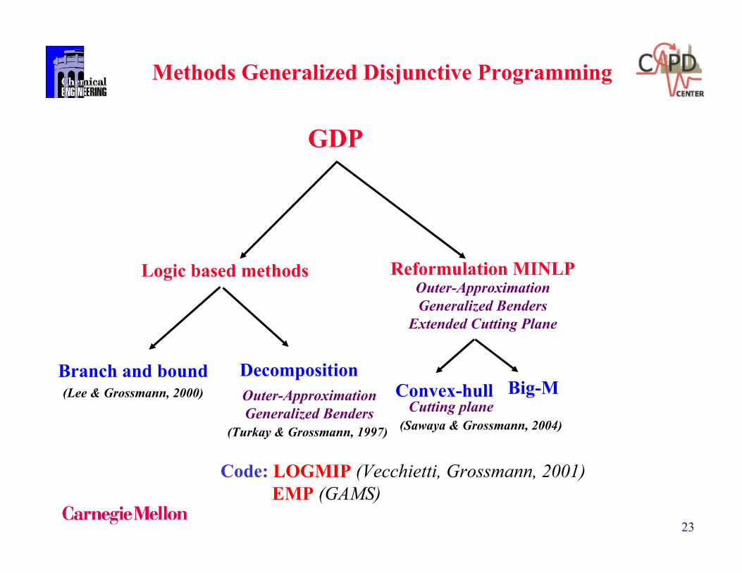
GDP

Logic based methods

Branch and bound(Lee & Grossmann, 2000)

DecompositionOuter-ApproximationGeneralized Benders

(Turkay & Grossmann, 1997)

Reformulation MINLPOuter-ApproximationGeneralized Benders

Extended Cutting Plane

Methods Generalized Disjunctive Programming

Convex-hull Big-MCutting plane

(Sawaya & Grossmann, 2004)

Code: LOGMIP (Vecchietti, Grossmann, 2001)EMP (GAMS)

2424

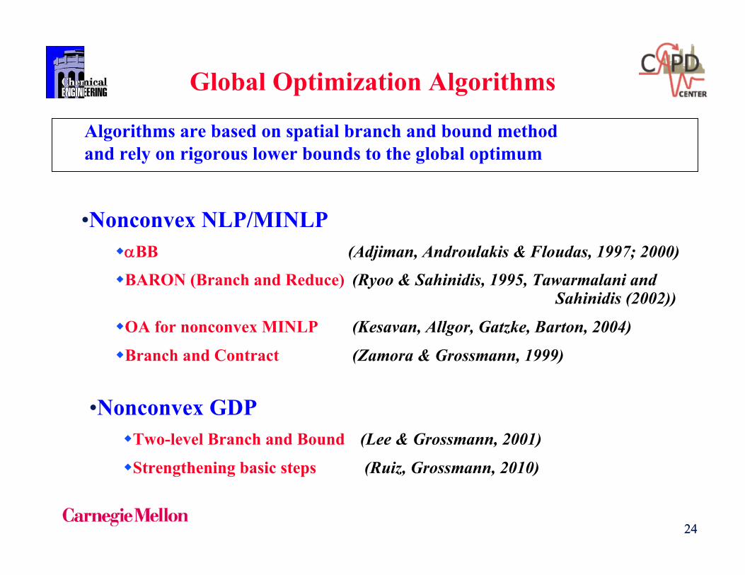
Global Optimization Algorithms

Algorithms are based on spatial branch and bound methodand rely on rigorous lower bounds to the global optimum

•Nonconvex NLP/MINLPBB (Adjiman, Androulakis & Floudas, 1997; 2000)

BARON (Branch and Reduce) (Ryoo & Sahinidis, 1995, Tawarmalani and Sahinidis (2002))

OA for nonconvex MINLP (Kesavan, Allgor, Gatzke, Barton, 2004)

Branch and Contract (Zamora & Grossmann, 1999)

•Nonconvex GDPTwo-level Branch and Bound (Lee & Grossmann, 2001)

Strengthening basic steps (Ruiz, Grossmann, 2010)

2525

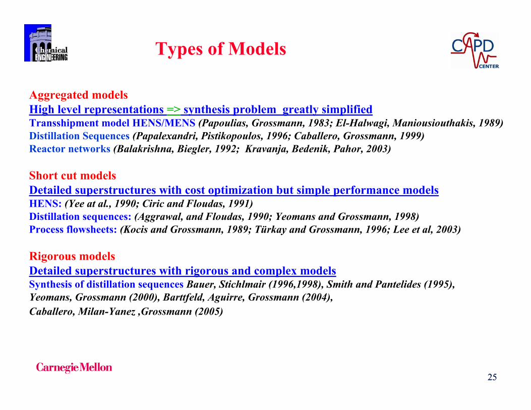
Types of Models

Aggregated models High level representations => synthesis problem greatly simplifiedTransshipment model HENS/MENS (Papoulias, Grossmann, 1983; El-Halwagi, Maniousiouthakis, 1989)Distillation Sequences (Papalexandri, Pistikopoulos, 1996; Caballero, Grossmann, 1999)Reactor networks (Balakrishna, Biegler, 1992; Kravanja, Bedenik, Pahor, 2003)

Short cut modelsDetailed superstructures with cost optimization but simple performance modelsHENS: (Yee at al., 1990; Ciric and Floudas, 1991)Distillation sequences: (Aggrawal, and Floudas, 1990; Yeomans and Grossmann, 1998)Process flowsheets: (Kocis and Grossmann, 1989; Türkay and Grossmann, 1996; Lee et al, 2003)

Rigorous models Detailed superstructures with rigorous and complex modelsSynthesis of distillation sequences Bauer, Stichlmair (1996,1998), Smith and Pantelides (1995), Yeomans, Grossmann (2000), Barttfeld, Aguirre, Grossmann (2004), Caballero, Milan-Yanez ,Grossmann (2005)

2626

1

2

3

4

5

6

H1

H2

H3

H4

C2

C1

QFuel

R 1

R 2

R 3

R 4

R 5

Q LP

Q HP

2000

1800

1000

800

3600

2000

2000

3500

2000

2000

3500

3500

47009000

9000

2500

2500

2500

4500

3000

14500

18000

Q CW

4700

10500

11600

5600

Aggregate Model: Transshipment Model for Heat Flows

Unknowns:a) Utility loadsQFuel, QHP, QLP, QCW

b) Heat residuals:R1,…R5

2727

Known parameters: heat contents of hot stream i and cold stream j in interval kcm, cn unit costs of hot utility m and cold utility n

Variables: heat loads of hot utility m and cold utility nRk heat residual exiting interval k

,H Cik jkQ Q

,S Wm nQ Q

HikQ C

jkQ

SmQ W

nQ

Rk-1

Rk

Interval k

LP transshipment model

1

1

min

0, 0, 00

k k k k

S Wm m n n

m S n W

S W H Ck k m n ik jk

m S n W i H j C

S Wk m n

K

C c Q c Q

st R R Q Q Q Q

R Q QR R

Linear Program

28

Fcp (MW/C) Tin(C) Tout(C) H1 1 400 120 H2 2 340 120 C1 1.5 160 400 C2 1.3 100 250

420 400 340 180 120

400 380 320 160 100

H1

H2

int 1

int 2

int 3

int 4

C1

C2

250

H1 H2 C1 C2

30 90 240 360

60 160 60 280

320 120 440

117 78 195

Heat contents (MW)Temperature intervals (K)

Example: 2 hot/2 cold

29

min Z = Qs + Qw s.t. R1 - Qs = -30 R2 - R1 = -30 R3 - R2 = 123 Qw - R3 = 102 Qs , Qw , R1 , R2 , R3 ≥ 0

Qs = 60 MW, Qw = 225 MW,R1 = 30 MW, R2 = 0, R3 = 123 MWR2 = 0 => pinch point at 340-320C

LP Transshipment:

30

Synthesis of Heat Exchanger NetworksYee and Grossmann (1990)

H1

H1-C1

H2

H1-C1

H1-C2

H2-C1

H2-C2

H1-C2

H2-C1

H2-C2

Stage k=1 Stage k=2

C1

C2

temperature location

k=1

temperature location

k=2

temperature location

k=3

H1,1tH1,2t

C1,1tC1,2t

C1,3t

H1,3t

H2,1t

H2,2tC2,1t C2,2t C2,3t

H2,3t

S1

S1

CW

CW

Multiple stages with potential heat exchangers zijk = 0,1

31

MINLP Model for Superstructure Optimization of Heat Exchanger Network Synthesis Yee and Grossmann (1990)

H1

H1-C1

H2

H1-C1

H1-C2

H2-C1

H2-C2

H1-C2

H2-C1

H2-C2

Stage k=1 Stage k=2

C1

C2

temperature location

k=1

temperature location

k=2

temperature location

k=3

H1,1tH1,2t

C1,1tC1,2t

C1,3t

H1,3t

H2,1t

H2,2tC2,1t C2,2t C2,3t

H2,3t

S1

S1

CW

CW

Two-stage superstructure

Parameters TIN = inlet temperature of stream TOUT = outlet temperature of stream F = heat capacity flow rate U = overall heat transfer coefficient CCU = unit cost for cold utility CHU = unit cost of hot utility CF = fixed charge for exchangers C = area cost coefficient B = exponent for area cost NOK = total number of stages = upper bound for heat exchange = upper bound for temperature difference Variables dtijk = temperature approach for match (i,j) at temperature location k dtcui = temperature approach for the match of hot stream i and cold utility dthuj = temperature approach for the match of cold stream j and hot utility qijk = heat exchanged between hot process stream i and cold process stream j in stage k qcui = heat exchanged between hot stream i and cold utility qhuj = heat exchanged between hot utility and cold stream j ti,k = temperature of hot stream i at hot end of stage k tj,k = temperature of cold stream j at hot end of stage k zijk = binary variable to denote existence of match (i,j) in stage k zcui = binary variable to denote that cold utility exchanges heat with stream i zhuj = binary variable to denote that hot utility exchanges heat with stream j

32

AssumptionIsothermal mixing => linear constraints

tik tik+1

qijk

zijk=0,1

Procedure1. Solve MINLP assuming isothermal mixing2. If splitting streams, solve NLP on reduced final configuration

Rigorous if no stream splits

No. stages: max no. hot, no. cold

33

Overall heat balance for each stream

j j j ijk jk ST i HP

(TOUT - TIN ) F = q +qhu j CP

i i i ijk ik ST j CP

(TIN - TOUT ) F = q +qcu i HP

Heat balance at each stage

,i,k i,k+1 i ijkj CP

(t - t ) F = q i HP k ST

,j,k j,k+1 j ijkj HP

(t - t ) F = q j CP k ST

Feasibility of temperaturesti,k ti,k+1 kST, iHPtj,k tji,k+1 kST, jCPTOUTi ti,NOK+1 iHPTOUTj tj,1 jCP

Hot and cold utility load(ti,NOK+1 - TOUTi) Fi = qcui iHP(TOUTj - tj,1) Fj = qhuj jCP

34

Logical constraintsqijk - zijk 0 iHP, jCP, kSTqcui - zcui 0 iHPqhuj - zhuj 0 jCPzijk, zcui, zhuj = 0,1

Calculation of approach temperaturesdtijk ti,k - tj,k + (1 - zijk) kST, iHP, jCPdtijk+1 ti,k+1 - tj,k+1 + (1 - zijk) kST, iHP, jCPdtcui ti,NOK+1 - TOUTCU + (1 - zcui) iHP

dthui TOUTHU - tj,1 + (1 - zhuj) jCPdtijk EMAT

Objective functionChen approximation (1987)

LMTD ~ [(dtl*dt2)*(dtl+dt2)/2]1/3

, ,

1/31 1

min

... .[( )( )( ) / 2)]

i ji HP j CP

ij ijk i CU i i HU ji HP j CP k ST i HP j CP

ij ijk

i HP j CP k ST ijk ijk ijk ijk ijk

Z CCUqcu CHUqhu

CF z CF zcu CF zhu

C qetc

U dt dt dt dt

SYNHEAT: http://newton.cheme.cmu.edu/interfaces

35

*PROCESS STREAMS*

*HOT:TIIN.FX('1') = 480.00;TIOUT.FX('1') = 340.00;FCI('1') = 1.50;CFI('1') = 1.00;

TIIN.FX('2') = 420.00;TIOUT.FX('2') = 330.00;FCI('2') = 2.00;CFI('2') = 1.00;

*COLD:TJIN.FX('1') = 320.00;TJOUT.FX('1') = 410.00;FCJ('1') = 1.00;CFJ('1') = 1.00;

TJIN.FX('2') = 350.00;TJOUT.FX('2') = 460.00;FCJ('2') = 2.00;CFJ('2') = 1.00;

TMAPP = 10.00;

*UTILITIES*CFHU = 1.00;THUIN = 500.00;THUOUT = 500.00;CFCU = 1.00;TCUIN = 300.00;TCUOUT = 300.00;

**COSTS**UTILITIESHUCOST = 80.00;CUCOST = 20.00;

UNITC = 1000.00;ACOEFF = 20.00;HUCOEFF = 20.00;CUCOEFF = 20.00;

36

480.0 340.0

420.0 330.0

1.5

2.0

420.0 360.0

360.0

H 1

H 2

90.0 kW 90.0 kW

120.0 kW

11.0 m2

8.3 m2

23.9 m2

W

W

S

30.0 kW

60.0 kW

10.0 kW

320.0 410.0

350.0 460.0

1.0

2.0

455.0 410.0

C 1

C 2

Total Network Cost ($/yr) = 8962.60

37

320

340

360

380

400

420

440

460

480

0 50 100 150 200 250 300 350 400 450

T (K

)

Q (kW)

SYNHEAT: T-Q CURVE

38

Hot streams

Qa) Sensible heat

i i i iQ FCp TIN TOUT

Qb) Isothermal

condi iQ F

Qc) Sensible and latent heat

suph cond condi i i i i

subc condi i i

Q FCp TIN T F

FCp T TOUT

superheated

saturatedsubcooled

Cold streams

Qd) Sensible heat

j j j jQ FCp TOUT TIN

Qe) Isothermal

evapj jQ F

Qf) Sensible and latent heat

suph evap evapj j j j j

subc evapj j j

Q FCp TOUT T F

FCp T TIN

superheated

saturatedsubcooled

Set HPS1 Set HPS2 Set HPS3

Set CPS1 Set CPS2 Set CPS3

TIN

TIN

TIN

TIN

TIN

TIN

TOUT

TOUT

TOUT

TOUT

TOUT

TOUT

Extension to isothermal streams in the MINLP ModelPonce-Ortega, J.M., A. Jiménez and I.E. Grossmann (2008)

Different cases modeled with disjunctions

39

•Feasibility of Latent Heat Exchange

1 1, ,

, 1 , 1

, ,0 0

i k i k

cond condi k i i k i

i k i k

Y Y

t T t Tq q

, 0i kq

1,i kY1

,i kY

, 0i kq

3i HPS,i kt , 1i kt

Outlet temperature for hot stream

Example of disjunctive constraint

40

Ref: Bruno et al. (1998)

Superstructure for Utility Plants

41

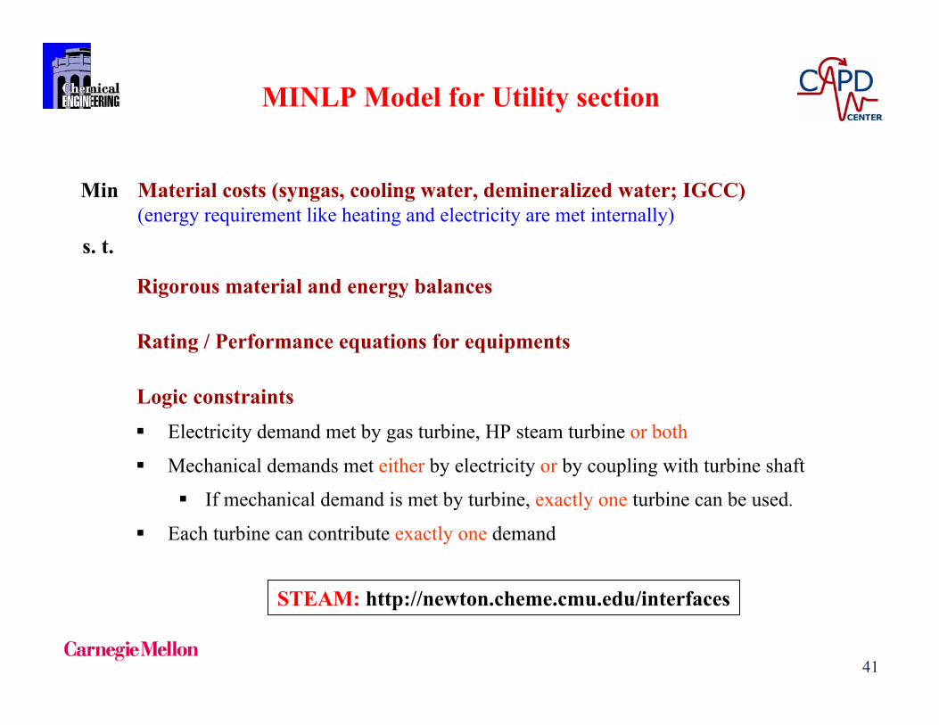
Min Material costs (syngas, cooling water, demineralized water; IGCC)(energy requirement like heating and electricity are met internally)

s. t.

Logic constraints

Rigorous material and energy balances

Electricity demand met by gas turbine, HP steam turbine or both

Mechanical demands met either by electricity or by coupling with turbine shaft

If mechanical demand is met by turbine, exactly one turbine can be used.

Each turbine can contribute exactly one demand

Rating / Performance equations for equipments

MINLP Model for Utility section

STEAM: http://newton.cheme.cmu.edu/interfaces

42

Electricity: 500 MWMechanical Power No 1: 5 MWMechanical Power No 2: 15 MWHP Heating: 5 MWMP Heating: 20 MWLP Heating: 50 MW

Demands Pressure of Steam HeadersHP: 45 barMP: 20 barLP: 7 bar

62 process streams3 HP turbines (7 modes)2 MP turbines (3 modes)5 Headers (HP, MP, LP, Cond, Vac)1 Gas turbine (compressor, expander)3 Boilers (HP, MP, HRSG)4 Combustors (GT, Boilers)5 Liquid pumps2 Air blowers1 Deaerator

Superstructure

Non-convex MINLP problem Binary variables: 44Continuous variables: 1275Constraints: 1309

Modeled and solved using GAMS/DICOPT(Intel Core 2 Duo 2.4 GHz with 2 GB RAM)

Numerical Example for Utility Model

43

Operating cost = $307.27 Million/yr

Optimal Solution for Numerical Example

44

Carnegie Mellon

Water-using unit 1

Water-using unit 1

Water-using unit 2

Water-using unit 2

Water-using unit 3

Water-using unit 3

Raw Water Raw Water TreatmentRaw Water Treatment

Boiler Feedwatertreatment

Boiler Feedwatertreatment

Steam SystemSteam System

WastewaterBoiler Blowdown

SteamCondensate Losses

Boiler

Freshwater Wastewater

Cooling Tower

Cooling Tower Blowdown

Water Loss by Evaporation

Discharge

Wastewater TreatmentWastewater Treatment

StormWater

Other Uses(Housekeeping)

Other Uses(Housekeeping)

Wastewater

ConventionalSystem

45

Carnegie Mellon

• Given is: – a set of single/multiple water sources with/without contaminants, – a set of water-using, water pre-treatment, and wastewater

treatment operations, sinks and sources of water

• Synthesize an integrated process water network– interconnection of process and treatment units (reuse, recycle)– the flow rates and contaminants concentration of each stream– minimum total annual cost of water network

Approach: Global NLP or MINLP superstructure optimization model

Synthesis of Integrated Process Water Networks

Synthesis Integrated Process Water Networks• Pinch analysis and mathematical programming models• Reviews in Bagajewicz (2000), Ježowski (2008), Bagajewicz and Faria (2009), and Foo (2009).

46

Carnegie Mellon

Superstructure for water networks for water reuse, recycle, treatment, and with sinks/sources water

Freshwater

Process Unit

Treatment Unit

Sink

Source

Ahmetovic, Grossmann (2010)

Main features:- Multiple feeds- Source/Sink units- Local recycles- All possible interconnections

-Fixed and variable flows through process units

47

Precipitation

Total suspe. solids

Organiccomp.

HeavyMetals

Inorgan. salts

Organicnot BT

Heavymetals

Sedimentation

Filtration

Flotation

Ultrafiltration

Reverse Osmosis

IonicExchange

Evaporation

Adsortion Aerobic

Oxidation Anaerobic

Bio. Sulphate

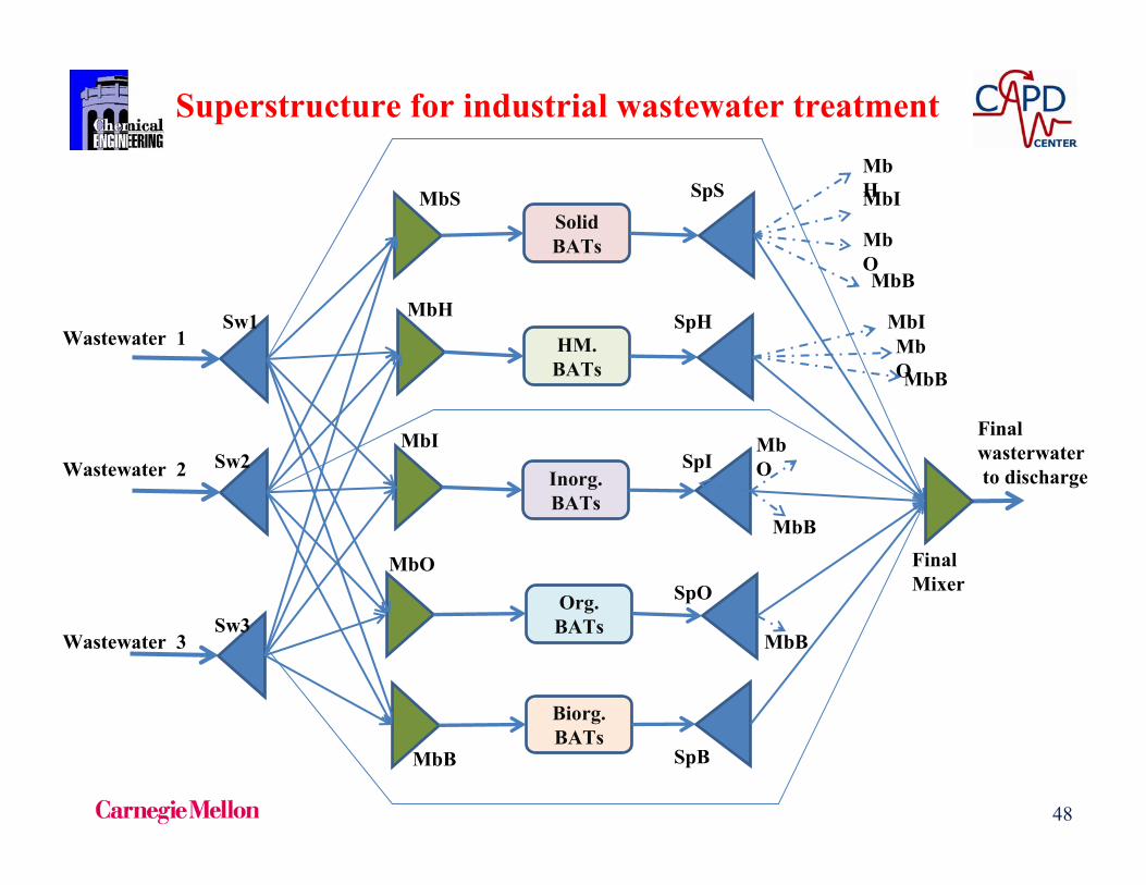
Industrial wastewater requires complex treatment networks

Sequential treatment has been chosen with 2-4 Best Available Technologies for the removal of each type of pollutant

Note on Treatment Units Galan, Grossmann (2011)

48

SolidBATs

HM. BATs

Inorg. BATs

Org. BATs

Biorg. BATs

MbS

MbH

MbI

MbO

MbB

SpS

SpB

SpO

SpI

SpH

Final Mixer

Wastewater 1

Wastewater 2

Wastewater 3Sw3

Sw1

Sw2Final wasterwaterto discharge

MbH

MbB

MbO

MbI

MbIMbOMbB

MbB

MbB

MbO

Superstructure for industrial wastewater treatment

49

Carnegie Mellon

Objective function: min Cost

Subject to:Splitter mass balances Mixer mass balances (bilinear)Process units mass balancesTreatment units mass balances Design constraints

Nonconvex NLP or MINLP

Optimization Model

0-1 variables for piping sections

Model can be solved to global optimality

50

Carnegie Mellon

SWsFITFIDFIPFIFFWTUt

tsDUd

dsPUp

psss

,,,

Splitter

linear SWsyFIFFIFyFIFss FIF

UssFIF

Ls

PUpSWsyFIPFIPyFIPpsps FIP

UpspsFIP

Lps ,

,, ,,,

DUdSWsyFIDFIDyFIDdsds FID

UdsdsFID

Lds ,

,, ,,,

TUtSWsyFITFITyFITtsts FIT

UtstsFIT

Lts ,

,, ,,,

0-1optional

bilinear if the flow treated as cont. variable

PUpFPFPFIPFTPFSPFPU

pp RPUp

pp

RppPUp

ppSWs

psTUt

ptSUr

prinp

,1

','

0,''

,',,,

jPUpxSPUFPxSPUFP

xWFIPxSTUFTPxSUFSPxPUFPU

outjp

RPUp

ppout

jp

RppPUp

pp

injs

SWsTUt

outjtpt

outjr

SUrpr

injp

inp

pp

,,,'

1'

,','

0,''

,'

,,,,,,

Mixer

bilinear

PUpFPUFPU outp

inp

jPUpxPUFPULPUxPUFPU outjp

outpjp

injp

inp ,10 ,

3,,

linear if flowrate is fixed

Process unit

51

Carnegie Mellon

TUt

outtt

TUt

outtts

SWss FTUOCHFTUICARCFWFWHZ min

Cost function linear in feedwater, concave in treatment unit, linear in operating cost, pipe section fixed charge (0-1)

52

Carnegie Mellon

Controlling complexity network

max

1'

0,''

1'

0,''

,,

,,,,

,,',',

,',',,

Nyy

yyyyy

yyyyy

yyyyyy

SUr PUpFSP

SUr TUtFST

SUrFSO

SUr DUdFSD

TUt DUdFTD

PUp DUdFPD

SWs DUdFID

TUt PUpFTP

TUtFTO

RTUt TUt

FT

RttTUt TUt

FTPUp TUt

FPT

RPUp PUp

FPOPUp

FP

RppPUp PUp

FPSWs

FIFSWs TUt

FITSWs PUp

FIP

prtr

rdrdtdpds

ptt

t

tt

t

tttp

PU

ppp

p

ppstsps

Limit number of 0-1 vars to Nmax number “removable” pipes

Can develop trade-off curve solving successive MINLPs

Cost

Nmax

53

Carnegie Mellon

Convexification of Non-convex functions

iLj

iUiiLj

ij

iUij

iUj

iLiiUj

ij

iLij

iUj

iUiiUj

ij

iUij

iLj

iLiiLj

ij

iLij

CFFCCFf

CFFCCFf

CFFCCFf

CFFCCFf

McCormick (1976 )

Under- and over-estimators ( Linear Inequalities )

FiL ≤ Fi ≤ FiU CjiL ≤ Cj

i ≤ CjiU

C

CL

FL

CU

FU

F

Underestimators

Overestimators

Bilinear term

Convex Envelopes for Bilinear Terms F*C

Underestimation of Concave functions

F

(FL)

FL

(FU)

FU

F

Underestimator

Concave term

iLiiLiU

iLiUiLi

FFFFFFFF

FiL ≤ Fi ≤ FiU

( Secant line )

54

Carnegie Mellon

bilinear terms for the treatment units and final mixing points

jxDUFDUxF

xTUFTUxSUFSULPUxWFW

injd

DUd

ind

outj

out

injt

TUt

intjtTU

outjr

SUr

outr

PUpjp

injs

SWss

,

,,,3

,, )1(10

Cut is redundant for original problem Non-redundant for relaxation problem

•The cut proposed by Karuppiah and Grossmann (2006) is incorporated to significantly improve the strength of the lower bound for the global optimum: contaminant flow balances for the overall water network system

•Tight bounds on the variables are expressed as general equationsobtained by physical inspection of the superstructure and using logic specifications

WATER: http://newton.cheme.cmu.edu/interfaces

55

Carnegie Mellon

Unit Flow rate (t/h) Discharge load(kg/h)

Maximum inletconcentration (ppm)

A B A BPU1 40 1 1.5 0 0PU2 50 1 1 50 50

Unit % Removal for contaminant

IC (Investment cost coefficient)

OC (Operating cost coefficient)

α

A BTU1 95 0 16800 1 0.7TU2 0 95 12600 0.0067 0.7

Data of process units.

Data of treatment units.

The objective of this example is to:- solve NLP and MINLP water network problems -compare results obtained with/without allowed recycle around process units- illustrate how the complexity of the water networks can be controlled

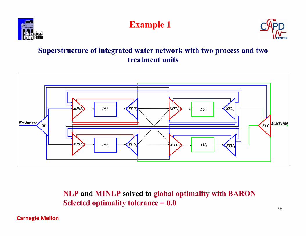
Example 1

56

Carnegie Mellon

Superstructure of integrated water network with two process and two treatment units

Example 1

NLP and MINLP solved to global optimality with BARONSelected optimality tolerance = 0.0

57

Carnegie Mellon

Continuous

variables

Discrete

variables

Constraints CPU time

(s)

55 - 44 < 0.5

57* - 44 < 1.0

75 20 85 < 3.6

79*

77**

22

20

89

85

< 2.5

13.2*Option with local recycles. **Variable flowrates in process units.

Model statistics and computational results for Example 1

58

Carnegie Mellon

Without recycle With recycleFreshwater cost $320000 $320000Investment cost on treatment units $37440 $33585.3Operating costs for treatment units $238723.6 $230431.6Total cost $596163.6 $584016.9

Without recycle With recycleFreshwater cost $320000 $320000Investment cost on pipes $540.69 $546.3Operating cost for pumping water $10056.26 $9427.84Investment cost on treatment units $37440.01 $33585.32Operating costs for treatment units $238723.59 $230431.64Total cost $606760.55 $593991.1

Case 1 (NLP): Objective function: cost of water, investment cost on treatment units and operating cost for treatment units

Case 2 (MINLP): Objective function: cost of water, investment cost on treatment units, operating cost for treatment units, investment cost on pipes, operating cost for pumping water through pipes

Example 1

2% saving with recycle

59

Carnegie Mellon

Optimal solution for the NLP and MINLP problem without local recycle

8 “removable connections”

Optimal solution for the NLP and MINLP problem with local recycle9 “removable connections”

60

Carnegie Mellon

Pareto-optimal solutions for minimum cost and minimum number of removable connections

61

Carnegie Mellon

Objective of this example: show that proposed model can be used to establish trade-off complexity vs cost of water network

Unit Flow rate (t/h) Discharge load(kg/h)

Maximum inletconcentration (ppm)

A B C A B CPU 1 40 1 1.5 1 0 0 0PU 2 50 1 1 1 50 50 50PU 3 60 1 1 1 50 50 50PU 4 70 2 2 2 50 50 50PU 5 80 1 1 0 25 25 25

Unit Removal ratio (%) IC (Investment cost coefficient)

OC (Operating cost coefficient)

α

A B CTU 1 95 0 0 16800 1 0.7TU 2 0 0 95 9500 0.04 0.7TU 3 0 95 0 12600 0.0067 0.7

Data for process units

Data for treatment units

Example 2

62

Carnegie Mellon

Superstructure of the integrated water network

MINLP: 72 0-1 vars, 233 cont var, 251 constroptcr=0.01 197.5 CPUsec

63

Carnegie Mellon

Cost of water network for different number ofremovable piping connections

Example 2

Note: reduction 7 pipe segments => 28 % increase in cost

64

Carnegie Mellon

Optimal design of the simplified water network with 13 removable connections

65

Carnegie Mellon

Large scale water network problem4 feeds, 6 process units, 4 treatment units, 3 contaminants

NLP: 232 variables, 121 constraints BARON: 2 secs

Optimal FreshwaterConsumption

40 t/hvs

390 t/hconventional

Advantage Simultaneous vs SequentialLeads to total lower cost and higher overall conversion

Energy &water cost (simultaneous)

66

Energy &water cost (sequential)

Total cost (sequential)

Cost

Overall conversion

raw material cost

Total cost (simultaneous)

Simultaneous heat and water flowsheet optimization

Flowsheets with recycle

HEAT TARGETING

PROCESS FLOWSHEET

WATER TARGETING

Cold streams

Hot streams

MUC*

*MUC – minimum utility consumption

Hot utility

Cold utility

MUC*Water streams

Wastewater

Freshwater

Utility networks

PROCESS STRUCTURE

WN STRUCTURE HEN STRUCTURE

PROCESS FLOWSHEET WITH HEN AND WN67

Strategy for simultaneous optimizationDuran, Grossmann (1986) Yang, Grossmann (2011)

68

Carnegie Mellon

T (K)500

400

300

Q (kW)

Qs = 35H1

Qw = 145H1

500

400

300

Qs = 10H1

Qw = 120H1

(a) Pinch candidate H1 (b) Pinch candidate H2

(c) Pinch candidate C1 (d) Pinch candidate C2

500

400

300

Qs = -110C1

Qw = 0C1

500

400

300

Qs = - 80C2

Qw = 30C2

Target Minimum Utility CostPinch Location Method Duran, Grosmann (1986)

Basic idea: Assume pinch occurs at every inlet and determine maximum heating

69

Carnegie Mellon

m i n C = f(x) + cSQS + cWQW s . t . h(x) = 0 g(x) 0

Q S fj max 0, t j

out - Tp - Tmin j =

n C - max 0, t j

in - T p - T min

- F i max 0, Ti

in -Tp - max 0, Tiout -Tp

i =

n H

Q W = Q S + Fi Ti

in - Tiout - f j t j

out - t jin

j=

nC

i=

nH

Q S , Q W 0, Fi 0 i = 1... n H, fj

0 j = 1... n C x Rn

p P

where Tp, p P Pinch Candidate

Heat balance above pinch point for heating utility

Total heat balance for cooling utility

LP targeting model (parametric in flows, temperatures)

Min obj plus cost heating and cooling

Heatintegrationconstraints

70

Carnegie Mellon

PRODUCT D

FEEDA, B

inert C

H C

H

H

A+B DREACTOR

FLASH

steam

PURGEC1

C3

H1, H2*C2

H3C

*H1 superheat to dew point H2 dew point to supercool

3 hot process streams 3 cold process streams

Example Simultaneous Optimizationand Heat Integration

Optimize operating conditions of flowsheet while integratinghot and cold streams to minimize utility cost

71

Carnegie Mellon

ECONOMIC Expenses (x 106 $ / yr): Feedstock 22.6717 26.4166 Capital investment 3.7596 3.9108 Electricity compress 2.3774 2.4871 Heating utility 2.8244 14.4586 Cooling utility 0.7900 0.7247 Earnings (x 106 $ / yr): Product 41.5300 41.5300 Purge 4.5169 6.8242 Generated steam 5.6407 9.7441 Annual Profit 19.2645 90% HIGHER! 10.1005 TECHNICAL Overall conversion A 81.68 75.13 [ % ] Pressure reactor 12.10 13.87 [atm] Conversion per pass 30.43 37.53 [ % ] Temp. inlet reactor 450.00 450.00 [ K ] Temp. outlet reactor 502.65 450.00 [ K ] Steam generated 10119.12 17479.60 [ kW ] Pressure in flash 9.10 10.87 [atm] Temperature flash 320.00 339.88 [ K ] Purge rate 9.66 19.66 [ % ] Power compressors 11353.60 11877.44 [ kW ] Heating utility 1684.27 8622.04 [ kW ] Cooling utility 10632.04 9752.77 [ kW ] Total heat exchanged 31962.20 28720.61 [ kW ]

Simultaneous Sequential

Higher profit

Higher conversion

72

Carnegie Mellon

200

300

500

700

10,000 20,000 30,000 40,000 H (kW)5,0002,000

T (K)

Q = 1, 684H

DTmin = 15 K

inlet H1

HOT

COLDpinch

(502.7, 487.7)

pinch (383.7, 368.7)

inlet C2Qc = 10, 632

SIMULTANEOUS

(Total Heat exchanged = 31, 962 kW)

200

300

500

700

10,000 20,000 30,000 40,000 H (kW)5,0002,000

T (K)

Q = 8, 622H

DTmin = 15 K

HOT

COLD

pinch (363.1, 348.1)

inlet H2

Qc = 9, 753

SEQUENTIAL

(Total Heat exchanged = 28, 720 kW)

Simultaneous optimizationLower heating

Sequential optimizationHigher heating

73

Carnegie Mellon

outin

kj

pkpj

ij

piin

pout

iout

pin

kinout

ij

kj

insi

ik

outmi

iUji

kUjk

outmi

ik

pkpiPUpjCGainFLCLossF

piPUpPFpkPUpPF

sksiSUsjCC

skSUsFF

mkMUmjCFCF

mkMUmFF

out

in

in

,,,)()(

,,

,,

,

,,

,s.t.

,

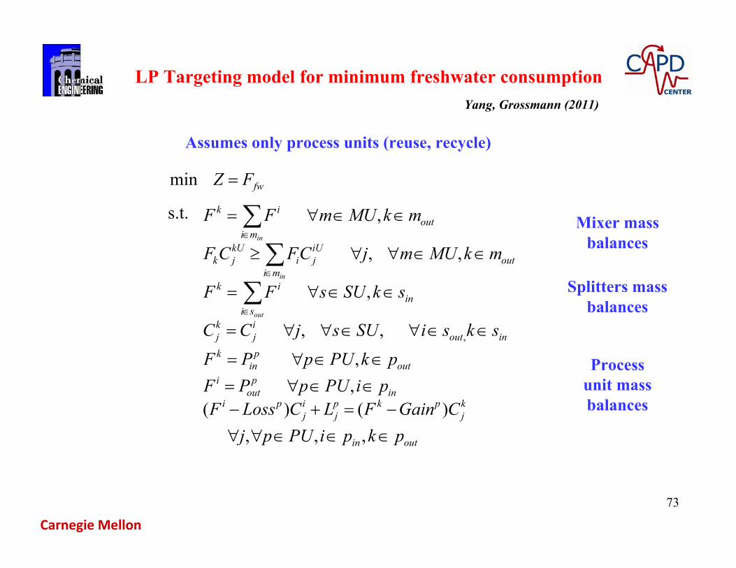
fwFZ min

Splitters mass balances

Process unit mass balances

Mixer mass balances

LP Targeting model for minimum freshwater consumption

Assumes only process units (reuse, recycle)

Yang, Grossmann (2011)

74

Carnegie Mellon

VvUuXxFWvg

QQugvuxg

vuxh

FWcQcQcvuxF

WNCH

HEN

P

fwCUj

jC

jC

HUi

iH

iH

,,0),(

0),,( 0),,(

0),,( s.t.

),,(.min

Process flowsheet constraints

Heat targeting constraints

Water targeting constraints

Design parametersP, V, T, F

Heat integration parametersFi, Ti

in, Tiout

Water integration parameters

Simultaneous optimization, heat and water integration

Utility cost Freshwater cost

75

Carnegie Mellon

+ cooling system+ steam system

Freshwater requirement

Heating requirement

Cooling requirement

methanol synthesis from syngas

Simultaneous optimization, heat and water integration

76

SEQUENTIAL SIMULTANEOUS

Profit (1000 $/yr) 62,695 73,416Investment cost (1000 $) 1,891 1,174Operating costs and parameters

electricity (KW) 6.59 1.84freshwater (kmol/s) 202.4 162.5

heating utility (10^9 KJ/yr) 0.29 0cooling utility (10^9 KJ/yr) 67.3 72.7

Steam generated (10^9 kJ/yr) 2448 1965overall conversion 0.23 0.29

Material flowrate (10^6 kmol/yr)feedstock 48.04 37.13

product 10.89 10.89byproduct 9.95 4.41

17% improvement in profit

* Solved with BARON

Sequential vs simultaneous comparison

77

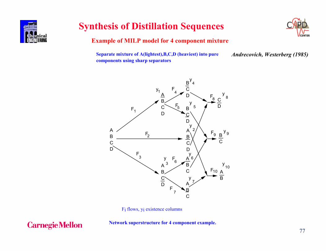
Example of MILP model for 4 component mixture

Separate mixture of A(lightest),B,C,D (heaviest) into pure components using sharp separators

A B C D

A B C D

A B C D

A B C D

B C D

B C D

A B C

A B C

C D

B C

A B

1

2

3

4

5

6

7

8

9

10F

F

FF

F

F

FF

F

F

1

3

8

9

10

4

5

2

6

7

y

y

y

y

y

y

y

y

y

y

Fi flows, yi existence columns Network superstructure for 4 component example.

Synthesis of Distillation Sequences

Andrecovich, Westerberg (1985)

78

Data for example problem a) Initial field FTOT = 1000 kgmol/hr Composition (mole fraction) A 0.15 B 0.3 C 0.35 D 0.2 b) Economic data and heat duty coefficients Investment cost Heat duty k Separator k, fixed, k, variable coefficients, Kk 1 A/BCD 145 0.42 0.028 2 AB/CD 52 0.12 0.042 3 ABC/D 76 0.25 0.054 4 A/BC 25 0.78 0.024 5 AB/C 44 0.11 0.039 6 B/CD 38 0.14 0.040 7 BC/D 66 0.21 0.047 8 A/B 112 0.39 0.022 9 B/C 37 0.08 0.036 10 C/D 58 0.19 0.044 Cost of utilities: Cooling water CC = 1.3 (103$hr/106kJyr) Steam CH = 34 (103$hr/106kJyr)

79

Split fractions in superstructure (using initial compositions)

1A = 0.15 6

A = 0.188

1BCD = 0.85 6

BC = 0.812

2A B = 0.45 7

A B = 0.5625

2CD = 0.55 7

C = 0.44

3A BC = 0.8 8

C = 0.636

3D = 0.2 8

D = 0.364

4B = 0.353 9

B = 0.462

4CD = 0.647 9

C = 0.538

5BC = 0.765 1 0

A = 0.333

5D = 0.235 1 0

B = 0.667

Assume perfect recoveries

80

MILP model

Initial node in network F1 + F2 + F3 = 1000 (1) For the remaining nodes in the network, mass balances for each intermediate product. Based on the recovery fractions, the mass balance for each intermediate product is as follows:

a) Intermediate (BCD) which is produced in column 1, and directedto columns 4 and 5, F4 + F5 - 0.85 F1 = 0 (2) b) Intermediate (ABC) which is produced in column 3, and directedto columns 6 and 7, F6 + F7 -0.8 F3 = 0 (3) c) Intermediate (AB) which is produced in columns 2 and 7, anddirected to column 10, F10 - 0.45 F2 - 0.563 F7 = 0 (4) d) Intermediate (BC) which is produced in columns 5 and 6, anddirected to column 9, F9 - 0.765 F5 - 0.812 F6 = 0 (5) e) Intermediate (CD) which is produced in columns 2 and 4, anddirected to column 8, F8 - 0.55 F2 - 0.647 F4 = 0 (6)

81

Relating flows to the binary variables y: Fk - 1000 yk ¡ Ü 0 , Fk ¡ Ý 0 , yk = 0,1 , k = 1,...10 (7) Heat duties of condensers and reboliers, continuous variables Qk , k = 1, ...10, Qk = Kk Fk , k = 1,...10 (8) where the parameters Kk are given in Table. Objective function, minimization of the sum of the costs in the 10columns.

min C = (ky k + kFk) + (34 + 1.3) Σk=1

10QkΣ

k=1

10

cost coefficients k , k , are given in Table.

0

Uyk

82

Optimal separation sequence

A B C D C

D

A BA

B C D

1000

450

550$3,308,000/yr

Second best solution. Make y2 = y8 = y10 = 1 infeasible y2 + y8 + y10 ? 2 Second best sequence

A B C D

B C D

C D

A B C D

1000850 550 $3,927,000/yr

83

Input

FeedEthane C2H6

Propane C3H8Butane C4H10

Naphtha C8~C12

RXN System

PyrolysisFurnaces

Components

MixtureHydrogen H2Fuel gas CH4

Acetylene C2H2Ethylene C2H4Ethane C2H6MAPD C3H4

Propylene C3H6Propane C3H8

C4 MixtureC5 Mixture

C6+ Mixture

Separation

SeparationTasks

RecycleEthane C2H6Propane C3H8

Output

Hydrogen H2

Fuel gas CH4

C5 Mixture

Ethylene C2H4

Propylene C3H6

C4 Mixture

C6+ Mixture

Olefin Separation System (BP)

Goal: Synthesize optimal separation system(Lee, Foral, Logsdon, Grossmann, 2003)

84

Process Superstructure

A/BCDEFGH

ABCDEFGH

STATES TASKS

AB/CDEFGH

ABCD/CDEFGH

ABCDEF/CDEFGH

ABCDEF/EFGH

ABCD/EFGH

ABCDEF/GH

ABCDEFG/H

ABCDEFG

BCDEFGH

NON-SHARP

A/BCDEFG

AB/CDEFG

ABCD/CDEFG

ABCDEF/CDEFG

ABCDEF/EFG

ABCD/EFG

ABCDEF/G

B/CDEFGH

BCD/EFGH

BCD/CDEFGH

BCDEF/CDEFGH

BCDEF/EFGH

BCDEF/GH

BCDEFG/H

ABCDEF

BCDEFG

CDEFGH

A/BCDEF

AB/CDEF

ABCD/CDEF

ABCD/EF

BCDEF/G

B/CDEFG

BCD/CDEFG

BCDEF/CDEFG

BCDEF/EFG

BCD/EFG

CDEFG/H

CD/EFGH

CDEF/EFGH

CDEF/GH

BCDEF

CDEFG

ABCD

AB

BCD

EFG

CDEF

EFGH

GH

EF

CD

A

B

C

D

F

E

G

H

CD/EFG

CDEF/EFG

CDEF/G

B/CDEF

BCD/CDEF

BCD/EF

A/BCD

AB/CD

CD/EF

EF/GH

EFG/H

B/CD

EF/GG/H

E/F

C/D

A/B

H2

CH4C2H4

C3H6C2H6

C3H8C4

C525 states53 separation task

Feed

85

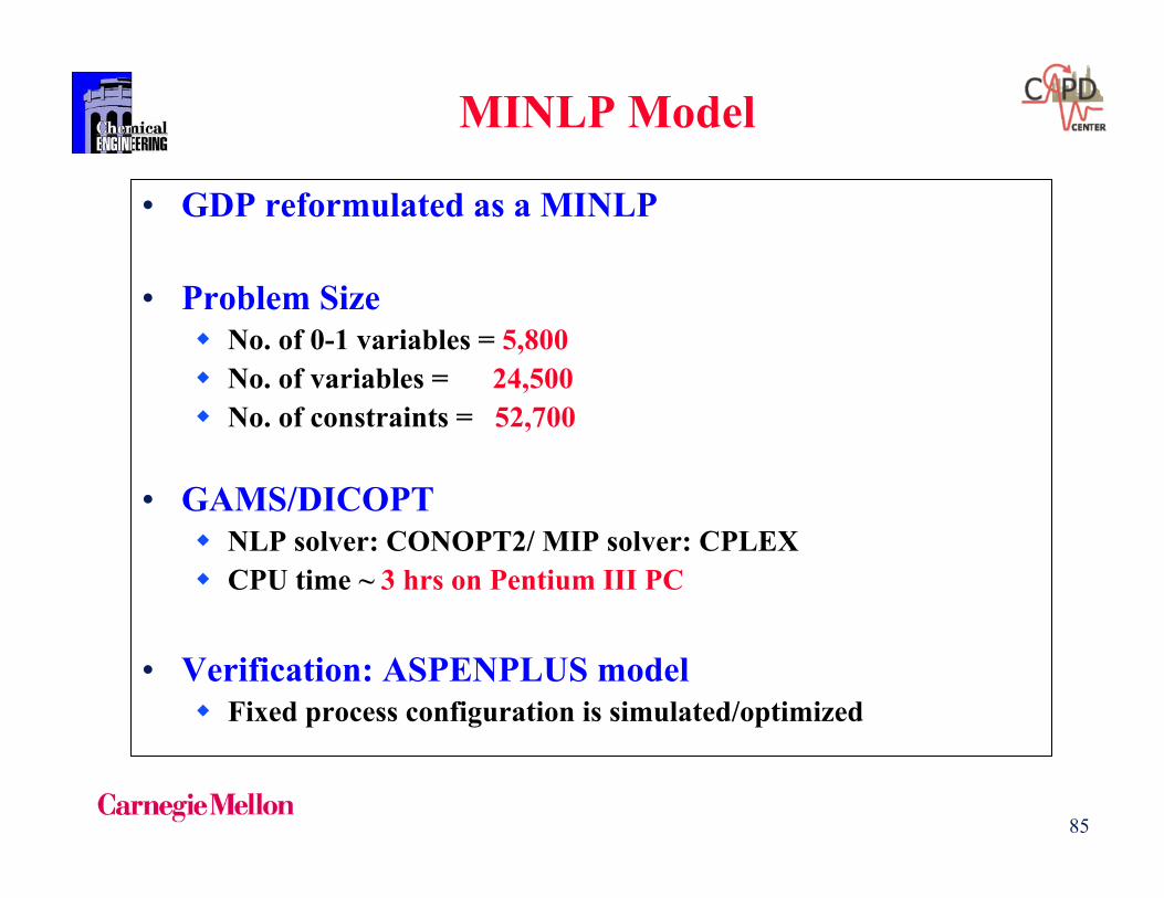
MINLP Model

• GDP reformulated as a MINLP

• Problem Size No. of 0-1 variables = 5,800 No. of variables = 24,500 No. of constraints = 52,700

• GAMS/DICOPT NLP solver: CONOPT2/ MIP solver: CPLEX CPU time ~ 3 hrs on Pentium III PC

• Verification: ASPENPLUS model Fixed process configuration is simulated/optimized

8686

Total cost: 110.82 MM$/yr

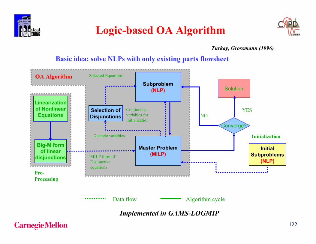
ABCDEFGH

AB

CDEFGH

EF

CD

B

A

D

C

E

F

H

G

A/B

CH4

C2H4

C3H6

C2H6

C3H8

C4

C5

H2

EFGH

Cold Box

Deethanizer

Dephlegmator

100F480Psig

83F160Psig

-141F900Psig

-41F160Psig

84F190Psig

169F160Psig

DE

EF

CD

123F140Psig

99F140Psig

GHGH

Depropanizer

C3Splitter

226F160Psig

compressor

heater

cooler

valve

480Psig

74F170Psig

72F140Psig

480Psig-31F140Psig

-51F140Psig

214F170Psig

109F140Psig

FG

Debutanizer

236F140Psig

238F140Psig

AB

CD

900Psig

Chemical Absorber

410 Mkwh/yr

valve

compressor

pump

pump

MINLP optimal solution

Dephlegmator first process7 separation units

1 dephlegmator1 absorber4 distillation columns1 cold box1 heat exchange

20M$/yr cost saving

8787

Optimal Feedtray Location

Sargent & Gaminibandara (1976)

NLP VMP: Variable-Metric Projection

ifNLP Formulation

Min costst MESH eqtns

FfLoci

i

8888

1

.

.

L1 V2

L2 V3

L3 V4

LN-1

1

2

3

N

N-1

N-2

VN

VN-1LN-

2

VN-2LN-

3

B

D1

.

.

L1 V2

L2 V3

L3 V4

LN-1

1

2

3

N

N-1

N-2

VN

VN-1LN-

2

VN-2LN-

3

B

D

LocizLocizFf

Ff

z

i

ii

Locii

Locii

1,00-

1if

Optimal Feedtray Location (Cont)

MINLP FormulationMin cost

st MESH eqtns

Viswanathan & Grossmann (1990)

MINLP DICOPT: AP-Outer Approximation-ER

F

Remark: MINLP solves as relaxed NLP!

Feed tray composition tends to match composition of feed

iz

8989

Optimization of Number of Trays

Discrete variables: Number of trays, feed tray location.Continuous variables: reflux ratio, heat loads, exchanger areas, column diameter.

No liquid on tray

No vapor on tray

Existing trays

Vapor Flow

Liquid Flow

Viswanathan & Grossmann (1993)

Zero flows- Discontinuities appear, convergence difficulties.Redundant equations are solved- Increases CPU time.

Non-existing tray

Non-existing tray

1=mzr

1=nzb

1,0=izb

MINLP => Numbertrays

1,0=izr

90

Optimal Design Columns with Multiple Feeds

60

59

F 2

F1

ri

1

(0.15, 0.85)

F 3

(0.5, 0.5)

(0.85, 0.15)

2

Separation Methanol - Water with 3 Feeds

MINLP modelVirial/UNIQUAC

115 0-1 binary variables

1683 continuous variables

1919 constraints

700,000 alternatives!

Air Products & Chemicals

Solved with DICOPT on a HP 9000/730 (5 major iterations, 45 min)

Optimal solution

Number of trays = 53

Feed location: Feed 1 Tray 4Feed 2 Tray 6Feed 3 Tray 12

Viswanthan & Grossmann (1993)

9191

Disjunctive Programming Model

Permanent trays:Feed, reboiler, condenser Conditional trays:Intermediate trays mightbe selected or not.

Conditional trays

Permanent trays

Trays not allowed to “disappear” from column:

VLE mass transfer if selected.No VLE, trivial mass/energy balance if not selected

-OR-VLE NOT VLE(tray bypass)

Disjunction

Yeomans & Grossmann (2000)

9292

Condenser Tray(permanent)

Rectification Trays(conditional)

Feed Tray(permanent)

Stripping Trays(conditional)

Reboiler Tray(permanent)Heavy Product

Feed

LightProduct

-OR-

-OR-

-OR-

-OR-

Vapor Flow

Liquid Flow

Equilibrium Stage

Non-equilibrium Stage

Single Column GDP Model

•Permanent and conditional trays:MESH equations for condenser,

reboiler and feed traysMass & energy balances for

rectification and stripping trays.

•Conditional trays only:Apply VLE constraints (Yn=True)

or not (Yn=False)Use disjunctions as modeling tool.

9393

Example GDP

GDP FormulationMixture: Methanol/Ethanol/water

Feed Flow= 10 mol/sec

Feed composition= 0.2/0.2/0.6

P = 1.01 bar

Product Specification: products composition reversible model

Upper bound No. Trays: 60

Ideal/Wilson models

Methanol/ethanol/water - GDP: fixed tray location Preprocessing Phase: NLP tray-by-tray Models

Continuous Variables 1597 Constraints 1544 Total CPU time (s) 1.12

Model Description

Continuous Variables 2933 Binary Variables 60 Constraints 2862 Nonlinear nonzero elements 5656 Number of iterations 10 NLP CPU time (s) 9.14 MILP CPU time (s) 16.97 Total CPU time (s) 401

Optimal Solution Total number of trays 41 Feed tray 20 Column diameter (m) 0.51 Condenser duty (KJ/s) 387.4 Reboiler duty (KJ/s) 386.5 Objective value ($/yr) 117,600

GAMS PIII, 667 MHz. with 256 MB of RAM.

CONOPT2 NLP subproblems/ CPLEX MILP subproblems.

Used Logic-based OA

94

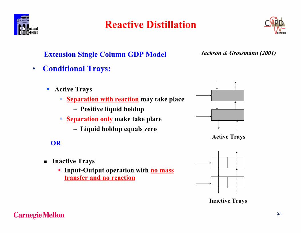
Reactive Distillation

• Conditional Trays:

Active Trays Separation with reaction may take place

– Positive liquid holdup Separation only make take place

– Liquid holdup equals zeroActive Trays

Inactive Trays

Inactive Trays Input-Output operation with no mass

transfer and no reaction

Extension Single Column GDP Model Jackson & Grossmann (2001)

OR

95

Example: Metathesis of Pentene

• Annualized Cost: $1.167x106 per year• Design/Operating Parameters:

21 Trays; 5 Feeds Column Diameter = 3.8ft Column Height = 107ft Boilup = 0.374 Reflux = 0.811 Reboiler Duty = 153 kW Condenser Duty = 984 kW

• Reaction Zone: Trays 1 – 18 Total Liquid Holdup = 752 ft3

90% Conversion of Pentene

11.1 C5H10

8.0 C5H10

69.5 C5H10

12.0 C5H10

19.5 C5H10

2.8 C5H10

53.7 C4H8

0.004 C6H12

9.3 C5H10

0.25 C4H8

53.9 C6H12

14

65

11

7

126841052 HCHCHC Conversion of 2-cis-pentene into 2-cis-butene and 3-cis-hexene:

GDP Model: 25 discrete variables731 continuous variables730 constraints

96

Superstructure Representation Suitable for zeotropic and azeotropic mixtures General and automatically generated Includes thermodynamic information Embeds many possible alternative designs

Synthesis of complex distillation systems

Mariana Barttfeld, Pio Aguirre/INGAR

Solution Procedure–Decomposition algorithm (decision levels)

•First level: selection of sections •Second level: selection of trays in existent sections

–Initialization phase: reversible sequence approximation –Robust and effective solutions

Superstructure Formulation GDP formulation

97

ABCD

ABCD

ABCD

A | BCD

AB | CD

ABC | D

ABCD

BCD

ABC

BCD

ABC

BCD

ABC

B | CD

BC | D

A | BC

AB | C

CD

CD

BC

BC

AB

AB

AB

BC

CD C | D

B | C

A | B

C

D

B

C

A

B

B

D

A

C

A

D

Pure Product State

Intermediate Product State

Initial State

Mixer / Splitter

Separation Task

Sharp separation 4 components

State Task NetworkAndrecovich, Westerberg (1985)

98

ABCD

A | BCD -or-

AB | CD -or-

ABC | D

B | CD -or-

BC | D -or-

A | BC -or-

AB | C -or-

C | D

A | B -or- B | C -or- C | D

S3

S1

S2

S4

S5

S6

S7

S8

S9

S10

S11

S12

S13

S14

S15

S16

S17

S18

TASKS

S16- AB, BC, CD S17- A, B, C S18- B, C, D

S1- A, AB, ABC S2- BCD, CD, D S3- ABC S4- BCD, CD S5- AB

S6- CD S7- BCD, CD, ABC S8- A S9- D S10- CD, D, BC, C

S11- B, BC, A, AB, C S12- CD, BC S13- BC, AB S14- C, D S15- A, B C

STATE DEFINITION

Sharp separation 4 components

State Equipment Network (SEN)Kravanja et al (1995)

9999

ABCD

ABC

BCD

AB

BC

CD

A

B

C

D

States

Tasks

STN Representation(4 Component Zeotropic Mixture)

B C

C D

A B

A B C

B C D

A

A B C D

B

C

D

Sargent-Gaminibandara Superstructure(4 Component Zeotropic Mixture)

Superstructure for Complex Distillation Rigorous Model

Generated with the State-Task-Network (STN) (Sargent, 1998)

100100

B C

C D

A B

A B C

B C D

A

A B C D

B C

B

C

B

C

D

States

Tasks

ABCD

BCD

ABC

AB

BC

CD

A

B

C

D

BC

RDSM-based STN Representation

(4 Component Zeotropic Mixture)

Avoid mixing intermediates

Based on the Reversible Distillation Sequence Model (RDSM) (Fonyo, 1974)Motivated by thermodynamic initialization scheme

Automatically generated with the State-Task-Representation (STN)Contains 2NC-1-1 columns and NC-1 level

Superstructure Zeotropic MixturesBartfeld, Aguirre, Grossmann (2004)

101101

ABC

ABC

BC

AB

BC

A

B

B

Azeotrope

C

A

BC

F

ABC

BC

BC-Azeo

Product Azeotrope

Mass BalanceDistillation Boundary

ABC

BC

ABC

AB

BC

C

A

B

Azeo

B

Azeo

States

Tasks

RDSM-based STN Representation(4 Component Azeotropic Mixture)

RDSM-based STN cannot be defined a prioriComposition diagram neededAzeotrope recycled

Modification for Azeotropic Mixtures

102102

B C

A B C

B C D3

6

1

5

2

A

A B C D

B C

B

C

B

C

D

6

5B C

B C

C

A

A B C D

D

B

B C D3

6

5

B C

A B C

A

A B C DB C

C

D

B2

1

B C

C D

A B

A B C

B C D

A

A B C D

B C

B

CB

C

D

1

2

3

4

5

6

7

Mapping to Specific Designs

103103

section s+1

section s Selection of sections ConfigurationIf section selectedYs = TrueIf section not selected Ys = False

Discrete Decisions

Two hierarchical levels1. Selection sections2. Selection Trays

104104

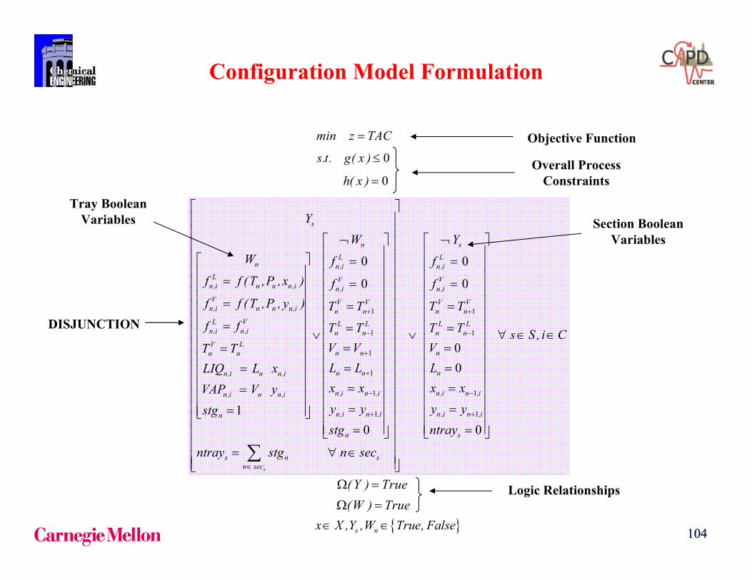
1

1

1

1

1

1

0

0

10

s

nL

n n,iL V

n,i n n n,i n ,iV V V

n,i n n n,i n nL V L L

n,i n ,i n nV L

n nn n

n nn,i n n,i

n ,i n ,in ,i n n,i

n ,i n ,in

n

YW

W ff f (T ,P ,x ) ff f (T ,P , y ) T Tf f T T

V VT TL LLIQ L xx xVAP V yy ystgstg

1

1

1

1

0

0

00

0

s

sL

n,i

Vn,i

V Vn nL L

n n

n

n

n,i n ,i

n ,i n ,i

s

s n sn sec

Y

f

f

T T

T TVLx xy yntray

ntray stg n sec

s S , i C

min z TAC

0s.t. g( x )

0h( x )

(Y ) True

(W ) True

s nx X ,Y ,W True, False

Objective Function

Overall Process Constraints

Logic Relationships

Section Boolean Variables

Tray Boolean Variables

DISJUNCTION

Configuration Model Formulation

105

Detailed Cost Functions

dep

CinvTAC CopT

Annual Cost

agua vaporagua con vap

Qc QhCop C CCp T H

Operating Cost

Cinv Ccol Ctray Creb Ccond 1 066 0 802. .

colCcol k nt Dcol htray

1 55.trayCtray k nt Dcol htray

0 65.rebCreb k Areb

0 65.condCcond k Acond

Investment Cost

Column Cost

Tray costs

Condenser Cost

Reboiler cost

nDcol Dtray

0 50 5 ..vapor

n d n i n,ii

T RDtray k V PM y

p

106

Solution Strategy

GDP Section

Problem

-Selection of Sections-MILP

Problem

-Selection of Trays-MILP

Problem

Reduced NLPProblem

-Initialization Phase-NLP

Problems

GDP Tray

Problem

Preprocessing

Phase

Algorithm Cycle

Fixed MaxNumber Trays

Fixed NumberSections

Aggregate NLPNLP fixed max number trays

107

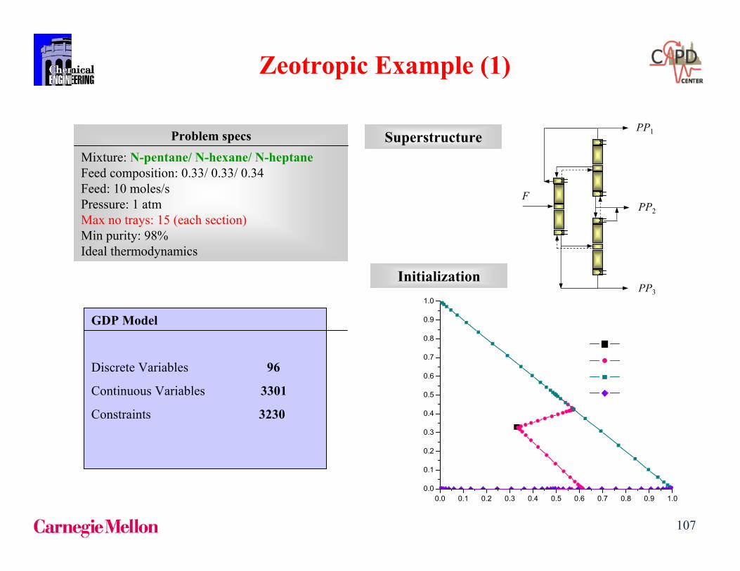
Problem specsMixture: N-pentane/ N-hexane/ N-heptaneFeed composition: 0.33/ 0.33/ 0.34Feed: 10 moles/sPressure: 1 atmMax no trays: 15 (each section)Min purity: 98%Ideal thermodynamics

SuperstructurePP1

PP2

F

PP3

0.0 0.1 0.2 0.3 0.4 0.5 0.6 0.7 0.8 0.9 1.00.0

0.1

0.2

0.3

0.4

0.5

0.6

0.7

0.8

0.9

1.0

Initialization

Zeotropic Example (1)

GDP Model

Discrete Variables 96

Continuous Variables 3301

Constraints 3230

108

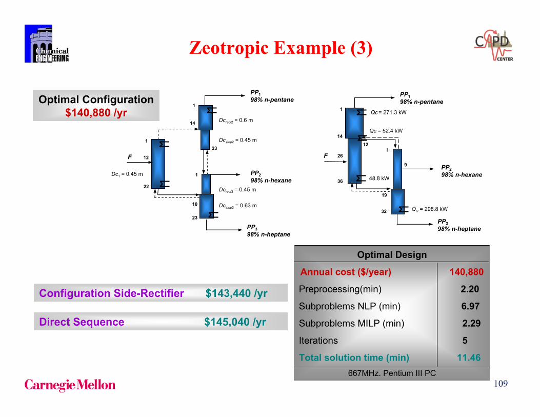
Optimal Configuration$140,880 /yr

Optimal Design

Annual cost ($/year) 140,880

Preprocessing(min) 2.20

Subproblems NLP (min) 6.97

Subproblems MILP (min) 2.29

Iterations 5

Total solution time (min) 11.46667MHz. Pentium III PC

0.0 0.1 0.2 0.3 0.4 0.5 0.6 0.7 0.8 0.9 1.00.0

0.1

0.2

0.3

0.4

0.5

0.6

0.7

0.8

0.9

1.0

Mol

e Fr

actio

nn-

pent

ane

Mole Fraction n-hexane

FeedCol 1 (tray 1 to 14)Col 1 (tray 15 to 34)Col 2 (tray 1 al 9)Col 2 (tray 10 al 32)

PP398% n-heptane

36

9

32

PP298% n-hexane

26

19

PP198% n-pentane

F

Qc = 52.4 kW

QH = 298.8 kW

48.8 kW

1

11 12

14

Qc = 271.3 kW

PP398% n-heptane

12

23

PP298% n-hexane

10

PP198% n-pentane

F

1

22

Dc1 = 0.45 m

Dcrect2 = 0.6 m

Dcstrip2 = 0.45 m

1

14

23

1

Dcstrip3 = 0.63 m

Dcrect3 = 0.45 m

Zeotropic Example (2)

All sections selected

109

Optimal Configuration$140,880 /yr

Optimal Design

Annual cost ($/year) 140,880

Preprocessing(min) 2.20

Subproblems NLP (min) 6.97

Subproblems MILP (min) 2.29

Iterations 5

Total solution time (min) 11.46667MHz. Pentium III PC

PP398% n-heptane

36

9

32

PP298% n-hexane

26

19

PP198% n-pentane

F

Qc = 52.4 kW

QH = 298.8 kW

48.8 kW

1

11 12

14

Qc = 271.3 kW

PP398% n-heptane

12

23

PP298% n-hexane

10

PP198% n-pentane

F

1

22

Dc1 = 0.45 m

Dcrect2 = 0.6 m

Dcstrip2 = 0.45 m

1

14

23

1

Dcstrip3 = 0.63 m

Dcrect3 = 0.45 m

Configuration Side-Rectifier $143,440 /yr

Direct Sequence $145,040 /yr

Zeotropic Example (3)

110110

Problem Specs

Mixture: Methanol/ Ethanol/ WaterFeed composition: 0.5/ 0.3/ 0.2Feed: 10 moles/sPressure: 1 atmMax no. trays: 20 (per section)Min purity: 95%Ideal/Wilson models

F

methanol

ehtanol

Azeotrope

Water

ethanol

Superstructure

Initialization

GDP Model

Discrete Variables 210

Continuous Variables 9025

Constraints 8996

Bartfeld, Aguirre, Grossmann (2004)

Azeotropic Example

111111

Product Specifications 95%Optimal Configuration $318,400 /yr

Optimal Solution

Annual Cost ($/year) 318,400

Preprocessing (min) 6.05

Subproblems NLP (min) 36.3

Subproblems MILP (min) 3.70

Iterations 3

Total Solution Time (min) 46.01667MHz. Pentium III PC

Profiles Optimal Configuration

F

PP6 = 1.292 mole/sec95% Water

PP1 = 5.158 mole/sec95% Methanol

PP4 = 0.836 mole/sec95% Ethanol

39

38

35

PP5 = 2.376 mole/secAzeotrope

622 kW

260 kW

200 kW

4 out of 10 sections deleted

Azeotropic Example

• STATES: Intensive and extensive physical and chemical properties of a stream.

* Quantitative (composition, temperature)* Qualitative (phase, components present)

• TASKS: Physical or chemical transformations between adjacent states (momentum, heat and mass transfer operations).

* Permanent- Valid throughout flowsheet.* Conditional- May not exist for a given flowsheet.

• EQUIPMENT: Physical device that executes a task (design equations and parameters)

* Permanent or Conditional.

Yeomans, Grossmann (2000)

Elements for Flowsheet Superstructures

State Task Network

• First step: State and Task Identification in process flowsheet.

1

2

3

4

5

6

7

9

11

10

12

13

T1

T2

T3

T4

T5 T7

T8

T9

STATES: 1- A Raw, V, Low P 2- A mixed, V, Low P 3- A mixed, V,Low P to T3 4- A mixed, V,Low P to T4 5- A,V, High P form T3 6- A, V, High P form T4 7- A, V,High P, to preheat 8- A,V High P, High T 9- A ,V to packed reactor 10- A+B, V to mixer T10 11- A, V , to PFR

15 T12

T13

12- A+B, V to mixer T10 13- A+B, V to cooler 14- A+B, L to flash. 15- A+B, Rich in A, V, from purge splitter 16- A,V, low P 17- A+B, L, to distillation 18- B, L, Final Product 19- A, V, High P 20- A+B, V to purge 21- A+B, V, waste product

TASKS: 1- Mix recirc A and raw A 2- Split feed mixture 3- Compress in single stage 4- Compress in two stages 5- Mix compressed streams and recycle. 6- Preheat for reaction 7- Split to reactors 8- React A->B in the vapor phase in PFR

9- React A->B in vapor phase with catalizer C in packed reactor 10- Mix reactor outlets, Vapor 11- Condense stream 12- Flash A+B: A+B vapor, B liquid 13- Distillate A+B: A liquid, B liquid 14- Compress col. vapor outlet 15- Purge vapor stream

8T6 T10

T11

14

19

18

17T14 16

20

21

T15

state 19

task 14

OTOE Assignment for STN

• Predetermined Equipment Assignment: One Task One Equipment

REACTOR 2:A-cat->B

COMPRESSOR 1

COMPRESSOR 2

FLASH

COLUMN

REACTOR 1:A-->B

PRE-HEATERCOOLER

FEED

PRODUCT

VTE Assignment for STN

• Assignment left over for optimization: Variable Task Equipment

13

T11

141

2

3

4

5

6

7

9

11

10

12

T1

T2

T3

T4

T5 T7

T8

T9

20

T12

T13

8T6 T10

T1419

18

1716

15

21

T15

State Equipment Network (SEN)

VTE:

Compress Recycle-or-Compress Feed

Equipment Tasks

Preheat feed to reactor-or-Cool reactor outlet-or-Vaporize recycle from distillation

React A-->B (liquid phase)-or-React A-cat->B in packedreactor (vapor phase)

1 stage 2 stage

state iequipment j

FEED

PRODUCT

GDP Model for State Task Network / OTOE

• Boolean Variable Yt:

* True- Task exists, task and equipment equations apply

* False- Equipment does not exist. A subset of variables is set to zero.

min cttT sxs

sS

s. t. gt(dj' ,zt ,xs ,xs' ) 0ct f (dj' ,zt )

j'Qt , t TP

sIt , s'Ot

Ytgt(dj' ,zt ,xs ,xs' ) 0

ct f (dj' ,zt )

j'Qt

sIt ,s'Ot

Ytdj' zt 0xs xs' 0

j'Qt

sIt ,s'Ot

tTC

(Y ) True

d D, z Z, x X Yt True, False

Conditional Task (TC)

PermanentTask (TP)

REACTOR 2:A-cat->B

COMPRESSOR 1

COMPRESSOR 2

FLASH

COLUMN

REACTOR 1:A-->B

PRE-HEATER COOLER

FEED

PRODUCT

GDP Model for SEN

• Boolean Uj for equipment existence.

• Boolean Variable Vjt:* True- Apply design

equations for task t.* False- Do not apply design

equations for task t.min cjt

tT

jE s xs

sS

s. t.

t Bj

Vjt

ptj(dj , zt , xs ,xs' ) 0c jt f (dj , zt )

j EP

tBj

Uj

V jt

ptj (d j , zt , xs , xs' ) 0ctj f (dj , zt )

Uj

zt dj 0xs xs' 0

jEC

(V ,U) True

d D, z Z, x X, Vjt True, False,Uj True, False

PermanentEquipment

(EP)

Conditional Equipment (EC)

Theoretical Properties

• Model comparison (STN vs. SEN):

* One Task - One Equipment assignments lead to simpler disjunctive models

* SEN is equivalent to STN / OTOE if each equipment is allowed to perform only one task, provided same tasks appear in both

* STN / VTE leads to different model than SEN. The same problem and same assignment (VTE) generate physically different superstructures

* No model is inherently tighter than the other.

120

Flowsheet Synthesis: MINLP Approach (OTOE)HDA process: 13 0-1 variables, 723 variables, 719 constraints DICOPT: 7.5 secs

Methane Purge

Hydrogen Feed

Toluene Feed

Methane Purge

Methane Purge

Benzene Product

Diphenyl Byproduct

Toluene

Membrane #1

Furnace

Adiabatic Reactor

Isothermal Reactor

Quench Membrane #2Flash

#1

Flash #2

Flash #3

Benzene Column

Toluene Column

Stabilizing Column

Absorber

Hydrogen Recycle

Toluene Recycle

LEGEND FOR INTERCONNECTION NODES

Single choice stream splitter

Multiple choice stream splitter

Single choice stream mixer

Multiple choice stream mixer

192 embedded flowsheets

13 bin. var. 672 cont. var. 678 constr.

121

Hydrogen Feed

Toluene Feed

Methane Purge

Methane Purge

Benzene Product

Diphenyl Byproduct

Furnace

Adiabatic Reactor

QuenchFlash

#1

Benzene Column

Toluene Column

Stabilizing Column

Hydrogen Recycle

Toluene Recycle

PROFIT = 4.814 M$/yr

Potential Problems:1. Zero flows2. Large dimensionality

--- DICOPT: Log File:Major Major Objective CPUtime Itera- Evaluation SolverStep Iter Function (Sec) tions ErrorsNLP 1 5750.63780 1.81 2490 0 snoptMIP 1 3312.01424 0.33 443 0 cplexNLP 2 4057.62731< 1.59 2038 0 snoptMIP 2 2227.55081 0.33 713 0 cplexNLP 3 4047.47058 3.50 2222 0 snopt

--- DICOPT: Terminating...--- DICOPT: Stopped on NLP worsening

Profit= 4.057M$/yr

122122

Logic-based OA Algorithm

Master Problem(MILP)

Subproblem(NLP)

Selection ofDisjunctions

Converge?

Solution

InitialSubproblems

(NLP)

Linearizationof NonlinearEquations

Big-M formof linear

disjunctions

Pre-Processing

MILP form ofDisjunctiveequations

Continuousvariables forInitialization

Discrete variables

Selected Equations

YESNO

Initialization

OA Algorithm

Data flow Algorithm cycle

Implemented in GAMS-LOGMIP

Turkay, Grossmann (1996)

Basic idea: solve NLPs with only existing parts flowsheet

123

Pby

1

2

3

4 5 6

7 8

9

10

1112 13

14

15

16

171819

A + B C

90% pure C

Š1,000 ton/day

Feed 1 (cheap)

Feed 2 (exp.)

high conv, high cost

low conv, low costP, conv ?

Example Superstructure Process Flowsheet

To apply Logic-based OA we require NLP subproblems to cover all units

Remark. Fewest number subproblems: set covering problem

(OTOE)

124

Pby

1

4 5 6

7 8

10

1112 13

14

15

171819

A + B C

90% pure C

1,000 ton/day

Feed 1 (cheap)

low conv, low cost

P=15MPa conv=27.6% /pass

Subproblem 1 (NLP): $859,000/yr

Pby

2

3

7 8

9

1112 13

14

15

16

A + B C

90% pure C

1,000 ton/dayFeed 2 (exp.)

high conv, high cost

P=11MPa conv=33.2% /pass

Subproblem 2 (NLP): $1,575,000/yr

All units covered => MILP Master 1: $1,868,000/yr

125

Pby

2 4 5 6

7 8

9

1112 13

14

15

16

A + B C

90% pure C

1,000 ton/dayFeed 2 (exp.)

high conv, high cost

P=13.8MPa conv=30.1% /pass

Subproblem 3 (NLP): $1,794,000/yr

MILP Master 2: $1,741,000/yr (with integer cut)

Since $1,741,000/yr < $1,794,000/yr STOP!

126126

Superstructure Vinyl Chloride Monomer (Turkay & Grossmann, 1997)

Oxygen

Air

Ethylene

Chlorine

Vinyl Chloride

Hydrogen Chloride

Ethylene Dichloride

Ethylene Dichloride

Water

Flash

Direct Chlorination

Oxychlorination

Low P

High P

Purge

Hydrogen Chloride

Process Flowsheet Synthesis

Major options:Direct Chlorination vs. OxychlorinationAir vs. OxygenPressure PyrolisisSeparation sequenceOptimization with discontinuous cost models:

- Multiple size regions- Pressure, temperature factors

Cost

Size

127

Optimal Solution (CPU-time: 3.8min)

Oxygen

Ethylene

Chlorine

Vinyl Chloride

Hydrogen Chloride

Ethylene Dichloride

Water

Flash

Direct Chlorination

Oxychlorination

High P

Purge

Profit=$75.3 million/yr

Item Flowsheet 1 Flowsheet 2 Master Pr. 1 Flowsheet 3 Master Pr. 2

Binary var. 162 168 259 168 259 Continuous var. 879 883 1715 883 1822

Constraints 699 703 1750 703 1858 Profit ($M/yr) 27.678 75.283 82.763 71.809 65.262

Major Iterations 3 3 N/A 3 N/A CPU time (sec) 88.00 64.99 8.24 53.76 13.21

128

Carnegie Mellon

US Energy Sources

Biomass emerging as important renewable

129

Carnegie Mellon

Process Design Challenges in BioethanolEnergy consumption corn-based process level:

Water consumption corn based - process level:

Author (year) Energy consumption (Btu/gal)

Pimentel (2001) 75,118

Keeney and DeLuca(1992)

48,470

Wang et al. (1999) 40,850

Shapouri et al. (2002) 51,779

Wang et al (2007) 38,323

Author (year) Water consumption( gal/gal ethanol)

Gallager (2005) First plants

11

Philips (1998) 5.8

MATP (2008) Old plants in 2006

4.6

MATP (2008) New plants

3.4

130

Carnegie Mellon

Proposed Design Strategyfor Energy and Water Optimization

Energy optimizationIssue: fermentation reactions at modest temperatures

Multieffect distillation followed by heat integration process streams

=> No source of heat at high temperature as in petrochemicals

Water optimizationIssue: cost contribution is currently still very small

(freshwater contribution < 0. 1%)

=> Total cost optimization is unlikely to promote water conservation

Optimal process water networks for minimum energy consumption

131

Carnegie Mellon

Energy Optimization of Corn-based BioethanolPeschel, Martin, Karuppiah, Grossmann, Zullo, Martinson (2007)

60 M gallon /yr plant

Equipment cost = M$ 18.4 Steam cost = M$ 21/yr Prod. cost = 1.50 $/gal

132132

Required operations

Ethanol purificationSolids drying

Molecular Sieves vs Corn GritsMechanical press before/after Beer column

Superstructure of a Bio-ethanol Plant

133133

Alternatives for Energy Reduction

HeatHeat IntegrationIntegration processprocess streamsstreams::

MultieffectMultieffect columnscolumns::

Low Pressurecolumn

High Pressurecolumn

GDP model comprises mass, energy balances, design equations (short cut)2,922 variables (2 Boolean) 2,231 constraints

134134

60 M gallon /yr plant

Ethanol losses : 0.5%

Optimized Structure

Equipment cost = M$ 20.7 Steam cost = M$ 7.1/yr (-66%) Prod. cost = 1.28 $/gal

HeatHeat IntegrationIntegration andandMultieffectMultieffect ColumnsColumns

Reduction from $1.50/gal (base case) to $1.28/gal !

135135

Energy Profiles in Multieffect ColumnsBeer Column

Rectification Column

Single columnSingle column

Single columnSingle column

Triple effect columnTriple effect column

Double effect columnDouble effect column

136

Carnegie Mellon

Remarks

Current ethanol from corn and sugar cane and biodiesel from vegetable oilscompete with the food chain.

U.S. Government policies support the production of lignocellulosic basedbiofuels and the reuse of wastes and new sources (algae)

137

Carnegie Mellon

Cellulosic Switchgrass and Microalgae highest yield (gal/acre)

Note: Switchgrass almost 3 times yield than Corn

138

Carnegie Mellon

Challenge:

Many alternative flowsheets

b) Hydrolysis Process (fermentation)

WastewaterPower-Heat

BiomassPretreatment

Cellulosic Hydrolysis

SugarFermentation

EthanolRecovery

Electricity

Feed Ethanol

a) Thermochemical Process (gasification)

Power-HeatGasification Gas clean-up

Fermentationor Catalytic

EthanolRecovery

Electricity

Feed Ethanol

Lignocellulosic Bioethanol

139

Carnegie Mellon

Superstructure Thermochemical Bioethanol

Process Design Alternatives:

GasificationIndirect Low pressureDirect high Pressure

Reforming.Steam reformingPartial oxidation

CO/H2 adjustmentWGSRBypassMembrane/PSA

Sour gases removal:MEAPSAMembrane

SynthesisFermentation

RectificationAdsorption Corn gritsMolecular sievesPervaporation

CatalyticDirect SequenceIndirect sequence

Ethanol via gasification

-Martin, M. Grossmann, I. E (2010) Aiche J. Submitted

Gasification Reforming Clean upCO/H2 Adj. Sour gases removal

Fermentation

Catalysis

Martin, Grossmann (2010)

140

Carnegie Mellon

Superstructure

Gasifier 1 Gasifier 2

Partialoxidation

Steam reforming

Partialoxidation

Steam reforming

Catalysis Fermentation Catalysis Fermentation Catalysis Fermentation Catalysis Fermentation

Problem

Subproblem

(A) (B) (C) (D) (E) (F) (G) (H)

Solution Strategy Energy Optimization

Decomposition of GDP in 8 subproblemsDecision levels: Gasifier

Removal HCsReaction of Syn Gas

Heat integration and economic evaluation

141

Carnegie Mellon

Ethanol: $0.81 /gal (no H2 credits)$ 0.42/gal (H2 credits)

Optimal Design of Lignocellulosic Ethanol Plant

Low cost is due to H2 productionEach NLP subproblem: 7000 eqs., 8000 var~25 min to solve

$67.5 Million/yr

1,996 Btu/gal (< 1/10th of corn!)

142

Carnegie Mellon

Superstructure Biothanol via Hydrolysis

Dilute acid

AFEX

Hydrolysis and Fermentation

Rectification

Adsorption

Molecular sieves

Pervaporation

143

Carnegie Mellon

Optimal Flowsheet

$48 Million/yr vs. $67.5 Million/yr (gasification)

144

Carnegie Mellon

Orange: Energy consumed after superstrucure optimization with heat integration. Red: Energy consumed after the contribution of lignin Blue: Cooling water requirements after heat integration

Impact of Lignin

145145145

Bioethanol Plant: no water managementAhmetovic, Martin, Grossmann (2009)

146

Carnegie Mellon

Freshwater

Dist. Colums.

Fermentor

Washing

Discharge

Solids removal

Organics removal

Optimal Water Network: Corn Ethanol

TDS removal

-Ahmetović , E., Martin, M. Grossmann, (2009) I&ECR. 2010, 49, 7972–7982

Gal. Water/Gal. Ethanol = 1.5

1.5 vs 3.4

Reduction freshwaterfrom 9.07 to 1.17!

147

Carnegie Mellon

Industrial Average

Industrial Goal

a- Superstrucure opt.b- Supers. + HENc- Supers. + HEN + Mult. d- Supers. + HEN + Mult (opt. reflux ratio)

Evolution of Water Consumption

Synergy with Heat Recovery

148

Carnegie Mellon -Martin, M. , Ahmetović, E., Grossmann, I. E (2010) I&ECR ASAP

Cellulosic Bioethanol via Gasification

Freshwater

Wastewater

Gasifier

Washing Solids removal

Organics removal

Optimal Water Network: Lignocellulosic Ethanol

Gal. Water/Gal. Ethanol = 4.2

149

Carnegie Mellon

Optimal Water Network: Lignocellulosic Ethanol

Cellulosic Bioethanol via HydrolisisGal. Water/Gal. Ethanol = 1.7

150

Carnegie Mellon

Table Summary of results [6-10]

A C BD F E

[6] Martín, M., Grossmann, I.E. (2011) AIChE J. DOI: 10.1002/aic.12544[7] Martín, M., Grossmann, I.E. Energy optimization of Hydrogen production from biomass. Rev. Submited to Comp. Chem. Eng.[8] Martín, M., Grossmann, I.E. Energy optimization of lignocellulosic bioethanol production via Hydrolysis to be submitted AIChE J.[9] Martín, M., Grossmann, I.E. Process optimization of FT‐ Diesel production from biomass. To be submitted[10] Martín, M., Grossmann, I.E. Process optimization bioDiesel production from cooking oil and Algae. To be submitted

(*) kg instead of gal

151

Sequential Modular Simulators Equation Based Simulators

Equipment libraries data bases Component property data basesProperties estimation

Numerical methods specifically developed for each process unit.Including Flash calculations in all the streams.

There is no difference between equations. The complete system is represented and solved by a set of equations without taking into account where they come from.

Rigid Input-output structure: Lack of flexibility. Convergence of recycles based on fixed point or quasi-Newton (Broyden) methods.

Initialization methods specifically design for each unit.

In general, no specific initialization methods.

Very flexible. Almost any specification possible. Quadratic Convergence(Newton based methods for solving equations).

Very robust and reliable. Faster, and more flexible but less robust and reliable

Disjunctive Representation with Implicit ModelsCaballero, Odjo, Grossmann (2007)

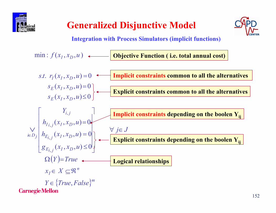
152

),,(:min uxxf DI

Jj

uxxg

uxxh

uxxh

Y

DIjiE

DIjiE

DIjiI

ji

jDi

0),,(

0),,(

0),,(

,

,

,

,

m

nI

FalseTrueY

Xx

TrueY

,

0),,(0),,(0),,(..

uxxsuxxsuxxrts

DIE

DIE

DII

Generalized Disjunctive Model

Objective Function ( i.e. total annual cost)

Implicit constraints common to all the alternatives

Implicit constraints depending on the boolen Yij

Logical relationships

Explicit constraints common to all the alternatives

Explicit constraints depending on the boolen Yij

Integration with Process Simulators (implicit functions)

153

),,(:min uxxf DI

Jj

uxxguxxhuxxh

Y

DIE

DIE

DII

ji

jDi

0),,(0),,(0),,(

,

m

nI

FalseTrueY

Xx

TrueY

,

0),,(0),,(0),,(..

uxxsuxxsuxxrts

DIE

DIE

DII xI Independent variables: Specifications or degrees of freedom in the modular process simulator (or any other third party program). The user has a complete control over these variables.

xD Dependent variables. They can only be read. Their value depend on the xI variables.

u variables that must be fixed. The user has only an indirect control of these variables (i.e. trays in a column).

Disjunctive Representation

154

Algorithms

Regular and Disjunctive Branch and Bound (Gupta & Ravindran,1985; Lee & Grossmann,2000)

Solve series of NLP problems in a tree search (no Master needed)

Outer Approximation –MINLP reformulation- (Duran and Grossmann,)Logic Based Outer Approximation (Turkay & Grossmann, 1996)Modeling and Decomposition (Kocis & Grossmann, 1989)

LP-NLP Based Branch and Bound (Quesada and Grossmann, 1992)Logic LP-NLP Based Branch and Bound

-Iterate between NLPs and Master (MILP) problems.-In Outer Approximation the Master is solved to optimality in each major iteration.-In LP-NLP based branch and bound the an NLP problem is solved when an Integer solution is found in the tree search of Master problems, all open nodes in the Master are then updated.

155

Solution Algorithms

Step 1. In the process simulator:

If the topology is fixed:

Select the independent variables (specifications). Chose a set of variables that makes that the simulation converges easily. -Difficult constraints or difficult specifications should be donethrough external constraints-.

If the topology is variable: (not all the units necessarily exist in a feasible flowsheet)

It is necessary to study of each unit in order to prevent unexpected behavior, i.e. Lack of convergence due to zero flows. If possible select the variables that minimizes (or avoid) thoseproblems.

In some situations it would be necessary especial algorithms . For process synthesis a good option are the “logic based algorithms”(Turkay and Grossmann, 1996), (Kocis and Grossmann, 1989)

156

Step 2. a. In the disjunctions there are no implicit equations:

Reformulate to MINLP using Big M or Convex Hull.

b. In the disjunctions there are implicit equations, but they do not affect the topologyReformulate to MINLP using a Big M reformulation.

c. In the disjunctions there are implicit equations that modify the topologySolve each of the fixed topology NLP subproblems, or the ‘main’ subproblem

and perform sub-lagrangian optimizations of the other units. (Logic Based Algorithms)

Solve the following NLP (r-MINLP).

0),,(0),,(0),,(..

),,(:min

uxxsuxxruxxrts

uxxf

DIE

DIE

DII

DIIx

0),,,(

0),,,(

,,*

,,*

jiDIjiE

jiDIjiE

yuxxg

yuxxh

100

ybAy

Implicit equations (i.e. process simulator)

Big M, convex hull reformulation or fixed topology sub-problem

Algebraic representation of logical equations, in terms of binary variables

157

Step 3. Generate (if necessary) the following Master MILP Problem

)(min 4321,,ssssT

sIx

)(]),(,[]),(,[ kII

kID

kIIx

kID

kI xxuxxxfuxxxf

2

11

)(]),(,[]),(,[

)(]),(,[

sxxuxxxsuxxxs

sxxuxxxrkIIIDIEIxIDIE

kII

kID

kIEIx

T

4,,

,*

,*

3,,

,*

2

],),(,[],),(,[

],),(,[

syyxxyuxxxgyuxxxg

syyxxyuxxxh

kjiji

kIIk

jikID

kIEIx

kji

kID

kIE

kjiji

kIIk

jikID

kIEIx

T

my

bAy

1,0

0

Notes:MILP only depends on xI and slacks.

xD is a function of xI. The linearization is done using the chain rule through the flowsheet or the implicit equations.

),( uxx IID

I

D

DIIx xd

xdxf

xff

k = 1, 2….K

158

Practical Implementation

Flowsheet simulated and converged in HYSYS.Plant 3.2

All algorithms BB, OA, LP-NLP_BB were implemented in MATLAB 7.1.

All the steps: generation and solving Masters and NLPs problems are controlled from MATLAB.

Auxiliary NLP and MILP solvers external to process simulator:MATLAB-TOMLAB (SNOPT 7, CONOPT 3, CPLEX 10)

Communication between MATLAB and HYSYS through ActiveX (Windows COM)

All other implicit equations (all but those in the process simulator) were developed as functions in MATLAB.

159

MATLAB HYSYS

Set up HYSYS Flowsheet.Start from a converged flowsheet

(external constraints can be violated)

Set up communicationMATLAB – HYSYS

(Windows COM)

Choose Algorithm (BB, OA, LP-NLP_BB)Set up initial NLP(s): (MINLP reformulations…)

Solve NLPsMATLAB-TOMLAB

(conopt3, snopt7)

xI variables

xD variables

HYSYS or other third party program or moduleDerivatives

Generate Master MILP

Solve Master ProblemMATLAB-TOMLAB

(CPLEX )

160

Example 1 Three heat exchangers network (Adapted from Turkay and Grossmann, 1996)

HYSYS Flowsheet

226.9 ºC

266.9 ºC

76.85 ºC

66.85 ºC

CostInvestmentutilitiesCost :min

5025

46500600

2510

150001500

101

30002750 6.0

3,

6.0

2,

6.0

1,

j

jj

j

j

jj

j

j

jj

j

A

ACI

Y

A

ACI

Y

A

ACI

Y

Some Data

Stream Tin (K) Tout (K) Cost ($/kW-year)Hot 500 340Cold 350 560Cooling W 323 363 20Heating V 557 557 80

Heat Exchanger U (kW/ m2 K)E-101 1.5E-102 0.5E-103 1.0

10_1 wateroutHotStreamT TT

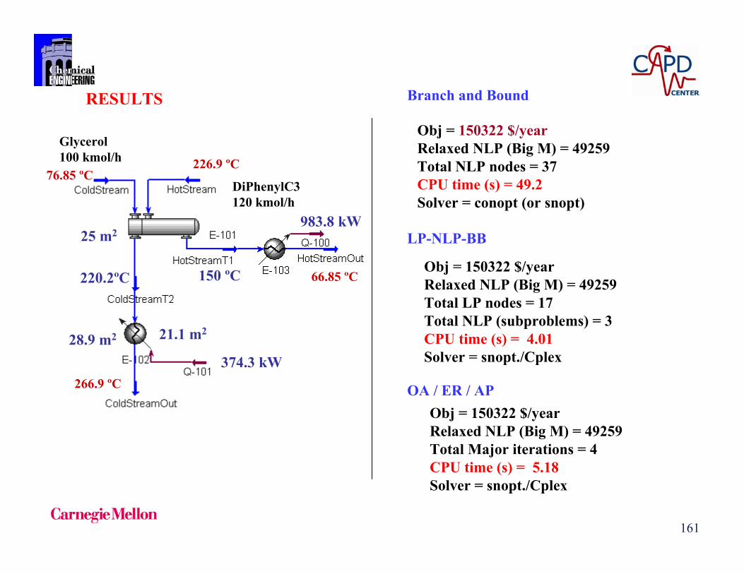
161

RESULTS

226.9 ºC

266.9 ºC

76.85 ºC

66.85 ºC

983.8 kW

374.3 kW

150 ºC220.2ºC

25 m2

28.9 m2 21.1 m2

Branch and Bound

Obj = 150322 $/yearRelaxed NLP (Big M) = 49259 Total NLP nodes = 37CPU time (s) = 49.2 Solver = conopt (or snopt)

LP-NLP-BB

Obj = 150322 $/yearRelaxed NLP (Big M) = 49259 Total LP nodes = 17Total NLP (subproblems) = 3CPU time (s) = 4.01Solver = snopt./Cplex

OA / ER / APObj = 150322 $/yearRelaxed NLP (Big M) = 49259 Total Major iterations = 4CPU time (s) = 5.18Solver = snopt./Cplex

Glycerol 100 kmol/h

DiPhenylC3120 kmol/h

162

100010)(

,,,

10010)(

,,,

_

101)(

,,,

AACCostTTTTfA

HeadFixed

AACCostTTTTfA

PipeMultiple

AACCostTTTTfA

PipeDouble

FHFH

outC

inC

outH

inH

MPMP

outC

inC

outH

inH

DPDP

outC

inC

outH

inH

Example 2. DME Plant

WaterCostCostACCost

UTTTTAA

WaterHE

CostACCost

UTTTTAA

CoolerAir

UtilityAir

TS

WWout

Win

sout

sin

UtilityAir

Air

AirAir

outAir

ins

outs

in

_)(

,,,,

_

0)(

,,,,

VaporCostCostACCost

UTTTTAA

HeadFloating

VaporCostCostACCost

UTTTTAA

ReboilerKettle

UtilityAir

FH

WR

outV

ins

outs

in

Utility

Kettle

AirR

outV

ins

outs

in

_)(

,,,,)(,,,,

261.5 kmol/h1.01 bar25 ºCxMeOH = 0.8xWater = 0.2

137.3 kmol/hxMeOH =0.995

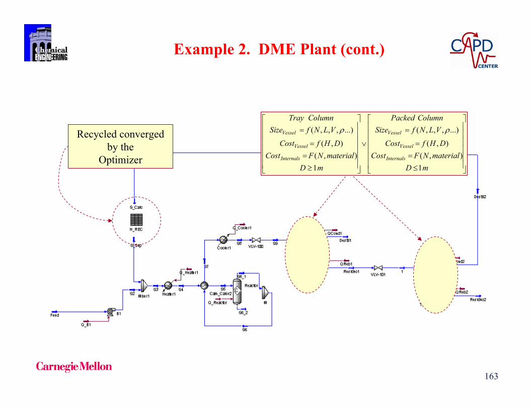
163

mDmaterialNFCost

DHfCost

VLNfSizeColumnPacked

mDmaterialNFCost

DHfCost

VLNfSizeColumnTray

Internals

Vessel

Vessel

Internals

Vessel

Vessel

1),(

),(

...),,,(

1),(

),(

...),,,( Recycled converged by the

Optimizer

Example 2. DME Plant (cont.)

164

Optimal Solution

Air 374.6 m2

M P 16.6 m2

FH 46.4 m2

FH 37.8 m2

FH 10.8 m2

Kettle 54.6 m2

Packed

Tray18.2 m2

6.344 kW

2.99 kW

4668 kW944 kW

2609 kW

1735 kW

3090 kWD = 0.93 mH = 8.4 m D = 2.94 m

H = 11.07 mN = 21 trays

10 m x 0.72 m

4549 kW

159.8 ºC48.62ºC260ºC

366ºC

281ºC

81.7ºC10.5 bar 173.3 kmol/h DME

x =0.995

1.1 bar15.5 bar65.7 ºC147.8 kmol/h

Water

TAC = 1.002x106 $/year

261.5 kmol/h1.01 bar25 ºCxMeOH = 0.8xWater = 0.2

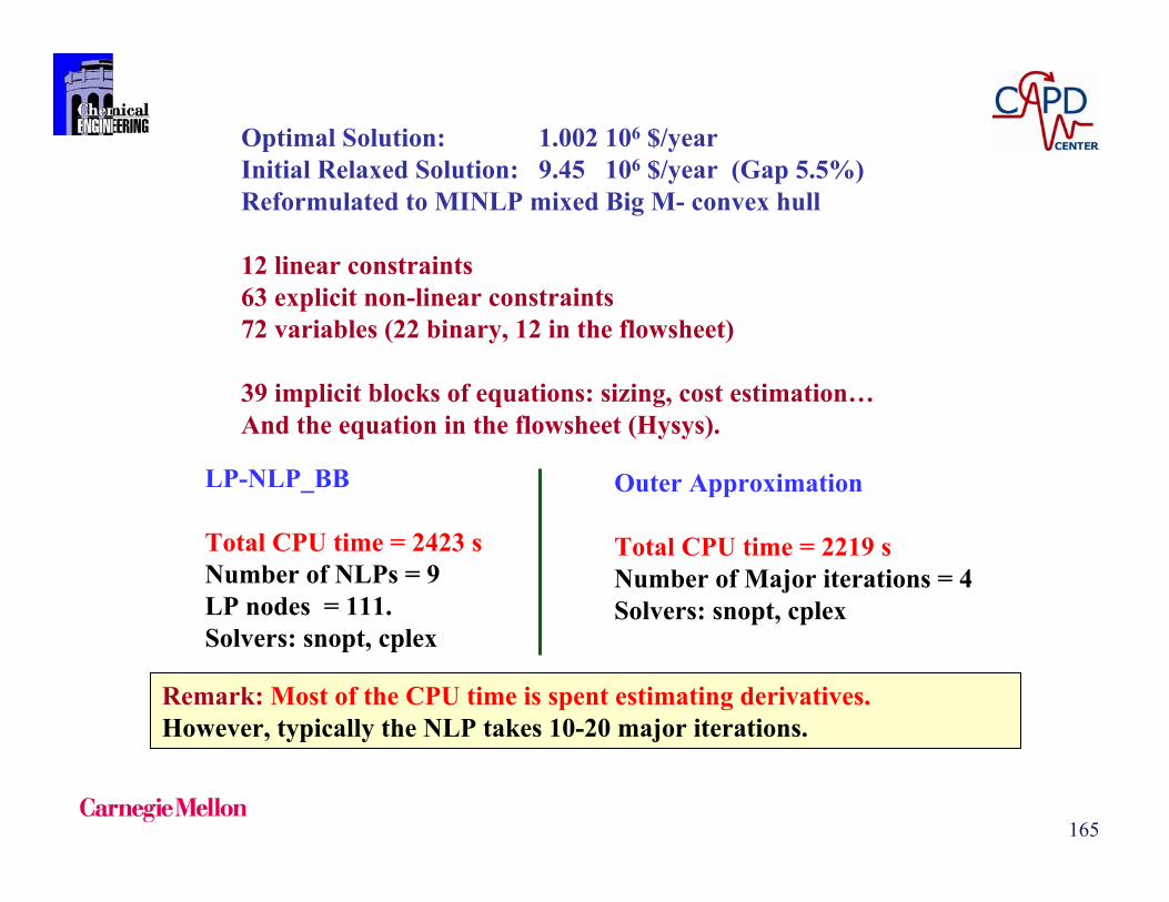
165

Optimal Solution: 1.002 106 $/year Initial Relaxed Solution: 9.45 106 $/year (Gap 5.5%)Reformulated to MINLP mixed Big M- convex hull

12 linear constraints63 explicit non-linear constraints72 variables (22 binary, 12 in the flowsheet)

39 implicit blocks of equations: sizing, cost estimation…And the equation in the flowsheet (Hysys).

LP-NLP_BB

Total CPU time = 2423 sNumber of NLPs = 9LP nodes = 111.Solvers: snopt, cplex

Outer Approximation

Total CPU time = 2219 sNumber of Major iterations = 4Solvers: snopt, cplex

Remark: Most of the CPU time is spent estimating derivatives.However, typically the NLP takes 10-20 major iterations.

166

Perform flowsheet synthesis using models from process simulators

Motivation

Black box models• No access to the original code• In some cases significant CPU

computation time is required• Usually derivatives are not available

In modular process simulators:• No derivative information available

• Usually perturbation does not provide accurate values due to the noise

introduced by the model

Rigorous Flowsheet Optimization using Process Simulators and Surrogate Models

Caballero, Grossmann (2008)

167

Kriging Interpolation:

( ) ( ) ( )y x f x Z x

Usually f(x) = μ ( ) 0E Z x

Kriging assumes that errors are not independent but a function of x

2cov ( ), ( ) ( , )i j i jZ Z x x R x x2 = Process Variance

, ,1

, exp

0; 0 2

ld P

i j l i l j ll

l lP

R x x x x Spatial correlation function : No Euclidean

Include adjustable parametersDue to these parameters it is not sensitive to the units of measurements

(a non interpolation version is easy to implement as well)

1new Ty x r R y 1

-1 222 -1-1

(1 )( ) 1T

new TTs x

r R rr R r1 R 1

The final predictor for the new point (xnew, ynew)

Standard error predicted by the interpolator

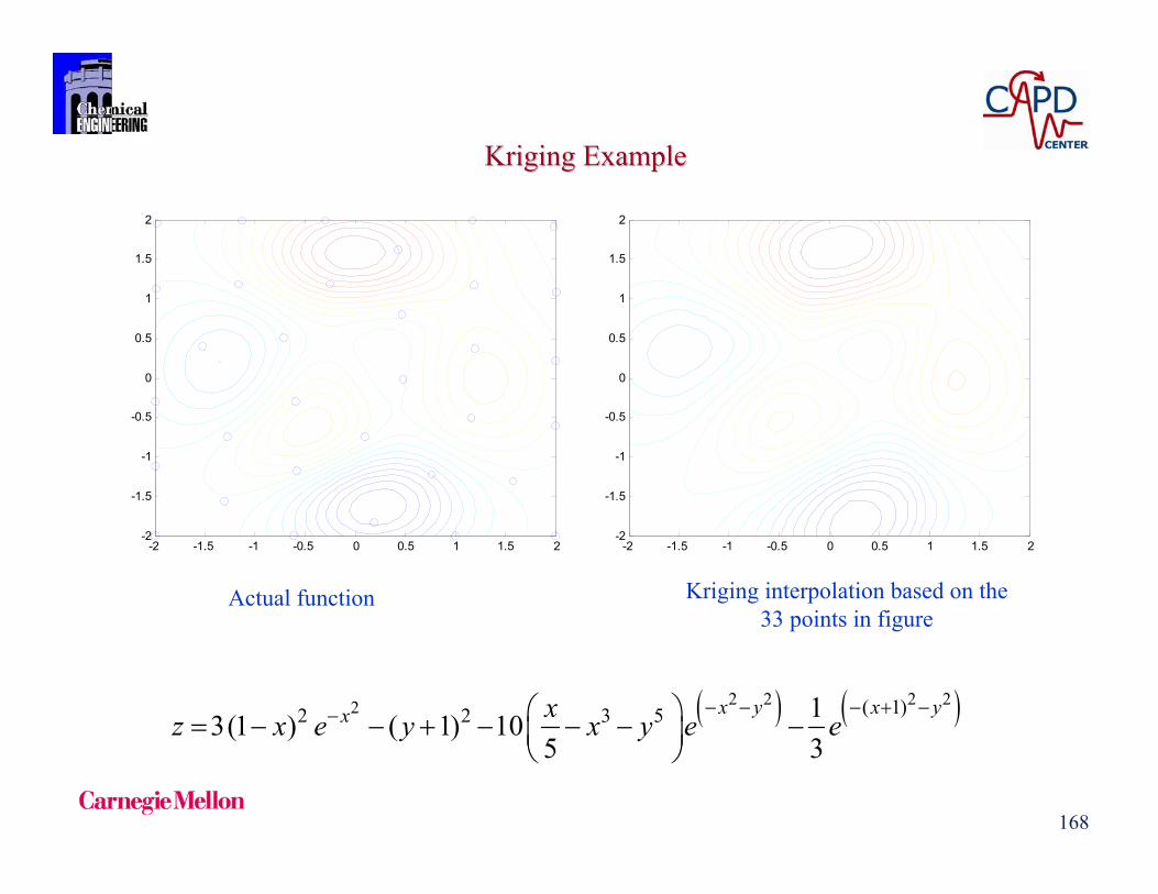
168

KrigingKriging ExampleExample

-2 -1.5 -1 -0.5 0 0.5 1 1.5 2-2

-1.5

-1

-0.5

0

0.5

1

1.5

2

-2 -1.5 -1 -0.5 0 0.5 1 1.5 2-2

-1.5

-1

-0.5

0

0.5

1

1.5

2

2 2 2 22 ( 1)2 2 3 5 13(1 ) ( 1) 105 3

x y x yx xz x e y x y e e

Actual function Kriging interpolation based on the 33 points in figure

169

-2-1

01

2

-2-1

0

12

-10

-5

0

5

10

-2-1

01

2

-2-1

0

12

-10

-5

0

5

10

-2-1

01

2

-2-1

0

12

-10

-5

0

5

10

KrigingKriging ExampleExample

Actual function Kriging interpolation

Errors predicted by the kriging

170

-2-1

01

2

-2

-10

12

-10

-5

0

5

10

-2-1

01

2

-2

-10

12

-10

-5

0

5

10

2 2 2 22 ( 1)2 2 3 5 13(1 ) ( 1) 105 3

x y x yx xz x e y x y e e

( , )z x yx

Analytical ( , )z x yx

Calculated by kriging

171

Algorithm

1. Select unit operation(s) to be substituted by a metamodel2. Bounds on variables (as tight as possible)3. Sampling

Latin Hypercube sampling, Hammersley, Halton o Sobol

The sampling must be done to preserve the uniformity of the distribution and avoid ‘correlation’.

,max min i ji j

d di,j = distance between sample points i and j

4. Generate kriging model Adjust parameters using an available NLP solver (SNOPT, CONOPT)

5. Validate kriging model : Cross validation

6. Optimization using the kriging metamodel instead of the selected unit operations(Using any NLP solver available i.e. SNOPT, CONOPT, KNITRO)

7. Refinement stage (optional):

8. Re-sampling and recalibration9. Repeat from point 6 until convergence

172

Example: phtalic anhydride from o-xylene

2 8 10 2 6 4 2 2o-xylene phthalic anhydride

2 8 10 4 2 3 2 2o-xylene

2 8 10 2 2o-xylene

( 1) 3 3 ( )

( 2) 7.5 4 4

( 3) 10 8 5

maleic anhydride

R O C H H O C H CO O

R O C H C H O CO H O

R O C H CO H O

Min : Total annual cost = Fixed + variable costs(compressor, pump, heater, cooler, reactor, flash, column)

s.t. cost and sizing equationsph. Anhydride > 0.99 (molar fraction)

Plug flow reactor substituted by krigingmetamodels

Number of sample points = 71 Convergence in two major iterationsTotal CPU time = 169.9 s. ; SOLVER = SNOPT7

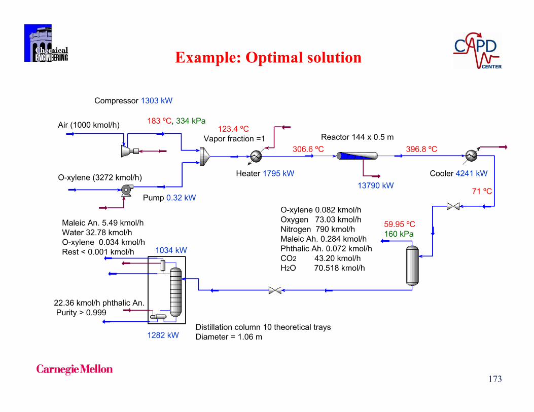
173

Air (1000 kmol/h)

O-xylene (3272 kmol/h)

Compressor 1303 kW

Pump 0.32 kW

183 ºC, 334 kPa123.4 ºC

Vapor fraction =1

Heater 1795 kW

306.6 ºC 396.8 ºCReactor 144 x 0.5 m

Cooler 4241 kW13790 kW

71 ºC

59.95 ºC160 kPa

O-xylene 0.082 kmol/hOxygen 73.03 kmol/hNitrogen 790 kmol/hMaleic Ah. 0.284 kmol/hPhthalic Ah. 0.072 kmol/hCO2 43.20 kmol/hH2O 70.518 kmol/h

Distillation column 10 theoretical traysDiameter = 1.06 m1282 kW

1034 kW

Maleic An. 5.49 kmol/hWater 32.78 kmol/hO-xylene 0.034 kmol/hRest < 0.001 kmol/h

22.36 kmol/h phthalic An.Purity > 0.999

Example: Optimal solution

174

Introduction & Motivation

The whole picture:

June 19, 2011 174

Solution

Design specifications

Unit variable analysis

Sets IS, DS

IS bounds

DS data generation

Data fitting

Surrogate model

Superstructure generation

Process design statement

DS space samples

Superstructure model

Complete superstructure model

Solver

Detailed unit models

Standard surrogate forms

Surrogate formulation

Process superstructure

IS space sampling

IS bounds update

Surrogate Model Generation

Superstructure Modeling

Surrogate Model Design .

Is space samplesHigh level

modeling

Results

Reformulation

IS Bounds initialization

Model solution

Henao, Maravelias (2010)

175

Synthesis of methanol in a fixed bed multi‐tube reactor:Reactions

Reactor model:o Adiabatic operation,o Total radial mix,o No axial diffusion,o Pressure drop as per Ergun,o Real mixture thermodynamics.

Motivation

)()(3

222

222

WGSHCOOHCOMSROHMeOHHCO

Dt = Tube internal diameterNt = Number of tubes

LR

TI, PI, FIxi]I, Fi]I

TO, PO, FO, xi]O, Fi]O

TFTO, PFTO, FFTOTFTI, PFTI, FFTI

rj – reaction rateh – molar enthalpyν – molar volumeμ - viscosity

R

FTFT

Rs

NC

iii

sppp

ppp

s

LP

dLdP

AsvF

vMx

DDdL

dP

,

Hydraulics

1

3

2

Rewhere

75.1Re

115011000

1

4

42

2

ttR

ttR

Rt

tR

DNAs

DN

LDNV

Geometry

NCi

dLdF

NCiLdAs

dFradVdF

FTi

R

iNR

jjij

R

i

,...,10

,...,1,1

Balances Mass

FTFTR

R

hFddLqhFddLq

balances Energy

NCivFFCNRjTCCfr

ii

NCj

,...,1/,...,1),,...,( 1

Kinetics

TTUq FT transferHeat

NCi

FFx

FF

FFx

FF

xFF

FT

FTiFTi

NC

iFTiFT

ii

NC

ii

ii

,...,1,, 11

relations

NC

NC

FTNCFTFTFTFT

NC

xxPTfxxPTfv

xxPTfhxxPTfh

,...,,,,...,,,

,...,,,,...,,,

1

1

1

1

propertiestransport and Thermo

176

Motivation

What we really need is a mapping: f: inputs outputs

2530

3540

4550

150

200

250

300150

200

250

300

350

PIN(bar)

Outlet temperatureature Vs. inlet Pressure-Temperature

TIN(°C)

T OU

T(°C

)

2530

3540

4550

150

200

250

3000

10

20

30

40

50

PIN(bar)

Outlet pressure Vs. inlet Pressure-Temperature

TIN(°C)

PO

UT(b

ar)

2530

3540

4550

150

200

250

300900

950

1000

1050

1100

1150

PIN(bar)

Outlet molar flow of CO Vs. inlet Pressure-Temperature

TIN(°C)

F CO(k

mol

/hr)

2530

3540

4550

150

200

250

3000

0.005

0.01

0.015

0.02

0.025

0.03

PIN(bar)

Outlet molar flow of H2O Vs. inlet Pressure-Temperature

TIN(°C)

F H2O

(km

ol/h

r)

2530

3540

4550

150

200

250

3005000

5200

5400

5600

5800

6000

PIN(bar)

Outlet molar flow of H2 Vs. inlet Pressure-Temperature

TIN(°C)

F H2(k

mol

/hr)

Our approach: Replace complex unit models with surrogate models,relating only necessary variables while enforcing the same constraints

177

Surrogate Model Design

First­principles unit model:IUM: Independent variable set (degrees of freedom),DUM: Dependent variable set,CUM: Connecting variable set (variables appearing in any other part of the problem),FUM: Fixed variable set (design specifications),

IUM

CUM

DUM

CUMFUM

Implicit unit model mapping(simulation)

Surrogate unit model:Enforce constraints between independent and connecting dependent variables

IS: Independent variable set,DS: Dependent variable set,

UMUMS F\II

UMUMUMUMS I\CDCD

ISDimensionally reduced surrogate model mapping

DS

178

Surrogate Model Design

Fixed (FUM) and connecting (CUM) variables are given from problem are givenThere are multiple choices for independent (IUM) variablesStructurally non‐singular model: perfect matching between dependent variables and equations†

Var1 Var2 Var3 Var4 Var5 Var6 Var7 Var8

Eq1 Eq2 Eq3 Eq4 Eq5

Unit model bipartite representation

† Bunus P. Fritzson P. Sim Tran Soc Mod & Sim Int 2004; 80: 321

Matching problem:J: Set of variables,K: Set of equations,A: Variable‐equation incidence matrix,xjk : Variable‐equation matching variablesyj : Selection binaries defining IUMwj : Selection preference coefficients

Since FUM IUM yj = 1, jFUMSelection preferences to reduce number of surrogate variables; include connecting (CUM) in IUM

J

K

A

A

j

k

,,yx

yx

x

s.t.

yw

jjk

jj,kk:

jk

j,kj:jk

Jjjj

10

1

1

max

UMUMS

UMUMS

I\CDF\II

UMUMUMS

UMUMS

ICCD

FII

UMC jwj 1

179

Surrogate Model Design

Var1 Var2 Var3 Var4 Var5 Var6 Var7 Var8

Eq1 Eq2 Eq3 Eq4 Eq5

Perfect matching between eqs. and DUM variables

Fixed (FUM) and connecting (CUM) variables are given from problem are givenThere are multiple choices for independent (IUM) variablesStructurally non‐singular model: perfect matching between dependent variables and equations†

† Bunus P. Fritzson P. Sim Tran Soc Mod & Sim Int 2004; 80: 321

Matching problem:J: Set of variables,K: Set of equations,A: Variable‐equation incidence matrix,xjk : Variable‐equation matching variablesyj : Selection binaries defining IUMwj : Selection preference coefficients

Since FUM IUM yj = 1, jFUMSelection preferences to reduce number of surrogate variables; include connecting (CUM) in IUM

J

K

A

A

j

k

,,yx

yx

x

s.t.

yw

jjk

jj,kk:

jk

j,kj:jk

Jjjj

10

1

1

max

UMUMS

UMUMS

I\CDF\II

UMUMUMS

UMUMS

ICCD

FII

UMC jwj 1

180

Surrogate Model Design: Example

Optimal design and operation of a homogeneous CSTR with fixed feed and ΔP

C

C

C

RR

C

RR

R

C

R

C

cc,OOOO

cc,OOOh

O

cc,IIIh

I

Oc,Oc,O

c,Oc

c,Oc,Oc,Ic

c,Ic,I

cc,OOr

ORI

cc,OOR

cc,II

c,Or

rr,cRc,I

O

CSTR

RRocObj

x,PT

x,PTh

x,PTh

c

xC

FFxFFx

rC,Tr

PPΔP

FhQFh

cFrνVFTT

ts

QVF

O

O

I

,f

,f

,f

micsThermodyna

,,

,f

sexpression Additional

balanceEnergy

,balances Mass

model detailedCSTR

0...f..

,,fmax

problemon optimizatiCSTR

rr

max

*,

Fc,ITI PI

Fc,OTO POVR

PR

ORRcc,III

RR,OcO

Rcc,III

TVPΔF,PTQVFT

PΔF,PT

,,,,,,,

,,

*

CUM

UM

CUM

IC

F

ORS

R,Oc

TVQF

,,*

IDS

181

Surrogate Model Formulations

We assume FUM =Ø, General considerations for IUM , CUM

Incorporate linear equations of the original unit models:

O

M

SC

O

M

S

M

SS

SU

SU

CU

Mixers Stream

I

I

OI

uscssc,s

Tus'

us's

s

sc,s

sc,s

s'u

,P,TFT

s'u

PP

cuFF

u

u

uu

,f

mapping bleMultivaria

,min

sexpression Additional

,

balances Mass

,s'

''

I1

IN O

O

I

S

S

O

I

S

S

S

SU

U

CS

SU

Splitters Stream

O

u

us's

s's

u

u

s's',u

c,s's',uc,s

s'

su

TTPP

u

cs'

su

ξ

FξF

u

,

sexpression Additional

,

,

1

balances Mass

IO1

ON

CPT

O

CPT

SC

SC

O

I

CPT

CPT

SS

U

SU

S

SU

CU

TurbinesPumpssCompressor

I

I

OI

u

s'u

,εΔP,P,TFW

,εΔP,P,TFT

s'

suPΔPP

cuFF

u

uuscssc,s

Wuu

uuscssc,s

Tus's'

u

u

s'us

sc,s

sc,s

u

u

uu

,,

,f

,f

mapping bleMultivaria

,

sexpression Additional

,

balances Mass

,

'' W

I O

W

I

O

182

Surrogate Model Formulations

FV

SC

O

FV

SC

O

I

FV

FV

SS

U

CS

U

S

SU

CU

Vessels Flash

I

I

OI

u,QPΔ,P,TFT

cos'

u,QPΔ,P,TFF

s'

su

TTPPP

cuFF

uuscsc,s

Tuu

1uuuscsc,s

Fc,s',uc,s'

u

u

sc,s

sc,s

u

u

uu

,,f

\,,f

mapping bleMultivaria

,

sexpression Additional

,

balances Mass

s

s

s'u

s'us

''

O

EV

SC

O

I

EV

EV

SS

SU

S

SU

CU

Valves Expansion

I

OI

uus

cssc,sT

us's'

u

us'us

sc,s

sc,s

s'u

PΔ,P,TFT

s'

su

PPΔP

cuFF

u

uu

,,f

mapping bleMultivaria

,

sexpression Additional

,

balances Mass

,

''

HC

SC

O

I

HC

HC

SS

U

S

SU

CU

Coolers-Heaters

I

OI

uPΔT,P,TFQ

s'

su

TTPPΔP

cuFF

uuscssc,s

Quu

u

us'u

s'us

sc,s

sc,s

u

uu

,,,f

mapping bleMultivaria

,

sexpression Additional

,

balances Mass

''

I O

Q

I O

Q

I O1

O2

We assume FUM =Ø, General considerations for IUM , CUM

Incorporate linear equations of the original unit models:

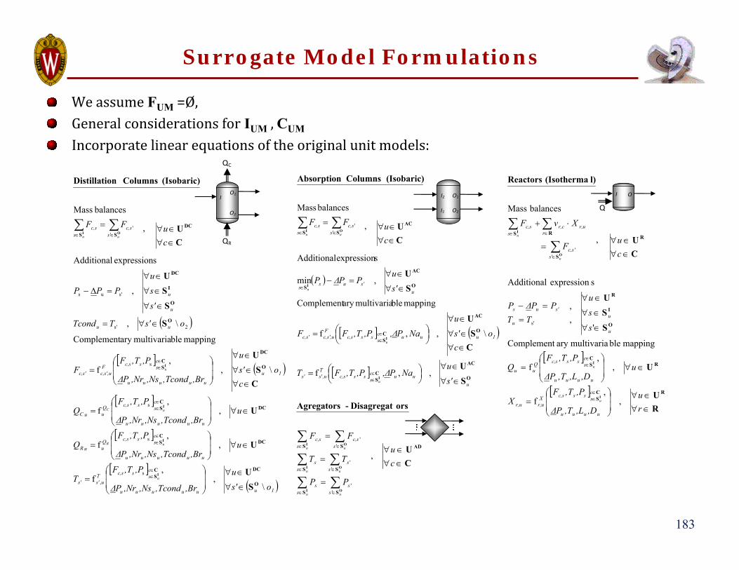
183

Surrogate Model Formulations

O

AC

SC

O

AC

SC

O

AC

S

AC

SS

SU

CS

U

SU

CU

(Isobaric) Columns Absorption

I

I

I

OI

uuus

cssc,sT

,uss'

1uuuscssc,s

Fc,s',uc,s'

us'us

s

sc,s

sc,s

s'u

NaPΔ,,P,TFT

cos'

uNaPΔ,,P,TFF

s'u

PPΔP

cuFF

u

u

u

uu

,,f

\,,f

mapping blemultivariaary Complement

,min

sexpression Additional

,

balances Mass

'

''

1uuuuuu

scsc,sT

us's'

uuuuu

scsc,sQ

uuR

uuuuu

scsc,sQ

uuC

1u

uuuuu

scsc,sF

c,s',uc,s'

uu

u

u

sc,s

sc,s

os'u

,Br,Tcond,Ns,NrPΔ

,P,TFT

u,Br,Tcond,Ns,NrPΔ

,P,TFQ

u,Br,Tcond,Ns,NrPΔ

,P,TFQ

cos'

u

,Br,Tcond,Ns,NrPΔ

,P,TFF

os'TTcond

s'

su

PPP

cuFF

u

uR

uC

u

uu

\,

,f

,,

f

,,

f

\,,

f

mapping blemultivariaary Complement

\,

,

sexpression Additional

,

balances Mass

s

,

s

s

s

2s'

s'us

''

O

DCSC

DCSC

DCSC

O

DC

SC

O

O

I

DC

DC

SS

SU

U

U

CS

U

S

S

SU

CU

(Isobaric) ColumnsonDistillati

I

I

I

I

OI

QR

QC

I O1

O2

O1

O2

I2

I1

RU

U

S

SU

CU

l)(Isotherma Reactors

RSC

RSC

O

I

R

R

S

RS

I

I

O

I

ru

,D,L,TPΔ

,P,TFX

u,D,L,TPΔ

,P,TFQ

s

su

TTPPΔP

cu

F

XνF

uuuu

scssc,sX

r,ur,u

uuuu

scssc,sQ

uu

u

uu

s'us

sc,s

rr,ur,c

sc,s

u

u

u

u

,,

f

,,

f

mapping blemultivariaary Complement

',,

sexpression Additional

,

balances Mass

s'

''

Q

I O

CU

orsDisagregat-Agregators

AD

SS

SS

SS

OI

OI

OI

cu

PP

TT

FF

uu

uu

uu

ss

ss

ss

ss

sc,s

sc,s

,

''

''

''

We assume FUM =Ø, General considerations for IUM , CUM

Incorporate linear equations of the original unit models:

184

Data Generation and Training

The framework can be used with any fitting methodLinear models: fit split fraction, extend of reaction, etc.Shortcut methods: fit key parameters

We use artificial neural network (ANN) surrogates:Simple structure and excellent fitting capabilities.Reformulation propertiesNetwork with a total of K layers

Formulation:u0: network inputuK: network output

function activation layer f vectorbias layer

matrix weight layer output ayer where

,...,1,f

kkk

klKk

k

k

k

k

kkkkk

bWu

buWu 1

u10

u20

…

un00

w1,11

…

w2,11

wn1,11

w1,21

w2,21

wn1,21

w1,n01

w2,n01

wn1,n01

b11

b21

bn11

f()

f()

f()

u11

u21

un11

…

w1,12

…

w2,12

wn2,12

w1,22

w2,22

wn2,22

w1,n12

w2,n12

wn2,n12

b12

b22

bn22

f()

f()

f()

u12

u22

un22

…

…

…u1K-1

u2K-1

…

un(k-1)K-1

w1,1K

…

w2,1K

wnK,1K

w1,2K

w2,2K

wnK,2K

w1,n(K-1)K

w2,n(K-1)K

W2n(K-1),nKK

b1K

b2K

Bn(K)K

f()

f()

f()

u1K

u2K

Un(K)K

Layer 1 Layer 2 Layer K

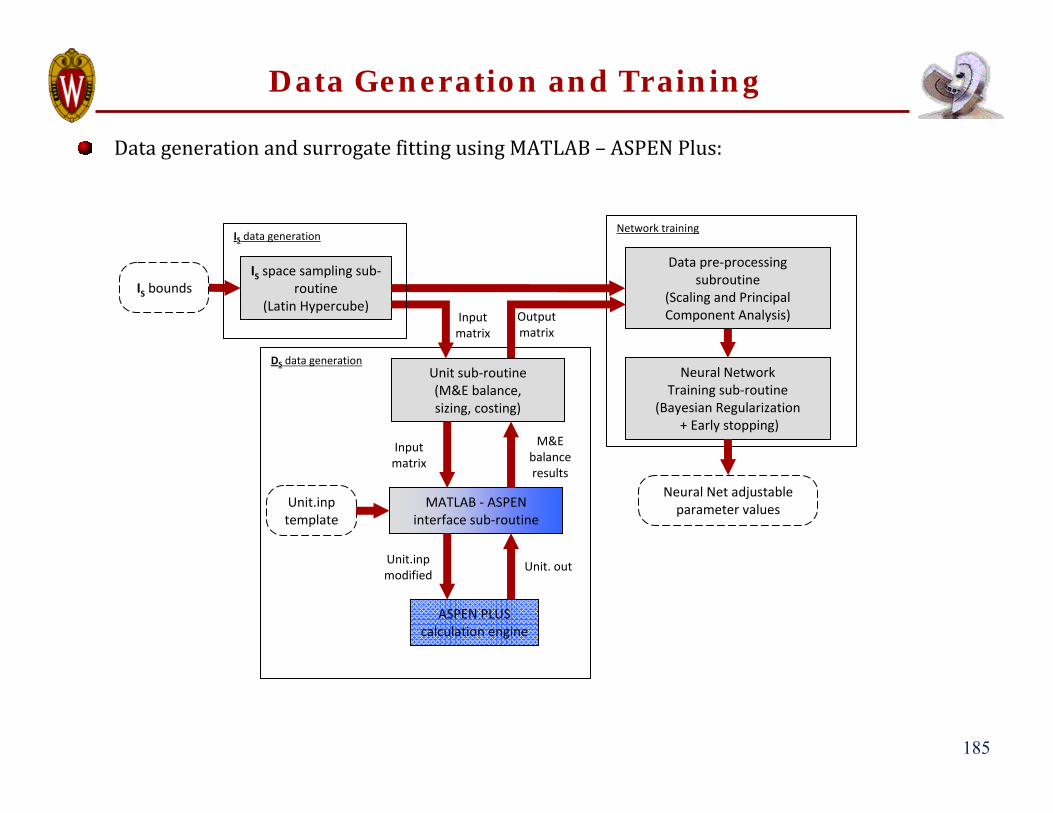
185

Network training

Data Generation and Training

Data generation and surrogate fitting using MATLAB – ASPEN Plus:

Unit.inpmodified

Unit. out

Inputmatrix

IS bounds

Neural Net adjustable parameter values

Outputmatrix

Inputmatrix

M&E balance results

DS data generation

Data pre‐processing subroutine

(Scaling and Principal Component Analysis)

MATLAB ‐ ASPEN interface sub‐routine

ASPEN PLUS calculation engine

Unit.inptemplate

IS space sampling sub‐routine

(Latin Hypercube)

Neural Network Training sub‐routine

(Bayesian Regularization+ Early stopping)

Unit sub‐routine(M&E balance, sizing, costing)

IS data generation

186

Optimum design and operation of a homogeneous CSTR,Production of Maleic Anhydride,

Fixed feed Fc,I ,TI, PI and pressure drop P,Objective: Find VR and TO maximizing profit

Variable analysis:

Data Generation and Training: Example 1

Fc,ITI PI

Fc,OTO POVR

PR

ORRCcIc,II

RROc*,O

RCcIc,II

T,V,PΔ,F,P,TQ,V,F,T

PΔ,F,P,T

UM

UM

UM

IC

F ORS

R,Oc

TVQF

,,*

IDS

OHCOOHCOHCOOOHC

OHCOOHCOHC

22266

222324

22324266

365.743

225.4

Original model: |IUM|+|DUM|= 45, |FUM|= 9Surrogate model: |IS|+|DS|= 4

Surrogate: ANN with 2 hidden layers, 5 neurons each

0

20

40

400500600700

800900

-2

0

2

4

6

8

TO[K]VR[m3]

Original modelSurrogate model

FAM]O [kmol/h]Optimum values:• TO[K] = 670• VR[m3] = 40

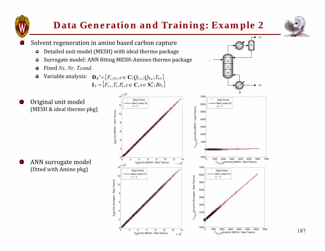
187

Data Generation and Training: Example 2

Solvent regeneration in amine based carbon captureDetailed unit model (MESH) with ideal thermo packageSurrogate model: ANN fitting MESH‐Amines thermo packageFixed Ns, Nr, Tcond.Variable analysis:

uusc,sS

OuRuCc,O

Brsc,P,TFTQQcF

;,,;;;,' 12

IS

SCICD

s

1

2

3

4

5

I

O1

O2

Original unit model(MESH & ideal thermo pkg)

ANN surrogate model(fitted with Amine pkg)

0 1000 2000 3000 4000 5000 6000 7000-1000

0

1000

2000

3000

4000

5000

6000

7000

FCO2,O2[kmol/hr] (MESH - Real Thermo)

F CO 2,O

2[km

ol/h

r] (S

urro

gate

- R

eal T

herm

o)

Data PointsBest Linear FitY = T

0 2 4 6 8 10 12 14

x 109

0

2

4

6

8

10

12

14x 109

QR[kJ/hr] (MESH - Real Thermo)

QR[k

J/hr

] (S

urro

gate

- R

eal T

herm

o)

Data PointsBest Linear FitY = T

0 1000 2000 3000 4000 5000 6000 7000-1000

0

1000

2000

3000

4000

5000

6000

7000

FCO2,O2[kmol/hr] (MESH - Real Thermo)

F CO 2,O

2[km

ol/h

r] (M

ES

H -

Idea

l The

rmo)

Data PointsBest Linear FitY = T

0 2 4 6 8 10 12 14

x 109

0

2

4

6

8

10

12

14x 109

QR[kJ/hr] (MESH - Real Thermo)

QR[k

J/hr

] (M

ES

H -

Idea

l The

rmo)

Data PointsBest Linear FitY = T

188

High-level Formulation Approach

Generate superstructure (engineering judgment, artificial intelligence, evolutionary design)Choose method to activate/de‐activate unit models

Math programming with equilibrium constraints (Biegler et al.)Disjunctive programming (Grossmann et al.)

Reformulate into a mathematical programStandard methods can be used for linear equationsReformulation of nonlinear equations (mapping) is challenging (Stubbs & Merhotra, Grossmann et al.)

ANN reformulationNo variable transformationNo binaries in nonlinear eqstanh(0) = 0

JJ

JJJ

J

jjxg

jUx

cxx

cxgY

j

jj

jj

jjj

jj

j

j

j

j

j

j

,1,0,0

,0

,

0

C

S

SC

SC

U

ψ

SC

ψψ

ψψ

u

OPCCC

sc

PTF

Y

OPCPTCC

PTFgPTFhY

uu

u

u

s

s

sc

u

uCOPuu

usssCCuu

uscssscu

uscssscu

u

u

u

u

0,0000

0

,,

0,,,0,,, ,

,

,

ff

1,0

)tanh(

00)tanh()(

1

111

111

yyy

yY

fY

kkk

kkkk

kk

k

k

kkkk

kkk

UuLbuWv

vu

vu

buWvvvu

189189

What next for Process Synthesis and Design?

Three major issues:

1. Uncertainty:Theory is available (stochastic programming, robust optimization, flexibility analysis)Major issue: computational

2. Process intensificationLimited cases process flowsheets, microsytemsMajor issue: represenations

3. Nonlinear process modelsTo support process synthesis with complex modelsMajor issue: convergence

190

Process Intensification:Original Methyl Acetate Flowsheet

Water

Acetic Acid

Azeo

MethanolCatalyst

MethylAcetate

Solvent

Solvent/Entrainer

Water

HeaviesWater

Siirola (1988)

191

ExtractiveDistillation

Task F

DistillationTask G

ReactiveDistillation

Task EReactionTask AReactive

DistillationTask B

DistillationTasks

C and D

Acetic Acid

Catalyst

Methanol

Methyl Acetate

Water

Process IntensificationSingle Column Methyl Acetate Process

S S

ABC

Mixing CrystallizationReaction Drying

1 2 3 4

ABC

S

Unit 1 Unit 2 Unit 3 Unit 4 Unit 5Cast Iron

w/ AgitatorStainless Steel

w/ AgitatorCast IronJacketed

Stainless SteelJacketed w/ Agitator

TrayDryer

More than 100 alternatives: each requires nonlinear optimization

Equipment

Tasks

Synthesis Multiproduct Batch Plant(Lee, Grossmann, 2000)

p

j

N

iLii

Piii

PTt

itjij

Piti

T

t

jj

M

jj

EQ

j

HTn

NiQBn

MjNiptyptTtNiSBVts

CSCN

1

1

,...,1

,...,1;,...,1,...,1;,...,1..

COSTmin

Synthesis Multiproduct Batch Plant

Tt

jjptyptpty

VVY

Jj

itj

T

ititj

T

tj

tj

t

',0'

Objective function

Process time

Disjunction forTask Assignments

Nonconvexfunctions

Sizing

Demand

Horizon time

Nonconvex GDP Model

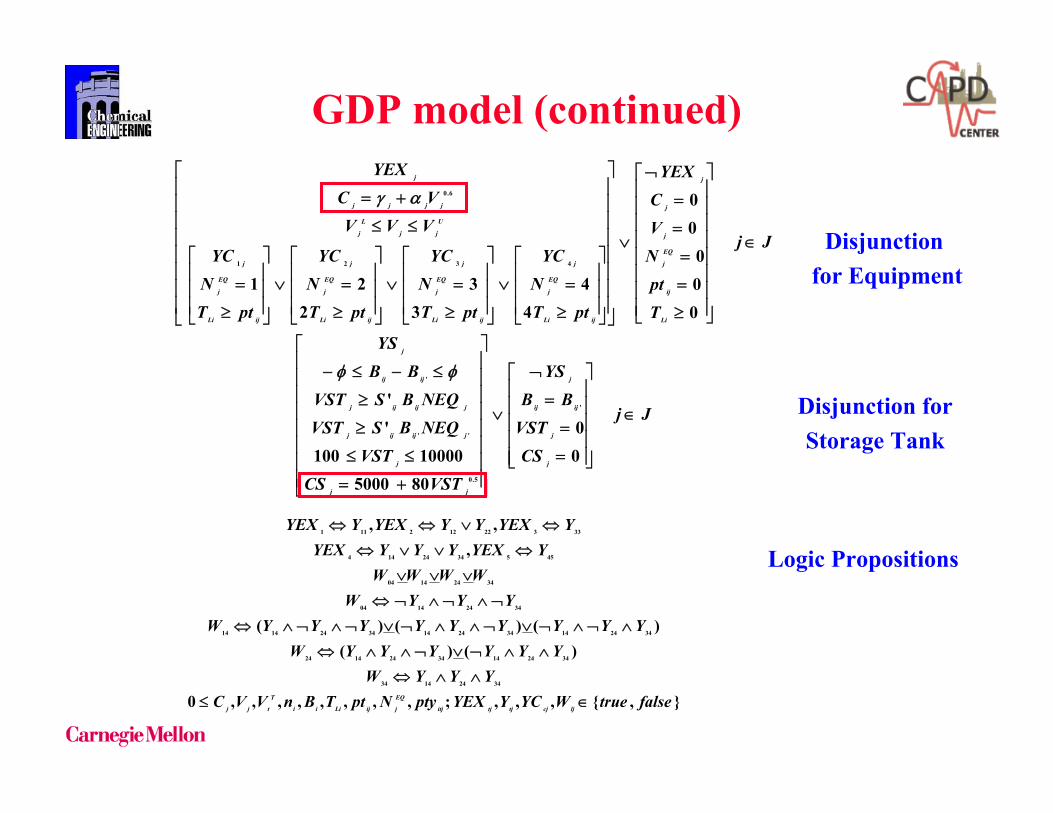
,,,,;,,,,,,,,0

)()()()()(

,,,

34241434

34241434241424

34241434241434241414

34241404

34241404

4553424144

33322122111

falsetrueWYCYYEXptyNptTBnVVCYYYW

YYYYYYWYYYYYYYYYW

YYYWWWWW

YYEXYYYYEXYYEXYYYEXYYEX

ljcjtjtjitj

EQ

jijLiii

T

tjj

Jj

CSVST

BBYS

VSTCSVST

NEQBSVSTNEQBSVST

BBYS

Jj

Tpt

NVC

YEX

ptTN

YC

ptTN

YC

ptTN

YC

ptTN

YC

VVVVC

YEX

j

j

ijij

j

jj

j

jijijj

jijijj

ijij

j

Li

ij

EQ

j

j

j

j

ijLi

EQ

j

j

ijLi

EQ

j

j

ijLi

EQ

j

j

ijLi

EQ

j

j

U

jj

L

j

jjjj

j

00

80500010000100

''

000

00

44

33

221

'

5.0

''

'

4321

6.0

Disjunction for Equipment

Disjunction forStorage Tank

Logic Propositions

GDP model (continued)

Proposed Algorithm for Nonconvex GDP

Nonconvex MINLPStep 0

ZU

OA (Viswanathan and Grossmann, 1990)

BoundContraction

New Bound

Step 1 (Zamora and Grossmann, 1999)

BB with Y’sUpdate ZL

Spatial BB

When solution is Integral

Update ZU

Stop whenZL ZU

Add Integer Cut

Fixed Y’s

Step 2

Step 3

(Lee and Grossmann, 2000)

(Quesada and Grossmann, 1995)

• Procedure (Lee and Grossmann, 1999) Relaxed NLP problem is solved. Check Infeasibility of each term.

• Branching Rule Select a term with Minimum Infeasibility

first. Logic Inference – fixes additional Boolean

Variables.

• Lower Bound is updated

• When all the Boolean variables are fixed and the relaxation gap is nonzero: switch to Spatial Branch and Bound.

Step 2: Disjunctive Branch and Bound

NLP

NLPNLP

Fix a termin disjunction

Convex hullremaining terms

Yj Yj

ZL

• Fixed Boolean Variables: Convex NLP Check the relaxation gap of each

underestimator function. Select the constraint with maximum

gap. Branch on a variable which causes the

maximum gap. Bisection Rule: Feasible region is

divided into 2 subregions. If the gap is small enough, an upper

bound is updated.

• Return to Step 2 with: Updated Global Upper Bound Feasibility Cut, Z < GUB Integer Cut for the chosen set of Y’s

Step 3: Spatial Branch and Bound

Nonconvex Objective Function f

x

GLB

Initial Region

Subregion 1 Subregion 2

0f2f

1f

Quesada and Grossmann (1995)

Upper Bound Solution

• Use 4 Stages (6 units) without Storage Tank

j = 1 j = 4 j = 5

Mixing Reaction

ABC

V1 = 4,842 L V2 = 2,881 L V4 = 2,469 L V5 = 8,071 L

DryingCrystallization

ABC

j = 2

2

8

4

9

A 243 batches, 4.5hrs

2

4

3

12

B 260 batches, 6hrs

7

4

9

3

C 372 batches, 9hrs 6000 hrs

1093 hrs 1562 hrs 3345 hrs

Cost = $ 277,928 (by GAMS/DICOPT++)

S

Mixing Reaction Storage Tank

ABC

j = 2 j = 3 j = 5V2 = 4,309 L VST2 = 4,800 L V3 = 3,600 L V5 = 11,753 L

DryingCrystallization

ABC

9 12 3

Global optimal cost = $ 264,887 (5% improvement) 3 Stages + 1 storage tank (5 units)

167 batches, 9hrs

184 batches, 12 hrs

255 batches, 9hrs

10

4

A 250 batches, 5hrs

6

3

B 293 batches, 3hrs

11

9

C 418 batches, 5.5hrs 6000 hrs

Storage 1503 hrs 2202 hrs 2295 hrs

Optimal Solution: Multiproduct Batch Plant

Environmentally Conscious Design and Planning of Hydrogen Supply Chains for Vehicle Use

Guillén-Gosálbez, Mele and Grossmann (2009)

Objective: Develop a framework for the design of infrastructures for producing and delivering H2

Cover the entire supply chain (holistic view of the system)

Include environmental concerns along with traditional economic criteria

Develop an efficient solution method

Motivation• Motivation for the adoption of hydrogen:

Reduces well-to-wheel GHG gases emissions (Hugo et al., 2006)

• Major obstacle to achieve the hydrogen transition (Jensen and Ross, 2000)

Developing an efficient infrastructure for producing and delivering hydrogen

Basis: case study by A. Almansoori and N. Shah (2006) in UK

Design of SCs for hydrogen production

Problem statement

• Given are: Demand of hydrogen Investment and operating costs Available technologies and potential locations (i.e., grids) GHG emissions associated with the SC operation

• The task is to determine the optimal SC configuration

• In order to minimize cost and environmental impact

?

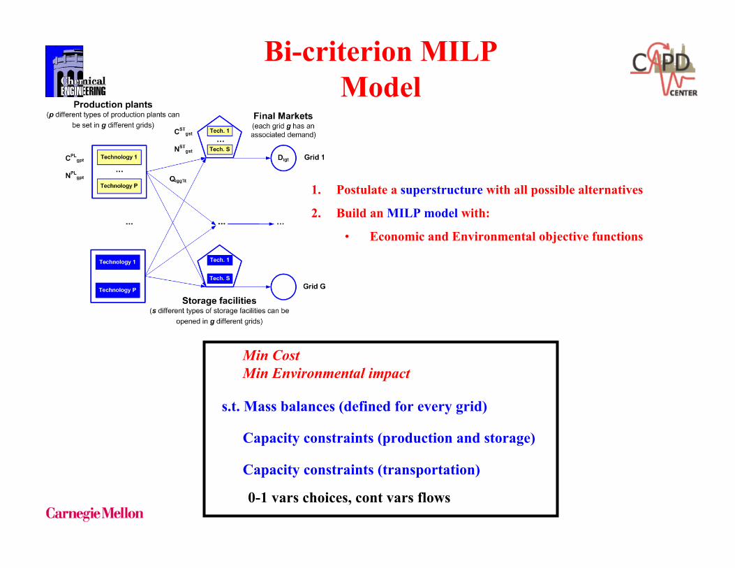
Bi-criterion MILP Model

1. Postulate a superstructure with all possible alternatives

2. Build an MILP model with:

• Economic and Environmental objective functions

s.t. Mass balances (defined for every grid)

Capacity constraints (production and storage)

Capacity constraints (transportation)

Min CostMin Environmental impact

0-1 vars choices, cont vars flows

Life Cycle Analysis-LCA (ISO 14040 series on LCA)

Life Cycle Analysis-LCA (ISO 14040 series on LCA)

Objective strategy to evaluate the environmental loadsassociated with a product, process or activity

Objective strategy to evaluate the environmental loadsassociated with a product, process or activity

by quantifying energy and materials used and waste released

by quantifying energy and materials used and waste released

It includes the ENTIRE LIFE CYCLE of the productIt includes the ENTIRE LIFE CYCLE of the product

to evaluate opportunities to do improvements

to evaluate opportunities to do improvements

Combine LCA with optimization tools(Azapagic et al., 1999, Mele et al., 2005,Hugo and Pistikopoulos, 2005)

Environmental aspects based on LCA (Eco-Indicator 99)

2. Translate emissions into damage (damage to human health caused by climate change)

• Human health: DALYs (Disability Adjusted Life Years)

Damage factors translate life cycle inventory into impact

Transportation tasks

Production (raw materials, energyconsumption and direct emissions)

1. Calculate the GHG emissions (Life Cycle Inventory: analysis from the cradle to the grave)

Storage (compression of hydrogen)

Environmental damage assessment: Global warming

Environmental Impact

Cost

Bi-criterion MILP with economic and environmental concerns

Pareto-optimal solutions: Epsilon constraint methodSolve a set of single objective problems for different values of ε

Solution strategy: Epsilon constraint

Environmental improvements are achieved through technological and topological changes

• Replace steam reforming by biomass• Do not use compressed gaseous

hydrogen (too expensive)

Pareto set of alternative solutions

Extreme solutions

MINIMUM COST: more centralized network (economies of scale)

MINIMUM IMPACT: more decentralized network (reduces transportation emissions)

Decentralized networks decrease the environmental impact

208208

Concluding Remarks

1. Process synthesis: challenging problem that lies at heart of design and that is key to address sustainability problems

2. Process synthesis has greatly advanced in representationsand optimization methodologies

3. Advances in mixed-integer/disjunctive programming have provided a powerful framework for addressing synthesis problems

4. Many problems can be effectively addressedHENs, Water networks, steam and power plants, separations systemsProcess flowsheets

5. Challenges: uncertainty, process intensification, nonliner modeling