Advances in Agriculture for Doubling of Farmer’s Income
144
Shampi Jain Neeraj Verma Advances in Agriculture for Doubling of Farmer’s Income
Transcript of Advances in Agriculture for Doubling of Farmer’s Income

Shampi Jain
Neeraj Verma
Advances in Agriculture for Doubling of Farmer’s Income

An AKS University Initiative
Advances in Agriculture for Doubling of Farmer’s Income
India | UAE | Nigeria | Uzbekistan | Montenegro

An AKS University Initiative
Advances in Agriculture for Doubling of Farmer’s Income
Shampi Jain
Neeraj Verma

First Impression: 2020
Advances in Agriculture for Doubling of Farmer’s Income
ISBN : 978-81-946373-1-8
Rs. 650/- ( $18 )
No part of the book may be printed, copied, stored, retrieved, duplicated and reproduced in any form without the written permission of the author/publisher.
DISCLAIMER Information contained in this Edited book has been published by Empyreal Publishing House and has been obtained by the author(s) from sources believed to be reliable and are correct to the best of his/her knowledge. The author(s) are solely responsible for the contents of the articles compiled in this book. Responsibility of authenticity of the work or the concepts / views presented by the author through this book shall lie with the author. The publisher or editors do not take any responsibility for the same in any manner. Errors, if any, are purely unintentional and readers are requested to communicate such error to the Editors to avoid discrepancies in future. Published by: Empyreal Publishing House

IV
Preface
Though agriculture accounts for as much as a quarter of the Indian economy and employs an estimated 60 percent of the labor force, still it is considered highly inefficient, wasteful, and incapable of solving the hunger and malnutrition problems. Despite progress in this area during the last two decades, these problems have continued to frustrate India.
Apart from various problems faced by the Indian farmers, some important ones are instability and Fluctuations of weather, Poor Farming Techniques and Agricultural Practices, Inadequate Use of Inputs, Inadequate Irrigation Facilities, Absence of Crop Rotation, Lack of Organized Agricultural Marketing and Instability in Agricultural Prices.
Hon’ble Prime Minister of India, Shri Narendra Modi has called for doubling farmer’s income by 2022. To find out the solutions for the problems faced by the famers or the persons engaged in practices related to agriculture is a very complex one. Because in agriculture most of the things are interlinked with each other. Therefore a concrete multidimensional steps should be formulated for reducing the cost and increasing the income of the farmers significantly. Biotechnology along with sustainable agriculture could be a solution for increasing the farmer’s income. Therefore, In order to address the emerging challenges and for doubling farmer’s income over the next 4 years, a three days national conference was organized from 5-7 Sept., 2019 at AKS University, Satna with a theme of Biotechnology and Sustainable Agriculture for Doubling of Farmer’s Income by 2022.
Editors

V
Acknowledgements
We are pleased to present the papers presented during the national conference “Biotechnology and Sustainable Agriculture for Doubling of Farmer’s Income by 2022” held on 5-7 Sept., 2019. A large number of papers were received during the conference from various academicians, scientists and researchers covering various themes of the conference. These papers were thoroughly reviewed and edited in the form of book chapters. We are thankful to all participants to make it a grand success.
The present book with full papers shall provide an opportunity to the academicians, scientists and researchers, students and farmers to get the state of the art information on latest technologies to improve the farming system in agriculture.
The financial support from National Bank for Agriculture and Rural Development (NABARD), Madhya Pradesh Council of Science & Technology (MPCST), KJS Cement, Satna and academic support from SBBS, Allahabad to organize this conference is gratefully acknowledged. The support in all aspects from Er. Anant Soni, ProChancellor and Chairman AKS University, in organizing the conference and publishing of this book is duly acknowledged.
Sponsored by Madhya Pradesh Council of Science & Technology (MPCST)
National Bank for Agriculture and Rural Development (NABARD) Co sponsored by KJS Cement, Satna Academic Partners SBBS, Allahabad

VI
Table of Contents
Preface Acknowledgement
IV
V
Table of Contents VI - IX
Chapter - 1
PERFORMANCE OF RICE VARIETIES TO APPLIED NITROGEN UNDER IRRIGATED CONDITIONS
Rajesh Kumar Arya, R.K. Tiwari, Manoj Kumar Choudhari, R.M. Mishra, and K.N. Namdeo
1 - 5
Chapter - 2
EFFECT OF DIFFERENT SOURCES OF NUTRIENTS ON HYBRID RICE UNDER CENTRAL UP CONDITIONS
Ashutosh Gupta and R.K. Pathak
6 – 10
Chapter - 3
INTEGRATED NUTRIENT MANAGEMENT ON GROWTH, YIELD AND ECONOMICS OF KODO MILLET (PASPALUM SCROBICULATUM L.)
Manoj Kumar Choudhari, R.K. Tiwari, R.M. Mishra and K.N. Namdeo
11 – 14
Chapter - 4
PERFORMANCE OF INTEGRATED FARMING SYSTEM MODELS FOR IMPROVING PROFITABILITY AND LIVELIHOOD OF MARGINAL FARMERS OF KAWARDHA DISTRICT OF CHHATTISGARH
C.K. Chandrakar, M.C. Bhambari, Sanjeev Singh and K.K. Pandey
15 – 17
Chapter - 5
COMPARATIVE PERFORMANCE OF DIFFERENT SEED BED CONFIGURATIONS IN SOYBEAN CULTIVATION IN MANDSAUR DISTRICT OF MADHYA PRADESH
Rajesh Gupta, Akhilesh Singh, Rupak Kumar and Ajeet Sarathe
18 - 22
Chapter - 6
ASSESSMENT OF CROP WATER REQUIREMENT FOR VEGETABLE CROP OVER UTTAR PRADESH USING CROPWAT MODEL
Shashank Kumar, Lakshmi Prasanna Aggile, Himani Bisht and Shweta Gautam
23 – 29
30 - 34

VII
Chapter - 7
MODEL DEVELOPMENT FOR YIELD FORECASTING THROUGH PRINCIPAL COMPONENT ANALYSIS AND STEPWISE REGRESSION ANALYSIS FOR PIGEON PEA CROP ON CHHATTISGARH PLAIN ZONE
K.K. Pandey, Gaind Lal, Bhashkar and Yogesh Chelak
Chapter - 8
PRE HARVEST FORECASTING MODEL DEVELOPMENT BY PRINCIPAL COMPONENT ANALYSIS FOR PIGEON PEA ON MAHASAMUND DISTRICTS
Gaind lal, K.K. Pandey, Bhashkar and Upendra Naik
35 – 37
Chapter - 9
BIOLOGICAL CONTROL OF PARTHENIUM HYSTEROPHORUS (GAJAR GHAS) USING ZYGOGRAMMA BICOLORATA (MEXICAN BEETLE) IN CHITRAKOOT (U.P.)
Ramesh Chandra Tripathi and Preeti Tripathi
38 – 42
Chapter - 10
RATIONAL APPROACHES FOR THE MANAGEMENT OF PARTIAL ROOT PARASITE (STRIGA ASIATICA L. KUNTZE) IN KODO MILLET
A.K. Jain, Ruchi Chaurasia and R.P. Joshi
43 – 47
Chapter - 11
INFLUENCE OF DIFFERENT IRRIGATION AND FERTIGATION LEVELS ON GROWTH AND YIELD OF GARLIC UNDER DRIP FERTIGATION SYSTEM
Rajesh Gupta and M.K. Hardaha, Vijay Singh and Ajeet Sarathe
48 – 53
Chapter - 12
PERFORMANCE EVALUATION OF RIDGE AND FURROW SYSTEM ON THE GROWTH AND YIELD CHARACTERS OF SOYBEAN IN MALWA REGION OF MADHYA PRADESH
Rajesh Gupta, A.L. Basediya, Rajesh Kumar Mishra and Ajeet Sarathe
54 – 58
Chapter - 13
COMBINE EFFECT OF GIBBERELLIC ACID AND PLANT SPACING ON CORMS ATTRIBUTES OF GRANDIFLORAS L.) Cv. SNOW PRINCES GLADIOLUS (GLADIOLUS
Nag, K., Singh, A.R. and Singh, A.
59 – 62

VIII
Chapter - 14
EFFECT OF APPLICATION OF PHOSPHORUS AND MICRO NUTRIENTS ON GROWTH, YIELD AND QUALITY PARAMETERS OF SWEET ORANGE (CITRUS SINENSIS L.) CV. MOSAMBI
Purnima Singh Sikarwar, K.S. Tomar and Balaji Vikram
63 – 67
Chapter - 15
LEVEL OF KNOWLEDGE ON VEGETABLE PRODUCTION TECHNOLOGIES OF KVK TRAINED VEGETABLE GROWERS
Aditya Kumar Malla and Jeebanjyoti Behera
68 – 70
Chapter - 16
STRATEGIES FOR DOUBLING FARMER’S INCOME BY 2022 IN BUNDELKHAND REGION OF MADHYA PRADESH
Ashish Kumar Tripathi
71 – 75
Chapter - 17
ASSESS THE IMPACT OF PRADHAN MANTRI KRISHI SINCHAYEE YOJANA ON COST, RETURN, PRODUCTION AND PRODUCTIVITY OF WHEAT CROP IN SATNA DISTRICT OF MADHYA PRADESH
Rajeev Rav Suryvanshi and J.K. Gupta
76 – 79
Chapter - 18
AN ECONOMIC ESTIMATION OF CAPSICUM PRODUCTION IN SHAJAPUR DISTRICT OF MADHYA PRADESH
Pradeep Kumar Patidar, P.R. Pandy, J.K. Gupta and Trapti Pawaiya
80 – 90
Chapter - 19
MARKET LED EXTENSION- A PROFIT MAXIMIZATION TREND OF FARMING COMMUNITY
Pooja Jena and Manohar Saryam
91 – 98
Chapter - 20
ECONOMIC ANALYSIS OF INCOME AND EMPLOYMENT GENERATION ON INTEGRATED FARMING SYSTEMS IN VINDHYA REGION OF M.P.
Virendra Kumar Vishwakarma, Prem Ratan Pandey and J.K. Gupta
99 – 109

IX
Chapter - 21
AN ECONOMIC ANALYSIS OF BRINJAL CULTIVATION IN CHHATTARPUR DISTRICT OF MADHYA PRADESH, UNDER TEJASWINI RURAL WOMEN EMPOWERMENT PROGRAM
Rajendra Singh Bareliya, J.K. Gupta and Pradeep Kumar Patidar
110 – 115
Chapter - 22
COMPARATIVE ECONOMICS OF FISH SELF-HELP GROUPS OF PRODUCTION AND MARKETING OF EXOTIC AND LOCAL BREEDS OF FISH IN KABIRDHAM DISTRICT OF CHHATTISGARH
Virendra Kumar Vishwakarm, J.K. Gupta and K.N.S. Banafar
116 – 129
Chapter - 23
ATTITUDE OF STUDENTS TOWARDS RURAL WORK EXPERIENCE PROGRAMME (RWEP)
Satwik Sahay Bisarya, Santosh Kumar and Abhishek Tiwari
130 - 133
Advances in Agriculture for Doubling of Farmer’s Income
1
PERFORMANCE OF RICE VARIETIES TO APPLIED NITROGEN UNDER IRRIGATED CONDITIONS
Rajesh Kumar Arya2, R.K. Tiwari1, Manoj Kumar Choudhari2*, R.M. Mishra2, and K.N. Namdeo2 Department of Environmental Biology, Awadhesh Pratap Singh University, Rewa- 486 001 College of Agriculture, Rewa, College of Agriculture, Rewa 486 001 (M.P.)
ABSTRACT A field experiment was carried out during rainy seasons of 2016 and 2017 at the Private Agriculture-Research Farm, Rewa (M.P.) to study the performance of rice varieties to applied nitrogen under irrigated conditions. Amongst the rice varieties, PS-5 recorded significantly higher tillers (433/m2), effective tillers (243/m2), panicle length (26.43 cm), panicle weight (3.64 g), total grains (132.7 panicle-1), filled grains (114.8 panicle-1) and 1000-seed weighty (22.19 g). Thus, the maximum grain yield was 33.94 q ha-1 and net income upto Rs.45219 ha-1 with 2.60 B:C ratio. The variety IR-36 stood the second best in all these parameters. The highest level of 120 kg N ha-1 resulted in maximum grain yield (31.90 q ha-1), net income (Rs.40590 ha-1) with2.41 B:C ratio. The variety x N-level interactions were also found to be significant. Accordingly, PS-5 grown with 120 kg N -1 further augmented the grain yield (40.4 q ha-1) and net income (Rs.57360 ha-1) with 2.98 B:C ratio.
Keywords: Rice varieties, nitrogen, irrigated conditions
INTRODUCTION Rice (Oryza sativa L.) is one of the most important food crops of India and belongs to the family Poaceae. In Madhya Pradesh, rice is grown in 15.59 lac/ha area with the production of 14.62 lac tonnes and productivity of 989 kg/ha. It’s productivity can be raised by adopting new varieties.
Among the major nutrients, nitrogen application is essential to obtain the higher yields from rice. Nitrogen affects production through a number of mechanisms, viz. at cellular level. N increases the cell number and cell volume whereas at the leaf level it increases the photosynthetic rate and efficiency. Fertilizer N also increases proteins, the plant’s metabolic component, as shown by increased nitrogen percentage in the plant tissues at higher N supply (Singh and Kumar, 2014).
Nitrogen is an essential plant nutrient being a component of amino acid, nucleic acid, nucleotides, chlorophyll and enzymes which promotes rapid plant growth and improves grain yield and grain quality through higher tillering, leaf area development, grain formation, grain filling, and protein synthesis (Tiwari et al., 2015).
Varieties play an important role in enhancing the production as well as improve the quality of the grains like other crops. Rice varieties are also influenced by genotypic, phenotypic, environmental and physiological interactions. Day-by-day different varieties are being developed with desirable characters to suit under particular environmental and agro-climatic conditions.
Performance of different cultivars under different agro-climatic conditions with variation in the yield has been reported by several researchers using different N-levels. This was due to enhanced stature of yield attributes, forming larger sink size coupled with efficient translocation of photosynthesis to the sink. Nitrogen is responsible for more leaf area and dry matter production due to higher rate of photosynthesis. In fact leaf is the principal site of plant metabolism and the changes in nutrients supply are reflected in the composition of leaf. Leaf and chlorophyll content are the important parameters for photosynthesis of any crop variety which ultimately affect the crop productivity.
In recent years, the development of hybrid rice varieties have shown better yield potential than the existing varieties mainly due to presence of larger sink. Nutrient management of improved rice differs considerably from the conventional varieties. It is, therefore, essential to evaluate the location-specific nutrient management to restore the nutrient balance in soil and to sustain the crop productivity.

Advances in Agriculture for Doubling of Farmer’s Income
2
MATERIALS AND METHODS The experiment was carried out during rainy seasons of 2016 and 2017 at the Private Agriculture-Research Farm, Rewa (M.P.). The soil of the experimental field was silty clay-loam having pH 7.3-7.4, electrical conductivity 0.30-0.35 dS m-1, organic carbon 6.75-6.82 g kg-1, available N 226-231 kg ha-1, available P2O5 18.0-21.9 kg ha-1, available K2O 374-389 kg ha-1, and available S 12.8-13.4 kg ha-1,. The total rainfall received during the cropping season (June to October) was 760 and 1499 mm in 2016 and 2017, respectively. The treatments comprised three levels of nitrogen (40, 80 and 120 kg/ha) in the main plots and six varieties (R-36, IR-64, Bandana, PS-3, PS-5 and Dantesvari) in the sub-plots. Thus the eighteen treatment combinations were laid out in the split-plot design keeping three replications. 25 days old seedlings were transplanted in rows 20 cm apart between 10-20 July in both the years. An uniform dose of 60 kg P2O5 and 20 kg K2O was applied as basal through SSP and MOP in all the treatments. The pertinent levels of nitrogen were applied as basal and in splits through urea. The crop was grown as per recommended package of practices. The rice varieties were harvested during 5 to 20 October in both the years.
RESULTS AND DISCUSSION Growth parameters The data presented in Table 1 reveal that amongst the varieties, Bandana resulted in significantly tallest plants (118.75 cm), lowest tillers 327/m2 and effective tillers 223/m2 at 90 DAT stage. On the other hand, PS-3 recorded the dwarfed plants (77.46 cm) at 90 DAT stage, and PS-5 recorded the maximum tillers (433/m2) and effective tillers (243/m2). The IR-36 variety attained he second position with respect to all these parameters. Thus, at 90 DAT stage, the plant height was 91.37 cm, tillers 416/m2 and effective tillers 235/m2. The variations in the plant height and tillers formation among the different rice varieties have also been reported by many workers (Kumar et al., 2015; Kumar et al., 2015; Nayak et al., 2016).
The applied nitrogen upto N120 enhanced the plant height upto 95.27 cm as against only 82.14 cm due to N40 at 90 DAT stage. Similarly number of tillers was 446/m2 and effective tillers 227/m2 under N120, whereas under N40, the tillers and effective tillers were 329 and 214/m2, respectively. The maximum increase in growth parameters due to highest level of nitrogen may be on account of the fact that among the commonly applied major nutrients, nitrogen is the key element in rice production, which is structural component of protein molecules, amino acids, chlorophyll and other constituents. Its adequate supply promoted higher photosynthesis activity and vigorous vegetative growth. The plant height is predominantly affected by nitrogen levels, which might be due to the fact that the nitrogen is essential for building of protoplasm and protein, which induce cell division and initial meristematic activity. A higher nitrogen supply favoured the conversion of carbohydrates in to protein. In fact, nitrogen encouraged the plant foliage and boosted plant growth, because it is an integral part of chlorophyll, all proteins, enzymes and structural materials. Nitrogen functions as a stover of energy. It is also responsible for the dark-green colour of the leaves, vigorous growth, branching or tillering, leaf production and enlargement of leaf surface. The tremendous increase in growth parameters due to increased supply of nitrogen to rice has also been reported by many workers (Sharma, 2015; Kumar et al., 2015; Tiwari et al., 2015; Pandey and Namdeo, 2016; Tiwari, 2016; Sudhakara et al., 2017).
Yield-attributing parameters The variety PS-5 recorded the maximum panicle length was 26.43 cm, panicle weight 3.64 g, number of total grains 132.7/panicle, filled grains 114.8/panicle, and 1000-seed weight 22.19 g in case of PS-5. This was followed by IR-36 and Bandana varieties. On the other hand, IR-64 and Dantesvari produced all these yield-attributes significantly lowest i.e. 21.56-21.70 cm panicle length, 2.25-2.45 g panicle weight, 101.3-103.3 grains/panicle, 74.5-77.0 filled grains and 19.18-19.35 test weight. The other varieties recorded the intermediate values of all these parameters. The higher yield attributes in PS-5, IR-36 and Bandana may be attributed to maximum increase in growth parameters and dry matter accumulation over other varieties, which resulted in increased translocation (partitioning) of photosynthates towards the reproductive organics (sink). The varietal differences in yield-attributes of rice have been confirmed by the findings from many researchers (Kumar et al., 2015; Kumar et al., 2015; Nayak et al., 2016).
The increasing levels of nitrogen upto N120 resulted in maximum increase in yield-attributes i.e. 3.11g panicles weight, 23.84 cm panicle length, 127.1 total grains/panicle, 104.5 filled grains/panicle, 21.67 g

Advances in Agriculture for Doubling of Farmer’s Income
3
1000-seed weight. This was closely followed by N80. On the other hand, the lowest N-level recorded the lowest panicle length (21.98 cm), panicle weight (2.29 g), total grains (107.8/panicle), filled grains 77.0/panicle and test weight 18.81 g. It is a well known fact that the plants well supplied with nitrogen photosynthesize and accumulate more photosynthates for translocation towards reproductive organs.
Productivity of rice The grains of PS-5 variety of rice were found to be significantly higher (33.94 q/ha) over all the remaining varieties except IR-36 (31.18 q/ha) being the second best (Table 2). This may be owing to higher yield-attributing parameters attained by PS-5 and IR-36 varieties over others. The remaining four varieties produced the equally lowest grain (24.06 to 26.84 q/ha). In fact, the grain yield is the resultant of coordinated interplay of growth and development characters. Thus, the productivity parameters are based on the cumulative effect of the genetic ability and production efficiency of the varieties, their fertility management and the agro-climatic conditions where these varieties are grown. The productivity of straw by different varieties was slightly different to that of seed. The varieties IR-64, PS-5 and Dantesvari produced equally higher straw (55.19 to 56.23 q/ha) than other varieties (46.16 to 49.71 q/ha).
The yield of any crop depends on its capacity to accumulate photosynthates per unit time and its ability to mobilize the photosynthates towards the sink. In this respect, the varieties, PS-5 and IR-36 took a lead over IR-64, Bandana, PS-3 and Dantesvari varieties. The genotypic variability amongst the rice varieties towards their productivity parameters has also been reported by several research workers (Kumar et al., 2015; Kumar et al., 2015; Nayak et al., 2016).
The highest levels of nitrogen (N120) produced significantly higher grain (31.90 q/ha) as well as straw (56.89 q/ha), closely followed by N80 (27.75 and 51.85a/ha, respectively). The significantly lowest grain yield (23.80 q/ha) and straw yield (46.09 q/ha) of rice was obtained under lowest N40 nitrogen application. The grain and straw yield was found exactly in accordance with the vegetative growth and yield-attributing parameters under different levels of nitrogen. Thus, it is apparent that the plants adequately supplied with nitrogen might have synthesized more photosynthates, which were translocated and stored in seed thus resulting higher seed yield. These findings corroborate with those of Tiwari et al. (2015), Pandey and Namdeo (2016), Sharma (2015), Tiwari (2016) and Sudhakara et al. (2017).
The harvest index was significantly higher (43.78%) in case of PS-5 variety as compared to rest of the varieties (34.59 to 37.68%). IR-64 recorded the lowest harvest index (32.24%). So much difference in HI among the varieties from different origins reveals the fact that there were greater variations in the partitioning of assimilates from shoot to grain. Accordingly, the greater partitioning of assimilates from shoot to grain might have been in PS-5 variety, followed by PS-3 (37.68%) and Bandana (36.74%) and then IR-36 (35.47% HI).
The harvest index (HI) was significantly higher (38.23%) due to 120 kg N/ha as compared to the lowest N level (35.24%). This indicates the fact that the significant rise in HI might be because of the increased grain production as compared to that of straw. Improvement in the HI might have been the main factor for increase in grain yield of overalls during green revolution through greater partitioning of assimilates from shoot to grain (Loss et al., 1989).
Economics of the treatments Amongst the varieties, PS-5 gave the maximum net income upto Rs.45219/ha with 2.60 B:C ratio. The variety IR-36 stood the second best (Rs.39139/ha with 2.38 B:C ratio). Dantesvari was the third best (Rs. 31105/ha with 2.10 B:C ratio). The equally lower net income was secured from IR-64, PS-3 and Dantesvari. The variation in economical gain from different varieties was exactly in accordance with their grain and straw yields, which fetched increased market value. With the increasing levels of nitrogen there was a corresponding increase in the grain yield, which resulted in increasing monetary returns. Accordingly the application of 120 kg N/ha produced the highest grain yield and hence gave maximum net profit of Rs.40590/ha with 2.40 B:C ratio. On the other hand, N40 gave the lowest income of Rs. 24727/ha with 1.90 B:C ratio.

Advances in Agriculture for Doubling of Farmer’s Income
4
REFERENCES Kumar, P., Sao, A., Thakur, A.K. and Kumari, P. (2015). Assessment of crop phenology and genotype
response under unpredictable water stress environments of upland rice. Annals of Plant and Soil Research 17, 303-306.
Kumar, N., Singh, P.K., Vaishampayan, A., Ram, M., Saini, R., Singh, A. and Singh, N.K. (2015a). Appraisal of genetic architecture of yield and its contributing traits in rice germplasm. Annals of Plant and Soil Research 17, 125-128.
Kumar, V., Kumar, T., Singh, R.V., Singh, G. and Singh, R.A. (2015). Performance of real-time nitrogen management strategy in lowland rice. Annals of Plant and Soil Research 17, 313-317.
Nayak, R., Singh, V.K., Singh, A.K. and Singh, P.K. (2016). Genetic variability, character association and path analysis of rice genotypes. Annals of Plant and Soil Research 18, 161-164.
Pandey, A. and Namdeo, K.N. (2016). Effect of nitrogen scheduling and doses on aerobic rice. Annals of Plant and Soil Research 18, 181-183.
Sharma, R. (2015). Response of rice genotypes to nitrogen management. Annals of Plant and Soil Research 17, 423-424.
Singh, D. and Kumar, A. (2014). Effect of sources of nitrogen growth yield and uptake of nutrients in rice. Annals of Plant and Soil Researc 16, 359-361.
Sudhakara, T.M., Srinvas, A., Kumar, R.M., Prakash, T.R. and Kishore, J.M. (2017). Productivity of rice as influenced by irrigation regimes and nitrogen management practices under SRI. Annals of Plant and Soil Research 19, 253-259.
Tiwari, S.K., Kumar, S., Zaidi, S.F.A. and Prakash, V. (2015). Response of rice to integrated nitrogen management under SRI method of cultivation. Annals of Plant and Soil Research 17, 106-108.
Tiwari, V.K. (2016). Effect of nitrogen and blue green algae on yield and uptake of nutrients in rice. Annals of Plant and Soil Research 8, 169-171.
Table 1: Growth parameters of rice as influenced by varieties and N-levels Treatments Plant height (cm) Number of tillers/m2 Effective
tillers/m2 30 60 90 DAT 30 60 90 DAT
Varieties IR-36 36.19 69.46 91.37 283 393 416 235 IR-64 33.40 56.36 82.96 235 339 253 206
Bandana 37.17 78.57 118.75 203 303 327 223 PS-3 33.80 57.05 77.46 226 334 259 228 PS-5 32.60 65.03 88.69 287 424 433 243
Dantesvari 33.72 55.82 82.07 236 347 384 185
CD (P=0.05) 2.22 8.00 10.55 23.20 43.48 38.00 3.23
N-levels (kg/ha) 40 33.20 56.94 82.14 215 305 329 214 80 34.82 64.98 90.19 245 362 371 219 120 35.79 68.60 95.27 258 409 446 227
CD (P=0.05) 1.81 6.52 8.61 18.95 35.514 31.00 2.64 Interaction Sig. Sig. Sig. Sig. Sig. Sig. Sig.

Advances in Agriculture for Doubling of Farmer’s Income
5
Table 2: Yield-attributes of rice as influenced by varieties and N-levels Treatments Length
of panicle
(cm)
Weight of
panicle (g)
Total grains/ panicle
Filled grains/ panicle
1000-seed
weight (g)
Seed yield (q/ha)
Straw yield (q/ha)
Harvest index (%)
Net income (Rs/ha)
B:C ratio
Varieties IR-36 23.37 2.73 120.1 107.0 21.93 31.18 49.71 35.47 39139 2.38 IR-64 21.70 2.45 103.3 77.0 19.18 24.06 56.23 32.24 25557 1.91
Bandana 22.08 2.81 126.5 78.0 18.81 25.51 46.33 36.74 27634 1.98 PS-3 22.19 2.54 116.3 85.4 20.44 25.18 46.16 37.68 26950 1.95 PS-5 26.43 3.64 132.7 114.8 22.19 33.94 55.19 43.78 45219 2.60
Dantesvari 21.56 2.25 101.3 74.7 19.35 26.84 56.04 34.59 31105 2.10 CD
(P=0.05) 1.53 1.30 20.6 22.4 1.78 5.19 6.55 4.57
N-levels (kg/ha)
40 21.98 2.29 107.8 77.0 18.81 23.80 46.09 35.24 24727 1.90 80 23.17 2.79 117.8 96.9 20.48 27.75 51.85 36.78 32486 2.15 120 23.84 3.11 127.1 104.5 21.67 31.90 56.89 38.23 40590 2.41
CD (P=0.05)
1.24 1.05 15.7 18.3 1.38 4.24 5.34 3.73 ---- ----
Interaction Sig. Sig. Sig. Sig. Sig. Sig. Sig. Sig. ---- ----

Advances in Agriculture for Doubling of Farmer’s Income
6
EFFECT OF DIFFERENT SOURCES OF NUTRIENTS ON HYBRID RICE UNDER CENTRAL UP CONDITIONS
Ashutosh Gupta* and R.K. Pathak Department of Soil Science and Agricultural Chemistry, C.S. Azad University of Agri. & Tech., Kanpur
ABSTRACT The pot experiment on rice was conducted at pot house of the department of Soil Science and Agricultural Chemistry, C.S. Azad University of Agriculture and Technology, Kanpur, during the Kharif season of 2012. The doses of experiment were 75% of state recommendation and 100% of the state recommendation of N, P2O5 and K2O. The crop was further added with 60 kg sulphur, 5 kg zinc, 6.0 t ha–1 FYM and azotobactor. The results showed that the grain yield varied from 54.0 to 81.0 q ha–1 and straw yield from 68.50 to 102.80 q ha–1. The N content in grains ranged from 1.42 to 1.48%, P from 0.34 to 0.39%, K from 0.35 to 0.44%, S from 0.20 to 0.24% and Zn from 14.0 to 18.0 mg kg–1. The N content in rice straw varied from 0.23 to 0.28%, P from 0.19 to 0.24%, K from 1.24 to 1.31%, S from 0.10 to 0.15% and Zn from 30.0 to 42.0 mg kg–1. It was noted that the N uptake ranged from 89.10 to 141.47 kg ha–1, P from 28.62 to 50.40 kg ha–1, K from 85.86 to 140.50 kg ha–1, S from 16.20 to 31.44 kg ha–1 and Zn from 237.60 to 484.20 g ha–1. The treatment T8 (112.5 N + 56.25 P2O5 + 56.25 K2O + S60 + Zn5 + 6.0 t ha–1 FYM + Azotobactor) gave best results in terms of yields, nutrient concentration, and crop quality.
Keywords: Soil, Farm Yard Manure, Azotobactor, Nutrients, crop, Concentration
INTRODUCTION Rice (Oryza sativa L.) is the stable food for three fourth of the Indian population has become an item of commerce since last two decades. Even increasing of food grains in the country India would in general face the shortage of food by mid eighty's. In the global context India stands first in area with 43.7 Mha. And second in production with 95.32mt in 2010-11 (Indian Economy, 2011). The price of input mainly inorganic fertilizer is increasing day by day, therefore emphasis is needed to maximize the nutrient use efficiency and grain yield and to minimize the cost of production. Therefore, an integrated nutrient approach involving use of various sources of plant nutrients such as chemical fertilizer, biological sources of nutrient and organic manures help to maintain soil health and sustain crop productivity. However, it imperative to use technology in integrated manner so that the potential yield of hybrid rice could be realized on sustainable basis. Keeping all above fact in view the present study on effect of different sources of nutrients on hybrid rice under central UP conditions was conducted with the following objectives:
1. Effect of different nutrients on grain and straw yield of hybrid rice
2. Effect of different nutrients of uptake value
MATERIALS AND METHODS To carry out the present investigation the experiment conducted at pot culture house in department of soil science and agricultural chemistry, C.S. Azad University of Agricultural, Kanpur. Nine treatments comprising 1.) Control, 2.) SR, 3.) SR + S, 4.) SR + S + Zn, 5.) 75%SR+FYM, 6.) 75%SR+FYM+S, 7.) 75%SR+FYM+S+Zn, 8.) 75%SR+FYM+S+ Zn + Azotobactor and 9.) SR+S+Zn+ Azotobactor. The experiment was conducted by CRD design with four replications. Full amount of FYM were applied as per treatment just a week before transplanting. Half of the total amount of nitrogen and total amount of P and K were applied just before the transplanting. Rest half nitrogen was applied in two split does in standing crop as tillering and panicle initiation stages. Organic carbon in soil was determined by Walkley and Black’s rapid titration method as described by Jackson (1967). Available nitrogen content in soil samples was estimated by alkaline permagnate method as described by Subbiah and Asija (1956). The available P was extracted with 0.5 M NaHCO3 (Olsen et al., 1954) and in the extract, P was determined colorimetrically using vandomolybdate yellow colour method (Jackson, 1967). Available potassium was extracted by Morgan reagent (Neutral ammonium acetate) and determined flame photo-metrically (Jackson, 1967). It was

Advances in Agriculture for Doubling of Farmer’s Income
7
determined by turbidimetric method (Chesnin and Yien, 1950). Available zinc was determined by using 0.005 MDTPA, 0.1 TEA, and 0.01 M CaCl2 extractant was 1:2 the intensity of cation was measured by atomic absorption spectrophotometer by using zinc hallo cathode lamp on cooler flame. A mixture of air and acetylene gas was used to burn flame (Lindsay and Norvell, 1978). Finally ground plant samples were digested in triacids mixture of concentrate nitric acid, sulphuric acid and perchloric acid in the ratio of 10:4:1 for phosphorous and potassium determination. Diacid (9: 4 mixture of HNO3 and H2SO4 digestion method was adopted for extraction of Zn from plant. N, P, K and Zn were determined in the extracts by the following method. Nitrogen was estimated in plant samples by modified Kjeldhal’s method as described by Jackson (1967). Phosphorus was determined calorimetrically by vanadate-molybdate yellow colour method as described by Chapman and Praft (1961). It was determined by flame photometric method (Chapman and Pratt, 1961) in sodium acetate acetic acid buffer as out lined by Jackson (1967). It was determined by turbidimetric method as described by Chesin and Yien (1950). Zinc was determined by atomic aborption spectro-photometer as described by Lindsay and Norvell (1978). Protein content was computed multiplying N% content in rice grain with the factor 5.75. The amylose and amylopectin contents were estimated by the method described by MeCready and Hassid (1943). The uptake of nitrogen, phosphorus, potassium, sulphur and zinc at harvest both in grain as will as straw.
The data were subjected to statistical analysis by the method described by Chandel (1990).
RESULTS AND DISCUSSION Yield The results of experiment showed that the grain yield varied from 54.0 to 81.0 q ha-1. The lowest and highest yield was recorded in control and T8 (75 % SR + S + Zn + FYM + Azotobactor) treatments. There was 50 % increase in the grain yield of best treatment (T8) over control. The data of study clearly indicated that the addition of S, Zn, FYM and Azotobactor on the cost of N, P, K gave good response in respect of grain yield. However, the treatment T4 (SR + S + Zn) gave slightly less yield in comparison to T8, but treatment T8 is more economic and organic manure and azotobactor also improve the soil health. It was suggested that the pot house soil was poor in nitrogen and phosphorus as compared to sulphur and zinc. The responses of added nutrients in terms of straw yield were similar to those of grain yield. The straw yield varied from 68.50 to 102.80 q ha-1 and the treatment T8 was once again found best combination in present study. The treatment differences were significant for both grain yield and straw yield of hybrid rice. Increased grain and straw yield due to addition of inorganic fertilizers, organic manures and biofertilizers has been reported by several scientists (Subbiah and Kumarswamy, 2000; Yaduvansi, 2001; Jadhav et al., 2003; Kumar et al., 2005; Bajpai et al., 2006; Shivay et al., 2007; Chaudhary et al.; 2008; Sharma et al., 2009). The results of present study are in agreement with those scientists.
Nutrient Content And Uptake The N content in grain ranged from 1.42 to 1.48% P content varied from 0.34 to 0.39%, K from 0.35 to 0.44%, S from 0.20 to 0.24% and zinc content ranged from 14.0 to 18.0 mg kg-1. The minimum and maximum concentrations of nutrients were obtained in control and T8 (75% SR + S + Zn + FYM + Azotobactor), respectively. The variation in the concentration of different nutrients were small but significant. It was once again proved that increased in nutrient concentration was an index of increased grain yield. The N content of rice straw varied from 0.23 to 0.28%, P from 0.19 to 0.24%, K from 1.24 to 1.31% , S for 0.10 to 0.15% and Zn from 30.0 to 42.0 mg kg-1. The trends of variation in the results were similar to those describe for grain concentration. The data of the experiment were significant statistically and treatment combination T8 (75% SR + S + Zn + FYM + Azotobactor) was the best treatment. Increasing doses of nutrients through organic manures inorganic fertilizers and biofertilizers resulted increase in the concentration of these nutrients has been also reported by Gupta and Mahela (1997), Raghavaiah et al. (2000), Tripathi and Tripathi (2004), Arivazhagan and Chandran (2005), Islam et al. (2006) and Sharma et al. (2009). The uptake values of grain and straw increased partly due to concentration of nutrients and major due to biological yields of grain and straw. The nitrogen uptake was varied from 89.10 to 141.47 kg ha-1, phosphorus from 28.62 to 50.40 kg ha-1, potassium from 85.86 to 140.50 kg ha-1, sulphur from 16.20 to 31.44 kg ha-1 and zinc from 237.60 to 484.20 g ha-1. The uptake values indicate the appropriate quantity of nutrients under present study required for optimum yield of hybrid rice. The uptake values indicated that the yield level of about 80 to 81 q ha-1 grain yield can be harvested from combined application of 112.5 Kg N,

Advances in Agriculture for Doubling of Farmer’s Income
8
56.25 Kg P2O5, 56.25 Kg K2O, 6 tonne FYM, 60 Kg S, 5 Kg Zn and Azotobactor for one ha. area. The increase in nutrient concentration and uptake values due to application of organic manures, inorganic fertilizers and biofertilizers under current investigation have also been reported by other scientists (Duhan and Singh, 2000; Patel and Maheshwari, 2003; Bharambe and Tomas, 2004; Ravichandran et al., 2006; Kunda et al., 2007; Jana et al., 2009).
CONCLUSION The following conclusion could be drawn from the results cited above:
1. The application of 75% SR + S60 + Zn5 + 6 t. FYM + Azotobactor gave the highest grain and straw yield. This treatment combination is more economic than that of other treatment combination of present study.
2. It is recommended that the farmers should adopt integrated nutrient management practices for good economic yield and nutrient removal.
REFERENCES Bharambe, A.P. and Tomas, A. (2004). Effect of integrated management on soil, crop productivity and
nutrient uptake of rice grown on vertisol. PKV Res. I. 28, 53-57.
Bajpai, R.K., Shrikant, C., Upadhyay, S.K. and Urkurkar, J.S. (2006). Longterm studies on soil physico-chemical properties and productivity of rice -wheat system as influenced by integrated nutrient management. J. Indian Soc. of Soil Sci. 54, 24-29.
Chandel, S.R.S. (1990). A handbook of agriculture statistics, Achal Prakashan mandir, Pandu Nagar, Kanpur, pp. 843-853.
Chapman, H.D. and Pratt, P.F. (1961). Methods of analysis for soils, plants and water Univ. of California U.S.A., pp. 09.
Chaudhary, S.K., Rao, P.V.R. and Jha, P.K. (2008). Productivity and nutrient uptake of rice varieties as affected by nitrogen levels under rain fed lowland ecosystem. Indian J. Agric. Sci. 78, 463 -465.
Chesnin, L. and Yien, C.H. (1951). Turbidimetric determination of available sulphur. Proc. Soil Sci. Am. 15, 149-151.
Gupta, V.K. and Mahela, D.S. (1997). Uptake of nutrients by rice-wheat system as influence by leavels of soil fertility. Third agricultural science congress, PAU Ludhiana, pp. 5.
Islam, M.N., Haque, S. and Islam, A. (2006). Effect of PXS interaction on nutrient concentration and yield of wheat, rice, mungbean, J. Indian Soc. Soil Sci. 54, 86-91.
Jakson, M.L. (1973). Soil chemical analysis. Prentice-Hall of India Pvt. Ltd, New Delhi, pp. 1-485.
Jana, P.K., Ghatak, R., Sounda, G., Ghosh, R.K. and Upadhyay, P. (2009). Effect of Zn application on yield and uptake of N, P, K and Zn in transplanted rice at West Bengal. Indian Agriculturist 53, 129-132.
Jhadav, S.S., Kaskar, D.R., Dodake, S.B., Salvi, V.G. and Dabke, D.J. (2003). Response of rice to graded levels of zinc applied with and without FYM to lateritic soils of Konkan region. J. Soils and Crops 13, 69-72.
Kumar, R., Shivani, R.K. and Kumar, S. (2005). Effect nitrogen and potassium levels on growth and yield of hybrid rice. J. Applied Bio. 15, 31-34.
Kundu, D.K., Chaudhari, S.K. and Singh, R. (2007). Effect of soil puddling and potassium levels on yield, N and K uptake and economics of hybrid rice (Oryza sativa L.). Environment and Ecology 26, 1917-1918.
Lindsey, W.L. and Norvell, W.A. (1978). Development of a DTPA test for Zn, Fe, Mn and Cu. Soil Science Am. J. 42, 421-428.
Patel, K.D. and Maheshwari, M.B. (2003). Direct and residual effect of applied zinc alongwith FYM on rice in soils of Konkan region of Maharastra. Ann. Agric. Res. 24, 927-933.

Advances in Agriculture for Doubling of Farmer’s Income
9
Raghuvansi, R., Venkateshwarlu, M.S. and Reddy, B.B. (2000). Nitrogen uptake by rice varieties as influenced by larger granular urea and ammonium polyphosphates. J. Res ANONA 28, 89-91.
Ravichandran, M., Kamala, K., Sriramchandran, P. and Kharan, M.V. (2006). Effect of sulphur and zinc on rice yield, nutrient uptake and nutrient use efficiency. Plant Archives 6, 293-293.
Sharma, R., Dahiya, S., Rathee, A., Singh, D. and Nandlal, J.K. (2009). Effect of nutrients on growth, yield, economics and soil fertility in rice-wheat cropping system. Indian J. Fert. 5, 31-34.
Shivay, Y.S. and Kumar, D. (2007). Effect of nitrogen and sulphur fertilization on yield attributes, productivity and nutrient uptake of aromatic rice. Indian J. Agric. Sci. 77, 772-775.
Subbia, B.V. and Asija, G.L. (1956). A rapid procedure for estimation of available nitrogen in soils. Curr. Sci. 25, 259-260.
Subbiah, S. and Kumaraswamy, K. (2000). Effect of different manure and fertilizer schedule on the yield and quality of rice and on soil fertility. Fert. News 45, 61-67.
Tripathi, A.K. and Tripathi, H.N. (2004). Studies on zinc requirements of rice (Oryza stativa L.) relation to different modes of zinc application in nursery and rates of ZnSO4 in field. Haryana J. Agron. 20, 77-79.
Yaduvansi, N.P.S. (2001). Effect of five years of rice-wheat cropping and NPK fertilizer use with and without organic and green manures on soil properties and crop yield on reclaimed soil. J. Indian Soc. Soil Sci. 49, 719 -719.
Table 1: Effect of different treatments on grain and straw yield of rice (qha-1) Symbol Treatment Grain Yield Straw Yield
T1 Control 54.0 68.50 T2 SR 73.0 92.70 T3 SR + S 78.0 97.00 T4 SR + S + Zn 80.0 101.80 T5 75%SR+FYM 71.0 90.20 T6 75%SR+FYM+S 76.0 96.50 T7 75%SR+FYM+S+Zn 78.0 99.00 T8 75%SR+FYM+S+ Zn + Azotobactor 81.0 102.60 T9 SR+S+Zn+ Azotobactor 78.0 100.00
SE 1.291 0.884 CD (at 5%) 2.650 1.814
Table 2: Effect of different treatments on nutrient concentration of rice
Symbol Treatment Grain Straw
N (%)
P (%)
K (%)
S (%)
Zn (ppm)
N (%)
P (%)
K (%)
S (%)
Zn (ppm)
T1 Control 1.42 0.34 0.35 0.20 14 0.23 0.19 1.24 0.10 30 T2 SR 1.44 0.35 0.36 0.22 15 0.24 0.20 1.26 0.11 31 T3 SR + S 1.46 0.36 0.38 0.23 15 0.26 0.22 1.28 0.11 33 T4 SR + S + Zn 1.47 0.38 0.42 0.24 17 0.27 0.23 1.30 0.14 42 T5 75%SR+FYM 1.44 0.35 0.36 0.21 14 0.24 0.20 1.26 0.11 34 T6 75%SR+FYM+S 1.45 0.35 0.38 0.23 15 0.25 0.21 1.27 0.12 35 T7 75%SR+FYM+S+Zn 1.46 0.37 0.39 0.23 16 0.26 0.22 1.28 0.13 36
T8 75%SR+FYM+S+ Zn + Azotobactor 1.48 0.39 0.44 0.24 18 0.28 0.24 1.31 0.15 42
T9 SR+S+Zn+ Azotobactor 1.47 0.38 0.42 0.23 17 0.27 0.23 1.30 0.14 40
SE(d) 0.016 0.012 0.017 0.003 1.291 0.014 0.012 0.014 0.014 1.291

Advances in Agriculture for Doubling of Farmer’s Income
10
CD P = (0.05) 0.033 0.034 0.035 0.006 2.650 0.029 0.027 0.029 0.028 2.650
Table 3: Effect of different treatments on nutrient uptake and protein yield of rice
Symbol Treatment
Grain Straw Protein Yield (%)
N (%) P (%)
K (%)
S (%)
Zn (ppm)
N (kg ha-1)
P (kg ha-1)
K (kg ha-1)
S (%)
Zn (ppm)
T1 Control 76.68 18.36 18.90 10.80 075.60 12.42 10.26 66.96 05.40 162.00 8.16 T2 SR 105.12 25.55 26.28 16.06 109.50 17.52 14.60 91.98 08.03 226.30 8.28 T3 SR + S 113.88 28.08 29.64 17.94 117.00 20.28 17.16 99.84 08.58 257.40 8.39 T4 SR + S + Zn 119.07 30.78 34.02 19.44 137.70 21.87 18.63 105.30 11.34 340.20 8.45 T5 75%SR+FYM 102.24 24.85 25.56 14.91 099.40 17.04 14.20 89.46 07.81 241.40 8.28 T6 75%SR+FYM+S 113.10 27.36 28.88 17.48 114.00 19.00 15.96 96.52 09.12 266.00 8.34 T7 75%SR+FYM+S+Zn 113.88 28.86 30.42 17.94 124.80 20.28 17.16 99.84 10.14 280.80 8.39
T8 75%SR+FYM+S+ Zn + Azotobactor
118.40 31.20 35.20 19.20 144.00 22.40 19.20 104.80 12.00 336.00 8.51
T9 SR+S+Zn+ Azotobactor
114.66 29.64 32.76 17.94 132.60 21.06 17.94 101.40 10.92 312.00 8.45
SE(d) 0.274 0.194 0.194 0.194 0.578 0.194 0.193 0.194 0.351 0.544 0.012 CD P = (0.05) 0.563 0.398 0.398 0.398 1.186 0.398 0.397 0.398 0.720 1.117 0.026

Advances in Agriculture for Doubling of Farmer’s Income
11
INTEGRATED NUTRIENT MANAGEMENT ON GROWTH, YIELD AND ECONOMICS OF KODO MILLET (PASPALUM SCROBICULATUM L.)
Manoj Kumar Choudhari*, R.K. Tiwari, R.M. Mishra and K.N. Namdeo Department of Environmental Biology, A.P.S. University, Rewa
ABSTRACT A field experiment was carried out during kharif season 2016 and 2017 at the farmer's field in village Gudhar, Rewa (M.P.) to study the integrated nutrient management on growth, yield and economics of kodo millet (Paspalum scrobiculatum L.). The application of 100% NPK fertilizers (40 kg N, 20 kg P2O5 and 10 kg K2O/ha) proved the most beneficial for growing kodo millet var. JK-13 under rainfed condition of Kymore plateau of Madhya Pradesh. Thus, the 100% NPK fertilizer has given maximum panicles (6.56/plant), grains count (237.5/panicle), panicle length (14.86 cm), grains weight (1.24 g/panicle) and 1000-grains weight (6.36 g). The maximum panicle number was 6.56/plant, grains count 237.5/panicle, panicle length 14.86 cm, grains weight (1.24 g/panicle), 1000-grains weight (6.36 g), dry matter 14.05 g/plant, grain yield upto 27.55 q ha-1 and net income upto Rs.60098 ha-1 with 5.46 B:C ratio. Amongst the integrated nutrient management (INM) packages, application of 100% N by 80 q ha-1 vermicompost along with 66.6 kg ha-1 rock phosphate (T2) performed the best giving higher attributes and yield upto 25.35 q ha-1 with net income upto Rs.51950 ha-1 and 4.47 B:C ratio. The second best INM package was T11 having 50% N by FYM + green manuring +33.3 kg ha-1 rock phosphate which gave 23.74 q ha-1 yield and Rs. 46706 ha-1 net income. Both these packages may be followed to achieve sustainable productivity of kodo-millet.
Keywords: Integrated nutrient management, kodo-millet, yield
INTRODUCTION The long-term use of chemical fertilizers is known to degrade physico-chemical and biological properties of soil i.e. soil environment and soil health. The nutrient requirement of crops can not, however, be met through fertilizers alone. Besides the escalating prices of fertilizers and their in adequacy calls for integration of nutrient sources for meeting the nutrient demand of crops. The estimated nutrient potential of organic wastes in the country is about 19.11 million tonnes. Organic wastes can be transformed into usable manures with high nutritive value (Sharanappa, 2002).
In fact, the balanced fertilization from different sources is referred as the integrated nutrient management. Organic manures such as vermicompost, poultry manure, FYM (cattle manure), composts etc. are important components of integrated nutrient management. Organic manures also supply the traces amounts of micronutrients, which are generally not applied by the farmers to their crops. Azospirillum and Aspergillus are the potential biofertilizers and are capable to contribute nitrogen and phosphorus to a number of non-legumes.
Kodo millet (Paspalum scrobiculatum L.) is one of the important small millet crops of Madhya Pradesh particularly in Kymore plateau. It provides staple food with cheap protein, minerals and vitamins to poor, marginal, tribal and backward people of Madhya Pradesh. Dindori district ranks second after Baster among the small millets growing district of the state Madhya Pradesh. It is mostly taken by small and marginal farmers in tribal areas under rainfed conditions with low productivity. Kodo millet grown in the soils of lower nutrient contents results in lower quality and quantity of produce. Therefore, manures are the only option for improving the quality and sustain the yield of kodo millet as well as soil health. In the light of these facts as well as for securing sustainable production of kodo-millet under the agro-climatic conditions of Kymore plateau region, the present investigation was conducted.
MATERIALS AND METHODS The field experiment was carried out during rainy season 2016 and 2017 at the farmer's field in village Gudhar, Rewa (M.P.). The soil of the experimental field was silty clay-loam having pH 7.3-7.4, electrical conductivity 0.30-0.35 dS m-1, organic carbon 6.75-6.82 g kg-1, available-N 226-231 kg ha-1, available-P2O5

Advances in Agriculture for Doubling of Farmer’s Income
12
23.0-24.9 kg ha-1, available-K2O 374-389 kg ha-1 and available-S 12.8-13.4 kg ha-1. The experiment was laid out in randomized-block design with three replications. The treatments comprised sixteen INM packages (Table 1). The kodo-millet variety JK-13 was sown on 12 and 14 July, 2016 and 2017, respectively keeping a seed rate of 10 kg ha-1 and row spacing 25 cm and plant spacing 7.5 cm. The organic and inorganic sources of nutrients were applied as basal according to the specified treatments. The crop was grown under rainfed condition. The rainfall received during the crop season 2016 and 2017 was 681.0 and 704.6 mm with 33 and 37 rainy days, respectively. The crop was harvested on 17-19 October in both the years. The yield attributes and yield of kodo millet were recorded under each of the INM treatments.
RESULTS AND DISCUSSION Yield attributes The data (Table 1) reveals that the panicles/plant, number of grains/panicle, length of panicle and dry matter/plant were found to deviate significantly due to applied INM packages. Out of these packages, 100% NPK fertilizers (T15) resulted in significantly higher yield-attributes over almost all other INM packages. The maximum values of panicle number (6.56/plant), grains count (237.5/panicle), panicle length (14.86 cm), grains weight (1.24 g/panicle) and 1000-grains weight (6.36 g) and dry matter (14.05 g/plant) were recorded under T15 treatment. This may be owing to the excellent utilization of growth in sufficient amount as a result of better availability of plant nutrients and their translocation to sink during the course of panicle initiation and grain filling stages. These results corroborate with the findings of Kaushik et al. (2012), Kumar et al. (2015) and Dwivedi et al. (2016).
The INM packages having inorganic plus organic sources of nutrients T2 (100% N by vermicompost + rock phosphate) and T6 (T2 + biofertilizers) resulted in increased grains number (225.8 to 231.1/panicle), panicle length (14.04 to 14.71 cm), grains weight (1.17/panicle) and 1000-grain weight (5.05 to 5.06 g). The increase in yield attributes in T2 and T6 packages was due to combined influence of all beneficial activities of earthworms and microorganisms which increased the supply of plant hormones in addition to supply of primary, secondary and micronutrients. Vermicompost is an excellent soil additive made up of digested and undigested compost and also contains a number of live and dried earthworms as well as cocoons. Worm casts contain five times more nitrogen, seven times more phosphorus and eleven times more potassium than ordinary soil, the main minerals needed for plant growth. It also contains a lot of beneficial soil micro-organisms (Singh and Chauhan, 2014). The results corroborate with those of Barick et al. (2008), Dwivedi et al. (2016) and Singh et al. (2013 and 2014).
Productivity parameters Application of T15 (100% recommended NPK dose of fertilizers recorded the significantly higher grain (27.55 q ha-1) and straw yield (46.83 q ha-1) over most of the other treatments. This might be owing to the fact that NPK fertilizers provided immediate availability of major nutrients to the actively growing plants. The superiority of 100% NPK (T15) over other treatments with respect to growth and yield attributes have mutually accompanied to give rise maximum out put in the form of grain and straw yields. All these parameters were found beneficial in the increased production and transmission of photosynthates towards the sink.
Amongst the integrated supply of nutrients, T6 (100% N by vermicompost + rock phosphate + biofertilizers) and then T2 (100% N by vermicompost + rock phosphate) resulted in the second and third best in productivity (26.55 and 25.35 qha-1, respectively). This might be attributed to higher availability of primary, secondary and micro-nutrients, higher occurrence of different beneficial microorganisms, production of growth-promoting hormones, antibiotics, enzymes in vermicompost (Kaushik et al., 2012; Dwivedi et al., 2016 and Pandey, 2018). The beneficial effect of vermicompost on rice has been reported by Barick et al. (2008) who found that substitution of chemical fertilizers through vermicompost by 40-60% of nitrogen would be better to reduce chemical fertilizers without affecting the crop yield and soil quality. The harvest index was also influenced significantly due to different treatments. The T2 treatment gave the highest HI (43.41%), followed by T12 (40.44%) and then T6 and T15 (38.60 to 38.62%). The increase in HI in these treatments might be due to increased translocation of photosynthates from source to the sink as compared to other treatments.

Advances in Agriculture for Doubling of Farmer’s Income
13
Economics Application of 100% NPK fertilizers (T15) resulted in the maximum net income of Rs.60098 ha-1 with 5.46 B:C ratio, followed by T2 (Rs.51950 ha-1 with 4.47 B:C ratio) and then T11 giving net income of Rs.46706 ha-1. The lowest net income only Rs.28451 ha-1 was obtained from the absolute control (T16). This was eventual as the net income is directly positively correlated with the grain and straw yields obtained from those treatments. The second important factor is the cost of cultivation, which is negatively correlated with the net income. These two factors contributed towards higher or lower net income accordingly. The present findings evidently indicated that for achieving the highest net income, 100% recommended NPK fertilizers may be applied. In case kodo millet is to be grown with 100% organic sources of nutrients, then 100% N may be applied through vermicompost along with rock phosphate.
REFERENCES Barick, A.K., Raj, A. and Saha, R.K. (2008). Yield performance, economics and soil fertility through
organic source (vermicompost) of nitrogen as substitute to chemical fertilizers in wet season rice. Crop Research 36, 4-7.
Dwivedi, B.S., Rawat, A.K., Dixit, B.K. and Thakur, R.K. (2016). Effect of input integration on yield, uptake and economies of kodo-millet. Economic Affairs 61, 519-524.
Kausik, M.K., Bishnoi, N.R. and Sumeriya, H.K. (2012). Productivity and economics of wheat as influenced by inorganic and organic sources of nutrients. Annals of Plant and Soil Research 14, 61-64.
Kumar, Yogesh, Singh, S.P. and Singh, V.P. (2015). Effect of FYM and potassium on yield, nutrient uptake and economics of wheat in alluvial soil. Annals of Plant and Soil Research 17, 100-103.
Sharanappa (2002). Integrated nutrient supply for enhancing crop productivity and sustaining soil fertility. Extended Summaries Vol. 1 : 2nd International Agronomy Congress, Nov. 26-30, New Delhi, pp. 335-336.
Singh, M.V., Kumar, N. and Mishra, B.N. (2013). Integrated use of nitrogen and FYM on yield, nutrient uptake and economics of maize in eastern Uttar Pradesh. Annals of Plant and Soil Research 15, 128-130.
Singh, S.B. and Chauhan, S.K. (2014). Productivity and economics of pearl millet as influenced by integrated nutrient management. Annals of Plant and Soil Research 16, 356-358.
Pandey, M. (2018). Effect of integrated nutrient management on yield, quality and uptake of nutrients in oat in alluvial soil. Annals of Plant and Soil Research 20, 1-6.
Table 1: Yield-attributes of kodo millet as influenced by INM treatments S.
No. Treatments No. of
panicles/ plant
No. of grains/ panicle
Length of panicles
(cm)
Weight of grains/
panicle (g)
Test weight of
1000-grains(g)
Dry matter production/
plant at harvest (g)
T1 50% N by 40 q VC/ha + 33.3 kg RP/ha 5.65 207.85 11.85 1.25 4.35 10.56 T2 100% N by 80 q VC/ha + 66.6 kg RP/ha 5.84 225.85 14.04 1.17 5.06 12.44 T3 50% N by 50 q FYM/ha + 33.3 kg RP/ha 5.66 200.56 11.85 1.06 4.24 11.75 T4 100% N by 100 q FYM/ha + 66.63 kg
RP/ha 6.18 211.14 12.56 1.06 4.86 12.65 T5 T1 + 8 kg Biof. (Azos. + Asper.)/ha 5.76 205.14 12.25 1.05 4.54 13.75 T6 T2 + 16 kg Biof. (Azos. + Asper.)/ha 6.07 231.14 14.71 1.17 5.05 13.56 T7 T3 + 10 kg Biof. (Azos. + Asper.)/ha 6.06 207.85 11.94 1.07 4.46 12.05 T8 T4 + 20 kg Biof. (Azos. + Asper.)/ha 6.05 211.85 13.05 1.06 4.86 12.55 T9 T1 + 50% N by 50 q FYM/ha + 33.3 kg
RP/ha 5.67 216.15 12.05 1.04 4.65 12.74 T10 T9 + 17.9 kg Biof. (Azos. + Asper.)/ha 6.05 206.14 12.56 1.06 4.74 13.15 T11 50% N by FYM + GM + 33.3 kg RP/ha 5.86 218.55 13.25 1.16 4.86 13.95 T12 T11 + 10 kg Biof. (Azos. + Asper.)/ha 5.86 203.55 12.35 1.05 4.77 11.58 T13 100% N by FYM + GM + 33.3 kg RP/ha 5.93 219.85 13.15 1.16 4.93 13.24 T14 T13 + 20 kg Biof. (Azos. + Asper.)/ha 5.34 223.13 13.56 1.16 4.94 13.56 T15 100% inorganics (N40P20K10) 6.56 237.55 14.86 1.24 6.36 14.05 T16 Absolute control 5.08 198.19 10.99 0.76 4.16 9.31

Advances in Agriculture for Doubling of Farmer’s Income
14
S.Em+ 0.16 0.44 0.06 0.01 0.02 0.12 C.D. (P=0.05) 0.45 1.28 0.18 0.04 0.06 0.34
VC = vermicompost, FYM = farmyard manure, GM = green manure, Biof. = biofertilizers, RP = rock phosphate
Asper. = Aspergillus awamori, Azos. = Azospirillium brasilence
Table 2: Effect of INM practicesw on yield and economics of kodo millet S.
No. Treatments Grain yield
(q ha-1) Straw yield
(q ha-1) Harvest
index (%) Net income (Rs. ha-1)
B:C ratio
T1 50% N by 40 q VC/ha + 33.3 kg RP/ha 19.25 35.65 34.89 30840 2.48 T2 100% N by 80 q VC/ha + 66.6 kg RP/ha 25.35 35.25 43.41 51950 4.47 T3 50% N by 50 q FYM/ha + 33.3 kg RP/ha 19.05 37.94 33.23 35569 3.24 T4 100% N by 100 q FYM/ha + 66.63 kg RP/ha 23.25 37.94 37.88 42569 3.20 T5 T1 + 8 kg Biof. (Azos. + Asper.)/ha 22.65 44.75 33.48 39450 2.82 T6 T2 + 16 kg Biof. (Azos. + Asper.)/ha 26.55 42.06 38.60 39631 2.28 T7 T3 + 10 kg Biof. (Azos. + Asper.)/ha 20.74 37.93 35.18 38793 3.30 T8 T4 + 20 kg Biof. (Azos. + Asper.)/ha 23.75 42.05 35.95 42730 3.05 T9 T1 + 50% N by 50 q FYM/ha + 33.3 kg
RP/ha 22.74 39.35 36.49 36435 2.50 T10 T9 + 17.9 kg Biof. (Azos. + Asper.)/ha 23.46 40.65 36.48 36595 2.40 T11 50% N by FYM + GM + 33.3 kg RP/ha 23.74 42.06 35.95 46706 3.77 T12 T11 + 10 kg Biof. (Azos. + Asper.)/ha 23.15 33.79 40.44 43404 3.43 T13 100% N by FYM + GM + 33.3 kg RP/ha 24.46 40.65 37.47 44865 3.20 T14 T13 + 20 kg Biof. (Azos. + Asper.)/ha 24.64 42.05 36.99 43455 2.94 T15 100% inorganics (N40P20K10) 27.55 46.83 38.62 60098 5.46 T16 Absolute control 15.16 29.01 33.78 28451 3.30
S.Em+ 0.09 0.10 0.46 -- -- C.D. (P=0.05) 0.25 0.28 1.33 -- --
VC = vermicompost, FYM = farmyard manure, GM = green manure, Biof. = biofertilizers, RP = rock phosphate
Asper. = Aspergillus awamori, Azos. = Azospirillium brasilence

Advances in Agriculture for Doubling of Farmer’s Income
15
PERFORMANCE OF INTEGRATED FARMING SYSTEM MODELS FOR IMPROVING PROFITABILITY AND LIVELIHOOD OF MARGINAL FARMERS OF KAWARDHA DISTRICT
OF CHHATTISGARH
C.K. Chandrakar1*, M.C. Bhambari2, Sanjeev Singh3 and K.K. Pandey4 1SKCARS, Kawardha IGKV, Raipur, 2AICRP-IFS, IGKV, Raipur 3Department of Agronomy, AKS University, Satna (MP)-485001
ABSTRACT The present study was undertaken in Kabirdham district of Chhattisgarh state with sample size of 24 house hold from 06 villages. Data was collected regarding farming systems adopted by the farmers and intervensions given to them on the bais of economics of all farming systems with the help of pre structured and pretested interview schedule. All modules showed higher net return and benefit: cost ratio after intervention was made over farmer’s practice. Crop module, livestock module and processing module gave additional return of Rs. 20223, 12950 and 6000, respectively over before intervention of farmer practices. Highest net return was obtained in crop module (Rs. 50550.00) followed by livestock module (Rs. 23950.00). Similarly the highest B:C ratio obtained from crop (1.71) module followed by livestock module (1.63). Among all models of IFS, integration of crop+ dairy+ goatry+poultry + pigry was found more beneficial on the basis of income followed by crop + dairy + fishery + goatry + poultry for marginal farmers.
Keywords: Integrated farming system model
INTRODUCTION Indian economy is predominantly rural and agriculture oriented where the declining trend in the average size of the farm holding poses a serious problem. In agriculture 84.00 per cent of the holding is less than 2 acres. Majority of them are dry lands and even irrigated areas depend on the vagaries of monsoon. In this context, if farmers concentrated on crop production they will be subjected to a high degree of uncertainty in income and employment. Hence, it is imperative to evolve suitable strategy for augmenting the income of the small and marginal farmers by combining to increase the productivity and supplement the income. In an agricultural country like India, the average land holding is very small. The population is steadily increasing without any possibility of increase in land area. The income from cropping for an average farmer is hardly sufficient to sustain his family. The farmer has to be assured of a regular income for a reasonable standard of living by including other enterprises. In view of the above facts there is strong need to commercialize agriculture and in order to ensure an all round development of farming families farming should be considered as a system in which crop and other enterprises that are compatible and complementary are combined together. The study of economics of farming systems and application of farming systems approaches can bring a ray of hope for the betterment of farmers. Majority of the farmers of Kabirdham district belong to the category of marginal and small categories (79%) Land being a limiting factor under small holder farming conditions, the farmers cannot depend on a single crop or commodity to maximize productivity from his holding. Thus, for these populous small holders, improvement in productivity, input efficiency, reducing cost of cultivation and creating opportunities, research in farming system mode is imperative. Keeping all these factors in mind the present study was conducted.
MATERIALS AND METHODS The present study was carried out in Kabirdham district of Chhattisgarh State where, sample of 24 households from 06 villages were selected under AICRP-IFS/OFR. All farmers have marginal who had adopted farming system other than agriculture or subsystem of Agriculture. On farm research was continued to 4 years from 2012-2016. Some interventions were given to farmers as per farmers’s IFS model. Data were collected daily from each module from all farmers and their income was compare from benchmark income.

Advances in Agriculture for Doubling of Farmer’s Income
16
MAJOR CONSTRAINTS AND INTERVENTION FOR DIVERSIFICATION IN EACH MODULE OF IFS
Module (M1): Cropping system diversification
Cropping system Constraints Intervention Rice/Soybean-
Chickpea/wheat
1 Low yield potential varieties
Improved high yielding varieties and Hybrids rice with scientific cultivation techniques. Sowing of Pigeon pea in rice bunds
Diversification Introduce soybean, vegetables, pigeonpea fruit plants in bunds Monocropping of rice High yielding varieties of chickpea (Vaibhav, JG
74) and introduce vegetables (chilli, tomato, bittergaurd, okra, brinjal cabbage, onion etc)
2 Low and imbalanced fertilizer application
Integrated nutrient management, Micronutrient and use of biofertlizers.
3 Broadcasting sowing and uneven transplanting
Use line sowing and proper transplanting method in rice
4 High infestation of weeds, insects, disease
Use of IWM, IPM
Module (M2): Livestock diversification
Existing livestock: Cattle
Constraints Intervention
Local breed, low nutritive fodder, no vaccination, low milk production
Year round green fodder supply (green fodder tree in bunds) urea treated paddy straw, mineral mixture, timely vaccination and medicine
Diversification: Goat, Poultry quail and fish Introduce improved breed of poultry, quail and
goat Fisheries Introduce fish cultivation (Rohu, Catla, Mrigle)
in few farmers
Module (M3): Product diversification
Product Constraints Intervention Existing: nil
Rice Lack of awareness regarding seed production
Rice, soybean and gram seed production
Chickpea Lack of awareness regarding gram product diversification
Gram flour, Basen
Mushroom Lack of awareness regarding mushroom production
Oyster mushroom production and dry mushroom to prepare mushroom badi, papad
Vegetables Lack of awareness regarding vegetables product diversification
To prepare tomato ketchup/sauces
Milk Making of Ghee & Curd, paneer
Table 1: Benchmark status of area & net income from various modules Farming System (s) Benchmark net income (Rs)
Cropping systems
Livestock diversification
Other components
Product diversification
Total
Crop+dairy+poultry 44500 2700 3360 0 50560
Advances in Agriculture for Doubling of Farmer’s Income
17
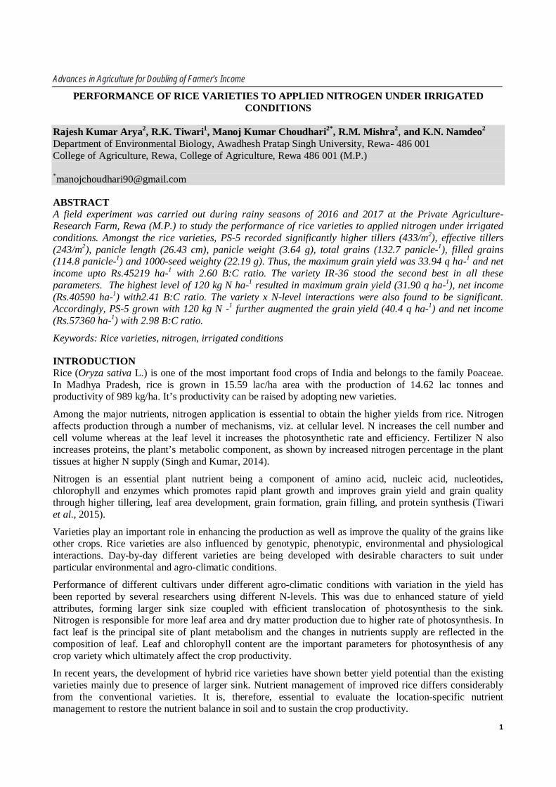
Crop+ Dairy+ Goat +poultry 50150 3500 6500 0 60150
Crop+ Dairy+ Goat +poultry + pigry 63200 0 2000 0 65200
Crop+ Dairy+ Fishries +Goat +poultry 51750 0 4000 0 55750
Table 2: Improvement of total net income (Rs) and natural resources S.N
Farming Systems
Holding size (ha)
Net income (Rs) Natural Resource improvement
Benchmark After diversification (First
year)
Second year
Third year
OC (%)
Before After 1st year
2nd year
3rd year
1 Crop + Dairy+
Poultry 0.72 50560 61310 80866 77,650 0.61 0.68 0.71 0.71
2 Crop +
Dairy+Goatry +Poultry
0.81 60150 78383 107800 100,900 0.59 0.63 0.74 0.75
3
Crop+ Dairy+ Goatry+ Poultry +
Pigry
0.80 65200 82575 1,22,275 1,30,850 0.62 0.69 0.76 0.77
4
Crop+ Dairy+ Fish +
Goatry+Poultry
0.82 55750 80705 114805 1,18,050 0.58 0.68 0.76 0.74
RESULTS 1. All modules have shown higher net return after intervention over farmer’s practice.
2. Crop module, livestock module and processing module gave additional return (25-35%) over before intervention or farmer practices.
3. The highest mean net income was obtained from farming system -crop+dairy+goat+pig+poultry after three year (Rs. 1, 30, 850 over benchmark Rs. 65200) followed by crop + dairy + fishery + goatry + poultry (Rs. 1,18, 050) over benchmark (Rs. 55750) for marginal farmers.
4. Farmers livelihood has improved over benchmark
RFERENCES Ansari, M.A., Prakash, N., Baishya, L.K., Punitha, P., Sharma, P.K., Yadav, J.S., Kabuei, G.P., and Ch,
K.L.L. (2014). Integrated Farming System: An ideal approach for developing more economically and environmentally sustainable farming system for the eastern Himalayan Region Indian J. Agric. Sci. 84, 356-362.
Chand, R., Prasanna, P.A.L. and Singh, A. (2011). Farm size and productivity: Understanding the strengths of smallholders and improving their livilihoods. Economic and Political Weekly 46, 10-14.
Singh, G. (2004). Farming systems options in sustainable management of national resources. In: Proceedings National Symposium on Alternative Farming Systems, held at PDCSR, Modipuram, 16–18 September, 2004, pp. 80-94.

Advances in Agriculture for Doubling of Farmer’s Income
18
COMPARATIVE PERFORMANCE OF DIFFERENT SEED BED CONFIGURATIONS IN SOYBEAN CULTIVATION IN MANDSAUR DISTRICT OF MADHYA PRADESH
Rajesh Gupta1, Akhilesh Singh2, Rupak Kumar3 and Ajeet Sarathe3*
1RVSKVV, KVK, Mandsaur- 458001 (MP) 2RVSKVV, Gwalior- 473551 (MP) 3Department of Agril. Engg., AKS University, Satna- 585001 (MP)
ABSTRACT The field trials were conducted during the three consecutive years Kharif 2016, Kharif 2017 and Kharif 2018 at farmer’s field in the adopted villages of Krishi Vigyan Kendra, Mandsaur to assess the effect of different seed bed configurations on growth characters and yield of soybean crop. The experiment consists of three seed bed configurations i.e., flat bed sowing by conventional seed drill (T1), ridge & furrow sowing by modified conventional seed drill (T2) and broad bed sowing by broad bed furrow seed drill (T3) with ten replications. The treatment T3 was found significantly superior in terms of plant population, plant height at flowering, number of root nodules per plant at flowering, number of pods per plant, number of branches per plant at harvest, grain yield, straw yield and harvest index as compared to treatments T1 and T2. The grain yield was found significantly higher in treatment T3 (16.74 q/ha) followed by treatment T2 (14.89 q/ha) and treatment T1 (12.14 q/ha). The treatment broad bed sowing by broad bed furrow seed drill (T3) recorded highest net return of 38635 Rs/ha with B:C ratio of 2.93:1 was found economically feasible as compared to field sown by modified (ridge & furrow) conventional seed drill (32160 Rs/ha, 2.61:1) and conventional seed drill (23007 Rs/ha, 2.a8:1) in Mandsaur district of Madhya Pradesh.
Keywords: Soybean, BBF, Grain yield, Net return, B:C ratio
INTRODUCTION Soybean (Glycine max. L.) is a major crop grown during the Kharif or monsoon season in the rainfed areas of central and peninsular India. Soybean is known as “Golden bean”, “Miracle crop” etc., because of its several uses. In India, the soybean crop presently covers an area of about 12 million hectares with a total production of about 14 million tonnes (Directorate of Economics and Statistics, 2016). The three largest soybean producing states are Madhya Pradesh, Maharashtra and Rajasthan. Soybean has emerged as a potential crop for changing the economic position of the farmers in India particularly in Madhya Pradesh. For improvement of agricultural productivity the package of improved implement, machines play important role, besides high yielding varieties, fertilizer, irrigation and plant protection practices. Mechanization of agriculture has assumed greater importance for increasing agricultural production and productivity by efficiently and effectively utilizing scarce resources and costly farm inputs improving timeliness factor, reducing labour cost and human drudgery etc. for soybean and wheat cropping system. Most of the farmers used seed drill for sowing of soybean on flat bed system, but due to improper drainage in the field, the yield of soybean reduced drastically.
Land treatments (raised sunken bed system, ridges and furrows, broad bed and furrows) increased in situ soil moisture conservation, minimized runoff, and soil erosion (Singh et al., 1999). Change over from growing crops in flat bed to ridge-furrow system of planting crops on broad bed alters the crop geometry and land configuration, offers more effective control over irrigation and drainage as well as their impacts on transport and transformations of nutrients, and rainwater management during the monsoon season. In Central India, majority of the area under soybean–wheat based cropping system is covered under vertisols and associated soils (Bhatnagar and Joshi, 1999). These soils are potentially productive, if managed properly in terms of overcoming soil, water and nutrient management constraints.

Advances in Agriculture for Doubling of Farmer’s Income
19
In recent years, broad bed system has proved to be one of the important components of low cost sustainable production system. This planting system facilitates mechanical weed control, increased water use efficiency, reduced crop lodging and has lower seed requirement (Sayre, 2000). Potential agronomic advantages of beds include improved soil structure due to reduced compaction through controlled trafficking, reduced water logging and timely machinery operations due to better surface drainage. Beds also create the opportunity for mechanical weed control and improved fertilizer placement (Singh et al., 2002). Jat and Singh (2003) reported higher biological yield and highest net and gross return from land configuration treatment as compared to conventional system. Presently, most of the farmers are being used seed drill for sowing of soybean on flat bed system, but the yield of soybean reduced drastically due to improper drainage in the field. Water logging adversely affects the growth of crop, primarily due to reduced oxygen supply to the roots. Therefore, to overcome the crop from excess moisture as well as moisture stress during crop growth period a field experiment was conducted at farmer’s fields to study the effect of different seed bed configurations on the growth characters and yield of soybean in Mandsaur district of Madhya Pradesh.
MATERIALS AND METHODS The study was carried out during during the three consecutive years Kharif 2016, Kharif 2017 and Kharif 2018 at farmer’s field in the adopted villages of Krishi Vigyan Kendra, Mandsaur namely, Daloda rail, Gurjar bardiya and Gogarpura to assess the effect of different seed bed conFig. urations on growth characters and yield of soybean crop. The experiment consists of three seed bed conFig. urations i.e., flat bed sowing by conventional seed drill (T1), ridge & furrow sowing by modified conventional seed drill (T2) and broad bed sowing by broad bed furrow seed dr ill (T3) with ten replications. The study area is situated in western part of Madhya Pradesh which falls under agro-climatic zone of Malwa plateau. Mandsaur belongs to sub-tropical climate having a mean temperature range of minimum 5 ºC and maximum 44 ºC in winter and summer, respectively. The topography of the experimental site was uniform and leveled. The soil is clayey in texture with 45 cm depth with pH 7.5 to 7.7, organic carbon 6.1 to 6.4 g/kg soil, EC 0.40 to 0.42 dS/m at the start of experiment. The area normally receives annual rainfall ranging from 750-800 mm per annum out of which about 90 per cent of is received between June and September.
A tractor drawn BBF seed drill developed by Indian Institute of Soybean Research (Formerly DSR), Indore, Madhya Pradesh was used for sowing of soybean crop in experimental plot under treatment T3 whereas conventional and modified (ridge & furrow) conventional seed drill was used under treatment T1 and T2, respectively. The dead furrows developed by broad bed furrow seed drill were useful to drain out excessive rainwater during heavy storms and for storing rainwater in furrows for enriching soil moisture through percolation in case of deficit rainfall. The recommended seed rate 80 kg/ha was used for sowing along with recommended package of practices including use of fertilizers and appropriate Rhizobium inoculation. The recommended dose of nutrient for soybean i.e., 20 kg N, 60 kg P2O5 and 20 kg K2O ha -1 was applied in all the treatments. Required plant protection measures were taken as and when found essential.
The observations on plant population, plant height at flowering, number of root nodules per plant at flowering, number of pods per plant, number of branches per plant at harvest, grain yield, straw yield and harvest index were recorded for all the treatments and analyzed statistically. The economics of the present study was also worked out for all three experimental years i.e., Kharif 2016, Kharif 2017 and Kharif 2018. The technique of representative sample was adopted for recording the observations on various morphological characters in soybean. At every observation, five plants from each treatment plot were randomly selected and tagged. The details of methodology adopted for recording the various observations are given in table 1.
RESULTS AND DISCUSSION The year wise (Kharif 2016, Kharif 2017 and Kharif 2018) and pooled data on parameters related to crop growth and yield as influenced by different seed bed configurations in soybean are presented in table 2. The statistical analysis showed that there was no significant difference (P≥0.05) on plant population and number

Advances in Agriculture for Doubling of Farmer’s Income
20
of branches per plant at harvest due to different treatments. The year wise and pooled mean data related to other crop growth and yield parameters were found higher in treatment T3 (broad bed sowing by broad bed furrow seed drill) as compared to in treatment T1 (flat bed sowing by conventional seed drill) and treatment T2 (ridge & furrow sowing by modified conventional seed drill). The plant height at flowering was found maximum in treatment T3 (45.69 cm) followed by treatment T2 (43.75 cm) and treatment T1 (41.93 cm). The increase in plant height was mainly due to better soil plant water relationship and soil physical condition in treatment T3. Similarly other crop growth and yield parameters viz., number of root nodules per plant at flowering, number of pods per plant, grain yield, straw yield and harvest index were significantly influenced by different land configuration at all the growth stages. The number of root nodules per plant at flowering, number of pods per plant, grain yield, straw yield and harvest index were recorded lower in treatment T1 than treatment T2 and treatment T3. The increase in root nodules in treatment T3 (21.07) by 21.21% than treatment T1 (22.69) and 9.57% than treatment T2 (25.07) may be due to better root development as treatment T3 and treatment T2 provided better physical condition of soil and lower penetration resistance to roots. Lupwayi et al. (1997) reported the 33% reduced nodules dry matter due to water logging condition. The broad bed planting also encouraged development of pods as treatment T3 (53.34) and treatment T2 (50.25) recorded higher number of pods per plant as compared to treatment T1 (47.14). The present findings are in close vicinity of Raut et al. (2000) and Jha et al. (2014).
Table 1: Details of methodology adopted for recording the observations S. No. Parameter Procedure followed
1. Plant population (no./m row length)
The plant population was counted from five randomly selected places for all the experimental plots
2. Plant height at flowering (cm)
The five plants were randomly tagged to count the plant height at flowering for all the experimental plots
3. Number of root nodules per plant at flowering
The five plants were dug up randomly from each plot and nodules were counted after its washing at flowering stage
4. Number of pods per plant The total number of pods of five plants was counted and average numbers of pods was calculated
5. Number of branches per plant at harvest
The five plants were randomly tagged to count the number of branches per plant for all the experimental plots
6. Harvest Index, HI (%) HI=[Economic yield (kg/ha)/Biological yield (kg/ha)] x100 where, Biological yield = Grain yield + Straw yield
7. Net return (Rs/ha) Net return (Rs/ha) = Gross return (Rs/ha)- Cost of cultivation (Rs/ha)
8. Benefit cost ratio (B:C) B:C = Gross return (Rs/ha)/Cost of cultivation (Rs/ha)
Table 2: Comparison of crop growth and yield parameters as influenced by different seed bed configurations in soybean

Advances in Agriculture for Doubling of Farmer’s Income
21
The grain yield and straw yield were found maximum in treatment T3 (16.74 q/ha and 34.87 q/ha respectively) followed by treatment T2 (14.89 q/ha and 31.71 q/ha respectively) and treatment T1 (12.14 q/ha and 26.47 q/ha, respectively). Superior yield with treatment T3 was mainly due to increased number of pods as the results of conserving more rainwater, nutrient and soil resources. Similar results of higher yields in altered land configuration over flat bed method were also reported by Autkar et al. (2006) and Selvaraju et al. (1999). The harvest index was also observed higher in treatment T3 (32.44) as compared to treatment T2 (31.96) treatment T1 (31.85).
The economics of the present study was worked out for all the experimental years i.e., Kharif 2016, Kharif 2017 and Kharif 2018 as well as for pooled mean data. The benefit cost ratio (B:C) and net return are the best indices to express the profitability of soybean cultivation which were calculated on the basis of cost of cultivation and gross return. From table 3, it is clear that the higher net return of 38635 Rs/ha with B:C ratio of 2.93 was recorded for soybean cultivation under treatment T3 followed by treatment T2 (32160 Rs/ha and 2.61) and treatment T1 (23007 Rs/ha and 2.18). Gupta et al. (2018) were also reported an increase in net return and B:C ratio of soybean cultivation due in altered land configuration over flat bed method.
Table 3: Comparison of economics parameters as influenced by different seed bed configurations in soybean
Parameter Treatment T1 Treatment T2 Treatment T3 Kharif 2016
Kharif 2017
Kharif 2018
Pooled Kharif 2016
Kharif 2017
Kharif 2018
Pooled Kharif 2016
Kharif 2017
Kharif 2018
Pooled
Cost of Cultivation
(Rs/ha)
19350 19450 19650 19483 19700 19900 20300 19967 19700 19900 20300 19967
Gross Return (Rs/ha)
42315 41860 43295 42490 52255 51485 52640 52127 58730 58205 58870 58602
Net Return (Rs/ha)
22965 22410 23645 23007 32555 31585 32340 32160 39030 38305 38570 38635
Benefit Cost Ratio
(B:C)
2.19 2.15 2.20 2.18 2.65 2.59 2.59 2.61 2.98 2.92 2.90 2.93
CONCLUSION It can be concluded that the practice of soybean cultivation on broad seed bed configurations was found superior in comparison with flat bed and ridge & furrow method of sowing. The results of the study indicated that the higher productivity (16.74 q/ha) with maximum net return (38635 Rs/ha) of soybean cultivation could be achieved by broad seed bed configurations as compared to flat bed and ridge & furrow method of sowing in Malwa region of Madhya Pradesh.
ACKNOWLEDGMENT With sincere respect and gratitude, we would like to thank Director, ATARI, (ICAR) Zone IX, Jabalpur and Director Extension Services, RVS Agriculture University, Gwalior for providing facilities, financial support and valuable guidance for the research work.
REFERENCES Autkar, K.S., Gawande, R.L., Vyas, J.S. and Ghodpage, R.M. (2006). Effect of land
configuration on yield and water use efficiency of soybean in vertisols of Vidarbha (M.S.). Ann. Pl. Physio. 20: 158-159.
Bhatnagar, P.S. and Joshi, O.P (1999). Soybean in cropping systems in India. Integrated Crop Management Series, FAO, Rome 3: 1-39.
Directorate of Economics and Statistics (DAC&FW, MoA&FW). (2016). Pocket Book of Agricultural, pp. 154.
Gupta, R., Kulmi, G.S., Basediya, A.L. and Jadav, M.L. (2018). Influence of furrow irrigated raised bed seed drill on growth characters and yield of soybean (Glycine max L.) in Mandsaur district of Madhya Pradesh, India. Plant Archives 18: 320-324.

Advances in Agriculture for Doubling of Farmer’s Income
22
Jha, A.K., Dwivedi, B.S., Shrivastava, A.K., Soni, M., Taniwaki, K., Kokuryu, T., Kitagawa, I., Tateishi, K., Tsuji, K. and Kobayashi, S. (2014). Effect of drainage, tillage and land configurations on root, nodules and yield of soybean in vertisols. Soybean Res. 12: 194-198.
Jat, L.N. and Singh, S.M. (2003). Varietal suitability, productivity and profitability of wheat (Triticum species) intercrops and relay cropping under furrow irrigated raised bed system. Indian J. Agric. Sci. 73: 187-190.
Lupwayi, N.Z., Haque, I. and Holl, F.B. (1997). Strain specific response of Trifolium semipilosum to inoculation with Rhizobium and the significance of water logging in vertisols. J. Agric. Sci. 129: 439-446.
Raut, V.M., Taware, S.P., Halvankar, G.B. and Varghese, P. (2000). Comparison of different sowing methods in soybean. J. Maharashtra Agril. Univ. 25: 218-219.
Sayre, K. (2000). Saving water and increasing sustainability with bed planting. Outlook, 1: 5.
Selvaraju, R., Subbian, P., Balasubramanian, A. and Lal, R. (1999). Land configuration and soil nutrient management options for sustainable crop production on alfisols and vertisols of southern peninsular India. Soil Tillage Res. 52: 203-216.
Singh, P., Alagarswamy, G., Pathak, P., Wani, S.P., Hoogenboom, G and Virmani, S.M. (1999). Soybean-chickpea rotation on Vertic Inceptisol: I. Effect of soil depth and landform on light interception, water balance and crop yields. Field Crops Res., 63: 211-224. II. Long-term simulation of water balance and crop yields. Field Crops Res. 63: 225-236.
Singh, S., Yadav, A., Malik, R.K., and Singh, H. (2002). Furrow irrigated raised bed planting system: a resource conservation technology for increasing wheat productivity in rice-wheat sequence. In: Malik, R.K. et al. (Ed.), Herbicide resistance management and zero tillage in rice-wheat cropping system. Proc. Int. Workshop, Hisar, India, 4-6 March 2002, CCS HAU Hissar, India, pp. 198-200.

Advances in Agriculture for Doubling of Farmer’s Income
23
ASSESSMENT OF CROP WATER REQUIREMENT FOR VEGETABLE CROP OVER UTTAR PRADESH USING CROPWAT MODEL
Shashank Kumar1, Lakshmi Prasanna Aggile1*, Himani Bisht2 and Shweta Gautam1 1Department of Environmental Sciences and Natural Resource Management, SHUATS, Prayagraj, Uttar Pradesh, India 2Water Technology Centre, ICAR-IARI, New Delhi, India
ABSTRACT Water scarcity becomes a major intimidation to crop production. There are a lot of changes in climate that affects on hydrological process. It will fall directly on agricultural production and productivity. Mostly vegetables are grown under irrigation and very quickly suffered from drought. Supplemental irrigation was essential for good yields. In this manner present study was conducted on water requirements on vegetables (potato, pea and cabbage) over Uttar Pradesh with help of Cropwat software using the weather data of minimum temperature, maximum temperature and rainfall for the period 1980-2014. The analysis was performed in two date of sowing 15th October and 15th November. The seasonal crop water requirement (ETc) and irrigation water requirement (IWR) of potato varied between 271 mm (Bijnor) to 409.1 mm (Lalitpur) and 218 to 360.9 mm respectively for 1st date of sowing. While for 2nd date of sowing ETc and IWR ranged between 287.3 mm (Bijnor) to 439.1 mm (Lalitpur, Jhansi & some parts of Mahoba) and 219.2 mm to 392.7 mm respectively. The ETc and IWR of Pea varied between 206.6 mm to 303.6 271 mm and 184.6 mm to 274.1 mm respectively for 1st date of sowing. While for 2nd date of sowing ETc and IWR ranged between 181.5 mm to 279.7 mm and 145.6 mm to 246.6 mm respectively. The ETc and IWR of Cabbage varied between 388.1 mm to 577.4 mm and 309.5 mm to 519.2 mm respectively for 1st date of sowing. While for 2nd date of sowing ETc and IWR ranged between 453.3 mm to 655.9 mm and 368.4 mm to 604.1 mm respectively. The experimental analysis revealed that early date of sowing (15th October) required less ETc and IWR as compared to other date of sowing. Further to observe the effect of long term climate change (year 2020, 2050 and 2080) on ETc and IWR of Potato were estimated using IPCC AR5 data with RCP 4.5 scenario. Results revealed that with the time ETc and IWR has found to be increased. This study is capable for strategic planning in irrigation management and scheduling in the view of water saving technologies.
Keywords: Climate change, ETc, Cropwat, Arc GIS, Potato, Pea, Cabbage
INTRODUCTION Water Scarcity is becoming a major problem in worldwide due to increasing demand in agriculture and other sectors. It is an essential input for crop production so planning and delivery of this precious resource is necessary. Scarcity and growing competition for fresh water resource will reduce its availability for irrigation. Agriculture is largest consumer of water in India and most efficient use of water in agriculture needs to be a top most priority (Anshu et al., 2017). Considering the current water resources problems and rapid increase in its demand, proper planning and management of water resources is important to increase agricultural production (Bajirao et al., 2017).
Vegetables are being cultivated mainly in Rabi season with irrigation. The water requirements of vegetable crops are less. But unknowingly the farmers are applying more water. Actual water shortages are observed in many countries particularly in India. It is important that the water requirements of crops are known at different management levels within the irrigated area to accomplish effective irrigation management. The main objective of irrigation is to apply water to soil to meet crop evapotranspiration requirement when rainfall is insufficient to raise crop till harvesting. Potatoes have become a staple food in many parts of the world. Potatoes are the world's fourth-largest food crop. Uttar Pradesh is the major crop producer in Potato (2017-18), area sown is 614.8 Thousand Ha. Potato may be more sensitive to water stress than any other crops, because it has a sparse root system that is concentrated in the upper 30 cm soil layer. Potato is grown throughout the world and plays a vital role in human nutrition and food economy. Cabbage is one of the most important vegetables grown worldwide (Rokayya et al., 2013) The Food and Agriculture Organization of the

Advances in Agriculture for Doubling of Farmer’s Income
24
United Nations (FAO) reported that world production of cabbage and other brassicas for 2014 was 71.8 million metric tonnes. On average twice week irrigation scheduling and 2.57 - 5.81 mm /day of crop water requirement is more visible for cabbage production. In India pea is being grown in rainfed conditions and is subjected to unpredictable drought during crop season. But pea is a crop which responses favourably well to irrigation. The water relations of pea have often been considered in relation to three successive developmental stages: from planting until the start of flowering; during flowering; and the period of pod and seed growth and maturation. Availability of water, whether as rain or from irrigation, has been a major factor influencing the distribution and yield of pea. Consumptive water use (CWU) of these crops varies with species, climatic and soil conditions, and with the growth period. It amounts to between 350 and 500 mm per year (FAO, 1979).
MATERIALS & METHODOLOGY Experimental Site: Uttar Pradesh is situated in Northern India between 26.8467° N Latitude and 80.9462° E Longitudes. The state has 75 districts with a total area of 243,290 square kilometres. Uttar Pradesh is India's fourth-largest state in terms of land area. The average annual rainfall varies from 50-110 cm in Uttar Pradesh. South West Monsoon is very moderate Uttar Pradesh and it rains very heavily in short spells. The Western disturbance brings fair amount of rainfall.
Data Collection: The data used in this study are mainly meteorological data, including precipitation, minimum air temperature and maximum air temperature from 1980 to 2014 in 24 meteorological stations. Arc/Info grid spline method is used to interpolate the point climate data into the 1km×1km grid data.
Cropwat 8.0 Details: CROPWAT is a decision support system developed by the land and water development division of FAO. It is used to estimate (a) Reference evapotranspiration (b) Crop water requirements (c) Crop Irrigation requirements in order to develop irrigation schedules under various management conditions (FAO, 1992). In the present study Cropwat software was used for calculating crop water requirement over Uttar Pradesh for wheat crop at different date of sowing with changing climate. ETc is derived by estimating the ETo. It was calculated using the equation:
Where, ETo = reference evapotranspiration (mm per day), Ra = net radiation at the crop surface (MJ/m² per day), G = soil heat flux density (MH/m² per day), T = mean daily air temperature at 2m height (°c), u2 = wind speed at 2m height (m/s), es = saturation vapor pressure (kPa), ea = Actual vapor pressure (kPa), es – ea = saturation vapor pressure deficit (kPa), γ = psychometric constant, Δ = slope vapour pressure curve [kPa °C-1].

Advances in Agriculture for Doubling of Farmer’s Income
25
ESTIMATION OF CROP WATER REQUIREMENT (ETC) Crop Water Requirement is the amount of water needed to meet the water loss through Evapotranspiration. Estimation of the crop water requirement is derived from crop evapotranspiration (crop water use), which is the product of the reference evapotranspiration (ETo) and the crop coefficient (Kc). The reference evapotranspiration (ETo) is estimated based on the FAO Penman-Monteith method, using climatic data (FAO, 1998).
ETc = ETo × Kc
Where, ETc = Actual evapotranspiration by the crop (mm/day), ETo= Reference crop evapotranspiration (mm/day) and K C = Crop coefficient at a certain growth stage.
ESTIMATION OF IRRIGATION WATER REQUIREMENT (IWR) Irrigation requirement is the total quantity of water applied to the land surface in supplement to the water supplied through rainfall and soil profile to meet the water needs of crops for optimum growth. Based on the effective rainfall data in the study area, irrigation water requirements can be calculated from the difference between effective rainfall and the total water requirement.
IR= ETc – ER
Table 1: Crop coefficients of potato, pea and cabbage Crop Crop Coefficients
Initial (Kc1) Development (Kc2) Late Season (Kc3) Potato 0.5 1.15 0.75
Cabbage 0.7 1.05 0.95 Pea 0.5 1.15 1.10
4. EXPERIMENTAL FINDINGS 4.1 Reference Evapotranspiration Evapotranspiration can be calculated with proper weather data available about selected years. Crop evapotranspiration over 30 years is in more areas, over Uttar Pradesh. Reference evapotranspiration (ETo) is an important agrometeorological parameter for climatological and hydrological studies, as well as for irrigation planning and management. The FAO Penman-Monteith (FAO PM) method has been considered as a universal standard to estimate ETo (Allen et al., 1989).
Evapotranspiration started to decreases in the months of December followed to January and February, it is due to start of lowest temperature in the months with low relative humidity. In line with the research Patel estimated ETo in Ludhiana from 1970-2012 increased during the March-October, reached maximum value of 205.2 mm/month at June and declined during November and December months.
Fig. 1. Thematic map of reference evapotranspiration (ETo) during 1980-2014

Advances in Agriculture for Doubling of Farmer’s Income
26
From thematic map (Fig. 1) of annual ETo over UP clearly revealed that the annual ETo was found maximum in the lower belt of the state as Jhansi, Mahoba, Banda, Lalitpur etc districts ranged between 1648.3 to 1726.3 mm. The lowest value of Eto was observed in Muzaffarnagar and Bijnor ranged between 1335.9 to 1414.0mm. Average peak monthly ETo was estimated in the month of May and April, respectively due to high temperature during the summer month. Average minimum monthly ETo was observed in the month of January and December, respectively due to winter months.
Crop Evapotranspiration (ETc) and Irrigation water requirement (IWR) for Potato, Pea & Cabbage at different environmental conditions over Uttar Pradesh: Potato (Solanum tubrosum L.), pea (Pisum sativum L.) and cabbage (Brassica oleracea L. var. capitata) is most important vegetables crops over Uttar Pradesh. Climate data, rainfall data, crop data, cropping pattern data and soil data were fed to the Cropwat 8.0 model for the estimating the water requirements for potato, pea and cabbage during period 1980-2014 at two date of sowing. The estimated water requirements for two different dates of sowing for potato, pea & cabbage crop were presented as thematic representation (Fig. 2).
For potato crop the average ETc was found minimum at early sowing (15 Oct.) as compare to delay sowing (15 Nov.). The water requirement of early sown starts rising from mid-November during tuber initiation stage of the crop. The water requirement remains high throughout December. It is interesting to note that, this period coincides with the tuber formation stage of the crop, which is critical stage for potato regarding water. The reduction of water demand at the first half of the January can be explained by lowest average temperature prevailing during this period. However, the water requirement again increases at maturity stage during February. In case of late sown, the water requirement shows an increasing trend during the tuber formation stage extending approximately from January to February. Being a late sown (potato2) crop, late sown exposed to higher temperature during later part of its growing period. As a result, the water demand remains high as compared to early sown. The total water requirement of potato sown at an early date is vary 271 mm to 409 mm and that of sown at late date is 287.3 mm to 439 mm. More over irrigation water requirement at an early date is vary 218.3 mm to 360.8 mm and that of sown at late date is 219.2 mm to 392.6 mm. Overall Bijnor district consume less water requirement, it may be due to the geographical location as it comes close to hill state. While Lalitpur and Jhansi districts consumes more water requirement.
Pea crop which responses favorably to irrigation. Even one irrigation, applied at growth or development stage, gives quite good yield of pea. Etc was found minimum in Bijnor district ranged between 206.6 to 226 mm while maximum Etc was found in Lalitpur and Jhansi. While late sowing, consumes 181.5 to 201.1 mm while maximum ranged between 260.5 to 279.6 mm. The irrigation water requirement showed maximum value in Bijnor district at 184.6 to 202.5 mm at 1st DOS, while maximum IWR was found in Lalitpur and Jhansi. At 2nd day of sowing, the IWR was found minimum in Bijnor district ranged between 145.6 to 165.8 mm while maximum IWR was found in Lalitpur and Jhansi ranged between 226.4 to 246.5 mm (Fig. 2).
Estimation of water requirements for cabbage would help farmers avoid water wasting and financial loss related to the traditional techniques. The Etc & IWR was found minimum in Bijnor district ranged between 388.1 to 426 mm and 309.5 to 351.4 mm, respectively. While maximum Etc was found in Lalitpur and Jhansi. Late sowing consumes minimum in Bijnor district ranged between 453.3 to 498.5 mm and 368.4 to 415.6 mm for ETc and IWR, maximum was found in Lalitpur and Jhansi ranged between 615.3 to 655.8 mm and 556.9 to 604 mm.
a. Potato

Advances in Agriculture for Doubling of Farmer’s Income
27
b. Pea
c. Cabbage
Fig. 2. ETc & IWR for potato, pea and cabbage for 1st date of sowing over UP
Delay in sowing (2nd DOS) represents large amount of ETc as compare early sowing. Therefore, it was observed that 1st DOS gave best result for planning of irrigation water for potato and cabbage. In case of pea 2nd date of sowing represents less amount of crop water requirement as compare to 1st date of sowing.
Babu et al. (2014) was found similar findings as estimation of crop water requirement of Anantapur region for the groundnut kharif and rabi crop as 591.3 mm and 443.3 mm, respectively and for vegetables, cotton, rice, pulses and maize as 594.1 mm, 878.6 mm, 1110.6 mm, 659.9 mm and 679.3 mm, respectively through Cropwat software.
Impact of climate change on crop water requirement Climate is a one of the important factor determining the crop water requirements. Increasing of meteorological factors may have negative effect on water requirements, for better management of agricultural productions, it is important to understand ETc and possible effects of climate change in future. ETc can be predicted by several methods. The crop water requirement with changing climate can also predicted by CROPWAT model. To analyses the effect of climate change the climatic scenarios for the year

Advances in Agriculture for Doubling of Farmer’s Income
28
2050 & 2080 were obtained from the Marksim DSSAT IPCC AR5 were presented in table 2. MarkSim is a weather generator that uses 720 classes of weather, worldwide. This constitutes 'stochastic downscaling' as it fits a Markov model to the GCM output and uses it to generate weather data for the site indicated. The model estimates indicate an increase in future irrigation as compared to the base period. In this view, it is necessary to find the solution for improving current water conditions for summer-autumn crops to acclimatize for the changes of precipitation and temperature in the future and also minimise the water scarcity by shifting the planting dates.
Table 2: Crop Water Requirement (ETc) at different date of sowing (15 Oct. & 15 Nov.) for potato, pea & cabbage (2050 & 2080)
Station Potato Pea Cabbage 2050 2080 2050 2080 2050 2080
I II I II I II I II I II I II Ambedkar Nagar
419.1 443 421.7 445 311.4 280.6 314 282.8 582 649.1 592 660.4
Aurariya 388.5 417.8 398.3 429.8 292.8 263 297.4 267 554.8 642.4 570.2 661.4 Bahraich 363.1 398 368.6 405.1 270.4 249.4 275.3 252.4 523 616.2 533.1 629.8 Balampur 363.6 339.9 371.6 409.6 268.5 250.8 274.2 256.4 522.6 612.5 535 626.9 Banda 396.4 436.3 404.7 446.4 293.1 271.9 298.6 277.8 570.8 663.1 583.5 679 Bareily 351.2 378 361.1 388.9 264.2 238.4 271.5 245.3 502.8 586.7 516.9 603.7 Bijnor 332.4 355.6 336.7 360 252 223.6 256.4 225.7 476.5 557.2 483.5 565.9 Etah 376.2 400.3 386.9 412.8 286.2 252.5 294 259.8 536.1 617.3 552.6 638.3 Farukhabad 374.8 404.1 385.5 415.9 283.1 253.5 291 260.9 537.3 625.7 552.5 644.5 Gautambudh Nagar
356.8 375.9 265.8 385.6 272.4 240.1 279.5 246 504.5 579.8 517.7 596.1
Ghazipur 374.3 410.7 381.8 420.7 278.5 257.3 283.4 262.6 538.5 626.8 551.1 643.8 Gorakhpur 357.6 392.2 365.1 401.5 266 246.5 271.3 251.9 515.6 602.9 527.4 618.2 Jaunpur 383.4 418.9 390.4 428.5 284.4 264 288.6 269.2 549.2 642.9 560.8 655.1 Jhansi 406.7 438.8 418 452.2 301.3 279.6 309 287.5 575 655.5 591.8 675.4 Kaushambi 398.3 432.1 404.8 441.1 294.6 274.6 299 279.8 565.6 653.9 575.9 667.6 Kheri 345.6 384.8 351.5 392.7 253.7 238.2 258.5 241.5 503.3 600.4 514.2 615.1 Lalitpur 406.3 442.9 415.8 454.1 297.1 282.1 303.6 289.1 575.4 656.7 589.2 673.1 Maharajganj 358 396.3 364.4 404.3 263.6 247.6 268.3 252 517 604.1 527.4 617.3 Mahoba 404.9 442.2 414.6 453.5 299.4 277.9 306.1 284.9 578 666.9 592.2 684 Mathura 278 400.8 386.2 409.8 286.3 254.5 293.6 258.2 536.2 614.3 549.3 631 Moradabad 338.9 363.4 347.1 372.6 255.8 229.2 261.8 234.8 485.3 567.3 497.1 581.6 Sitapur 350.1 392.1 359.5 402.4 255.3 241.6 262.5 248.2 511.8 610.9 525.2 627.1 Sultanpur 371.5 405.4 379.7 415.6 276.4 254.7 281.8 260.8 533.4 623.2 545.7 641.4 Unnao 381.8 410.9 391.2 422.5 286.6 260.2 293 266.7 544 629.3 558.7 647.1
Table 3: Irrigation Water Requirement (IWR) at different date of sowing (15 Oct. & 15 Nov.) for potato, pea & cabbage (2050 & 2080)
Station Potato Pea Cabbage 2050 2080 2050 2080 2050 2080
I II I II I II I II I II I II Ambedkar Nagar 408.8 436.7 410.5 439.5 301.7 275.9 303.3 277.9 570.2 641.4 579.2 651.7 Aurariya 320.5 375.1 326.3 384.1 241.6 230 244.1 231.8 476.3 594.4 482.2 614.3 Bahraich 294.4 349.7 291.1 350.9 227.5 217.1 230.7 215.1 442 560.2 447.5 567.9 Balampur 307.3 363.1 310.9 366.9 229.8 227.1 234.1 227.4 454.7 566.3 462.5 574.8 Banda 335.7 393 338.3 399.3 250 240.7 251.4 243.7 497.9 618.3 504 630.3 Bareily 282.4 329.6 287.8 336.6 219.1 209.3 224.7 213.8 418.3 531.8 427.9 544.9 Bijnor 253.2 286.8 255.2 286.7 205.2 177.9 209.3 176.8 381.3 478.4 384.6 482.2 Etah 322.4 362.3 329.5 372.7 247.7 229.5 253.6 235.5 468.7 576.5 481.2 595.7 Farukhabad 300 355.2 307.2 363.4 226.4 217.9 233.1 222.8 447.4 574.8 458.6 590 Gautambudhnagar 305.7 337.6 309.7 343.8 237 213.5 240.4 216.6 443.5 536.1 451.2 549.1 Ghazipur 326 375.6 324.6 378.4 248.7 234.8 246.7 233 479.9 585.4 483.1 595.4

Advances in Agriculture for Doubling of Farmer’s Income
29
Gorakhpur 295.3 351.9 299.7 356.1 224 221.9 228.9 222.1 440.1 552.8 448.7 563.4 Jaunpur 337.1 385.1 336.4 388.8 254.1 242.2 252.6 241.2 498 599.1 502 605.8 Jhansi 358.3 405.4 363.5 414.9 268.4 256.1 271.2 261.1 520.7 617.3 530.7 633.2 Kaushambi 350.6 393.2 349.5 396.7 264 250.2 262.4 250.5 507.9 608 509.7 616.4 Kheri 273.6 332.6 275.7 335.4 205.2 204.2 209.5 204.1 411.8 545.2 418.6 554.6 Lalitpur 344.6 397.2 347.9 404.7 255.1 244.8 256.2 249.2 509.5 601.3 516.4 613.4 Maharajganj 296.8 360.2 301.3 363.7 219.5 223.6 225.2 223.9 441.5 557 449.4 566 Mahoba 355.7 403.8 358.9 410.9 270.1 248.6 271.7 252.5 522.8 628.1 529.6 640.9 Mathura 341 373.7 344 378.7 260.7 238.5 264 239.7 489.7 584.2 497.2 596.9 Moradabad 287.4 311 276.9 315.5 218.4 198.4 220.8 196.6 412.9 490.5 411.5 518.6 Sitapur 280.9 342.4 286.4 348.2 206.1 209.9 212.5 213 421.3 556.6 430.6 568.4 Sultanpur 317 370.3 318.7 374.9 238.9 231.3 240.2 231.8 474.1 576.9 479.9 589.6 Unnao 310.2 362.2 314.8 369.8 236.5 222.5 240.6 225.7 462.4 579.5 471.9 593.2
CONCLUSION Estimation of water requirements would help farmers avoid water wasting and financial loss related to the traditional techniques. Improved water resources management would promote efficient agricultural production and environmental sustainability. The late planting date requires a little more irrigation water for the whole season compared to the other planting date. Simulation results showed that crop water requirement decreased significantly after planting date is late shifted by 15 days in case of Pea crop and increased in case of Potato and Cabbage. The outcome of this study are capable for planners of water resources for future planning and helps to save water in satisfying crop water requirement and it can be used as a guide by the farmers for selecting the amount and frequency of irrigation for the crops studied under the consideration.
REFERENCES Anshu, G., Nayak, T.R., Singh, R.M. and Singh, A. (2017). Estimation of crop water requirement using
Cropwat 8.0 model for Bina command, Madhya Pradesh. Indian Journal of Ecology, 44, 71-76.
Babu, R.V., Kumar, G.J., Raja, K.N., and Bhaskara, R. (2014). Estimation of water requirement for different crops using CROPWAT model in Anantapur region. Asian J. Environ. Sci. 9, 75-79.
Bajirao, T.S. and Harish, W.A. (2017). Estimation of reference evapotranspiration for Parbhani district. Internat. J. Agric. Engg. 10, 51-54.
Doorenbos, J. and Pruitt, W.O. (1979). Guidelines for prediction crop water reqirment by. FAO Irrigation and Drainage, Paper No. 24.
Doorenbos, J. and Kasssam, A.H. (1979). Yield response to water. FAO Irrigation and Drainage, Paper No. 33.
Smith, M. (1992). CROPWAT, a computer program for irrigation planning and management. FAO Irrigation and Drainage, Paper No. 26.
Allen, R.G., Pereira, L.S., Raes, D. and Smith, M. (1998). Crop evapotranspiration. Guidelines for computing crop water requirements. FAO Irrigation and Drainage, Paper No. 56.
Rokayya, S., Chun, J.L., Zhao, Y., Ying, L. and Chang, H.S. (2013). Cabbage (Brassica oleracea L. var. capitata) phytochemical with antioxidant and antiinflammatory potential. Asian Pac. J. Cancer Prev. 14, 6657-6662.

Advances in Agriculture for Doubling of Farmer’s Income
30
MODEL DEVELOPMENT FOR YIELD FORECASTING THROUGH PRINCIPAL COMPONENT ANALYSIS AND STEPWISE REGRESSION ANALYSIS FOR PIGEON PEA CROP ON
CHHATTISGARH PLAIN ZONE
K.K. Pandey*, Gaind Lal, Bhashkar and Yogesh Chelak Department of Agril Statistics, Indira Gandhi Agriculture University, Raipur (C.G.)
ABSTRACT Agriculture is backbone of Indian economy. Economic survey 2014-15, by the CSO, the share of agriculture in total GDP is 18 per cent in 2013-14. The Kharif crops data released by the Directorate of Economics and Statistics recently indicates that India ranks 1st in area and production in the world with 80% and 67% of world's acreage and production. The state-wise mandi arrivals of pigeon pea during 2013-14 to 2016-17 therefore needs to do research to study weather situation and effect on crop production. Crop yield forecast provided useful information to farmers, Present study of model development for PCA and SRA on pigeon pea yield at Chhattisgarh Plain Zone on the basis of weather variables. Meteorological weekly data for pigeon pea crop, Model are fitted with PCA and SRA Respectively 2 Principal Components (PC1 and PC2) and Time trend (T). Models are highly significant and R2 value 69% for Pigeon pea for CG plain Zone is also significant at 0.1% level of significance And SRA Model the value of R2 for the model on Zone Level is 78% and 2 (Q121 and Z41) variable entered into models for Pigeonpea crop. The Both models have been also found highly significant.
Keywords: Pigeon pea, Coefficient of determination, Principal Component Analysis (PCA), Stepwise Regression Analysis (SRA)
INTRODUCTION Forecast of the crop production at suitable stages of crop period before the harvest are vital for rural economy. On the other hand, forecasts of crop yields are important for advance planning formulation and its implementation. Forecasting is also vital for crop procurement, distribution, price structure and import export decisions etc. These are useful to farmers to decide in advance their future prospects and course of action. Thus, reliable and timely pre-harvest forecasting of crop yield is very important. To meet such needs, crop forecasts under the prevalent system in India are being issued by the Directorate of Economics and Statistics, Ministry of Agriculture, New Delhi. The final estimates based on objective crop-cutting experiments are of limited utility as those become available quite later after the crop harvest. The statistical techniques employed for forecasting purposes should be able to provide objective, consistent and comprehensible forecasts of crop yield with reasonable precisions well in advance before the harvest. Several studies have been carried out to forecast crop yield using weather parameters etc.
These are useful to farmers to decide in advance their future prospects and possible course of action. Thus, reliable and timely pre-harvest forecasting of crop yield is very important. In statistical model approach, one or several variables (representing weather or climate) are related to crop responses such as yield and yield contributing characters. Therefore, there is a need to develop area specific forecasting models based on time series data to help the policy makers for taking effective decisions to counter adverse situations in food production. The forecasting of crop yield may be done by using three major objective methods (i) biometrical characteristics (ii) weather variables and (iii) agricultural inputs (Agrawal et al., 2001).
MATERIALS AND METHODS The principal component analysis has been also taken for the development of forecasting model. Time series data on yield for 25 years (1990-91 to 2014-15) for 4 districts, Seventeen years for 5 districts has been procured from Directorate of Agricultural, Govt. of Chhattisgarh. The weekly meteorological data (1990-91 to 2014-15) procured from IGKV, Raipur for pigeon pea crop period data. This procedure is based on the method given by Agrawal et al. (1986) for developing forecast model using weather indices. In this procedure the entire 17 weeks data (w = 1, 2,…17) was taken for pigeonpea crop.

Advances in Agriculture for Doubling of Farmer’s Income
31
Let m denotes the week (w = 1,2,…m) at which pre-harvest forecast of crop-yield need to be released. Using the weekly data on m weeks of p weather variables (p= 7 here), new weather variables and interaction components have been generated with respect to each weather variable. Forecast model has been developed considering all generated variables simultaneously including time trend (T).
Model – I : Y a bij z© ij
j 0
2
i1
p
bii © jj 0
2
ii © 1©
p
Qii © j CT
Where
Zij = riw
j
w1
m
Xiww1
m
riwj
and Qii ©,j
© rii ©,wj Xiw
w1
m
Xi ©w rii © ,wj
w1
m
Xiw is the value of the ith weather variable in wth week, riw/rii’w is correlation coefficient of yield adjusted for trend effect with ith weather variable/product of ith and i’th weather variable in wth week.
PCA is a multivariate technique for data reduction. It is a mathematical function, which does not require user to specify the statistical model or assumption about distribution of original variables (Anderson et al., 1984).
Let Xij be the value of jth biometrical character (j= 1, 2,...p) corresponding to ith varieties of experiment ( i= 1, 2,...n). The PCA for xij’s will be carried out. Let PC1, PC2, ....PCK be first K (K< P) principal components explaining variability about more than 70 to 90 per cent of the total variation in xij’s. Using these K principal components as regressor variables and varieties yield (yi) as regress and, the following linear multiple regression model for pre-harvest forecast of crop yield has been proposed.
Yi =β0 +β1 PC1i +β2 PC2i +...+βk PCki +ei , i= 1, 2, ....n.
Where Yi is the crop yield of the ith plot; β0, β1, β2 βk are model parameters and ei is error term assumed to follow independently normal distribution with mean 0 and variance σ2. The aforesaid model is fitted with the data by least square technique.
Measures for validation and comparison of the models Two procedures have been used for the comparison and the validation of the developed models. These procedures are given bellow.
Coefficient of determination (R2) and (R2adj)
The models were validated on the basis of (R2) and (R2adj) which can be computed from the formula given
by Drapper and Smith (1988).
Adjusted R2 is given by the following formula
Radj
2 1ssres n p sst n 1

Advances in Agriculture for Doubling of Farmer’s Income
32
where ssres/(n-p) is the residual mean square and sst/(n-1) is the total mean square. The total mean square is constant regardless of how many variables are in the model. On adding a regressed in the model Adjusted R2 increases only if the addition of the regressed reduces the residual mean square. It also penalizes for adding terms that are not helpful, so it is very important in evaluating and comparing the regression models.
Percent Deviation The formulae for computation of percent deviation of forecast yield from actual yield are given by Azfar et al. (2015) and Yadav and Sisodia (2015). This measures the deviation (in percentage) of forecast from the actual yield data. The formula for calculating the percent deviation of forecast is given below:
RESULTS AND DISCUSSION Model-1 developed throw PCA are two regressed variables have been entered in the model finally, which is given below:
Y= -60.02-2244.8PC1-4493.58PC2-22.50T
Table 1: Pre-harvest Forecast Model through PCA for CG Plain on Pigeon pea. Variables Coefficient Standard error P-Value Significance (R2) R2 (Adj )
Intercept -60.02 457.6254 0.001
0.69***
PC1 -2244.8+ 1169.402 0.06 PC2 -4493.58* 1903.943 0.02
T -22.50*** 4.60818 0.001 ***P<0.001, **P<0.01,*P<0.05, +P<0.1
The results given in Table 1.1 that all variables (PC1, PC2 and T), except PC1 fitted in the model have been found to be significant at 0.01, probability level of significance. The coefficient of determination adjusted (R2) has been found to be 69%, which is significant at 0.01% level.
Table 2: Validation of the model through PCA for PCA for CG Plain on Pigeon pea Year Actual rice yield(q/ha) Predicted rice yield(q/ha) Percent deviation 2010 384.67 323.1569 15.99 2011 416.22 397.9641 4.39 2012 546.11 310.4661 43.15 2013 481.62 544.3523 -13.02 2014 567.10 367.8191 35.14
**P<0.01, *P<0.05, +P<0.1
It can be observed from the results of the table 2 that the model is best fit and it has high power to pre-harvest forecast of pigeon pea yield. It means model is very reliable for forecasting at CG Plain.
Fig. 1 also shows the comparison between actual and predicted yields on the basis of 3 years data, almost same indication in results as well as graph.
Fig. 1. Comparison between actual and predicted yield on pigeon pea for PCA
Model 2- Y= 2866.11-5.63 Q121+19.95 Z41

Advances in Agriculture for Doubling of Farmer’s Income
33
Table 3: Pre-harvest Forecast Model through SRA for CG Plain on pigeon pea Variables Coefficient Standard error P-Value Significance R2 (Constant) 2866.11 673.037
0.0001
0.78***
Q121 -5.63*** .904 0.0001 Z41 19.95*** 4.879 0.0001
The results given in table 3 that all variables Q121, Z41, except T fitted in the model have been found to be significant at 0.01, probability level of significance. The coefficient of determination adjusted (R2) has been found to be 78%, which is significant at 0.01% level
Table 4: Validation of the model through SRA for CG Plain on pigeon pea Year Actual yield (q/ha) Predicted yield (q/ha) Per cent deviation 2010 384.67 314.2716 18.30 2011 416.22 338.7239 18.62 2012 546.11 419.0671 23.26 2013 481.62 648.9797 -34.75 2014 567.10 468.727 17.35
Fig. 2. Comparison between actual and predicted yield on Pigeon pea for SRA
REFERENCES Anderson, T.W. (1984). An introduction to multivariate statistical analysis. John Wiley & Sons, New
York.
Azfar M., Sisodia, B.V.S., Rai, V.N. and Devi, M. (2015). Pre-harvest forecasting models for rapeseed and mustard yield using principle component analysis of weather variable. Mausam, 761-766.
Agrawal, R., Jain, R.C. and Jha, M.P. (1986). Models for studying rice crop weather relationship. Mausam 37, 67-70.
Draper, N.R. and Smith, H. (1988). Applied regression analysis. 3rd edition, John Wiley & Sons Inc.
Agrawal, R., Jain, R.C. and Mehta, S.C. (2001). Yield forecast based on weather variables and agricultural input on agrioclimatic zone basis. Ind. J. Agric. Sci. 71, 487-90.
Pandey, K.K., Rai, V.N., Sisodia, B.V.S., Bharti, A.K. and Gairola, K.C. (2013). Pre -harvest forecast models based on weather variable and weather indices for eastern U.P. Advances in Bioresearch 4, 118- 122.
Pandey, K.K., Rai, V.N., Sisodia, B.V.S. and Singh, S.K. (2015). Effect of weather variables on rice crop in eastern Uttar Pradesh, India. Plant archives, 15, 575-579.
Kumar, N., Pisal, R.R., Shukla, S.P. and Pandey, K.K. (2016). Crop yield forecasting of paddy and sugarcane through modified hendrick and scholl technique for south Gujarat. Mausam, 67, 405-410.

Advances in Agriculture for Doubling of Farmer’s Income
34
Pandey, K.K., Maurya, D., Gupta, G. and Mishra, S.V. (2016). Yield forecasting models based on weather parameters for eastern U.P. Vegetos, 29, 1-3.
Pandey, K.K., Rai, V.N., Sisodia, B.V.S., Pandey, R. and Pandey, V. (2016). Development of forecasting model on weather parameters for eastern U.P. Res. Environ. Life Sci. 9, 1370-1372.

Advances in Agriculture for Doubling of Farmer’s Income
35
PRE HARVEST FORECASTING MODEL DEVELOPMENT BY PRINCIPAL COMPONENT ANALYSIS FOR PIGEON PEA ON MAHASAMUND DISTRICTS
Gaind lal*, K.K. Pandey, Bhashkar and Upendra Naik Department of Agril Statistics, Indira Gandhi Agriculture University, Raipur (C.G.)
ABSTRACT In the current study, attempts have been made to develop model for principal component analysis forecasting on pigeon pea yield at Mahasamund district on the basis of weather variables. 28 meteorological week data for pigeon pea crop (43rd SMW from first year to 7th SMW from 2nd year) on seven weather variables over a span of 25 years period (1990- 2014) Models fitted with One Principal Components (PC2) and Time trend (T) Y= 81.15-472.33 PC1-1563.39 PC2-7.95 T. Models are significant and R2 value 71% for pigeon pea is also highly significant at 0.01% level of significance. The present investigation covers under the study of individual effect of weather variables, joint effect of weather variables forecasting model developed through stepwise regression technique. The principal component analysis has been also taken for the development of forecasting model.
Keywords: Pigeon pea, Standard Meteorological weeks, Coefficient of determination and Principal component Analysis
INTRODUCTION Forecast of the crop production at suitable stages of crop period before the harvest are vital for rural economy. On the other hand, forecasts of crop yields are important for advance planning formulation and its implementation. Forecasting is also vital for crop procurement, distribution, price structure and import export decisions etc. These are useful to farmers to decide in advance their future prospects and course of action. Thus, reliable and timely pre-harvest forecasting of crop yield is very important. To meet such needs, crop forecasts under the prevalent system in India are being issued by the Directorate of Economics and Statistics, Ministry of Agriculture, New Delhi. The final estimates based on objective crop-cutting experiments are of limited utility as those become available quite later after the crop harvest. The Statistical techniques employed for forecasting purposes should be able to provide objective, consistent and comprehensible forecasts of crop yield with reasonable precisions well in advance before the harvest. Several studies have been carried out to forecast crop yield using weather parameters etc.
These are useful to farmers to decide in advance their future prospects and possible course of action. Thus, reliable and timely pre-harvest forecasting of crop yield is very important. In statistical model approach, one or several variables (representing weather or climate) are related to crop responses such as yield and yield contributing characters. Therefore, there is a need to develop area specific forecasting models based on time series data to help the policy makers for taking effective decisions to counter adverse situations in food production. The forecasting of crop yield may be done by using three major objective methods (i) biometrical characteristics (ii) weather variables and (iii) agricultural inputs (Agrawal et al., 2001).
MATERIAL AND METHODS The principal component analysis has been also taken for the development of forecasting model. Time series data on yield for 25 years (1990-91 to 2014-15) for 4 Districts, seventeen year for 5 districts has been procured from Directorate of Agricultural, Govt. of Chhattisgarh. The weekly meteorological data (1990-91 to 2014-15) procured from IGKV, Raipur for Pigeon pea crop period data. This procedure is based on the method given by Agrawal et al. (1986) for developing forecast model using weather indices. In this procedure the entire 17 weeks data (w = 1, 2,…17) for Pigeonpea crop.
Let m denotes the week (w = 1, 2,…m) at which pre-harvest forecast of crop-yield need to be released. Using the weekly data on m weeks of p weather variables (p= 7 here), new weather variables and interaction components have been generated with respect to each weather variable. Forecast model has been developed considering all generated variables simultaneously including time trend (T).

Advances in Agriculture for Doubling of Farmer’s Income
36
Model – I : Y a bij z© ij
j 0
2
i1
p
bii © jj 0
2
ii ©1©
p
Qii © j CT
Where
Zij =
riwj
w1
m
Xiww1
m
riwj
and Qii ©, j
© rii ©,wj Xiw
w1
m
Xi ©w rii © ,wj
w1
m
Xiw is the value of the ith weather variable in wth week, riw/rii’w is correlation coefficient of yield adjusted for trend effect with ith weather variable/product of ith and i’th weather variable in wth week.
PCA is a multivariate technique for data reduction. It is a mathematical function, which does not require user to specify the statistical model or assumption about distribution of original variables (Anderson et al., 1984).
Let Xij be the value of jth biometrical character (j= 1, 2,...p) corresponding to ith varieties of experiment ( i= 1, 2,...n). The PCA for xij’s will be carried out. Let PC1, PC2, ....PCK be first K (K< P) principal components explaining variability about more than 70 to 90 percent of the total variation in xij’s. Using these K principal components as regressor variables and varieties yield (yi) as regressand, the following linear multiple regression model for pre-harvest forecast of crop yield has been proposed.
Yi =β0 +β1 PC1i +β2 PC2i +...+βk PCki +ei , i= 1, 2, ....n.
Where Yi is the crop yield of the ith plot; β0, β1, β2 βk are model parameters and ei is error term assumed to follow independently normal distribution with mean 0 and variance σ2. The aforesaid model is fitted with the data by least square technique.
Measures for validation and comparison of the models Two procedures have been used for the comparison and the validation of the developed models. These procedures are given bellow.
Coefficient of determination (R2) and (R2adj)
The models were validated on the basis of (R2) and (R2adj) which can be computed from the formula given
by Drapper and Smith (1988).
Adjusted R2 is given by the following formula
Radj
2 1ssres n p sst n1
where ssres/(n-p) is the residual mean square and sst/(n-1) is the total mean square. The total mean square is constant regardless of how many variables are in the model. On adding a regressed in the model Adjusted R2 increases only if the addition of the regressed reduces the residual mean square. It also penalizes for adding terms that are not helpful, so it is very important in evaluating and comparing the regression models.
Percent Deviation The formulae for computation of per cent deviation of forecast yield from actual yield are given by Azfar et al. (2015) and Yadav and Sisodia (2015). This measures the deviation (in percentage) of forecast from the actual yield data. The formula for calculating the percent deviation of forecast is given below:

Advances in Agriculture for Doubling of Farmer’s Income
37
RESULTS AND DISCUSSION Model-1 developed throw PCA are two regressed variables have been entered in the model finally, which is given below:
Y= 81.15-472.33 PC1-1563.39 PC2-7.95 T.
Table 1: Pre-harvest forecast model through PCA for Mahasamund on pigeon pea
The results given in table 1 indicate that all variables (PC1, PC2 and T) fitted in the model have been found to be significant at 0.1, probability level of significance. The coefficient of determination adjusted (R2) has been found to be 71%, which is significant at 0.01% level.
Table 2: Validation of the model through PCA for PCA for Mahasamund on pigeon pea Year Actual yield (q/ha) Predicted yield (q/ha) Percent deviation 2012 416 331.71 20.26 2013 380 376.74 0.86 2014 410 391.98 4.40
**P<0.01, *P<0.05, +P<0.1
It can be observed from the results of the table 2 that the model is best fit and it has high power to pre-harvest forecast of pigeon pea yield. It means model is very reliable for forecasting at Mahasamund.
REFERENCES Anderson, T.W. (1984). An introduction to multivariate statistical analysis, John Wiley & Sons, New
York. Azfar, M., Sisodia, B.V.S., Rai, V.N. and Devi, M. (2015). Pre-harvest forecasting models for rapeseed
and mustard yield using principle component analysis of weather variable. Mausam, 761-766. Agrawal, R., Jain, R.C. and Jha, M.P. (1986). Models for studying rice crop weather relationship.
Mausam, 37, 67-70. Agrawal, R., Jain, R.C. and Mehta, S.C. (2001). Yield forecast based on weather variables and
agricultural input on agrioclimatic zone basis. Ind. J. Agric. Sci., 71, 487-490. Draper, N.R. and Smith, H. (1988). Applied regression analysis. 3rd edition, John Wiley & Sons Inc. Kumar, N., Pisal, R.R., Shukla, S.P. and Pandey, K.K. (2016). Crop yield forecasting of paddy and
sugarcane through modified hendrick and scholl technique for south Gujarat. Mausam, 405-410. Pandey, K.K., Maurya, D., Gupta, G. and Mishra, S.V. (2016). Yield forecasting models based on
weather parameters for eastern U.P. Vegetos 29, 1-3. Pandey K.K., Rai, V.N., Sisodia, B.V.S., Bharti, A.K. and Gairola, K.C. (2013). Pre -harvest forecast
models based on weather variable and weather indices for Eastern U.P. Advances in Bioresearch 118-122. Pandey, K.K., Rai, V.N., Sisodia, B.V.S., Pandey, R. and Pandey, V. (2016). Development of forecasting
model on weather parameters for eastern U.P. Environ. Life sci.rel.sci, 1370-1372. Pandey, K.K., Rai, V.N., Sisodia, B.V.S. and Singh, S.K. (2015). Effect of weather variables on rice crop
in eastern Uttar Pradesh, India. Plant Archives, 575-579.
Coefficient Standard error P-Value Significance
(R2) R2 (Adjusted )
Intercept 81.15 242.4634 0.0002
0.71***
PC1 -472.33 572.034 0.4 PC2 -1563.39+ 858.6575 0.09
T -7.95+ 4.225693 0.08

Advances in Agriculture for Doubling of Farmer’s Income
38
BIOLOGICAL CONTROL OF PARTHENIUM HYSTEROPHORUS (GAJAR GHAS) USING ZYGOGRAMMA BICOLORATA (MEXICAN BEETLE) IN CHITRAKOOT (U.P.)
Ramesh Chandra Tripathi* and Preeti Tripathi Department of Biological Sciences, Mahatma Gandhi Chitrakoot Gramodaya Vishwavidyalaya Chitrakoot, Satna (M.P.)
ABSTRACT Parthenium hysterophorus L. (Gajar ghas) a harmful and aggressive annual weed belongs to family Asteraceae, native to tropical America. Biological control of Parthenium was started with introduction of a host specific leaf feeding beetle Zygogramma bicolorata (Mexican beetle) belonging to family Chrysomelidae from Mexico. Research unequivocally proved that this beetle is a safe bioagents to control Parthenium weed. This beetle was imported into India in 1983 for biological control of the noxious weed Parthenium. Grubs and adult stages of this beetle feed voraciously on the foliage and inflorescence and mostly confined to Congress weed. A research experiment was conducted to study the biological control of Parthenium in the local areas of Chitrakoot district where the population of this weed was found in heavy amount and laboratory experiment was conducted in the laboratory of biological Sciences of M.G.C.G.V. Chitrakoot, Satna (M.P.). Many methods were used for this study i.e. caging in the field, some laboratory experiments to know the food consumption, feeding potential and defoliation of Parthenium weed by Mexican beetle. Data were collected from the field experiment and laboratory conditions. Observations were recorded on the basis of quantity of food eaten by different life stages of Z. bicolorata within 24 hrs. In the experiment we found that food consumption of Parthenium was the maximum by second and third instar larvae followed by fourth instars and minimum food consumed by adult stage of Zygogramma. The reduction in the density of P. hysterophorus by Z. bicolorata is highly significant.
INTRODUCTION Parthenium hysterophorus L. is an erect and much branched annual or ephemeral herb, known for its notorious role as environmental, medical, biodiversity and agricultural hazards. It is considered one of the worst weeds currently known. Parthenium is a weed of global significance responsible for several human and animal health problems such as dermatitis, asthma and bronchitis, agricultural losses besides a great problem for biodiversity. Ever since, the weed became a menace around the global spread including India. Efforts have been made to manage the weed employing different methods such as mechanical, competitive replacement (allelopathy), chemical and biological control methods etc. P. hysterophorus is highly invasive weed of global significance. It is a herb of geotropical origin which now has spread too many parts of the world (Adkins and Shabbir, 2014). This weed was accidently introduced to India in 1955 through imported food grains and at present has invaded throughout India in about 35 million hectares of land (Kumar and Varsney, 2007; Kumar, 2014). This Chrysomelid beetle, Z. bicolorata Pallister, was introduced in South India in 1983 from Mexico (Annadurai, 1989; Dhileepan, 2001 and 2003 and Gupta et al., 2004). The classical biological control of Prathenium was started with the introduction of a host-specific leaf-feeding beetle Z. bicolorata Pal. from Mexico (Jayanth, 1987). Biological control of Parthenium is considered to be the most cost effective, environmentally safe and ecologically viable method (Dhileepan et al., 2000).
Biological Control of Parthenium hysterophorus Management of Parthenium hysterophorus is a challenge for scientists. A number of physical, biological, chemical and ecological methods have been tried in the past. In several countries, such as Australia, Ethiopia and India this approach has been extensively tried for the control of P. hysterophorus (Dhileepan, 2009). Among various biological agent used, the Mexican beetle Z. bicolorata and fungi have been trialed for this purpose (Evans, 1997) with limited success. Z. bicolorata Pallister, here after referred to as beetle is the most widely distributed biocontrol agent for P. hysterophorus (Shushilkumar and Varshney, 2010). The beetle was first introduced to Australia in 1980 (McFadyen and McClay, 1981; Dhileepan, 2009) and to India in 1984 (Jayanth, 1987). Adult beetle as well as its grubs voraciously feed on the leaves of Parthenium and significantly reduce growth and seed production. To control this noxious weed instead of using chemical

Advances in Agriculture for Doubling of Farmer’s Income
39
weedicides, a cost effective and environmentally safe method through the release of a biological control agent, Z. bicolorata has been practiced.
MATERIALS AND METHODS Study Area Chitrakoot is located on the bank of Paiswani river. It occupies an area of 3,45,219 Km2. It is located at the latitude of 25014’05”15 and longitude 80085’22”23. The district has population of 991730 (2011 census).
To work out the feeding potential of Z. bicolorata Pal. under the laboratory conditions, experiments were conducted in the laboratory of Biological Sciences, Mahatma Gandhi Chitrakoot Gramodaya Vishwavidyalaya, Chitrakoot, Satna (M.P.). For this experiment, the leaves of Parthenium and Z. bicolorata beetle were collected from M.G.C.G.V. campus fields where Parthenium was easily available and maintained in the Biological control laboratory and used for testing the feeding potential at different growth stages of Parthenium weed. For this, experiment was set up under completely randomized design (CRD) comprising of three different stages of the plant i.e. early stage (Av 18.96 cm and 6.86 leaves), young stage (Av 33.66 cm and 17.77 leaves) and flowering stage (Av 55.16 cm and 33.11 leaves). This experiment replicated thrice. On each plant four treatments comprising of Mexican beetle of 2, 3, 4 and 5 pairs were released. Data were recorded on alternate days for the number of beetle established and time taken (number of days) for complete defoliation of all stages of Parthenium plants. The collected data from the experiment was transformed accordingly and analyzed statistically.
For determining the food consumption of Zygogramma, the experiment was conducted in the laboratory, Department of Biological Sciences, M.G.C.G.V. at 26-32°C and 60±5% RH. Different larvae instars i.e. first, second, third, fourth were taken for feeding study. Different instars and adults were released on previously weighed leaf of Parthenium plant in different petri dishes and provided with moist filter paper to maintained the moisture and allowed to feed for 24 hrs. The experiment of food consumption replicated 10 times. After consumption of host plant of leaves the weight was measured.
The amount of feeding efficacy or food consumption was estimated by formula -
Food consumption = total food given to adult & grubs (wt) – left over feed by adult & grubs (wt)
RESULTS AND DISCUSSION Feeding potential of Mexican beetle Different numbers of adult (Mexican beetle) i.e. two, three, four and five pairs were released on three different stages of Parthenium plant (host plant) to test the feeding potential of Z. bicolorata (Mexican beetle). Observations were recorded on every alternate days. Time taken for feeding (number of days) for complete defoliation of plant at each stage, established and mortality are presented in Fig. 1.
Early stage In 2017 all the treatments showed significant differences between each other. According to the data, maximum time taken for complete defoliation was (5.83 days) by two pairs of adult followed by (4.33 days) by three pairs while minimum time taken was (1.66 days) by five pairs. During 2018 the maximum time taken for complete defoliation was (6.5 days) by two pairs of adult followed by (4.83 days) three pairs whereas, minimum time taken was (1.5 days) by five pairs.
Young stage Feeding potential of beetle on the young stage or non-flowering stage of Parthenium during 2017 revealed that the maximum time taken (10.8 days) for complete defoliation by two pairs followed by (9.83 days) in three pairs while minimum time taken was (3.5 days) by five pairs of Mexican beetles. In 2018 the maximum time taken was (11.16 days) for complete defoliation by two pairs followed by (10 days) in three pairs whereas, minimum time taken was (3.16 days) by five pairs.
Flowering stage In the flowering stage (reproductive stage), during 2017, the feeding potential of Mexican beetle depicted maximum time taken (13.8 days) for complete defoliation by two pairs followed by (11.3 days) in three pair while minimum time taken was (4.5 days) by five pairs. In the second year (2018) the maximum time taken (14 days) for complete defoliation by two pairs of adult followed by (12 days) in three pairs whereas,

Advances in Agriculture for Doubling of Farmer’s Income
40
minimum time taken (4.66 days) by five pairs. On the basis of the result of these experiments overall mean days of two years data indicated that feeding potential of Mexican beetle were significantly superior on different stages of Parthenium i.e. early, young and flowering. The highest time taken (14 days) for complete defoliation by two pairs of adult beetles followed by (11.7 days) by three pairs whereas, minimum time taken by five pairs of Zygogramma beetle (4.58 days).
Fig. 1. Complete defoliation of Parthenium by adults of Z. bicolorata in 2017-2018
Table 1: The mean height and number of leaves of per Parthenium plant at different stages S.
No. Stages of Parthenium
plant Mean of Plant height
(cm) Mean number of plant
leaves 1 Early stage 18.96 6.86 2 Young stage 33.66 17.77 3 Flowering stage 55.16 33.11
Food consumption by grubs and adult of Z. bicolorata (Mexican beetle) To test the food consumption, different stages of Z. bicolorata i.e. first, second, third, fourth instars of grubs and adulds were released on Parthenium leaves in different petri dishes. Data were recorded on the quantity of food eaten by different stages of Mexican beetle within 24 hrs and the data presented in table 2 and fig. 2. On the basis of data which was showing in the table, in the 2017 (first year) food consumed by beetle was maximum (11.69 mg) by third instar grubs followed by fourth instar (11.69 mg) and minimum food consumed by adult stage (0.62 mg) and during 2018 (second year), feeding was observed and also found that maximum food consumed by third instar grubs (10.88 mg), followed by fourth instar (8.22 mg), and minimum by adult that is (0.86 mg).
According to the data, overall food consumption of Z. bicolorata was the highest by third instar grubs followed by fourth instar and minimum by adults.
Table 2: Food consumption by different stages of grubs and adults of Z. bicolorata
S. No. Life stages of Z. bicolorata
Food consumption by larvae and adults within 24 hrs (in mg) 2017 2018 Mean
1 First instar grubs 2.68 2.40 2.54 (1.64) (1.55)
2 Scond instar grubs 4.92 5.10 5.01 (2.22) (2.26)
3 Third instar grubs 11.69 10.88 11.28 (3.42) (3.30)
4 Fourth instar grubs 7.39 8.22 7.81 (2.72) (2.87)

Advances in Agriculture for Doubling of Farmer’s Income
41
5 Adult beetles 0.62 0.86 0.74 (0.79) (0.93) Total 27.30 27.46 27.38
Fig. 2. Graph showing the food consumption by grubs and adults of Zygogramma
DISCUSSION Biological control of Parthenium weed is especially attractive which are sensitive to the ecosystem, important for human health, animals and biodiversity. This Mexican beetle has contributed significantly to suppress Parthenium weed in large area and helped indigenous species to re-establish, thus saving loss of biodiversity. On the basis of presented data we conclude that Z. bicolorata effectively defoliated to Parthenium weed and also a safe and eco-friendly bioagent. The feeding potential of Z. bicolorata on three life stages i.e. early, young and flowering of gajar ghas on the basis of overall mean data indicated the feeding efficiency of Z. bicolorata treatment were sown effectively superior. In India, the Z. bicolorata is now significant defoliator of Parthenium weed in Chitrakoot. The findings of present study coincide with the results of Jayanth, 1987.
CONCLUSION According to this experiment, there is no doubt that the fecundative activities of the Mexican beetle were more predominant during monsoon periods viz., July to September. Hence, biological control of Parthenium through Zygogramma beetle can be intensified during these periods in order to have good control over other methods. Zygogramma has contributed significantly to suppress effectively Parthenium in large area and helped indigenous species to re-establish, thus saving loss of biodiversity.
REFERENCES Adkins, S. and Shabbir, A. (2014). Biology and management of the invasive Parthenium weed
(Parthenium hysterophorus L.). Pest Mnagemnet Science 70: 1023-1029.
Annadurai, R.S. (1989). Reproductive potential of Zygogramma bicolorata (Coleoptera: Chrysomelidae) on Parthenium hysterophorus (Asteraceae). Proceeding of VIII. Int. Symp. on Biocontrol of Weeds, pp. 385-394.
Dhileepan, K. (2001). Effect of introduced biocontrol insects on the weed Parthenium hysterophorus (Asteraceae) in Australia. Bulletin of Entomology Research 91: 167-176.
Dhileepan, K. (2003). Seasonal variation in the effect of the leaf-feeding beetle Zygogramma bicolorata (Coleoptera: Chrysomelidae) and stem-galling moth Epiblema strenuana (Lepidoptera: Tortricidae) as bio-control agents on the weed Parthenium hysterphorus (Asteraceae). Bulletin of Entamological Research 93: 393-401.

Advances in Agriculture for Doubling of Farmer’s Income
42
Dhileepan, K. (2009). Managing Parthenium hysterophorus across landscapes: limitations and prospects. In: Management of invasive weeds invading nature (Ed. Inderjit, S.). Springer Series in Invasion Ecology 5, Springer Science, pp. 227-260.
Dhileepan, K., Setter, S.D., and McFadyen, R.E. (2009a). Response of the weed Parthenium hysterophorus (Asteraceae) to defoliation by the introduced biocontrol agent Zygogramma bicolorata (Coleoptera: Chrysomelidae). Biological Control 19: 9-16.
Evans, H.C. (1997). Parthenium hysterophorus: A review of its weed status and the possibilities for biological control. Biocontrol News and Information 18: 89-98.
Gupta, R.K., Khan, M. S., Bal, K., Monobrullah, M.D. and Bhagat, R.M. (2004). Predatory bugs of Zygogramma bicolorata: an exotic beetle for biological suppression of Parthenium hysterophorus L. Bio-control Lab, Division of Entamology. Curr. Sci. 87: 1005-1010.
Jayanth, K.P. (1987). Introduction and establishment of Zygogramma bicolorata on Parthenium hysterophorus in Bangalore, India. Curr. Sci. 56: 310-311.
Kumar, S. (2014). Spread, menace and management of Parthenium. Indian Journal of Weed Science 46: 205-219.
Kumar, S. and Varshney, J.G. (2007). Gajar-ghans ka jaivik niyantrana: vartman stathivamn sambhavnain (in hindi) (Biological Control of Parthenium: present and future). National Research Centre for Weed Science, Jabalpur, India, pp. 157.
Kumar, S. and Varshney, J.G. (2010). Parthenium infestation and its estimated cost management in India. Indian J. Weed Science 42: 73-77.
McFadyen, R.E. and McClay, A.R. (1981). Two new insects for the biological control of Parthenium weed in Queensland. In: Proceedings of the Sixth Australian Weeds Conference (Wilson, B.J. and Swarbrick, J.D. eds.), Weed Science Society of Queensland, Australia, pp. 145–149.
Nagarkatti, S. (1997). Investigations on host specificity and damage potential of Zygogramma bicolorata Pallister (Coleoptera: Chrysomelidae) introduced into India for the biological control of Parthenium hysterophorus. Entomo. 12: 141-145.

Advances in Agriculture for Doubling of Farmer’s Income
43
RATIONAL APPROACHES FOR THE MANAGEMENT OF PARTIAL ROOT PARASITE (STRIGA ASIATICA L. KUNTZE) IN KODO MILLET
A. K. Jain1*, Ruchi Chaurasia1 and R. P. Joshi2 1Department of Plant Pathology, JNKVV, College of Agriculture, Rewa - 486 001, M.P 2Department of Genetics and Plant Breeding, College of Agriculture, Rewa - 486 001, M.P
ABSTRACT Kodo millet (Paspalum scrobiculatum L.) indigenous to India is an important coarse cereal crop belonging to the family Poaceae (Gramineae) and grown by tribal and poor farmers in low fertile lands with fewer inputs for their own consumption under rainfed conditions. Among the biotic stresses, partial root parasitic flowering plant, Striga species popularly known as witch weed is an important constraint and a serious threat to subsistence kodo millet production particularly in light and low fertile soils. It damages its host by withdrawal of water, nutrients and assimilates. Striga damage is associated with degraded environments and is most severe in subsistence farming system. In the present paper, attempts were made to summarize the status of Striga incidence in kodo millet at farmers field along with their management options. In a roving field survey, incidence of Striga spp. ranging from 0.0 to 17.5% was recorded in 7 districts of Madhya Pradesh during 2005 to 2014. Average incidence of Striga was maximum (6.4%) in 2013, whereas minimum incidence (1.8%) was recorded in 2009. Lowest Striga count plot-1 (11.5) and average height of Striga plant (18.5 cm) along with highest grain yield (22.5 g ha-1) was recorded in 100% recommended doses of fertilizers (RDF) followed by 50% RDF and highest values of Striga parameters and lowest grain yield were recorded in 0% RDF. Soil application of farm yard manure (2.5 t ha-1) + vermi-compost (1.25t ha-1) enriched with Trichoderma + Azospirillum @ 2 kg/tones of manure and soil application of farm yard manure (2.5 t ha-1) + vermi-compost (1.25t ha-1) enriched with Trichoderma @ 2 kg/tones of manure before sowing were at par and found best for minimizing the infestation of Striga asiatica and obtaining maximum grain yield.
Key words: Kodo millet, Striga asiatica, management, host resistance, organic fertilizers and microbes. INTRODUCTION Kodo millet (Paspalum scrobiculatum L.) is a hardy small seeded cereal crop, generally grown by poor farmers in low fertile lands with low or no cash inputs for their own consumption. The grains are nutritionally as well as medicinally rich and recommended for diabetic patients. In India, among the small millets, the crop is grown in an area of 224 thousand hectares with productivity of 312 kg ha-1 and rank third in cultivated area after finger millet and little millet. Madhya Pradesh ranks first in area of kodo millet, where the crop is cultivated in 143.47 thousand hectares with average yield of 525.5 kg ha-1 (www.landrecords.mp.gov.in). The grains of kodo millet are nutritionally rich as well as possess a number of medicinal properties like anti-diabetic, tranquilizing, hypolipidaemic, anti-rheumatic and wound healing (Sharma and Saxena, 2014). Among the biotic stresses, partial root parasitic flowering plant, Striga species popularly known as witch weed is an important constraint and a serious threat to subsistence kodo millet production particularly in light and low fertile soils. Approximately 30 species of Striga have been described and most parasitize the members of family Poaceae. Kumar (1940) reported considerable loss in kodo millet due to Striga species from India. Two species of Striga namely S. asiatica (Bharathalakshmi, 1983) and S. densiflora (Jain and Tripathi, 2002) have been reported to attack in kodo millet. Yield losses varied from 42.4 to 65.8 % depending on cultivars and infestation levels have been reported in kodo millet due to Striga densiflora (Jain and Tripathi 2002). Several options for managing the Striga in kodo millet have been tried to reduce the seed bank, spread of infection and ultimately reducing the crop loss. In the present paper, research work carried out in kodo millet for the management of S. asiatica are summarized.
DISTRIBUTION AND INCIDENCE OF STRIGA IN KODO MILLET The status of the Striga incidence in the farmers field was studied from 2005 to 2014 by Jain et al. (2016). Average Striga incidence varied from 1.8 to 6.4% in a range of 0.0 to 17.5% was recorded in different years.

Advances in Agriculture for Doubling of Farmer’s Income
44
Maximum average Striga incidence was recorded during 2013, while lowest incidence was in 2009 (Table 1). The survey showed that partial root parasite Striga species are present in endemic form in all the seven districts of M.P. and may cause significant yield loss under favourable conditions.
MANAGEMENT THROUGH HOST PLANT RESISTANCE Use of host plant resistance is considered as one of the most feasible and acceptable technologies for the management of Striga species in kodo millet as it not required much technical knowledge, equipments and inputs. Kodo millet cultivars possessing acceptable resistance have been screened and identified sources of resistance are presented in table 2. Twenty nine cultivars of kodo millet possessing lowest values of Striga related parameters were identified resistant against Striga species. Positive and significant association among the Striga related parameters viz. Emerged plant count per row, severity, height index, vigour ratings and area under plant number progress curve were reported (Chourasia, 2017).
Management through use of fertilizers and microbes The use of organic fertilizers and microbes are reported to reduce the Striga related parameters. Organic fertilizers contain high amount of nitrogen that could be used to reduce Striga infestation by the mechanisms of reduction in stimulant exudation from the host roots. High amount of nitrogen is said to have the effect of reducing strigolactone production from the host plant and also inhibit the germination of Striga seeds. Declining soil fertility has leaded to increase the Striga infestation due to lack of nitrogen. Nitrogen also increases the vegetative growth of the host plant, which strength it and protect the plant with Striga parasitism (Farina et al., 1985; Gacheru and Rao, 2001; Gebremarium and Assefa, 2015).
Influence of different fertilizer levels i.e. 100, 50 and 0% recommended doses of fertilizers (RDF) were studied on Striga count plot-1, average height of Striga plant and grain yield of kodo millet (Anonymous, 2015). Average Striga count plot-1 was 11.5, 15.3 and 18.7, average height of Striga plant was 18.5, 21.3 and 23.8 cm, whereas grain yield was 22.5, 18.1 and 15.9 q ha-1 at 100, 50 and 0% RDF, respectively. Lowest Striga count plot-1 and average height of Striga plant along with highest grain yield was recorded in 100% RDF followed by 50% and highest values of Striga parameters and lowest grain yield were recorded in 0% RDF (Fig. 1).
Several microorganisms were reported to reduce the incidence of Striga species. These microorganisms act as a physiological barrier by preventing the germination of Striga seeds through the ability to bio transform the stimulatory signals. AM fungi play key ecological role in nutrient acquisition, disease prevention and soil aggregate formation. Chourasia (2017) studied the soil application of farm yard manure (FYM) and vermin-compost (VC) enriched with Trichoderma spp., Azospirillum spp. and Glomus intraradices to manage the Striga asiatica in kodo millet and reported significant reduction in the emerged Striga count plot-1 (NS), Striga vigour ratings (SVR), Striga severity (SS) and value of area under Striga number progress curve (ASNPC). Striga count plot-1 , Striga severity, Striga vigour rating (0-9) and grain yield ranging from 0.0 to 50.3, 21.9 to 280.8, 0.0 to 5.4 grade and 663.0 to 1022.2 kg ha-1 , respectively were recorded in different treatments. Lowest values of NS, SVR, and SS were recorded in application of 100% recommended dose of fertilizers i.e. 40: 20 : 0 kg NPK ha-1. Among the treatments of organic fertilizers enriched with microbes, lowest value of NS, SVR and SS were recorded in soil application of FYM (2.5 t ha-1) + VC (1.25t ha-1) enriched with Trichoderma+Azospirillum @ 2 kg/tones of manure (T7) closely followed by application of FYM (2.5 t ha-1) + VC (1.25t ha-1) enriched with Trichoderma @ 2 kg/tones of manure (T5) before sowing and both the treatments are at par. Maximum grain yield was also recorded in the same treatments.
CONCLUSION Witch weed (Striga sp.) is a major biotic constraint and a serious threat in kodo millet cultivation particularly in light soils and stress conditions. Integration of host plant resistance, recommended fertilizer application and use of microbes may be the management options for the witch weed. Twenty nine kodo millet cultivars namely GPUK 1, GPUK 3, GPUK 5, JK 41, JK 13, JK 65, RBK 155, RPS 517, 530, 531, 541, 594 , 606, 687, 697, 743, 744, 745, 971, DPS 36, 54, TNAU 86, 96, 141, BK 3, 21, KOPN 8, 21 and 22 were identified resistant to Striga species. Lowest Striga count plot-1 and average height of Striga plant along with highest grain yield was recorded in 100% recommended doses of fertilizers. Soil application of FYM (2.5 t ha-1) + VC (1.25t ha-1) enriched with Trichoderma + Azospirillum @ 2 kg/tones of manure were best for the management of Striga incidence in kodo millet.

Advances in Agriculture for Doubling of Farmer’s Income
45
Acknowledgement Authors are highly indebted to ICAR, Project Coordinator (Small Millets) and authorities of Jawaharlal Nehru Krishi Vishwa Vidyalaya, Jabalpur (M.P.) for providing the financial assistance and all the necessary facilities needed during the present study.
REFERENCES Anonymous (2015). Annual Report of AICRP on Small Millets (2014-15). JNKVV, College of
Agriculture, Rewa (M.P.), India.
Bharathalakshmi (1983). Studies on the root parasite Striga asiatica (L.) Kuntze. In: Proceedings of the 2nd International Workshop on Striga, 5-8 October, 1981. IDRC/ICRISAT, Ouagadougou, Upper Volta, Patencheru, A.P., India.
Chaurasia, R. (2017). Studies on management strategies for partial root parasite, Striga asiatica (L.) Kuntze in kodo millet (Paspalum scrobiculatum L.). M.Sc.(Ag) Thesis, Department of Plant Pathology, JNKVV, College of Agriculture, Rewa (M.P.), pp. 1-80.
Farina, M.P.W., Thomas, P. and Channon, P. (1985). Nitrogen potassium and phosphorus effects on the incidence of Striga asiatica (L.) Kuntze in maize. Weed Research 26, 443-447.
Gacheru, E. and Rao, M.R. (2001). Managing Striga infestation on maize using organic and inorganic nutrient sources in western Kenya. Int. J. Pest Manag. 47, 233-239.
Gebremarium, G. and Assefa, D. (2015). Nitrogen fertilization effect on grain sorghum (Sorghum bicolor L. Moench) yield, yield components and witch weed [Striga hermonthica (Del.) Benth.] infestation in Northern Ethiopia. Int. J. Agric. Res. 10, 14-23.
Jain, A.K. and Tripathi, S.K. (2002). Occurrence of Striga and its influence on yield of kodo millet. Crop Research 23, 532-535.
Jain, A.K, Kumar, A. and Tiwari, A. (2013). Prevalence of Striga asiatica and its sources of resistance in kodo millet. In: 15th Indian Agricultural Scientist and Farmers Congress on Agriculture and Climate change organized by Bioved Research Institute of Agriculture and Technology, Allahabad at Allahabad (UP) on Feb., 22-24, 2013.
Jain, A.K., Joshi, R.P. and Chauhan, S.S. (2016). Prevalence of Striga spp. in farmers field and host plant resistance in kodo millet against Striga asiatica (L.) Kuntze. JNKVV Res. J. 50, 52-55.
Jain, A.K., Chourasia, R., Kumar, A. and Joshi, R.P. (2018). Identification of resistant genotypes against Striga asiatica (L.) Kuntze. in kodo millet. Electronic Journal of Plant Breeding 9, 603-610.
Kumar, L.S.S. (1940). Flowering plants which attack economic crops. I. Striga. Indian Farming 1, 541.
Reddy, P.L. and Dastagiraiah, P. (1987). Preliminary screening of kodo millet varieties against witch weed. Millets Newl. 6, 57.
Sharma, S. and Saxena, J. (2014). Paspalum scrobiculatum as nutraceutical, its health benefits and phytochemistry: a review. Inventi. Rapid, Nutraceuticals 2015, 1-3
Table 1: Prevalence of Striga spp. in different districts of Madhya Pradesh Year Districts Villages Incidence of Striga spp. (%)
Range Mean 2005 Rewa, Satna, Sidhi, Shahdol, Umaria,
Anuppur 27 0.0 – 3.0 2.0
2006 Rewa, Sidhi, Shahdol 20 0.7 – 3.3 1.9 2007 Rewa, Sidhi 20 1.0 – 4.6 2.3 2008 Rewa, Sidhi, Singrauli, Satna, Umaria 27 0.5 – 17.5 2.4 2009 Rewa, Satna, Shahdol, Umaria 34 0.0 – 9.0 1.8 2010 Rewa, Satna, Umaria 23 0.5 – 14.5 3.2

Advances in Agriculture for Doubling of Farmer’s Income
46
2011 Rewa, Satna, Sidhi 37 0.0 – 8.8 3.8 2012 Rewa, Sidhi, Shahdol, Umaria, Anuppur 39 0.0 – 16.6 5.7 2013 Rewa, Sidhi, Shahdol, Anuppur 26 1.8 – 13.3 6.4 2014 Rewa, Sidhi, Singrauli, Satna, Shahdol,
Anuppur, Dindori 36 0.0 – 10.5 3.9
Table 2: Kodo millet cultivars exhibiting resistance to Striga species
S. No. Kodo millet cultivars Reference 1 GPUK 1, GPUK 5 and GUPK 3 Reddy and Dastagiraiah (1987) 2 JK 41 and GPUK 5 Jain and Tripathi (2002) 3 RPS 517, 531,541,606,687,697,743, 744, DPS
36 and TNAU 141 Jain et al. (2013)
4 DPS 54, BK 21, RPS 971, TNAU 96 and BK 3 Jain et al. (2016) 5 JK 41, JK 13, TNAU 86,and JK 65 Chourasia (2017) 6 KOPN 21, RPS 594, RPS 531, KOPN 8, RPS
745, RBK 155, RPS 630 and KOPN 22 Jain et al. (2018)
Table 3: Striga related parameters and grain yield as influenced by using organic fertilizers and microbes in kodo millet
Treatment Details Striga count plot
-1
Striga severity
SVR (0-9)
Grain yield Kg ha
-1
% Increase over
control T
1 FYM @ 5 t/ha enriched with
Trichoderma @ 2 kg/tones of manure 15.7(1.210) 58.9 3.8 774.1 16.8
T2 FYM @ 5 t/ha enriched with
Azospirillum @ 2 kg/tones of manure 20.0(1.316) 82.5 4.2 763.0 15.1
T3 Vermicompost (VC) @ 2.5 t/ha
enriched with Trichoderma @ 2 kg/tones of manure
13.3(1.145) 46.8 3.5 814.8 22.9

Advances in Agriculture for Doubling of Farmer’s Income
47
T4 Vermicompost (VC) @ 2.5 t/ha
enriched with Azospirillum @ 2 kg/tones of manure
17.7(1.259) 76.6 4.3 755.5 14.0
T5 FYM (2.5 t ha
-1) + VC (1.25t ha
-1)
enriched with Trichoderma @ 2 kg/tones of manure
11.3(1.078) 36.4 3.1 888.9 34.1
T6 FYM (2.5 t ha
-1) + VC (1.25t ha
-1)
enriched with Azospirillum @ 2 kg/tones of manure
18.3(1.288) 67.1 3.6 896.3 35.2
T7 FYM (2.5 t ha
-1) + VC (1.25t ha
-1)
enriched with Trichoderma + Azospirillum @ 2 kg/tones of manure
11.0(1.023) 21.9 2.0 1022.2 54.2
T8 VC@ 2.5 t/ha enriched with
Mycorrhizae (Glomus intraradices) 15.7(1.206) 60.3 3.8 803.7 21.2
T9 Application of 100% RDF 10.3(1.044) 28.5 2.7 1014.8 53.1
T10
Control (Non-infested with Striga) 0.0(0.000) 0.0 0.0 748.1 12.8
T11
Control (infested with Striga) 50.3(1.691) 280.8 5.4 663.0 0.0
LSD (5%) 0.227 79.28 218.48 Figures in parentheses are log transformed values

Advances in Agriculture for Doubling of Farmer’s Income
48
INFLUENCE OF DIFFERENT IRRIGATION AND FERTIGATION LEVELS ON GROWTH AND YIELD OF GARLIC UNDER DRIP FERTIGATION SYSTEM
Rajesh Gupta1 and M.K. Hardaha2, Vijay Singh3 and Ajeet Sarathe3* 1KVK, College of Horticulture, Mandsaur- 458001(M.P.) 2Department of Soil & Water Engineering, College of Agricultural Engineering, JNKVV, Jabalpur- 482004, (M.P.) 3Department of Agril. Engg., FAST, AKS University, Satna, M.P
*[email protected] ABSTRACT Field experiments were carried out in village Dhariyakhedi, Mandsaur during the two consecutive rabi seasons 2014-15 and 2015-16 with three levels of irrigation water i.e., IW/ETc ratio 0.60 (I1), 0.80 (I2), 1.00 (I3) and three levels of recommended doses of fertilizer i.e., three fertigation levels viz., 60%, 80%, 100% recommended dose of fertilizer (100:50:50:50 Kg/ha of N:P:K:S) and 100% RDF with flood irrigation as control to determine the standardize the drip fertigation system level for garlic (Allium sativum L.) cv. G-282 in agro-climatic conditions of Malwa plateau of Madhya Pradesh The half dose of N, P, K and S was applied as basal dose and remaining half dose was applied through fertigation in fifteen split at six days interval after planting of cloves and continued up to 90 days after planting as per different treatments. The experiment was laid out in a factorial randomized block design with nine treatment combinations consisting of three irrigation levels and three fertilizer levels having three replications and one control plot treatment of flood irrigation in border strip. Among the different treatments plant height (74.19 cm), neck thickness (0.93 cm), fertilizer use efficiency (64.43 kg/kg), marketable garlic bulb yield (147.33 q/ha) and B:C ratio (5.60) were obtained maximum in treatment I3F3. Therefore, it can be concluded that the drip fertigation treatment with 100% irrigation amount of crop evapotranspiration demand and fertigation at a rate of 100:50:50:50 kg/ha (N:P:K:S) give the highest economic return for garlic cultivation in Malwa region of Madhya Pradesh.
Keywords: Irrigation, Fertigation, Plant height, Marketable bulb yield, B:C ratio
INTRODUCTION Garlic (Allium sativum L.) belongs to the family Alliaceae. It is the second important bulb crop grown after onion and world area coverage by garlic was increased from 1142.22 thousand ha in 2003 to 1422.41 thousand ha in 2011 with an average productivity of 12 and 16.71 t/ha, respectively (FAOSTAT, 2011). In India, garlic is cultivated in 280.95 thousand ha with a production of 1617.34 thousand MT an average yield of 5.76 t/ha (NHRDF, 2016). India has become one of the biggest exporters of garlic worldwide. It is grown in large quantities in the stat es of Madhya Pradesh, Gujarat, Orissa, Rajasthan, Karnataka, Tamil Nadu, Maharashtra and Bihar. Madhya Pradesh is leader state in the production of seed spices and the largest producer of garlic in India and occupies the area of over 81.17 thousand ha with a production of 424.50 thousand MT (NHRDF, 2016). Garlic is a very shallow-rooted bulb crops and very sensitive to moisture stress conditions particularly during bulb initiation and development. Frequent irrigation is, therefore, necessary for better bulb development. In garlic, flood irrigation is widely practiced in India, which results in inefficient use of irrigation water due to losses in deep percolation, distribution and evaporation. The drip fertigation technology is the key intervention in water and fertilizer saving which enhanced the crop productivity.
Drip irrigation is making a positive impression on sustainable agriculture in India. Studies conducted on irrigation methods at Directorate of Onion and Garlic Research, ICAR, Pune revealed that the drip irrigation at 100 per cent CPE (cumulative pan evaporation) recorded the highest marketable bulb yield in garlic crop with 30-40 percent water saving in comparison with surface irrigation (Sankar et al. 2008). Fertigation is the most efficient method of fertilizer application, as it

Advances in Agriculture for Doubling of Farmer’s Income
49
ensures application of the fertilizers directly to the plant roots (Patel and Rajput, 2003). In fertigation, fertilizer application is made in small and frequent doses that fit within scheduled irrigation intervals matching the plant water use to avoid leaching. Drip irrigation enables, the application of water-soluble fertilizers and other chemicals along with irrigation water uniformly and more efficiently in the root zone of crop. However, as against approximately 80 per cent of the irrigated land in Israel under fertigation, there is negligible share of fertigation in India. Although various researches have been conducted on drip irrigation in various parts of India but such types of research has not been reported for Malwa region of Madhya Pradesh. Malwa region is a geographic sub-division situated in the north-west of Madhya Pradesh in India. In Malwa region of Madhya Pradesh, garlic is considered as one of the major rabi crop especially in Mandsaur district and most of the garlic growers practiced flood irrigation which resulted in less productivity. Therefore, this study was conducted to standardize the irrigation and fertigation scheduling for garlic crop under drip fertigation in agro-climatic conditions of Malwa region of Madhya Pradesh.
MATERIALS AND METHODS The field experiments were conducted during the two consecutive rabi seasons 2014-15 and 2015-16 at farmer’s field in Dhariyakhedi village of Mandsaur district of Madhya Pradesh. The area is situated in western part of Madhya Pradesh which falls under agro-climatic zone of Malwa plateau. It lies between the parallels of 23°45'50'' and 25°2'55'' north latitudes and between the meridians of 74°42'30'' and 75°50'20'' east longitudes with an average elevation of 436 meters. Mandsaur belongs to sub-tropical climate having a mean temperature range of minimum 5°C and maximum 44°C in winter and summer, respectively. The average annual rainfall in the district is 786.6 mm. The topography of the experimental site was uniform and leveled and the soil is clayey in texture with 45 cm depth. A composite soil sample from 15 cm soil layer was collected before the start of experiment for analyzing the various physico-chemical properties of soil.
The total plot size of experimental site was 35 m X 25 m with individual plot area of 15 m X 1.2 m. The garlic cloves (cv. G-282) were dibbled at 15 cm X 10 cm spacing on broad bed furrow (BBF) of 120 cm top width with 45 cm furrow maintaining 15 cm height. Each BBF having two drip laterals with in-built emitters with 50 cm spacing between two consecutive emitters at a discharge rate of 4.1 lph. The uniformity coefficient was calculated as 96.80% at pressure of 1.0 kg/cm2. Irrigation water was applied according to daily crop evapotranspiration. In this study, a fixed irrigation interval of three days was adopted and amount of water applied was estimated based on previous two days evapotranspiration. The irrigation was stopped 15 days before harvesting in all treatments.
The experiment consists of three levels of irrigation water i.e., IW/CPE ratio 0.60 (I1), 0.80 (I2), 1.00 (I3) and three levels of recommended doses of fertilizer i.e., 60% (F1), 80% (F2), and 100% (F3) for garlic crop. The recommended dose of fertilizer (RDF) for garlic was given @100:50:50:50 Kg/ha of N:P:K:S (Nitrogen : Phosphorous : Potassium : Sulphur) respectively. The half dose of N, P, K and S was applied as basal dose and remaining half dose was applied through fertigation in fifteen split at six days interval after planting of cloves and continued up to 90 days after planting as per different treatments.
A basal dose of well decomposed farmyard manure @ 20 t ha-1 was incorporated in the soil before one month of sowing. The control plot was irrigated in border strip by flood method and fertilizers were applied manually at 100% as recommended doses. Water soluble fertilizers urea, urea phosphate sulphate of potash (SOP) and sulphur WDG 90 were used in fertigation process. The observation on plant height, neck thickness, gross bulb yield and marketable bulb yield of garlic were recorded using standard procedures. The individual year data recorded were subjected to statistical analysis using FRBD (Factorial Randomized Block Design) with three replications as suggested by Gomez and Gomez (1984). Pooled analysis of data over years was also performed to identify the average effect of irrigation and fertigation over years.
RESULTS AND DISCUSSION The plant height was measured in centimetres from ground level to the tip of the longest leaf with the help of metre scale and an average value was worked out for each treatment. The result showed that the plant height was significantly affected by different irrigation and fertigation treatments (Table 1).

Advances in Agriculture for Doubling of Farmer’s Income
50
The maximum plant height was obtained in treatment I3F3 (74.19 cm) and minimum in treatment I1F1 (61.19 cm), which was followed by control (70.50 cm) at 120 DAS. The increased plant height in drip fertigated treatments might be due to better availability of moisture and nutrients during entire crop growth period, which favoured the growth attributes. Similar results were obtained by Sankar et al. (2008) and Mahadeen (2011). The maximum neck thickness of garlic bulb was obtained in treatment I3F3 (0.93 cm) and minimum in treatment I1F1 (0.60 cm), which was closely followed by control (0.65 cm). The effect of irrigation and fertigation levels on neck thickness was found significant whereas the interaction effect between the irrigation and fertilizer was found non-significant (Table 1).
Table 1: Plant height and neck thickness of garlic cultivation as influenced by different irrigation and fertigation levels
Irrigation level
Pooled Pooled Plant height at 120 DAS (cm) Mean Control
Neck thickness (cm)
Mean Control Fertilizer level Fertilizer level F1 F2 F3 F1 F2 F3
I1 61.19 72.38 73.29 68.95
70.50
0.60 0.68 0.82 0.70
0.65 I2 70.86 72.18 72.96 72.00 0.67 0.75 0.87 0.76 I3 71.57 72.69 74.19 72.82 0.69 0.78 0.93 0.80
Mean 67.87 72.42 73.48 0.65 0.74 0.87 I S S F S S
I X F S NS SEm± 1.90 0.01
CD (5%) 4.66 0.01
The fertilizer use efficiency was obtained maximum in treatment I3F3 (64.43 kg/kg) whereas minimum in treatment I1F1 (51.67 kg/kg) which was relatively higher than in control treatment (32.35 kg/kg). The individual and interaction effect of irrigation and fertigation levels on fertilizer use efficiency was found significant (Table 2).
Table 2: Fertilizer use efficiency and marketable bulb yield of garlic cultivation as influenced by different irrigation and fertigation levels
Irrigation level
Pooled Pooled Fertilizer use
efficiency (Kg/Kg) Mean Contro
l
Marketable bulb yield (q/ha)
Mean Control Fertilizer level Fertilizer level F1 F2 F3 F1 F2 F3
I1 51.67 56.99 58.90 55.86
32.35
69.64 103.1
7 132.5
7 101.7
9
70.67 I2 56.77 60.74 60.57 59.36 77.28 110.3
0 136.8
3 108.1
4
I3 60.85 63.19 64.43 62.82 82.47 114.7
4 147.3
3 114.8
5
Mean 56.43 60.30 61.30 76.46 109.4
0 138.9
1 I S S F S S
I X F S S SEm± 0.65 0.96
CD (5%) 1.59 2.36

Advances in Agriculture for Doubling of Farmer’s Income
51
The improved fertilizer use efficiency in drip fertigation was as a result of small and controlled amount of fertilizers applied as per the crop requirement in contrast to large amount of fertilizer placed on the bed at the beginning of the season. The present findings are supported by Singh (2015).
The garlic bulbs were graded in different categories according to their bulb size viz., A-Grade (>25 mm), B-Grade (15-25 mm), C-Grade 10-15 mm), D-Grade (<10 mm). The A, B and C grade bulbs were considered under marketable yield and D grade bulbs considered under unmarketable category as presented in (Table 3). The result indicated that the different grade bulbs were significantly affected by different irrigation and fertigation treatments. The pooled data clearly indicated that the treatment I3F3 gave the lowest percentage (8.54%) of unmarketable bulb yield and while control treatment gave the highest percentage (12.62%) of unmarketable bulb yield. This might be due to the fulfilment of crop nutrient and water requirement at various growth stages. These results are in accordance with Sankar et al. (2008). The data on marketable bulb yield (q/ha) of garlic is presented in Table 2. The marketable bulb yield was significantly affected by different irrigation and fertigation treatments. The interaction data showed that the marketable bulb yield was maximum in treatment I3F3 (147.33 q/ha) and minimum in treatment I1F1 (69.64 q/ha)) which was closely followed by control (70.67 q/ha). It might be due to optimum dose irrigation water, which encourages the growth and development of garlic bulbs, whereas application of chemical fertilizers through drip fertigation increases the availability and uptake of nutrients. The results are in line with that of Patel et al. (1996), Ayars (2008) and Sankar et al. (2008).
Similarly, the gross bulb yield was maximum in treatment I3F3 (161.07 q/ha) and minimum in treatment I1F1 (77.51 q/ha), which was closely followed by control (80.87 q/ha) as presented in Table 4. These results are in accordance with Patel et al. (1996), Ayars (2008) and Sankar et al. (2008). The maximum bulb yield was recorded in treatment 100% RDF may be due to optimum availability of NPK and S fertilizers which increases the rate of metabolism and synthesized more carbohydrate thus increases bulb yield.
Table 3: Grade wise bulb yield of garlic cultivation as influenced by different irrigation and fertigation levels
Treatment Grade wise bulb yield (q/ha) Market-able
bulb yield (q/ha)
Gross bulb yield
(q/ha)
Unmar-ketable
Yield (%) Grade
A Grade
B Grade
C Grade
D Year: 2014-15
I1F1 17.91 25.86 25.35 7.31 69.11 76.42 9.57 I1F2 26.59 38.10 37.99 10.49 102.68 113.16 9.27 I1F3 34.65 48.89 47.91 14.93 131.45 146.38 10.20 I2F1 20.19 28.60 27.73 7.60 76.52 84.12 9.04 I2F2 28.71 40.51 40.35 10.88 109.56 120.44 9.03 I2F3 36.55 49.93 49.52 14.22 136.01 150.23 9.46 I3F1 21.56 30.39 29.61 8.90 81.56 90.46 9.83 I3F2 30.41 42.70 41.53 11.20 114.65 125.85 8.90 I3F3 39.82 54.73 52.86 12.94 147.41 160.35 8.07
Control 17.68 26.03 26.62 10.02 70.33 80.34 12.47 Year: 2015-16
I1F1 18.32 26.12 25.73 8.43 70.17 78.60 10.73 I1F2 26.79 38.22 38.65 11.13 103.66 114.80 9.70 I1F3 35.66 49.77 48.28 14.43 133.70 148.13 9.74 I2F1 20.60 29.11 28.33 8.16 78.04 86.20 9.46 I2F2 28.74 40.92 41.37 11.47 111.03 122.50 9.37 I2F3 36.63 50.57 50.46 14.95 137.65 152.60 9.80 I3F1 22.19 30.89 30.30 8.72 83.38 92.10 9.47 I3F2 30.29 42.76 41.79 12.06 114.84 126.90 9.50

Advances in Agriculture for Doubling of Farmer’s Income
52
I3F3 39.64 54.80 52.80 14.56 147.24 161.80 9.00 Control 17.85 26.18 26.98 10.39 71.01 81.40 12.77
Pooled I1F1 18.11 25.99 25.54 7.87 69.64 77.51 10.16 I1F2 26.69 38.16 38.32 10.81 103.17 113.98 9.48 I1F3 35.16 49.33 48.09 14.68 132.57 147.25 9.97 I2F1 20.39 28.85 28.03 7.88 77.28 85.16 9.25 I2F2 28.73 40.71 40.86 11.18 110.30 121.47 9.20 I2F3 36.59 50.25 49.99 14.58 136.83 151.42 9.63 I3F1 21.88 30.64 29.95 8.81 82.47 91.28 9.65 I3F2 30.35 42.73 41.66 11.63 114.74 126.37 9.20 I3F3 39.73 54.76 52.83 13.75 147.33 161.07 8.54
Control 17.76 26.11 26.80 10.20 70.67 80.87 12.62
Table 4: Gross bulb yield and B:C ratio of garlic cultivation as influenced by different irrigation and fertigation levels
Irrigation level
Pooled Pooled Gross bulb yield (q/ha)
Mean Control B:C ratio
Mean Control Fertilizer level Fertilizer level F1 F2 F3 F1 F2 F3
I1 77.51 113.98 147.25 112.92
80.87
2.81 4.06 5.10 3.99
2.79 I2 85.16 121.47 151.42 119.35 3.10 4.32 5.23 4.22 I3 91.28 126.37 161.07 126.24 3.28 4.46 5.60 4.45
Mean 84.65 120.61 153.25 3.06 4.28 5.31 I S - F S -
I X F S - SEm± 0.77 -
CD (5%) 1.88 -
In present study, the increased bulb yield in drip fertigation system was mostly due to the favourable effect of available soil moisture, uniform distribution of irrigation water and fertilizers in split doses during entire growth period of garlic. The B:C ratio (Table 4) was found maximum in treatment I3F3 (5.60) followed by I2F3 (5.23) and least in control (2.79). These results are resemblance with the past findings by Singh (2015) in garlic and Tripathi et al. (2010) in onion.
CONCLUSION Based on the two years rabi season experiment, it can be concluded that the fertilizer application as fertigation at a rate of 100:50:50:50 kg/ha (N:P:K:S) is best in terms of crop yield and quality of garlic under drip fertigation in Malwa region of Madhya Pradesh. It can also be concluded that the drip fertigation was more economically viable for commercial scale garlic cultivation in Malwa region of Madhya Pradesh.
ACKNOWLEDGMENT With sincere respect and gratitude, we would like to thank Director Research Services, MGCGV, Chitrakoot, Satna (M.P.) and Dean, College of Horticulture, Mandsaur (M.P.) for providing facilities and valuable guidance for the research work.
REFERENCES Ayars, E.J. (2008). Water requirement of irrigated garlic. Transactions of the ASABE 51, 1683-
1688.
FAOSTAT (2011). Area and production of crops by countries. Food and Agriculture Organization of the United Nations. http://faostat.fao.org

Advances in Agriculture for Doubling of Farmer’s Income
53
Gomez, K.A. and Gomez, A.A. (1984). Statistical procedures for agricultural research, 2 nd Ed. New York. John Wiley and Sons.
Mahadeen, A.Y. (2011). Influence of clove weight on vegetative growth and yield of garlic (Allium sativum L.) grown under drip irrigation. Jordan Journal of Agricultural Sciences 7, 44-48.
NHRDF (2016). National Horticultural Research and Development Foundation. http://www.nhrdf.com
Patel, B.G., Khanpara, V.D., Malavia, D.D., Maraviya, R.B. and Kaneria, B.B. (1996). Economic feasibility of drip irrigation in garlic . Ind. J. Agron. 45, 143-145.
Patel, Neelam and Rajput, T.B.S. (2003). Yield response of some vegetable crops to different levels of fertigation. Annals of Agricultural Research 24, 542-545.
Sankar, V., Lawande, K.E., and Tripathi, P.C. (2008). Effect of micro irrigation practices on growth and yield of garlic (Allium sativum L.) var. G. 41. J. Spices and Aromatic Crops 17, 230-234.
Singh, G.P.M. (2015). Production, quality, water use efficiency, post- harvest attributes and economics of garlic as influenced by irrigation methods, irrigation scheduling and fertigation. Ph.D. Thesis, Sam Higginbottom Institute of Agriculture, Technology And Sciences, Allahabad.
Tripathi, P., Sankar, V. and Lawande, K.E. (2010). Influence of micro-irrigation methods on growth, yield and storage of rabi onion. Indian J. Horticulture 67, 61-65.

Advances in Agriculture for Doubling of Farmer’s Income
54
PERFORMANCE EVALUATION OF RIDGE AND FURROW SYSTEM ON THE GROWTH AND YIELD CHARACTERS OF SOYBEAN IN MALWA REGION OF MADHYA PRADESH
Rajesh Gupta1, A.L. Basediya2, Rajesh Kumar Mishra3 and Ajeet Sarathe3*
1RVSKVV, Krishi Vigyan Kendra, Mandsaur, M.P. 2Agril. Engg., RVSKVV, Krishi Vigyan Kendra, Shivpuri, M.P. 3Department of Agril. Engg, FAST, AKS University, Satna, M.P.
ABSTRACT The field experiments were conducted during Kharif seasons of year 2015 and 2016 to study the ridge and furrow in-situ conservation system for soybean crop at farmer’s fields in Mandsaur district of Madhya Pradesh under Malwa Plateau. Result showed that growth and yield contributing characters viz. plant population, plant height, root length, root nodules, pods per plant, seed yield weight per plant, seed yield, straw yield and harvest index (%) found higher in ridge and furrow system compared to the conventional flat bed sowing method which subsequently resulted in yield enhancement to the extent of 19.06% for soybean crop. Economic analysis revealed that the net profit was recorded higher under ridge and furrow system compared to conventional flat bed sowing. The higher net return of 32960 Rs/ha and 34770 Rs/ha was recorded for soybean cultivation under ridge and furrow system as compared to lower net return of 25380 Rs/ha and 27170 Rs/ha for soybean cultivation under flat sowing system for the year of 2015 and 2016 respectively. The B:C ratio was recorded as 2.67 and 2.75 under ridge and furrow system while 2.31 and 2.40 under flat bed sowing system for the year of 2015 and 2016, respectively.
Keywords: Soybean, Ridge and furrow, Seed yield, Net return, B:C ratio
INTRODUCTION Soybean (Glycine max L.) ranks first amongst oilseed crops in the world and it contributes nearly 25 per cent of world’s total oil and fat production. India is the third largest importer of soya oil in the world and is one of the major exporters of soya meal to the other Asian countries (Anonymous, 2013). In India, soybean is topmost oilseed crop currently covering 11.23 m-ha area with expected production of 14.22 million tones and productivity of 1266 kg per ha (Jadon, 2016). Madhya Pradesh is known as the “soybean state” of India, comprising 55% of the total national area 5.56 million hectare of soybean cultivation. Soybean has established its reorganization as both pulses and an oilseed crop. It is the cheapest and richest source of high quality protein containing 38-44% protein and 18-22% oil. It supplies most of the nutritional constituents essential for human health. Hence, soybean is called as wonder crop or golden bean or miracle bean. Soybean is a major crop grown during the Kharif season in the rain fed areas of central India. The rainfed agriculture suffers from a number of hydro-physical and socio-economic constraints, which affect the productivity of rainy and post-rainy season crops. These include erratic and undependable rainfall, excess and deficient moisture with in a season, harsh thermal regime, soil loss, low level of input use and technology adoption and resource poor farmers (Gupta, 2002).
The flat-land cultivation system is popular in Malwa Agro-climatic zone of Madhya Pradesh. The crop experiences moisture stress during the dry spell ranging from 15 to 21 days at any growth stage under rainfed conditions, resulting significant reduction in the yield. At present for extensively cultivation of Kharif crop like soybean which faces the problem of water logging and poor aeration thereby affecting crop productivity adversely. Excess and continuous rains may create bad drainage and restricts aeration, which results in non-availability of plant nutrients and poor microbial activities. Extreme variability in the quantity, time and duration of rains expose the soybean crop to soil moisture deficit as well as excess moisture either on account of delayed monsoon, longer dry spells or early withdrawal monsoon has been identified as one of the major factors for poor performance of soybean crops (Tiwari, 2014; Gupta et. al., 2018). Under such condition soybean planted on ridges yielded considerably higher than planted on flat bed. Studies on soil management for increasing crop production revealed that use of various tillage methods and modification of land configurations such as broad bed furrow, ridges and furrow for soybean in vertisols were superior over

Advances in Agriculture for Doubling of Farmer’s Income
55
flat bed and recommended in watershed development for moisture conservation as well as for safe removal of excess rain water (Raut and Taware, 1997). Land treatments (raised sunken bed system, ridges and furrows, broad bed and furrows) increased in situ soil moisture conservation, minimized runoff, and soil erosion and increased the yield of principal crops grown in the region (Mandal et al., 2005; Rajput et al., 2009).
Ram Hari et al. (2012) concluded that the raised bed, raised broad bed and ridge furrow sowing of soybean should be advocated over flatbed sowing mainly due to their ability to save irrigation water. Therefore, to save the crop from moisture stress as well as excess moisture during crop growth period and to minimize the cost of cultivation without compromising with sustainability, field experiments were conducted at farmer’s fields to observe effect of ridge and furrow system on the growth characters and yield of soybean in Mandsaur district of Madhya Pradesh.
MATERIALS AND METHODS The field experiments were conducted during the two consecutive kharif seasons 2015 and 2016 at farmer’s field in Mandsaur district of Madhya Pradesh. The area is situated in western part of Madhya Pradesh which falls under agro-climatic zone of Malwa plateau. Mandsaur belongs to sub-tropical climate having a mean temperature range of minimum 5°C and maximum 44°C in winter and summer, respectively. The average annual rainfall in the district is 786.6 mm. The topography of the experimental sites was uniform and levelled and the soil is clayey in texture with 45 cm depth. A composite soil sample from 15 cm soil layer was collected before the start of experiment for analyzing the various physico-chemical properties of soil. The field study was performed with ridge and furrow system. To make the ridge and furrow system an extra furrow opener is attached on the back tines of tractor operated seed-cum-fertilizer drill machine.
The width of furrow opener depends upon the row to row distance of crop. Sowing seeds by front line tynes and covering them by soil took place by furrow opener attached in back line tynes. Thus lines of soybean automatically come over ridge favoured by formation of alternate furrows. This ridge and furrow system involves sowing of crop at a row spacing of 30 cm while in flat sowing method sowing is done at a row spacing of 22 cm in medium black soil. The dead furrows developed by ridge and furrow seed drill was useful to drain out excessive rainwater during heavy storms and for storing rainwater in furrows for enriching soil moisture through percolation in case of deficit rainfall.
The recommended seed rate 80 kg/ha was used for sowing along with recommended package of practices including use of fertilizers and appropriate Rhizobium inoculation. The recommended dose of nutrient for soybean i.e., 20 kg N, 60 kg P2O5 and 20 kg K2O ha -1 was applied in all the treatments. Required plant protection measures were taken as and when found essential. The plant growth character and yield contributing data such as are plant height, root length, number of root nodules per plant, number of pods per plant, number of seeds per pod, seed yield per plant, seed yield and straw yield were recorded of soybean crop for sown by ridge and furrow system and flat sowing. Harvest index is the ratio of economic yield (kg/ha) to biological yield (kg/ha) and multiplied by hundred to obtain its value in percentage. It indicates the efficiency of plant material to convert the photosynthate in to the economic yield. The cost of cultivation (Rs/ha) of each treatment was worked out by considering the price of inputs, charges for cultivation, labour and other charges. The net monetary returns (Rs/ha) of each treatment were worked out by deducting the mean cost of cultivation of each treatment from the gross monetary returns gained from the respective treatments.
RESULTS AND DISCUSSION Crop growth and yield attributing characteristics of soybean as influenced by seed bed system are presented in table 1. It is evident that the plant growth and yield parameters were found better in ridge and furrow system as compared to conventional flat bed sowing. It is due to proper drainage of excess rainfall through furrows. The plant population per sqm ranged 19.06% higher on planting soybean using ridge and furrow seed-cum-fertilizer drill as compared to planting on flat bed with conventional seed drill. The lowest number of root nodules per plant (25.4) was recorded under

Advances in Agriculture for Doubling of Farmer’s Income
56
flatbed sowing; however, highest number of root nodules per plant (30.8) was produced under ridge and furrow system. The number of pods per plant was found maximum in ridge and furrow system (49.6) whereas minimum in flat bed system with conventional seed drill (36.3). It may be due to better root development in ridge and furrow system, which provides better physical condition of soil and lower penetration resistance to roots. Similar results were reported by Ralli and Dhingra (2003).
Table 1: Crop growth and yield attributing characteristics of soybean as influenced by seed bed system
Parameter Ridge and furrow system of sowing
Conventional flat bed system of
sowing (control)
% Change over control
in 2015
% Change over control
in 2016 Kharif 2015
Kharif 2016
Kharif 2015
Kharif 2016
Plant population (No./m2)
45.8 47.9 38.5 40.2 18.96 19.15
Plant height at harvest (cm)
68.2 70.4 60.6 61.1 12.54 15.22
Root length at 60 DAS (cm)
24.8 25.4 19.5 20.8 27.18 22.12
Number of root nodules per plant at 60 DAS
29.4 30.8 25.4 26.9 15.75 14.50
Number of pods per plant
48.9 49.6 36.3 37.7 34.71 31.56
Seed yield weight per plant (g)
5.82 5.88 4.84 4.96 20.25 18.55
Seed yield (kg/ha) 1506 1562 1278 1332 17.84 17.27 Straw yield (q/ha) 1702 1818 1501 1594 13.39 14.05 Harvest Index (%) 46.95 46.21 45.99 45.52 2.08 1.52
The highest seed yield of 1562 kg/ha was observed in the ridge and furrow system where as it was found lowest under conventional flat bed sowing (1278 kg/ha). Similar result was reported by Verma (2008) for productivity of soybean in Vertisols. He reported that ridge and furrow sowing and broad bed furrow sowing produced significantly higher growth parameters, yield and yield attributes and root parameters as well. He found higher seed and straw yield under modified land configurations as compared to the traditional planting system. Jat and Singh (2003) reported higher biological yield from land configuration treatment as compared to conventional system. Ram et al., (2011) also concluded that ridge and furrow sowing of soybean should be advocated over flatbed sowing mainly due to their ability to save irrigation water. Jadav et al. (2012) and Dhakad et al. (2014 and 2015) found higher growth parameters, yield and yield attributes parameters in ridge and furrow system over flat sowing system in soybean.
Economic analysis of soybean cultivation under conventional flat bed sowing and, ridge and furrow sowing is presented in table 2. It reveals that higher average net return (year 2015 and year 2016) of Rs. 33865 per ha with average B:C ratio of 2.71 is recorded in ridge and furrow system whereas, the lowest average net return of Rs. 26275 per ha with average B:C ratio of 2.35 was recorded under conventional flat bed system of sowing. Similar results were reported by Jain and Dubey (1998), Jat and Singh (2003), Verma (2008) and Dhakad et al. (2014 & 2015). They concluded that the maximum gross as well as net monetary returns were recorded under ridge and furrow system of sowing as compared conventional flat bed system of sowing.

Advances in Agriculture for Doubling of Farmer’s Income
57
Table 2: Economic analysis of soybean cultivation under conventional flat bed sowing and, ridge and furrow sowing
Parameter Ridge and furrow system of sowing
Conventional flat bed system of
sowing (control)
% Change over
control in 2015
% Change over
control in 2016 Kharif
2015 Kharif 2016
Kharif 2015
Kharif 2016
Cost of Cultivation (Rs/ha) 19750 19900 19350 19450 2.07 2.31 Gross Return (Rs/ha) 52710 54670 44730 46620 17.84 17.27 Net returns (Rs/ha) 32960 34770 25380 27170 29.87 27.97 Benefit : Cost ratio 2.67 2.75 2.31 2.40 15.45 14.62
CONCLUSION On the basis of this study, it can be concluded that the practice of soybean cultivation on ridge and furrow system was found superior in comparison with flat bed system of sowing. The results of the study indicated that the higher productivity (1534 kg/ha) with maximum net return (33865 Rs/ha) of soybean cultivation can be achieved by ridge and furrow system as compared to flat bed system of sowing. Therefore, the ridge and furrow sowing of soybean should be advocated over flat bed system of sowing in Malwa region of Madhya Pradesh. It is mainly due to the soil moisture stored sustains the crop during dry spells.
ACKNOWLEDGMENT With sincere respect and gratitude, we would like to thank Director, ATARI, (ICAR) Zone IX, Jabalpur and Director Extension Services, RVS Agriculture University, Gwalior for providing facilities, financial support and valuable guidance for the research work.
REFERENCES Anonymous (2013). Second estimate of soybean crop survey: Kharif (2013). Press Release. The
Soybean Processors Association of India.
Dhakad, S.S., Agrawal, V. and Verma, S. (2014). Effect of ridge and furrow system on the growth character and productivity of rainfed soybean in Vidisha district of M.P. Res. Environ. Life Sci. 7, 211-212.
Dhakad, S.S., Badaya, A.K., Chauhan, S.S. and Gathiye, G.S. (2015). Effect of ridge and furrow system on the growth character and yield in rainfed soybean in Madhya Pradesh. Indian J. ecology 42, 230-232.
Gupta, R.K. (2002). National resources conservation technologies for black clay soil region of Peninsular India. J. Indian Society of Soil Science 50, 438-447.
Gupta, R., Kulmi, G.S., Basediya, A.L. and Jadav, M.L. (2018). Influence of furrow irrigated raised bed seed drill on growth characters and yield of soybean (Glycine max L.) in Mandsaur district of Madhya Pradesh, India. Plant Archives 18, 320-324.
Jadhav, J.A., Patil, D.B., Ingole, P.G. (2012). Effect of mechanization with different land configuration on yield and in situ moisture conservation of soybean. Internat. J. Agric. Sci. 8, 48-51.
Jadon, C.K., Dashora, L.N., Mundra, S.L. and Upadhyay, B. (2016). Effect of weed management and fertility levels on productivity and economics of soybean [Glycine max (L.) Merr.] in south-eastern Rajasthan. Soybean Research 14, 84-88.
Jain, M.P. and Dubey, A.K. (1998). Productivity and economic viability of soybean with respect to planting systems and cultivars in vertisol. Crop Research 16, 102-22.
Jat, L.N. and Singh, S.M. (2003). Varietal suitability, productivity and profitability of wheat (Triticum species) intercrops and relay cropping under furrow irrigated raised bed system. Indian J. Agric. Sci. 73, 187-190.

Advances in Agriculture for Doubling of Farmer’s Income
58
Mandal, D.K., Mandal, C. and Venugopalan, M.V. (2005). Suitability of cotton cultivation in shrink–swell soils in central India. Agricultural Systems 84, 55–75.
Rajput, R.P., Kauraw, D.L., Bhatnagar, R.K., Bhavsar, M., Velayutham, M. and Lal, R. (2009). Sustainable management of vertisols in central India. J. Crop Improvement 23, 119–135.
Ralli, S. and Dhingra, K.K. (2003). Response of soybean to different planting methods. Annals of Biology 19, 151-155.
Ram, H., Singh, G., Aggarwal, N. and Kaur, J. (2011). Soybean (Glycine max) growth, productivity and water use under different sowing methods and seeding rates in Punjab. Indian J. Agronomy 56, 377-380.
Raut, V.M. and Taware, S.P. (1997). Comparison of different sowing methods in soybean. J. Maharashtra Agric. Univ. 25, 218-219.
Tiwari, S.P. (2014). Raising the yield ceiling in soybean, an Indian overview. Soybean Research 12, 1-43.
Verma, M. (2008). Effect of land configurations and seed rates on the growth and productivity of rainfed soybean grown in Vertisols. M.Sc. (Ag.) Thesis, JNKVV, Jabalpur (M.P.).

Advances in Agriculture for Doubling of Farmer’s Income
59
COMBINE EFFECT OF GIBBERELLIC ACID AND PLANT SPACING ON CORMS ATTRIBUTES OF GRANDIFLORAS L.) Cv. SNOW PRINCES GLADIOLUS (GLADIOLUS
Nag, K.1*, Singh, A.R.2 and Singh, A.1 1Department of Horticulture, Faculty of Agriculture Science and Technology, AKS University, Satna (M.P.) 2Department of FLA, CoA, IGKV, Raipur (C.G.)
ABSTRACT In order to explore the possibility of improving growth and yield of gladiolus an experiment was conducted at the research instructional farm, AKS University, Satna during rabi season of 2015-16. Experiment compromised of three levels of Gibberellic acid such as 50 ppm (GA1), 100 ppm (GA2) & 150 ppm (GA3) and experiment compromised three spacings viz. 30 x 15cm (S1), 30 x 20cm (S2), and 30 x 25cm (S3). Experiment was laid out in RBD (with factorial concept) with three replications. The results of the experiment showed use of gibberellic acid and plant spacings is significant. The treatment G3S3 showed significant response on the parameter viz. number of corms per plant and weight of corms per plant
Keyword: Gladiolus (Gladiolus grandifloras L.), Snow Princes, Gibberellic acid, plant spacing, corms attributes
INTRODUCTION Gladiolus is a popular flowering plant grown all over the world, from South Africa to West Asia. The name gladiolus was derived from the Latin word gladioli, because of its sword-like leaves. It is popularly known as sword lily. It was introduced for the cultivation at the end of the 16th century (Parthasarathy and Nagarajun, 1999). Flower quality (Length of cut flower, length of spike and number of florets) was poor in higher density plots (Huh et al., 1996). Planting of gladiolus at wider spacing resulted into maximum number of leaves, height of plant and diameter of corms/plant, the weight of daughter corms and corm-lets/plant also increased at wider spacings (Sujatha and Singh, 1991). The commercial production is still at the initial stage due to lack of information regarding its cultivation technology, different factors such as size of corm and cormel, planting time and depth management, use of chemicals like GA3 etc., which influence the production and quality of gladiolus flower as well as its corm and cormels. Bulbous crops are greatly influences by the corms size. Corm is the food-storing underground stem and propagation material of gladiolus. The size of corm highly influences the vegetative growth, development and ultimately the spikes, flowers and corms production (Bose et al., 2003). Normal plant growth and development are regulated by naturally produced chemically or phyto-hormones. Their role can often be substituted by application of synthetics growth regulating chemicals. These are becoming extremely important and valuable in the commercial control of crop’s growth and flower production (Jinesh et al., 2011). The potential use of growth regulators in flowers production has created considerable scientific interest the recent years. Many studies have indicated that the application of growth regulators can affect the growth and development of gladiolus (Chopde et al., 2011).
MATERIALS AND METHODS Trial was conducted during winter season of 2015 at the Instructional Farm, AKS university, Satna (M.P.) farm, (80º 21’ to 81º 23’ east longitude and 23º 58’ to 25º 12’ north latitude), the altitude of Satna is 317 meters above mean sea level. The experiment was laid out in Randomized Block Design using nine treatments and three replications. The plan of the experiment is given in number technical programme are as under variety - Snow princess, design – RBD with factorial concept, number of treatment combination 09, GA3 – 50 ppm , 100 ppm, 150 ppm, spacing-30 x15, 30x20 and 30x25cm (RxP) and distance between replication - 0.75m etc.

Advances in Agriculture for Doubling of Farmer’s Income
60
Table 1: Treatment combinations REP- 1 REP- 2 REP- 3
S1G1 S3G3 S2G2 S1G2 S3G2 S2G3 S1G3 S3G1 S3G1 S2G1 S2G3 S3G2 S2G2 S2G2 S3G3 S2G3 S2G1 S1G1 S3G1 S1G3 S1G2 S3G2 S1G2 S1G3 S3G3 S1G1 S1G2
RESULTS (i) Number of corms per plant: Data collected on account of number of corms per plant of gladiolus as affected by different doses of Gibberellic acid and plant spacing have been portrayed in table 1 and 2, graphically represented in fig. 1.
Fig. 1. Number of corm per/plant of gladiolus as influenced by different gibberellic acid and Plant
spacing
Table 2: Number of corm per plant of gladiolus as influenced by different doses of gibberellic acid and plant spacing
Treatments Number of corm per/plant Gibberellic acid × Plant spacing
G1S1 1.33 G1S2 1.68 G1S3 1.57 G2S1 1.49 G2S2 1.62 G2S3 1.63 G3S1 1.72 G3S2 1.90 G3S3 2.03
SEm (±) 0.06 CD (p=0.05) NS

Advances in Agriculture for Doubling of Farmer’s Income
61
(ii) Weight of corms per plant (g): The data gathered on account of weight of corms of gladiolus as affected by different doses of GA3, spacing's and their interaction have been tabulated in table 3 and graphically represented in fig. 2.
Fig. 3. Weight of corm per/plant of Gladiolus as influenced by different gibberellic acid and plant
spacing
Table 3: Weight of corm per plant of gladiolus as influenced by different doses of gibberellic acid and plant spacing
Treatments Weight of corm per/plant Gibberellic acid × Plant spacing
G1S1 173.37 G1S2 217.92 G1S3 204.42 G2S1 193.09 G2S2 210.31 G2S3 211.69 G3S1 223.78 G3S2 247.01 G3S3 259.42
SEm (±) 7.88 CD (p=0.05) NS
DISCUSSION Evaluation of different biological parameters of gladiolus cultivators was made during Rabi season of 2015-2016 with the object to see the most suitable, high quality and best cultivar for cultivation in Satna region of M.P. Study of various parameters is essential for such evaluation. Among them the most important ones are number of corms per plant. In addition to these various other factors like weight of corms also considered as these are the parameters which ultimately decide the yield and quality of comrs. A cultivar possessing the desirable characters as mentioned above would be considered good cultivars even through it lacks one or more other characters. The merits and demerit of one cultivars are dis-abuse based on the different parameter studied. Hong and Goo (1991) under Korean conditions found that sprouting was earlier in the corms of cv. Snow princess produced in Korea than in imported corms with corm shape. This trend may be attributed to varietal growth characters. It may differ in particulars variety according to temperature and season. This trend may be attributed to the varietal growth of characters are almost different. The parameters further responsible for best quality and yield of gladiolus cut-flower under Vindhya region conditions are that spikes emerged sooner and flowering was earlier in corms of gladiolus produced in maximum. The results indicated

Advances in Agriculture for Doubling of Farmer’s Income
62
that there is a particular time period for each cultivar for number of corms and weight of corms per plant had been not significant.
SUMMARY AND CONCLUSION A field experiment was conducted to study the “Combine effect of Gibberellic acid and plant spacing on corms attributes of gladiolus (Gladiolus grandifloras L.) Cv. Snow princess, during the year 2015-2016 at the Department of Horticulture, Satna (M.P.). The experiment was laid out in Factorial Randomized Block Design with three replications and treatments viz. (T1) S1G1 = 30 x 15cm + GA3 50 ppm, (T2) S1G1 = 30 x 15cm + GA3 100 ppm, (T3) S1G3 = 30 x 15cm + GA3 150 ppm, (T4) S2G1 = 30 x 20cm + GA3 50 ppm (T5) S2G2 = 30 x 20cm + GA3 100 ppm (T6) S2G3 = 30 x 20cm + GA3 150 ppm, (T7) S3G1 = 30 x 25cm + GA3 50 ppm, (T8) S3G2 = 30 x 25cm + GA3 100 ppm and (T9) S3G3 = 30 x 25cm + GA3 150 ppm etc. Corms per plant, and weight of corms of gladiolus. The treatments 150 ppm GA3 (G2) was found not significantly superior over the treatments in respects to number of corms per plant and weight of corms per plant. The spacing (30 x 25cm) showed not significance in all the positives characters of number of corms and weight of corms per plant. Among the interactive (Spacing and GA3) 30 x 25cm, GA3 150 ppm was found significantly superior over other interactions with most of the corms characters.
REFERENCES Bose, T.K., Yadav, L.P., Pal, P., Das, P. and Parthasarathy, V.A. (2003). Gladiolus commercial flowers.
2nd Rev. ed., Nayaprokash, Calcutta, India. pp. 1-112.
Hong, Y.P., H.D. and Han, I. S. (1989). Studies on corm formation in Gladiolus grandifloras. Res. Rep. Rural Dev. Admin. Korea 32, 54-58.
Huh rut, Cho, K., Bang, H., Song, C., Goo, J., Kim, D. and Byeanghyeon, Y. (1996). Effect of reflective film mulching and planting density on flowering and corm production of Gladiolus grandifloras. RDA J. Agril. Sci. Hort. 38, 503-507.
Goo, H. (1991). Studies on the cultivation of gladiolus (Gladiolus gandavensis) for cut flowers. Research reports of the rural development admistration horticulture 33, 119-24.
Jinesh, P.M., Patel, H.C., Chavda, J.C. and Saiyad, M.Y. (2011). Effect of plant growth regulators on growth and yield of gladiolus cv. American-Beauty. J. Agric. Sci. 7, 141-143.
Nag, K., Jagre, A. and Patel, A. (2018). To assess the effect of GA3 on growth, flowering and quality of Gladiolus. Int. J. Microbial App. Sci. 7, 4036-4045.
Nag, K., Jagre, A., Singh, K.V. and Rajput, K. (2018). To work out on appropriate planting geometry for growth, flowering and quality of Gladiolus. Journal Pharmacognosy and Phytochemistry SP1, 605-608.
Nag, K., Singh, A., and Singh, T. (2018). To investigate the interactive effect of GA3 and planting geometry on growth, yield and quality of gladiolus (Gladiolus grandifloras L). International J. Chemical Studies 6: 105-109.
Neha, C., Gonge, V.S., Nagre, P.K. (2011). Effect of growth regulators on growth and flowering of gladiolus. The Asian J. Horticulture 6, 398-401.
Parthasarathy, V.A. and Nagaraju, V. (1999). Gladiolus. (In: Floriculture and Landscaping. (Eds.) Bose, T.K., R.G. Maiti, R.S. Shua and P. Das.), Naya Prokash, pp. 467-486.
Sujatha, K. and Singh, K.P. (1991). Effect of different planting densities on growth and flowering of corm production in gladiolus. Indian J. Hort. 61, 273-276.

Advances in Agriculture for Doubling of Farmer’s Income
63
EFFECT OF APPLICATION OF PHOSPHORUS AND MICRO NUTRIENTS ON GROWTH, YIELD AND QUALITY PARAMETERS OF SWEET ORANGE (CITRUS SINENSIS L.) CV. MOSAMBI
Purnima Singh Sikarwar*, K.S. Tomar and Balaji Vikram
Department of Horticulture, College of Agriculture, Rajmata Vijayaraje Sindia Krishi Vishwa Vidyalaya, Gwalior - 474002. (M.P.) India
ABSTRACT An investigation was carried out at Experimental field of Department of Horticulture, College of Agriculture, RVSKVV, Gwalior (M.P.) during 2017 to study the effect of micronutrients on growth, yield and quality parameters of sweet orange. Foliar application of 4g (Copper sulfate) + 2g (Ferrous sulfate), + 2g Borax + 4g (Zinc sulfate) + 4g (Magnesium sulfate) + 10g lime per liter water during the mid of March and 1st week of July with 600 N + 500 P + 300 K g/tree on sweet orange gave maximum canopy volume (3.07 m3), leaf area (39.19 cm2), fruit set (79.81%), fruit weight (167 g), fruit length (11.8 cm), fruit diameter (21.8 cm), number of fruits/tree (248), yield per tree (41.03 kg) and good quality fruits juice (56.08 %), acidity (0.78%), ascorbic acid (58.04 mg/100ml) with total soluble solids (11.6 oBrix). Therefore, application of this dose of micronutrient combination will improve yield and fruit quality in sweet orange. With the application of these micronutrients the orchardists will be economically benefited.
Keywords: Sweet orange, Phosphorus, Micronutrients, Quality, Fruit weight.
INTRODUCTION Sweet orange (Citrus sinensis L.) is one of the most important crops in the world and is mainly used for extraction and consumption of its fresh juice. Citrus fruits hold an important place in the economy of the country and these fruits form the third largest fruit industry (Anonymous, 2016). The fruit, which may be globose to oval, is typically 6.5 to 9.5 cm wide, and ripens to orange or yellow. The fruit skin (rind or peel) contains numerous small oil glands. The flesh or pulp of the fruit is typically juicy and sweet, divided into 10 to 14 segments (although there are seedless varieties) and ranges in color from yellow to orange to red (Khehra and Bal, 2014). Citrus fruits are cultivated in India in four different zones i.e. central India (Madhya Pradesh, Maharashtra and Gujarat), southern India (Andhra Pradesh and Karnataka), north-western India (Punjab, Rajasthan, Haryana and western UP) and north-eastern India (Meghalaya, Assam and Sikkim). These zones have different leading cultivar(s) that occupies a place of prominence in the respective area (Etebu and Nwauzoma, 2014). Citrus occupies an important place in the fruit industry, but yield levels of citrus orchards are still very low Srivastava and Singh (2009). Nutrient refers to all those compounds, which are required by the plant as a source of body building material and for the energy, without which, it will not be able to complete its life cycle (Ibrahim et al., 2011). Consequent to the global energy crisis, efficient and judicious use of the fertilizers is imperative not only for obtaining more yields per unit area on a sustainable basis, but also to conserve the energy and to avoid the problem of environment quality (Sarrwy et al., 2012). Therefore, it is a holistic approach, where we first know what exactly is required by the plant for an optimum level of production in what different forms these nutrients should be applied in soil and at what different timings in the best possible method; and how best these forms should be integrated to obtain highest productive efficiency on the economically acceptable limits in an environment friendly manner.
MATERIALS AND METHODS Experimental Design and Fertilizers: The experiment was conducted on 8 years old sweet orange orchards at Experimental field of Department of Horticulture, College of Agriculture, RVSKVV, Gwalior (M.P.) during 2017. Sixty four trees were selected for this purpose. Sixteen treatments with four replications were applied. A basal dose of 600 N + 200 P + 300 K g/tree was applied. Foliar application of micronutrients 4g CuSO4 (Copper sulfate) + 2g FeSO4 (Ferrous sulfate), + 2g Borax + 4g ZnSO4 (Zinc sulfate) + 4g MgSO4 (Magnesium Sulphate) + 10g lime per liter water during the mid of March and 1st week of July with RDF 600 N + 200 P + 300 K g/tree only the treatment combination of phosphorus (400, 500 and 600) was changed in dose. The various treatments used in the study are presented in table 1. After harvesting the fruit

Advances in Agriculture for Doubling of Farmer’s Income
64
length (cm), diameter (cm), no. of fruits/tree, yield/tree, juice acidity, total soluble solids and vitamin C were recorded. The fruit analysis was performed at edible maturity stage. Fruit samples were taken from the plants under different treatments at the time of maturity and analyzed for various physical characteristics. At the time of harvest, ten fully developed fruits were selected randomly from each tree. Length of these fruits was measured longitudinally, fruit diameter transversely with the help of vernier callipers, mean value per fruit calculated and expressed in cm. Weight of the selected fruits was also recorded with the help of physical balance, mean value per fruit calculated and expressed in g fruit-1. For computing the yield of fruits per plant, the matured fruits were harvested and weighed periodically and yield was expressed in kg per tree. The chemical properties of fruit were determined according to the methods of AOAC. Data were subjected to analysis of variance and differences among treatments were evaluated.
RESULTS AND DISCUSSION The data with respect of plant growth and fruit quantity parameters like tree height (m), canopy volume (m3), leaf area (cm2), days to appearance of first flower, fruit set (%), number of fruits per tree, weight of fruit, fruit yield and quality of fruits as influenced by use of multi-micronutrient are presented in Table 2. Data recorded has revealed that phosphorus with soil application and micronutrients levels have significant effect on different plant growth, yield and quality parameters. The maximum tree height (5.05m) was recorded in T14 600:600:300 (N:P:K g/tree) + 4g CuSO4+2g FeSO4 + 2g Borax+ 4g ZnSO4+ 4gMgSO4+ 10g lime per liter water followed by T12 600:500:300 (N:P:K g/tree) + 4g CuSO4 + 2g FeSO4 + 2g Borax + 4g ZnSO4 + 4gMgSO4 + 10g lime per liter water (5.01m). These results are in close conformity with those reported by Singh et al. (2000) in sweet orange. In the case of canopy volume maximum in (3.07 m3) and Leaf area (39.19 cm2) T12 600:500:300 (N:P:K g/tree) + 4g CuSO4 + 2g FeSO4 + 2g Borax + 4g ZnSO4 + 4gMgSO4 + 10g lime per liter water. However minimum was recorded in T0 control (water spray + 600:200:300, NPK g/tree) (canopy volume 2.85 m3) and leaf area (29.21cm2). The results obtained in present investigation are supported by the findings of Kazi et al. (2012) and Srivastava (2012) in sweet orange. The influence of micronutrients and phosphorus on days to appearance of first flower of fruit in table 2. Among various micronutrients treatments, the minimum days to appearance of first flower (146) was recorded in T12 600:500:300 (N:P:K g/tree) + 4g CuSO4 + 2g FeSO4 + 2g Borax + 4g ZnSO4 + 4gMgSO4 + 10g lime per liter water. Whereas, the maximum days to appearance of first flower (160) was observed under control. The present results are in close conformity with the finding of Singh and Khan (2012) in sweet orange. The application of phosphorus with soil application and micronutrients through foliar spray had a positive effect on the fruit set (%). The maximum fruit set (79.81%) was recorded in T12 600:500:300 (N:P:K g/tree) + 4g CuSO4 + 2g FeSO4 + 2g Borax + 4g ZnSO4 + 4gMgSO4 + 10g lime per liter water. The increase in fruit set (%) of sweet orange fruit tree due to micronutrients treatment were also recorded by Khurshid et al. (2008) in sweet orange.
The maximum fruit weight (168 g) was recorded in T15 - 600:600:300 (N:P:K g/tree) + 4g CuSO4 + 2g FeSO4 + 2g Borax + 4g ZnSO4 + 4gMgSO4 + 10g lime per liter water followed by T12 600:500:300 (N:P:K g/tree) + 4g CuSO4 + 2g FeSO4 + 2g Borax + 4g ZnSO4 + 4gMgSO4 + 10g lime per liter water (167g). However, minimum fruit weight was recorded T0 control (Water spray + 600:200:300, NPK g/tree) (147g). The obtained results are in agreement with those reported by Patel et al. (2009), Boman (2001) and Rattanpal et al. (2015) in sweat orange. The increase in yield parameters could be due to the application of phosphorus with soil application and micronutrients through foliar application at critical stages which ultimately could have favoured fruit growth and quality. Similar observations were also recorded in sweet orange by Vijay (2016) and Wei et al. (2002). The effect of phosphorus with soil application and micronutrients levels with different treatments on fruit length and fruit diameter were monitored with fruit analysis. The maximum fruit length (13.5cm) and fruit diameter (22.4 cm) were recorded in T15 -600:600:300 (N:P:K g/tree) + 4g CuSO4 + 2g FeSO4 + 2g Borax + 4g ZnSO4 + 4gMgSO4 + 10g lime per liter water followed by T12 600:500:300 + 4g CuSO4 + 2g FeSO4 + 2g Borax + 4g ZnSO4 + 4gMgSO4 + 10g lime per liter water were recorded fruit length (11.8cm) and fruit diameter (21.8 cm). However minimum fruit length (8.6 cm) and fruit diameter (19.5 cm) were recorded T0 control (Water spray + 600:200:300, NPK g /tree) (147 g). These results are in line with the findings of Sangwan et al. (2008) in Kinnow, Balal et al. (2011) in acid lime and Mostafa and Saleh (2006) in sweet orange. The application of phosphorus with soil application and micronutrients through foliar spray had a positive effect on the yield as well as fruit quality of the sweet orange during 2017. The sweet orange fruits were harvested during November and December months in the year. The average number of fruits per plant, yield, TSS,

Advances in Agriculture for Doubling of Farmer’s Income
65
Juice content, and acidity was analysed for the study period and mean values were presented. The study revealed that fruit yield and quality were significantly influenced by the different phosphorus and micronutrients treatments (Gill et al., 2005). The highest number of fruits per plants (248 fruits/plant) and fruit yield (41.03 kg/tree) was in T12 600:500:300 (N:P:K g/tree) + 4g CuSO4+2g FeSO4 + 2g Borax + 4g ZnSO4 + 4gMgSO4 + 10g lime per liter water followed by T15 - 600:600:300 (N:P:K g/tree) + 4g CuSO4 + 2g FeSO4 + 2g Borax + 4g ZnSO4 + 4gMgSO4 + 10g lime per liter water (235 fruits/plant and 36.04 kg/tree). The lowest number of fruits per plant was with water spray + 600:200:300, NPK g /tree (142 fruits/ tree). The present findings are also in agreement with the results of Wang et al. (2004) and Dalal et al. (2017) in sweet orange.
However, the best quality fruits (Juice 56.08%, TSS 11.60 oBrix, acidity 0.78 % and vitamin C 58.04 mg/100ml) observed in T12 -600:500:300 (N:P:K g/tree) + 4g CuSO4+2g FeSO4 + 2g Borax+ 4g ZnSO4 + 4gMgSO4 + 10g lime per liter water. The medium quality parameters were recorded in T9 -600:400:300 (N:P:K g/tree) + 4g CuSO4 + 2g FeSO4 + 2g Borax + 4g ZnSO4+ 4gMgSO4 + 10g lime per liter water (Juice 55.25%, TSS 10.75 oBrix, acidity 0.81% and Vitamin C 56.55 mg/100ml). The similar results were observed by Abd-Allah (2006) in Washington Navel Orange and Yaseen and Ahmad (2010) in kinnow. The present findings are also reported by Vijay et al. (2016) in sweet orange.
CONCLUSION On the basis of obtained experimental findings, it can be concluded that among different treatments of integrated nutrient management, application of T12 600:500:300 (N:P:K g/tree) + 4g CuSO4+2g FeSO4 + 2g Borax + 4g ZnSO4 + 4gMgSO4 + 10g lime per liter water was found to be the best in terms of maximum highest number of fruits per tree (248), highest number of fruits (248 fruits/plant) and fruit yield (41.03 kg/tree) Juice (56.08%), TSS (11.60 oBrix), acidity (0.78 %) and Vitamin C (58.04 mg/100ml) is the best doses among all the treatment combinations for sweet orange fruit crop. Therefore, application of this dose of micronutrient combination is highly recommended to enhance growth of trees and consequently produce high yield of good quality fruits. Hence, these treatment combinations are recommended particularly in northern area of Gwalior, Madhya Pradesh.
REFERENCES Abd-Allah, A.S.E. (2006). Effect of spraying some macro and micro nutrients on fruit set, yield and fruit
quality of Washington Navel orange trees. Journal of Applied Sciences Research 2, 1059-1063.
Anonymous (2016). Area and production of fruit crops in India. Indian Hort. Database 2013.
Balal, R.M., Ashraf, M.Y., Khan, M.M., Jaskani, M.J. and Ashfaq, M. (2011). Influence of salt stress on growth and biochemical parameters of citrus rootstocks. Pak. J. Bot., 43, 2135-2141.
Boman, B.J. (2001). Foliar nutrient sprays influence yield and size of Valencia orange. Proc. Fla. State Hort. Soc. 114, 83-88.
Dalal, R. P. S., Vijay and Beniwal, B. S. (2017). Influence of foliar sprays of different potassium fertilizers on quality and leaf mineral composition of Sweet Orange (Citrus sinensis) cv. Jaffa. Int. J. Pure App. Biosci. 5, 587-594.
Etebu, E. and Nwauzoma, A.B. (2014). A review on sweet orange (Citrus Sinensis Osbeck): health, diseases, and management. American J. Res. Communication 2, 33-70.
Gill, P.S., Singh, S.N. and Dhatt, A.S. (2005). Effect of foliar application of K and N fertilizers on fruit quality of kinnow mandarin. Indian J. Horticulture 62, 282-284.
Ibrahim, M., Abbasi, N.A., Rehman, H., Hussain, A. and Hafiz, I.A. (2011). Phenological behaviour and effect of different chemicals on pre-harvest fruit drop of Sweet orange cv. Salustiana. Pak. J. Bot. 43, 453-457.
Kazi, S.S., Ismail, S. and Joshi, K.G. (2012). Effect of multi-micronutrient on yield and quality attributes of sweet orange. African J. of Agric. Res. 7, 4118-23.
Khehra, S. and Bal, J.S. (2014). Influence of organic and inorganic nutrient sources on growth of lemon (Citrus limon (l.) burm.) cv. baramasi. J. Exp. Biol. and Agric.Sci. 2, 124-127.

Advances in Agriculture for Doubling of Farmer’s Income
66
Khurshid, F., Khattak, R.A. and Sarwar, S. (2008). Effect of foliar applied (Zn, Fe, Cu & Mn) in citrus production. Science Technology & Development, 27, 34-42.
Mostafa, E.A.M. and Saleh, M.M.S. (2006). Response of Balady mandarin trees to girdling and potassium sprays under sandy soil conditions. Res. J. Agric. and Biol. Sci. 2, 137-141.
Muhammad, Y. and Manzoor, A. (2010). Nutrition management in citrus: effect of multinutrients foliar feeding on the yield of kinnow at different locations. Pak. J. Bot., 42, 1863-1870.
Patel, V.B. Singh, S.K., Ram, A.L.N., Singh, A.K. and Laxman, S. (2009). Microbial and inorganic fertilizers application influenced vegetative growth, yield, leaf nutrient status and soil microbial biomass in sweet orange cv. Mosambi. Indian J. Horti. 66, 163-168.
Rattanpal, H.S., Rani, S., Kumar, A. and Dhaliwal, H.S. (2005). Effect of potassium and 2,4-D sprays on physical parameters of Kinnow fruits. Haryana J. Hortic. Sci. 34, 222-223.
Sangwan, A.K., Rattanpal, H.S., Arora, N.K. and Dalal, R.S. (2008). Effect of foliar application of potassium on fruit yield and quality of Kinnow mandarin. Environment and Ecology 26, 2315-2318.
Sarrwy, S.M.A., El-Sheikh, M.H., Sanna Kabeil, S. and Shamseldin, A. (2012). Effect of foliar application of different potassium forms supported by zinc on leaf mineral contents, yield and fruit quality of “Balady” mandarin trees. Middle-East Journal of Scientific Research 12, 490- 498.
Singh, C., Saxena, S.K. Goswami, A.M. and Sharma, R.R. (2000). Effect of fertilizers on growth, yield and quality of sweet orange (Citrus sinensis) cv. Mosambi. Indian J. Hort. 57, 114-117.
Singh, Z. and Khan, A.S. (2012). Surfactant and nutrient uptake in citrus. In: Advances in Citrus Nutrition. Srivasatava, A.K. (ed.), Springer Science & Business Media, pp. 157-167.
Srivastava, A.K. (2012). Integrated nutrient management in citrus. In: Advances in citrus nutrtion, Springer Publications, New York, London, pp. 369-389.
Srivastava, A.K. and Singh, S. (2009). Citrus Decline: Soil Fertility and Plant Nutrition. J. Plant Nutrition. 32, 197 –245.
Vijay, Dalal, R.P.S., Beniwal, B.S. and Saini, H. (2016). Impact of foliar application of potassium and its spray schedules on yield and quality of sweet orange (Citrus sinensis) cv. Jaffa. J. Applied and Natural Science 8, 1893-1898.
Wang, C.F., You, Y., Chen, F., eSong, L.X., Wang, J. and Wang, J.S. (2004). Adjusting effect of brassinolide and GA4 on the orange growth. Acta Agr. 26, 759-762.
Wei, L.J., Fang, C., Dongbi, L., Yun Fan, W., Chang Bing, Y. and Hua, W.Y. (2002). Effect of application of potassium sulphate and potassium chloride on growth of citrus tree, yield and quality of fruits. Soil and Fertilizers Beijing, 4: 34.
Table 1: Treatment combination of micronutrients for growth, yield and quality parameters of sweet orange cv. Mosambi
Treatment Treatment details Month of application
T0 Water spray + 600:200:300( RDFof NPK g /tree) March and July
T1 600:400:300 (N:P:K g/tree) T2 600:500:300 (N:P:K g/tree) T3 600:600:300 (N:P:K g/tree) T4 4g CuSO4+2g FeSO4+ 2gBorax+ 4g ZnSO4+ 4gMgSO4+10g lime per liter water+RDF of N:P:K
g/tree March
T5 4g CuSO4+2g FeSO4+2gBorax+4g ZnSO4+4gMgSO4+10g lime per liter water+RDF of N:P:K g/tree
July
T6 4g CuSO4+2g FeSO4+2gBorax+4g ZnSO4+4gMgSO4+10g lime per liter water+RDF of N:P:K g/tree
March and July

Advances in Agriculture for Doubling of Farmer’s Income
67
T7 T1 + 4g CuSO4+2g FeSO4+ 2g Borax+4g ZnSO4+4gMgSO4+10g lime per liter water March T8 T1 + 4g CuSO4+2g FeSO4+2g Borax+4g ZnSO4+4gMgSO4+10g lime per liter water July T9 T1 + 4g CuSO4+2g FeSO4+2g Borax+4g ZnSO4+4gMgSO4+10g lime per liter water March & July T10 T2 + 4g CuSO4+2g FeSO4+2g Borax+4g ZnSO4+4gMgSO4+10g lime per liter water March T11 T2 + 4g CuSO4+2g FeSO4+2g Borax+4g ZnSO4+4gMgSO4+10g lime per liter water July T12 T2 +4g CuSO4+2g FeSO4+2g Borax+4g ZnSO4+4gMgSO4+10g lime per liter water March & July T13 T3 +4g CuSO4+2g FeSO4+2g Borax+4g ZnSO4+4gMgSO4+10g lime per liter water March T14 T3 +4g CuSO4+2g FeSO4+2g Borax+4g ZnSO4+4gMgSO4+10g lime per liter water July T15 T3 +4g CuSO4+2g FeSO4+2g Borax+4g ZnSO4+4gMgSO4+10g lime per liter water March & July
Table 2: Effect of micronutrients on growth, yield and quality parameters of sweet orange cv. Mosambi
Advances in Agriculture for Doubling of Farmer’s Income
68
LEVEL OF KNOWLEDGE ON VEGETABLE PRODUCTION TECHNOLOGIES OF KVK TRAINED VEGETABLE GROWERS
Aditya Kumar Malla* and Jeebanjyoti Behera
Department of Extension Education, College of Agriculture, OUAT, Bhubaneswar
*[email protected] ABSTRACT India is the second largest producer of vegetables next to China in the world accounting for about 12 per cent of world production. Vegetables play a vital role in the maintenance of human health and make the diet nutritive and balanced. Odisha produces about 10.30 m.MT of horticultural produce from an area of 1.21 m.ha. and accounts for 4.28% of the total horticultural production in the country. The study was conducted in Kakatpur, Nimapada and Pipili blocks of Puri district, Odisha. Both purposive and random sampling procedure was followed for selection of the district, blocks, gram panchayats, villages and the respondents. The total sample size of the study was 120. The response was obtained from each individual respondent in a structured interview schedule, which was pretested with 10 per cent samples other than the respondents of the study. KrishiVigyanKenda (KVK) is a noble concept developed by Indian Council of Agriculture Research (ICAR), which rests upon a solid base of transfer of technology (ToT) from laboratory to farmer’s field. Training is the critical input for human resource development and plays vital role in acceleration of human behavior and also and it is increasingly becoming crucial for development in almost all fields with a growing satisfaction in technology. With regards to knowledge level on vegetable production technology of vegetable growers 83.50 per cent belonged to medium knowledge level category. They had more knowledge in soil and land preparation with highest mean score 2.97.
Keywords: Transfer of Technology (ToT), KrishiVigyan Kendra (KVK), Horticulture and Vegetable growers
INTRODUCTION Odisha produces about 10.30 m.MT of horticultural produce from an area of 1.21 m.ha. and accounts for 4.28% of the total horticultural production in the country. Orissa is the second largest producer ofbrinjal and cabbage accounting for about 20% and 14% respectively of the total production in the country. The state produces 2.20 m. MT of brinjal from an area of 0.13 m ha. with productivity of 16.6 t/ha and about 1.15 m. MT of cabbage from an area of 0.04 m. ha. with productivity of 28 t/ha which is the highest among cabbage producing states. The production and productivity have to be stepped up by the available knowledge, skill, advanced technology and its adoption by the vegetable growers. The need based training may improve the knowledge and skill of growers to increase production and create source of income and food. The ICAR launched several frontline transfer of technology project in the country. The KrishiVigyan Kendra is one such scheme, which was introduced by ICAR in the year 1974. The objective of the KVK is to work on assessment, refinement and transfer of agricultural and allied technologies and transfer of skill through training in agriculture and allied sectors for the farmers/farmwomen of the district.
MATERIALS AND METHODS The study was conducted in Kakatpur, Nimapada and Pipili blocks of Puridistrict. Both purposive and multistage random sampling methods were adopted for selection of the district, block, gram panchayat, village and respondents. A list of vegetable growing farmers of these selected villages was obtained from the scientists of KVK, from this list structure proportionate stratified random sampling method was followed to select respondents of the study. A total of 120 (one hundred twenty) number of respondents were selected for the purpose of the investigation. The response was obtained from each individual respondent in a structured interview schedule, which was pretested with 10 per cent samples other than the respondents of the study.
RESULTS AND DISCUSSION The data compiled in the table 1 depicted that out of total respondents 20% were illiterate; whereas 13.33% received primary and middle school, 21.66% high school and 31.66 % graduate. The reason behind it was that farmers believe that getting good education will help to prosper better in future.

Advances in Agriculture for Doubling of Farmer’s Income
69
Table 1: Distribution of respondents according to education (N=120) SI. No. Category Frequency Percent
1 Illiterate 24 20 2 Primary school 16 13.33 3 Middle school 16 13.33 4 High school 26 21.66 5 College & above 38 31.66
Total 120 100
A perusal of above table 2 depicted that the respondents had sound knowledge in soil & land preparation with highest mean score 2.97, followed by plant inter cultural practices (2.89), variety (2.86) and planting (2.81); where as they had satisfactory knowledge on nutrient management (2.77). But they had somewhat poor knowledge on planting (2.72) of vegetable production.
Table 2: Knowledge level of respondents on vegetable production technologies (N=120) Knowledge level Fully known
(3) Partially
known (2) Not known (1) Mean
Score Rank
f % f % f % Soil and land preparation 112 93.33 8 6.66 0 0 2.97 I Varieties 102 85 18 15 0 0 2.86 III Planting 97 80.83 23 19.16 0 0 2.81 IV Intercultural practices 106 88.33 14 11.67 0 0 2.89 II Nutrient management 92 76.66 28 23.34 0 0 2.77 V Plant protection measures 98 81.66 22 18.34 0 0 2.82 III Harvesting 86 71.66 34 28.34 0 0 2.72 VI
Further an effort was undertaken to categorize the respondents basing on their knowledge level on the major areas of vegetable production, into 3 categories i.e. low, medium and high (Table 3).
Table 3: Categorization of respondents according to their knowledge level (N=120) Category Frequency Percentage
Low 9 6.50 Medium 99 83.50
High 12 10.00
Table 3 indicated that among the respondents majority (83.50%) belonged to medium knowledge level category followed by high (10.00%) and low (6.50%).
ACKNOWLEDGEMENT I feel elated and overwhelmed with rejoice to avail this opportunity to divulge my innate sense of gratitude and reverence to Dr. Aditya Prasad Kanungo, Ex-Professor, Department of Extension Education, College of Agriculture, OUAT, Bhubaneswar and Chairman of my Advisory Committee, for his meticulous guidance, persistent encouragement, noble inspiration, keen interest, amicable attitude, constructive suggestions and soothing affection throughout my studies. It was indeed a pleasure for me to work under his scholarly guidance.
I convey my heartiest thanks to all the scientists and staffs of KVK-Khordha for their help, advices and meticulous suggestion during data collection of my research work. I would like to thank the people of the study area (special thanks to Sh. Subrat Paikray), farmers involved in experiment, especially to Sh. Jatin Das (Best Horticulture farmer on state level agriculture exhibition on 2015) and other field staffs without whose cooperation the thesis would have been impossible.
I must place on record my heartiest thanks to all my dearest friends, especially Anirudha, Pooja, Subashis, Sudam; my awesome for their love, support and for providing me a memorable environment during my study. I thank to all, those who directly or indirectly helped me during my research.

Advances in Agriculture for Doubling of Farmer’s Income
70
REFERENCES Dixit, H. and Singh, S. (2005). Impact assessment of farm women training programmers with reference
to Sidhi district (MP). Madhya J Extn. Edu. VIII, 87-97.
Dutta, S. and Hazarika, C. (2014). Efficiency analysis of vegetable marketing in Jorhat district of Assam – A case study. Indian J. Agricultural marketing 28, 61-74
Patel, P.K. (2000). An impact of tribal sub-plan scheme on tribal community: A sociological study. International J. Advanced Research in Management and Social Sciences 3, 39-43.
Sharma, T.N. and Singh, R.K. (2000). Impact of training on the knowledge and adoption of crop production technologie of farmerms trained by KVK, Chhindwara. In: National seminar on Extn. Edu. For Early 21st Century, JNKVV, Jabalpur (M.P.), pp. 56.
Srinivas, M.V., Venkatreddy, Y.B. and Lakshmanreddy, B.S. (2014). A study on marketing practices followed by tomato growers and sourse of market Information. International Journal of marketing and human resource management 5, 01-05.
Waman, G.K. (2010). Impact of Krishi Vigyan Kendras activities on the beneficiaries in Western Maharashtra. Ph.D thesis submitted to M.P.K.V., Rahuri (M.S) (In press).

Advances in Agriculture for Doubling of Farmer’s Income
71
STRATEGIES FOR DOUBLING FARMER’S INCOME BY 2022 IN BUNDELKHAND REGION OF MADHYA PRADESH
Ashish Kumar Tripathi Jawaha lal Nehru Krishi Vishwa Vidhyalaya, Krishi Vigyan Kendra, Panna (M.P.)
[email protected] ABSTRACT In Agriculture sector of India, Govt. focused on raising agricultural output and improving food security in past decads. From the year 2016, Govt. of India started iniciatives for doubling farmers income as real income of farmers and not by gross production of agricultural commodities. Bundelkhand region of Madhya Pradesh is a resource rich area but average productivity of oilseed, pulses, cereals and vegetable crops are less then national productivity. The numbers of animals (Cow and Buffalo) are more in the region but the milk yield in 65 less than national average. The average land holding in the region is less than one hectare. In this situation, Integrated Farming System approach will be more reliable than existing farming practice. Improved and scientific cultivation practices in field crops as well as vegetable and fruit crops with decreased cultivation cost through multiple uses of resources available with farming community must be promoted. In rainfed areas of Bundelkhand region, proper water management through sprinkler and drip irrigation, construction of check dams and farm ponds should be taken up in a mission mode for providing life saving irrigation to the crops. Losses due to insect-pests, disease infestation and post harvest improper handling of crops particularly in storage should be minimized. The other viable options to provide regular income from dairy, poultry and fisheries should be integrated together for higher income. The milk yield should be increased through timely deworming of animals, computation of nutritive ration for milch animals through green fodder, concentrate feed, mineral and vitamin supplementation and improvement of local breeds through artificial insemination and natural service. Direct marketing should be increased for better market price realization to the farmers. Multipurpose market yard complex; comprises of go downs, cold storage and farmers service centers need to be established. Climate resilience and ICT based agricultural extension for empowerment of farming community should be initiated. Strengthening of organic farming in rainfed areas is also helpful in improving profitability and thereby increasing the farming income in the region.
Keywords: Pulse crops, Vegetables, Dairy, Post harvest management
INTRODUCTION In agriculture sector of India, Govt. focused on raising agricultural output and improving food security in past decads. The Finance Minister, Govt. of India, mentioned about doubling farm incomes in his budget speech of 2016 based on the recommendations of National Commission on Farmers, measuring agricultural progress by real income of farmers and not by gross production of agricultural commodities. In this direction adoption of advance technology in rural areas will be are more beneficial. Sagar, Chhatarpur, Tikamgarh, Panna and Damoh come under Bundelkhand region of Madhya Pradesh. The average annual rainfall of Bundelkhand region of Madhya Pradesh is 1145.7 mm. The soil of the region is red, medium black and in some pockets/ area, it is black. The cropping intensity of these districts is 155 per cent with 10,31,100 double cropped areas. The major kharif crops grown are soybean, blackgram, sesame, and pigeonpea while in Rabi season; farmers grow wheat, chickpea, lentil, fieldpea, mustard and linseed. The average productivity of oilseed (695 kg/ha), pulses (866 kg/ha) and cereals (2210 kg/ha) are less then national productivity (Anonymous, 2016). The main reason of lower productivity in region is use of degenerated seed, imbalance fertilizer application and poor plant protection measures. The major vegetable crops of this area are tomato, brinjal, potato, onion, ginger, chilli, cauliflower and beetroot. The average productivity of these crops is much lower (48.6 q/ha) than state (52.4 q/ha) and national productivity (171.1 q/ha). The numbers of animals (cow and buffalo) are more in the region but the milk yield in 65 less than national average. The milk yield should be increased through timely deworming of animals, computation of nutritive ration for milch animals through green fodder, concentrate feed, mineral and vitamin supplementation and improvement of local

Advances in Agriculture for Doubling of Farmer’s Income
72
breeds through artificial insemination and natural service. So there is an urgent need to bridge the gap of productivity for increasing/ doubling the farmer’s income till 2022-23 as per the mission of Govt. of India.
The average land holding in the region is less than one hectare. In this situation, Integrated Farming System approach will be more reliable than existing farming practice. Improved and scientific cultivation practices (Improved variety, soil test based fertilizer application and proper plant protection measures) in field crops as well as vegetable and fruit crops with decreased cultivation cost through multiple uses of resources available with farming community must be promoted. In rainfed areas of Bundelkhand region, proper water management through sprinkler and drip irrigation, construction of check dams and farm ponds should be taken up in a mission mode for providing life saving irrigation to the crops. To carry out agricultural operations in due time, promotion of efficient equipments, tools and small engine driven tractors be popularized. Losses due to insect-pests, disease infestation and post harvest improper handling of crops particularly in storage should be minimized. The other viable options to provide regular income from dairy, poultry and fisheries should be integrated together for higher income. The most important part is the crops planning, which needs to be done keeping water resources of a region and the water intake by various crops in mind. To minimize the yield gaps of existing crops from state and national productivity. There is urgent need to adopt improved agricultural practices for field crops i.e. seed treatment with fungicide, seed inoculation with PGPR, sowing of resistant varieties, soil test based balance fertilizer application, timely application of pesticide with IPM approach to increase the crop productivity.
IMPROVEMENT IN PRODUCTIVITY OF PULSE CROPS FOR INCREASING INCOMES In the rainfed area of Bundelkhand region of Madhya Pradesh pulses grows as cash crop by the farmers. In general, average productivity of Pulses to be lower mainly due to its cultivation on marginal lands under poor management, inappropriate production technology (wilt susceptible varieties, under dose of fertilizers, application of poor plant protection measures) and infestation of insect pest at various stage of crop. Wilt and pod borer are the key pest of Chickpea and pigeonpea while heavy infestation of YVM were observed in Blackgram and Greengram that causes heave economic loss throughout the country. The proper management of crop enhances the productivity of Chickpea as 12.81 q ha-1 in comparison to farmer’s practice where seed yield was 9.94 q ha-1. Balance fertilizer (NPK 20:50:20 kg/ha) application with IPM increased the seed yield of pulses as well as given higher monetary returns as reported by Tomar et.al. (2009) and Sahu et al. (2002).
To assess the economic feasibility of available technology and adoption of IPM in pigeonpea, gram and fieldpea, 60 demonstrations were conducted. IPM package in pigeonpea reduced wilt incidence from 6.3 to 5.3 per cent, number of pod borer larvae 1.6 to 0.9 per plant and grain damage by pod fly from 21.6 to 13.4 per cent which ultimately increased the yield from 790 kg/ ha to 980 kg/ha and B:C ratio from 3.95 to 4.35 in comparison to farmer practice. IPM package in gram reduced the wilt incidence from 10.45 to 4.05 per cent and number of pod borer larvae from 1.11 to 0.58 per plant. Sharma et al. (2008) reported that soil application of T. viridae was most effective in inhibiting the growth of Fusarium oxysporum f. sp. ciceri under field condition. Singh et al. (2009) reported IPM modules to be significantly superior over the untreated control both in term of protection and production of Gram. Due to reduced incidence of disease and insect, the yield of gram increased from 925 to 1099.5 kg/ha (18.8%) and B:C ratio from 3.86 to 4.12. IPM package in fieldpea showed negligible incidence of diseases and number of pod borer larvae reduced from 0.18 to 0.12 per plant. Due to use of IPM package, pea yield increased from 1400 to 1575 kg/ha (12.5%) and B:C ratio from 5.19 to 5.72.
Yellow mosaic disease incidence of blackgram significantly decreased by seed treatment with thimethoxam 70 WP @ 3 gm/kg followed by spray of dimethoate 35 EC @ 750 ml/ha by 61.5 per cent (32.8 to 12.3 per cent) which ultimately given 50.7 per cent higher seed yield (4.18 to 6.3 q/ha), Rs. 14200 net profit per hectare and 4.02 cost benefit ratio. Seed treatment with thiamethoxam 70 WP controlled sucking pest up to 15-20 days after germination in black gram and spray of Dimethoate 35 EC checks further spread of white fly (insect vector of the disease) which ultimately reduces the incidence of yellow mosaic disease due to which yield of black gram increases. Tripathi (2014) found 117 per cent higher yield with improved package of practice of black gram under frontline demonstrations in comparisons to farmers practice.

Advances in Agriculture for Doubling of Farmer’s Income
73
Improve package of practices for sesame i.e. improved variety (JTS-8), fertilizer management and plant protection given sesame yield 650 kg/ha in front line demonstration which was 38 per cent higher in farmers practice as also reported by Singh (2014).
SAFER VEGETABLE PRODUCTION FOR HIGHER INCOME Vegetables are major source of vitamins, minerals and fibers; their nutritive and medicinal values in human life are well documented. Brinjal, tomato, chilli, ginger and cauliflower widely cultivated in Bundelkhand region of Madhya Pradesh. Out of various insect-pest and diseases; damping off disease in nursery stage, leaf curl in chilli/tomato, rhizome rot in ginger, fruit and shoot borer of brinjal, fruit borer of tomato and DBM in cauliflower are major constraints in the production of these vegetables and causes about 50-60 per cent losses in yield.
To overcome these problems, the present studies were conducted at 65 farmers field with farmer’s participatory mode in Chhatarpur and Sagar districts. Soil application of Trichoderma viride with FYM @ 2 kg/FYM and soil drenching with Mancozeb (2 ml/lit of water) reduced damping off by 92 per cent. Bhat et al. (2016) reported that Trichoderma viride was effectively managing Fusarium wilt of chilli and incidence of 15.4 and 6.2% was recorded in T. viride treatment as against 31.4 and 15.4% respectively in untreated control. Singh (2007) also reported moderate effect of T. viride and T. harzianum against chilli wilt at Himachal Pradesh.
Rhizme rot of ginger controlled 67 per cent by rhizome treatment with copper hydroxide @ 0.2 per cent followed by soil drenching with the same in rainy season. The results are in accordance with Rajan et al. (2002) who proved the role of Copper oxy chloride (Phytolon) in management of rhizome rot. Leaf curl in chilli controlled effectively and increase 73 per cent in yield by seedling treatment with imidachloprid 17.8 SL and foliar spray of acetamiprid 20 per cent and imidachloprid 17.8 SL at 15 days intervals. These results are confirmed by the findings of Llhe and Warade 2004 and Pandey et al., 2010. The incidence of fruit and shoot borer of brinjal controlled 69 per cent with the installation of pheromone trap (10/ha), soil application of fipronil (15 kg/ha) and spray of Trizophos 40 EC with 72 per cent increase in yield. The population of fruit borer of tomato reduced 88 per cent with the installation of pheromone trap (20/ha), soil application of fipronil (15 kg/ha) and spray of Profenophos + Cypermethrin 44 EC at pre-flowering and fruiting stage with 65 per cent increase in yield. The yield of cauliflower significantly increased with reduced population of DBM by installation of pheromone trap (10/ha), soil application of fipronil (15 kg/ha) and spray of Cartap hydrochloride.
Water management for Sustainable productivity In the Bundelkhand region 50 per cent area is under arable land. There are urgent needs to adoption of Micro-irrigation to save water and input costs, increase productivity and improve quality of output. Farmers however need to be educated on water usage systems to drift them away from flood irrigation systems, which affects productivity and wastes water. To ensure More Crop Per Drop through micro irrigation, requisite government support is being provided to encourage the farmers. Advanced concept of precision agriculture need to be promoted on a large scale in the Bundelkhand region.
Farm Mechanization Time has come to promoting efficient equipments and tools and small engine driven tractors to address small farm requirements adequately. Promotion of Custom hiring facility in farm mechanization should be given high focus. Through Custom Hiring Centers, improve agriculture implements can be promoted effectively.
Post harvest Management As per a study, there is a loss of Rs. 52651 crore of agriculture produce occurs every year due to lack of basic post-harvest infrastructure facilities. There is urgent need to encourage farmers to store their produce in warehousing against warehouse receipts. For this purpose strengthening of grain storage infrastructure, cool chain systems for perishables, post harvest processing and value addition, transport, marketing, commerce and trade. FPOs can play an important role, provided they are provided proper training.
Dairy management In addition to agriculture, other income generation activities for farmers will be animal husbandry, poultry, beekeeping, fisheries, agro-forestry and dairy development.

Advances in Agriculture for Doubling of Farmer’s Income
74
Livestock plays an important role in socio-economic life of India. It is a rich source of high quality foods such as milk, meat and eggs. With large human population and economically strong potential consumers the demand for food products is increasing rapidly.
The numbers of animals (cow and buffalo) are more in the Bundelkhand region but the milk yield in 65 less than national average. The milk yield should be increased through timely deworming of animals, computation of nutritive ration for milch animals through green fodder, concentrate feed, mineral and vitamin supplementation and improvement of local breeds through artificial insemination and natural service. A family with three cows or buffaloes can earn an annual income of Rs. 50,000 to 60,000, while conserving our precious native breeds. With stall-fed, high yielding animals, the dung availability will increase by3 to 4 times, giving a boost to biogas and agricultural production. With introduction of good goat husbandry practices by appointing local youth to facilitate the activities as Field Guides, goat keepers in the region who are living below the poverty line, can enhance their income by from Rs. 8000-10,00 to 30,000 - 40,000 per year.
ICT-based agricultural extension It brings incredible opportunities and has the potential of enabling the empowerment of farming communities. Information technology can support better crop, fertilizer and pesticide use planning as well as disease monitoring and prevention, both in crops and animal husbandry, besides improving farmers’ operational and financial management and to effectively connect them with the markets for better price realization.
Better market price for the farmers Direct marketing should be increased for better market price realization to the farmers. Farmers need to educate on the available schemes of the Govt. on APMC act. Multipurpose market yard complex; comprises of go downs, cold storage and farmers service centre need to be established. All financial benefits mainly the subsidies in different form should be transferred directly to the farmers account through e-governance. Climate resilience and ICT based agricultural extension for empowerment of farming community should be initiated. Strengthen of organic farming in rainfed areas also helpful in profitability and increasing farming income in the region. Need to amend APMC act by all the states to encourage competitive marketing environment and participation in NAM.
REFERENCES Divisional Report of Agriculture Department (2016), Sagar Division, Sagar (M.P.) .
Llhe, B.M. and Warade, S.D. (2004). Integrated management of insect borne viral diseases of chilli during rainy season. Extended summary. National seminar on opportunity and potential of spices for crop diversification, pp. 114-116.
Narayana, B.M., Mesta, R., Yenjerappa, S.T., Tatagar, M.H., Sardana, H.R., Singh, D., Vennila, S., Sabir, N. and Ahmad, M. (2016). Biological control of Fusarium wilt of chillies using Trichoderma spp. Indian J. Hort. 73, 74-77.
Pandey, S.K., Mathur, A.C. and Srivastava, M. (2010). Management of leaf curl disease of chilli (Capsicum annuum L.). International J. Virology 6, 246-250.
Rajan, P.P., Gupta, S.R., Sharma, Y.R. and Jackson, G.V.H. (2002). Diseases of Ginger and their control with Trichoderma harzianum in India. Phytopathology 55, 173-177.
Sahu, J.P., Singh, N.P, Kaushik, K., Sharma, B.B. and Singh, V.K. (2002). Effect of Rhizobium, phosphorus and potash application on productivity of lentil. Indian J. Pulses Res. 15, 39-42.
Sharma, S., Agrawal, A. and Kumar, A. (2008). Biocontrol of wilt of Albizzia lebbek by using T. viridae. Annals of Plant Protection Sciences 16, 422-424.
Shrivastava, C.P. and Mahapatra, S.D. (2003). Efficacy and economics of insecticides along with NSKE against pigeonpea pod fly and pod bug. Annals of Plant Protection Sciences 11, 143-145.

Advances in Agriculture for Doubling of Farmer’s Income
75
Singh, A.K., Shrivastava, C.P. and Joshi, N. (2009). Evaluation of integrated pest management against gram pod borer in chickpea. Indian Journal of Agricultural Sciences 79, 49-52.
Singh, D. (2007). Role of fungicides and biocontrol agents in the management of Fusarium wilt of chilli. J. Mycol. Pl. Pathol. 37, 361-362.
Singh, R., Upadhyay, A.K., Shrivastava, P., Singh, V.K. and Singh, S.K. (2014). Productivity enhancement of sesame (Sesamum indicum L.) through improved production technologies. The Bioscan 9, 107-110.
Tomar, R.K.S, Sahu, B.L., Singh, R.K., Prajapati, R.K. (2009). Productivity enhancement of blackgram through by improved production technologies in farmer’s field. J. Food Legumes 22, 202-204.
Tripathi, A.K. (2014). Integrated pest management in pulse crops in Bundelkhand region of Madhya Pradesh. Journal of Food Legumes 27, 230-232.

Advances in Agriculture for Doubling of Farmer’s Income
76
ASSESS THE IMPACT OF PRADHAN MANTRI KRISHI SINCHAYEE YOJANA ON COST, RETURN, PRODUCTION AND PRODUCTIVITY OF WHEAT CROP IN SATNA DISTRICT OF
MADHYA PRADESH
Rajeev Rav Suryvanshi and J.K. Gupta* Dept. of Agricurlture Economic, MGCGVV, Chitrakoot, Satna (MP)
*[email protected] ABSTRACT Research has been examining that “Assess the Impact of Pradhan Mantri Krishi Sinchayee Yojana On Cost Rreturn Production and Productivity of wheat crop in Satna District of Madhya Pradesh”. The Pradhan Mantri Krishi Sinchayee Yojana (PMKSY) has been conceived by the Central Government with an overarching vision to ensure access to some means of protective irrigation for all agricultural farms in the country and to produce more output per unit of water. A list of all the respondents comes under selected watershed was prepared. A list of all the 30 beneficiaries and 30 non-beneficiaries under wheat crop have been selected for the study on the basis of covered maximum area 132 thousand ha in the district. Total 60 wheat grower beneficiaries and non-beneficiaries respondents have been selected respectively. The primary data was collected during the year 2014-15 (base year) and 2018-19 (current year) for fulfill the particular objectives; to assess the impact of PMKSY on production and productivity of wheat in the study area and the data for remaining objective were collected in current study year 2018-19. Production quintal / acre have increased 35.96 per cent and 52.33 per cent for non–beneficiaries and beneficiaries respondent. Return from by-produce has increased 33.01 percent and 33.86 percent for non–beneficiaries and beneficiaries respondent. Impact of IWMP/PMKSY visible in increased irrigated area with 41 percent and 62 percent for non-beneficiaries and beneficiaries. But still this figure can be improved in near future by using proper IWMP and PMKSY. Change in number of Irrigation under IWMP treated area divided into non beneficiaries and beneficiaries both. Mean IWMP, Irrigation number has increased. Due that cropping pattern has increased for area of food crops. In order to sustain productivity of land and essential components in the soil, it should be observed that not every year wheat crop is grown in the same land repeatedly.
Keyword: Cost Return, Production, Productivity, PMKSY and Wheat
INTRODUCTION The India is classified as water stressed country, because available water supply in the country is between 1000 and 1700 cubic meters per person per year (Harris and Roach, 2013). About 20% of rainfall is utilized and as much as two-thirds run off as floods in the country.
The rainfed areas have substantial production potential, which is not yet fully tapped, due to limited availability of water conservation and utilization of in-situ rain water and water harvesting. (Swaminantan, 1987). More than 90 percent of sorghum, pearl millets and pulses are grown in these areas (Khaper & Rao, 1987). Rainfed agriculture added about 44 percent of total food production and 75 percent of oilseeds and pulses production in India (Ranbabu, 1987). The most limiting feature i.e. water can be improved through watershed technology.
Presently Pradhan Mantri Krishi Sinchayee Yojana (PMKSY) has been conceived by the Central Government with an overarching vision to ensure access to some means of protective irrigation for all agricultural farms in the country and to produce more output per unit of water. The approved programme has four components namely Accelerated Irrigation Benefits Programme (AIBP); Har Khet Ko Pani; Per Drop More Crop; and Watershed Development. AIBP includes Major and Medium Irrigation including National Projects. The programme component, ‘Har Khet Ko Pani’ covers Command Area Development and Water Management (CAD&WM); Minor Irrigation (both surface and ground water); and Repair, Renovation and Restoration (RRR) of water bodies. Renovation of existing water bodies for facilitating storage of rain water (Jal Sanchay) would continue to be a preferred water-management strategy, particularly for drought-prone regions.

Advances in Agriculture for Doubling of Farmer’s Income
77
Table 1: Beneficialries in selected villages Selected Village Total Beneficiaries Selected Beneficiaries Total
Beneficiaries Non- Beneficiaries
Beneficiaries Non- Beneficiaries
Nayagaw 38 46 6 5 11 -20.88 -16.67 -20 -16.67 -18.33
Mauhar 56 67 9 7 16 -30.77 -24.28 -30 -23.33 -26.67
Shivsagar 41 18 7 3 10 -22.53 -6.52 -23.33 -10 -16.67
Barahna 28 52 5 6 11 -15.38 -18.84 -16.67 -20 -18.33
Badaur 19 93 3 9 12 -10.44 -33.7 -10 -30 -20
Total 182 276 30 30 60 -100 -100 -100 -100 -100
OBJECTIVES To estimate the cost and returns of wheat crop in sample farms in the study area.
RESEARCH METHODOLOGY The study was carried out in the Satna district. The Satna district has been selected purposively for the study. One watershed namely Integrated Watershed Management Programme (IWMP)-1 now Pradhan Mantri Krishi Sinchai Yojna (PMKSY) having selected in the district on the basis of maximum projected area i.e. 4914 ha was selected for the study. The Sohawal block was selected on the basis of maximum area under the district for the study. All the village namely Nayagaw, Mauhar, Shivsagar, Barahna, Badaur, covered under the projected area were selected for the study.
Selected Respondents under Integrated Watershed Management Programme (IWMP)-I in Satna District
Cost Concepts This includes Cost A1, A2, B1, B2, C1, C2 and C3 Cost A1: It is the actual paid out cost by the farmers, Cost A2: Cost A1 + rent paid for leased in land, Cost B1: Cost A2 + interest on value of owned fixed capital assets (excluding land), Cost B2: Cost B1 + rental value of own land (net of land revenue), Cost C1: Cost B1 + imputed value of family labour, Cost C2: Cost B2 + Imputed value of family labour, Cost C3: Cost C2 + 10 percent of cost C2 to account for managerial input of the farmer. Cost C3 is more comprehensive and represents the total cost of cultivation. It is very important, when farming is considered to be strictly commercial preposition.
Table 2: Caste structure of respondents
Particulars Non-Beneficiaries Beneficiaries Total
(n=60)
General 8 6 14
-26.67 -20 -43.33
Other Backward Caste 10 12 22
-33.33 -40 -35 Schedule Caste 5 3 8

Advances in Agriculture for Doubling of Farmer’s Income
78
-16.67 -10 -16.67
Schedule Tribe 7 9 16
-23.33 -30 -5
Total 30 30 60
-100 -100 -100
RESULTS Cast Structure of respondents mentioned in table 2. Like table 1 and 2 divided into non beneficiaries and beneficiaries. Caste are divided further into general, other backward caste (OBC), schedule cast and schedule tribe. General caste found more as compare to other caste with 43.33 percent. After the general caste other backward caste population is increased 35 percent. Also non- beneficiary’s percent for general and other backward caste is more than beneficiaries. Figure 5.2 occupation of caste structure presented in figure 5.2 using pie charts. In beneficiaries other backward caste is more compare to others.
Fig .1. Occupation of respondents
REFERENCES Agarwal, P.K., Yadav, P., Mondal, S. (2017). Economic analysis of cost and return structure of paddy
cultivation under traditional and SRI method, a comparative study. International J. Agriculture Sciences 10, 5890-5893.
Bastine, C.L. and Palaniswami, K.P. (1994). An analysis of growth trends in principal crops in Kerala. Agricultural Situation in India 48, 885-891.
Behura, D. and Naik, D. (1994). An economic analysis of agricultural performance in Kalahandi district of Orissa. Agricultural Situation in India 69, 281.
Praduman, K. and Mittal, S. (2003). Crop diversification in India: Analysis by state and farm size group. Agriculture Situation in India, 273-280.
Phenica, B.A., Lakshmi, T., Prasad, S.V. and Ramu, Y.R. (2018). A study on production constraints of rice cultivation in Kurnool district of Andhra Pradesh and suggestions to overcome them. Int. J. Curr. Microbiol. App. Sci. 7, 2364-2368.
Rajput, A.M., Porwal, R. and Deshpande, S.L. (2000). Crop productivity and its constraints on tribal farms of Dhar district of Madhya Pradesh. Crop Research 19, 350-352.

Advances in Agriculture for Doubling of Farmer’s Income
79
Sharma, B.R. and Scott, C.A. (2005). International Water Management Institute (IWMI) and International Crop Research Institute for Semiarid Tropics (ICIRSAT): Malhotra Publishing House, New Delhi: 245-257.
Singh, I.J., Rai, K.N. and Karwara, J.C. (1997). Regional variation in agricultural performance in India. Indian J. Agric. Econ. 52, 374–386.
Singh J.P. (2000). Economic evaluation of Manchal Watershed National Institute of Agriculture Extension Management, Rajendranagar, Hyderabad-30.
Thomas, K.J., Babu, K.S. and Thomas, E.K. (2009). Watershed-based development for rural prosperity — evidences from Kerala. Agril. Econ. Res. Review 22, 407-414.

Advances in Agriculture for Doubling of Farmer’s Income
80
AN ECONOMIC ESTIMATION OF CAPSICUM PRODUCTION IN SHAJAPUR DISTRICT OF MADHYA PRADESH
Pradeep Kumar Patidar1, P.R. Pandy1, J.K. Gupta1* and Trapti Pawaiya2
1Department of Transfer of Technology, Faculty of Agriculture, MGCGV, Chitrakoot, Satna 2Department of Agriculture Economics and Farm Management, RVSKVV, College of Agriculture, Indore
ABSTRACT Capsicum or Bell pepper or hot pepper (Capsicum annum L.) is a crop of Solanaceae family and its genus is Capsicum. It is also known as green pepper or shimla mirch. A multistage stratified random sampling technique was adopted to selection of respondent. The cost of cultivation of capsicum shows that on an average, cost of cultivation per hectare of capsicum crop on overall basis was found to be cost A1 that is paid out cost Rs.53318 followed by Rs.56624.32 (cost B1), Rs.10015.50 (cost B2), Rs.64383.98 (cost C1), Rs.107775.16 (cost C2) and Rs.118552.68 (cost C3) respectively. The average yield was found to be 110.08 quintal per hectare. The net income is the real income realized by capsicum growers and it was found to be on an average of Rs.141794.40 per hectare. Data revealed that the B.C. ratio determines the return per rupee investment. Data that the capsicum growers realized was on an average of 2.19 as B.C. ratio in capsicum production. The study regarding constraints faced by farmers in Production, the major constraints which got higher frequency value than the average value were “high cost of seed” reported by (83.33%, rank Ist) followed by “absence of remunerative price” reported by (83.33%, rank IInd), “lack of desire variety” reported by (82.22%, rank IIIrd) and“lack od knowledge of plant protection measures” reported by (78.88%, rank IVth), respectively.
INTRODUCTION Capsicum or Bell pepper or hot pepper (Capsicum annum L.) is a crop of Solanaceae family and its genus is Capsicum. It is also known as green pepper or shimla mirch. Capsicum is one of the most important commercial crops of India. It is grown almost throughout the country. There are more than 400 different varieties of chillies found all over the world. It is also called as hot pepper, cayenne pepper, sweet pepper, bell pepper, etc. to Its botanical name is “Capsicum annuum”. Chillies are rich in vitamins, especially in vitamin A and C. They are also packed with potassium, magnesium and iron. Pungency in chilli is due to the alkaloid “capsaicin” contained in the pericarp and placenta of fruits, it produces mild to intense spice when eaten. In Indian subcontinent, chillies are produced throughout the year. Capsicum is two crops produced in kharif and rabi seasons in the country. Chilli grows best at 20–30°C. Growth and yields suffer when temperatures exceed 30°C or drops below 15°C for extended periods. The crop can be grown over a wide range of altitudes from sea level upto nearly 2100 meter. Madhya Pradesh is one of the producer of capsicum in India and contributes about 7% to the total area under chilli, followed by Maharashtra (15%), Karnataka (11%), Orissa (11%), and other states contributing nearly 22% to the total area under Chilli. The production of Chilli in India is dominated by Madhya Pradesh, which contributes nearly 57% to the total production. Karnataka is the second largest producer contributing 12% to the total production followed by Orissa (5%), West Bengal (5%), Maharashtra (4%), Madhya Pradesh (3%)and others about 14% during 2016-17. Capsicum cultivation requires a high level of working capital and human labour so that profit margins were good and that price levels were generally stable, thus it was concluded that timely and adequate irrigation facilities are essential in raising the profitability of the capsicum crops (Kucchadiya, 1992). MATERIALS AND METHODS Sampling technique A multistage stratified random sampling technique was adopted to select the block, villages and the respondents, market and different functionaries involved in capsicum marketing in Shajapur district of Madhya Pradesh. The details of the sampling techniques at various stages are given as under:

Advances in Agriculture for Doubling of Farmer’s Income
81
(i) Selection of block The Shajapur district of Madhya Pradesh was selected purposively because capsicum is the main vegetable crop of the district. There are 5 blocks in the Shajapur. Thus, from 5 blocks, Shujalpur block was selected purposively due to higher area and production of capsicum cultivation.
(ii) Selection of the villages A list of selected villages coming under the study areas was prepared and three villages namely (Brahmana palli, Veerapuram and Thummala Cheruvu) from Shujalpur block were selected on the basis of highest production and productivity of capsicum crop.
(iii) Selection of farmers A list of selected farmers from the selected villages was prepared as per their size of holding and farmers were categorized under three categories viz. small (Up to 2 ha), medium (2 to 4 ha) and large (above 4 to 10 ha). From each group 30 farmers were selected by random sampling basis hence, the sample was consisted of 90 farmers.
Collection of data The data used in the study to fulfill various objectives were collected from the selected farmers through personal interview with the help of pretested interview schedules designed for the purpose. The data on family background, land holding, cropping pattern and farm inventory of the selected respondents were collected. Besides, data on input-output and prices of factors and products were collected. Further, an opinion survey was conducted to find out the constraints faced by the farmers in the cultivation of capsicum. Every effort was made at the time of interview to convince the respondents that the study was undertaken purely for the research and not for any other purpose.
ANALYTICAL TOOLS Cost concepts The cost concepts viz., Cost A1, Cost A2, Cost B1, Cost B2, Cost C1, Cost C2 and Cost C3 were used in the present study and they are derived as follows. Cost concepts
Cost A1: All actual expenses incurred in the production
Cost A2: Cost A1 + rent paid for leased in land.
Cost B1: Cost A2 + interest on value of owned fixed capital assets (excluding land)
Cost B2: Cost B1 + rental value of owned land.
Cost C1: Cost B1 + imputed value of family labour.
Cost C2: Cost B2 + imputed value of family labour.
Cost C3: Cost C2 + 10 per cent of cost C2 to account for managerial input of the farmer.
PROFITABILITY ASPECTS For the estimation of profitability, the following income measures were used.
(1) Gross income = Market price per quintal * Yield
(2) Net Farm Income (NFI) = Gross income - cost C3 (total cost)
(3) Family Labour Income (FLI) = Gross income - cost B2
(4) Farm Business Income (FBI) = Gross income - cost A1
(5) Net Farm Income (NFI) = Gross income - cost C3 (total cost)
(6) Benefit Cost Ratio (B.C ratio) = Gross income/ Gross expenses
Cost of production (Rs/q): The expenditure incurred in producing a unit quantity of output is called cost of production.

Advances in Agriculture for Doubling of Farmer’s Income
82
Total cost –value of by product
Cost of production (Rs/q) = --------------------------------------------
Yield
RESULTS AND DISCUSSION Socio- economic profile of sample profile The cross section data collected from sample holding have been analyzed and presented in the following pages to speak about general characteristics of the sample respondents
FAMILY COMPOSITION
Table 1: Average family size and type of family on sample respondent Size of group
Family Size Total Average family
size
Type of family Male Female Children Individual Joint Total
Small 54 (32.92)
51 (31.09)
59 (35.97)
164 (100) 5.46 16
(53.33) 14
(46.77) 30
(100) Medium 67
(33.49) 62
(29.80) 65
(36.69) 194
(100) 6.46 13 (43.33)
17 (56.66)
30 (100)
Large 95 (33.10)
93 (32.40)
99 (34.49)
287 (100) 9.56 9
(30.00) 21
(70.00) 30
(100) Overall 82
(25.30) 79
(24.38) 81
(25.00) 324
(100) 7.19 38 (42.22)
52 (57.78)
90 (100)
(Figures in brackets indicate percentage to the total)
Family type of sample respondents under different size groups are presented (Table 1) which revealed that individual family system on sample farms was dominating in small size of group. However, joint family system both in number and percentage term was higher on medium size of groups farm because of sound economic conditions and requirements of more human labour to perform various operations on the farm. Average family members were 324 comprising 90 families. Average family size of small farmer family is 5.46 and medium farmer family is 6.46 respectively. Hence, average size of family of selected sample farmers is 9.56. Thus, positive relation with family size and farm size was observed on sample farm because increase of farm size resulted in increase of family size. Highest individual family is 16 in case of small farmer and lowest number 9 in large size farmer group. Maximum number of joint family in case of large size farmer group is 21 compared to small farmer size group of 14.
AGE AND CASTE
Table 2: Age and caste of the sample respondents Size of group
Age (years) Caste of family 18 to 40 Above 40 Total SC ST OBC GEN Total
Small 18 (60.00)
12 (40.00)
30 (100)
2 (6.66)
5 (16.67)
18 (60.0)
5 (16.66)
30 (100)
Medium 15 (50.00)
15 (50.00)
30 (100)
2 (6.66)
6 (20.00)
17 (56.66)
5 (16.67)
30 (100)
Large 8 (26.66)
22 (73.34)
30 (100)
3 (10.00)
4 (13.34)
20 (66.66)
3 (10.00)
30 (100)
Over all 18 (40)
27 (60)
45 (100)
7 (22)
15 (26)
55 (31)
13 (20)
30 (100)
(Figures in brackets indicate percentage to the total)
Table 2 gives the general information regarding age and caste of sample respondents. Data revealed that age of the respondents ranged above 40 years in different farm of sample respondents. Thus, majority of the sample farmers belong to 2rd age group that work hard on jobs on their farms. Regarding caste, maximum

Advances in Agriculture for Doubling of Farmer’s Income
83
respondents (31% of the total) belonged to other backward class followed by schedule tribes (26 per cent), schedule castes (22%) and (20%) respondents were general. Similar trend with respect to sample farmers belonging to different caste was observed irrespective of different size of farm.
LITERACY LEVEL Education is one of the important component for building confidence and habit of scientific thinking and action for solving emerging problems. The knowledge on the education levels of family members play a crucial role in understanding of new methods of production. Keeping in view the importance of education, literacy level of sample households was worked out and same has been presented in table 3.
Table 3: Level of education of sample respondents
Size of group
Education level
Illiterate Primary Middle HSSC Graduate and above Total
Small 4 (13.33)
6 (20.00)
7 (33.33)
11 (36.33)
2 (6.66)
30 (100)
Medium 5 (16.66)
5 (16.66)
8 (26.67)
10 (33.33)
2 (11.11)
30 (100)
Large 4 (13.33)
3 (10.00)
7 (33.33)
12 (40.00)
4 (13.33)
30 (100)
Over all 4.33 (14.43)
4.67 (15.56)
7.33 (24.43)
11 (36.66)
2.66 (8.86)
30 (100)
(Figures in brackets indicate percentage to the total)
As shown in table 3, numbers of educated households and size of group are positively related which was normal phenomenon in this country. The illiterate on sample small and medium farm groups were 13.33 and 16.66 respectively. In literate was similar in case of small groups and large size groups (33.33) followed by in case of medium groups (26.67%) in middle school levels. On small group, the number of uneducated members was more in comparison to their counter parts belonging to higher size groups.
Table 4: Occupation of sample respondents Size of groups Occupation Total Main farming Sub occupation
Small 24 (80)
6 (20)
30 (100)
Medium 25 (83.33)
5 (16.66)
30 (100)
Large 28 (93.33)
2 (6.67)
30 (100)
Total 77 (85.55)
13 (14.45)
90 (100)
(Figures in brackets indicate percentage to the total)
As shown in table 4 number of occupational households was, main, farming of large size groups (93.33%) followed by medium groups (83.33%) and small size group (80%). And maximum number of sub occupation house hold was small group (20%) followed by medium group (16.66%) and minimum (6.67%) in case of large size of group. Hence, overall main occupation adopted was 85.55 %.
LAND USE PATTERN:
Table 5: Average land use pattern of sample farms (in ha) S.
No. Particulars Size group Average Small Medium Large
1 Land holding 1.86 (100)
3.32 (100)
8.79 (100)
4.66 (100)

Advances in Agriculture for Doubling of Farmer’s Income
84
2 Net Cultivated area area 1.81 (97.31)
3.18 (95.78)
8.18 (93.05)
4.39 (94.27)
3 Uncultivated land 0.05 (2.69)
0.14 (4.22)
0.61 (6.94)
0.27 (5.73)
4 Net Irrigated area 1.48 (79.57)
2.59 (78.01)
6.73 (76.56)
3.91 (83.97)
5 Double cropped area 1.81 (92.18)
3.00 (87.07)
7.26 (74.54)
4.33 (80.49)
6 Grossed cropped area 3.55 6.18 15.44 8.97 7 Cropping Intensity (%) 196.13 194.37 188.75 193.08
(Figures in brackets indicate percentage to the total)
Table 5 shows that the average size of land holdings ranged from 1.86 ha. to 8.79 ha. on different size of farm with an average of 4.66 ha. on sample respondent. Of the total net cultivated area, 94.27 per cent was available for cultivation on sample respondents with marginal variations in small and medium size groups. The minimum area under net sown was observed on large size group (93.06 %) against maximum in case of small group (97.31 %). Thus, proportionate area under cultivation revealed inverse relation with the farm size. The net irrigated area was 76.56 to 79.57 per cent of total area on sample respondent and the uncultivated area was 2.69 to 6.94 per cent in different size of groups.
CROPPING PATTERN Cropping pattern indicated the level of development and the economic prosperity of the region. It specifics the type of crops and proportion of area allocated under each crop.
Table 6: Cropping pattern
S. No. Particulars Size groups Average Small Medium Large A Kharif season 1 Soybean 0.71 1.65 5.39 2.58 2 Maize 0.23 0.31 0.64 0.39 3 Red pea 0.17 0.25 0.36 0.26 4 Moong/Urd 0.16 0.21 0.60 0.32 5 Capsicum 0.35 0.49 1.09 0.64 6 Other 0.12 0.27 0.10 0.20 Sub total 1.74 3.18 8.18 4.37
B Rabi season 1 Wheat 0.59 1.45 2.75 1.60 2 Chickpea 0.21 0.53 2.65 1.13 3 Mustard 0.13 0.15 0.35 0.21 4 Pea 0.31 0.14 0.33 0.26 5 Lentil 0.11 0.13 0.34 0.19 6 Other 0.13 0.19 0.31 0.21 Sub Total 1.48 2.59 6.73 3.60
C Zaid season 1 Vegetable 0.19 0.26 0.31 0.25 2 Chari 0.05 0.16 0.22 0.14 Sub total 0.33 0.41 0.53 0.42 Grass cropped area 3.55 6.18 15.44 8.39
In other words cropping pattern refers to the number of crops grown in a piece of land during a period of time. The cropping patterns adopted by sample respondents have been presented in the Table No. 6 as depicted in the table. The main crops grown by the sample respondent during kharif season were soybean

Advances in Agriculture for Doubling of Farmer’s Income
85
and during rabi season was wheat crop. Soybean was the main crop of kharif season, which alone covered 2.58 ha. area of average net sown area, 4.39 ha in kharif season followed by 3.60 ha. and 0.42 in rabi and zaid season respectively. Capsicum was the major vegetable crop which alone 0.64 ha area of total 4.39 ha. cropped area. Thus in relative term capsicum area to total cropped area increased as the farm size increased.
COST OF CULTIVATION OF CAPSICUM Cost and return of capsicum cultivation is essential to understand that how much cost has been incurred for different inputs and whether farmers are receiving the profit or not. Secondly, it gives an estimate of the amount, (financial requirement) for cultivating of capsicum. It is well known fact that profitability of crop production depends upon the cost of production, yield and their respective price at the time of disposal. Hence, this analysis shows the paramount important part of the study. It is therefore, the cost and return of capsicum cultivation on different size of holding which has been given in Table 4.7.
Table 7: Cost of cultivation of capsicum on different size of holding (Rs./ha) S.
No. Cost item Size of farm
Small Medium Large Average A Labour cost
Family human labour 10675 (8.63)
8018 (6.82)
4586 (4.01)
7759.67 (6.49)
Hired human labour 5360 (4.33)
6896 (5.86)
10469 (9.16)
7574 (6.45)
Bullock labour 450
(0.36) 400
(0.34) 125
(0.11) 325
(0.27)
Machine Power 5045 (4.08)
5010 (4.26)
4865 (4.26)
4973.33 (4.20)
Total labour cost 21530 (17.40)
20321 (17.28)
20045 (17.53)
20632 (17.40)
B Material Cost
Seed cost 18590 (15.02)
18435 (15.68)
18175 (15.90)
18400 (15.53)
Fertilizer & manure 8200 (6.63)
7420 (6.31)
7323 (6.41)
7647.67 (6.45)
Irrigation charges 2535 (2.85)
3240 (2.76)
3115 (2.72)
3293.33 (2.78)
Plant protection measures 11586 (9.36)
11142 (6.48)
10586 (9.26)
11104.67 (9.37)
Total material cost 41901 (33.86)
40237 (34.22)
39199 (34.29)
40445.67 (34.12)
C Fixed cost
Interest on working capital 1268.62 (1.03)
1211.16 (1.03)
1029.91 (1.04)
1149.80 (1.03)
Taxes / land revenue 30
(0.2) 30
(0.3) 30
(0.3) 30
(0.3)
Depreciation 1287.89 (1.04)
1131.59 (0.96)
1029.91 (0.90)
1149.80 (0.97)
Rental value of own land 45526.25 (36.78)
43062.71 (36.63)
41584.58 (36.37)
43391.18 (36.60)
Interest on fixed capital 968.36 887.66 858.88 904.97

Advances in Agriculture for Doubling of Farmer’s Income
86
(0.78) (0.76) (0.75) (0.76)
Total fixed cost 49081.12 (39.66)
46323.12 (39.40)
44688.25 (39.09)
46697.50 (39.38)
Total cost (cost C2) 112512.12
(90.91) 106881.12
(90.91) 103932.25
(90.91) 107775.16
(90.91)
Cost C3 123763.33
(100) 117569.23
(100) 114325.48
(100) 118552.68
(100) (Figures in parentheses show percentage to total cost)
The data of table 6 revealed that irrespective of the farm size of holdings, the total cost of cultivation of capsicum of sample farms has been observed on overall average basis as Rs. 118552.68 per hectare, total variable cost was 51.52% and the share of material input cost was maximum and found to be 34.12% followed by labor cost 17.40%, interest on working capital 1.03% and fixed cost 39.38%. Rental value of land 36.60% and interest on fixed capital 0.76%, respectively. Among the material cost fertilizer and plant protection chemicals was noticed to be the major cost. In human labor cost imputed value of family labour cost was comparatively more than that of hired labour cost. The share of machine power and bullock power were 4.20% and 0.27 %, respectively. The total cost of cultivation of capsicum was decreasing with respect to farm size of holdings and was found to be maximum under small farms Rs. 123763.33 per hectare and minimum on large farms Rs. 114325.48 per hectare. It is important to note that material cost and human labour cost was decreasing with respect to the farm size while similar trend has been observed in case of fixed cost. Thus, it was concluded that total cost of cultivation was decreasing with regards to farm size holding due to which large farmers would not have incurred management on the material inputs and they operated within resource limitation.
AGGREGATE COST OF CAPSICUM CULTIVATION: In this study cost A2 was not undertaken due to the fact that all the capsicum growers used their own land. Cost of cultivation of capsicum on sample farms in the study area has been worked out and presented in table 4.8
Table 8: Aggregate cost of capsicum on different size of holdings (Rs./ha)
Particulars Size of farm
Small Medium Large Overall Cost A1/A2 52756.00 52540.00 54658.00 53318.00
Cost B1 56310.87 55800.41 57761.67 56624.32 Cost B2 101837.12 98863.12 99346.25 100015.50 Cost C1 66985.87 63818.41 62347.67 64383.98 Cost C2 112512.12 106881.12 103932.25 107775.16 Cost C3 123763.33 117569.23 114325.48 118552.68
From table 8 it has been observed that the cost of cultivation of capsicum showed that on an average cost, of cultivation per hectare of capsicum crop on overall basis was found to be cost A1 that was paid out cost Rs.53318 followed by Rs. 56624.32 (cost B1), Rs. 100015.50 (cost B2), Rs. 64383.98 (cost C1), Rs. 107775.16 (cost C2) and Rs. 118552.68 (cost C3), respectively. Estimation of operational cost (cost A1) is important for farmer’s point of view because this is the cost which is spent from the farmer’s own pocket. It is revealed that in capsicum the average operational cost i.e. cost A1 was higher on small farms being Rs. 52756 per hectare and the lowest was found to be on large capsicum growers i.e. Rs. 54658 per hectare. On the other hand the operational cost on medium capsicum growers was found to be Rs. 52540 per hectare. The study depicted that in capsicum cultivation, the cost A1 was found to decrease with increase in size of holding due to use of hired human labour in their farm.
The total cost estimates i.e. cost C1, C2, and C3 based on the imputed values would give unrealistic and even misleading picture of costs. It is attributed to the fact that capsicum growers try to minimize only out of pocket expenses of cultivation and that by and large, they make maximum use of resources they own, but it is also not justified to take into account only paid out cost. To determine the cost structure in capsicum the

Advances in Agriculture for Doubling of Farmer’s Income
87
cost C1, C2, and C3 were also analyzed in this study. The maximum cost C3 was found to be Rs. 123763.33 in case of small capsicum growers followed by medium Rs. 117569.23 on medium capsicum growers and Rs. 114325.48 by large capsicum growers respectively. This showed that small capsicum growers used efficient practices and inputs in production process and large capsicum growers used comparatively injudicious inputs in production process
PRODUCTIVITY OF CAPSICUM PRODUCTION: Productivity and total production are the main factors of return, which farmers want to realize at maximum level. The higher productivity of capsicum per unit area determine the lower in cost per quintal of production, on the other hand the higher total production determine the maximum surplus from which farmers realized profitability of the production. The productivity and production in capsicum cultivation has been presented in Table 4.9
Table 9: Productivity of capsicum in on different size of holding (q/ha)
Particulars Size group
Small Medium Large Overall Production (q./ha) 115.5 109.25 105.50 110.08
Value of product (Rs./ha) @ Rs.2365/q. 273157.5 258376.25 249507.50 260347.08
From table 9 it has been observed that the average yield was found to be 110.08 quintal per hectare. Data showed that the average yield on different size of holdings was found to be maximum 115.50 quintal per hectare on small size of holding followed by 109.25 quintal per hectare on medium size of holding and 105.50 quintal per hectare on large size of holding. The productivity indicated increasing trend with increase in size of holdings. It supports the phenomenon of increasing cost due to increase in adoption levels as size of holdings increased.
PROFITABILITY FROM CAPSICUM CULTIVATION Yield in quintals, gross income, net income and B:C ratio are the tools employed for estimating the economics of production of capsicum. For this purpose, the profitability of capsicum per hectare at different profitability measures has been presented (Table 10)
Table 10: Profitability of capsicum on different size of holding (Rs./ha)
Particulars Size group Small Medium Large Overall
Total cost (Cost C3) 123763.33 117569.23 114325.48 118552.68 Gross income 273157.50 258376.25 249507.50 260347.08 Net farm income 149394.17 140807.02 135182.02 141794.40 Family labour income 171320.38 159513.13 150161.25 160331.59 Farm business income 220401.50 205836.25 194849.50 207029.08 Farm investment income 195888.78 184757.39 177625.48 186090.55 Cost of production (Rs./q) 1071.54 1076.15 1083.65 1077.12 B:C ratio 1:2.20 1:2.19 1:2.18 1:2.19
Gross income per hectare of capsicum production received variation in different size group. This was due to different quantity of yield per unit area and market price received on the basis of quality of crop, place of marketing and time of disposal. The overall gross income per, hectare of capsicum was found to be Rs. 260347.08 per hectare.
The maximum gross return of capsicum cultivation was realized by small capsicum growers Rs. 273157.50 per hectare followed by medium capsicum growers Rs. 158376.25 per hectare and large capsicum growers Rs. 249507.50 per hectare.
The net income is the real income realized by capsicum growers and it was found to be an average of Rs. 141794.40 per hectare. The maximum net return of capsicum cultivation was realized by small capsicum growers Rs. 149394.17 per hectare followed by medium capsicum growers Rs. 140807.02 per hectare and

Advances in Agriculture for Doubling of Farmer’s Income
88
large capsicum growers Rs. 135182.02 per hectare. The trend of net income revealed that it decreased with increase in size of holding.
The other profitability measures reveal that on an average, the capsicum growers realized Rs. 160331.59 per farm as family labour income, Rs. 207029.08 per farm as farm business income.
The B:C ratio determines the return per rupee investment. Data revealed that the capsicum growers realized on an average of 2.19 as B:C ratio in capsicum production. The B:C ratio was found to be varied in different size of holding and it was maximum 2.20 in small size group followed by 2.19 in medium size group and 1.18 in large size of capsicum growers. This indicates that the B:C ratio of capsicum cultivation was found to increase with increase in size of holding.
CONSTRAINTS OF PRODUCTION OF CAPSICUM:
Table 11: Constraints faced by the sample farmers in production of capsicum
S. No. Constraints relating to Small (N= 30)
Medium (N= 30)
Large (N= 30)
Total (N= 90) Ranking
1 Lack of training and demonstration
24 (80)
16 (53.33)
14 (46.66)
54 (60) IX
2 High irrigation cost 24 (80)
15 (15)
12 (40)
51 (56.66) X
3 Lack of technological
knowledge about package of programme
21 (70)
23 (76.66)
16 (53.33)
60 (66.66) VII
4 Unavailability of labour in pick time
12 (40)
19 (63.33)
23 (76.66)
44 (48.88) XI
5 Lack of capital 27 (90)
18 (60)
16 (53.33)
61 (67.77) VI
6 High cost of seed 26 (86.66)
24 (80)
21 (70)
78.88 (83.33) I
7 Lack of storage knowledge 14 (46.66)
8 (26.66)
8 (26.66)
30 (33.33) XII
8 Lack of visit of extension worker on field
23 (76.66)
18 (60)
15 (50)
56 (62.22) VIII
9 Unavailability of skill labour 24 (80)
21 (70)
19 (63.33)
64 (71.11) V
10 Absence of remunerative price 27 (90)
25 (83.33)
23 (76.66)
75 (83.33) II
11 High transportation cost 9 (30)
8 (26.66)
8 (26.66)
25 (27.33) XIII
12 Lack of desired variety 27 (90)
24 (80)
23 (76.66)
74 (82.22) III
13 Lack of knowledge of plant protection measure
26 (86.66)
23 (76.66)
22 (73.33)
71 (78.88) IV
The study regarding constraints faced by farmers in Production of capsicum among the all 13 constraints the major constraints which got higher frequency value than the average value were “high cost of seed” reported by (83.33%, rank Ist) followed by “absence of remunerative price ” reported by (83.33%, rank IInd), “lack of desire variety” reported by (82.22%, rank IIIrd), “lack od knowledge of plant protection measures” reported by (78.88%, rank IVth), “unavailability of skill labour” reported by (71.11%, rank Vth), “lack of capital” reported by (67.77%, rank VIth), “lack of technological knowledge about package of programme” reported

Advances in Agriculture for Doubling of Farmer’s Income
89
by (66.66%, rank VIIth) and “Lack of visit of extension worker on field” reported by (62.22%, rank VIIIth) respectively.
The normal constraints were those which got lower frequency value than the average value and these were “lack of training and demonstration” reported by (60%, rank IXth) followed by “high irrigation cost” reported by (56.66%, rank Xth), “unavailability of labour in pick time” reported by (48.88%, rank XIth), “Lack of storage knowledge” reported by (33.33%, rank XIIth) and “high transportation cost” reported by (27.33%, rank XIIIth), respectively.
CONCLUSION From the foregoing results it could be concluded as under The data on cost of cultivation of capsicum shows that on an average, cost of cultivation per hectare of capsicum crop on overall basis was found to be cost A1 that is paid out cost Rs. 53318 followed by Rs. 56624.32 (cost B1), Rs. 10015.50 (cost B2), Rs. 64383.98 (cost C1), Rs. 107775.16 (cost C2) and Rs. 118552.68 (cost C3), respectively. The maximum cost C3 was found to be Rs. 123763.33 in case of small capsicum growers followed by Rs. 117569.23 and Rs. 114325.48 by medium and large capsicum growers respectively. This shows that small capsicum growers used efficient practices and inputs in production process and large capsicum growers used comparatively injudicious inputs in production process. The average yield was found to be 110.08 quintal per hectare. The average yield on different size of holding was found to be maximum 115.50 quintal per hectare on small size of holding followed by 109.25 and 105.50 quintal per hectare on medium and large size of holding respectively. The net income is the real income realized by capsicum growers and it was found to be on an average of Rs. 141794.40 per hectare. The maximum net return of capsicum cultivation was realized by small capsicum growers Rs. 149394.17 per hectare followed by medium capsicum growers as Rs. 140807.02 per hectare and large capsicum growers Rs. 135182.02 per hectare. Data revealed that the B:C ratio determines the return per rupee investment. Data that the capsicum growers realized was on an average of 2.19 as B:C ratio in capsicum production. The B:C ratio was found to be varied in different size of holding and it was maximum 2.20 in small size group followed by 2.19 in medium size group and 2.18 in large size of capsicum growers. This indicates that the B.C. ratio of capsicum cultivation was found to decrease with increase in size of holding.
BIBLIOGRAPHY Ali, Q., Ashfaq, M. and Khan, M.T.I. (2016). An economic analysis of off-season capsicum / bell pepper
production in Punjab, Pakistan. Arpn. J. Agricultural and Biological Science 11, 424-430.
Deore, S.G., Pawar, P.P. and Pulate, S.L. (2015). Economics of marketing of green chilli in Western Maharashtra. Internat. J. Appl. Soc. Sci. 2, 84-89.
Elayutham, L.K.V. and Damodaran, K. (2015). Growth rate of chilli production in Guntur district of Andhra Pradesh. International Journal of Research in Humanities and Social Studies 2, 1-5.
Geetha, R. and Selvarani, K. (2017). A study of chilli production and export from India. I.J.A.R.I.I.E. 3, 205-210.
Kumar, P., Chauhan, R.S. and Grover, R.K. (2016). Economic analysis of capsicum cultivation under polyhouse and open field conditions in Haryana. International Journal of Farm Sciences 6, 96-100.
Khan, M.T.I., Ali, Q., Ashfaq, M. and Waseem, M. (2017). Economic analysis of open field chilli (Capsicum annuum L.) production in Punjab, Pakistan. J. experimental Biology and Agricultural Sciences 5, 120-125.
Meena, N.K., Gawade, B.B., Dhage, A.M., Shinde, H.R., Kumar, R. and Gurjar, G.N. (2017). A study of marketing of green chilli in Kolhapur district of Maharashtra. International J. Agriculture Sciences 9, 3958-3961.
Rajur, B.C. and Patil BL. (2015). Price spread, marketing costs and margins of chilli in Karnataka state. Karnataka J. Agric. Sci. 28, 364-368.

Advances in Agriculture for Doubling of Farmer’s Income
90
Sashimatsung and Babu, G. (2015). Economic analysis on production and marketing of chilli in Mokokchung District of Nagaland. J. Marketing and Consumer Research 13, 21-38.
Senthilkumar, S., Ashok, K.R., Chinnadurai, M., and Ramanathan, S.P. (2018). An economic analysis of capsicum production under protected cultivation in North West region of Tamil Nadu, India. International J. Current Microbiology and Applied Sciences 7, 2276-2283.
Velayutham, L.K., Damodaran, K. (2015). Growth rate of chilli production in Guntur district of Andhra Pradesh. International J. Research in Humanities and Social Studies 2, 1-5.

Advances in Agriculture for Doubling of Farmer’s Income
91
MARKET LED EXTENSION- A PROFIT MAXIMIZATION TREND OF FARMING COMMUNITY
Pooja Jena1 and Manohar Saryam2* 1Department of Extension Education, College of Agriculture, Rewa (M.P) 2Department of Extension Education, IAS, BHU, Varanasi (U.P.)
ABSTRACT Extension plays its pivotal role not by mere transfer of technology to farm but along with it the appropriate market information as well. Extension personnel need to make aware farmers about what to produce, when to produce, how much to produce, when and where to sell, at what price and in which form to sell their produce. Effective linkages of production systems with marketing, agro-processing and other value added activities play an increasingly important role in the diversification of agriculture and applied field. There is need to conversion of Producer Led Extension into Market Led Extension, minimization of input cost, introduction of export oriented output product, modernization of wholesale markets or new markets with new agricultural policy and strategy. This emphasizes the important role of extension organization ranging from SWOT analysis of market to the organization of farmers interest groups. The Government in this regard is providing much of the infrastructure required for efficient marketing along with the other information and extension services. However this loss can be minimized by the Market Led extension approach through appropriate supply of information by SWOT analysis of the market, establishing market and agro processing linkages, direct marketing, and capacity building in terms of improved production and post-harvest operation such as proper handling, grading, standardizing, value addition, packaging as well as storage and transport system. Hence, this paper discusses the prospects and challenges of market led extension in view of 21st century scenario of Agriculture towards building the capacity of farmers, extension functionaries, stakeholders, as well as for policy recommendation towards holistic sustainable agricultural development.
Keywords: Agriculture, Market Led Extension, Agricultural Input, Market and Extension Personnel
INTRODUCTION The present day agriculture is defined by key concept of stability, sustainability, diversification and commercialization. In the last decade, the agricultural situation in India has undergone a tremendous change in the light of liberalization and establishment of World Trade Organization (WTO). India’s signing of General Agreement on Trade and Tariff (GATT) in 1994 and joining of WTO has put our agricultural into a framework of global market. Low productivity of crops added to less remunerative market prices of agricultural commodities is the major causes of worry. Thus, agricultural enterprise is found to be not very profitable although a large majority is depending on it. With the globalization of agriculture, major emphasis is laid on increasing the productivity of crops. During the last 50 years, major emphasis has been given on Production-led Extension (Duraisamy, 2007).
In the changing situation, farmers need to transform themselves from mere producer-seller in the domestic market to producer cum seller in a wider market sense to realize good returns on their investments, risks and efforts. In order to achieve this goal, farmers need to know answers to questions like what to produce, when to produce, how much to produce, when and where to sell, at what price and in what form to sell their produce. Farmers have received most of the production technologies from the extension system. The extension system needs to be oriented with knowledge and skills related to the market. This revamping of extension system will certainly play a catalytic role for ushering in farmer-led and market-led extension in India (Moni, 2004).
Agricultural products were traditionally seasonal in their production and supply. Modern technology and cultural practices mean that food manufacturers need not have their production schedules dictated by the seasons. Indeed the capital-intensive food industry cannot afford to incur the high costs of under utllising its capacity. This means that farmers will have to complete in terms of reducing seasonality or fitting into a pattern of social competitiveness. A manufacturer who has invested heavily in building up his brand will be very keen to get reliable supplies in terms of quality, timing and cost. Producers of agricultural produce will

Advances in Agriculture for Doubling of Farmer’s Income
92
be increasingly judged on their reliability in all of these respects. Ease of processing will become an increasingly important expectation of the food industry. Like all industries, reductions in the costs of capital equipment, wages and inventories are important objectives. For example, farmers who can deliver on the ‘just-in time’ principle will contribute towards reducing a manufacturer’s working capital and space requirements. Farmers who can do part of the secondary processing and /or performing functions such as the post harvest treatment of the crop or transporting will be adding another advantage. Crops that are specially bred or designed to facilitate processing are another type of advantage that the food industry could expect from agriculture. In short, the competitive advantage will rest with those able to add most value and can differentiate what they are offering from that of other suppliers. In competitive brand marketing, the food industry has to innovate continuously to create new products that are different from and superior to existing ones of their own or competitors. The scope of innovation has traditionally been at the processing stage. Whilst this will continue to be an important area for innovation, manufacturers will increasingly tend to look for innovative changes in the agricultural produce itself. This may be in terms of novel tastes, improved texture, more attractive shapes, etc. In the more sophisticated food markets, healthy eating can become a priority among consumers. Therefore, farmers will have to consider the health connotations of what they choose to grow. There are two aspects of health to be taken into account. First, consumers may be interested in the food itself i.e. low/no sugar or low/no salt. Nutrition is important in all segments of the market. Thus farmers have to be concerned about the nutritional value of the produce they grow. Second, the consumer may be more, or equally, concerned about the food production methods i.e. the avoidance of chemicals like herbicides, pesticides etc. This may mean a change to the farmer’s cultivation practices with implications for the costs of production. The consumer and the food industry will expect the farmer to produce without potentially dangerous chemicals, but at no extra cost to them. This will be another challenge for agriculture.
PROSPECTS OF MARKET LED EXTENSION Market led extension has a great potential in paving wave for optimum production on a sustainable basis considering the current trend of challenges in process of food production globally. Over the years ‘lab to land’ had been much emphasized in our country now it is time to focus on farm to fork. Due to WTO, the countries around the world are no longer confined to domestic production alone. The countries with competitive advantages are looking forward to dump their output anywhere in world. However, with the new functionary role of extension personnel under market led extension, future success can be guaranteed for Indian agricultural development.
The following are some of the expected functionary role of extension personnel. This includes SWOT analysis of the market, organizing commodity based farmers’ interest groups and farm management capacity building, backward and forward linkage, farmers exposure to market intelligence and guidance for quality decision about market. Therefore key answer to the above questions will empower farmers in both production market oriented knowledge, which is the sole responsibility of extension functionaries through market led extension
CHALLENGES IN AGRICULTURAL MARKETING SYSTEM 1. Market size is large and continuously expanding, but marketing system not kept pace
2. Private trade is 80% marketed surplus
3. Direct marketing “farmer – consumer” is negligible
4. 85% of the 27,294 rural periodic markets, facilities for efficient trade is still almost absent
5. 7161 market yards/sub yards is inadequate, ill equipped and mismanaged
6. Due to lack of proper handling at farm gate lead to 30 % F&V, 7% grains, 10% spices loss before reaching market
7. Rs 50,000 crores /year lost due to poor marketing chain
8. Risk bearing: In both the production and marketing of produce the possibility of incurring losses is always present. Market risks are those of adverse change in the value of the produce between the processes of production and consumption.

Advances in Agriculture for Doubling of Farmer’s Income
93
9. Storage of farm produce: Whether storage takes place on the farm or in silos off the farm, increases in the value of products due to their time utility must be sufficient to compensate for costs at this stage, or else storage will not be profitable. These costs will include heating, lighting, chemical treatments, store management and labour, capital investment in storage and handling equipment, interest charges and opportunity costs relating to the capital tied up in stocks. Among the less tangible costs is the risks attached to storage. These include shrinkage due to piferage, pests, fungal growths and loss of quality due to ageing. Another risk is that demand could fall with adverse effects on prices.
10. Grading: It is important to have a grading system, which accurately describes products in a uniform and meaningful manner. Grades and standards contribute to operational and pricing efficiency by providing buyers and sellers with a system of communicating price and product information. By definition, commodities are indistinguishable from one another. However, there are differences between grades and this has to be communicated to the market. By the same measure, buyers require a mechanism to signal which grades they are willing to purchase and at what premium or discount. Prices vary among the grades depending upon the relative supply of and demand for each grade. Since the value of a commodity is directly by its grade, disputes can and do arise.
11. The absence of grades and standards restricts the development of effective and efficient marketing systems.
12. Standardization: is concerned with the establishment and maintenance of uniform measurements of produce quality and /or quantity. This function simplifies buying and selling as well as reducing marketing costs by enabling buyers to specify precisely what they want and suppliers to communicate what they are able and willing to supply with respect to both quantity and quality of product. In the absence of standard weights and measures trade either becomes more expensive to conduct or impossible altogether
13. Processing: Most agriculture produce is not in a form suitable for direct delivery to the consumer when it is first harvested. Rather it needs to be changed in some way before it can be used. Of course, processing is not the only way of adding value to a product. Storing products until such time as they are needed adds utility and therefore adds value. Similarly, transporting commodities to purchasing points convenient to the consumer adds value. In short, any action, which increases the utility of the good or service to prospective buyers, also adds value to that product or service.
14. Quality differences in agricultural products arise for several reasons. Quality differences may be due to production methods and /or because of the quality of inputs used. Technological innovation can also give rise to quality differences. In addition, a buyer’s assessment of a product’s quality is often an expression of personal preference. Thus, for example, in some markets a small banana is judged to be in some sense ‘better’ than a large banana; white sugar is considered ‘superior’ to yellow sugar; long stemmed carnations are of ‘higher quality’ than short stemmed carnations. It matters not whether the criteria used in making such assessments are objective or subjective since they have the same effect in the marketplace. What does matter in marketing is to understand how the buyer assesses ‘quality’.
15. Sporadic success stories of using information technology by farmers are publicized. Internet technology has percolated down up to taluq level and in some states up to village level. Search engines and the present websites furnish general information presently. Agricultural market related information on the internet is inadequate. Hence, a whole network of skilled personnel need to be engaged in collection of current information and creation of relevant websites pertaining to / serving specific needs of farmers. Creation of websites should be mandatory in different languages to equip the farmers with information. These websites should contain information like market networks, likely price trends, current prices, demand status options for sale, storage facilities etc.
16. Information technology should be able to provide answers to questions like what and how much to produce, when to produce, in what form to sell, at what price to sell, when to sell and where to sell. This kind of information to the farmers with ‘press a button’ on the computer on a continuous updated basis. Then and only then, the much talked about IT revolution would be beneficial to farmers.

Advances in Agriculture for Doubling of Farmer’s Income
94
17. Market intelligence: As far as is possible marketing decisions should be based on sound information. The process of collecting, interpreting, and disseminating information relevant to marketing decisions is known as market intelligence. The role of market intelligence is to reduce the level of risk in decision-making. Through market intelligence the seller finds out what the customer needs and wants. The alternative is to find out through sales, or the lack of them. Marketing research helps establish what products are right for the market, which channels of distribution are most appropriate, how best promote products and what process are acceptable to the market.
18. Generation of data on the market intelligence would be a huge task by itself. Departments of market already possess much of the data. Hence, establishment of linkages between agriculture line departments and departments of market strengthens the market-led extension.
19. Financing: In almost any production system there are inevitable lags between investing in the necessary raw materials (e.g. machinery, seeds, fertilizers, packaging, flavorings, stocks etc.) and receiving payment for the sale of produce. During these lag periods some individual or institution must finance the investment. The question of where the funding of the investment is to come from, at all points between production and consumption, is one that marketing must address.
20. Facilitating Functions: it includes product standardization, financing, risk bearing and market intelligence. Facilitating functions are those activities, which enable the exchange process to take place.
21. The gigantic size / mechanism of the public extension system in the country is heavily burdened with performance of multi-farious activities in the field. Extension system acts as liaison between the researcher and farmer. They are endowed with the responsibility of conveying research findings from the scientists to the farmers and feeding back the impressions of the farmers to the scientists. The new dimension of ‘marketing’ may overburden and become an agenda beyond their comprehension and capability.
22. The public extension system is already under severe criticism for its inability to deliver the services. In the light of this, the challenge remains to motivate the extension personnel to learn the new knowledge and skills of marketing before assigning them marketing extension jobs to establish their credibility and facilitate significant profits for the farming community.
23. Extension cadre development poses a new challenge to the newly designed role. The present extension system suffers from several limitations of stationery, mobility, travel allowances, personnel development, etc. There is a dire need to upgrade these basic facilities and free the extension cadres from the shackles of the hygiene factors and enthuse them to look forward for the motivating factors like achievement, job satisfaction, recognition etc.
ENHANCED ROLES OF AGRICULTURAL EXTENSION PERSONNEL IN LIGHT OF MARKET-LED EXTENSION SWOT analysis of the market: Strengths (demand, high marketability, good price etc.), weaknesses (the
reverse of the above), opportunities (export to other places, appropriate time of selling etc.) and threats (imports and perishability of the products etc.) need to be analyzed about the markets. Accordingly, the farmers need to be made aware of this analysis for planning production and marketing.
Organization of Farmers’ Interest Groups (FIGs) on commodity basis and building their capabilities with regard to management of their farm enterprise.
Supporting and enhancing the capacities of locally established groups under various schemes / programmers like watershed committees, users groups, SHGs, water users’ associations, thrift and credit groups. These groups need to be educated on the importance, utility and benefit of self-help action.
Enhancing the interactive and communication skills of the farmers to exchange their views with customers and other market forces (middle men) for getting feedback and gain the bargaining during direct marketing ex. Rythu Bazars, Agri-mandi and Uzavar Santhaigal etc.
Establishing marketing and agro-processing linkages between farmers’ groups, markets and private processors

Advances in Agriculture for Doubling of Farmer’s Income
95
Advice on product planning: selection of crops to be grown and varieties suiting the land holding and marketability of produce will be the starting point of agrienterprise. Extension system plays an important role in providing information in this regard
Educating the farming community: to treat agriculture as an entrepreneurial activity and accordingly plan various phases of crop production and marketing
Direct marketing: farmers need to be informed abut the benefits of direct marketing. In some of the states, Rytu Bazars in AP, Apni Mandis in Punjab and Haryan and Uzavar Santhaigal in Tamil Nadu have shown success
Capacity building of FIGs in terms of improved production, post harvest operations, storage and transport and marketing
Acquiring complete market intelligence regularly on various aspects of markets
Regular usage of internet facility through computers to get updated on market intelligence
Publication of agricultural market information in news papers, radio and Television besides internet
Organization of study tours of FIGs: to the successful farmers/ FIGs for various operations with similar socio-economic and farming systems as the farmers learn more from each other
Production of video films of success stories of commodity specific farmers
Creation of websites of successful FIGs in the field of agribusiness management with all the information to help other FIGs achieve success.
REQUIRED INFORMATION TO EXTENSION SYSTEM AND FARMERS Present agricultural scenario and land use pattern
Suitability of land holding to various crops/enterprises
Crops in demand in near future
Market prices of crops
Availability of inputs
Usage of inputs
Credit facilities
Desired qualities of the products by consumers
Market network of the local area and the price differences in various markets
Network of storage and warehouse facilities available
Transport facilities
Regular updating of market intelligence
Production technologies like improved varieties, organic farming, usage of bio-fertilizers and bio-pesticides, IPM, INM, and right methods of harvesting etc.
Post-harvest management like processing, grading, standardization of produce, value addition, packaging, storage, certification, etc. with reference to food grains, fruits and vegetables, eggs, poultry, fish, etc.
Contract farming
Private modern terminal markets
Food retail chains

Advances in Agriculture for Doubling of Farmer’s Income
96
Food safety and quality standard
Certification
WTO regulations
FLOW CHART OF AGRICULTURE AS AN ENTERPRISE
Rupee (credit/investment)
What to produce
Analysis of land holding for suitability of enterprises/crops
Decision on how much to produce/ how much land holding to each enterprise/crop
How to produce
Post-harvest technology
Value addition
Storage/transport
When to sell
Where to sell
At what price to sell
Selling options
Rupee
Investment
PARADIGM SHIFT FROM PRODUCTION-LED EXTENSION TO MARKET-LED EXTENSION
Aspects
Production-led extension
Market-led extension
Purpose/objective Transfer of production technologies
Enabling farmers to get optimum returns out of the
enterprise Expected end
results Delivery of messages Adoption of package of practices by most
High returns
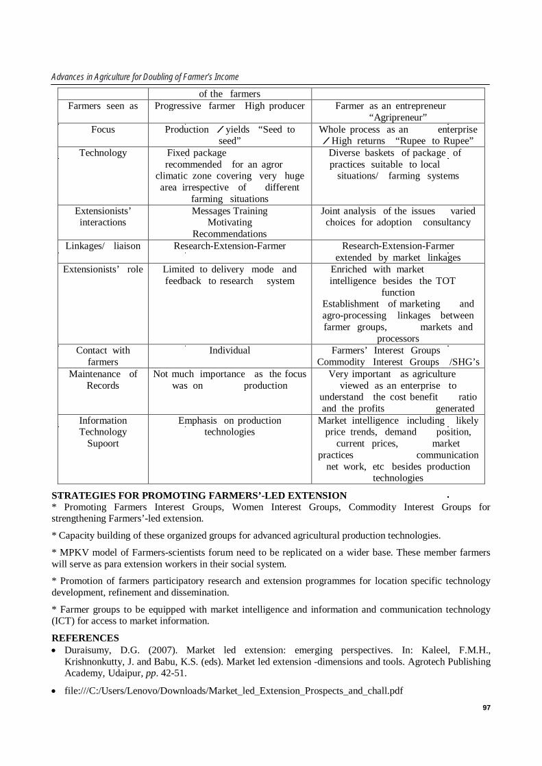
Advances in Agriculture for Doubling of Farmer’s Income
97
of the farmers Farmers seen as Progressive farmer High producer Farmer as an entrepreneur
“Agripreneur” Focus Production / yields “Seed to
seed” Whole process as an enterprise / High returns “Rupee to Rupee”
Technology Fixed package recommended for an agror
climatic zone covering very huge area irrespective of different
farming situations
Diverse baskets of package of practices suitable to local
situations/ farming systems
Extensionists’ interactions
Messages Training Motivating
Recommendations
Joint analysis of the issues varied choices for adoption consultancy
Linkages/ liaison Research-Extension-Farmer Research-Extension-Farmer extended by market linkages
Extensionists’ role Limited to delivery mode and feedback to research system
Enriched with market intelligence besides the TOT
function Establishment of marketing and agro-processing linkages between farmer groups, markets and
processors Contact with
farmers Individual Farmers’ Interest Groups
Commodity Interest Groups /SHG’s Maintenance of
Records Not much importance as the focus
was on production Very important as agriculture
viewed as an enterprise to understand the cost benefit ratio and the profits generated
Information Technology
Supoort
Emphasis on production technologies
Market intelligence including likely price trends, demand position,
current prices, market practices communication
net work, etc besides production technologies
STRATEGIES FOR PROMOTING FARMERS’-LED EXTENSION * Promoting Farmers Interest Groups, Women Interest Groups, Commodity Interest Groups for strengthening Farmers’-led extension.
* Capacity building of these organized groups for advanced agricultural production technologies.
* MPKV model of Farmers-scientists forum need to be replicated on a wider base. These member farmers will serve as para extension workers in their social system.
* Promotion of farmers participatory research and extension programmes for location specific technology development, refinement and dissemination.
* Farmer groups to be equipped with market intelligence and information and communication technology (ICT) for access to market information.
REFERENCES Duraisumy, D.G. (2007). Market led extension: emerging perspectives. In: Kaleel, F.M.H.,
Krishnonkutty, J. and Babu, K.S. (eds). Market led extension -dimensions and tools. Agrotech Publishing Academy, Udaipur, pp. 42-51.
file:///C:/Users/Lenovo/Downloads/Market_led_Extension_Prospects_and_chall.pdf

Advances in Agriculture for Doubling of Farmer’s Income
98
https://www.manage.gov.in/studymaterial/MLE-E.pdf
Kokate, K.D., Kharde, P.B., Patil, S.S. and Deshmukh, B.A. (2009) Farmers’- led extension: experiences and road ahead. Indian Res. J. Ext. Edu. 9, 18-21.
Moni, M. (2004). Ushering market-led agriculture extension. Available at http://www.i4donline.net

Advances in Agriculture for Doubling of Farmer’s Income
99
ECONOMIC ANALYSIS OF INCOME AND EMPLOYMENT GENERATION ON INTEGRATED FARMING SYSTEMS IN VINDHYA REGION OF M.P.
Virendra Kumar Vishwakarma1*, Prem Ratan Pandey2 and J.K. Gupta2 1Department of Agriculture Science, AKS University, Satna, MP 2Department of Transfer of Technology, Faculty of Agriculture, MGCGV, Chitrakoot, Satna
ABSTRACT Study had discussed about the economic point of view and their contribution in respect to generation of income and employment to the marginal and small farmers adopting Integrated Farming Systems. Three districts Bhopal, Vidisha and Sehore were selected randomly in entire seven district of Vindhyan Plateau. Phanda, Vidisha and Sehore were selected from one block to each selected district on the basis of adoption of Integrated Farming System prevailed in the area. Fifteen villages were taken in to consideration to entire selected blocks of study area. However, Five villages were selected among each selected blocks in list of main agricultural villages where Integrated Farming System was prevailing was prepared with the help of Department of Agriculture. One hundred eighty farmers were considered for present study. However, sixty farmers were selected from entire population of farmer in each selected blocks of study area. All selected farmers (60) were categorized under small, medium and large (20 small + 20 medium + 20 large), respectively have considered for present study. Primary data was collected from sample farmers and the required secondary data was collected from Department of Agriculture and other statistical sources. Data were collected by the researcher himself through survey method during the agriculture year 2016-17. Data depicted that the highest relative change in income and employment generation was found in farming system (3rd – Crops + Dairy) over crop husbandry alone. Data depicted that as regards relative change in income of farming system III was found to increase by (244.47%) and the employment days increased was 144.63% during a year over to base farming system i.e. crop husbandry alone Ist. (2nd – Crops + Vegetables) over crop husbandry alone Data depicted that as regards relative change in income of farming system II was found to increase by (169.61%) and the employment days increased was (118.18%) during a year over to base farming system i.e. crop husbandry alone. In the last, the relative change in income and employment generation was found in farming system (4th – Crops + Poultry) over crop husbandry alone. Data depicted that as regards relative change in income of farming system IV was found to increase by (152.52%) and the employment days increased was (120.66%) during a year over to base farming system i.e. crop husbandry alone. 3 most important farming systems were also prevailing at farm level. The data of relative change in income and employment generation from farming system IInd (Crops + Vegetables), IIIrd (Crops + Dairy) and IVth (Crops + Poultry) over to crop husbandry in study area found to increase in positive way. Accordingly, overall the income generation in these farming system were increased by (188.87%) over base farming system i.e. crop husbandry alone Ist. On the other hand, in respect to overall relative change in employment generation of these farming system were increased by (128.10%) over base farming system i.e. crop husbandry alone Ist. It can be concluded that the Integrated Farming System provided additional (188.87%) farm income and additional (128.10%) family labour to the farmers over crop husbandry alone. It is also suggested that village farmer’s cooperative societies should be formed in study area as it solves village level problems like marketing of different products, equipments problem through cooperative equipments, sharing of knowledge related to agriculture in proper way.
Keyword: Integrated Farming System, Crop husbandry, Employment, Income and Relative change.
INTRODUCTION Agriculture is not only the main source of livelihood but also a tradition and the most common way of life. It has been enjoying since times immemorial a place of pride in our economic and social life. Indian agriculture has responsibility of providing national as well as household food and nutritional security to its spilling over millions.

Advances in Agriculture for Doubling of Farmer’s Income
100
Agriculture plays a pivotal role in the Indian economy. Agriculture contributes about 18.00 per cent to the Gross Domestic Product (GDP) of India. About 60.0 per cent of the country’s population takes out their livelihood from this sector of the economy. The importance of agriculture in India prevails admits the fast growing secondary and tertiary sectors. It has estimated that more than 65.0 % of the total population of the country still lives in rural areas and 52 % of population depends on agriculture and related enterprises. Improved the income of the poor, cannot neglect the agricultural sector.
Integrated farming (also known as mixed farming) is a farming framework with synchronous exercises including yield and creature. An integrated effort to address the emerging issues in fact, our experience has clearly evinced that the income from cropping alone is hardly - sufficient to sustain the small and marginal farmer's needs.
With enhanced consumerism in rural areas, farmer's requirements for cash have also increased to improve their standard of living that is especially true in case of small and marginal farmers. Therefore, farmer's income and food security would have to be increase and supplemented by adoption of efficient allied enterprises like dairy, poultry, horticulture etc.
Integrated farming systems have much suitability like as deteriorating resource base, climate change, narrowed biodiversity, multiplicity of integrated farming systems, low rate of farm resource recycling and technology adoption gaps.
Integrated farming systems have many benefits like as productivity, profitability, sustainability, balanced food, environmental safety, income round the year, adoption of new technologies, saving energy, meeting fodder crisis, solving fuel and timber crisis, agro–industries and increasing input efficiency
Agriculture has a large potential to contribute to the national income while at the same time provide direct employment and income to the numerically larger and vulnerable sections of the society and to increase the exports to earn the much needed foreign exchange. Agriculture continues to hold the key to the progress of the country. Agriculture has also importance due to that it produces raw material for the industries.
Agriculture in Madhya Pradesh has characterized among other things, by the problem of wide year-to-year fluctuation in production and hence, the farm income varies. To compete with these sectors, the income from the agriculture must be increased which can be possible by rational use of resources and by raising production on the farms through the adoption of new technology.
The average cropping intensity of the zone was 143.10 per cent, which was higher than the Madhya Pradesh (135.40%). Amongst all the districts cropping intensity was maximum in Sehore district (176.20%) followed by Raisen (163.30%), Guna (143.40%), Bhopal (142.50%), Sagar (129.37%), Damoh (128.80%) and Vidisha (120.40%) districts.
Vindhaya region has some characteristics among other things, by the problem of low-income, poverty and low productivity unemployment. Therefore, more opportunity has available among Integrated farming systems to increase the income and employment.
Specific objectives - Study has covered the following objectives 1. To study the existing system of farming and their profitability
2. To study the relative change in income and employment generation over integrated enterprises
3. To study the Constraints faced by farmers in adoption of Integrated Farming System
METHODOLOGY Methodology of research is the blue print of research architect. This part of the research explains the approach, principles and procedures to be followed in conducting the study in the field. The research methodology and design are the main feet for waking, thus, making the research move ahead. This is involves various steps applied to the study of the problem. The material and methods are described in the following sub heads:

Advances in Agriculture for Doubling of Farmer’s Income
101
Selection of area and sampling procedure The present study confined to Vindhyan Plateau agro-climatic region of Madhya Pradesh. Seven districts come under Vindhyan Plateau i.e. Bhopal, Sagar, Damoh, Vidisha, Raisen, Sehore and Guna.
In present examination, among the Vindhyan Plateau area, locals, squares, towns and respondents as test of the investigation has been chosen through multi-arrange cum straightforward irregular or purposive inspecting system technique.
Selection of sample units Three districts of Vindhyan Plateau have been selected randomly out of seven districts in Vindhyan Plateau, three districts Bhopal, Vidisha and Sehore has been considered in present study.
One block has been selected from each selected district based on adoption of Integrated Farming System prevailed in the area. However, three blocks Bhopal, Vidisha and Sehore have selected among entire selected districts of Vindhaya Platue.
List of main agricultural villages where Integrated Farming System are prevailing was prepared with the help of Department of Agriculture in each selected blocks However, finally fifteen villages have select among list of entire villages of each selected block, top 5 villages were selected from available village list of Department of Agriculture in study area.
Among the consolidated list of farmers from selected villages in entire selected block was categorized into different classes i.e. small (0.1 to 2.0 ha.), medium (2.01 to 4.00 ha.) and large (above 4.00). Among each group 20 farmers were selected randomly for detail investigation in each block. However, 60 farmers were selected from each selected blocks of the study area. Thus, 180 farmers (60 small + 60 medium + 60 large) were considered for present study.
The nature, source of data and reporting period Present study has used both primary and secondary data. Used data have collected from different sources. All the collected primary data has related to the agriculture year 2016-17. Primary data have collected from sample farmers and with using survey method. The primary data have recorded mainly regarding socio economic and agrarian characteristics, return realized from different cropping system and problems in adoption of integrated farming system.
The required secondary data have collected from department of agriculture and other statistical data have collected from published record of Statistical Department.
Method of data collection and research instrument The researcher himself collected data through a door-to-door visit to the selected respondents with using the structured interview schedule. Data have collected through conduct with direct interview with the selected farmers.
An interview schedule was used as the research instrument in order to collect relevant information from the respondents. The interview schedule was prepared considering the objectives of the study in mind. The questions and statements contained in the schedule were simple, direct and easily understandable by the farmers without giving rise to doubt and misunderstanding in their minds. The schedule contained both opened and closed form of questions adopting the technique for measuring selected characteristics. The questions in respect of various costs and return from different farming system were also raised to find out the economics of production and resource use efficiency. Before finalization the interview schedule a pre-test was run in the study area in actual field situations. The pre-test was helpful to locate faulty questions. Alterations and adjustment were for the schedule on the basis of experience of the pre-test. During modification of the schedule the researcher incorporated valuable suggestions from his research supervisor and research co-supervisor into it. Finally, the schedule was replicate to 180 respondents.
Processing of data The collected raw data have examined thoroughly to detect errors and omissions. Actually, the researcher made a careful scrutiny of the completed interview schedules to make sure that they have entered as complete as possible and well arranged to facilitate descriptive statistics and economic analysis. Minor

Advances in Agriculture for Doubling of Farmer’s Income
102
mistakes were detected by doing this, which was corrected promptly. After completion of processing of data, it has been tabulated as per the specific objectives.
The analytical economic and statistical tools used Keeping in view the objectives of the study and to draw logical conclusion descriptive statistics and economic analysis were used for analyzing and interpreting the data.
The simple descriptive analysis was used to calculate to find out frequency, average values and percentages of different characteristics of the farmers in the study.
Average value:
The average or mean value was obtained by following formula
AM = ∑Y / N
Where; AM = Average value or Mean value
∑Y = Sum of all observations or variables
N = Total number of variables
Percentage:
The percentage of the farmer responses was obtained by using
P = F / N * 100
These were obtained in order to have comparison among different respondents
Where; F = Frequency of a class
N = Total number of observations
Profitability aspects:
For estimation of profitability, the following income measures were used.
a) Net farm income (NFI) = Gross income – Cost C3 (total cost)
b) Family labour income (FLI) = Gross income – Cost B2
c) Farm business income (FBI) = Gross income –Cost A1
d) Benefit Cost Ratio (BCR)
Benefit cost ratio was calculated by using following formula.
BCR = Gross Income/Cost C 3
The decision is made
i. If BCR > 1, project is worth while and accept it
ii. In case of a lot of projects or policies accept that which one has the highest BCR
RESULTS AND DISCUSSION The detail result and discussions presented has been highlights according to objectives of the study.
Identify the existing system of farming During the investigation it was observed that crop husbandry mainly cereals, pulses and oilseed found the main components in existing croppng system of study area. Crop husbandry alone does not generate enough income to keep a farm family out of poverty and provide the better standard of living.
In this situation the few farmers of study area have been diverted the crop husbandry alone farming system towards higher generating income farming system for higher family income and food security. This has happened supplemented by adoption of efficient allied enterprise like horticulture (vegetable cultivation), dairy (milk production) and poultry farming. The existing farming system may be called mixed farming

Advances in Agriculture for Doubling of Farmer’s Income
103
system which is combine of crop husbandry, crops + vegetables, crops + dairy, crops + poultry etc. The detail description of existing farming system in study area has been present in table 1.
Table 1: Land holding - wise farming systems existing in the study area
S.No. Existing farming system Size of holding (Ha.) Small Medium Large Total
1. Crop husbandry alone 24 (40.00)
16 (26.66)
7 (11.67)
47 (26.11)
2. Crops + vegetable 17 (28.33)
19 (31.67)
30 (50.00)
66 (36.67)
3. Crops + dairy 13 (21.67)
18 (30.00)
16 (26.66)
47 (26.11)
4. Crops + poultry 6 (10.00)
7 (11.67)
7 (11.67)
20 (11.11)
5. Total 60 (100.00)
60 (100.00)
60 (100.00)
180 (100.00)
Note: The figures in parenthesis show their respective percentage
In study area, mostly respondents are growing crops in kharif and rabi seasons and accordingly cropping activities are found in a similar trend viz. kharif and rabi crop’s season respectively.
The overall existing situation regarding farming system at the selected farmers level depicts that crop-combination with other allied activities found to maximum (73.89%), while the crop alone cultivation was found to minimum (26.11%) during the survey year. The higher adoption of integrated farming system or mixed farming system might be due to that this system providing employment and income round the year and generated extra employment and income made them economically active.
The existing crop enterprise-mix in the study area was dominated by crops + vegetable cultivation (36.67%). The next most important cropping system in the study area was crops + dairy adopted by (26.11%) of selected farmers followed by crops + poultry was adopted by (11.11%) of selected farmers.
The few farmers adopted crops alone in cultivation practices at their farm. It was observed that small farmers (40.00%) of total, adopted crop cultivation farming system followed by (26.66%) medium farmers and (11.67%) large farmers adopted crop farming system. The crop alone farming system was found to adopt by higher number of small farmers which is decreasing with increasing size of holding.
The adoption of crops + vegetable cultivation farming system was more might be due to cultivation of vegetables has been more profitable in the urban vicinity as better prices are assured in such a region. It was observed that large farmers (50.00%) of total, adopted crop + vegetables cultivation farming system followed by (31.67 %) medium farmers and (28.33%) small farmers adopted crop+ vegetable farming system. This farming system was found to adopt by higher number of farmers with increasing size of holding.
In study area, mostly farmers are rearing milch animal for milk production. It is found that the higher number of medium farmers (30.00%) adopted crops + dairy farming system followed by (26.66%) large farmers and (26.67%) small farmers adopted crop + dairy farming system.
It was observed that large and medium farmers (11.67%) each of total, adopted crop + poultry farming system followed by (10.00%) small farmers adopted crop+ poultry farming system. This farming system has found to adopt by higher number of farmers with increasing size of holding.
Table 2: Annual average profitability in adopted integrated enterprises (Rs/ha) S.
No.
Particulars
Integrated Enterprises Ist -Crop
husbandry alone (Major crops production)
(Rs/ha)
2nd – Crops +
Vegetables (Rs/ha)
3rd – Crops + Dairy
(Rs/ha and /milch
animal/year)
4th – Crops + Poultry
(Rs/ha and 100 birds unit
per year)
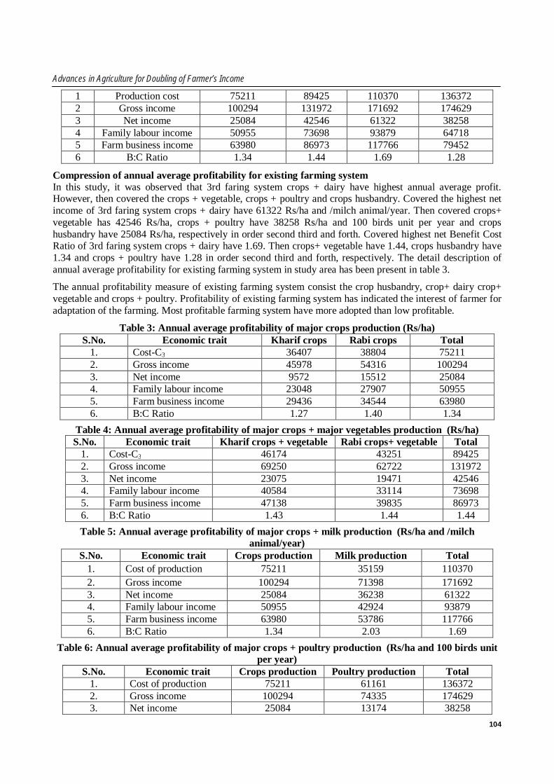
Advances in Agriculture for Doubling of Farmer’s Income
104
1 Production cost 75211 89425 110370 136372 2 Gross income 100294 131972 171692 174629 3 Net income 25084 42546 61322 38258 4 Family labour income 50955 73698 93879 64718 5 Farm business income 63980 86973 117766 79452 6 B:C Ratio 1.34 1.44 1.69 1.28
Compression of annual average profitability for existing farming system In this study, it was observed that 3rd faring system crops + dairy have highest annual average profit. However, then covered the crops + vegetable, crops + poultry and crops husbandry. Covered the highest net income of 3rd faring system crops + dairy have 61322 Rs/ha and /milch animal/year. Then covered crops+ vegetable has 42546 Rs/ha, crops + poultry have 38258 Rs/ha and 100 birds unit per year and crops husbandry have 25084 Rs/ha, respectively in order second third and forth. Covered highest net Benefit Cost Ratio of 3rd faring system crops + dairy have 1.69. Then crops+ vegetable have 1.44, crops husbandry have 1.34 and crops + poultry have 1.28 in order second third and forth, respectively. The detail description of annual average profitability for existing farming system in study area has been present in table 3.
The annual profitability measure of existing farming system consist the crop husbandry, crop+ dairy crop+ vegetable and crops + poultry. Profitability of existing farming system has indicated the interest of farmer for adaptation of the farming. Most profitable farming system have more adopted than low profitable.
Table 3: Annual average profitability of major crops production (Rs/ha) S.No. Economic trait Kharif crops Rabi crops Total
1. Cost-C3 36407 38804 75211 2. Gross income 45978 54316 100294 3. Net income 9572 15512 25084 4. Family labour income 23048 27907 50955 5. Farm business income 29436 34544 63980 6. B:C Ratio 1.27 1.40 1.34
Table 4: Annual average profitability of major crops + major vegetables production (Rs/ha) S.No. Economic trait Kharif crops + vegetable Rabi crops+ vegetable Total
1. Cost-C3 46174 43251 89425 2. Gross income 69250 62722 131972 3. Net income 23075 19471 42546 4. Family labour income 40584 33114 73698 5. Farm business income 47138 39835 86973 6. B:C Ratio 1.43 1.44 1.44 Table 5: Annual average profitability of major crops + milk production (Rs/ha and /milch
animal/year) S.No. Economic trait Crops production Milk production Total
1. Cost of production 75211 35159 110370 2. Gross income 100294 71398 171692 3. Net income 25084 36238 61322 4. Family labour income 50955 42924 93879 5. Farm business income 63980 53786 117766 6. B:C Ratio 1.34 2.03 1.69
Table 6: Annual average profitability of major crops + poultry production (Rs/ha and 100 birds unit per year)
S.No. Economic trait Crops production Poultry production Total 1. Cost of production 75211 61161 136372 2. Gross income 100294 74335 174629 3. Net income 25084 13174 38258

Advances in Agriculture for Doubling of Farmer’s Income
105
4. Family labour income 50955 13763 64718 5. Farm business income 63980 15472 79452 6. B:C Ratio 1.34 1.21 1.28
It has observed that, crop+ poultry have more cost but it have less benefit, then the crop + dairy have more cost but it has more benefit due to higher B:C Ratio, crop husbandry have low cost but it have less net income than other existing farming system crop + vegetable, crop+ poultry due lower B:C Ratio. Therefore, farmer have more prefer to crop + poultry then the crop+ dairy and other farming system.
Comparison of different system of farming in term of relative change in income and employment generation over crop husbandry: The farmers, agricultural planners and agricultural economists are interested to know the profitability of different farming systems in terms of income and employment generation. It is due to policymaking strategy for better development of farm and farm family and to increase the farm income that is the main source of farmers' livelihood.
The disparities in profitability in term of income and employment generation of different farming systems are mainly determine by relative change over crop husbandry alone a period of one year. For calculation of relative change in income and employment generation crop husbandry was treated as base (100.00%). The detail of relative change in different farming system in respect of income and employment generation over to crop husbandry (Farming system I) had presented in table 5.
Table 7: Relative changes in income and employment generation over crop husbandry (%) S.No. Farming system Income (Rs.) Employment (days)
1. 1st - Crop husbandry 25084 (100.00)
121 (100.00)
2. 2nd – Crops + Vegetables 42546 (169.61)
143 (118.18)
3. 3rd – Crops + Dairy 61322 (244.47)
175 (144.63)
4. 4th – Crops + Poultry 38258 (152.52)
146 (120.66)
Note: Figures in parenthesis denotes percentage over farming system
Data depicted that the highest relative change in income and employment generation has found in farming system (3rd – crops + dairy) over crop husbandry alone. Data depicted that as regards relative change in income of farming system III was found to increase by (244.47%) and the employment days increased was (144.63%) during a year over to base farming system i.e. crop husbandry alone Ist.
The next important relative change in income and employment generation was found in farming system (2nd – crops + vegetables) over crop husbandry alone. Data depicted that as regards relative change in income of farming system II was found to increase by (169.61%) and the employment days increased was (118.18%) during a year over to base farming system i.e. crop husbandry alone Ist.
In the last, the relative change in income and employment generation was found in farming system (4th – crops + poultry) over crop husbandry alone. Data depicted that as regards relative change in income of farming system IV was found to increase by (152.52%) and the employment days increased was (120.66%) during a year over to base farming system i.e. crop husbandry alone Ist.
Constraints faced by farmers in adoption of Integrated Farming System It was observe that during study survey that no selected farmers were adopted integrated farming system at farm level. Only few farmers were found to adopt vegetable cultivation, dairy production and poultry production along with crop production. The non adoption of Integrated Farming System at overall farm level in general could be due to various reasons. Some of the constraints faced by farmers had been presented in table 8. The constraints analysis was reported based on the opinion survey of the sample farmers.
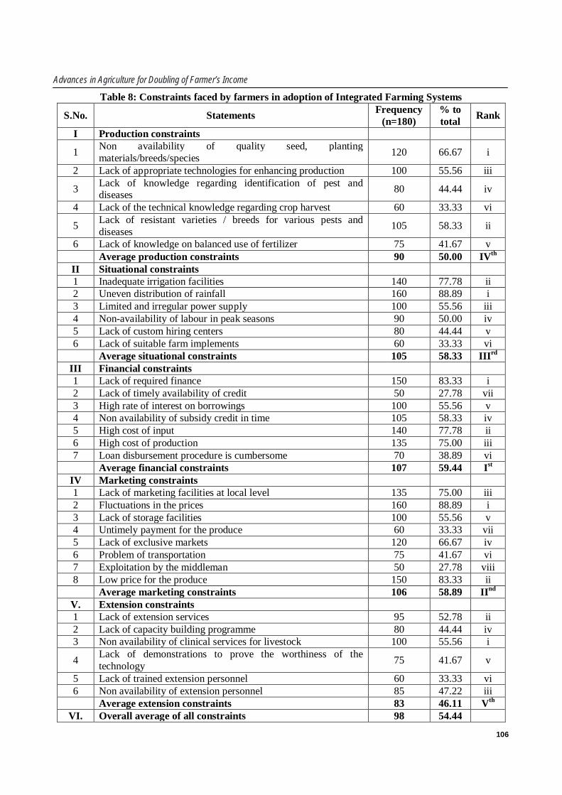
Advances in Agriculture for Doubling of Farmer’s Income
106
Table 8: Constraints faced by farmers in adoption of Integrated Farming Systems
S.No. Statements Frequency (n=180)
% to total Rank
I Production constraints
1 Non availability of quality seed, planting materials/breeds/species 120 66.67 i
2 Lack of appropriate technologies for enhancing production 100 55.56 iii
3 Lack of knowledge regarding identification of pest and diseases 80 44.44 iv
4 Lack of the technical knowledge regarding crop harvest 60 33.33 vi
5 Lack of resistant varieties / breeds for various pests and diseases 105 58.33 ii
6 Lack of knowledge on balanced use of fertilizer 75 41.67 v Average production constraints 90 50.00 IVth
II Situational constraints 1 Inadequate irrigation facilities 140 77.78 ii 2 Uneven distribution of rainfall 160 88.89 i 3 Limited and irregular power supply 100 55.56 iii 4 Non-availability of labour in peak seasons 90 50.00 iv 5 Lack of custom hiring centers 80 44.44 v 6 Lack of suitable farm implements 60 33.33 vi Average situational constraints 105 58.33 IIIrd
III Financial constraints 1 Lack of required finance 150 83.33 i 2 Lack of timely availability of credit 50 27.78 vii 3 High rate of interest on borrowings 100 55.56 v 4 Non availability of subsidy credit in time 105 58.33 iv 5 High cost of input 140 77.78 ii 6 High cost of production 135 75.00 iii 7 Loan disbursement procedure is cumbersome 70 38.89 vi Average financial constraints 107 59.44 Ist
IV Marketing constraints 1 Lack of marketing facilities at local level 135 75.00 iii 2 Fluctuations in the prices 160 88.89 i 3 Lack of storage facilities 100 55.56 v 4 Untimely payment for the produce 60 33.33 vii 5 Lack of exclusive markets 120 66.67 iv 6 Problem of transportation 75 41.67 vi 7 Exploitation by the middleman 50 27.78 viii 8 Low price for the produce 150 83.33 ii Average marketing constraints 106 58.89 IInd
V. Extension constraints 1 Lack of extension services 95 52.78 ii 2 Lack of capacity building programme 80 44.44 iv 3 Non availability of clinical services for livestock 100 55.56 i
4 Lack of demonstrations to prove the worthiness of the technology 75 41.67 v
5 Lack of trained extension personnel 60 33.33 vi 6 Non availability of extension personnel 85 47.22 iii Average extension constraints 83 46.11 Vth
VI. Overall average of all constraints 98 54.44

Advances in Agriculture for Doubling of Farmer’s Income
107
As per the farmers opinion overall (54.44%) farmers were faced problems in integrated farming system in different extent. The total constraints had been divided into 5 sub parts. The main constraint confronted by farmers were “financial constraints” rank Ist followed by “marketing constraints” (rank IInd), “situational constraints” (rank IIIrd), "production constraints" (rank IVth) and "extension constraints" (rank Vth), respectively.
Among the “financial constraints”, the important constrains was "lack of required finance" confronted by higher percentage of farmers (83.33%) followed by “high cost of input” reported by (77.78%), “high cost of production” reported by (75.00%), “non availability of subsidy credit in time” reported by (58.33%), “high rate of interest on borrowings” reported by (55.56%), “loan disbursement procedure is cumbersome” reported by (38.89%) and “lack of timely availability of credit” reported by (27.78%), respectively.
Among the “marketing constraints”, the important constrains was "fluctuations in the prices" confronted by higher percentage of farmers (88.89%) followed by “low price for the produce” reported by (83.33%), “lack of marketing facilities at local level” reported by (75.00%), “lack of exclusive markets” reported by (66.67%), “lack of storage facilities” reported by (55.56%), “problem of transportation” reported by (41.67%), “untimely payment for the produce” reported by (33.33%) and “exploitation by the middleman” reported by (27.78%), respectively.
Among the “situational constraints”, the important constrains was "uneven distribution of rainfall" confronted by higher percentage of farmers (88.89%) followed by “inadequate irrigation facilities” reported by (77.78%), “limited and irregular power supply” reported by (55.56%), “non-availability of labour in peak seasons” reported by (50.00%), “lack of custom hiring centers” reported by (44.44%), and “lack of suitable farm implements” reported by (33.33%), respectively.
Among the “production constraints”, the important constrains was "non availability of quality seed, planting materials/breeds/species" confronted by higher percentage of farmers (66.67%) followed by “lack of resistant varieties / breeds for various pests and diseases” reported by (58.33%), “lack of appropriate technologies for enhancing production” reported by (55.56%), “lack of knowledge regarding identification of pest and diseases” reported by (44.44%), “lack of knowledge on balanced use of fertilizer” reported by (41.67%), and “lack of the technical knowledge regarding crop harvest” reported by (33.33%), respectively.
In the last regarding “extension constraints”, the important constrains was "non availability of clinical services for livestock" confronted by higher percentage of farmers (55.56%) followed by “lack of extension services” reported by (52.78%), “non availability of extension personnel” reported by (47.22%), “lack of capacity building programme” reported by (44.44%), “lack of demonstrations to prove the worthiness of the technology” reported by (41.67%), and “lack of trained extension personnel” reported by (33.33%) respectively.
CONCLUSION Present study concluded that obtained the most existing integrated farming system have crop husbandry, horticulture (vegetable cultivation), dairy (milk production) and poultry farming. The existing farming system may be called mixed farming system that is combine of crop husbandry. Most of farmers have adopted the crops + vegetables, crops + dairy and crops + poultry. Dairy + crops and vegetable + crops integrated farming system in Vindhya region due to more profitable and easily generate the income.
3rd faring system crops + dairy have highest annual average profit than covered the crops + vegetable, crops + poultry and crops husbandry. Covered the highest net income of 3rd faring system crops + dairy Then covered crops+ vegetable, crops + poultry and and crops husbandry respectively in order first, second third and forth. Covered highest net Benefit cost Ratio of 3rd faring system crops + dairy, than crops+ vegetable, crops husbandry and crops + poultry in order to first, second third and forth, respectively.
The disparities in profitability in term of income and employment generation of different farming systems are mainly determine by relative change over crop husbandry alone a period of one year. Data depicted that the highest relative change in income and employment generation has found in farming system (3rd – crops + dairy) over crop husbandry alone. The next important relative change in income and employment generation was found in farming system (2nd – crops + vegetables) over crop husbandry alone. In the last,

Advances in Agriculture for Doubling of Farmer’s Income
108
the relative change in income and employment generation was found in farming system (4th – crops + poultry) over crop husbandry alone.
That constraint was analysis reported based on the opinion survey of the sample farmers. The main constraint confronted by farmers were “financial constraints” rank Ist followed by “marketing constraints” (rank IInd), “situational constraints” (rank IIIrd), "production constraints" (rank IVth) and "extension constraints" (rank Vth), respectively faced marketing constraints was fluctuations in the prices, low price for the produce, lack of marketing facilities at local level, lack of exclusive markets, lack of storage facilities, problem of transportation, untimely payment for the produce and exploitation by the middleman, respectively. The situational constraints was uneven distribution of rainfall, inadequate irrigation facilities, limited and irregular power supply, non-availability of labour in peak seasons, lack of custom hiring centers and lack of suitable farm implements, respectively.
The production constraint was non-availability of quality seed, planting materials, breeds, and species confronted by higher percentage of farmers. Followed other constraint as lack of resistant varieties / breeds for various pests and diseases, lack of appropriate technologies for enhancing production, lack of knowledge regarding identification of pest and diseases, lack of knowledge on balanced use of fertilizer, and lack of the technical knowledge regarding crop harvest, respectively.
Extension constraints was non availability of clinical services for livestock confronted by higher percentage of farmers lack of extension services, non availability of extension personnel, lack of capacity building programme, lack of demonstrations to prove the worthiness of the technology and lack of trained extension personnel reported, respectively.
REFERENCES Behera, U.K., Jha, K.P. and Mahapathra, I.C. (2001). Generation of income and employment-a success
story. Intensive Agric. 39, 9-13.
Channabasavanna, A.S., Biradar, D.P., Prabhudev, K.N. and Hegde, M. (2009). Development of profitable integrated farming system model for small and medium farmers of Tungabhadra project area of Karnataka. Karnataka J. Agric. Sci. 22, 25-27.
Das, T.K. (2015). Evaluation of farming system modules for improving profitability and livelihood of small and marginal farmers in Odisha. M.Sc. (Agri.) Thesis submitted to the Orissa University of Agriculture and Technology Bhubaneswar.
Deoghare, P.R., Sharma, B.M. and Goel, S.K. (1991). Impact of credit and technology on income and employment of small farms under different farming system in Karnal district (Haryana). Agricultural Situation in India 44, 65-70.
Deoghare, P.R., Sharma, B.M. and Goel, S.K. (1991). Impact of mixed farming system on income and employment on small farms in Karnal district of Haryana. Agric. Sit. India 45, 665-670.
Dwivedi, R.P., Tewari, R.K., Kareemulla, K., Chaturvedi, O.P. and Rai, P. (2007). Agrihorticultural system for household livelihood - a case study. Indian Research J. Extension Education 7, 22-26.
Gopinath, K.A., Dixit, S., Chary, R., Srinivasarao, G., Osman, M., Raju, B.M.K., Ramana, D.B.V., Venkatesh, G., Grover, M., Maheswari, M. and Venkateswarlu, B. (2013). Improving the rainfed farming systems of small and marginal farmers in Anantapur and Adilabad districts of Andhra Pradesh. Central Research Institute for Dryland Agriculture, Hyderabad, Andhra Pradesh, pp. 46.
Jayanthi, C., Vennila, C., Nalini, K. and Chandrasekaran, B. (2009). Sustainable integrated management of crop with allied enterprises- Ensuring livelihood security of small and marginal farmers. Sustainable Agriculture SF, 21-27
Harishkumar, H.V., Umesh, K.B., Kumar, M.S. and Venu, B.N. (2016). Livelihood security of farm households under different farming systems in Kolar District of Karnataka- an economic analysis. International Journal of Agriculture, Environment and Biotechnology 9, 313-322.

Advances in Agriculture for Doubling of Farmer’s Income
109
Kumar, M. (2014). Contribution of livestock production systems towards sustainable livelihood of the tribles of Jharkhand. M.Sc. Thesis, NDRI, Deemed University, Karnal
Murugan, G. and Kathiresan, R.M. (2005). Income and economic efficiency under low land integrated farming systems. Research on Crops 6, 234-236.

Advances in Agriculture for Doubling of Farmer’s Income
110
AN ECONOMIC ANALYSIS OF BRINJAL CULTIVATION IN CHHATTARPUR DISTRICT OF MADHYA PRADESH, UNDER TEJASWINI RURAL WOMEN EMPOWERMENT PROGRAM
Rajendra Singh Bareliya, J.K. Gupta* and Pradeep Kumar Patidar
Department of Transfer of Technology, MGCGV, Chitrakoot, Satna (MP), India
ABSTRACT It is observed from the data that an average total cost in cultivation of brinjal under beneficiary house hold (HH) (Rs.20911.12/acre) was found to be 13.45 per cent more than an average non-beneficiary HH (Rs. 18431.39/acre). The cost of production to produce a quintal of brinjal was also found to be 18.70 & 3.37 per cent less at total variable cost and total cost of cultivation of brinjal on an average beneficiary’s as compared to non-beneficiary’s HH farm, while net income received from production of brinjal was found to be 20.10 & 16.49 per cent more at total variable cost and total cost of cultivation respectively, resulted in increase of return per rupee investment by 29.48 & Rs. 1.83 per cent more at total variable cost and total cost of cultivation, on an average beneficiary’s as compared to an average non- beneficiary’s HHs farm, respectively.
Keywords: Production, Cost of Cultivation, Income and Profitability
INTRODUCTION Brinjal (Solanum melongena L.) more commonly known as eggplant is one of the most important vegetables grown throughout the country for its purple, green or white pendulous fruit. It is a member of the Solanaceae family and closely related to tomato and potato (Raza et al., 2018).
India is the second largest producer of vegetables in the world next to China. In India, brinjal is grown on 0.72 million hectares, equaling 10% of the total area under vegetable crops (NHB 2014), next only to China. Its yield, however, is low (18.6 t/ha), just half of that in China. One of the main reasons for low yield is inadequate and erratic supply of irrigation water (Narayanamoorthy, 2018). Brinjal is the fourth most important vegetable grown after potato, onion and tomato in India. It is planted in three seasons; first in Kharif (June-September), second in Rabi (November-February) and third in the month of March. This vegetable crop is primarily grown by small and marginal farmers and it is an important source of income for them. Brinjal production faces a number of problems which cause enormous yield losses. Fruit and shoot borer (FSB) is the most devastating insect-pest of brinjal, which causes 60-70% yield loss (Kumar et al., 2010). Vegetable production area of Madhya Pradesh is 2296.50'000 acre, out of which 52364 acres of area is being produced in brinjal, whereas the area of brinjal in Chhatarpur district is maximum because it produces very large quantities and large scale is done. The production of brinjal in Madhya Pradesh is being done in most Chhatarpur (4775.00 acres) and Sagar (3421.00 acres) districts.
OBJECTIVES 1. To work out the cost and return structure of brinjal cultivation
2. To identify the major constraints confronted by the farmers in brinjal cultivation.
RESEARCH METHODOLOGY A list of all the beneficiaries under Chattarpur (2014), has been provided by the office of the Madya Pradesh Vitta Vikas Nigam (MVVN), Bhopal. Further, 1 per cent of beneficiaries viz. 20 in Chhatarpur districts have been selected for the study. Thus, 20 beneficiaries along with the same number of non beneficiaries (20) were also selected from the same villages having same size of holding and socio economic status for the study, constituting total size of sample of 40 respondents. These beneficiaries were further classified as per the cultivation of vegetables grown by them in the area under study. Beneficiaries were found to grow several vegetables viz. brinjal, tomato, okra, potato, cucurbits, chili, cowpea, beans, cabbage, radish and leafy vegetables out of which on the basis of percentage of vegetables grown by the maximum numbers have been considered for the study (Table 1).

Advances in Agriculture for Doubling of Farmer’s Income
111
Table 1: Brinjal vegetables grown by beneficiaries and non-beneficiaries Vegetable Crops No. of respondents
Beneficiaries Non-Beneficiaries Total Brinjal 20 20 40
n= Numbers of Respondents
The primary data were collected from the selected respondents on various parameters viz. socio economic conditions, land use pattern, cropping pattern, cost of cultivation of brinjal vegetables and local practices, family consumption etc. control vs treated techniques was used to analyze the impact of brinjal production vis-a-vis local practices.
The suitable analytical tools were used to draw conclusions including compared means techniques. The study was conducted during the year 2018-19.
ANALYTICAL PROCEDURE Following concepts were used to draw conclusion.
1. Percentage Change over Non-Beneficiaries
Percentage Change = Yn (Beneficiaries)–Yo (Non- Beneficiaries)
x 100 Yo (Non- Beneficiaries)
2. Mean The average of the variables used for the study.
Where,
X = Mean of the variables
∑x = Sum of scores (observation) of variables
n = Total number of respondents
3. Interest of working Capital @10 per cent of variable inputs
4. Rental Value of owned land @1/6 of gross income
5. Interest on fixed capital @10 per cent of total capital assets (excluding land).
6. Managerial Cost @10 per cent of total cost to account for managerial input.
7. Cost of cultivation (per acre) = Operational Cost+Input Cost+Fixed Cost+Managerial Cost
8. Net income = Gross income-Total cost of cultivation
9. Cost of production (per q) = (Total cost of cultivation –value of by product)/ Yield
10. Cost Benefit Ratio = Gross Income /Total Cost
ESTIMATION OF COSTS AND RETURNS Results and Discussion Under the Tejaswini programme, for the production of vegetable in the first year, financial assistance of Rs. 3,000 for seed, fertilizer, plant protection measures and crop management is provided. Most of the beneficiaries are produced on large scale for the domestic consumption of brinjal vegetables and the remaining quantity is selling in the local market as well as outside.
Mean X = ∑x
n

Advances in Agriculture for Doubling of Farmer’s Income
112
Fig. 1. Districts wise area in percentage of brinjal crop of MP under the study
Brinjal crop was found to be a major vegetable grown by sample respondents both in kharif and rabi season by the respondents of the study area.
(A) Cost of Cultivation of Brinjal The cost of cultivation of brinjal for beneficiary and non beneficiary house holds (HHs) is presented in (Table 1). It is observed from the data that an average total cost in cultivation of brinjal under beneficiary HH (Rs.20911.12/acre) was found to be 13.45 per cent more than an average non-beneficiary HH (Rs. 18431.39/acre). An average beneficiary HH was found to used less expenditure on bullock labour (-16.70%), human labour (-16.10%), machine labour (-10.12%), family human labour (-7.85%), seed (-5.56%), irrigation (-7.09%), seed treatment material (-100.00%), while invested more on manures & fertilizer (95.39%) & insecticide (72.81) in cultivation of brinjal as compared to non beneficiary HH.
Fig. 2. Contribution of different cost in cost of cultivation of brinjal (beneficiaries)
Fig. 3. Contribution of different cost in cost of cultivation of brinjal (non-beneficiaries)

Advances in Agriculture for Doubling of Farmer’s Income
113
Table 2: Cost of cultivation of brinjal (Rs/Acre)
Particulars Beneficiaries Non-Beneficiaries % Change over Non-Beneficiaries
1.Operational Cost
A. Human labour-
Family 1680.00 (40.34)
1823.12 (38.05) -7.85
Hired 793.12 (19.04)
945.3 (19.73) -16.10
B. Machinery Power 93.66 (2.25)
104.21 (2.18) -10.12
C. Bullock labour 1598 (38.37)
1918.44 (40.04) -16.70
Total Operational Cost 4164.78 (100)
4791.07 (100) -13.07
2.Material Cost
A. Seed 850 (22.30)
900 (23.31) -5.56
B. Seed Treatment 0 (0.00)
20 (0.52) -100.00
C. Manure & Fertilizers 1723 (48.47)
1789 (46.34) 95.39
D. Insecticide 324 (9.11)
445 (11.53) 72.81
E. Irrigation 590 (16.60)
635 (16.45) -7.09
F. Depreciation 68.03 (1.79)
71.42 (1.85) -4.75
Total Material cost 3555.03 (100)
3860.42 (100) -7.91
Total Variable cost 7719.81 8651.49 -10.77 3. Fixed Cost
A. Rental Value of own land 11250.00 (156.53)
9737.50 (162.81) 15.53
B. Revenue /tax 12 (0.17)
12 (0.20) 0.00
C. Interest on Fixed capital 28.3 (0.39)
30.4 (0.51) -6.91
Total Fixed Cost 11290.30 (100)
9779.90 (100) 15.44
Managerial Cost 1901.011 1843.139 3.14 Total Cost of Cultivation 20911.12 18431.39 13.45
(Figures in parenthesis show the percentage to respective total)
The indirect cost (fixed cost) was found 15.44 per cent higher in case of an average beneficiary HH as compared to non-beneficiary HH. In total cost of cultivation of brinjal the share of total fixed was found to be 6 per cent higher on an average non beneficiary HH farm (48%) than an average beneficiary HH farm (54%), while share of total operation cost and total material cost in total cost of cultivation was found to be 4 and 2 per cent less on an average beneficiary HH farm than an average non beneficiary HH farm. The managerial cost was found to be identical in case of an average beneficiary (9%) and non- beneficiary HH farm (9%) in cultivation of brinjal. As in total cost of cultivation of brinjal the share of total operational cost, total material cost, total fixed cost and managerial cost were found to be 20 & 24, 17 & 19, 54 & 48 and 9 & 9 Per cent in case of beneficiaries and non- beneficiaries farms, respectively.

Advances in Agriculture for Doubling of Farmer’s Income
114
PROFITABILITY OF BRINJAL The cost of production to produce a quintal of brinjal was also found to be 18.70 & 3.37 per cent less at total variable cost and total cost of cultivation of brinjal on an average beneficiary’s as compared to non-beneficiary’s HH farm, while net income received from production of brinjal was found to be 20.10 and 16.49 per cent more at total variable cost and total cost of cultivation, respectively, resulted in increase of return per rupee investment by 29.48 and Rs. 1.83 per cent more at total variable cost and total cost of cultivation, on an average beneficiary’s as compared to an average non-beneficiary’s HHs farm respectively (Table 3).
Table 3: Profitability in cultivation of brinjal (Rs/Acre)
Particulars Beneficiaries
Non-Beneficiaries
% Change over Non-Beneficiaries
Yield (q/acre) 45 41 9.76 Rate/quintal (Rs.) 1500 1425 5.26
Main Product (Rs./acre) 67500 58425 15.53 Gross Return 67500 58425.00 15.53
Net Income Over Variable Cost Over Total Cost of
Cultivation
59780.19 49773.51 20.10
46588.88 39993.61 16.49
Cost of production
(Rs/q)
Over Variable Cost Over Total Cost of
Cultivation
171.55 211.01 -18.70
464.69 449.55 3.37
Return/Rs. investment
Over Variable Cost Over Total Cost of
Cultivation
8.74 6.75 29.48
3.23 3.17 1.83
(B) Constraints in Brinjal Cultivation A total postharvest loss of brinjal was 23.38%. Highest loss was estimated that 12.51% at the grower level. Among different intermediaries post harvest loss of brinjal was highest at retail level (5.96%) than Aratia level losses (2.35%) and trader level losses (2.65%) (Kaysar et al., 2016). Sixteen insecticides under different trade names were most commonly sprayed. Maximum brinjal growers were sprayed this insecticides more than 40 times during the period of whole cultivation. A diverse range of constraints impede brinjal production. These include pests and abiotic factors. The major groups of pests and abiotic factors impeding brinjal production, were insects (34%), fungi (23%), bacteria (13%), nutrient efficiency (12%), mites (8%), viruses (3%), nematodes (2%), and water moulds (2%). It is highly likely that frequencies of biotic and abiotic constraints were influenced by time, tomato variety and location (Willis et al., 2019)
CONCLUSION AND POLICY IMPLICATIONS Most of the vegetables available in the market are out of the reach of a common man due to their high prices, particularly in the recent period. The per capita availability of vegetables in the country is 190 gram per day as against the normative requirement of 280 gram per day. The vegetable deficit underscores the need for substantial increase in vegetable production and affordability to consumers.
REFERENCES Barker, N., Kumar, D. and Singh, N. (2017). An economic analysis of brinjal in Allahabad district of
Uttar Pradesh state. International J. Recent Scientific Research Research 8, 15925-15929.
Kaysar, M.I., Mia, M.S., Islam, M.S. and Kausar, A.K.M.G. (2016). Post harvest loss assessment of brinjal in some selected areas of Bangladesh. J. Business, Management and Social Research 2, 118-124.
Kumar, S., Prasanna, P.A.L. and Wankhade, S. (2011). Potential benefits of Bt brinjal in India-an economic assessment. Agricultural Economics Research Review 24, 83-90.
Kumar, U. and Agarwal, P.K. (2018). An economic analysis of brinjal cultivation in Birni block of Giridih district, Jharkahand. International J. Agriculture Sciences 10, 7147-7149.

Advances in Agriculture for Doubling of Farmer’s Income
115
Nandeshwar, N.S., Jagannath, Pritesh, T. and Shashikumar, M. (2013). Economics of production and marketing of vegetables in Akola district. Global J. Biology, Agriculture and Health Sciences 2, 78-82.
Narayanamoorthya, A., Bhattaraib, M. and Jothic, P. (2018). An assessment of the economic impact of drip irrigation in vegetable production in India. Agricultural Economics Research Review 31, 105-112.
Ochilo, W.N., Nyamasyo, G.N., Kilalo, D., Otieno, W., Otipa, M., Chege, F., Karanja, T., Lingeera, E.K. (2019). Characteristics and production constraints of smallholder tomato production in Kenya. Scientific African 2, 1-10.
Raza, M.S., Rahman, M.A., Rahaman, K.M.M., Juliana, F.M., Hossain, S., Rahman, A., Hossain, K., Alam, M.J. and Asaduzzaman, M. (2018). Present status of insecticides use for the cultivation of brinjal in Kushtia region, Bangladesh. International Journal of Engineering Science Invention 7, 44-51.

Advances in Agriculture for Doubling of Farmer’s Income
116
COMPARATIVE ECONOMICS OF FISH SELF-HELP GROUPS OF PRODUCTION AND MARKETING OF EXOTIC AND LOCAL BREEDS OF FISH IN KABIRDHAM
DISTRICT OF CHHATTISGARH
Virendra Kumar Vishwakarm1*, J.K. Gupta2 and K.N.S. Banafar3 1*Department of Agril. Economics, A.K.S. University Satna Madhya Pradesh 2Department of Transfer of Technolgy (Agril. Economics), MGCGV, Chitrakoot, Satna (MP) 3Department of Agril. Economics, Collage & Research Station, Janjgir- Chanpa (C.G.)
*[email protected] ABSTRACT Study has examined a comparative economics of Fish Self-Help Groups (FSHG) to production and marketing of exotic and local breeds of fish in Kabirdham districts of Chhattisgarh. The sampling was based on stratified randomly selected samples of FSHG in the study area. The selected samples of exotic breeds fish producer have 04 FSHG. However, the selected samples of local breeds fish producer have 12 fish self-help groups. The required primary data was collected from the selected respondent by the survey method during the year 2015-19. The study of compound growth rate of area, production and productivity of fish showed the positive and significant growth rate in both Chhattisgarh state and Kabirdham districts except area under fish in district Kabirdham. The fish productivity of exotic breeds of samples FSHG was 30.84 qt per ha. However, the fish productivity of local breeds of samples FSHG was 17.03 qt per ha, respectively. The per hectare cost of exotic breeds of samples FSHG was Rs. 54310.00 per ha. However, the per hectare cost of local breeds of fish of samples FSHG was Rs. 28198.40 per ha. The net return of exotic breeds of samples FSHG, was Rs. 254126.21 per ha. However, the net return of local breeds of samples FSHG is Rs. 95229.73 per ha, respectively. The cost benefit ratio of exotic breeds of samples FSHG was 4.68: 1. However, cost benefit ratio of local breeds of samples FSHG was 2.79: 1 The four marketing channels have been adopted in the study area and the most of FSHG have sold the fish in channel fifth and sold quantity of fish, by FSHG was 2338.00 qt. and 75.049 in the channel fifth. The net received price and incurred marketing cost of samples FSHG were Rs. 5000.00 & Rs. 298.7 per qt, Rs. 8398.74 & Rs. 1992.12 per qt and Rs. 7528.11 & Rs. 1883.95 per qt in the channel first, third, fourth and fifth, respectively in the channel first, second, third, fourth and fifth, respectively. The marketing efficiency and producer share in consumer rupees of samples FSHG were 9.23 % & 69.00 %, 2.22 % & 68.00 %, 2.23 % & 76.21 % in the channel third, fourth and fifth, respectively. It has been observed that the channel first has most efficient for FSHG. The major socio economics constraints found that, restriction on medicine, feed and manure, lease processed poaching of fish and consumption & fish disposal etc. in the fish production, which in a weak position the fish production of both groups of fish producers. Fish producers are faced various constraints i.e. water stress, lack of the improved production technology unavailability of market and poor marketing facilities and poor credit and fiancé availability, poor storage facility and social and villager class conflict.
Keywords: Cost, Return, Cost Benefit Ratio, Local and Exotic Breeds of fish, Marketing cost, Marketing Efficiency and Producer share in consumer rupee
INTRODUCTION Fish is one of the important items of food all over in the world. Due to steady growth of Indian population and increase problem of malnutrition, Considerable attentions have been given to enrich the biological value of the fish product in state of Tamil Nadu (Formerly Madras), Bengal, Punjab, Uttar Pradesh, Baroda, Maysore and Hyderabad. Fisheries sector occupies an important place in socioeconomic development of state. Three major carps of India are catla (catla catla) rohu lebeo (Labeo Rohita) and mrigal (Cirhinus mrigla). These carps contribute 90 % of the total Indian aquaculture production. 30700 species of fish have been found in Asia, and 2500 species have been found in India, in which 801 are fresh water species. However, fresh water carps are the most important species in India. In 1970, poly culture system was introduced in India. Later comes three exotic carps, Silver carp (Hypophthalchthys molitria), Grass carp

Advances in Agriculture for Doubling of Farmer’s Income
117
(Ctenopharyngodon idethes) and Common carp (Cyprinus carpio) that are considered to be important groups.
The traditional practice of fish culture in small pond in eastern India has known to have existed for hundred of years. Significant advance have made in the state of West- Bengal in the early nineteenth century with the controlled breeding of carp of bandhi (tank or impoundments) were reverine condition simulated. The fish culture received notable concentration in the state of Tamil Nadu (formerly madras), West-Bengal, Punjab, Uttar Pradesh, Baroda, Maysore and Hyderabad. Fish culture has established the fisheries department and support to fishes and fish farmers for the expansion of this sector.
The different fish marketing units have conducted the fish marketing in different areas of India. Total 33 fish marketing unit constituent by Indian govt. in 10th plan and followed as Andhrapradesh -2, Arunachal Pradesh-2, Haryana-2, Himanchal Pradesh-1, Jharkhand1, Karnataka-9, Madhya Pradesh-2, Maharastra-3, Mizoram-3, Odisha-1, Rajasthan - 1, Tamil Nadu-1, Tripura-1, Delhi (FISHCOPED)-2, Manipur 2 and Goa-1
The domestic fish market has not fully developed on modern lines there are gradual transformation from traditional to modern method of marketing with the advent of improved transport, processed and storage facilities at micro level. There are large numbers of small merchant. There are three or four types of functionaries at this level. Broker or commission agent, whole seller and retailer or village retailer and village merchant at last level finally fishes disposed to the consumer or export or processed etc.
As per the estimation of the central statistics organization (CSO) of the government of India, The value of G.D.P. from fishery sector of current price during 2011-12 is Rupee 65541 crores, with 4.47 percent of the total G.D.P. in agriculture and allied sector.
The national mean production level from still water ponds has gone up from 600 kilogram per hectare & per year in 1974 to over 2900 kilogram per hectare & per year at present and several farmers have even demonstrating, higher production level of 8-12 tonnes per hectare & per year (handbook of fisheries and aquaculture, ICAR publication, India).
Many self-help groups have also involved in fish production, transportation, input arrangements, harvesting, and marketing of the produce. These fish self-help groups play the important role in the fish production and marketing of fishes. Poor and marginal fishermen who have not survived the fisheries enterprises as individual than those are connected to each other as groups and doing work together and shared finance and physical activities as together and these groups are called Fish self help groups.
This research work done in fish production, marketing and constraints in the fish production and marketing in Kabirdham district of Chhattisgarh in year 2013-18 with the following objectives:
1. To analyze the growth rate of adding membership and constitution of self help groups Chhattisgarh
2. To work out the cost, return and profitability from fish production in the present study
3. To examine the marketing cost and price spread under different fish marketing channels.
4. To assess the constraints in production and marketing of fishes and to suggest suitable measures to overcome the problems
METHEDOLOGY Multistage stratified random sampling procedure has been adopted in this study. There were two stratum divide to all random selected respondent. The participants were selected randomly from each stratum until the decided sample size i.e. sixteen respondents were selected in the entire blocks of Kabirdham district by random sample method. However, randomly selected several special sample i.e. twelve fish producers, twelve fish producer trader, twelve village trader, eight retailers, four wholesalers in the marketing analysis. However, randomly select the several special sample i.e. four fish co-operative societies include some consumers in constraint analysis of the study area. The primary data was collected through the personal interview from selected sample of fish cooperative societies. However, secondary data were collected through personal contact from journal, internet, and information of fish to directorate of fishery,

Advances in Agriculture for Doubling of Farmer’s Income
118
Chhattisgarh, and deputy directorate of fishery, Kabirdham district. In addition, primary data has concerned about marketing and constraints i.e. local fish producer trader, village trader, wholesalers, retailers, and others market functionaries for analysis of fish marketing. We put the questions to ask the sample fish producers from structure questionnaire & schedule at time of interview for gathering primary information. The filled questionnaire & schedule were checked and scrutinized immediately after the interview and the collect information. The statistical tools were used in analysis of collected data. The data related to each management and marketing regime were assembled and reduced to comparable form by using different statistical tools. Then information has processed and tabulated for use the research analysis.
Marketing channels The different marketing channels have been involved in fish marketing and which has fish passed through different route from producer to consumer in the study area. No sufficient fish markets were available due to low level of fish production, thus most of tinny fish producer have to sale their own product direct to consumer, but some medium and large fish producer have adopted the following indirect fish marketing channel in the study area.
Producer- Consumer
Producer- Producer trader- Consumer
Producer- Village trader / Village retailer- Consumer
Producer- Fish co-operative societies or Fish self-help groups
Producer - Wholesaler- Retailer Consumer
Compound growth rate or Exponential rate Y= A. B t
Log y= log A + t log B
Compound Growth rate in percent =
(Anti log of B-1) × 100
Where, Y= Area / Production / Productivity compound growth rate,
A= Constant, B= Regression coefficient, t= time in year
Coefficient of variance = (Standard deviation) / Mean × 100
Absolute change = Value of current year – Value of base year
Relative change = (Value of current year – Value of base year) / (Value of base year) × 100
Variable cost = Labour wise cost (Pond preparation+ Feed application+ Initial liming and fertilizer application+ Seed or fingerling application+ Treatment+ Netting+ Storage cost+ Water refilling+ Repairing of bunds and embankment+ Fish rearing) + Input wise cost (Seed or fingerling+ Feed+ Lime and fertilizer+ Medicine and chemical) + Interest of working capital+ Miscellaneous material
Fixed cost = (Rent amount+ Rental value of pond+ Depreciation+ Interest of fixed capital)
Total Cost = Variable Cost +Fixed Cost
Gross Return =Total fish production × sale price of fish
Net Return = Gross return – Gross Expenses or total fish farming cost
Benefit Cost Ratio = B / C
Breakeven levels of fish produce analysis:
i. Price per quintal of fish=
(Total cost (Fixed cost + Variable cost) ) / (Total production)

Advances in Agriculture for Doubling of Farmer’s Income
119
ii. Production of fish=
(Total cost (Fixed cost + Variable cost) / (Price per unit)
Marketing information:
Marketing cost:
MC= Cf + Cm ith 1+Cm ith 2+………+ Cm ith
Where, MC = Total marketing cost of fish marketing. Cf = Cost paid by fishermen, Cm ith = Cost incurred by ith middlemen
Gross margin:
M= S ith + P ith
Where, M= Gross margin, S ith = Sale value of produce for ith middlemen, P ith = Purchase value for ith middlemen.
Net Margin:
Nm ith = Pr ith – (Pp ith +Cm ith)
Where, Nm ith = Net margin of ith type of market Middlemen, Pr ith = total value of received per unit (sale price), Pp ith = per unit purchase price of produce by the ith middlemen, Cm ith = cost incurred by the ith middlemen
Farmer Price:
Pf = PA- Q
Where, Pf= Net price received by the farmer, PA= Whole sale price, Q= Marketing cost incurred by the fishermen
Estimation of fish farmer’s share or producer share in consumer rupees:
Ps = Pf / Pr × 100
Where, Fishermen or producer share in consumer rupee, Pf= Net price received by the farmer, Pr= Price paid by the consumer.
Estimation of the marketing pattern:
C= Cf+ Cm ith 1+ Cm ith 2+… Cm ith
Where, C= Total marketing cost of producer, Cf = Cost paid by the farmers, Cm ith = Cost incurred by ith of intermediary.
Estimation of marketing efficiency:
E = O / I × 100
Where, ‘E’ =index of marketing efficiency, ‘O’ = Output (added value / market margin), ‘I’ = Input (marketing cost)
Constraints Analysis: Garrett’s ranking technique
Percentage position = (100 (R ij –0.05))/(N j)
Where, R ij = Rank give for the ith item by jth individual, N j = Number of item rank by the jth individual.
(Asking the question to sample fish producer and others respondents rank then ranked specific problems, which have faced by fish producer then according to their own perception in this method. The assigned rank is converting into percentage position, which has subsequently transferred into Garrett score using Garrett’s

Advances in Agriculture for Doubling of Farmer’s Income
120
table. For each constraint, scores of individual respondents are add together and then divided by total number of respondents. Thus, mean score for each constraint has ranked by arranging them in descending order)
RESULTS AND DISCUSSION Following results have been obtained with analysis of various objectives of research.
Table 1: Indices of constitution and added membership in Fish self-help groups I - Chhattisgarh state
II – Kabirdham District
Source: Deputy Directorate of Fisheries, Kabirdham district
INDICES OF CONSTITUTION AND ADDED MEMBERSHIP IN FISH SOCIETIES AND SELF- HELP GROUPS Proportionate change of constitution and added membership of fish self-help groups in Kabirdham district was analysed during the year 2010-11 to 2014-15 (period five years) (table 1 (II)]. Constitution of fish self-help groups in Kabirdham district was found to be the highest proportionate change with magnitude of 156.66 and to be lowest proportionate change with magnitude 29.98 per cent. Added membership of fish self-help groups in Kabirdham district was found to be highest proportionate change with magnitude of 149.16 and to be lowest proportionate change with magnitude 37.24 per cent. However, proportionate change of constitution and added membership of fish self-help groups in Chhattisgarh was analysed during the year 2004- 05 to 2012-13 (period nine years) [Table 1 (I)]. Constitution of fish self-help groups in Chhattisgarh was found to be highest proportionate change with magnitude of 130.42 and to be lowest proportionate change with magnitude of 84.83 per cent. Added membership of fish self-help groups in Chhattisgarh was found to be highest proportionate change with magnitude of 130.95 and to be lowest proportionate change with magnitude of 80.73 per cent.
Table 2: Variability in Constitution and added membership of fish self-help groups
* C.V. =Coefficient of co-variance
S. No.
Year
Fish self- help groups Proportionate change in constitution Proportionate change in membership
1 2004-05 100.00 100.00 2 2005-06 85.61 95.18 3 2006-07 87.35 94.90 4 2007-08 110.02 86.77 5 2008-09 84.83 80.73 6 2009-10 103.24 137.05 7 2010-11 115.35 107.28 8 2011-12 85.12 98.12 9 2012-13 130.42 130.95
S. No.
Year
Fish self- help groups Proportionate change in
constitution Proportionate change in
membership 1 2010-11 100.00 100.00 2 2011-12 156.66 149.16 3 2012-13 29.98 37.24 4 2013-14 150.00 124.00 5 2014-15 104.76 126.61
S. No. Particulars District Kabirdham (C.V.)* Chhattisgarh state (C.V.)* 1 Constitution 43.474 12.069 2 Added membership 33.047 15.838

Advances in Agriculture for Doubling of Farmer’s Income
121
VARIABILITY IN CONSTITUTION AND ADDED MEMBERSHIP OF FISH SOCIETIES AND SELF-HELP GROUPS Variability estimated by coefficient of co-variance for constitution and added membership of fish self help groups in Kabirdham district and Chhattisgarh has analysed (Table 2). During the year 2010-11 to 2014-15 (period five years) variability estimated by coefficient of variance for constitution of fish self help groups in Kabirdham district was found to be magnitude of 43.474 per cent. During the year, 2010-11 to 2014-15 (period five years) variability estimated by coefficient of variance for constitution of fish self help groups in Chhattisgarh was found to be magnitude of 12.069 per cent. However, it was observed that, during the year 2004-05 to 2012-13 (period nine years) variability estimated by coefficient of variance for added membership of fish self-help groups in Kabirdham districts was found to be magnitude of 33.047 per cent. During the year, 2004-05 to 2012-13 (period nine years) variability estimated by coefficient of variance for added membership of fish self-help groups in Chhattisgarh was found to be magnitude of 15.853 per cent.
Table 3: Compound Growth rate of adding membership and formation of Fish self help groups S. No. Particulars Chhattisgarh Kabirdham
1 Society formation -1.3%* -13.3%*
2 Adding membership 1.3%* -9.9%*
*significant (at the 5 % significant level)
COMPOUND GROWTH RATE OF ADDING MEMBERSHIP AND FORMATION OF FISH SELF HELP GROUPS The compound growth rate of adding membership of fish self-help groups of the Chhattisgarh was positive and significant but compound growth rate of constitution of fish self-help groups was negative and significant of the Chhattisgarh. The compound growth rate of constitution and adding membership of fish self help groups of Kabirdham district was negative & significant during the years 2013-15 (Table 3).
FISH PRODUCTION AND COST MEASUREMENT FOR SAMPLE FISH PRODUCER IN STUDY AREA The fish production cost was computed to fish producer independently work out sample of fish self-help groups. Fish production cost of exotic breeds sample of fish self-help groups have Rs. 54871.00 per hectare. However, fish production cost of local breeds sample of fish self-help groups have Rs. 28875.45 per hectare.
Entire types of fish producers have used the most of labour in pond preparation, feeding, netting and seed application practices in together local and exotic breed of fish production. Under variable cost, labour wise involved cost in pond preparation of exotic breeds sample of fish self-help groups have Rs. 909.46 per hectare with 1.65 per cent. However, feeding expenses of exotic breeds’ sample of fish self-help groups has Rs. 337.44 per hectare with 0.61 per cent (Table 4). However, netting expenses of exotic breeds sample of fish self-help group has Rs. 1234.56 per hectare with 2.27 per cent. However, seed application expenses of exotic breeds sample of fish self-help group has Rs. 415.63 per hectare with 0.74 per cent. Labour wise cost in pond preparation of local breeds sample of fish self-help groups Rs. 753.12 per hectare with 2.60 per cent. However, feeding cost of local breeds sample fish self-help groups has Rs. 244.20 per hectare with 0.83 percent. However, netting cost of local breeds’ sample of fish self-help groups has Rs. 880.36 per hectare with 3.04 per cent. However, seed or fingerling application cost of local breeds among sample of fish self-help groups has Rs. 316.02 per hectare with 1.09 per cent. Under the variable cost in material wise seeds or fingerling cost of exotic breeds of sample fish self-help group have Rs. 37314.87 per hectare with 67.54 per cent. However, feeds cost of exotic breeds fish self-help groups has Rs. 823.04 per hectare with 1.49 per cent. However, interest of working capital of exotic breeds’ sample of fish self-help groups has Rs. 4661.68 per hectare with 8.42 per cent. Material wise cost in seedling or fingerling of local breeds sample of fish self-help groups have Rs. 14216.08 per hectare with 49.04 per cent. However, Feed cost of local breed sample of FSHG has Rs. 614.28 per hectare with 2.21 per cent. Interest of working capital of local breed sample of fish self-help group has Rs. 2376.35 per hectare with 8.20 per cent. Under the fixed cost of pond rent of exotic breeds sample of FSHG have Rs. 2487.65 per hectare with 4.50 per cent. However, rental value of pond cost of exotic breeds sample of FSHG have and Rs. 1500 per hectare with 2.71 per cent. However, depreciation of pond of exotic breeds’ sample of FSHG has Rs. 248.76 per hectare with 0.45 per cent. However, interest of pond of exotic breeds’ sample of FSHG have Rs.171.59 per hectare with 0.31 per cent. However, pond

Advances in Agriculture for Doubling of Farmer’s Income
122
rent cost of local breed sample of FSHG have Rs. 1424.17 per hectare together with 4.91 per cent. However, rental value of pond of local breed of sample of FSHG have Rs. 1000 per hectare with 3.45 per cent. However, depreciation of pond for local breed of sample has Rs. 142.41 per hectare with 0.48 per cent. However, Interest of fixed capital in pond of local breed sample of FSHG have and Rs. 168.97 per hectare with 0.57 per cent.
Table 4: Fish production cost measure of Fish self- helps Groups in study area S. No. Particulars Fish self Helps Groups
Local (Rs / ha) Exotic (Rs / ha) I Variable/Working Cost A Labour wise cost 1 Pond preparation 753.12 (2.60) 909.46 (1.65) 2 Feed application 244.2 (0.83) 337.44 (0.61) 3 Initial liming & application
fertilization 396.05 (1.37) 465.02 (0.83)
4 Seed / Fingerling application 316.02 (1.09) 415.63 (0.74) 5 Treatment Expenses 68.74 (0.24) 82.30 (0.15) 6 Watching Expenses 4432.58 (15.28) 2962.96 (5.35) 7 Netting 880.36 (3.04) 1234.56 (2.22) 8 Storage Expenses 123.12 (0.41) 123.45 (0.22) 9 Water Refilling 864.45 (2.97) 576.13 (1.03) 10 Repairing of bond & embankment 0 0 11 Fish Rearing 81.05 (0.28) 130.04 (0.23)
Sub total 8159.69 7236.99 B Input / Material wise cost 1 Feeds 641.28 (2.21) 823.04 (1.49) 3 Lime and manure/ fertilizers 315.00 (1.09) 408.43 (0.74) 4 Treatment / Medicine 431.45 (1.49) 833.53 (1.51) 5 Seed / Fingerling 14216.08 (49.04) 37314.87 (67.54) 6 Miscellaneous 0 0 Sub total 15603.81 39379.87
C Interest of working capitals 2376.35 (8.20) 4661.68 (8.42) D Total working/ variable cost 26139.9 (90.17) 50463.37 (90.82) II Fixed / Overhead cost A Rent of ponds 1424.17 (4.91) 2487.65 (4.50) C Depreciation 142.41 (0.48) 248.76 (0.45) D Rental value of pond 1000.00 (3.45) 1500.00 (2.71) E Interest of fixed capital 168.97 (0.57) 171.59 (0.31) F Total fixed cost 2735.55 (9.44) 4408.00 (8.70)
III Total cost 28875.45 (100.00) 54871.00 (100.00)
PROFITABILITY MEASURE IN FISH PRODUCTION OF SAMPLE FISH PRODUCERS IN STUDY Gross return, net return, cost benefit ratio, fish production, selling price, total cost, cost of production, and Break-even point in fish production of sample fish producers for local and exotic breeds were calculated independently. Fish production of exotic breeds of FSHG have 30.84 quintal per hectare. However, fish production of local breeds FSHG have 17.03 quintal per hectare. Price of exotic breeds of FSHG have Rs. 10000.00 per quintal. However, fish production of local breeds of FSHG has Rs. 7246.56 per quintal. Fish production cost of exotic breeds of FSHG have Rs. 54871.00 per hectare. However, fish production cost of local breeds of FSHG have Rs. 28875.45 per hectare. Gross return of exotic breeds of FSHG Rs. 308400.00 per hectare. However, gross return of local breeds’ FSHG have Rs. 123408.91 per hectare. Net return of

Advances in Agriculture for Doubling of Farmer’s Income
123
exotic breeds’ FSHG has Rs. 253529.00 per hectare. However, net return of local breeds’ FSHG has Rs. 94533.46 per hectare. Net return for local breeds have low than exotic breeds due to price of exotics breeds is high and its productivity is also high. Cost benefit ratio of exotic breeds of FSHG have 4.61:1. However, cost benefit ratio for local breeds of FSHG has 3.26:1. Cost of fish production of exotics breeds’ FSHG has Rs. 1779.22 per hectare. However, cost of fish production of local breeds Rupee 1695.56 per hectare. Break-even points of exotic breeds’ FSHG have 5.95, 9.79 and 5.47. However, break-even points of local breeds’ FSHG have 5.47, respectively (Table 5).
Table 5: Profitability measure in fish production of Fish self Helps Groups in study area
S. No. Particulars Local Exotic 1 Production in qt per ha 17.03 30.84 2 Price in Rs Per qt. 7246.56 10000.00 3 Fish production cost in Rs per ha 28875.45 54871.00 4 Gross Return in Rs per ha 123408.91 308400.00 5 Net Return in Rs per ha 94533.46 253529.00 6 Cost benefit ratio in percent 3.26 :1 4.61 :1 7 Break-even level of output of fish a i. Price 1695.56 1779.22 b ii. Production 3.98 5.47
COST DISTRIBUTION IN FISH PRODUCTION OF SAMPLE FISH PRODUCER IN STUDY AREA The cost distribution during production by local and exotic breeds of fish produce was more than ninety percent expense in working cost out of total cost. Labour wise cost of exotic breeds of FSHG has Rs. 7236.99 per hectare with 14.26 per cent. However, labour wise cost of local breeds’ of FSHG has Rs. 8159.69 per hectare with 31.17 per cent. Input or material wise cost of exotic breeds of FSHG has Rs. 39379.87 per hectare with 77.58 per cent. However, input or material wise cost of local breeds of FSHG has Rs. 15603.81 per hectare with 59.61 per cent. Working cost of exotic breeds of FSHG has Rs. 50463.37 per hectare with 91.34 per cent. However, working cost of local breeds’ of FSHG has Rs. 26139.90 per hectare with 90.17 per cent. Fixed cost of exotic breeds of FSHG has Rs. 4408.00 per hectare with 7.97 per cent. However, fixed cost of local breeds of FSHG has Rs. 2735.55 per hectare with 9.44 per cent. Fish production cost of exotic breeds FSHG have Rs. 54871.00 per hectare. However, fish production cost of local breeds FSHG have Rs. 28875.45 per hectare (Table 6).
Table 6: Cost distribution in fish production of Fish self -Helps Groups in study area
S. No. Particulars Fish self Helps Groups Local Exotic
Working cost 1 Labour wise cost in Rs per ha 8159.69 (31.17) 7236.99 (14.26) 2 Material wise cost in Rs per ha 15603.81 (59.61) 39379.87 (77.58) 3 Interest of working capitals 2376.35 (9.08) 4661.68 (9.17) Sub - total 26139.9 (100.00) 50463.37 (100.00) 3 Fixed cost in Rs per ha 2735.55 (9.44) 4408.00 (7.97) 4 Working cost in Rs per ha 26139.9 (90.17) 50463.37 (91.34) 8 Total Cost in Rs per ha 28875.45 (100.00) 54871.00 (100.00)

Advances in Agriculture for Doubling of Farmer’s Income
124
MARKETING PATTERN OF LOCAL AND EXOTIC BREEDS OF FISH IN STUDY AREA Local and exotic breeds of fish producer have adopted different marketing pattern. Fish production of exotic breeds of FSHG have 1499.00 quintal. However, fish productions of local breeds FSHG have 1660.00 quintal. Fish consumption of exotic breeds of FSHG have 16.00 quintal. However, fish consumption of local breeds FSHG have 29.00 quintal. Sold quantity of exotic breeds of FSHG have 1483.00 quintal. However, sold quantity of local breeds of FSHG have 1631.00 quintal. Marketed surplus of exotic breeds of FSHG have 1483.00 quintal. However, marketed surplus of local breeds of FSHG have and 1631.0 quintal (Table 7).
Table 7: Marketable & marketed surplus of local and exotic breeds’ of Fish Self Help Groups in study area
THE MARKETING CHANNELS AND DISPOSAL PATTERN OF FISH IN STUDY AREA The samples fish producer has disposing the fish in different marketing channels. Fish passed from consumer to producer through three marketing channels in study area (Table 8). The FSHG have used three marketing channels for disposal of produced fishes. Sale quantity of the FSHG has 5.0 quintal, 387 quintal, 384 quintal, and 2338 quintal in the marketing channels first, third, fourth and fifth, respectively. However, the average received prices by FSHG have Rs. 6975.61 per quintal. It has observed that 54.905 per cent quantity sold of the FSHG and sold highest quantity in channel fifth (Table 9). Thus, it was concluded that the FSHG have prefered the channel fifth for disposal of fish in the study area.
Table 8: Marketing channel of fish self help groups Channel-I Channel-II Channel-III Channel-IV Channel-V Producer Producer Producers Producers Producers
Consumer Producer Traders Village traders / Village Retailers
Fish co-operative Society / Fish self help groups Whole sellers
Consumer Consumer Whole sellers Retailers Retailers Consumers Consumers
Table 9: Fish disposal pattern and received price through different marketing channel in study area S. No. Marketing Channels Total sold quantity Percentage Price recied per kg.
1 Channal-I 5.00 0.16 0 2 Channal-II 0 0 0 3 Channal-III 387.00 12.422 5000.00 4 Channal-IV 384.00 12.326 8398.74 5 Channal-V 2338.00 75.049 7528.11 Total 3114.00 100.00 Average (6975.61)
MARKET ANALYSIS OF FISH SELF-HELP GROUPS The marketing analysis have examined and analyzed the adopted marketing channel of FSHG i.e. third, fourth and fifth. However, they include farmer price, marketing cost, market margin, difference of farmers and consumer prices, retailer sale price, marketing efficiency and producer share in consumer rupee of fish farmer (Table 10). Producer or fish farmer price of FSHG has Rs. 5000.00 per quintal, Rs. 8398.74 per quintal and Rs. 7528.11 per quintal in channel third, fourth and fifth, respectively. However, marketing cost
S. No. Particulars Fish Self Help Groups Local Exotic
1 Total fish production in qt. 1660.00 1499.00 2 Total home consumption in qt. 29.00 16.00 3 Total sold quantity in qt. 1631.00 1483.00 4 Marketable surplus in qt. N.A. N.A. 5 Marketed surplus in qt. 1631.00 1483.00

Advances in Agriculture for Doubling of Farmer’s Income
125
of FSHG has Rs. 298.70 per quintal, Rs. 1992.12 per quintal and 1883.95 per quintal in channel third, fourth and fifth, respectively. However, market margin of fish self-help groups has Rs. 1943.23 per quintal, Rs. 1991.46 per quintal and R. 625.05 per quintal in channel third, fourth and fifth, respectively. However, differences of farmer price and consumer price of FSHG have Rs. 2241.93 per quintal, Rs. 3983.61 per quintal and Rs. 2509.62 per quintal in channel third, fourth and fifth, respectively. However, retailer sale prices of FSHG have Rs. 7241.93 per quintal, Rs. 12382.35 per quintal, and Rs. 10037.73 per quintal in channel third, fourth and fifth, respectively. However, marketing efficiency of FSHG has 650.55 per cent, 99.96 per cent and 33.23 per cent in channel third, fourth and fifth, respectively. Producer share in consumer rupee of FSHG has 69.04 per cent, 67.83 per cent and 75.00 per cent in channel first, second, third, fourth and fifth, respectively. The channel first did not have any marketing cost and market margin due to absent of the intermediateries. Therefore, channel first is most efficient channel.
Table 10: Market analysis of Sample fish self-help groups S.
No. Particulars Channel
I Channel
II Channel
III Channel
IV Channel
V
1 Retailer sale price (Rupee per quintal) 7241.93 12382.35 10037.73
2 Marketing cost (Rupee per quintal) 298.70 1992.12 1883.95 3 Market Margin (Rupee per quintal) 1943.23 1991.46 626.05 4 Producer price (Rupee per quintal) 5000.00 8398.74 7528.11
5 Differences of farmer price and consumer price (Rupee per quintal) 2241.93 3983.61 2509.62
6 Marketing efficiency (per cent) 650.55 99.96 33.23
7 Producer share in consumer Rupees (per cent) 69.04 67.83 75.00
*Marketing channels were estimated by popular ratio efficiency for different methods
CONSTRAINTS The yield rates of fish in Chhattisgarh and Kabirdham districts have below than the yield potential and target production level of national and international level. Therefore, break the stable trend of yield per unit of water area in the study area. However, one of the furthermost problems of the production gap between the existing production technique and scientific based production technology.
Table 11: Faced constraints about village ponds utilization
1. Faced constraints about village pond utilization Fish producer have faced various constrains in village pond utilization i.e. satisfaction level of selection criteria for beneficiaries, finishing leased duration, conflict between villagers and fish producers and satisfaction level for process of lease rate determination etc. in the study area (Table 11). The fish farmer opinion about the problem of village pond utilization were observed with the direct interview. Garrett’s score has greater than twenty-four listed in descending order by faced problem of FSHG. It was inferred that, constraints faced by FSHG have satisfaction level of selection criteria for beneficiaries, finishing lease duration or period, conflict between villagers and fish producers, conflict between community and fish produce and satisfaction level for process of lease rate determination with obtained Garrett’s score have i.e. 60, 40, 75, 50 and 24, respectively. However, conflicts between villagers and fish producers have major
S. No. Particulars Fish self help groups Garrett’s score Garrett’s rank
1 Satisfaction level of selection Criteria for Beneficiaries 60 ii
2 Finishing lease duration or period 40 iv 3 Conflict between villagers and fish producers 75 i 4 Conflict between community and fish produce 50 iii 5 Satisfaction level for process of lease rate
determination 24 v

Advances in Agriculture for Doubling of Farmer’s Income
126
problems than followed the constraints conflicts between community and fish produce and satisfaction level of selection criteria for beneficiaries of fish self-help groups.
2. Faced constraints about pond preparation Fish producer have faced various constrains in village pond preparation i.e. application level of soils testing, labour availability, application of silt and predators removing, pond utilization and pond repairs in the study area (Table 12). The fish farmer opinion about the problem of pond preparation have find with direct interview. Garrett’s score has greater than twenty-four listed in descending order by faced problem of fish self-help groups. It has inferred that, constraints faced by fish self-help groups have i.e. application level of soils testing, labour availability, application of silt and predators removing, pond utilization and pond repairs with obtained Garrett’s score have i.e. 24, 75, 50, 40, and 60, respectively. However, labour availability has major problems than followed the constraints pond repairs and application of silt and predators removing of fish self help groups. Labour availability has common constraint faced by all groups of fish producers.
Table 12: Faced constraint about pond preparation
3. Faced constraints about seed, feed, manures and fertilizers Fish producer have faced various constrained about seed, feed, manures and fertilizers i.e. seed availability, feed availability, transportation, utilization knowledge of feeds & manures, utilization knowledge of fertilizer application and manures, application of manure and fertilizer application,
Table 13: Faced constraints about seed, feed, manures and fertilizers
application of feeds, seed price in the study area (Table 13). The fish farmer opinion about the problem of seed, feed, manures and fertilizers have find was obtained with direct interview. Garrett’s score was greater than nine listed in descending order by faced problem of FSHG. It was inferred that, constraints faced by fish self-help groups have i.e. seed availability, feed availability, transportation, utilization knowledge of feeds & manures, utilization knowledge of fertilizer application and manures, application of manure and fertilizer application, application of feeds, seed price with obtained Garrett’s score have i.e. 47, 69, 79, 59, 9, 32, 53 and 41, respectively. However, transportation availability was major problems followed the constraints feed availability and utilization knowledge of feeds & manures of fish self-help groups. Seed price, seed availability and transportation were common constraints faced by fish producer.
4. Faced constraints about disease, predators and weed Fish producers faced various constrained about disease, predators and weed and skin problem in the study area. Perennial water bodies of pond have a number of predatory animals i.e. snakes, tortoise and frogs, which cause extensive damage to seed population. Fish species found in perennial water bodies of pond
S. No. Particulars Fish self help groups Garrett’s Score Garrett’s rank
1 Application level of soil testing 24 v 2 Labour availability 75 i 3 Application of silt & predators removing 50 iii 4 Pond utilization 40 iv 5 Pond repairs 60 ii
S. No. Particulars Fish self help groups Garrett’s score Garrett’s Rank
1 Seed availability 47 v 2 Feed availability 69 ii 3 Transportation availability 79 i 4 Utilization knowledge of feeds and manures 59 iii 5 Utilization knowledge of fertilization and manures 9 viii 6 Application of manure and fertilization 32 vii 7 Application of Feeds 53 iv 8 Seed price 41 vi

Advances in Agriculture for Doubling of Farmer’s Income
127
include murrells, goby, featherbacks singhi, magur, freshwater shark, climbing perch and several catfishes. The aquatic weed infestation is the most important issue of both cases in fish production of local and exotic breed. Also the fish production has suffered not only the infested aquatic weed and predators but also suffered the diseases of fish like e.g. viral disease swim bladder infection has been faced by all categories of fishes. The farmer opinion about disease, predators and weed have find with the direct interview (Table 14). Garrett’s score has greater than twenty-seven listed in descending order by faced problem of fish self-help groups. Constraints faced by FSHG i.e. disease, predatory, weed, and skin problem obtained Garrett’s score have i.e. 57, 43, 73 and 27, respectively. However, weeds were major problems followed the constraints disease and predators of fish self-help groups. Most of fish producer have faced the aquatic weed problem and predator fish in the pond. The predators’ fish has eaten the domesticated fish in the pond so create the heavy losses in the fish yield. While weed infestation and predator problem were common in each types of fish producers in the study area.
Table 14: Faced constraints about disease, predators and weed problems
5. Farmer perceptions about Extension rendered services by FFDA Fish producer have faced various constrained perceptions about extension rendered services by FFDA i.e. adopting level of advising by FFDA (technical information), satisfaction level of training programme and panchayat & FFDA officer setting to conflict in the study area. The farmer opinion about perceptions about Extension rendered services by FFDA has found with the direct interview (Table 15). Garrett’s score has greater than thirty listed in descending order by faced problem of fish self-help groups. It was inferred that, constraints faced by FSHG have FFDA advising (technical information), satisfaction level of training programme and with obtained Garrett’s score have i.e. 70 and 50, respectively. However, FFDA advising (technical information) has major problems followed by the satisfaction level of training programme of FSHG. Most barriers found in fish production have lack of awareness, low attendance of training programme and improper technical advice provided by FFDA in study area.
Table 15: Farmer perceptions about Extension services rendered by FFDA
6. Faced constraints about natural calamities and human created problems Fish producers faced various constraints like natural calamities and human created problems i.e. natural calamities (Drought & floods), human creative (Thrift & quarrels) and water stressing in the study area. The farmer opinion about natural calamities and human creative problems were obtained with the direct interview (Table 16). Garrett’s score has greater than thirty-one listed in descending order by faced problem of FSHG. It was inferred that, constraints faced by FSHG have i.e. natural calamities (drought & floods), human created (thrift & quarrels) and water stressing with Garrett’s score 70, 50 and 31, respectively. However, natural calamities (drought & floods) were major problems followed by human created (Thrift & quarrels) and water stressing of fish self- help groups. Natural calamities and human created problems have most barriers in the fish farming. Natural calamities include that flood, drought and some infected, viral diseases
S. No. Particulars Fish self help groups Garrett’s score Garrett’s rank
1 Disease 57 ii 2 Predatory 43 iii 3 Weeds 73 i 4 Skin problem 27 iv
S. No.
Particulars
Fish self help groups Garrett’s score Garrett’s Rank
1 Adopting level of advising by FFDA (technical information) 70 i
2 Satisfaction level of training programme 50 ii 3 Panchayat and FFDA officer setting to conflict NA NA

Advances in Agriculture for Doubling of Farmer’s Income
128
and human creative problems includes that thrift of fishes, water refilling stress and village and community conflict. Water stressing is most common problems of fish production in off-season of rain by fish producers in the study area.
Table 16: Faced constraint about natural calamities and human creative problems
7. Faced Constraints about the finance and insurance services Fish producer have faced various constrained finance and insurance services i.e. loan or fund availability, high Interest or utilization, insurance conflict and subsidy in the study area (Table 17). The farmer opinion about finance and insurance services i.e. loan or fund availability, high Interest or utilization, Insurance conflict and subsidy has found with the direct interview. Garrett’s score has greater than twenty-seven listed in descending order by faced problem of fish self-help groups. It has inferred that, constraints faced by fish self-help groups have i.e. loan or fund availability, high Interest or utilization, Insurance conflict and subsidy with Garrett’s score 57, 43, 73 and 27 respectively. However, Insurance conflict has major problems then followed problems the loan or fund availability and high Interest or utilization of fish self help groups. Most of fish producer has faced the loan availability and insurance conflict. Government subsidy scheme and other facility have operated unfair and biased so loan supply has affected in the study area.
Table 17: Faced constraints about the finance and insurance
8. Faced Constraints about the marketing and disposal Fish producers have faced various constrained about the marketing and disposal i.e. transportation, price, payment, delay payment, selling, satisfaction level to market information and storage in the study area (Table 18). The farmer opinion about marketing and disposal was observed with the direct interview. Garrett’s score has greater than twenty-two listed in descending order by faced problem of FSHG. It was inferred that, constraints faced by FSHG i.e. transportation, received price, payment, delay payment, selling and satisfaction level to market information and storage with Garrett’s score of 66, 35, 22, 50, 58, 43 and 78, respectively. However, storage was a major problem followed by problems the transportation, selling and delay payment of fish self help groups. The facing problems by fish producer were transportation, large number of Intermediateries, high rate of market fee, storage fee, late information market price and other information, transfer of payment and delay payment not getting the appropriate price of fish in the study area.
Table 18: Faced constraints about the marketing and disposal
S. No. Particulars Fish self help groups
Garrett’s score Garrett’s rank
1 Natural calamities (drought & floods) 70 i
2 Human created (thrift & quarrels) 50 ii
3 Water stress 31 iii
S. No. Particulars Fish self help groups Garrett’s score Garrett’s Rank
1 Loan or Fund availability 57 ii 2 High Interest/Utilization 43 iii 3 Insurance conflict 73 i 4 Subsidy 27 iv
S. No. Particulars Fish self help groups Garrett’s score Garrett’s Rank
1 Transportation 66 ii 2 Price 35 vi 3 Payment 22 vii

Advances in Agriculture for Doubling of Farmer’s Income
129
CONCLUSION It could be concluded that, growth rate among area, production and productivity, production and productivity growth rate has high than the area. Most of local and exotic breeds of fish producer have expenses in fish production expenses among local and exotic breeds. Fish producers have more material wise cost than the labour wise cost. All types of local and exotic breeds of fish producers have more than ninety per cent expenses in working cost and seventy-five percent expenses in material wise costs. Fish production of exotic breeds has higher than then local breeds of fish. Sale price of the fish farmer for exotic breeds have higher than local breeds of fish. Gross returns of fish farmers of exotic breeds have higher than local breeds of fish. Net return of fish farmers of exotic breeds have higher than local breeds of fish. Cost benefit ratios of the fish farmers of exotic breeds have higher than local breeds of fish. Five marketing channel were adopted in fish marketing in study area where fish were disposed between producer to consumer. Disposal of fish among fish farmer were preferred marketing channel fourth and fifth. Channel first has the highest producer price, Channel four has the highest marketing cost, Channel fifth has the highest marketing margin, Channel first has the highest producer share in consumer rupee and marketing efficiency. so channels first is more efficient and profitable than other adopted marketing channels but fish farmer has prefered the channel four due to more economic in marketing point of view. The major socio-economic constraints of the fish farmer have discovered the fish production of local and exotic breeds in the study area. Obtained constraints were unavailability good quality of seed and fingerling, lease problems, social conflict, weed infestation and disease, water stress, natural and human create problems and Improper provide the extension training and services by F.F.D.A. (Fish farmer development authority) and poor & irregular financing services. In addition restriction of use of medicine, feed, manure & fertilizers, leasing process and poaching by society and community were also there. The marketing constraints of fish for local and exotic breeds of fish i.e. transportation, selling, market information, price, storage, fish rearing, retail and wholesale market were found to be poor marketing system.
REFERENCES Das, A., Upadhayay, A.D., Kumar, N.R., Prakash, S. (2013). Market profile of selected fish market of
Tripura. Agricultural Economics Research Review 26, 115-120.
Gauraha, A.K., Verma, A. and Banafar, K.N.S. (2007). Cooperative movement of fish culture: A micro level study. Indian Journal of Agricultural marketing 13, 6-10.
Goswami, B., Ziauddin, G. and Datta, S.N. (2010). Adoption behavior of fish farmer in relation to scientific fish culture practices in West Bengal. Indian Res. J. Ext. Edu. 10, 24-28.
Jain, B.C. and Pathak, H. (2006). Economics of production and marketing of fish in Raipur district of Chhattisgarh. Indian Journal of Agricultural Marketing 23, 24-26.
4 Delay payment 50 iv 5 Selling 58 iii 6 Satisfaction level to market information 43 v 7 Storage 78 i

Advances in Agriculture for Doubling of Farmer’s Income
130
ATTITUDE OF STUDENTS TOWARDS RURAL WORK EXPERIENCE PROGRAMME (RWEP)
Satwik Sahay Bisarya*, Santosh Kumar and Abhishek Tiwari
Department of Agriculture Science, Faculty of Agriculture Science and Technology, AKS University, Satna, (M.P)
ABSTRACT The study was conducted at the rural work experience programme (RWEP) center of AKS University, Satna, by personal interviewing 107 students. Majority of the students have positive attitude towards RWEP. This programme has been attained it's objectives and it is useful programme for the students in getting exposure to rural conditions. Lesser stipend was the major constraint reported by majority of the students. This programme requires little modifications for better implementation and effective results.
Key words: RWEP, students, Attitude
INTRODUCTION AKS University, Satna on the recommendation of Fourth Deans’ Committee (ICAR) has introduced Rural Agricultural Work Experience programme (RAWE) as an essential requirement for B.Sc. (Ag.) degree. The committee in order to make higher agricultural education relevant to present day changing needs, and develop professionalism felt for reorienting agricultural education. In view of globalization and development of new technologies it is essential that the students meet international quality standards. One of the pillars for quality assurance in agricultural education is the curriculum which takes care of contemporary needs provides for analytical skill, entrepreneurship and experiential learning for having confidence to do profitable farming. In the programme, students will be placed in the villages for intensive training and field experience with farm families. During stay in the villages, they will get an opportunity to study the different farm situations, farm practices adopted by the farmers, interact with the farmers to identify the problems and suggest the appropriate measures to solve them for improvement in the existing practices. Students will also develop confidence in applying the knowledge gained during the course of the studies and fine-tune their skill with the experience and knowledge of host farmers. Under this programme, RAWE Model-I has been adopted in the university.
OBJECTIVES OF RURAL WORK EXPERIENCE PROGRAMME (RWEP) To understand the rural community life and the current situation prevailing in villages with special
reference to agriculture and allied enterprises.
To familiarize with the socio-economic conditions of farmers and their problems with reference to agricultural development.
To make students understand farm technologies as adopted by farmers and also to help farmers to prepare sound farm plans matching to available resources.
To facilitate development of communication skills in students through use of extension teaching methods for transfer of technology.
To acquaint the students with the on-going extension & rural development programmes and to understand the activities of Krishi Vigyan Kendra.
To develop confidence and competence in students for solving teaching problems related to agriculture and allied enterprises.
To develop understanding regarding high-tech agricultural technology and factors affecting in the adoption of modern methods of agriculture by the farmers.

Advances in Agriculture for Doubling of Farmer’s Income
131
RESEARCH METHODOLOGY The study was conducted at the RWEP centers of AKS University, Dist. Satna (M.P.). Students who had undergone RAWE programme during seventh semester and in the academic year 2017-18 were selected. Out of 256 students, 107 students were interviewed from agriculture (RAWE). Data were collected by personally interviewing the respondents with the help of specially designed schedule and were analyzed by using simple statistical tools like frequencies, means, standard deviations and percentages.
RESULTS AND DISCUSSION 1. Attitude of students towards RWEP The data pertaining to attitude of the students towards RWEP are given in Table 1. It is seen from Table 1 that at overall level, 57.94 per cent students had 'favorable' attitude and 24.29 per cent students had 'most favorable' attitude towards RWEP. This means, by and large the students have positive attitude towards RWEP. However, (17.77 per cent) had least favorable attitude. This may be due to their constraints during the programme. The findings were similar with findings of Anonymous (1989).
Table 1: Attitude of the students towards RWEP
S. No. Attitude RAWE (N=65) RHWE (N=26)
FOWEX (N=16)
Overall (N=107)
1 Most Favorable 16 (24.62) 6 (23.08) 4 (25.00) 26(24.29) 2 Favorable 37 (56.92) 15 (57.69) 10 (62.50) 62(57.94) 3 Least Favorable 12 (18.46) 5 (19.23) 2 (12.50) 19(17.77) Total 65(100.00) 26(100.00) 16(100.00) 107(100.00)
(Figures in the parentheses indicate percentages)
2. Benefits of RWEP perceived by the students
Students' point of view is given in Table 2.
Table 2: Benefits of RWEP as perceived by the students S.
No. Benefits RAWE (N=65)
RHWE (N=26)
FOWEX (N=16)
Overall (N=107)
1 Got insight into the field problems of the farmers 64 (98.46)
26 (100.00)
16 (100.00)
106 (99.07)
2 Got acquainted with the living conditions of the farmers
64 (98.46)
23 (88.46)
16 (100.00)
103 (96.26)
3 Got acquainted with the agriculture 63 (96.92)
25 (96.15)
15 (93.75)
103 (96.26)
4 Got acquainted with the functioning of village institutions
60 (92.31)
25 (96.15)
15 (93.75)
100 (93.46)
5 Could enrich the knowledge gained in the university
54 (83.08)
22 (84.46) 15 91
(85.05)
6 Could improve the skill of communicating with farmers 62 23 15 100
(93.46)
7 Could improve the technical skills in performing various agricultural operations 60 20 15 95
(88.76)
8 Could learn the techniques of survey and farm planning 42 22 13 77
(71.96)
9 Could get the experience of organizing various extension education activities in the villages 63 25 15 103
(96.26)
10 Attitude towards farming enterprise and the farmers changed favorably 43 21 12 76
(71.03)
11 Could study the development programmes / schemes being operated in the village 42 18 12 72
(67.29) (Figures in the parentheses indicate percentages)

Advances in Agriculture for Doubling of Farmer’s Income
132
The data presented in table 2 indicate that the students were benefited mainly in terms of acquaintance with living conditions of farmers, village institutions, development of insight into the field problems, improvement in communication and technical skills and got experience in organizing various extension activities in the villages. This means that objectives of this programme have been attained and it is useful programme for the students in getting exposure to field conditions.
3. Constraints experienced by the students during RWEP The constraints experienced by the students are shown in table 3. The data revealed that ‘less stipend’ was the major constraint reported by majority of the students from the three degree programmes, followed by the constraints namely, ‘selected host farmers’ did not have the desired components and ‘heavy load of report writing’ reported by majority of RAWE and RHWE students. ‘Improper time of RWEP’ was the constraint stated by majority of Rural Horticuture Work Experience (RHWE) and Forest work experience (FOWEX) students. ‘Improper orientation’, ‘non existence of the desired components in the selected villages’ and ‘unsatisfactory accommodation’ was some of the constraints reported by majority of the FOWEX students. ‘Heavy expenditure on preparation of reports’ was the constraints stated by maximum number of the students from all the degree programmes. The findings were somewhat similar with findings of Anonymous (1989) and Rambabu et al. (1999).
Table 3: Constraints experienced by the students S.
No. Benefits RAWE (N=65)
RHWE (N=26)
FOWEX (N=16)
Overall (N=107)
1 Improper orientation 10 (15.38)
9 (34.62)
12 (75.00)
31 (28.97)
2 Non existence of the desired components in theselected villages
8 (12.30)
12 (46.15)
12 (75.00)
32 (29.91)
3 Unsatisfactory accommodation 9 (13.85)
7 (26.92)
10 (62.50)
26 (24.30)
4 Selected host farmer did not have the desired components.
59 (90.77)
21 (80.77)
4 (25.00)
84 (78.50)
5 Non availability of inputs for demonstrations
16 (24.62)
12 (46.15)
5 (31.25)
33 (30.84)
6 Improper time of programme 19 (29.23)
19 (76.07)
16 (100.00)
54 (50.00)
7 Less amount of stipend 54 (89.07)
19 (73.08)
11 (68.75)
84 (78.50)
8 Untimely payment of stipend 22 (33.85)
10 (38.46)
9 (56.25)
41 (38.32)
9 Heavy load of report writing 41 (63.07)
22 (84.62)
5 (31.25)
68 (63.55)
10 Heavy expenditure on preparation of reports
29 (44.62)
12 (46.15)
9 (56.25)
50 (46.73)
(Figures in the parentheses indicate percentages)
4. Suggestions offered by the students of RWEP The suggestions given by the students of RWEP are presented herewith in Table 4.
From table 4 it is seen that major suggestions from the students of RWEP were ‘host farmer should have all the components as per need of the subject’ (71.02 per cent), ‘adequate stipend should be given at proper time’ (64.48 per cent), and ‘Report writing’ should be optimum to save the time and money (46.73 per cent). ‘time of programme’ should be such that it will cover all operations of all major crops (42.99 per cent) were the other important suggestions offered by the RAWE students.
The other suggestions were ‘adequate inputs should be supplied by the RWEP center at proper time’ (30.84 per cent), ‘orientation should be done properly’ (27.10 per cent), ‘good accommodation facilities’ should be

Advances in Agriculture for Doubling of Farmer’s Income
133
made available in the villages (24.29 per cent). The findings were somewhat similar with findings of Anonymous (1989).
IMPLICATION 1. The study brought out that the students of the three degree programmes had differential attitude towards RWEP. This implies that the programme needs to be planned and executed still more efficiently, so that the students could gain better experiences, and resultantly would form more favorable attitude towards the RWEP.
2. The study has pointed out some constraints faced by the students, especially with regard to selection of host farmers, time of programme, stipend and report preparation. The concerned authorities may initiate suitable steps to help
Table 4: Suggestions of the students of RWEP S. No. Benefits RAWE (N=65)
1 Host farmer should have all the components as per need of the subject 76 (71.02) 2 Adequate stipend should be given at proper time 69 (64.48) 3 Report writing should be optimum to save the time and money 50 (46.73)
4 Time of programme should be such that it will cover all the operations of all major crops 46 (42.99)
5 Adequate inputs should be supplied by the RWEP centre at proper time 33 (30.84) 6 Orientation should be done properly 29 (27.10) 7 Good accommodation facilities should be made available in the villages 26 (24.29)
CONCLUSION The study revealed that majority of students have positive attitude towards RAWE programme. This programme has fulfiled it’s objectives. Mostly students are getting exposure for rural situations. As far as constraints faced by students were less stipond, selected host farmers didn’t have the desired components and heavy load of report writing.
REFERENCES Anonymous. (1989). An evaluation of Rural Agricultural Work Experience (RAWE) A report of
Department of Extension Education, College of Agriculture, Dapoli, Dist. Ratnagiri (M.S.)
Anonymous. (1999). Rural Agricultural Work Experience Programme. Manual Acharya N.G. Ranga Agricultural University, Rajendranagar, Hyderabad.
Anonymous. (2003). Rural Agricultural Work Experience. Manual Dr. B.S.Konkan Krishi Vidyapeeth, Dapoli. Dist. Ratnagiri.
Anonymous. (2011). Attitude of students towards rural work experience programme Raj. J. Extn. Edu. 19: 148-151.
Rambabu, P. and Shareef, S.M. (1999). Reaction of students towards Rural Agricultural Work Experience Programme. Maharashtra J. Extension Education 18: 279-282.

ABOUT THE AUTHOR
Ms. Shampi Jain, M.Sc. Ag. (Agricultural Economics) is presently working as Assistant Professor in Department of Agriculture Science, Faculty of Agriculture Science and Technology, AKS University, Satna. She completed graduate and postgraduate from Mahatma Gandhi Chitrakoot Gramodaya Vishwavidyalay; Chitrakoot, Satna, Madhya Pradesh. She is a gold medalist in postgraduate.
She has a more than 3 years of teaching experience and has more than 7 research papers and written several articles for newspaper. She has attended four national and one International conference and 3 workshops related to her field. She is also a member of two professional societies related to Agricultural Economics.
Dr. Neeraj Verma, Ph.D. (Botany) with specialization in molecular plant virology is working as Associate Professor in Department of Agriculture Science, Faculty of Agriculture Science and Technology, AKS University, Satna since 2012. He was Assistant Specialist (Plant Virology), University of California Riverside, Riverside, CA, USA for 3 years.
He has research and teaching experience of more than 18 years. He has published more than 45 research papers and book chapters. He has completed three research projects funded by various government agencies. He has attended many national and International conferences. He is an editor and reviewer of several professional journals.
ABOUT THE BOOK Advances in Agriculture for doubling of Farmer’s Income contains the papers presented during the three days national conference on Biotechnology and Sustainable Agriculture for Doubling of Farmer’s Income held on 5-7 September, 2019 at AKS University, Satna. All major aspects related to agriculture were tried to make a bridge so that farmers or the persons engaged in an agricultural activity can get a benefit for their crop or its produce as and when in need. The area covered in ten themes viz. Crop Modelling, Cultural Practices and Management, Hi-Tech Horticulture, Crop Improvement and Farming System, Soil Conservation & Water Management, Agriculture Farm and Agribusiness Management, Agro-ecosystems and Environment Management, Agroforestry & Landscaping, Live-Stock Management, Agricultural Biotechnology and Agriculture Processing and Food Technology. The conference was meant to bring eminent scientists, academicians, researchers, students and farmers at one platform to discuss about the increase in the income of farmers in the country using advanced system in agriculture. Some theoretical talks were also included concerning the various agricultural practices. The book contains a major contribution from leading experts of various agriculture fields. It is a significant contribution for decision making state of the art in increasing the farmer’s income in the country.