Adjusted Empirical Likelihood and its Properties

By Jiahua Chen, Asokan Mulayath Variyath, and Bovas Abraham1

Summary

Computing a profile empirical likelihood function, which involves constrained maximiza-

tion, is a key step in applications of empirical likelihood. However, in some situations, the

required numerical problem has no solution. In this case, the convention is to assign a zero

value to the profile empirical likelihood. This strategy has at least two limitations. First,

it is numerically difficult to determine that there is no solution; secondly, no information

is provided on the relative plausibility of the parameter values where the likelihood is set

to zero. In this article, we propose a novel adjustment to the empirical likelihood that re-

tains all the optimality properties, and guarantees a sensible value of the likelihood at any

parameter value. Coupled with this adjustment, we introduce an iterative algorithm that

is guaranteed to converge. Our simulation indicates that the adjusted empirical likelihood

is much faster to compute than the profile empirical likelihood. The confidence regions

constructed via the adjusted empirical likelihood are found to have coverage probabilities

closer to the nominal levels without employing complex procedures such as Bartlett correc-

tion or bootstrap calibration. The method is also shown to be effective in solving several

practical problems associated with the empirical likelihood.

KEY WORDS: Algorithm, confidence region, constrained maximization, coverage proba-

bility, variable selection.

1Jiahua Chen is Professor in the Department of Statistics, University of British Columbia, Vancou-

ver, BC V6T 1Z2 Canada (jhchen@stat.ubc.ca); Asokan Mulayath Variyath is Research Assistant Pro-

fessor, Department of Statistics, Texas A&M University, College Station, Texas 77843, USA (variy-

ath@stat.tamu.edu); Bovas Abraham is Professor, Department of Statistics and Actuarial Science, Wa-

terloo, ON N2L 3G1, Canada (babraham@uwaterloo.ca).

1

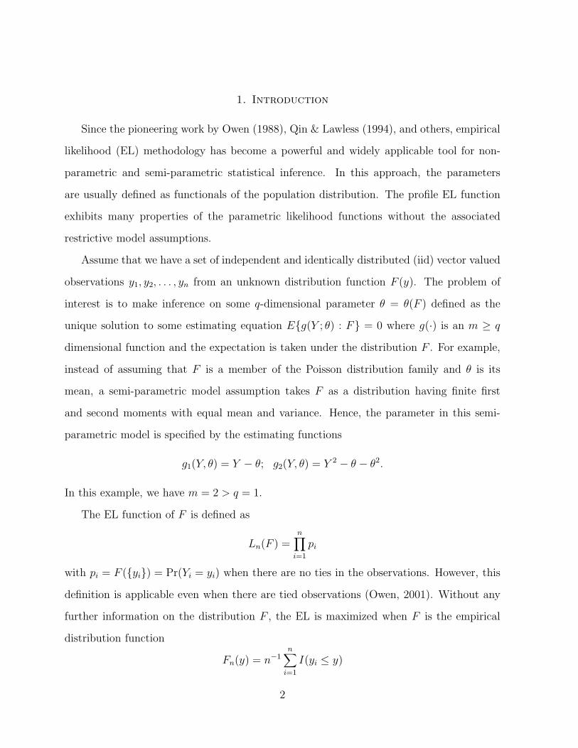
1. Introduction

Since the pioneering work by Owen (1988), Qin & Lawless (1994), and others, empirical

likelihood (EL) methodology has become a powerful and widely applicable tool for non-

parametric and semi-parametric statistical inference. In this approach, the parameters

are usually defined as functionals of the population distribution. The profile EL function

exhibits many properties of the parametric likelihood functions without the associated

restrictive model assumptions.

Assume that we have a set of independent and identically distributed (iid) vector valued

observations y1, y2, . . . , yn from an unknown distribution function F (y). The problem of

interest is to make inference on some q-dimensional parameter θ = θ(F ) defined as the

unique solution to some estimating equation E{g(Y ; θ) : F} = 0 where g(·) is an m ≥ q

dimensional function and the expectation is taken under the distribution F . For example,

instead of assuming that F is a member of the Poisson distribution family and θ is its

mean, a semi-parametric model assumption takes F as a distribution having finite first

and second moments with equal mean and variance. Hence, the parameter in this semi-

parametric model is specified by the estimating functions

g1(Y, θ) = Y − θ; g2(Y, θ) = Y 2 − θ − θ2.

In this example, we have m = 2 > q = 1.

The EL function of F is defined as

Ln(F ) =n

∏

i=1

pi

with pi = F ({yi}) = Pr(Yi = yi) when there are no ties in the observations. However, this

definition is applicable even when there are tied observations (Owen, 2001). Without any

further information on the distribution F , the EL is maximized when F is the empirical

distribution function

Fn(y) = n−1n

∑

i=1

I(yi ≤ y)

2

where I(·) is the indicator function, and the inequality is interpreted componentwise. In

general, it is more convenient to work with the logarithm of the empirical likelihood

ln(F ) =n

∑

i=1

log(pi). (1)

We further require∑n

i=1 pi = 1; see Owen (2001) for justification.

Let θ be defined by the estimating equation E{g(Y ; θ) : F} = 0. In Qin & Lawless

(1994) or Owen (2001), the profile empirical log-likelihood function of θ is defined as

lEL(θ) = sup{ln(F ) : pi ≥ 0, i = 1, . . . , n;n

∑

i=1

pi = 1,n

∑

i=1

pig(yi, θ) = 0}. (2)

When the model is correct and some moment conditions on F are satisfied, the profile

empirical log-likelihood function has many familiar optimalilty properties similar to those

of its parametric sibling. In particular, when θ is defined by g(Y, θ) = Y − θ, the profile

empirical log-likelihood function lEL(θ) can conveniently be used to construct asymptotic

confidence regions for θ. Such confidence regions are valued for their data-driven shape

and range-respecting properties.

To solve the numerical problem related to lEL(θ), a prerequisite is that the convex

hull of {g(yi, θ), i = 1, 2, . . . , n} must have the zero vector as an interior point. In the

simple example of population mean, lEL(θ) is well defined for all θ in the convex hull of

{yi, i = 1, 2, . . . , n}. In applications that we shall discuss in more detail, the dimension m

of g can be much larger than the dimension q of the parameter θ. It can be difficult to

determine the region Θ over which lEL(θ) is well defined. In fact, it is possible that Θ is

empty. A convention is to define lEL(θ) = −∞ for θ 6∈ Θ. However, this strategy has two

drawbacks: (1) It is often difficult to specify the region Θ which is data specific, and (2)

for any pair of θ1, θ2 6∈ Θ, the values lEL(θ1) and lEL(θ2) provide no information on their

relative plausibility, even if one is close to and the other is far away from the boundary of

Θ. In particular, the second drawback makes it a challenge to find the maximum point of

lEL(θ). Even finding a proper initial value can be difficult in this case.

3

In this article, we make a novel adjustment to the commonly used EL. With this ad-

justment, the profile adjusted empirical likelihood (AEL) is well defined for all parameter

values. Hence, it is not necessary to determine whether θ ∈ Θ and consequently finding the

maximum point of the adjusted lEL(θ) becomes much simpler. Further, the new solution

provides a good initial value for θ when Θ is non-empty in the original problem. We also

show that the asymptotic properties of the EL are preserved. The adjusted EL confidence

regions based on the chi-square limiting distribution are always larger. Hence, it has higher

coverage probability particularly when the sample size is small and provides a promising

solution to the small-sample under-coverage problem discussed in Tsao (2004). As will be

seen in our simulation later, the improved coverage probability is achieved without resort-

ing to complex techniques such as Bartlett-correction or bootstrap calibration. In fact, the

algorithm for the AEL converges more quickly than the algorithm for the EL. Finally, a

numerical algorithm for computing the profile AEL is given with guaranteed convergence.

The rest of the article is organized as follows. In Section 2, we give additional details

of EL and its extensions. In Section 3, we introduce our new method. The asymptotic

properties of the new method are discussed in Section 4. In Section 5, we present a simple

algorithm for computing the adjusted profile empirical log-likelihood ratio function. We

demonstrate the usefulness of the new method by simulation and by examples. We draw

several conclusions in Section 6, and two proofs are given in the Appendix.

2. Empirical likelihood

As in the introduction, let y1, y2, . . . , yn be a set of independent and identically dis-

tributed (iid) vector valued observations. Let g(Y, θ) be the estimating function that defines

the parameter θ of the population distribution F through E{g(Y, θ)} = 0. The empirical

log-likelihood ln(F ) is defined by (1) and the profile empirical log-likelihood lEL(θ) is de-

fined as in (2). Let Θ be the set of parameter values such that for each θ ∈ Θ, the solution

4

ton

∑

i=1

pig(yi, θ) = 0 (3)

exists for the pi values. For each θ ∈ Θ, ln(F ) under constraint (3) is maximized when

pi =1

n{1 + λ′g(yi, θ)},

for i = 1, 2, . . . , n with the Lagrange multiplier λ being the solution of

n∑

i=1

pig(yi, θ) = 0.

Hence, we also have the following expression for the profile empirical log-likelihood function,

lEL(θ) = −n log(n) −n

∑

i=1

log{1 + λ′

g(yi, θ)}.

We further define the profile empirical log-likelihood ratio function,

W (θ) =n

∑

i=1

log(npi) = −n

∑

i=1

log{1 + λ′

g(yi, θ)}.

When g(y, θ) = y − θ and θ0 is the true population mean, Owen (1990) shows that

−2W (θ0) → χ2m in distribution as n → ∞ under some moment conditions. This is similar

to the result for parametric likelihood (Wilks, 1938), which is the foundation for the con-

struction of confidence regions and of the hypothesis test on θ. An approximate 100(1−α)%

region is given by

{θ : −2W (θ) ≤ χ2m(1 − α)} (4)

where χ2m(1 − α) is the (1 − α)th quantile of the chi-square distribution with m degrees

of freedom. Unlike the confidence regions constructed via the normal approximation, the

EL regions have data-driven shape, are range respecting, and often have better coverage

properties (Owen, 1990; Chen et al., 2003).

The results for the population mean are more general. Similar conclusions are true

for linear models, generalized linear models, models defined by estimating equations, and

many others (Owen 1991; Kolaczyk 1994; Qin & Lawless 1994). In applications, we must

solve the problem of computing W (θ) at various θ values.

5

3. The constraint problem and the adjustment

Computing W (θ) numerically is usually done by solving

n∑

i=1

g(yi, θ)

1 + λ′g(yi, θ)= 0 (5)

for the Lagrange multiplier λ. We look for a solution λ that satisfies 1 + λ′

g(yi, θ) > 0 for

all i = 1, 2, . . . , n. A necessary and sufficient condition for its existence is that the zero

vector is an interior point of the convex hull of {g(yi, θ), i = 1, 2, . . . , n}.

By definition, the true parameter value θ0 is the unique solution of E{g(Y ; θ) : F} = 0.

Hence, under some moment conditions on g(Y, θ) (Owen, 2001), the convex hull {g(yi, θ0), i =

1, 2, . . . , n} contains 0 as its interior point with probability 1 as n → ∞. When θ is not

close to θ0, or when n is small, there is a good chance that the solution to (5) does not

exist. This can be a serious limitation in some applications as shown in the examples in

the next section. In this section, we propose the following AEL.

Denote gi = gi(θ) = g(yi; θ) and gn = gn(θ) = n−1 ∑ni=1 gi for any given θ. For some

positive constant an, define

gn+1 = gn+1(θ) = −an

n

n∑

i=1

gi = −angn.

We now adjust the profile empirical log-likelihood ratio function to be

W ∗(θ) = sup{n+1∑

i=1

log[(n + 1)pi] : pi ≥ 0, i = 1, . . . , n + 1;n+1∑

i=1

pi = 1;n+1∑

i=1

pigi = 0}. (6)

Since the convex hull of {gi, i = 1, 2, . . . , n, n + 1} for any given θ contains 0, W ∗(θ) is well

defined for all θ.

It can be seen that if gn(θ) = 0, we have W ∗(θ) = W (θ) = 0. For θ values such that

gn ≈ 0, we have W (θ) ≈ W ∗(θ). When θ 6∈ Θ, we have W (θ) = −∞ whereas W ∗(θ) is still

well defined and is likely to assume a negative value with its magnitude depending on how

far θ deviates from Θ. Hence, W ∗(θ) is informative for maximizing W (θ).

6

The value of an should be chosen according to the specific nature of the application. In

theory, the first order asymptotic property of W (θ0) is unchanged for W ∗(θ0) as long as

an = op(n2/3). When an = Op(n

1/2) and θ = θ0, we have gn+1 = Op(1) under mild moment

conditions. Thus, the effect of our adjustment is mild: it is equivalent to adding a few

artificial but comparable observations to the set of n original observations. Nevertheless,

we recommend the use of an with smaller magnitude.

When θ is far from θ0, some gi values can be much larger than the rest of the gi

values. In this case, the gn can substantially deviate from 0 and distort the true likelihood

configuration around θ. When the semi-parametric model is correct, this problem will not

occur if a good initial estimate of θ0 is available. The profile likelihood ratio function will be

low around θ compared to in the neighborhood of θ0. When the model is incorrect, which

occurs in the model selection example in the next section, there will be no hypothetical θ0

to rely on. Our strategy is to replace gn by the median or trimmed mean of the gi. The

particular form of gn can be chosen by the user.

In most applications, the focus is on θ in a small neighborhood of θ0 so that gn is of

moderate size. Our general recommendation is to have an = max(1, log(n)/2) coupled

with a trimmed version of gn when appropriate. Investigation of the optimal choice of an in

various practically important situations is still under way. When the sample size n increases,

our estimate of θ0 will get into its n−1/2 range, hence this an will make angn = op(1).

The effect of the adjustment is well below the order of n−1/2. Yet when n is small, this

adjustment is effective at improving the coverage probability of the confidence regions.

We now give a simple example to illustrate the convex hull problem and the adjustment.

We generate 50 observations from an independent bivariate standard normal distribution.

We compute the profile likelihood at (µ1, µ2) = (2, 2). Figure 1 (left) gives the plot of

g values and it is seen that the convex hull does not contain 0. By adding an artificial

observation gn+1 = −angn with an = log(n)/2, the convex hull is expanded and 0 is now

7

an interior point as in Figure 1 (right). Since (2, 2) is well outside of the convex hull, the

adjustment in this case appears to be substantial. However, the empirical log-likelihood is

merely adjusted from −∞ to some large negative finite number, and this does not really

have a large impact. At the same time, one will not notice anything substantial in the

adjustment of EL at (µ1, µ2) = (0, 0).

−4 −2 0 2 4

−4

−2

02

4

g1

g2

−4 −2 0 2 4

−4

−2

02

4

g1

g2

Figure 1: Convex hull (left) and adjusted convex hull with an = log(n)/2 (right). The bold

dot is (0,0).

4. Asymptotic properties

The most important result in the context of EL is the limiting distribution of the em-

pirical log-likelihood ratio function at θ0. We show that the AEL has the same asymptotic

properties as the unadjusted EL.

Theorem 1 Let y1, y2, . . . , yn be a set of independent and identically distributed vector ob-

servations of dimension q from some unknown distribution F0. Let θ0 be the true parameter

that satisfies E{g(Y, θ) : F0} = 0 where g is a vector valued function with dimension m.

Assume further that Var{g(Y, θ) : F0} is finite and has rank m > q. Let W ∗(θ) be the

8

adjusted profile empirical log-likelihood ratio function defined by (6) and an = op(n2/3). As

n → ∞, we have

−2W ∗(θ0) → χ2m

in distribution.

Proof: See Appendix.

If the rank of Var{g(Y, θ) : F0} is lower than m, then some components of the estimating

function g can be removed from the constraint set and the foregoing conclusion can be

revised accordingly. This result can be compared to Theorem 3.4 in Owen (2001). Based

on this result, an empirical-likelihood-based confidence interval (region) as discussed in the

introduction can be easily constructed. When θ is the population mean, the confidence

regions using AEL are no longer confined within the convex hull of the observed values.

Thus, the new method has the potential to effectively improve the under-coverage problem

due to small sample size or high dimension.

We are naturally interested in knowing the asymptotic behavior of W ∗(θ) and W (θ)

when θ 6= θ0. Interestingly, this problem has not received much attention in the literature.

Theorem 2 Assume that the conditions in Theorem 1 hold and that for some θ 6= θ0

‖E{g(Y, θ)}‖ > 0.

Then, −2n−1/3W ∗(θ) → ∞ and −2n−1/3W (θ) → ∞ in probability as n → ∞.

The proof of Theorem 2 is also given in the Appendix. Based on Theorems 1 and

2, it is easily seen that the non-parametric maximum empirical likelihood estimator is

consistent with some minor additional conditions. In addition, when θ is not the true

value, the empirical likelihood ratio statistic tends to infinity at the rate of at least n1/3.

Qin & Lawless (1994) showed that there exists a local maximum of W (θ) in an n−1/3

neighborhood of θ0. The same is true for W ∗(θ). Because the proofs of this and other

results do not contain new techniques, we present only one result here.

9

Theorem 3 Assume that the conditions in Theorem 1 hold, and that ∂2g(y, θ)/(∂θ∂θ′

) is

continuous in the neighborhood of θ0. Also assume that ‖g(y, θ)‖3 and ‖∂2g(y, θ)/(∂θ∂θ′

)‖

are bounded by some integral function G(y) in the neighborhood of θ0. Let θ be a local

maximum of W ∗(θ) in an n−1/3 neighborhood of θ0. As n → ∞, we have

√n(θ − θ0) → N(0, Σ)

in distribution, where

Σ = {E(∂g/∂θ)′

(Egg′

)−1 E(∂g/∂θ)}−1.

5. Numerical algorithm, simulations, and examples

Since the constraints in the AEL are always satisfied, the numerical computation of the

profile AEL can be done with any existing algorithm. In particular, we recommend the

modified Newton-Raphson algorithm proposed by Chen et al. (2002). To maximize W ∗(θ)

with respect to θ, we use the simplex method introduced by Nelder & Mead (1965) for the

sake of its stability. Most optimization software includes a built-in function for the simplex

method.

For given θ and an, we compute W ∗(θ) as described in the following pseudo-code:

1. Compute gi = g(yi, θ) for i = 1, . . . , n and gn+1 = −angn. The sample mean gn may

be replaced by a trimmed mean or any other robust substitute.

2. Set the initial value for the Lagrange multiplier λ0 = 0. Initialize iteration number

k = 0, and let γ = 1 and ε = 10−8 be the step size in the iteration and the tolerance

level respectively.

3. Compute the first and second partial derivatives of

R(λ) =n+1∑

i=1

log(1 + λ′

gi)

10

with respect to λ evaluated at λk. Let these be R and R and further compute

∆ = −R−1R.

If ‖∆‖ < ε stop the iteration, report λk, and go to Step 6.

4. Compute δ = γ∆. If any 1 + (λk + δ)′

gi ≤ 0 or R(λk + δ) < R(λk), let γ = γ/2, and

repeat this step. Otherwise, continue to the next step.

5. Let λk+1 = λk − δ and γ = (k + 1)−1/2. Increase the count k by 1. Return to Step 3.

6. Report λk and the value of W ∗(θ) = −∑n+1i=1 log(1 + λkgi).

The convergence of the iteration is guaranteed because the existence of a solution is

assured. We refer to Chen et al. (2002) for the proof of the algorithmic convergence. The

foregoing operations result in the value of W ∗(θ). We then use the simplex method to

optimize this function. A set of good initial values of θ will be helpful in this step. In

general, one may use a rough estimate of θ such as via the method of moments. We

demonstrate the usefulness of AEL in the following examples.

5.1. Confidence region

Constructing confidence regions for the population means received primary attention in the

pioneering paper of Owen (1988). The empirical likelihood confidence regions have data-

driven shape, are range respecting, and are Bartlett-correctable (DiCiccio et al., 1991).

When the sample size is not large, one may replace chi-square distribution calibration by

bootstrap calibration to improve the accuracy of the coverage probability. As discussed in

Tsao (2004), however, confidence regions computed via the unadjusted EL are by definition

confined to be inside the convex hull formed by the observed values, which is not affected

by Bartlett correction or by bootstrap calibration. When the sample size is small, even the

convex hull may not have a large enough coverage probability. In comparison, W ∗(θ) is

11

finite for all θ. Thus, the confidence regions are no longer confined to be within the convex

hull of the data. It is hence better suited to solve the under-coverage problem.

For illustration, we applied the new method to construct confidence intervals for the

examples discussed in DiCiccio et al. (1991). We used their settings. The coverage prob-

abilities are based on 5000 simulations. The data were drawn from the standard normal

distribution with sample sizes 10 and 20, a χ2(1) distribution with sample sizes 20 and 40,

and a t(5) distribution with sample sizes 15 and 30. We let an = log(n)/2 in the definition of

gn+1. We reproduce the Bartlett-correction results from DiCiccio et al. (1991) for compar-

ison. The coverage probabilities of intervals based on unadjusted EL, Bartlett-corrected,

and AEL are given in Table 1 for nominal levels of 80, 90, 95, and 99 percent. It is clear that

the coverage probabilities of the AEL are closer to the target values for the sample sizes and

population distributions considered. The results are particularly impressive since the AEL

does not involve complex theory or computational procedures. We also conducted simula-

tions with relatively large sample sizes (n = 100, 200, 500), and the coverage probabilities

were close to the target values for all methods.

We simulated the coverage probabilities of a bivariate population mean. We repeated the

simulation 5000 times with an = log(n)/2 for bivariate distributions: (1) two independent

standard normal distributions, (2) two independent χ2(1) distributions, (3) two independent

t(5) distributions. The coverage probabilities are reported in Table 2. It is clear that the

AEL compares favorably with the usual unadjusted EL. The coverage probabilities are

substantially improved with the AEL method. Our simulations also revealed that the AEL

is computationally simpler: the time taken was only about one-fifth to one-seventh of the

time for the unadjusted EL.

To provide a more concrete comparison between the confidence regions constructed with

the unadjusted and the adjusted EL, we considered a data set given in Owen (2001, p. 31).

The original source of this data set is Iles (1993). It consists of four types of prey (Caddis fly

12

Table 1: Coverage Probabilities of Population Mean

Normal Data

n = 10 n = 20

NV 0.80 0.90 0.95 0.99 0.80 0.90 0.95 0.99

EL 0.7396 0.8318 0.8940 0.9526 0.7802 0.8756 0.9284 0.9794

TB 0.7796 0.8706 0.9182 0.9650 0.8006 0.8962 0.9416 0.9844

EB 0.7938 0.8802 0.9246 0.9696 0.8034 0.8980 0.9424 0.9848

AEL 0.7964 0.8892 0.9444 0.9962 0.8138 0.9028 0.9522 0.9898

χ2(1) Data

n = 20 n = 40

EL 0.7332 0.8354 0.8928 0.9524 0.7682 0.8640 0.9170 0.9742

TB 0.7872 0.8772 0.9262 0.9706 0.7910 0.8896 0.9418 0.9800

EB 0.7634 0.8546 0.9034 0.9616 0.7804 0.8789 0.9334 0.9774

AEL 0.7714 0.8652 0.9168 0.9660 0.7930 0.8810 0.9330 0.9818

t(5) Data

n = 15 n = 30

EL 0.7544 0.8504 0.9098 0.9674 0.7784 0.8834 0.9338 0.9812

TB 0.8266 0.9106 0.9544 0.9862 0.8114 0.9042 0.9496 0.9866

EB 0.7898 0.8884 0.9348 0.9794 0.7954 0.8928 0.94222 0.9832

AEL 0.7986 0.8944 0.9418 0.9876 0.8098 0.9070 0.9500 0.9874

NV = nominal value; EL = empirical likelihood; TB = EL with theoretical Bartlett correction;

EB = EL with estimated Bartlett correction; AEL = Adjusted EL.

13

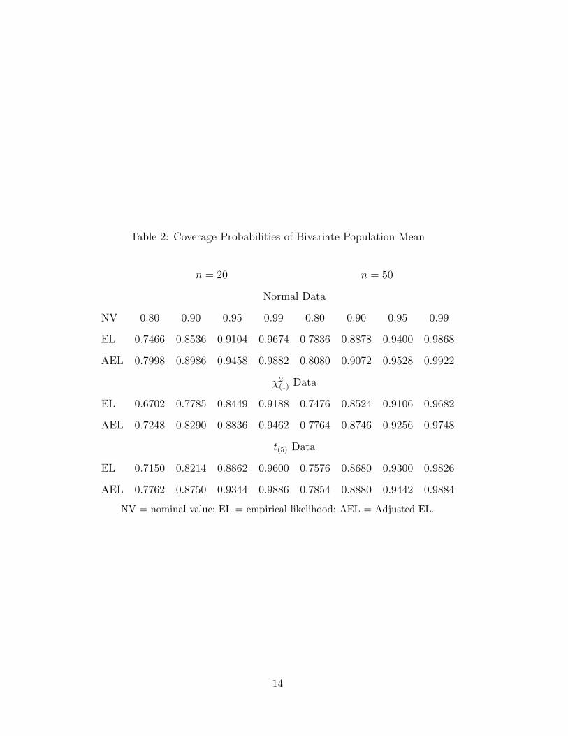
Table 2: Coverage Probabilities of Bivariate Population Mean

n = 20 n = 50

Normal Data

NV 0.80 0.90 0.95 0.99 0.80 0.90 0.95 0.99

EL 0.7466 0.8536 0.9104 0.9674 0.7836 0.8878 0.9400 0.9868

AEL 0.7998 0.8986 0.9458 0.9882 0.8080 0.9072 0.9528 0.9922

χ2(1) Data

EL 0.6702 0.7785 0.8449 0.9188 0.7476 0.8524 0.9106 0.9682

AEL 0.7248 0.8290 0.8836 0.9462 0.7764 0.8746 0.9256 0.9748

t(5) Data

EL 0.7150 0.8214 0.8862 0.9600 0.7576 0.8680 0.9300 0.9826

AEL 0.7762 0.8750 0.9344 0.9886 0.7854 0.8880 0.9442 0.9884

NV = nominal value; EL = empirical likelihood; AEL = Adjusted EL.

14

0 50 100 150 200 250 300 350 4000

100

200

300

400

500

600

700

800

900

Caddis fly larvae

Sto

nefly

larv

e

EL

AEL

0 100 200 300 400 500 600 700 800 900 10000

100

200

300

400

500

600

700

800

900

Mayfly larvae

Oth

er in

vert

ebra

tes

AEL

EL

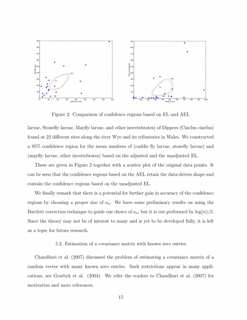
Figure 2: Comparison of confidence regions based on EL and AEL

larvae, Stonefly larvae, Mayfly larvae, and other invertebrates) of Dippers (Cinclus cinclus)

found at 22 different sites along the river Wye and its tributaries in Wales. We constructed

a 95% confidence region for the mean numbers of (caddis fly larvae, stonefly larvae) and

(mayfly larvae, other invertebrates) based on the adjusted and the unadjusted EL.

These are given in Figure 2 together with a scatter plot of the original data points. It

can be seen that the confidence regions based on the AEL retain the data-driven shape and

contain the confidence regions based on the unadjusted EL.

We finally remark that there is a potential for further gain in accuracy of the confidence

regions by choosing a proper size of an. We have some preliminary results on using the

Bartlett correction technique to guide our choice of an, but it is out-performed by log(n)/2.

Since the theory may not be of interest to many and is yet to be developed fully, it is left

as a topic for future research.

5.2. Estimation of a covariance matrix with known zero entries

Chaudhuri et al. (2007) discussed the problem of estimating a covariance matrix of a

random vector with many known zero entries. Such restrictions appear in many appli-

cations, see Grzebyk et al. (2004). We refer the readers to Chaudhuri et al. (2007) for

motivation and more references.

15

Suppose we have a random vector Y = (Y1, Y2, Y3, Y4)′

whose covariance matrix Σ has

the form

Σ =

σ11 0 σ13 0

0 σ22 0 σ24

σ13 0 σ33 σ34

0 σ24 σ34 σ44

.

Under the normality assumption, both the mean µ = E{Y } and the covariance matrix can

be estimated by the maximum likelihood estimator. However, maximizing the likelihood

function under the constraint of some covariances being zero is not a simple problem.

Chaudhuri et al. (2007) presented many numerical algorithms for this problem. One method

is to ignore the normality assumption and to use EL instead. Let yij, i = 1, . . . , n and

j = 1, 2, 3, 4 be a set of n observations from a distribution F with mean µ and covariance

matrix Σ. Chaudhuri et al. (2007) proposed computing the profile EL at a given feasible µ

and Σ:

lEL(µ, Σ) = sup{n

∑

i=1

log pi : pi > 0;n

∑

i=1

pi = 1;n

∑

i=1

pi(yij − µj) = 0;

n∑

i=1

pi(yij − µj)(yjk − µk) = 0; (j, k) = (1, 2), (1, 4), (2, 3)}.

The maximum empirical likelihood estimates of µ and Σ are taken as the maximum points

of lEL(µ, Σ). It was found that when the normal model is true, the maximum empirical

likelihood estimator has almost the same efficiency as the parametric maximum likelihood

estimator. When normality is violated, the maximum empirical likelihood estimator is

more efficient.

When the sample size is small (n = 10), Chaudhuri et al. (2007) experienced prob-

lems with the EL procedure due to an inability to find feasible starting values. With the

AEL, however, this problem disappears immediately. According to our own simulation,

the minimizer of W ∗(µ, Σ) (with an = n−1) provides excellent initial values for maximizing

lEL(µ, Σ). We used an = n−1 instead of an = max{1, log n/2} to better approximate the

16

solution of lEL(µ, Σ). Interestingly, the minimizer of W ∗(µ, Σ) itself serves as an efficient

estimator when an = n−1. The best choice of an in terms of efficiency is beyond the scope

of this article. The following simulation study demonstrates that the AEL provides good

initial values and more efficient estimation.

We simulated data sets Y = (Y1, Y2, Y3, Y4)′

from a multivariate normal distribution

with zero mean vector and covariance matrix Σ

Σ =

1 0 0.375 0

0 1 0 0.165

0.375 0 1 0.65

0 0.165 0.65 1

.

We let the sample size n = 10 and generated 1000 sets of random samples from the normal

model. By using the sample mean as the initial value for µ, we failed to find a solution for

the linear constraints in 75.9% of the samples. We next computed the AEL with an = n−1

where the existence of the solutions is guaranteed. The maximum AEL mean estimator

was then used to provide an initial value for the unadjusted EL. This time, we failed to

find a solution in only 17.4% of the samples. Thus, the AEL is useful as an initial-value

locator even if one insists on using the original EL.

Further, we are interested in the efficiency of the maximum AEL estimator itself. We

computed the total bias and root mean square error (RMSE) of the maximum unadjusted

and adjusted EL estimates according to the following definitions:

Total bias =∑

i<j

| 1

M

M∑

k=1

(σ(k)ij − σij)|

and

RMSE =

√

√

√

√

√

∑

i<j

1

M

M∑

k=1

(σ(k)ij − σij)2

where σ(k)ij is the estimate of σij in the kth simulation data set and M is the total number of

simulations. For this comparison, we set n = 20 and the number of simulations M = 10000.

17

For the unadjusted EL, we did not find solutions in 2.1% of the simulations. Hence, total

bias and root mean square error were computed based on the remaining 97.9% of the

samples.

The bias of the maximum unadjusted and the adjusted EL estimators for the standard

deviations were found to be 0.98 and 1.00. Clearly, these two methods have similar bias

properties. The RMSEs for the maximum unadjusted and adjusted EL were found to be

0.87 and 0.81 which implies that the AEL method has about a 13% gain in efficiency.

We should certainly be cautious in generalizing this conclusion and more studies will be

needed. The key advantage of the adjusted EL method in this example is computational;

the solution is guaranteed to exist.

In most applications, having a sample size as small as n = 10 may be unusual. However,

when the dimension of y increases, the problem of finding feasible starting values can remain

a serious challenge even for moderate to large sample sizes. Our method can be used both

to search for feasible starting values and to directly provide efficient estimates of unknown

parameters in this and similar applications. The best choice of an to achieve the highest

efficiency is beyond the scope of this article.

5.3. Variable selection in regression analysis

Assume that we have n independent observations described by the following linear

model

yi = β0 + x′

iβ + ǫi

i = 1, 2, . . . , n such that ǫi are independent errors with mean 0 and finite nonzero variance

σ2. We denote the dimension of x as m. In applications, the covariate xi has high dimension

and not all components of the regression coefficient β are meaningfully different from 0.

Thus, a variable selection step is often applied to reduce the complexity of the model and

hence reduce the variability in the estimators.

18

There are many well-known variable selection procedures. The Akaike information

criterion (AIC) and the Bayes information criterion (BIC) are among the most investigated

methods in the literature (Akaike, 1973; Schwarz, 1978; Shao, 1997). Both criteria choose

a model specified by a subset of covariates by their penalized likelihood values. In general,

a parametric distributional assumption for ǫ is required.

To avoid the parametric assumption, Kolaczyk (1994) and Mulayath (2006) discussed

the empirical-likelihood-based information criteria. Assume that we have a set of indepen-

dent observations as given earlier. Let s be a subset of indices of covariate variables. We use

xi[s] and β[s] to denote the corresponding subset of covariates and regression coefficients.

For each given s, the profile EL is given by

lEL(β0, β[s], σ2) = sup

{

n∑

i=1

log pi : pi > 0;n

∑

i=1

pi = 1;n

∑

i=1

pi(yi − β0 − x′

i[s]β[s]) = 0;

n∑

i=1

pix′

i(yi − β0 − x′

i[s]β[s]) = 0.

}

.

Note that the number of constraints remains a constant with respect to s in the definition

of the profile likelihood. This is important for differentiating the plausibility of submodels

formed by a subset of covariates.

The profile empirical likelihood ratio function W (β0, β[s], σ2) is similarly defined. For

convenience, we shall omit the entries of β0 and σ2 in this notation. The empirical-

likelihood-based Akaike information criterion

EAIC(s) = 2 inf{W (β[s]) : β0, β[s], σ2} + 2k

with k being the number of covariates in s. We choose the submodel corresponding to the

s that minimizes EAIC(s). Similarly, we define

EBIC(s) = 2 inf{W (β[s]) : β0, β[s], σ2} + k log n.

This empirical version of BIC chooses the submodel s that minimizes EBIC(s).

19

We refer to Kolaczyk (1994) and Mulayath (2006) for specific discussion of the properties

of EAIC and EBIC for variable selection. Before these methods can be used, one must make

sure that both EAIC and EBIC are well defined.

Consider the most extreme case where s is empty, but the dimension of x (i.e., m) is

relatively large while n is not so large. In this case, the constraints imply that we must

find a value of β0 such that

n∑

i=1

pi = 1;

n∑

i=1

pi(yi − β0) = 0;

n∑

i=1

pix′

i(yi − β0) = 0

have solutions in the pi values. In the special case where yi = xi and m = 1, this implies that

β20 = (

∑

pixi)2 =

∑

pix2i . This is possible only if pi degenerates which implies EAIC(s) =

EBIC(s) = ∞. With the AEL, the solution exists for any choice of β0. Thus, sensible and

informative values of EAIC(s) and EBIC(s) are always defined after the adjustment and

can be easily computed. We choose an = log(n)/2 because it worked well for constructing

confidence regions. Yet the key in this application is to guarantee that the optimization

problem has a solution for any candidate model of interest. Hence, the size of an is not of

particular importance.

We now consider the cancer study example given by Stamey et. al (1989) for the variable

selection problem. This study examines the correlation between the levels of prostate spe-

cific antigen (PSA) and 8 clinical measurements of 97 men who were yet to receive a radical

prostatectomy. The clinical measurements considered here for the multiple linear regres-

sion of log(PSA) are logarithm of cancer volume (lcavol), logarithm of weight (lweight),

age, logarithm of benign prostate hyperplasia amount (lbph), seminal vesicle invasion (svi),

logarithm of capsular penetration (lcp), Gleason score (gleason), and percentage of Gleason

score 4 or 5 (pgg45). The aim of this analysis is to predict the logarithm of PSA based

20

Table 3: Variable Selection Problem - Prostate Cancer Data

Variables OLS AIC EAIC/BIC/EBIC

Intercept 0.6694 (1.2963) 0.1456(0.5975) -0.2681(0.5435)

lcavol 0.5870(0.0879) 0.54860.0741) 0.5516(0.0747)

lweight 0.4545(0.1700) 0.3909(0.1660) 0.5085(0.1502)

age -0.0196(0.0112) - -

lbph 0.1071(0.0584) 0.0901(0.0562) -

svi 0.7662(0.2443) 0.7117(0.2100) 0.6662(0.2098)

lcp -0.1055(0.0910) - -

gleason 0.0451(0.1575) - -

pgg45 0.0045(0.0044) - -

on the 8 covariates. We apply variable selection methods AIC, BIC, EAIC, and EBIC to

identify the appropriate model. Defining the submodels by setting the regression coeffi-

cients to zero for all covariates not in the submodel, we face computational issues due to

the non-existence of a solution to the equation∑n

i=1 pig(yi, xi, β) = 0 for given β. The AEL

works well in this example. Covariates lcavol, lweight, and svi were identified to form an

appropriate model by EAIC, BIC, and EBIC whereas the model identified by AIC includes

an additional variable lbph. These models, the estimates of the corresponding regression

parameters, the estimates of standard errors (in brackets), and the ordinary least square

(OLS) estimates based on the full model are given in Table 3. We can see that all the

methods pick up the most significant covariates. The AIC picks a slightly larger model

than EAIC does.

6. Conclusions

In this article, we suggested a method to overcome the difficulty posed by the non-

21

existence of solutions while computing the profile empirical likelihood. We demonstrated

that the proposed AEL is well defined for all parameter values. The new method sub-

stantially enhances the applicability of EL. We showed that the resulting AEL retains the

asymptotic optimality properties. Further, the confidence regions constructed by the new

method have closer to nominal coverage probabilities in the examples considered. The al-

gorithm associated with the AEL also converges much faster, reducing the computational

burden. The usefulness of this new method was illustrated via a number of examples.

Acknowledgments

This research is support by the Natural Science and Engineering Research Council of

Canada and by the MITACS. The authors thank the Editor, Associate Editor and referees

for helpful comments.

Appendix

Because the proofs of some similar results are well known and can be easily found in

Owen (2001), our proofs here will be brief and somewhat simplistic.

Proof of Theorem 1:

Let the eigenvalues of Var{g(Y, θ0)} be σ21 ≤ σ2

2 ≤ · · · ≤ σ2m. Without loss of generality,

we assume that σ21 = 1. Let λ be the solution to

n+1∑

i=1

gi

1 + λ′gi

= 0. (7)

We first show that λ = Op(n−1/2). For brevity, we claim that λ = op(1) which is easy to

verify. Our task is to refine this assessment.

Let g∗ = max1≤i≤n ‖gi‖. The moment assumption implies that

g∗ = op(n1/2) and gn = Op(n

−1/2).

22

Let ρ = ‖λ‖ and λ = λ/ρ. Multiplying n−1λ′

to both sides of (7), we get

0 =λ

′

n

n+1∑

i=1

gi

(1 + λ′gi)

=λ

′

n

n+1∑

i=1

gi − ρn+1∑

i=1

(λ′

gi)2

(1 + ρλ′gi)

≤ λ′

gn(1 − an/n) − ρ

n(1 + ρg∗)n

∑

i=1

(λ′

gi)2

= λ′

gn − ρ

n(1 + ρg∗)n

∑

i=1

(λ′

gi)2 + Op(n

−3/2an). (8)

The inequality above is valid because the (n + 1)th term of the second summation is non-

negative. Consequently, the variance assumption on V ar{g(Y, θ0)} implies that

n−1n

∑

i=1

(λ′

gi)2 ≥ (1 − ǫ)σ2

1 = 1 − ǫ

in probability for some 1 > ǫ > 0. Therefore, as long as an = op(n), (8) implies that

ρ

(1 + ρg∗) ≤ λ′

gn × (1 − ǫ)−1 = Op(n−1/2)

which further implies that ρ = Op(n−1/2) and hence λ = Op(n

−1/2).

Next, denoting Vn = n−1 ∑ni=1 g

′

igi, we find that

0 =1

n

n+1∑

i=1

gi

1 + λ′gi

= gn − λ′

Vn + op(n−1/2).

Hence, when n → ∞, λ = V −1n gn + op(n

−1/2).

Finally, we expand W ∗ as follows.

−2W ∗(θ0) = 2n+1∑

i=1

log(1 + λ′

gi)

= 2n+1∑

i=1

{λ′

gi − (λ′

gi)2/2} + op(1).

Substituting the expansion of λ, we get that

−2W ∗(θ0) = ng′

nV −1n gn + op(1)

23

which converges to a chi-square distribution with m degrees of freedom as n → ∞.

Remark: When gn is replaced by any other Op(n−1/2) random quantity in the definition

of gn+1, the foregoing proof still goes through with no changes. Even if an has larger order

such that an = op(n), the proof still works. The assumption of an = op(n2/3) makes the

next proof simpler. Using a large an in most cases is not advisable.

Proof of Theorem 2:

Note again that gi = g(yi, θ), i = 1, . . . , n and similarly define gn and gn+1. By the law

of large numbers, as n → ∞, ‖g′

ngn‖ → δ2 > 0 in probability. Note that gi − gn has mean

zero, and satisfies all moment conditions to ensure that

max{‖gi − g‖} = op(n1/2).

Let λ = n−2/3gM for some positive constant M . Hence, we have

max{|λ′

gi|, i = 1, . . . , n, n + 1} = op(1).

Thus, with probability going to one, 1 + λ′

gi > 0 for all i = 1, . . . , n, n + 1. Using the

duality of the maximization problem, we find that

W ∗(θ) = − supλ{

n+1∑

i=1

log(1 + λ′

gi)}

≤ −n+1∑

i=1

log(1 + λ′

gi)

= −n1/3δ2M + op(1).

Since M can be arbitrarily large, we have −2n−1/3W ∗(θ) → ∞ for any θ 6= θ0.

The proof of −2n−1/3W (θ) → ∞ is similar.

Remark: First, the sample mean gn can again be replaced by the sample median or

trimmed means without invalidating the foregoing proof. Second, the order of W ∗(θ)

tending to infinity is clearly higher than n1/3. Since the result is useful mostly for obtaining

asymptotic properties of other procedures, the exact order is not of great interest here.

References

24

Akaike, H. (1973), “Information theory as an extension of the maximum likelihood prin-

ciple,” In Petrov, B. N. & Csaki, F. (eds.) Second International Symposium on

Information Theory, Akademiai Kiado, Budapest, 267-282.

Chaudhuri, S., Drton, M., & Richardson, T. S. (2007), “Estimation of a covariance

matrix with zeros,” Biometrika, To appear.

Chen, J., Chen, S., & Rao, J. N. K. (2003), “Empirical likelihood confidence intervals

for a population containing many zero values,” Canadian Journal of Statistics, 31,

53-67.

Chen, J., Sitter, R. R., & Wu, C. (2002), “Using empirical likelihood methods to

obtain range restricted weights in regression estimators for surveys,” Biometrika, 89,

230-237.

DiCiccio, T., Hall, P., & Romano, J. (1991), “Empirical likelihood is Bartlett-

correctable,” The Annals of Statistics, 19, 1053-1061.

Grzebyk, M., Wild, P., & Chouaniere, D. (2004), “On identification of multi-factor

models with correlated residuals,” Biometrika, 91, 141-151.

Iles, T. C. (1993), “Multiple regression,” in J. C. Fry, ed., Biological Data Analysis: A

Practical Approach, Oxford University Press, Oxford, 127-172.

Kolaczyk, E. D. (1994), “Empirical likelihood for generalized linear models,” Statistica

Sinica, 4, 199-218.

Mulayath Variyath, A. (2006), “Variable selection in generalized linear models by

empirical likelihood,” Ph.D. Thesis, Department of Statistics and Actuarial Science,

University of Waterloo. Waterloo, Ontario, Canada.

25

Nelder, J. A. & Mead, R. (1965), “A simplex method for function minimization,”

Computer Journal, 7, 308-313.

Owen, A. B. (1988), “Empirical likelihood ratio confidence interval for a single func-

tional,” Biometrika, 75, 237-249.

Owen, A. B. (1990), “Empirical likelihood confidence regions,” The Annals of Statistics,

18, 90-120.

Owen, A. B. (1991), “Empirical likelihood for linear models,” The Annals of Statistics,

19, 1725-1747.

Owen, A. B. (2001), Empirical Likelihood. Chapman & Hall/CRC, New York.

Qin, J. & Lawless, J. (1994), “Empirical likelihood and general estimating equations,”

The Annals of Statistics, 22, 300-325.

Schwarz, G. (1978), “Estimating the dimension of a model,” The Annals of Statistics,

6, 461-464.

Shao, J. (1997), “An asymptotic theory for linear model selection,” Statistica Sinica, 7,

221-264.

Stamey, T., Kabalin, J., McNeal, J., Johnstone, I., Freiha, F., Redwine,

R., & Yang, N. (1989), “Prostate specific antigen in the diagnosis and treatment of

adenocarcinoma of the prostate II: Radical prostatectomy treated patients,” Journal

of Urology, 16, 1076-1083.

Tsao, M. (2004), “Bounds on coverage probabilities of the empirical likelihood ratio

confidence regions,” The Annals of Statistics, 32, 1215-1221.

Wilks, S. S. (1938), “The large sample distribution of the likelihood ratio for testing

composite hypotheses,” The Annuals of Mathematical Statistics, 9, 60-62.

26