On the Second Order Properties of Empirical

Likelihood with Moment Restrictions

Song Xi Chena∗ and Hengjian Cuib

a∗ Department of Statistics, Iowa State University

Ames, IA 50011-1210, USA

b Department of Mathematics, Beijing Normal University

Beijing, 100875, China

Summary This paper considers the second order properties of empirical likelihood for a

parameter defined by moment restrictions, which is the framework operated upon by the

Generalized Method of Moments. It is shown that the empirical likelihood defined for this

general framework still admits the delicate second order property of Bartlett correction,

which represents a substantial extension of all the established cases of Bartlett correction

for the empirical likelihood. An empirical Bartlett correction is proposed, which is shown to

work effectively in improving the coverage accuracy of confidence regions for the parameter.

Keywords: Bartlett correction, Coverage accuracy, Empirical likelihood, Generalized Method

of Moments.

Running Title: Empirical Likelihood with Moment Restrictions.

1

1. Introduction

Generalized Method of Moments (GMM) introduced by Hansen (1982) is an important

inferential framework in econometric studies. GMM is based on, upon given a model, some

known functions g(X, θ) of a random observation X ∈ Rd and an unknown parameter θ ∈ Rp,

where g : Rd+p → Rr, such that Eg(X, θ) = 0 which constitutes moment restrictions on

the relationship between X and θ. The power of GMM is in its allowing r ≥ p, namely the

number of moment restrictions (instruments) can be larger than the number of parameter,

which leads to a full exploration of inference opportunities provided by the given model.

There is a vast pool of literatures on GMM. Here we only cite the latest reviews of Andrews

(2002), Brown and Newey (2002), Imbens (2002) and Hansen and West (2002).

Empirical likelihood (EL) introduced by Owen (1988) is a computer-intensive statistical

method that facilitates a likelihood-type inference in a nonparametric or semiparametric set-

ting. It is closely connected to the bootstrap as the EL effectively carries out the resampling

implicitly. On certain aspects of inference, EL is more attractive than the bootstrap, for

instance its ability of internal studentizing so as to avoid explicit variance estimation and

producing confidence regions with natural shape and orientation; see Owen (2001) for an

overview of EL. A key property of EL is that the log EL ratio is asymptotically chi-squared

distributed, which resembles the Wilks’ theorem in parametric likelihood. The Wilks’ theo-

rem was established in the original proposal of Owen (1988) for the means, in Hall and La

Scala (1990) for smoothed function of means, Qin and Lawless (1994) for parameters defined

by moment restrictions and Kitamura (1997) for weakly dependence observations.

There have been comprehensive studies of EL in the context of GMM in econometrics.

Imbens (1997) shows that the maximum EL estimator of θ is a one-step variation of the two-

stage GMM estimator in the over-identified case of r > p, and achieves the same asymptotic

efficiency as the two-stage estimator. Testing is considered in Kitamura (2001) for moments

restrictions, and Tripathi and Kitamura (2002) for conditional moment restrictions. Es-

timation and testing with conditional moment restrictions are studied in Donald, Imbens

2

and Newey (2003) and Kitamura, Tripathi and Ahn (2002). They found that EL posses

the attractive features of avoiding estimating optimal instruments and achieving asymptotic

pivotalness. Tilted EL and other variations are studied in Kitamura and Stutzer (1997),

Smith (1997) and Newey and Smith (2004). In particular, Newey and Smith (2004) find

that the EL estimator is favorable in terms of the bias and the second order variance in

comparison with the GMM estimator.

Another key property of the EL is Bartlett correction, which is a delicate second order

property implying that a simple mean adjustment to the likelihood ratio can improve the

approximation to the limiting chi-square distribution by one order of magnitude and hence

can be used to enhance the coverage accuracy of likelihood-based confidence regions. In the

context of testing hypotheses, the Bartlett correction reduces the errors between the nominal

and actual significant levels of an EL test. Bartlett correction has been established for EL

by DiCiccio, Hall and Romano (1991) for smoothed functions of means and Chen (1993,

1994) for linear regression. Baggerly (1998) shows that EL is the only member within the

Cressie-Read power divergence family that is Bartlett correctable. Jing and Wood (1996)

reveal that the exponentially tilted EL for the means is not Bartlett correction as the tilting

alters the delicate second order mechanism of EL.

In this paper we show that the EL with moment restrictions is Bartlett correctable. The

finding represents a substantial extension of all the established cases of Bartlett correction,

which all assume r = p corresponding to the just-identified case in GMM. The establishment

of the Bartlett correction for the just-identified case is a lot easier as the log maximum

EL takes a constant value −n log(n) (n is the sample size). However, in the over-identified

case the maximum EL is no longer a constant, rather it introduces many extra terms into

the log EL ratio and makes the study of Bartlett correction far more challenging as can be

seen from the analysis carried out in this paper. The establishment of Bartlett correction

in this general case indicates that EL inherits the delicate second order mechanism of the

parametric likelihood in a much wider situation. This together with the findings of Imbens

3

(1997), Kitamura (2001) and Newey and Smith (2004) and others suggests that the EL is

an attractive inferential tool in the context of moment restrictions. The establishment of

the Bartlett correction leads to a practical Bartlett correction, which is confirmed to work

effectively for coverage restoration in our simulation studies reported in Section 4.

The paper is organized as follows. Section 2 provides an expansion for the log EL ra-

tio for parameters defined by moment restrictions. Bartlett correction and coverage errors

assessment of EL confidence regions are investigated in Section 3. Simulation results are

reported in Section 4, followed by a general discussion in Section 5. All technical details are

left in the appendix.

2. EL for generalized moment restrictions

Let X1,X2, · · · ,Xn be d−dimensional independent and identically distributed random

sample whose distribution depends on a p−dimensional parameter θ which takes values in

a compact parameter space Θ ⊆ Rp. The information about θ is summarized in the form of

r ≥ p unbiased moment restrictions gj(x, θ), j = 1, 2, · · · , r, such that E[gj(X1, θ0)] = 0 for

a unique θ0, which is the true value of θ. Let

g(X, θ) = (g1(X, θ), g2(X, θ), · · · , gr(X, θ))T and V = V arg(X1, θ0).

We assume the following regularity conditions:

(i) V is a r × r positive definite matrix and the rank of E[∂g(X1, θ0)/∂θ] is p;(2.1)

(ii) For any j, 1 ≤ j ≤ p, all the partial derivatives of gj(x, θ) up to the third order

with respect to θ are continuous in a neighborhood of θ0 and are bounded by some

integrable functions respectively in the neighborhood;

(iii) limsup|t|→∞ |E[expitTg(X1, θ0)]| < 1 and E‖g(X1, θ0)‖15 < ∞.

Conditions (i) and (ii) are standard requirements for establishing the Wilks’ theorem and

higher order Taylor expansions of the EL ratio. The first part of the condition (iii) is just

4

the Cramer′s condition on the characteristic function of g(X, θ0). It and the requirement

that E‖g(X, θ0)‖15 < ∞ are required for establishing the Edgeworth expansion.

To facilitate simpler expressions, we transform g(Xi, θ) to wi(θ) = TV −1/2g(Xi, θ) where

T is a r × r orthogonal matrix such that

TV −1/2E(∂g(Xi, θ0)

∂θ

)U =

(Λ, 0

)τ

r×p.(2.2)

Here U =(ukl

)

p×pis an orthogonal matrix and Λ = diag(λ1, · · · , λp) is non-singular.

Let p1, p2, · · · , pn be non-negative weights allocated to the observations. The EL for

θ as proposed in Qin and Lawless (1994) is L(θ) =∏n

i=1 pi subject to∑n

i=1 pi = 1 and∑n

i=1 piwi(θ) = 0. Let `(θ) = −2 logL(θ)/nn. Standard derivations in EL show

`(θ) = 2n∑

i=1

log1 + λT (θ)wi(θ)

where λ = λ(θ) is the solution of n−1 ∑ni=1

wi(θ)1+λT wi(θ)

= 0. According to Qin and Lawless

(1994), the maximum EL estimator θ and its corresponding λ, denoted as λ, are solutions of

Q1n(λ, θ) = n−1n∑

i=1

wi(θ)

1 + λT wi(θ)= 0 and(2.3)

Q2n(λ, θ) = n−1n∑

i=1

(∂wi(θ)/∂θ)T λ

1 + λT wi(θ)= 0.(2.4)

Then the log EL ratio is r(θ) = `(θ) − `(θ).

In the following we are to develop expansions to `(θ0) and `(θ) respectively. To expand

`(θ0), define

αj1 ...jk = Ewj1i (θ0)...w

jki (θ0) and

Aj1...jk = n−1n∑

i=1

wj1i (θ0)...w

jki (θ0) − αj1 ...jk .

Here we use aj to denote the j-th component of a vector a. Then, it may be shown that

n−1`(θ0) = AjAj − AjiAjAi + 23αjihAjAiAh + AjiAhiAjAh + 2

3AjihAjAiAh

− 2αjihAghAjAiAg + αjgfαihfAjAiAhAg − 12αjihgAjAiAhAg + Op(n

−5/2).(2.5)

5

We use here a convention where if a superscript is repeated a summation over that superscript

is understood. This expansion has the same form as DiCiccio, Hall and Romano (1991) for

the mean parameter when r = p and Chen (1993) for linear regression.

It is quite challenging to expand `(θ) in the general case of r > p. Two new systems of no-

tations are introduced to facilitate the expansion. Let η = (λ, θ), Q(η) = (Qτ1n(η), Qτ

2n(η))τ ,

S21 = U(Λ, 0) and S12 = Sτ21. Due to the early transformation in (2.2),

S =: E

∂Q(0, θ0)

∂η

=

−I S12

S21 0

.

Put Γ(η) = S−1Q(η). Now we can introduce the notations involving Γ(η) and their deriva-

tives

βj,j1...jk = E(∂kΓj(0, θ0)

∂ηj1 ...∂ηjk

)and Bj,j1...jk =

1

n

n∑

i=1

∂kΓj(0, θ0)

∂ηj1...∂ηjk

− βj,j1...jk

and the notations involving wi(θ) and their derivatives

γj,j1 ...jl;k,k1...km;...;p,p1...pn = E( ∂lwj

i (θ0)

∂θj1...∂θjl

∂mwki (θ0)

∂θk1...∂θkm...

∂nwpi (θ0)

∂θp1...∂θpn

)and

Cj,j1...jl;k,k1...km;...;p,p1...pn =1

n

n∑

i=1

∂lwji (θ0)

∂θj1...∂θjl

∂mwki (θ0)

∂θk1...∂θkm...

∂nwpi (θ0)

∂θp1...∂θpn− γj,j1...jl;k,k1...km ;...;p,p1...pn.

Since η = (λ, θ) is the solution of Γ(η) = 0, by inverting this equation, derivations given

in Appendix 2 show that for j, k, l,m ∈ 1, 2, · · · , r + p,

ηj − ηj0 = −Bj + Bj,kBk − 1

2βj,klBkBl −Bj,kBk,lBl + 1

2βk,lmBj,kBlBm + βj,klBk,mBmBl

− 12βj,klβk,mnBmBnBl − 1

2Bj,klBkBl + 1

6βj,klmBkBlBm + Op(n

−2).(2.6)

Note that (2.6) contains expansions for λj when j ≤ r and for θj when j > r respectively.

Note that

`(θ) = 2n∑

i=1

λT wi(θ) − 12[λT wi(θ)]

2 + 13[λTwi(θ)]

3 − 14[λT wi(θ)]4 + Op(n

−3/2).(2.7)

From now on, we fix the ranges of the superscripts a, b, c, d ∈ 1, 2, · · · , r − p, f, g, h, i, j ∈1, 2, · · · , r, k, l,m, n, o ∈ 1, 2, · · · , p and q, s, t, u ∈ 1, 2, · · · , r + p. It is shown in

6

Appendix 2 by substituting (2.6) into (2.7) that

n−1l(θ) = −2BjAj −BjBj + 2C i,kBiBr+k,qBq + 12βj,uqβr+k,stγj,kBuBqBsBt

− βj,uqBuBqBr+k,sBsγj,k − βr+k,uqBuBqC i,kBi − BjBiAji − 23αjihBjBiBh

+ 2Cj,kBjBr+k − Bj,pBpBr+k[2, j, r + k] + 12βj,uqBuBqBr+k[2, j, r + k]

+ γj,kl−BjBr+kBr+l + BjBr+kBr+l,qBq[3, j, r + k, r + l]

− 12βj,uqBr+kBr+lBuBq[3, j, r + k, r + l] −C j,klBjBr+kBr+l − 2

3AjihBjBiBh

− Bj,uBuBj,qBq − 14βj,uqβj,stBuBqBsBt + βj,uqBuBqBj,sBs + 2γj;i;h,kBjBiBhBr+k

+ BjBi,qBqAji[2, j, i] − 12βj,uqBuBqBiAji[2, j, i] + 1

3γj;k,lmBjBr+kBr+lBr+m

+ 2γj;i,lBjBiBr+l − BjBiBr+l,qBq + 12βr+l,uqBjBiBuBq −Br+lBiBj,qBq[2, j, i]

+ 12βj,uqBuBqBiBr+l[2, j, i]+ 2BjBiBr+lCj;i,l − (γj;i,lk + γj,l;i,k)BjBiBr+lBr+k

+ 2αjihBjBiBh,qBq − αjihβj,uqBuBqBiBh − 12αjihgBjBiBhBg + Op(n

−5/2)(2.8)

where [2, j, i] indicates there are two terms by exchanging the super-scripts i and j, and the

same is understood for [3, i, j, k]. Expansion (2.8) for `(θ) is much more complicated than the

just-identified case of r = p. In that case, all the Bj = 0 from a result established in (A.1),

which means `(θ) = 0 and r(θ0) = `(θ0). This is the situations of all the existing studies

on Bartlett corretability of the EL. When r > p, the expansion of `(θ) contains more terms

than that of `(θ0), which increases substantially the difficulty of the second order study.

Combining (2.5) and (2.8), and carrying out further simplifications,

n−1r(θ0) = AlAl − AklAkAl − 2Al p+aAp+aAl + 23αklmAkAmAl + 2ωklCp+a,kAp+aAl

+(2αkl p+a − γp+a,mnwmkwnl

)Ap+aAkAl + Aji(AhiAjAh −Bi,qBqBj[2, i, j])

+ 2(αl p+a p+b − γp+a;p+b,kωkl

)Ap+aAp+bAl + Bj,uBj,qBuBq + 2Cj,kBj,qBr+kBq

− γj,klBr+kBr+lBj,qBq − 2γj,klBjBr+lBr+k,qBq − 2αjihBjBiBh,qBq

+ 2γj;i,l(BjBiBr+l,qBq + Br+lBiBj,qBq[2, j, i]) + (γj;i,lk + γj,l;i,k)BjBiBr+lBr+k

+ (14βj,uqβj,st − 1

2βj,uqβr+k,stγj,k)BuBqBsBt + (αjihβh,uq − γj;i,lβr+l,uq)BjBiBuBq

7

+ (γj,klβr+l,uq − γi;j,kβi,uq − γj;i,kβi,uq)BuBqBjBr+k + 12γj,klβj,uqBuBqBr+lBr+k

− 13γj,klmBjBr+kBr+lBr+m − 2γj;i;h,kBjBiBhBr+k + 1

2αjihgBjBiBhBg

+ Cj,klBjBr+kBr+l − 2Cj;i,lBjBiBr+l + 23Ajih(BjBiBh + AjAiAh)

− 2αjihAghAjAiAg + αjgfαihf AjAiAhAg − 12αjihgAjAiAhAg + Op(n

−5/2).(2.9)

This expansion leads to the following signed root decomposition

n−1r(θ0) = RjRj + Op(n−5/2)

where R = R1 + R2 + R3 and Ri = Op(n−i/2) for i = 1, 2 and 3. Clearly, the terms appeared

in the first two lines of (2.9) fully determine R1 and R2, namely

Rl1 = Al,(2.10)

Rl2 = −1

2AklAk − Al p+aAp+a + 1

3αklmAkAm + ωklCp+a,kAp+a

+ [αkl p+a − 12γp+a,mnwmkω

nl]Ap+aAk + [αl p+a,p+b − γp+a;p+b,kωkl]Ap+aAp+b(2.11)

and Rj1 = Rj

2 = 0 for j ∈ p + 1, · · · , r. An expression for Rl3 is given in Appendix 2.

From (2.9), r(θ0) = nAlAl + op(1) which means that r(θ0)d→ χ2

p and leads to an EL

confidence region for θ with nominal confidence level 1 − α: Iα = θ|r(θ) ≤ cα where cα is

the upper α-quantile of χ2p distribution.

3. The second order properties

The coverage accuracy of the EL confidence region Iα is evaluated in the following theo-

rem.

Theorem 1. Under conditions (2.1),

Pr(θ0) < cα = α − n−1p−1Bccαfp(cα) + O(n−2)

where fp(·) is the density of χ2p distribution, Bc = p−1(

∑pl=1 ∆ll + 1

36αlkkαlmm) and ∆ll is

defined in (A.15).

8

Theorem 1 indicates that the coverage error of the EL confidence region Iα is O(n−1),

which is the same order as a standard two sided confidence region based on the asymptotic

normality of θ. The attractions of the EL confidence region are (i) there is no need to carry

out any secondary estimation procedure in formulating the confidence region whereas the

covariance matrix has to be estimated for the confidence region based on the asymptotic

normality; and (ii) the shape and the orientation of the region are naturally determined by

the likelihood surface, free of any subjective intervention.

Theorem 2. Under conditions (2.1),

Pr(θ0) < cα(1 + n−1Bc) = α + O(n−2).

The theorem shows that the Bartlett correction is maintained by the EL for the situation

of general moment restrictions, despite that r may be larger than p and `(θ) has a rather

complex expression. This indicates that the EL is resilient in sharing this delicate second

order property with a parametric likelihood and the existence of certain internal mechanism

in the EL that resembles that of the parametric likelihood.

It can be seen from Appendix A.4. that the Bartlett factor Bc has a rather involved

expression for a general over-identified case of r > p due to the lengthy expressions of ∆ll.

However, it admits simpler expression in two special situations. One is in the situation of

just-identified moment restrictions with r = p. It may be easily checked from (A.15) that

Bc = p−1(

12αllkk − 1

3αlkmαlkm

),

which is the Bartlett factor obtained in DiCiccio, Hall and Romano (1991) for smooth

function of means and Chen (1993) for linear regression. The other situation is when r > p,

but (i) Covgj(X, θ0), gp+a(X, θ0) = 0 for any j ≤ p and a ≤ r − p and (ii) gj(x, θ) = gj(x)

does not depend on θ for j = p + 1, · · · , r. The assumption (i) means that the first p

estimating equations are uncorrelated with the last r− p estimating equations at θ0 and (ii)

means that the last r − p estimating equations are free of parameters. In this case,

Bc = p−1(

12αllkk + αll p+a p+a − 1

3αlkmαlkm − αllkαkp+a p+a − αlf p+aαlf p+a

).

9

To practically implement the Bartlett correction in a general situation, Bc =: 1 + Bcn−1

has to be estimated. It is noted that the direct plug-in estimator of Bc can be obtained by

substituting all the populations moments involved by their corresponding sample moments.

However, considering the rather lengthy forms of Bc, we propose using the bootstrap to

estimate Bc, which is based on the fact that

Er(θ0) = p(1 + Bcn−1) + O(n−2) = pBc + O(n−2)(3.1)

by combining the expressions of E(RliR

lj) given in Appendix 3. The bootstrap procedure is

Step 1: generate a bootstrap resample X∗i n

i=1 by sampling with replacement from the

original sample Xini=1 and compute r∗(θ) = `∗(θ)− `∗(θ∗), where `∗ and θ∗ are respectively

the Log EL ratio and the maximum EL estimate based on the resample;

Step 2: for a large integer N , repeat Step 1 N times and obtain r∗1(θ), · · · , r∗N (θ).

As N−1 ∑Nb=1 r∗b(θ) estimates Er(θ0), a bootstrap estimate of Bc is

ˆBc = (Np)−1

N∑

b=1

r∗b(θ).

Let Xn = X1, · · · ,Xn be the original sample. It may be shown by standard bootstrap

arguments, for instance those given in Hall (1992), that

E ˆBc|Xn = (1 + Bcn

−1)1 + Op(n−1/2)(3.2)

which means that the bootstrap estimate of Bc is√

n-consistent. Now a practical Bartlett

corrected confidence region is Iα,bc = θ|r(θ) ≤ cαˆBc. It can be shown from Theorem 2 and

(3.2) that the coverage error of Iα,bc is O(n−3/2), which improves that of Iα.

The above use of the bootstrap to estimate the Bartlett factor Bc or Bc naturally leads

ones to think of using the bootstrap to calibrate directly on the distribution of the EL ratio

r(θ0). Let us rank r∗i(θ)Ni=1 such that r∗1(θ) ≤ r∗2(θ) ≤ · · · ≤ r∗N (θ). Then a direct boot-

strap confidence interval with a nominal level 1−α is Iα,bt = (r∗[αN/2]+1(θ), r∗[(1−α)N/2]+1(θ))

where [·] is the integer truncation operator.

10

The cumulants and expansions which are quite expensively derived for the purpose of

establishing Bartlett correction are needed in assessing the coverage accuracy of the direct

Bootstrap confidence interval Iα,bt. It may be shown that under conditions (2.1),1

P (θ0 ∈ Iα,bt) = α + O(n−3/2)(3.3)

which indicates that the coverage error of the bootstrap confidence interval Iα,bt and the

Bartlett corrected interval Iα,bc is at the same order. This is indeed confirmed by our simu-

lation studies reported in the next section, although we observe that the performance of the

Bartlett corrected interval is more robust.

4. Simulation Results

We report in this section results of two simulation studies designed to confirm the the-

oretical finding of Bartlett correction of the EL by implementing the proposed empirical

Bartlett correction. For comparison purposes, the bootstrap confidence intervals Iα,bt is also

evaluated.

In the first simulation study, X1, · · · ,Xn are independent and identically N(θ, θ2 + 1)

distributed, as considered in an example of Qin and Lawless (1994). The relationship between

the mean and variance leads to moment restrictions: g1(X1, θ) = X1 − θ and g2(X1, θ) =

X21 − 2θ − 1. This is an over-identified case as there are two moment restrictions and one

parameter of interest, i.e. r = 2 and p = 1. Like Qin and Lawless, the value of θ is chosen

to be 0 and 1 respectively. The sample size used in the simulation study is n = 20, 30, 40

and 50 respectively.

In the second simulation study, we consider the following autoregressive panel data model,

which is an example considered in Brown and Newey (2002)

Xit = θXit−1 + αi + εit, Xi0 =αi

1 − ρ+ ei,(4.1)

1We would not provide the proof here due to a limited space. It can be carried out by taking a similar

route as in Hall (1992) and utilizing the Edgeworth expansion established in the proof of Theorem 1.

11

for t = 1, · · · , 4 and i = 1, · · · , n, where |θ| < 1, εit4t=1 and αi are mutually independent

standard normal random variables, vi ∼ N(0, (1 − θ2)−1) and independent of εit4t=1 and

αi. Let Xi = (Xi1, . . . ,Xi4). The moment restrictions after taking time differencing are

g1(Xi, θ) = Xi1(∆Xi3− θ∆Xi2), g2(Xi, θ) = Xi1(∆Xi4− θ∆Xi3) and g3(Xi, θ) = Xi2(∆Xi3−θ∆Xi2) where ∆Xit = Xit−Xit−1. It is easy to check from model (4.1) that Egj(Xi, θ) = 0.

Hence, there are three constraints and one parameter, i.e. r = 3 and p = 1, another over-

identified case. The parameter θ, which is the autoregressive coefficient is assigned values

of 0.5 and 0.9 to obtain different levels of correlations. The sample size is chosen at n = 50

and 100 respectively.

In both simulation studies, the empirical coverage and length of the EL, Bartlett corrected

EL and the direct bootstrap calibrated intervals are evaluated with nominal coverage levels

of 90% and 95% respectively. The bootstrap resample size N used in the Bartlett correction

is 250 and the number of simulation is 1000.

Tables 1 and 2 contain the empirical coverage and the averaged length of the three

types of confidence intervals, which can be summarized as follows. First of all, the need for

carrying out the second order correction to the EL confidence interval Iα is quite obvious

as the original EL interval has quite severe under coverage for all the cases considered even

for a sample size of 100 for the panel data model. The under coverage is particularly severe

when the sample size is small for the normal mean model N(1, 2) and for the panel data

model, These are the situations where the Bartlett correction is needed. It is observed

that in all the cases considered the Bartlett correction improves significantly the coverage

of Iα. The restoration of coverage by the Bartlett correction is very impressive. We also

observed that, as anticipated in (3.3), the direct bootstrap confidence interval has similar

performance with the Bartlett corrected intervals in most of the cases. However, in the

normal mean models with 90% nominal coverage level, the coverage of the direct bootstrap

interval Iα,bt is not as good as the Bartlett corrected interval Iα,bc. The robust performance

of the Bartlett corrected interval is due to the fact that the estimation of the Bartlett factor

12

Bc, which involves simple bootstrap averaging, is more robust than the bootstrap estimation

of the extreme quantiles of the distribution of r(θ). We also observed in passing that as the

sample size increases the EL interval Iα improves both in its coverage and length whereas

the improvement on the Bartlett intervals and the bootstrap interval is more in reducing the

length of the intervals.

5. Conclusions

The main finding of the paper is that the EL with general moment restrictions are Bartlett

correctable. This is a substantial extension of the previously established cases of Bartlett

correction of EL, including the case of smoothed functions of means by DiCiccio, Hall and

Romano (1991) more than one decade ago. It shows that the dedicate Bartlett property

of the EL is still preserved even in the case of over-identification. Although the Bartlett

factor admits a very involved expression with over-identified moment restrictions, proving

that the EL is Bartlett correctable in the general case provides the theoretical foundation to

the proposed easily implementable empirical Bartlett correction.

The use of the bootstrap to carry out the Bartlett correction empirically is due to a rather

involved expression for the Bartlett factor. Although it may be expected that the direct

bootstrap calibration would give the same effect as the Bartlett correction, the justification of

the direct bootstrap method inevitably needs those cumulants and the Edgeworth expansions

established in this paper.

The results established in Theorems 1 and 2 can be extended to independent but not

identically distributed samples, for instance those arisen in a regression study. We need to

modify α, β and γ as follows:

αj1 ...jk = n−1n∑

i=1

E[wj1i (θ0)...w

jki (θ0)], βj,j1...jk = n−1

n∑

i=1

E(∂kΓj(0, θ0)

∂ηj1...∂ηjk

)and

γj,j1 ...jl;k,k1 ...km;...;p,p1...pn =1

n

n∑

i=1

E( ∂lwj

i (θ0)

∂θj1...∂θjl

∂mwki (θ0)

∂θk1...∂θkm...

∂nwpi (θ0)

∂θp1...∂θpn

).

We need also to re-define Vn as n−1 ∑ni=1 V arg(Xi, θ0). These forms of α and Vn were

employed in Chen (1993) to establish Bartlett correction for linear regression where r =

13

p. The conditions (2.1) should be modified to reflect the independent but not identically

distributed nature of data. Similar conditions as those given in Theorem 20.6 of Bhattacharya

and Rao (1976) are required, as in Chen (1993, 1994). Then, it may be shown that Theorem 1

is true by employing Skovgaard (1981) on transformation of Edgeworth expansions. Theorem

2 is then a consequence of Theorem 1 as the calculation of the cumulants follows the same

spirits given in the Appendix for independent and identically distributed samples.

APPENDIX

We provide some technical details on the log EL ratio r(θ0) in A.2, the sign root decom-

position in A.3., and the proofs of the two theorems in A.4. More details on these derivations

can be found in Chen and Cui (2003).

A.1. Basic formulae.

We first present some basic formulae which will be used throughout the derivations.

Let us define Ω = (ωkl)p×p =: UΛ−1 where ωkl = uklλ−1l . Please note here that no

summation over the subscript l is carried out due to Λ being a diagonal matrix. Since

Γ(η) = S−1Q(η) where

S−1 =

−I + S12(ST12S12)

−1ST12 S12(S

T12S12)

−1

(ST12S12)

−1ST12 (ST

12S12)−1

=

0 0 ΩT

0 −Ir−p 0

Ω 0 ΩΩT

,

it can be checked that

βj,k = E(∂Γj(0, θ0)

∂ηk

) = δjk and B =:

B1

· · ·Br

= S−1

A

0

=

0

−A2

ΩA1

.

Here AT = (A1, · · ·Ar)T =: (AT1 , AT

2 )T , where A1 = (A1, · · · , Ap)T and A2 = (Ap+1, · · · , Ar)T

constitute a partition of A. Therefore for positive integers k and a,

Bk = 0 for k ≤ p;Bp+a = −Ap+a for a ≤ r − p, and Br+k = ωklAl for k ≤ p.(A.1)

14

Let B1 = (B1, · · · , Br)τ and B2 = (Br+1, · · ·Br+p)τ . Since SB = (Aτ , 0τp×1)

τ which means

that −B1 + S12B2 = A. As S12 = (γj,k)r×p and from (A.1) we have

γj,kBr+k = AjI(j ≤ p)(A.2)

where I is the indicator function. Since

(Bp,q)(r+p)×(r+p) = S−1

−(Aij) (C i,l)

(C i,l)T 0

,(A.3)

we have S21(Bj,k)r×p = (Ck,m)τ

p×r and S21(Bj,r+a)r×p = 0. As S21 = (γj,k)τ , these mean

γj,kBj,l = C l,k for l ≤ r and k ≤ p and γj,kBj,r+a = 0.(A.4)

Furthermore, (A.3) also implies the following which links the Bs,t system with the Ajm-

and the Cj,m- systems

(Bk,l) (Bk,p+b) (Bk,r+l)

(Bp+a,l) (Bp+a,p+b) (Bp+a,r+l)

(Br+k,l) (Br+k,p+b) (Br+k,r+l)

(A.5)

=

(ωmkC l,m) (ωmkCp+b,m) 0

(Ap+a l) (Ap+a p+b) −(Cp+a,l)

(ωkm[ωnmC l,n − Aml]) (ωkm[ωnmCp+b,n − Am p+b]) (ωkmCm,l)

.

In a similar fashion, we can establish the following links between βs,t and (αji, γj,i) systems

where t and i contains either single or double superscripts:

βl,p+a p+c = −ωol[γp+c;p+a,o + γp+a;p+c,o], βl,p+m p+c = ωolγp+c;om,(A.6)

βp+a,p+b p+c = −2αp+a p+b p+c, βp+a,p+m p+c = γp+c;p+a,m + γp+a;p+c,m,

βl,p+a p+n = ωolγp+a;on, βl,p+m p+n = 0,

βp+a,p+b p+n = γp+a,n;p+b + γp+a;p+b,n, βp+a,p+m p+n = −γp+a,mn,

βr+k,p+a p+c = 2ωkoαop+a p+c − ωkoωno[γp+c;p+a,n + γp+a;p+c,n],

βr+k,p+a p+n = ωkoωmoγp+a,mn − ωko[γo,n;p+a + γo;p+a,n],

βr+k,p+m p+c = ωkoωnoγp+c,nm − ωko[γp+c;o,m + γo,p+c;m], βr+k,p+m p+n = ωkoγo,mn.

15

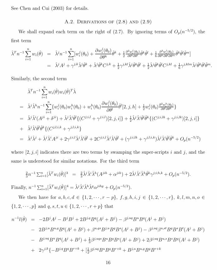
See Chen and Cui (2003) for details.

A.2. Derivations of (2.8) and (2.9)

We shall expand each term on the right of (2.7). By ignoring terms of Op(n−5/2), the

first term

λT n−1n∑

i=1

wi(θ) = λjn−1n∑

i=1

[wji (θ0) +

∂wji (θ0)

∂θkθk + 1

2

∂2wji (θ0)

∂θk∂θl θk θl + 16

∂3wji (θ0)

∂θk∂θl∂θm θkθlθm]

= λjAj + γj,kλj θk + λj θkCj,k + 12γj,klλj θkθl + 1

2λj θk θlCj,kl + 1

6γj,klmλj θkθlθm.

Similarly, the second term

λT n−1n∑

i=1

wi(θ)wi(θ)T λ

= λj λhn−1n∑

i=1

wji (θ0)w

hi (θ0) + wh

i (θ0)∂wj

i (θ0)

∂θlθl[2, j, h] + 1

2wj

i (θ0)∂2wh

i (θ0)

∂θl∂θk

= λj λi(Aji + δji) + λj λiθl(Cj;i,l + γj;i,l)[2, j, i]+ 12λj λiθlθk(Cj;i,lk + γj;i,lk)[2, j, i]

+ λj λiθlθk(Cj,l;i,k + γj,l;i,k

= λj λj + λjλiAji + 2γj;i,lλj λiθl + 2Cj;i,lλj λiθl + (γj;i,lk + γj,l;i,k)λj λiθlθk + Op(n−5/2)

where [2, j, i] indicates there are two terms by swamping the super-scripts i and j, and the

same is understood for similar notations. For the third term

23n−1 ∑n

i=1[λT wi(θ)]

3 = 23λjλiλh(Ajih + αjih) + 2λj λiλhθkγj;i;h,k + Op(n

−5/2).

Finally, n−1 ∑ni=1[λ

T wi(θ)]4 = λj λiλhλgαjihg + Op(n−5/2).

We then have for a, b, c, d ∈ 1, 2, · · · , r − p, f, g, h, i, j ∈ 1, 2, · · · , r, k, l,m, n, o ∈1, 2, · · · , p and q, s, t, u ∈ 1, 2, · · · , r + p that

n−1l(θ) = −2BjAj − BjBj + 2Bj,qBq(Aj + Bj) − βj,uqBuBq(Aj + Bj)

− 2Bj,uBu,qBq(Aj + Bj) + βu,qsBj,uBqBs(Aj + Bj) − βj,uqβu,stBqBsBt(Aj + Bj)

− Bj,uqBuBq(Aj + Bj) + 13βj,uqsBuBqBs(Aj + Bj) + 2βj,uqBu,sBsBq(Aj + Bj)

+ 2γj,k−Bj,qBqBr+k + [12βj,uqBuBqBr+k + Bj,uBu,qBqBr+k

16

− 12βu,qsBj,uBqBsBr+k − βj,uqBu,sBqBsBr+k + 1

2βj,uqβu,stBqBsBtBr+k

+ 12Bj,uqBuBqBr+k − 1

6βj,uqsBuBqBsBr+k − 1

2βj,uqBuBqBr+k,sBs][2, j, r + k]

+ Bj,uBuBr+k,qBq + 14βj,uqβr+k,stBuBqBsBt

+ 2Cj,kBjBr+k −Bj,qBqBr+k[2, j, r + k] + 12βj,uqBuBqBr+k[2, j, r + k]

+ γj,kl−BjBr+kBr+l + Br+kBr+lBj,qBq[3, j, r + k, r + l]

− 12BjBr+kβr+l,uqBuBq[3, j, r + k, r + l] − C j,klBjBr+kBr+l

+ 13γj,klmBjBr+kBr+lBr+m − Bj,uBuBj,qBq − 1

4βj,uqβj,stBuBqBsBt

+ βj,uqBuBqBj,sBs − BjBiAji + BjBi,qBqAji[2, j, i]− 12βj,uqBuBqBiAji[2, j, i]

+ 2γj;i,lBjBiBr+l − BjBiBr+l,qBq + 12βr+l,uqBjBiBuBq − Br+lBiBj,qBq[2, j, i]

+ 12βj,uqBuBqBiBr+l[2, j, i]+ 2BjBiBr+lCj;i,l − (γj;i,lk + γj,l;i,k)BjBiBr+lBr+k

− 23αjihBjBiBh + 2αjihBjBiBh,qBq − αjihβj,uqBuBqBiBh − 2

3AjihBjBiBh

+ 2γj;i;h,kBjBiBhBr+k − 12αjihgBjBiBhBg + Op(n

−5/2).

Applying (A.1) and (A.4), it may be shown that the 3rd to the 18th terms on the right hand

side cancel each other and the application of (A.4) simplifies the 20th term. Keep all the

other terms, we have (2.8).

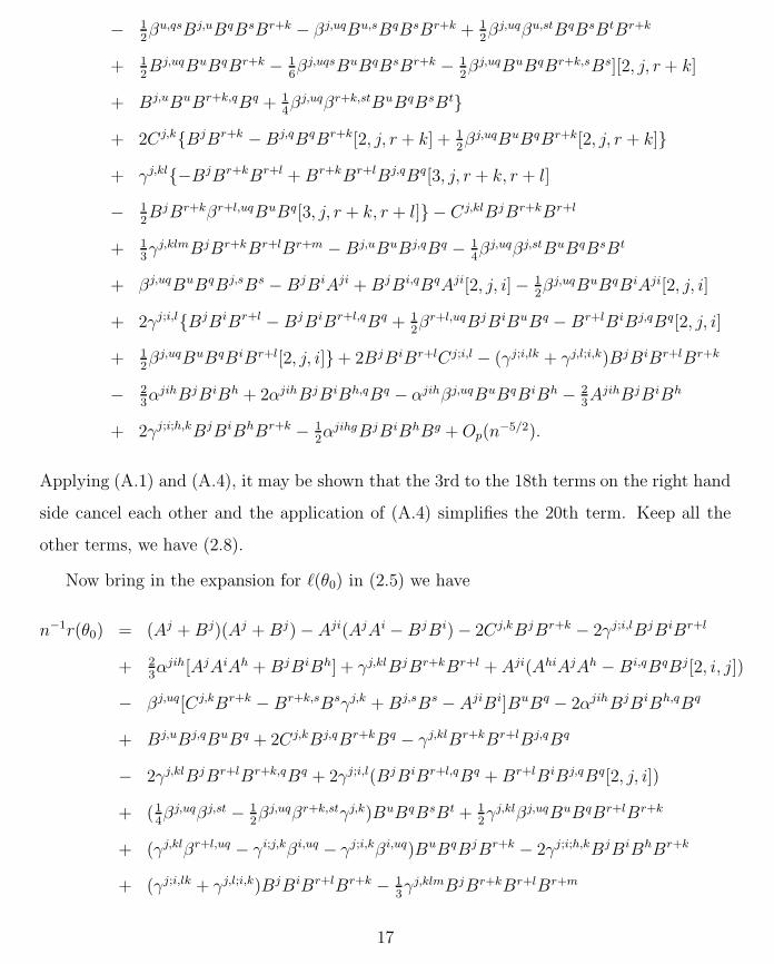
Now bring in the expansion for `(θ0) in (2.5) we have

n−1r(θ0) = (Aj + Bj)(Aj + Bj) − Aji(AjAi − BjBi) − 2Cj,kBjBr+k − 2γj;i,lBjBiBr+l

+ 23αjih[AjAiAh + BjBiBh] + γj,klBjBr+kBr+l + Aji(AhiAjAh − Bi,qBqBj[2, i, j])

− βj,uq[Cj,kBr+k − Br+k,sBsγj,k + Bj,sBs − AjiBi]BuBq − 2αjihBjBiBh,qBq

+ Bj,uBj,qBuBq + 2Cj,kBj,qBr+kBq − γj,klBr+kBr+lBj,qBq

− 2γj,klBjBr+lBr+k,qBq + 2γj;i,l(BjBiBr+l,qBq + Br+lBiBj,qBq[2, j, i])

+ (14βj,uqβj,st − 1

2βj,uqβr+k,stγj,k)BuBqBsBt + 1

2γj,klβj,uqBuBqBr+lBr+k

+ (γj,klβr+l,uq − γi;j,kβi,uq − γj;i,kβi,uq)BuBqBjBr+k − 2γj;i;h,kBjBiBhBr+k

+ (γj;i,lk + γj,l;i,k)BjBiBr+lBr+k − 13γj,klmBjBr+kBr+lBr+m

17

+ 12αjihgBjBiBhBg + (αjihβh,uq − γj;i,lβr+l,uq)BjBiBuBq

+ Cj,klBjBr+kBr+l − 2Cj;i,lBjBiBr+l + 23Ajih(BjBiBh + AjAiAh)

− 2αjihAghAjAiAg + αjgfαihf AjAiAhAg − 12αjihgAjAiAhAg + Op(n

−5/2).(A.7)

As shown in Chen and Cui (2003), the terms appeared on the 3rd line of the above

equation cancel each other. Applying again (A.5), we can express the terms appeared in the

first two lines of (A.7) by

AlAl − AklAkAl − 2Al p+aAp+aAl + 23αklmAkAmAl + 2ωklCp+a,kAp+aAl

+ [2αkl p+a − γp+a,mnωmkωnl]Ap+aAkAl + 2[αl p+a p+b − γp+a;p+b,kωkl]Ap+aAp+bAl

which leads us to (2.9).

A.3. Expansion for R3

We subtract Rl2R

l2 from all the terms appeared in line 4 and below in (2.9). Fortunately

all the terms which do not have Al appeared cancel out with those appeared in Rl2R

l2.

Otherwise, a signed root decomposition of the EL ratio r(θ0) would not be possible. Hence

the remaining terms can be written as 2Rl1R

l3.

By repeatedly employing the formulae (A.5) and (A.6) as well as (A.1), (A.2) and (A.4),

it is shown in Chen and Cui (2003) after some quite involved algebra that Rl3 =

∑6i=1 Rl

3i

where

Rl31 = 3

8AlmAkmAk + 1

3AlkmAkAm − 5

12αlkmAnmAkAn

− 512

αknmAlmAkAn + 49αlknαomnAmAkAo − 1

4αlknmAmAkAn,

Rl32 = Alk p+aAp+aAk + Al p+a p+bAp+aAp+b − 1

2ωknωmlCp+a,kmAp+aAn

− ωklCp+a;p+b,kAp+aAp+b + 12ωkmCp+a,kAlmAp+a + 1

2AlkAk p+aAp+a

+ Alp+aAp+a p+bAp+b + 12Alp+aAp+akAk − 1

2ωkmωnlCp+a,nCp+a,kAm

− ωklωmnCn,kCp+a,mAp+a − ωklCp+a,kAp+a p+bAp+b,

Rl33 = 1

2[γm,voωvnωolωkm − 2

3αnmlωkm]Cp+a,kAp+aAn + 1

2γp+b,koωknωolωmvCp+b,mAnAv

18

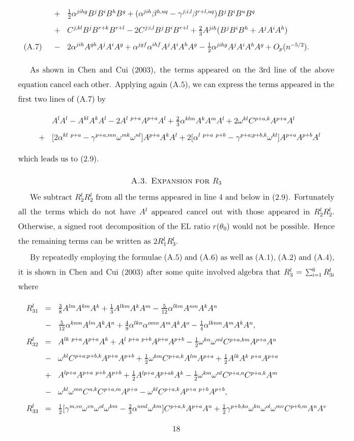
+ [12γp+b,koωknωol − αlnp+b]Ap+b p+aAp+aAn + ωvk[ωnl(γk;p+a,n + γp+a;k,n)

− αlkp+b − 12γp+b,mnωmlωnk]Cp+a,vAp+aAp+b + γp+a,koωonωmlωkvCv,mAp+aAn

+ [12γp+b,mkωmlωkn − αlnp+b]An p+aAp+aAp+b,

Rl34 = γp+a;p+b,nωnoωmlCo,mAp+aAp+b − αp+a p+b p+cAl p+cAp+aAp+b

+ [(γp+c;p+a,n + γp+a;p+c,n)ωnl − 2αl p+a p+c]Ap+c p+bAp+aAp+b

+ (γp+c;p+a,o + γp+a;p+c,o)ωonωklCp+c,kAp+aAn − αlk p+aAm p+aAkAm

+ αp+a p+b p+cωmlCp+c,mAp+aAp+b − 23αlkmAm p+aAp+aAk

− [32αko p+a + 1

4γp+a,mnωmkωno]AloAp+aAk − 2αk p+a p+bAlp+bAp+aAk

− [αm p+a p+b + γp+a;p+b,kωkm]AlmAp+aAp+b,

Rl35 = [1

2αlk p+aαmn p+a − 1

8ωl′lωm′mωn′nωk′kγp+a,l′m′

γp+a,n′k′

]AmAnAk

+ [2αp+a kfαlmf − αlkm p+a − 13αlmn(αkn p+a − 1

2γp+a,m′n′

ωm′kωn′n)

− 12ωm′mωk′kωl′l(ωl′vγp+a,m′l′γv,l′k′ − 1

3γp+a,m′k′l′)]Ap+aAkAm

− 12[3αlk p+a p+b + 2

3αklv(αv p+a p+b − 1

2γp+a;p+b,nωnv)

+ (αkvp+a − 12γp+a,mnωmkωnv)(αlvp+b − 1

2γp+b,m′n′

ωm′lωn′v)]Ap+aAp+bAk

+ [αl p+a fαp+b p+c f − αl p+a p+b p+c − (αlk p+c − 12γp+c,mnωmlωnk)

× (αk p+a p+b − γp+a;p+b,v)ωvk]Ap+aAp+bAp+c and

Rl36 = 2αl p+a fαmp+bf + αlmf αp+a p+b f + ωm′mωn′l[1

2ωokωvkγp+a,om′

γp+b,vn′

− 12(γp+c;p+a,m′

+ γp+a;p+c,m′

)(γp+c;p+b,n′

+ γp+b;p+c,n′

)

− ωkoγp+b,n′k(γo,m′;p+a + γo;p+a,m′

) − 12αp+a p+b p+cγp+c,m′n′

− 12ωkoγo,m′n′

γp+a;p+b,k + 12γp+a;p+b,m′n′

+ 12γp+a,n;p+b,m′

]Ap+aAp+bAm.

A.4. Proof of Theorems 1 and 2.

The proof of Theorem 1 is divided into two parts. In the first part, we derive the

cumulants of√

nR. In the second part, we establish an Edgeworth expansion for the signed

19

root which then leads to an Edgeworth expansion for the EL ratio r(θ0).

Cumulants of the signed root R. Since the cumulants of order higher than four are of

O(n−2) or smaller, we only need to derive the first four cumulants. As the first and the third

cumulants are easier to derive than the second and the fourth, we present them first. From

(2.10) and (2.11), and the fact that Rj3 is the product of four zero-mean averages, we have

E(Rl1) = 0, E(Rl

2) = n−1µl and E(Rj3) = O(n−2)

where µl = −16n−1αlkk. Therefore, the first order cumulant is

cum(Rl) = n−1µl + O(n−2).(A.8)

The joint third-order cumulants

cum(Rl, Ro, Rv) = E(RlRoRv) −E(Rl)E(RoRv)[3] + 2E(Rl)E(Ro)E(Rv)[3]

= E(Rl1R

o1R

v1) + E(Rl

2Ro1R

v1)[3]− E(Rl

2)E(Ro1R

v1)[3] + O(n−3).

We note that

E(Rl1R

o1) = n−1δlo and

E(Rl2R

o1) = n−2[−1

2(αlokk − δlo) − αlo p+a p+a + 1

3αlkmαokm + ωklγp+a;o;p+a,k

+ (αlk p+a − 12ωmkωnlγp+a,mn)αok p+a + (αl p+a p+b − ωklγp+a;p+b,k)αo p+a p+b].

Write Rl2 = Rl

21 + Rl22 where Rl

21 = −12AklAk + 1

3αklmAkAm and Rl

22 contains the rest of

the terms appeared in (2.11). We have

E(Rl21) = −1

6n−1αlkk,

E(Rl22R

o1R

v1) = E(Rl

22)δov + O(n−3) = O(n−3) and

E(Rl21R

o1R

v1) = n−2(−1

6αlkkδov − 1

3αlov) + O(n−3).

Thus,

E(Rl2R

o1R

v1) = E(Rl

2)E(Ro1R

v1) − 1

3E(Rl

1Ro1R

v1) + O(n−3),(A.9)

20

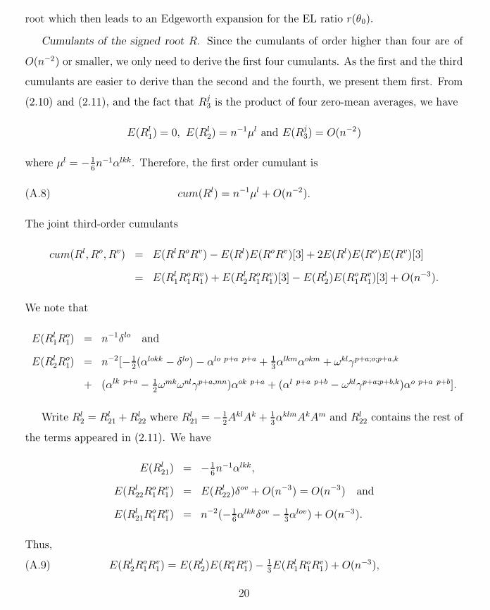
which means that

cum(Rl, Ro, Rv) = O(n−3).(A.10)

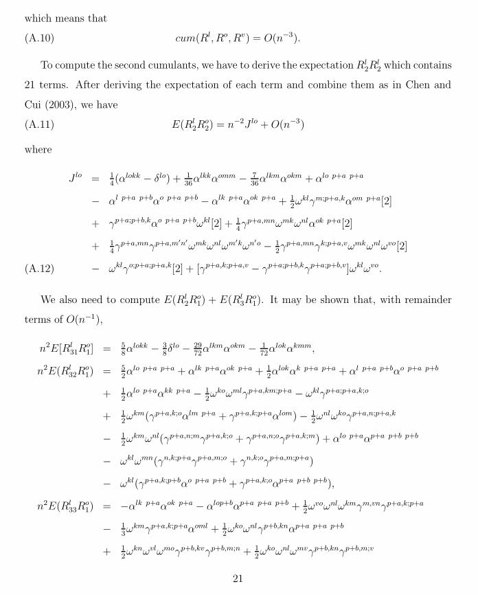
To compute the second cumulants, we have to derive the expectation Rl2R

l2 which contains

21 terms. After deriving the expectation of each term and combine them as in Chen and

Cui (2003), we have

E(Rl2R

o2) = n−2J lo + O(n−3)(A.11)

where

J lo = 14(αlokk − δlo) + 1

36αlkkαomm − 7

36αlkmαokm + αlo p+a p+a

− αl p+a p+bαo p+a p+b − αlk p+aαok p+a + 12ωklγm;p+a,kαom p+a[2]

+ γp+a;p+b,kαo p+a p+bωkl[2] + 14γp+a,mnωmkωnlαok p+a[2]

+ 14γp+a,mnγp+a,m′n′

ωmkωnlωm′kωn′o − 12γp+a,mnγk;p+a,vωmkωnlωvo[2]

− ωklγo;p+a;p+a,k[2] + [γp+a,k;p+a,v − γp+a;p+b,kγp+a;p+b,v]ωklωvo.(A.12)

We also need to compute E(Rl2R

o1) + E(Rl

3Ro1). It may be shown that, with remainder

terms of O(n−1),

n2E[Rl31R

o1] = 5

8αlokk − 3

8δlo − 29

72αlkmαokm − 1

72αlokαkmm,

n2E(Rl32R

o1) = 5

2αlo p+a p+a + αlk p+aαok p+a + 1

2αlokαk p+a p+a + αl p+a p+bαo p+a p+b

+ 12αlo p+aαkk p+a − 1

2ωkoωmlγp+a,km;p+a − ωklγp+a;p+a,k;o

+ 12ωkm(γp+a,k;oαlm p+a + γp+a,k;p+aαlom) − 1

2ωnlωkoγp+a,n;p+a,k

− 12ωkmωnl(γp+a,n;mγp+a,k;o + γp+a,n;oγp+a,k;m) + αlo p+aαp+a p+b p+b

− ωklωmn(γn,k;p+aγp+a,m;o + γn,k;oγp+a,m;p+a)

− ωkl(γp+a,k;p+bαo p+a p+b + γp+a,k;oαp+a p+b p+b),

n2E(Rl33R

o1) = −αlk p+aαok p+a − αlop+bαp+a p+a p+b + 1

2ωvoωnlωkmγm,vnγp+a,k;p+a

− 13ωkmγp+a,k;p+aαoml + 1

2ωkoωnlγp+b,knαp+a p+a p+b

+ 12ωknωvlωmoγp+b,kvγp+b,m;n + 1

2ωkoωnlωmvγp+b,knγp+b,m;v

21

− ωvkαlk p+aγp+a,v;o + ωvkωnl(γk;p+a,n + γp+a;k,n)γp+a,v;o

+ 12ωmlωknγp+a,mkαon p+a + ωnoωmlωkvγp+a,knγv,m;p+a,

n2E(Rl34R

o1) = −4αl p+a p+bαo p+a p+b − 5

3αlomαm p+a p+a − 7

2αlk p+aαok p+a

− αlo p+aαkk p+a − αlo p+aαp+a p+b p+b + ωmlωnkγk,m;oγp+a;p+a,n

+ ωnl(γp+b;p+a,n + γp+a;p+b,n)αo p+a p+b

+ ωnoωkl(γp+b;p+a,n + γp+a;p+b,n)γp+b,k;p+a + ωmlγp+b,m;oαp+a p+a p+b

− 14ωmoωnkγp+a,mnαlk p+a − ωkmγp+a;p+a,kαlom,

n2E(Rl35R

o1) = 1

2αlo p+aαkk p+a + αlk p+aαok p+a − 3

2αlo p+a p+a − 1

3αlokαk p+a p+a

+ 16ωnvαlovγp+a;p+a,n − 1

2αlk p+aαok p+a + 1

4ωmoωnvαlvp+aγp+a,mn[2]

− 18ωl′lωm′oωn′kωk′kγp+a,l′m′

γp+a,n′k′

− 38ωmoωnvωm′lωn′vγp+a,mnγp+a,m′n′

,

n2E(Rl36R

o1) = 2αlk p+aαok p+a + 2αl p+a p+bαo p+a p+b + αlokαk p+a p+b

+ αlo p+aαp+a p+b p+b + 12ωm′oωn′lωmkωvkγp+a,mm′

γp+a,vn′

− 12ωm′oωn′l(γp+b;p+a,m′

+ γp+a;p+b,m′

)(γp+b;p+a,n′

+ γp+a;p+b,n′

)

− ωm′oωn′lωkm(γm,m′ ;p+a + γm;p+a,m′

)γp+a,n′k

− 12ωm′oωn′lαp+a p+a p+bγp+b,m′n′ − 1

2ωm′oωn′lωkmγm,m′n′

γp+a;p+a,k

+ 12ωm′oωn′l(γp+a;p+a,m′n′

+ γp+a,n;p+a,m′

),

n2E(Rl2R

o1) = −1

2(αlokk − δlo) − αlo p+a p+a + 1

3αlkmαokm + αl p+a p+bαo p+a p+b

+ αlk p+aαok p+a + ωklγp+a;o;p+a,k − 12ωmkωnlγp+a,mnαok p+a

− ωklγp+a;p+b,kαo p+a p+b.

In summary,

E(Rl2R

o1) + E(Rl

3Ro1) = n−2K lo + O(n−3)(A.13)

where

K lo = 18(αlokk + δlo) − 5

72αlkmαokm − 1

72αlokαkmm − 1

2αlokαk p+a p+a

22

− 12ωkmγp+a,k;oαlm p+a − 2

3ωkmγp+a,k;p+aαlom + 1

4ωmlωnkαok p+aγp+a,mn

+ 12ωnlωkm(γp+a,k;oγp+a,n;m − γp+a,n;oγp+a,k;m)

+ 12ωknωvlωmo(γp+a,mvγp+a,k;n − γp+a,kvγp+a,m;n)

+ ωmoωvlωkn(γp+a,kmγp+a;n,v − γp+a,kvγp+a;n,m)

+ 18ωm′lωmoωn′kωnk(γp+a,mnγp+a,m′n′ − γp+a,mm′

γp+a,nn′

).

In light of (A.11) and (A.13), we have

cum(Rl, Ro) = n−1δlo + n−2∆lo + O(n−3)(A.14)

where

∆lo = K lo[2] + J lo − µlµo.(A.15)

The joint fourth-order cumulants of R is

cum(Rl, Rk, Rm, Rn) = E(RlRkRmRn) −E(RlRk)E(RmRn)[3]

− E(Rl)E(RkRmRn)[4] + 2E(Rl)E(Rk)E(RmRn)[6]

− 6E(Rl)E(Rk)E(Rm)E(Rn)

= E(Rl1R

k1R

m1 Rn

1 ) + E(Rl2R

k1R

m1 Rn

1 )[4] + E(Rl3R

k1R

m1 Rn

1 )[4](A.16)

+ E(Rl2R

k2R

m1 Rn

1 )[6]− E(Rl1R

k1]E(Rm

1 Rn1 )[3]

− E(Rl2R

k1)E(Rm

1 Rn1 )[12] −E(Rl

3Rk1)E(Rm

1 Rn1 )[12]

− E(Rl2R

k2)E(Rm

1 Rn1 )[6]− E(Rl

2)E(Rk1R

m1 Rn

1 )[4]

− E(Rl2)E(Rk

2Rm1 Rn

1 )[12] + 2E(Rl2)E(Rk

2)E(Rm1 Rn

1 )[6] + O(n−4).

From (A.9), we immediately have

E(Rl2)E(Rk

1Rm1 Rn

1 )[4] + E(Rk2R

m1 Rn

1 )[12] − 2E(Rk2)E(Rm

1 Rn1 )[6] = O(n−4)

which means the sum of the last three terms in (A.16) is negligible.

23

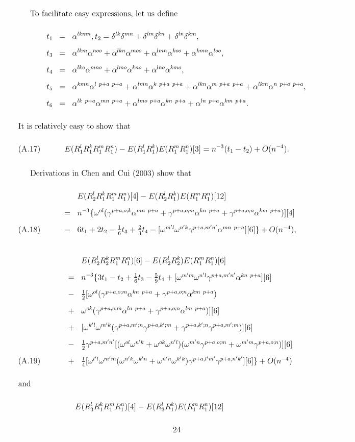
To facilitate easy expressions, let us define

t1 = αlkmn, t2 = δlkδmn + δlmδkn + δlnδkm,

t3 = αlkmαnoo + αlknαmoo + αlmnαkoo + αkmnαloo,

t4 = αlkoαmno + αlmoαkno + αlnoαkmo,

t5 = αkmnαl p+a p+a + αlmnαk p+a p+a + αlknαm p+a p+a + αlkmαn p+a p+a,

t6 = αlk p+aαmn p+a + αlmo p+aαkn p+a + αln p+aαkm p+a.

It is relatively easy to show that

E(Rl1R

k1R

m1 Rn

1 ) − E(Rl1R

k1)E(Rm

1 Rn1 )[3] = n−3(t1 − t2) + O(n−4).(A.17)

Derivations in Chen and Cui (2003) show that

E(Rl2R

k1R

m1 Rn

1 )[4]− E(Rl2R

k1)E(Rm

1 Rn1 )[12]

= n−3ωol(γp+a,o;kαmn p+a + γp+a,o;mαkn p+a + γp+a,o;nαkm p+a)][4]

− 6t1 + 2t2 − 16t3 + 2

3t4 − [ωm′lωn′kγp+a,m′n′

αmn p+a][6]+ O(n−4),(A.18)

E(Rl2R

k2R

m1 Rn

1 )[6] −E(Rl2R

k2)E(Rm

1 Rn1 )[6]

= n−33t1 − t2 + 16t3 − 5

9t4 + [ωm′mωn′lγp+a,m′n′

αkn p+a][6]

− 12[ωol(γp+a,o;mαkn p+a + γp+a,o;nαkm p+a)

+ ωok(γp+a,o;mαln p+a + γp+a,o;nαlm p+a)][6]

+ [ωk′lωm′k(γp+a,m′;nγp+a,k′;m + γp+a,k′ ;nγp+a,m′;m)][6]

− 12γp+a,m′n′

[(ωolωn′k + ωokωn′l)(ωm′nγp+a,o;m + ωm′mγp+a,o;n)][6]

+ 14[ωl′lωm′m(ωn′kωk′n + ωn′nωk′k)γp+a,l′m′

γp+a,n′k′

][6]+ O(n−4)(A.19)

and

E(Rl3R

k1R

m1 Rn

1 )[4] − E(Rl3R

k1)E(Rm

1 Rn1 )[12]

24

= n−32t1 − 19t4 + [ωn′lωk′k(γp+a,k′;nγp+a,n′ ;m + γp+a,n′;nγp+a,k′ ;m)][6]

+ 12[γp+a,m′n′

(ωolωn′k + ωokωn′l)(ωm′nγp+a,o;m + ωm′mγp+a,o;n)][6]

− 14[ωl′lωm′m(ωn′kωk′n + ωn′nωk′k)γp+a,l′m′

γp+a,n′k′

][6]+ O(n−4).(A.20)

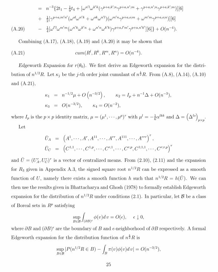
Combining (A.17), (A.18), (A.19) and (A.20) it may be shown that

cum(Rl, Rk, Rm, Rn) = O(n−4).(A.21)

Edgeworth Expansion for r(θ0). We first derive an Edgeworth expansion for the distri-

bution of n1/2R. Let κj be the j-th order joint cumulant of n1

2 R. From (A.8), (A.14), (A.10)

and (A.21),

κ1 = n−1/2µ + O(n−3/2

), κ2 = Ip + n−1∆ + O(n−3),

κ3 = O(n−3/2), κ4 = O(n−2),

where Ip is the p× p identity matrix, µ = (µ1, · · · , µp)τ with µl = −16αlkk and ∆ =

(∆lo

)

p×p.

Let

UA =(A1, · · · , Ar, A11, · · · , Arr, A111, · · · , Arrr

)τ,

UC =(C1,1, · · · , C1,p, · · · , Cr,1, · · · , Cr,p, C1;1,1, · · · , Cr;r,p

)τ

and U = (U τA, U τ

C)τ is a vector of centralized means. From (2.10), (2.11) and the expansion

for R3 given in Appendix A.3, the signed square root n1/2R can be expressed as a smooth

function of U , namely there exists a smooth function h such that n1/2R = h(U ). We can

then use the results given in Bhattacharya and Ghosh (1978) to formally establish Edgeworth

expansion for the distribution of n1/2R under conditions (2.1). In particular, let B be a class

of Boreal sets in Rp satisfying

supB∈B

∫

(∂B)εφ(v)d v = O(ε), ε ↓ 0,

where ∂B and (∂B)ε are the boundary of B and ε-neighborhood of ∂B respectively. A formal

Edgeworth expansion for the distribution function of n1

2 R is

supB∈B

|P (n1/2R ∈ B) −∫

Bπ(v)φ(v)d v| = O(n−3/2),

25

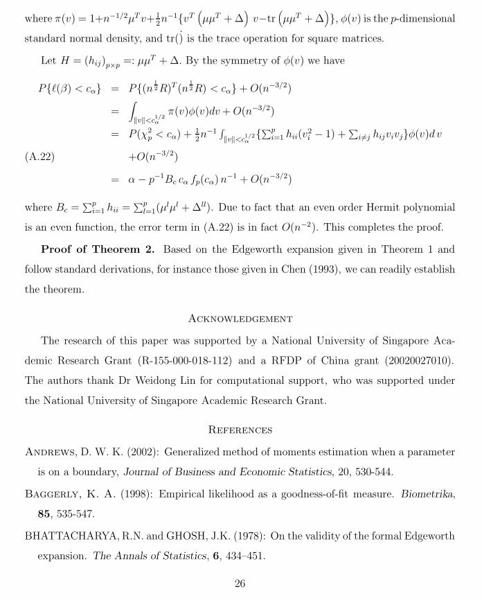
where π(v) = 1+n−1/2µT v+12n−1vT

(µµT + ∆

)v−tr

(µµT + ∆

), φ(v) is the p-dimensional

standard normal density, and tr() is the trace operation for square matrices.

Let H = (hij)p×p =: µµT + ∆. By the symmetry of φ(v) we have

P`(β) < cα = P(n 1

2 R)T (n1

2 R) < cα + O(n−3/2)

=∫

‖v‖<c1/2

α

π(v)φ(v)dv + O(n−3/2)

= P (χ2p < cα) + 1

2n−1

∫‖v‖<c

1/2

α∑p

i=1 hii(v2i − 1) +

∑i6=j hijvivjφ(v)d v

+O(n−3/2)(A.22)

= α − p−1Bc cα fp(cα)n−1 + O(n−3/2)

where Bc =∑p

i=1 hii =∑p

l=1(µlµl + ∆ll). Due to fact that an even order Hermit polynomial

is an even function, the error term in (A.22) is in fact O(n−2). This completes the proof.

Proof of Theorem 2. Based on the Edgeworth expansion given in Theorem 1 and

follow standard derivations, for instance those given in Chen (1993), we can readily establish

the theorem.

Acknowledgement

The research of this paper was supported by a National University of Singapore Aca-

demic Research Grant (R-155-000-018-112) and a RFDP of China grant (20020027010).

The authors thank Dr Weidong Lin for computational support, who was supported under

the National University of Singapore Academic Research Grant.

References

Andrews, D. W. K. (2002): Generalized method of moments estimation when a parameter

is on a boundary, Journal of Business and Economic Statistics, 20, 530-544.

Baggerly, K. A. (1998): Empirical likelihood as a goodness-of-fit measure. Biometrika,

85, 535-547.

BHATTACHARYA, R.N. and GHOSH, J.K. (1978): On the validity of the formal Edgeworth

expansion. The Annals of Statistics, 6, 434–451.

26

BHATTACHARYA, R.N. and RAO, R.R. (1976): Normal Approximation and Asymptotic

Expansions. Wiley, New York.

Brown, B. W. and Newey, W. K. (2002): “Generalized method of moments, efficient

bootstrapping, and improved inference”, Journal of Business and Economic Statistics, 20,

507-517.

CHEN S. X. (1993): On the coverage accuracy of empirical likelihood regions for linear

regression model, The Annals of the Institute of Statistical Mathematics, 45, 621-637.

CHEN, S. X. (1994). Empirical likelihood confidence intervals for linear regression coeffi-

cients. Journal Multivariate Analysis. 49, 24-40.

CHEN, S. X. AND CUI, H. J. (2003): On the Bartlett properties of empirical likelihood with

moment restrictions, Technical Report, Department of Statistics, Iowa State University.

DICICCIO, T. J., HALL, P. AND ROMANO, J. P. (1991): Empirical likelihood is Bartlett

correctable. The Annals of Statistics, 19, 1053-1061.

Donald, S. G., Imbens, G. W. AND Newey, W. K. (2003): Empirical likelihood

estimation and consistent tests with conditional moment restrictions. Journal of Econo-

metrics, 117, 55-93.

Hansen, B. E. and WEST, K. D. (2002): Generalized method of moments and macroe-

conomics, Journal of Business and Economic Statistics, 20, 460-469.

Hansen, L. P. (1982): Large sample properties of generalized method of moments estima-

tors, Econometrica, 50, 1029-1054.

HALL, P. (1992): The bootstrap and Edgeworth Expansions Springer-Verlag.

HALL, P. AND LA SCALA, B. (1990): Methodology and algorithms of empirical likelihood.

International Statistical Reviews 58, 109–127.

Imbens, G. W. (1997): One-step estimators for over-identified generalized method of mo-

ments models, Review of Economic Studies, 64, 359-383.

Imbens, G. W. (2002): Generalized method of moments and empirical likelihood equations,

27

Journal of Business and Economic Statistics, 20, 493-506.

Jagannathan, R. (2002): “Generalized method of moments: Applications in finance”,

Journal of Business and Economic Statistics, 20, 470-481.

JING, B. Y. and WOOD, A. T. A. (1996). Exponential empirical likelihood is not Bartlett

correctable. Ann. Statist. 24 365-369.

KITAMURA, Y. (1997): Empirical likelihood methods with weakly dependent processes.

The Annals of Statistics, 25, 2084-2102.

KITAMURA, Y. (2001): Asymptotic optimality of empirical likelihood for testing moment

restrictions. Econometrica, 69, 1661-1672.

KITAMURA, Y. AND STUTZER, M. (1997): An information-theoretic alternative to gen-

eralized method of moments estimation. Econometrica, 65, 861-874.

KITAMURA, Y., Tripathi, G. and Ahn, H. (2002): Empirical likelihood-based inference

in conditional moment restriction models. Manuscript.

Newey, W. K. and Smith, R. J. (2004): Higher order properties of GMM and generalized

empirical likelihood estimators. Econometrica to appear.

OWEN, A. B. (1988): Empirical likelihood ratio confidence intervals for a single functional.

Biometrika 75, 237–249.

OWEN, A. B. (2001). Empirical Likelihood. Chapman and Hall.

QIN, J. AND LAWLESS, J. (1994): Empirical likelihood and general estimation equa-

tions, The Annals of Statistics, 22, 300-325.

Smith, R. J. (1997): Alternative Semi-parametric likelihood approaches to generalized

method of moments estimation, Economic Journal, 107, 503-519.

SKOVGAARD, IB. M. (1981): Transformation of an Edgeworth expansion by a sequence

of smooth functions. Scand. J. Statist. 8, 207-217.

Tripathi, G. AND KITAMURA, Y. (2002): Testing conditional moment restrictions.

Manuscript.

28

Table 1. Empirical coverage (in percentage) and averaged length of the EL confidence interval

Iα, the Bartlett corrected (BC) EL interval Iα,bc and the dircet Bootstrap (BT) calibrated

confidence interval Iα,bt for the normal mean example.

(a) N(0, 1)

Nominal level 90% 95%

Sample Size EL BC BT EL BCBT

20 coverage 84.66 89.40 86.88 91.12 93.04 93.34

length 0.636 0.817 0.791 0.757 0.967 0.967

30 coverage 86.30 89.60 87.80 92.60 93.80 93.10

length 0.552 0.662 0.640 0.659 0.789 0.781

40 coverage 86.47 89.48 87.98 93.49 95.09 94.79

length 0.492 0.558 0.548 0.588 0.668 0.665

60 coverage 86.70 89.00 87.90 93.50 94.50 92.90

length 0.448 0.492 0.437 0.536 0.588 0.527

(b) N(1, 2)

Nominal level 90% 95%

Sample Size EL BC BT EL BC BT

20 coverage 80.02 87.99 85.57 86.78 91.62 90.41

length 0.656 0.898 0.854 0.781 1.061 1.084

30 coverage 82.85 89.47 88.16 88.87 93.68 93.88

length 0.6547 0.7740 0.752 0.739 0.883 0.879

40 coverage 85.77 89.94 88.92 91.77 93.70 93.70

length 0.496 0.590 0.572 0.592 0.703 0.701

60 coverage 87.47 90.28 89.68 92.69 94.19 94.29

length 0.411 0.454 0.446 0.492 0.543 0.540

29

Table 2. Empirical coverage (in percentage) and averaged length of the EL confidence interval

Iα and the Bartlett corrected (BC) EL interval Iα,bc for the panel data model (4.1)

(a) θ = 0.5

Nominal level 90% 95%

Sample Size EL BC BT EL BC BT

50 coverage 81.7 87.3 87.7 88.8 93.6 93.9

length 0.603 0.723 0.733 0.736 0.876 0.880

100 coverage 87.4 89.9 89.9 94.3 95.7 95.5

length 0.425 0.461 0.462 0.511 0.556 0.560

(b) θ = 0.9

Nominal level 90% 95%

Sample Size EL BC BT EL BC BT

50 coverage 84.4 89.6 89.2 90.2 94.9 95.1

length 0.545 0.648 0.656 0.667 0.787 0.800

100 coverage 87.3 89.1 89.2 92.6 94.4 94.3

length 0.373 0.401 0.402 0.4494 0.4847 0.487

30