Research Article Empirical Likelihood for Partial...
11
Research Article Empirical Likelihood for Partial Parameters in ARMA Models with Infinite Variance Jinyu Li, 1 Wei Liang, 2 and Shuyuan He 3 1 School of Sciences, China University of Mining and Technology, Xuzhou 221116, China 2 School of Mathematical Sciences, Xiamen University, Xiamen 361005, China 3 School of Mathematical Sciences, Capital Normal University, Beijing 100048, China Correspondence should be addressed to Jinyu Li; [email protected] Received 31 March 2014; Accepted 24 August 2014; Published 2 September 2014 Academic Editor: Charalampos Tsitouras Copyright © 2014 Jinyu Li et al. is is an open access article distributed under the Creative Commons Attribution License, which permits unrestricted use, distribution, and reproduction in any medium, provided the original work is properly cited. is paper proposes a profile empirical likelihood for the partial parameters in ARMA(, ) models with infinite variance. We introduce a smoothed empirical log-likelihood ratio statistic. Also, the paper proves a nonparametric version of Wilks’s theorem. Furthermore, we conduct a simulation to illustrate the performance of the proposed method. 1. Introduction Consider the stationary ARMA(, ) time series { } gener- ated by = 1 −1 +⋅⋅⋅+ − + + 1 −1 +⋅⋅⋅+ − , (1) where the innovation process { } is a sequence of i.i.d. random variables. When ( 2 )=∞, model (1) is an infinite variance autoregressive moving average (IVARMA) model, which defines a heavy-tailed process { }. For model (1), statistical inference has been explored in many studies (see, e.g., [1, 2]). Recently, for example, Pan et al. [3] and Zhu and Ling [4] proposed a weighted least absolute deviations esti- mator (WLADE) for model (1) and obtained the asymptotic normality. However, in the building of ARMA models, we are usually only interested in statistical inference for partial parameters. For example, in the sparse coefficient (a part of zero coef- ficients) ARMA models, it is necessary to determine which coefficient is zero. For model (1), one traditional method is to construct confidence regions for the partial parameters of interest by normal approximation as in [3]. However, since the limit distribution depends on the unknown nuisance parameters and density function of the errors, estimating the asymptotic variance is not a trivial task. Based on these, this paper tries to put forward a new method for the esti- mation of partial parameters of ARMA models. We propose an empirical likelihood method, which was introduced by Owen [5, 6]. Based on the estimating equations of WLADE, a smoothed profile empirical likelihood ratio statistic is derived, and a nonparametric version of Wilks’s theorem is proved. erefore, we can construct confidence regions for the partial parameters of interest. Also, simulations suggest that, for relative small sample cases, the empirical likelihood confidence regions are more accurate than those confidence regions constructed by the normal approximation based on the WLADE proposed by Pan et al. [3]. As an effective nonparametric inference method, the empirical likelihood method produces confidence regions whose shape and orientation are determined entirely by the data and therefore avoids secondary estimation. In the past two decades, the empirical likelihood method has been extended to many applications [7]. ere are also many studies of empirical likelihood method for autoregressive models. Monti [8] considered the empirical likelihood in the frequency domain; Chuang and Chan [9] developed the empirical likelihood for unstable autoregressive models with innovations being a martingale difference sequence with finite variance; Chan et al. [10] applied the empirical Hindawi Publishing Corporation Journal of Applied Mathematics Volume 2014, Article ID 868970, 10 pages http://dx.doi.org/10.1155/2014/868970
Transcript of Research Article Empirical Likelihood for Partial...
Research ArticleEmpirical Likelihood for Partial Parameters in ARMA Modelswith Infinite Variance
Jinyu Li1 Wei Liang2 and Shuyuan He3
1 School of Sciences China University of Mining and Technology Xuzhou 221116 China2 School of Mathematical Sciences Xiamen University Xiamen 361005 China3 School of Mathematical Sciences Capital Normal University Beijing 100048 China
Correspondence should be addressed to Jinyu Li ljycumt163com
Received 31 March 2014 Accepted 24 August 2014 Published 2 September 2014
Academic Editor Charalampos Tsitouras
Copyright copy 2014 Jinyu Li et al This is an open access article distributed under the Creative Commons Attribution License whichpermits unrestricted use distribution and reproduction in any medium provided the original work is properly cited
This paper proposes a profile empirical likelihood for the partial parameters in ARMA(119901 119902) models with infinite variance Weintroduce a smoothed empirical log-likelihood ratio statistic Also the paper proves a nonparametric version of Wilksrsquos theoremFurthermore we conduct a simulation to illustrate the performance of the proposed method
1 Introduction
Consider the stationary ARMA(119901 119902) time series 119910119905 gener-
ated by
119910119905= 1205931119910119905minus1
+ sdot sdot sdot + 120593119901119910119905minus119901
+ 120576119905+ 1205991120576119905minus1
+ sdot sdot sdot + 120599119902120576119905minus119902
(1)
where the innovation process 120576119905 is a sequence of iid
random variables When 119864(1205762119905) = infin model (1) is an infinite
variance autoregressive moving average (IVARMA) modelwhich defines a heavy-tailed process 119910
119905 For model (1)
statistical inference has been explored in many studies (seeeg [1 2]) Recently for example Pan et al [3] and Zhu andLing [4] proposed a weighted least absolute deviations esti-mator (WLADE) for model (1) and obtained the asymptoticnormality
However in the building ofARMAmodels we are usuallyonly interested in statistical inference for partial parametersFor example in the sparse coefficient (a part of zero coef-ficients) ARMA models it is necessary to determine whichcoefficient is zero For model (1) one traditional method isto construct confidence regions for the partial parameters ofinterest by normal approximation as in [3] However sincethe limit distribution depends on the unknown nuisanceparameters and density function of the errors estimating
the asymptotic variance is not a trivial task Based on thesethis paper tries to put forward a new method for the esti-mation of partial parameters of ARMA models We proposean empirical likelihood method which was introduced byOwen [5 6] Based on the estimating equations of WLADEa smoothed profile empirical likelihood ratio statistic isderived and a nonparametric version of Wilksrsquos theorem isproved Therefore we can construct confidence regions forthe partial parameters of interest Also simulations suggestthat for relative small sample cases the empirical likelihoodconfidence regions are more accurate than those confidenceregions constructed by the normal approximation based onthe WLADE proposed by Pan et al [3]
As an effective nonparametric inference method theempirical likelihood method produces confidence regionswhose shape and orientation are determined entirely bythe data and therefore avoids secondary estimation In thepast two decades the empirical likelihood method has beenextended to many applications [7] There are also manystudies of empirical likelihood method for autoregressivemodels Monti [8] considered the empirical likelihood inthe frequency domain Chuang and Chan [9] developedthe empirical likelihood for unstable autoregressive modelswith innovations being a martingale difference sequencewith finite variance Chan et al [10] applied the empirical
Hindawi Publishing CorporationJournal of Applied MathematicsVolume 2014 Article ID 868970 10 pageshttpdxdoiorg1011552014868970
2 Journal of Applied Mathematics
likelihood to near unit root AR(1) model with infinite vari-ance errors Li et al [11 12] respectively used the empiricallikelihood to infinite variance AR(119901) models and model (1)
The rest of the paper is organized as follows In Section 2we propose the profile empirical likelihood for the parametersof interest and show the main result Section 3 provides theproofs of the main results Some simulations are conductedin Section 4 to illustrate our approach Conclusions are givenin Section 5
2 Methodology and Main Results
First the parameter space is denoted by Θ sub 119877119901+119902 whichcontains the true value 120579
0of the parameter 120579 as an inner point
For 120579 = (1205931 120593
119901 1205991 120599
119902) put
120576119905(120579) =
119910119905minus
119901
sum119894=1
120593119894119910119905minus119894
minus
119902
sum119895=1
120599119895120576119905minus119895
(120579) if 119905 gt 0
0 if 119905 le 0
(2)
where 119910119905equiv 0 for all 119905 le 0 and note that 120576
119905(1205790) = 120576119905 because
of this truncationWe define the objective function as
119878119899(120579) =
119899
sum119905=119906+1
119908119905
1003816100381610038161003816120576119905 (120579)1003816100381610038161003816 (3)
where 119906 ge max(119901 119902) and the weight function 119908119905= 1(1+
sum119905minus1
119896=1119896minus120572|119910119905minus119896|)4 depending on a constant 120572 gt 2 The
WLADE denoted by 120579 is a lacol minimizer of 119878119899(120579) in
a neighborhood of 1205790[3] Denote 119860
119905(120579) = (119860
1199051(120579)
119860119905119901+119902
(120579))120591 where119860
119905119894(120579) = minus120597120576
119905(120579)120597120579
119894 By (8119) of Brock-
well and Davis [13] it holds for 119905 gt max(119901 119902) that
119860119905119894(120579) +
119902
sum119895=1
120599119895119860119905minus119895119894
(120579) = 119910119905minus119894 119894 = 1 119901
119860119905119894+119901
(120579) +
119902
sum119895=1
120599119895119860119905minus119895119894+119901
(120579) = 120576119905minus119894(120579) 119894 = 1 119902
(4)
Hence 120579 satisfies estimating equation
1
119899 minus 119906
119899
sum119905=119906+1
119908119905119860119905(120579) sgn 120576
119905(120579) = 0 (5)
where sgn(119909) = minus1 for 119909 lt 0 and =1 for 119909 ge 0
(see [14]) Note that the above estimating equation is notdifferentiable at point 120579 such that 120576
119905(120579) = 0 for some 119905
This causes some problems for our subsequent asymptoticanalysis To overcome this problem we replace it with asmooth function Define a probability density kernel119870(sdot) [15]such that int+infin
minusinfin119909119895119870(119909)119889119909 = 0 120581 for 119895 = 1 2 respectively
where 120581 = 0 Let 119866ℎ(119909) = int
119909ℎ
minus119909ℎ119870(119906)119889119906 for ℎ gt 0 Then a
smoothed version of (5) is
1
119899 minus 119906
119899
sum119905=119906+1
119908119905119860119905(120579) 119866ℎ(120576119905(120579)) = 0 (6)
Let 119898119905ℎ(120579) = 119908
119905119860119905(120579)119866ℎ(120576119905(120579)) a smoothed empirical
log-likelihood ratio is defined as
119897ℎ(120579)
= minus2 sup119899
sum119905=119906+1
log ((119899 minus 119906) 119901119905) |
119899
sum119905=119906+1
119901119905119898119905ℎ(120579) = 0
119901119905ge 0
119899
sum119905=119906+1
119901119905= 1
(7)
Using the Lagrange multiplier the optimal value of 119901119905is
derived to be
119901119905(120579) =
1
(119899 minus 119906) (1 + 120582(120579)120591119898119905ℎ(120579))
119906 + 1 le 119905 le 119899
(8)
where 120582(120579) is a 119901 + 119902-dimensional vector of Lagrangemultipliers satisfying
1
119899 minus 119906
119899
sum119905=119906+1
119898119905ℎ(120579)
1 + 120582(120579)120591119898119905ℎ(120579)
= 0 (9)
This gives the smoothed empirical log-likelihood ratio statis-tic
119897ℎ(120579) = 2
119899
sum119905=119906+1
log (1 + 120582(120579)120591119898119905ℎ(120579)) (10)
Let 120579 = (120601120591 120596120591)120591 where 120596 isin 119877119898 (1 le 119898 le 119901 + 119902)
is the parameter of interest and 120601 isin 119877119901+119902minus119898 is the nuisanceparameter Note that 119898 = 119901 + 119902 means no nuisance param-eters Let 120601
0and 120596
0denote the true values of 120601 and 120596 respec-
tively The profile empirical likelihood is defined as
119897119901(120596) = min
120601
119897ℎ(120601 120596) (11)
That is 119897119901(120596) = 119897
ℎ(120601(120596) 120596) where 120601 = 120601(120596) = argmin
120601119897ℎ
(120601 120596)The following conditions are in order
(A1) The characteristic polynomial 120601(119911) = 1 minus 1205931119911 minus sdot sdot sdot minus
120593119901119911119901 and 120579(119911) = 1+120599
1119911+ sdot sdot sdot + 120599
119902119911119902 have no common
zeros and all roots of 120601(119911) and 120579(119911) are outside theunit circle
(A2) The innovation 120576119905 has zero median and a differen-
tiable density 119891(119909) satisfying the conditions 119891(0) gt 0sup119909isin119877
|119891(119909)| lt 1198611lt infin and sup
119909isin119877|1198911015840(119909)| lt 119861
2lt
infin Furthermore 119864|120576119905|120575 lt infin for some 120575 gt 0 and
120572 gt max2 2120575(A3) As 119899 rarr infin 119906 rarr infin and 119906119899 rarr 0(A4) The second derivative of 119870 exists in 119877 and 1198701015840(119909) and
11987010158401015840(119909) are bounded(A5) ℎ = 1119899120574 with 14 lt 120574 lt 13
First we show the existence and consistency of 120601(1205960)
Journal of Applied Mathematics 3
Proposition 1 Let 119889119899= 1119899120573 with max13 31205742 lt 120573 lt
12 Assume (A1)ndash(A5) hold then as 119899 rarr infin with probability1 there exists a local minimizer 120601 of 119897
ℎ(120601 1205960) which lies in the
interior of the ball 119861 = 120601 120601 minus 1206010 le 119889
119899 Moreover 120601 and
= 120582(120601 1205960) satisfy
1198761119899(120601 ) = 0 119876
2119899(120601 ) = 0 (12)
where
1198761119899(120601 120582) =
1
119899 minus 119906
119899
sum119905=119906+1
119898119905ℎ(120601 1205960)
1 + 120582120591119898119905ℎ(120601 1205960)
1198762119899(120601 120582)
=1
119899 minus 119906
119899
sum119905=119906+1
1
1 + 120582120591119898119905ℎ(120601 1205960)(120597119898119905ℎ(120601 1205960)
120597120601120591)
120591
120582
(13)
The following theorem presents the asymptotic distribu-tion of the profile empirical likelihood
Theorem 2 Under conditions of Proposition 1 as 119899 rarr infinthe random variable 119897
119901(1205960) with 120601 given in Proposition 1
converges in distribution to 1205942119898
If 119888 is chosen such that 119875(1205942119898le 119888) = 119886 then Theorem 2
implies that the asymptotic coverage probability of empiricallikelihood confidence region 119868
ℎ119888= (120596 119897
119901(120596) le 119888) will be 119886
that is 119875(1205960isin 119868ℎ119888) = 119875(119897
119901(1205960) le 119888) = 119886 + 119900(1) as 119899 rarr infin
3 Proofs of the Main Results
In the following sdot denotes the Euclidian norm for a vectoror matrix and 119862 denotes a positive constant which may bedifferent at different places For 119905 = 0 plusmn1 plusmn2 define
119880119905minus
119901
sum119894=1
1205930
119894119880119905minus119894
= 120576119905 119881
119905+
119902
sum119895=1
1205990
119895119881119905minus119895
= 120576119905 (14)
Put 119876119905
= (119880119905minus1 119880
119905minus119901 119881119905minus1 119881
119905minus119902)120591 119908119905
= 1(1 +
suminfin
119896=1119896minus120572|119910119905minus119896|)4 and the corresponding partial vector for 120601
0
is denoted by 1198761119905 Let
Σ = 119864 (119908119905119876119905119876120591
119905)
Σ1= 119864 (119908
119905119876119905119876120591
1119905)
Ω = 119864 (1199082
119905119876119905119876120591
119905)
(15)
Assumptions A1 and A2 imply that for 120575 = min(120575 1)
119864(
infin
sum119896=1
119896minus1205722 1003816100381610038161003816119910119905minus119896
1003816100381610038161003816)
120575
le
infin
sum119896=1
119896minus1205721205752
1198641003816100381610038161003816119910119905minus119896
1003816100381610038161003816120575
lt infin (16)
Hence suminfin119896=1
119896minus1205722|119910119905minus119896| lt infin with probability 1 which
ensures that 119908119905
is well defined Note that 119876119905 le
119862suminfin
119895=1119903119895|119910119905minus119895| for some 0 lt 119903 lt 1 and
11990812
119905
10038171003817100381710038171198761199051003817100381710038171003817 le
119862suminfin
119895=111990311989510038161003816100381610038161003816119910119905minus119895
10038161003816100381610038161003816
1 + suminfin
119896=1119896minus120572
1003816100381610038161003816119910119905minus1198961003816100381610038161003816le 119862
infin
sum119896=1
119903119896119896120572lt infin (17)
Then Σ Σ1 and Ω are well-defined (finite) matrices For
simplicity we denote (120601 1205960) and (120601
0 1205960) by 120601 and 120601
0
respectively in this section The following notations will beused in the proofs Let
119885119899(120601) = max
119906+1le119905le119899
1003817100381710038171003817119898119905ℎ (120601)1003817100381710038171003817
119876119899ℎ(120601) =
1
119899 minus 119906
119899
sum119905=119906+1
119898119905ℎ(120601)
119878 (120601) =1
119899 minus 119906
119899
sum119905=119906+1
119898119905ℎ(120601)119898
119905ℎ(120601)120591
(18)
To prove Proposition 1 we first prove the following lemmas
Lemma 3 Under the conditions of Proposition 1 as 119899 rarr infin
(119894) 119876119899ℎ(1206010) = 119874(radic
log 119899119899
) as
(119894119894)120597119876119899ℎ(1206010)
120597120601120591= minus2119891 (0) Σ
1+ 119900 (1) as
(19)
Proof of Lemma 3 For part (i) we may write
radic119899 minus 119906119876119899ℎ(1206010)
=1
radic119899 minus 119906
119899
sum119905=119906+1
119908119905119876119905119866ℎ(120576119905)
+1
radic119899 minus 119906
119899
sum119905=119906+1
[119908119905119876119905(119866ℎ(120576119905(1206010)) minus 119866
ℎ(120576119905))
+119908119905(119860119905(1206010) minus 119876119905) 119866ℎ(120576119905(1206010)) ]
+1
radic119899 minus 119906
119899
sum119905=119906+1
(119908119905minus 119908119905) 119860119905(1206010) 119866ℎ(120576119905(1206010))
= 1198701+ 1198702+ 1198703
(20)
For1198701 we have
1198701
radic119899 minus 119906=
1
119899 minus 119906
119899
sum119905=119906+1
119885119905119887119899119905
+ (1
119899 minus 119906
119899
sum119905=119906+1
119885119905)119874(ℎ
2)
(21)
where 119885119905= 119908119905119876119905 119887119899119905= 119866ℎ(120576119905) minus 119864(119866
ℎ(120576119905)) The second term
of (21) is 119874(radiclog 119899119899) as by the ergodicity Now turning tothe first term we suppose that 119876
119905is the first element 119880
119905minus1
without loss of generality Note that for each 119899 ge 119906 + 1119885119905119887119899119905F119905 119906 + 1 le 119905 le 119899 is a sequence of martingale
4 Journal of Applied Mathematics
differences with |119885119905119887119899119905| le 119862 where F
119905= 120590(120576
119904 119904 le 119905) For
some 1198620gt 0 by the ergodicity we have
1198812
119899=
119899
sum119905=119906+1
119864 (119885119905119887119899119905)2
| F119905minus1
=
119899
sum119905=119906+1
1198852
119905119864(119887119899119905)2
le 119862
119899
sum119905=119906+1
1198852
119905lt 119862 (119864 (119885
2
119905) + 1198620) 119899 as
(22)
Set119910 = 119862(119864(1198852119905)+1198620)119899 byTheorem 12A in [16] for all119860 gt 0
we have
119875
1003816100381610038161003816100381610038161003816100381610038161003816
119899
sum119905=119906+1
119885119905119887119899119905
1003816100381610038161003816100381610038161003816100381610038161003816
gt 119860radic119899 log 119899
= 119875
1003816100381610038161003816100381610038161003816100381610038161003816
119899
sum119905=119906+1
119885119905119887119899119905
1003816100381610038161003816100381610038161003816100381610038161003816
gt 119860radic119899 log 119899 1198812119899lt 119910 for some 119899
le 2 expminus1198602119899 log 119899
2 (119910 + 119862119860radic119899 log 119899)
= 2 expminus1198602 log 119899
2119862 (119864 (1198852119905) + 1198620) + 2119862119860radiclog 119899119899
(23)
Choosing 119860 such that 1198602 gt 2119862(119864(1198852119905) + 1198620) by the Borel-
Cantelli lemma the first term of (21) is119874(radiclog 119899119899) asThus1198701is 119874(radiclog 119899) as For 119870
2 by Davis [2] it holds that |120576
119905minus
120576119905(1206010)| le 120585119905 and 119860
119905(1206010)minus119876119905 le 120585119905 where 120585
119905= 119862sum
infin
119895=119905119903119895|119910119905minus119895|
for some 0 lt 119903 lt 1 Therefore
100381710038171003817100381711987021003817100381710038171003817 le
119862
ℎradic119899 minus 119906
119899
sum119905=119906+1
119908119905
100381710038171003817100381711987611990510038171003817100381710038171003816100381610038161003816120576119905 minus 120576119905 (1206010)
1003816100381610038161003816
+119862
radic119899 minus 119906
119899
sum119905=119906+1
119908119905
1003817100381710038171003817119876119905 minus 119860 119905 (1206010)1003817100381710038171003817
le119862
ℎradic119899 minus 119906
119899
sum119905=119906+1
120585119905+
119862
radic119899 minus 119906
119899
sum119905=119906+1
120585119905
=119862
ℎradic119899 minus 119906
119899
sum119905=119906+1
119903119905
infin
sum119897=0
119903119897 1003816100381610038161003816119910minus119897
1003816100381610038161003816
+119862
radic119899 minus 119906
119899
sum119905=119906+1
119903119905
infin
sum119897=0
119903119897 1003816100381610038161003816119910minus119897
1003816100381610038161003816as997888rarr 0
(24)
Thus1198702is 119874(radiclog 119899) as For119870
3 we have
100381710038171003817100381711987031003817100381710038171003817
le119862
radic119899 minus 119906
119899
sum119905=119906+1
1003816100381610038161003816119908119905 minus 11990811990510038161003816100381610038161003817100381710038171003817119860 119905 (1206010)
1003817100381710038171003817
le119862
radic119899 minus 119906
119899
sum119905=119906+1
suminfin
119896=119905119896minus120572
1003816100381610038161003816119910119905minus1198961003816100381610038161003816 sum119905minus1
119895=111990311989510038161003816100381610038161003816119910119905minus119895
10038161003816100381610038161003816
1 + sum119905minus1
119896=1119896minus120572
1003816100381610038161003816119910119905minus1198961003816100381610038161003816
le119862
radic119899 minus 119906
119899
sum119905=119906+1
infin
sum119896=119905
119896minus120572 1003816100381610038161003816119910119905minus119896
1003816100381610038161003816
119905minus1
sum119895=1
119903119895119895120572
le119862
radic119899 minus 119906
119899
sum119905=119906+1
infin
sum119896=119905
119896minus120572 1003816100381610038161003816119910119905minus119896
1003816100381610038161003816
le119862
radic119899 minus 119906
119899
sum119905=119906+1
infin
sum119897=0
(119905 + 119897)minus120572 1003816100381610038161003816119910minus119897
1003816100381610038161003816
le119862
radic119899 minus 119906
119899
sum119905=119906+1
(119905minus120572 10038161003816100381610038161199100
1003816100381610038161003816 +
infin
sum119897=1
2minus120572119905minus1205722
119897minus1205722 1003816100381610038161003816119910minus119897
1003816100381610038161003816)
=119862
radic119899 minus 119906
119899
sum119905=119906+1
119905minus120572 10038161003816100381610038161199100
1003816100381610038161003816
+119862
radic119899 minus 119906
119899
sum119905=119906+1
119905minus1205722
infin
sum119897=1
119897minus1205722 1003816100381610038161003816119910minus119897
1003816100381610038161003816as997888rarr 0
(25)
because we have the facts that 119860119905(1206010) le 119862sum
119905minus1
119895=1119903119895|119910119905minus119895| (see
[2]) and (119905+ 119897)minus120572 le 2minus120572(119905119897)minus1205722 for 119905 gt 0 119897 gt 0 Thus119870
3is also
119874(radiclog 119899) as Therefore part (i) holds For the proof of part(ii) we may write
120597119876119899ℎ(1206010)
120597120601120591
= minus1
(119899 minus 119906) ℎ
119899
sum119905=119906+1
119908119905119860119905(1206010) 119860120591
1119905(1206010)
times [119870(120576119905(1206010)
ℎ) + 119870(minus
120576119905(1206010)
ℎ)]
+1
119899 minus 119906
119899
sum119905=119906+1
119908119905
120597119860119905(1206010)
120597120601120591119866ℎ(120576119905(1206010))
= 1198631+ 1198632
(26)
where 1198601119905(120601) = minus120597120576
119905(120601)120597120601 For119863
1 we may write
1198631= minus
1
(119899 minus 119906) ℎ
119899
sum119905=119906+1
119908119905119876119905119876120591
1119905(119870(
120576119905
ℎ) + 119870(minus
120576119905
ℎ))
minus1
(119899 minus 119906) ℎ
119899
sum119905=119906+1
[119908119905119860119905(1206010) 119860120591
1119905(1206010)
times (119870(120576119905(1206010)
ℎ) + 119870(minus
120576119905(1206010)
ℎ))
minus119908119905119876119905119876120591
1119905(119870(
120576119905
ℎ) + 119870(minus
120576119905
ℎ))]
= 11986311+ 11986312
(27)
Journal of Applied Mathematics 5
Note that
11986311= minus
1
(119899 minus 119906) ℎ
119899
sum119905=119906+1
119879119905119888119899119905minus
1
(119899 minus 119906) ℎ
times
119899
sum119905=119906+1
119908119905119876119905119876120591
1119905119864(119870(
120576119905
ℎ) + 119870(minus
120576119905
ℎ))
= minus1
(119899 minus 119906) ℎ
119899
sum119905=119906+1
119879119905119888119899119905
minus [1
119899 minus 119906
119899
sum119905=119906+1
119908119905119876119905119876120591
1119905] (2119891 (0) + 119900 (ℎ))
(28)
where 119879119905= 1199081199051198761199051198761205911119905and 119888119899119905= 119870(120576
119905ℎ) + 119870(minus120576
119905ℎ) minus 119864[119870(120576
119905
ℎ) + 119870(minus120576119905ℎ)] The second term of (28) is minus2119891(0)Σ
1as by
the ergodicity We will prove that the first term is 119900(1) asWe suppose that 119876
119905is the first element 119880
119905minus1without loss of
generality Note that for each 119899 ge 119906 + 1 119879119905119888119899119905F119905 119906 + 1 le
119905 le 119899 is a sequence ofmartingale differences with |119879119905119888119899119905| le 119862
and
1198812
119899=
119899
sum119905=119906+1
119864 (119879119905119888119899119905)2
| F119905minus1
=
119899
sum119905=119906+1
1198792
119905119864(119888119899119905)2
lt 119899119862 (119891 (0) 1198620ℎ + 119874 (ℎ
2)) as
(29)
where 1198620gt 0 is a constant Set 119910 = 119899119862(119891(0)119862
0ℎ + 119874(ℎ2)) by
Theorem 12A in [16] for all 120576 gt 0 we have
119875
1003816100381610038161003816100381610038161003816100381610038161003816
119899
sum119905=119906+1
119879119905119888119899119905
1003816100381610038161003816100381610038161003816100381610038161003816
gt (119899ℎ) 120576
= 119875
1003816100381610038161003816100381610038161003816100381610038161003816
119899
sum119905=119906+1
119879119905119888119899119905
1003816100381610038161003816100381610038161003816100381610038161003816
gt (119899ℎ) 120576 1198812
119899lt 119910 for some 119899
le 2 exp minus(119899ℎ)21205762
2 (119910 + 119862119899ℎ120576)
= 2 exp minus119899ℎ1205762
2119862 (119891 (0) 1198620+ 119874 (ℎ)) + 2119862120576
(30)
The result follows from the Borel-Cantelli lemmaThus11986311=
minus2119891(0)Σ1+ 119900(1) as Similar to119870
2and119870
3 we have
1003817100381710038171003817119863121003817100381710038171003817
le1
(119899 minus 119906) ℎ
119899
sum119905=119906+1
119908119905(1003817100381710038171003817119876119905 minus 119860 119905 (1206010)
100381710038171003817100381710038171003817100381710038171198761119905
1003817100381710038171003817
+1003817100381710038171003817119860 119905 (1206010)
100381710038171003817100381710038171003817100381710038171198761119905 minus 1198601119905 (1206010)
1003817100381710038171003817)
100381610038161003816100381610038161003816100381610038161003816119870(
120576119905(1206010)
ℎ) + 119870(minus
120576119905(1206010)
ℎ)
100381610038161003816100381610038161003816100381610038161003816
+1
(119899 minus 119906) ℎ
119899
sum119905=119906+1
1003816100381610038161003816119908119905 minus 11990811990510038161003816100381610038161003817100381710038171003817119860 119905 (1206010)
100381710038171003817100381710038171003817100381710038171198601119905 (1206010)
1003817100381710038171003817
times
100381610038161003816100381610038161003816100381610038161003816119870(
120576119905(1206010)
ℎ) + 119870(minus
120576119905(1206010)
ℎ)
100381610038161003816100381610038161003816100381610038161003816
+1
(119899 minus 119906) ℎ
119899
sum119905=119906+1
119908119905
1003817100381710038171003817119876119905100381710038171003817100381710038171003817100381710038171198761119905
1003817100381710038171003817
times
100381610038161003816100381610038161003816100381610038161003816[119870(
120576119905
ℎ) + 119870(minus
120576119905
ℎ)]
minus[119870(120576119905(1206010)
ℎ) + 119870(minus
120576119905(1206010)
ℎ)]
100381610038161003816100381610038161003816100381610038161003816
le119862
(119899 minus 119906) ℎ
119899
sum119905=119906+1
119908119905(1003817100381710038171003817119876119905 minus 119860 119905 (1206010)
100381710038171003817100381710038171003817100381710038171198761119905
1003817100381710038171003817
+1003817100381710038171003817119860 119905 (1206010)
100381710038171003817100381710038171003817100381710038171198761119905 minus 1198601119905 (1206010)
1003817100381710038171003817)
+119862
(119899 minus 119906) ℎ
119899
sum119905=119906+1
1003816100381610038161003816119908119905 minus 11990811990510038161003816100381610038161003817100381710038171003817119860 119905 (1206010)
100381710038171003817100381710038171003817100381710038171198601119905 (1206010)
1003817100381710038171003817
+119862
(119899 minus 119906) ℎ2
119899
sum119905=119906+1
119908119905
1003817100381710038171003817119876119905100381710038171003817100381710038171003817100381710038171198761119905
10038171003817100381710038171003816100381610038161003816120576119905 minus 120576119905 (1206010)
1003816100381610038161003816
le119862
(119899 minus 119906) ℎ
119899
sum119905=119906+1
120585119905+
119862
(119899 minus 119906) ℎ
119899
sum119905=119906+1
infin
sum119896=119905
119896minus120572 1003816100381610038161003816119910119905minus119896
1003816100381610038161003816
+119862
(119899 minus 119906) ℎ2
119899
sum119905=119906+1
120585119905
as997888rarr 0
(31)
Therefore 1198631
= minus2119891(0)Σ1+ 119900(1) as For 119863
2 from the
definition of 119860119905(120601) it holds for 119905 gt max(119901 119902) that
120579 (119861)120597119860119905119894(120601)
120597120601119895
= 0 119894 119895 = 1 119901
120579 (119861)120597119860119905119894(120601)
120597120601119895+119901
= minus119860119905minus119895119894
(120601) 119894 = 1 119901 119895 = 1 119902
120579 (119861)120597119860119905119895+119901
(120601)
120597120601119894
= minus119860119905minus119895119894
(120601) 119894 = 1 119901 119895 = 1 119902
120579 (119861)120597119860119905119894+119901
(120601)
120597120601119895+119901
= minus119860119905minus119895119894+119901
(120601) minus 119860119905minus119894119895+119901
(120601)
119894 119895 = 1 119902
(32)
6 Journal of Applied Mathematics
where 119861 is the backshift operator For 119905 = 0 plusmn1 plusmn2 define
1205790(119861)119883119905(119894119895)
= 0 119894 119895 = 1 119901
1205790(119861)119883119905(119894119895+119901)
= minus119876119905minus119895119894
119894 = 1 119901 119895 = 1 119902
1205790(119861)119883119905(119895+119901119894)
= minus119876119905minus119895119894
119894 = 1 119901 119895 = 1 119902
1205790(119861)119883119905(119894+119901119895+119901)
= minus119876119905minus119895119894+119901
minus 119876119905minus119894119895+119901
119894 119895 = 1 119902
(33)
where 119876119905119894
is the 119894th component of 119876119905 Put 119883
119905= (119883
119905(119894119895))
similar to [13] we have that 120597119860119905(1206010)120597120601120591 le 119862sum
119905minus1
119895=1119903119895|119910119905minus119895|
119883119905 le 119862sum
infin
119895=1119903119895|119910119905minus119895| and 119883
119905minus 120597119860119905(1206010)120597120601120591 le 120585
119905 Then
we may write
1198632=
1
119899 minus 119906
119899
sum119905=119906+1
119908119905119883119905119866ℎ(120576119905)
+1
119899 minus 119906
119899
sum119905=119906+1
[119908119905
120597119860119905(1206010)
120597120601120591119866ℎ(120576119905(1206010)) minus 119908
119905119883119905119866ℎ(120576119905)]
= 11986321+ 11986322
(34)
Similar to11986311and119863
12 we have that119863
21and119863
22are 119900(1) as
This completes the proof
Lemma 4 Under the conditions of Proposition 1 as 119899 rarr infin
(119894) 119885119899(120601) = 119900 (119899
13) as
(119894119894) 119878 (120601) = Ω + 119900 (1) as(35)
hold uniformly in 119861
Proof of Lemma 4 For part (i) from [2] we havethat 120597119860
119905(120601)120597120601120591 le 119862sum
119905minus1
119895=1119903119895|119910119905minus119895| and 119860
119905(120601) le
119862sum119905minus1
119895=1119903119895|119910119905minus119895| uniformly hold in the ball 119861 for sufficiently
large 119899 Then for each 120601 isin 119861 we have1003817100381710038171003817119898119905ℎ (120601)
1003817100381710038171003817 le 119908119905
1003817100381710038171003817119860 119905 (120601)1003817100381710038171003817
le119862sum119905minus1
119895=111990311989510038161003816100381610038161003816119910119905minus119895
10038161003816100381610038161003816
1 + sum119905minus1
119896=1119896minus120572
1003816100381610038161003816119910119905minus1198961003816100381610038161003816
le 119862
119905minus1
sum119896=1
119903119896119896120572
le 119862
infin
sum119896=1
119903119896119896120572lt infin
(36)
Thus part (i) holds For part (ii) similar to the proof ofLemma 3 we have that 119878(120601
0) = Ω + 119900(1) as For each 120601 isin 119861
by Taylor expansion we have
119878 (120601) minus 119878 (1206010)
=1
119899 minus 119906
119899
sum119905=119906+1
119898119905ℎ(1206010)
120597119898119905ℎ(120601lowast)
120597120601120591(120601 minus 120601
0)
120591
+1
119899 minus 119906
119899
sum119905=119906+1
120597119898119905ℎ(120601lowast)
120597120601120591(120601 minus 120601
0)119898120591
119905ℎ(1206010)
+1
119899 minus 119906
119899
sum119905=119906+1
120597119898119905ℎ(120601lowast)
120597120601120591(120601 minus 120601
0)
times 120597119898119905ℎ(120601lowast)
120597120601120591(120601 minus 120601
0)
120591
= 1198791+ 1198792+ 1198793
(37)
where 120601lowast lies between 1206010and 120601 For 119879
1 we have
100381710038171003817100381711987911003817100381710038171003817 le
1
119899 minus 119906
119899
sum119905=119906+1
1199082
119905
1003817100381710038171003817119860 119905 (1206010)1003817100381710038171003817
100381710038171003817100381710038171003817100381710038171003817
120597119860119905(120601lowast)
120597120601120591
100381710038171003817100381710038171003817100381710038171003817
1003817100381710038171003817120601 minus 12060101003817100381710038171003817
+1
(119899 minus 119906) ℎ
119899
sum119905=119906+1
1199082
119905
1003817100381710038171003817119860 119905 (1206010)10038171003817100381710038171003817100381710038171003817119860 119905 (120601
lowast)1003817100381710038171003817
times10038171003817100381710038171198601119905 (120601
lowast)10038171003817100381710038171003817100381710038171003817120601 minus 1206010
1003817100381710038171003817
times
100381610038161003816100381610038161003816100381610038161003816119870(
120576119905(120601lowast)
ℎ) + 119870(minus
120576119905(120601lowast)
ℎ)
100381610038161003816100381610038161003816100381610038161003816
le119862119889119899
119899 minus 119906
119899
sum119905=119906+1
(
119905minus1
sum119895=1
119903119895119895120572)
2
+119862119889119899
(119899 minus 119906) ℎ
119899
sum119905=119906+1
(
119905minus1
sum119895=1
119903119895119895120572)
3
as997888rarr 0
(38)
Similarly we have 1198792
as997888997888rarr 0 and 119879
3
as997888997888rarr 0 This completes the
proof
Proof of Proposition 1 For 120601 isin 119861 by Taylor expansion
119876119899ℎ(120601) = 119876
119899ℎ(1206010) +
120597119876119899ℎ(1206010)
120597120601120591(120601 minus 120601
0)
+1
2
119901+119902minus119898
sum119895119896=1
1205972119876119899ℎ(1206010)
120597120601119895120597120601119896
(120601119895minus 1206010
119895) (120601119896minus 1206010
119896)
+1
6
119901+119902minus119898
sum119895119896119897=1
1205973119876119899ℎ(120601lowast)
120597120601119895120597120601119896120597120601119897
times (120601119895minus 1206010
119895) (120601119896minus 1206010
119896) (120601119897minus 1206010
119897)
(39)
where 120601lowastlies between 120601
0and 120601 Note that the final term on
the right side of (39) can be written as
1
6
119901+119902minus119898
sum119895119896119897=1
[
[
(120601119895minus 1206010119895) (120601119896minus 1206010119896) (120601119897minus 1206010119897)
ℎ3]
]
times (ℎ3
119899 minus 119906
119899
sum119905=119906+1
1205973119898119905ℎ(120601lowast)
120597120601119895120597120601119896120597120601119897
)
(40)
Journal of Applied Mathematics 7
which is 119900(120575119899) as where 120575
119899= 120601 minus 120601
0 because 1198892
119899ℎ3 =
11198992120573minus3120574 rarr 0 and1003817100381710038171003817100381710038171003817100381710038171003817
ℎ3
119899 minus 119906
119899
sum119905=119906+1
1205973119898119905ℎ(120601lowast)
120597120601119895120597120601119896120597120601119897
1003817100381710038171003817100381710038171003817100381710038171003817
le 119862 (41)
The third term on the right side of (39) can be written as
1
2
119901+119902minus119898
sum119895119896=1
[
[
(120601119895minus 1206010
119895) (120601119896minus 1206010
119896)
ℎ]
]
times ℎ
119899 minus 119906
119899
sum119905=119906+1
1205972119898119905ℎ(1206010)
120597120601119895120597120601119896
(42)
which is also 119900(120575119899) as because 119889
119899ℎ = 1119899120573minus120574 rarr 0 and
ℎ
119899 minus 119906
119899
sum119905=119906+1
1205972119898119905ℎ(1206010)
120597120601119895120597120601119896
= 119900 (1) as (43)
by a similar proof of Lemma 3 Therefore
119876119899ℎ(120601) = 119876
119899ℎ(1206010) +
120597119876119899ℎ(1206010)
120597120601120591(120601 minus 120601
0) + 119900 (120575
119899) as
(44)
uniformly about 120601 isin 119861 Denote 120601 = 1206010+ 120583119889119899 for 120601 isin 120601
120601 minus 1206010 = 119889
119899 where 120583 = 1 Now we give a lower bound
for 119897ℎ(120601) on the surface of the ball Similar to [6] by Lemmas
3 and 4 we have
119897ℎ(120601)
= (119899 minus 119906)119876119899ℎ(120601)120591
119878(120601)minus1
119876119899ℎ(120601) + 119900 (119899
43minus3120573) as
= (119899 minus 119906)[
[
119874(radiclog 119899119899
)
+ (minus2119891 (0)) Σ1120583119889119899+ 119900 (119889
119899) ]
]
120591
Ωminus1
times [
[
119874(radiclog 119899119899
) + (minus2119891 (0)) Σ1120583119889119899+ 119900 (119889
119899)]
]
+ 119900 (11989943minus3120573
) as
ge (119888 minus 120576) 1198991minus2120573 as
(45)
where 119888 minus 120576 gt 0 and 119888 is the smallest eigenvalue of41198912(0)Σ120591
1Ωminus1Σ1 Similarly
119897ℎ(1206010)
= (119899 minus 119906)119876119899ℎ(1206010)120591
119878(1206010)minus1
119876119899ℎ(1206010) + 119900 (1) as
= 119874 (log 119899) as
(46)
Since 119897ℎ(120601) is a continuous function about 120601 as 120601 belongs to
the ball 119861 119897ℎ(120601) attains its minimum value at some point 120601
in the interior of this ball and 120601 satisfies 120597119897ℎ(120601)120597120601 = 0 it
follows that (12) holds This completes the proof
Proof of Theorem 2 Similar to the proof ofTheorem 2 of Qinand Lawless [17] we have
(
120601 minus 1206010
) = 119878minus1
119899(minus1198761119899(1206010 0) + 119900
119901(119899minus12)
119900119901(119899minus12
)) (47)
where
119878119899= (
1205971198761119899(1206010 0)
120597120582120591
1205971198761119899(1206010 0)
120597120601120591
1205971198762119899(1206010 0)
1205971205821205910
)119901
997888rarr (11987811
11987812
11987821
0)
= (minusΩ minus2119891 (0) Σ
1
minus2119891 (0) Σ120591
10
)
(48)
By the standard arguments in the proof of empirical likeli-hood (see [6]) we have
119897119901(1205960)
= minus (119899 minus 119906) (119876119899ℎ(1206010)120591
0) 119878minus1
119899(119876119899ℎ(1206010)120591
0)120591
+ 119900119901(1)
= (Ωminus12radic119899 minus 119906119876
119899ℎ(1206010))120591
times (119868 minus 41198912(0)Ωminus12
Σ1Δminus1Σ120591
1Ωminus12
)
times (Ωminus12radic119899 minus 119906119876
119899ℎ(1206010)) + 119900
119901(1)
(49)
where Δ = 41198912(0)Σ1205911Ωminus1Σ1 Sinceradic119899 minus 119906119876
119899ℎ(1206010)119889
997888rarr 119873(0Ω)
and
tr 41198912 (0)Ωminus12Σ1Δminus1Σ120591
1Ωminus12
= tr Δminus141198912 (0) Σ1205911Ωminus1Σ1 = 119901 + 119902 minus 119898
(50)
it follows that 119897119901(1205960)119889
997888rarr 1205942119898
4 Simulation Studies
We generated data from a simple ARMA(1 1) model 119910119905=
1205931119910119905minus1
+ 120576119905+ 1205991120576119905minus1
with119873(0 1) 1199052 and Cauchy innovation
distribution We set 119906 = 20 120572 = 3 and the true value(1205931 1205991) = (04 07) or (minus05 07) where 120593
1is the parameter
of interest The sample size 119899 = 50 100 150 200 and2000 replications are conducted in all cases We smooth theestimating equations using kernel
119870 (119909) =1
radic2120587120590119890minus119909221205902
(51)
8 Journal of Applied Mathematics
Table 1 The coverage probability of confidence intervals when 120576119905sim 119873(0 1)
119899 EL(027) EL(030) EL(032) NA(025) NA(020)
119886 = 09
1205931= 04
50 08818 08820 08822 08193 07875100 08898 08896 08897 08655 08431150 08926 08927 08932 08692 08395200 08983 08983 08986 08666 08363
119886 = 09
1205931= minus05
50 08888 08885 08892 08156 07813100 08967 08968 08973 08738 08448150 08943 08944 08946 08823 08574200 08972 08979 08977 08931 08692
119886 = 095
1205931= 04
50 09347 09350 09350 08724 08425100 09424 09430 09431 09123 08862150 09467 09471 09470 09157 08936200 09494 09494 09497 09160 08937
119886 = 095
1205931= minus05
50 09404 09404 09404 08705 08407100 09472 09474 09474 09134 08931150 09481 09479 09476 09248 09052200 09495 09495 09490 09326 09152
where 120590 = 01 which is the so-called Gaussian kernel Thecoverage probabilities of smoothed empirical likelihood con-fidence regions 119868
ℎ119888with the bandwidth ℎ = 1119899120574 are denot-
ed by EL(120574) where 120574 = 027 030 032 respectivelyAs another benchmark of the simulation experiments
we consider the confidence regions based on the asymptoticnormal distribution ofWLADEproposed by [3] To constructthe confidence regions we need to estimate 119891(0) Σ and ΩWe can estimate 119891(0) by
119891 (0) =1
119908119887119899(119899 minus 119906)
119899
sum119905=119906+1
119908119905
120576119905(120579)
119887119899
(52)
where (119909) = exp(minus119909)(1+exp(minus119909))2 is a kernel function on119877 and 119887
119899= 1119899] is a bandwidth
119908= (119899 minus 119906)
minus1sum119899
119905=119906+1119908119905 Σ
andΩ can be estimated respectively by
Σ =1
119899 minus 119906
119899
sum119905=119906+1
119908119905119876119905119876120591
119905
Ω =1
119899 minus 119906
119899
sum119905=119906+1
1199082
119905119876119905119876120591
119905
(53)
where 119876119905is defined in the same manner as 119876
119905 1205790is replaced
by 120579 and 120576119905is replaced by 120576
119905(120579) see (14) Based on this we can
construct a NA confidence region (ie based on the normalapproximation of WLADE) The coverage probabilities ofconfidence regions 119868NA based on the bandwidth 119887
119899= 1119899] are
denoted byNA(]) with ] = 025 020 respectively Tables 12
and 3 show the probabilities of the confidence intervals of 1205931
at confidence levels 09 and 095 respectivelyThe simulation results can be summarized as followsThe
coverage probabilities of NA(]) are much smaller than thenominal levels and very sensitive to the choice of bandwidth119887119899and 120576119905 On the other hand the coverage probabilities of
EL(120574) are much better and less sensitive to the choice ofbandwidth ℎ and 120576
119905 As the sample size 119899 increases the
coverage probabilities for both increase to the nominal levelsas one might expect
5 Conclusions
This paper explores a profile empirical likelihood method toconstruct confidence regions for the partial parameters ofinterest in IVARMAmodels We started with the foundationof estimating equations of WLADE then from there wederived smoothed empirical likelihood Moreover we haveproved that the resulting statistics has asymptotic standardchi-squared distribution Hence there is no need to estimateany additional quantity such as the asymptotic variance Thesimulations indeed show that the proposed method has agood finite sample behavior which experimentally confirmsour method
Conflict of Interests
The authors declare that they have no conflict of interests
Journal of Applied Mathematics 9
Table 2 The coverage probability of confidence intervals when 120576119905sim 1199052
119899 EL(027) EL(030) EL(032) NA(025) NA(020)
119886 = 09
1205931= 04
50 08774 08776 08779 07627 07290100 08850 08849 08856 08323 07995150 08919 08917 08924 08467 08157200 08935 08932 08932 08510 08229
119886 = 09
1205931= minus05
50 08902 08902 08899 07295 07055100 08942 08944 08950 08151 07836150 08946 08941 08937 08473 08204200 08965 08963 08961 08641 08392
119886 = 095
1205931= 04
50 09331 09327 09327 08163 07854100 09412 09412 09413 08834 08542150 09447 09446 09447 08965 08718200 09456 09458 09459 09001 08762
119886 = 095
1205931= minus05
50 09421 09418 09418 07963 07658100 09455 09462 09460 08695 08430150 09444 09442 09440 08910 08695200 09464 09463 09464 09072 08863
Table 3 The coverage probability of confidence intervals when 120576119905sim 119862119886119906119888ℎ119910
119899 EL(027) EL(030) EL(032) NA(025) NA(020)
119886 = 09
1205931= 04
50 08360 08358 08361 06345 06018100 08708 08708 08702 07286 06942150 08811 08819 08823 07614 07270200 08870 08864 08868 07800 07467
119886 = 09
1205931= minus05
50 08673 08679 08678 05818 05502100 08869 08870 08874 06756 06440150 08972 08974 08974 07232 06867200 08956 08955 08953 07510 07156
119886 = 095
1205931= 04
50 08992 08994 08996 06888 06557100 09263 09261 09263 07870 07530150 09362 09366 09367 08176 07857200 09402 09398 09399 08350 08044
119886 = 095
1205931= minus05
50 09235 09239 09240 06378 06065100 09422 09420 09420 07342 07030150 09474 09479 09481 07820 07530200 09467 09471 09470 08057 07778
Acknowledgments
Lirsquos research is partially supported by the FundamentalResearch Funds for the Central Universities (no 2013XK03)Hersquos work is partially supported by the National NaturalScience Foundation of China (nos 11171230 and 11231010)
References
[1] TMikosch TGadrich C Kluppelberg andR J Adler ldquoParam-eter estimation for ARMA models with infinite variance inno-vationsrdquoTheAnnals of Statistics vol 23 no 1 pp 305ndash326 1995
[2] R A Davis ldquoGauss-Newton and M-estimation for ARMAprocesses with infinite variancerdquo Stochastic Processes and theirApplications vol 63 no 1 pp 75ndash95 1996
[3] J Pan HWang andQ Yao ldquoWeighted least absolute deviationsestimation forARMAmodels with infinite variancerdquoEconomet-ric Theory vol 23 no 5 pp 852ndash879 2007
[4] K Zhu and S Ling ldquoThe global LAD estimators for finiteinfinite variance ARMA(pq) modelsrdquo Econometric Theory vol28 no 5 pp 1065ndash1086 2012
[5] A B Owen ldquoEmpirical likelihood ratio confidence intervals fora single functionalrdquo Biometrika vol 75 no 2 pp 237ndash249 1988
[6] A BOwen ldquoEmpirical likelihood ratio confidence regionsrdquoTheAnnals of Statistics vol 18 no 1 pp 90ndash120 1990
10 Journal of Applied Mathematics
[7] A B Owen Empirical Likelihood Chapman and Hall LondonUK 2001
[8] A C Monti ldquoEmpirical likelihood confidence regions in timeseries modelsrdquo Biometrika vol 84 no 2 pp 395ndash405 1997
[9] C Chuang and N H Chan ldquoEmpirical likelihood for autore-gressive models with applications to unstable time seriesrdquoStatistica Sinica vol 12 no 2 pp 387ndash407 2002
[10] N H Chan L Peng and Y Qi ldquoQuantile inference for near-integrated autoregressive time series with infinite variancerdquoStatistica Sinica vol 16 no 1 pp 15ndash28 2006
[11] J Li W Liang S He and X Wu ldquoEmpirical likelihood forthe smoothed LAD estimator in infinite variance autoregressivemodelsrdquo Statistics amp Probability Letters vol 80 no 17-18 pp1420ndash1430 2010
[12] J Li W Liang and S He ldquoEmpirical likelihood for LADestimators in infinite variance ARMA modelsrdquo Statistics ampProbability Letters vol 81 no 2 pp 212ndash219 2011
[13] P J Brockwell and R A DavisTime seriesTheory andMethodsSpringer-Verlag New York NY USA 2nd edition 1991
[14] P C B Phillips ldquoA shortcut to LAD estimator asymptoticsrdquoEconometric Theory vol 7 no 4 pp 450ndash463 1991
[15] B W Silverman Density Estimation for Statistics and DataAnalysis Chapman ampHall London UK 1986
[16] V H de la Pena ldquoA general class of exponential inequalities formartingales and ratiosrdquoThe Annals of Probability vol 27 no 1pp 537ndash564 1999
[17] J Qin and J Lawless ldquoEmpirical likelihood and general estimat-ing equationsrdquo The Annals of Statistics vol 22 no 1 pp 300ndash325 1994
Submit your manuscripts athttpwwwhindawicom
Hindawi Publishing Corporationhttpwwwhindawicom Volume 2014
MathematicsJournal of
Hindawi Publishing Corporationhttpwwwhindawicom Volume 2014
Mathematical Problems in Engineering
Hindawi Publishing Corporationhttpwwwhindawicom
Differential EquationsInternational Journal of
Volume 2014
Applied MathematicsJournal of
Hindawi Publishing Corporationhttpwwwhindawicom Volume 2014
Probability and StatisticsHindawi Publishing Corporationhttpwwwhindawicom Volume 2014
Journal of
Hindawi Publishing Corporationhttpwwwhindawicom Volume 2014
Mathematical PhysicsAdvances in
Complex AnalysisJournal of
Hindawi Publishing Corporationhttpwwwhindawicom Volume 2014
OptimizationJournal of
Hindawi Publishing Corporationhttpwwwhindawicom Volume 2014
CombinatoricsHindawi Publishing Corporationhttpwwwhindawicom Volume 2014
International Journal of
Hindawi Publishing Corporationhttpwwwhindawicom Volume 2014
Operations ResearchAdvances in
Journal of
Hindawi Publishing Corporationhttpwwwhindawicom Volume 2014
Function Spaces
Abstract and Applied AnalysisHindawi Publishing Corporationhttpwwwhindawicom Volume 2014
International Journal of Mathematics and Mathematical Sciences
Hindawi Publishing Corporationhttpwwwhindawicom Volume 2014
The Scientific World JournalHindawi Publishing Corporation httpwwwhindawicom Volume 2014
Hindawi Publishing Corporationhttpwwwhindawicom Volume 2014
Algebra
Discrete Dynamics in Nature and Society
Hindawi Publishing Corporationhttpwwwhindawicom Volume 2014
Hindawi Publishing Corporationhttpwwwhindawicom Volume 2014
Decision SciencesAdvances in
Discrete MathematicsJournal of
Hindawi Publishing Corporationhttpwwwhindawicom
Volume 2014 Hindawi Publishing Corporationhttpwwwhindawicom Volume 2014
Stochastic AnalysisInternational Journal of
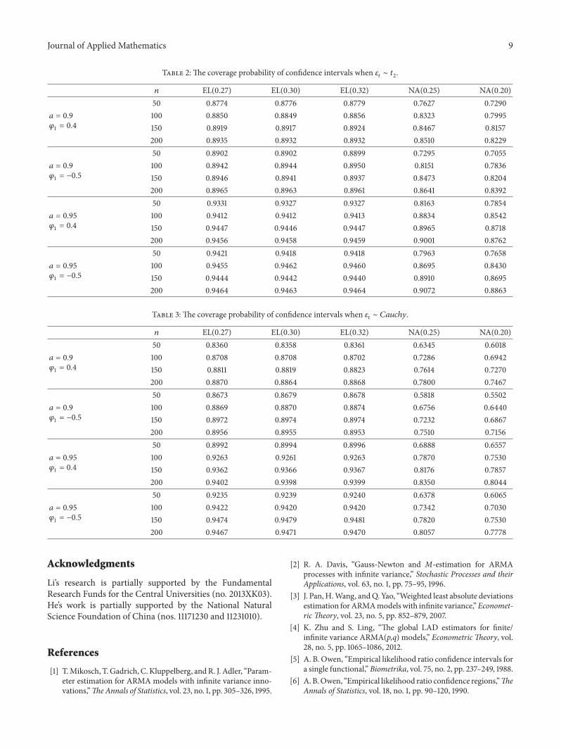