Active Filters - Circuits and Systemscas.ee.ic.ac.uk/people/dario/files/E22/L7-Active...

Imperial College London – EEE 1L7 Autumn 2009 E2.2 Analogue Electronics

Active FiltersMotivation:

• Analyse filters • Design low frequency filters without large capacitors• Design filters without inductors• Design electronically programmable filters


Some waveforms, to show the effect of filtering

Frequency domain Time domain

Noisy sine

Low Pass

High Pass

Band Pass

Band Reject


Filter typesLow pass High pass

Band pass Band Reject

Observe that a real filter is not sharp, and its transmission is not constant!


• Filters do not only change magnitude of signal• Filters alter phase as a function of frequency, i.e. introduce delays• The derivative of phase is a time delay• All pass filters delay signals without affecting their magnitude• All pass filters can be used to synthesise other filters:

• All pass filter based analogue filters are similar to the digital filters encountered in Digital Signal Processing

All Pass Filters

APF APF APF

c1

+

c2

+

c3

+

c4

Input

Output

Delay elements

Coefficients


The transfer function

• The transfer function is the Fourier transform of the impulse response• Filters we can make have a rational transfer function: the transfer

function is is a ratio of two polynomials with real coefficients. (strictly speaking this is called the “Padé approximation”: it states that any real function can be approximated by a rational function. The higher the degree of the polynomials the closer the approximation can be made) The notation is s=jω. The signals assumed to be sinusoid:

• The roots zk of the numerator polynomial are called the “zeroes” of H• The roots pk of the denominator polynomial are called the “poles” of H• The pole positions on the complex frequency plane entirely determine

the filter properties. • Note that since s=jω the denominator is seldom zero

( ) ( )( )

( )( ) ( )( )( ) ( )

1 20

1 2

0

nk

kn n nk

mkn m m

kk

a sP s a s z s z s zH s

Q s b s p s p s pb s

=

=

− − −= = =

− − −

∑

∑

0j tV V e ω φ+=


Families of filters• Filters are classified into different families according to how the

passband, stop band, transition region and group delay look like.• Most filters you are likely to encounter have a low pass power transfer

function of the form :

• Pn is a suitable polynomial, or a polynomial approximation to somedesired function. Pn are tabulated in reference books.

• Some common filter families (determined by Pn,) are:– Butterworth. Maximally flat pass-band, slow transition to stop band– Chebyshev: Fast transition at the cost of pass-band ripple– Inverse Chebyshev: Fast transition at the cost of stop-band ripple– Elliptic: Fastest transition at the cost of ripple everywhere– Bessel: Maximally flat group delay (almost linear dependence of

phase on frequency)• HPF, BPF, BRF, APF can be derived from a low pass prototype (next)• Note that a fast passband - stopband transition results in a large

variation of delay with frequency, i.e. unsuitable for digital signals!

( ) ( ) ( )*

2 2

11 n

H s H sP sε

=+


Pole-zero plots of Low Pass Filters

Pole locations determine filter response. The closer poles are to the imaginary axis the steepest the transition from passband to stopband.a: Butterworth: poles on a circleb: Chebyshev: Poles on an ellipse (sharper)c: Elliptic: Like Chebyshev, plus zeroes on the imaginary axis (sharpest)

dario

Rectangle

dario

Rectangle

dario

Rectangle

dario

Rectangle

dario

Rectangle

dario

Rectangle

dario

Rectangle

dario

Rectangle

dario

Rectangle

dario

Rectangle


• Write the desired transfer function.• Find Z(s) so that the following voltage divider is equal to the transfer function.

Passive filter synthesis

( ) ( )( ) ( ) ( ) ( )1 1 1 11

outs L

in Ls L

vH s Z s R Gv G H sZ s R G

⎡ ⎤= = ⇒ = − +⎢ ⎥

+ + ⎣ ⎦• Use R,L,C to implement Z(s); • Rs and YL are assumed known, usually real. The ideal cases Rs=0, YL=0 are trivial• If Rs and Ys are not real we can add and subtract their imaginary parts from Z(s)• There are many ways to make Z(s)• We prefer “canonical forms”, which use least number of components• We commonly use “Cauer forms” which are canonical ladder networks.

Z(s)Vin

Vout

GL

Rs


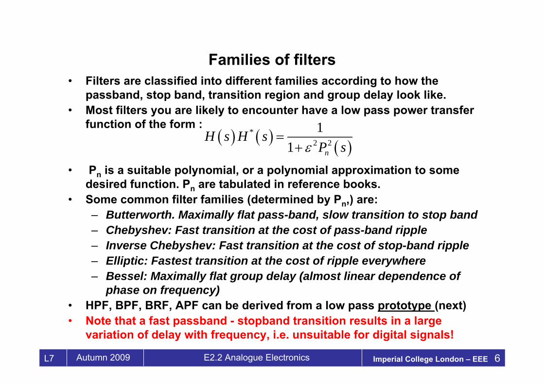
L1 L2 L3 Ln

L1C1 CnC1 L2C2 C3

LnCn

C2

(b)(a)

Cauer forms

Cauer forms are derived by a continued fraction expansion of Z(s):

First Cauer form Second Cauer form

3

2 2

2 111 1

s s ss ss s s

s

+= + = +

+ + +Or, we can start from the Z-function:

1

1

2

11

1inZ sL

sCsL

= ++

+

For the circuit on the left


2nd order filter transfer functions: ReviewSecond order filter transfer functions are all of the following form:

H0 is the overall amplitude, ω0 the break (or peak) frequency, and ζ the damping factor

ζ is related to the quality factor Q by: Q=1/2ζ

The 3dB bandwidth of an underdamped 2nd order filter is approx 1/Q times the peak frequency.

The coefficients A, B, C determine the function of the filter:

( ) ( )( )

20 0

0 20 0

/ 2 / 1 , 2/ 2 / 1

C s B s AH s H Q

s sω ζ ω

ζω ζ ω

+ += =

+ +

1-11All Pass101Band Stop010Band Pass100High Pass001Low PassCBAFunction

2nd order filters are useful: we can always decompose higher order filters to acascade of 2nd order filters!


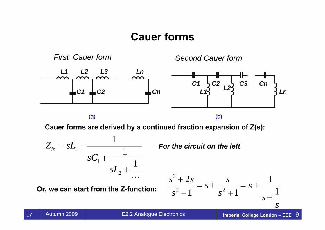
( ) ( ) ( ) ( )= , yj t st j t stx X e X s e Y e Y s eω ωω ω= = =

Filters solve differential equations

Substitute:

To get:

( ) ( )( )

( )( )

2

0 2

/ 2 // 2 / 1

n n

n n

Y s C s B s AH s H

X s s sω ζ ω

ω ζ ω

+ += =

+ +This is the transfer function of a 2nd order filter. It follows that the filter solves the ODE.

The impulse responses (IR) of lowpass, bandpass and highpass filters are related*:

• The IR of the BP is proportional to the time derivative of the IR of the LP • The IR of the HP is proportional to the time derivative of the IR of the BP• It follows that a loop of 2 integrators can implement any 2nd order filter. Such a loop is called a “biquad”.

* (remember that H(s) is the Laplace transform of the impulse response)

Consider the ODE:

( ) ( )2 2

02 2 2 2

1 2 21n n n n

d d C d dy t H B A x tdt dt dt dt

ζ ζω ω ω ω⎛ ⎞ ⎛ ⎞

+ + = + +⎜ ⎟ ⎜ ⎟⎝ ⎠ ⎝ ⎠


Filter transformations: LP HP

From a 2nd order low pass filter we can get a 2nd order high pass filter:

( )

( ) ( )

02

20

2

let / then for a 2nd order LPF:

2 1

1/1 2

n

LP

LP HP

q jHH q

q qH qH q H q

q q

ω ω

ζ

ζ

=

=+ +

= =+ +

If the components of a filter are replaced so that any impedancedependence on ω is replaced by a similar dependence on 1/ω the filter changes from low pass to high passIn practice we replace C with L and L with C so that:

1n

n

CL

ωω

=

The same transformation generates a low pass filter from a high pass filter.


Filter transformations LP BP

From a 1st order low pass filter we can get a 2nd order band pass filter:

( )

( ) ( ) ( )

0

0 01 22

let / then the transfer function of a 1 order LPF is:

1/1/ 1

stn

BP

q jHH q

a qH H qH q q H q

a q q q aq

ω ω=

=+

+ = = =+ + + +

In practice we replace the low pass elements, following the following recipe:• all capacitors with parallel LC circuits, (open at resonance) and • all inductors with series LC circuits (short at resonance)

1n

n

CL

ωω

=

ωn is the centre frequency of the filter. The BPF has the same BW as the LPF

,4 2n n B LPFf fδ πζω παω= = =To get a band reject filter replace in the low pass prototype:C series LCL parallel LC


Filter design from prototypesTabulated filter prototypes are usually given for low pass filters, with break frequency 1 rad/s and load impedance 1 ohm

From a LP filter prototype to get a HP filter with the same break frequency by the mapping: f 1/f.

• replace C with L and L with C• component values so that new components have same Z as old. • for a 1rad/s prototype this means C 1/L, L 1/C

From a LPF we get a BPF of bandwidth equal to the low pass bandwidth by:

• Replacing each L with series LC resonating at ωn. L stays the same• Replacing each C with parallel LC resonating at ωn. C stays the same• Choosing the undetermined components to resonate at the filter centre frequency product

From a high pass ladder LC filter we get a band-stop filter by applying the same recipe as going from low-pass to band-pass.

These rules arise from requiring components to have the required impedance at important points of the frequency response: The centre frequency and the band edge. (Remember that a LPF is a BPF centred at f=0!)


Filter design from Ladder prototypes: component scalingTo scale the filter so it works at the required impedance level Z0 ohms:

To scale a low pass so that its break frequency is the required f0 Hz:

After these transformations we can use the transformations from low pass to the required filter function as described before

0 0 , C f C L f L′ ′= =

0 0/ , C C Z L Z L′ ′= =

Note: it is unusual to treat signal sources as pure voltage or current sources in professional engineering applications. (This would make circuits too noisy!)In professional audio the standard impedance used is 600 Ohms.In cable, video and television applications the standard is 75 ohms In most other radio frequency applications the standard is 50 ohms.


(a)

R

Vin

C

Vout

(b)

R

Vin

C

Vout

R11st order low pass filter: the “Integrator”

1vA

RC−

=

“ideal” integrator Lossy integrator

Note: The ideal integrator is unstable at DC, and can only be used inside a feedback loop

With ideal op-amp:

1

1

11v

RAR j R Cω−

=+


(a)

Vin Vout

(b)

R1

Vin Vout

C

R

C

R

1st order high pass filter: the “differentiator”

Ideal differentiator Lossy differentiator

Note: The ideal differentiator when implemented with real op-amps becomes a very sharp Band Pass filter (lab, homework exercise)!


R1

Vin

C2

Vout

R2

C1

A simple band pass filter

Band pass filters are often a cascade of an LPF and an HPF,In this example the op-amp acts both as a differentiator and an integrator.


2nd order low pass passive RC filterR1 R2

C1 C2Vin

Vout

• Since the minimum value of x+1/x is 2• It follows that passive RC 2nd order filters are OVERDAMPED• The passive band pass filter transfer function calculation is part of experiment “Y” in the lab.• Easiest way to analyse ladder networks is to construct successive Thevenin equivalent circuits starting from the source.

( ) ( ) ( )2 21 1 2 2 1 1 2 2 1 2 1 2 1 2 12

1 2 120 1 2

2 1 21

1 11 1

1 11/ , 2 = = 2Q 2

H ss R C R C s R C R C R C s s

Q

τ τ τ τ τ

τ τ τω τ τ ζτ τ τ

= =+ + + + + + + +

= + + > ⇒ <


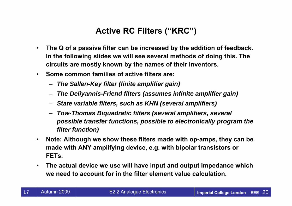
Active RC Filters (“KRC”)

• The Q of a passive filter can be increased by the addition of feedback. In the following slides we will see several methods of doing this. The circuits are mostly known by the names of their inventors.

• Some common families of active filters are:– The Sallen-Key filter (finite amplifier gain)– The Deliyannis-Friend filters (assumes infinite amplifier gain)– State variable filters, such as KHN (several amplifiers)– Tow-Thomas Biquadratic filters (several amplifiers, several

possible transfer functions, possible to electronically program the filter function)

• Note: Although we show these filters made with op-amps, they can be made with ANY amplifying device, e.g. with bipolar transistors or FETs.

• The actual device we use will have input and output impedance which we need to account for in the filter element value calculation.


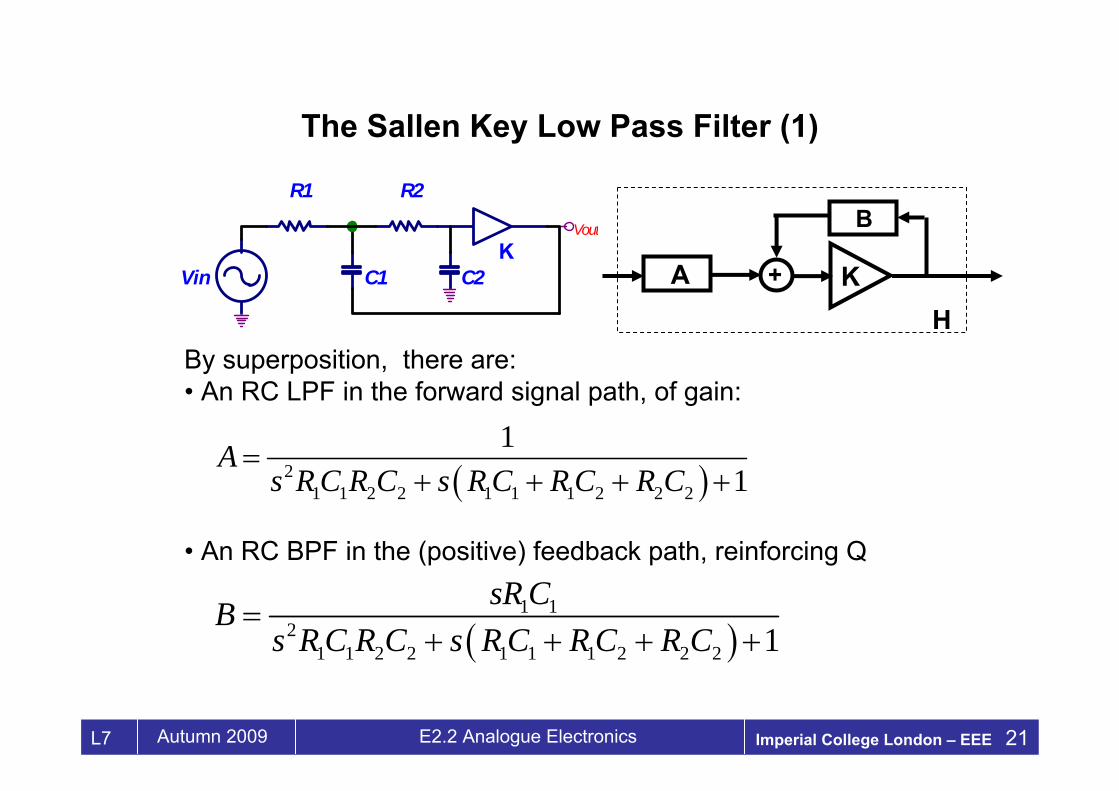
The Sallen Key Low Pass Filter (1)

R1 R2

C1 C2Vin

VoutK

By superposition, there are:• An RC LPF in the forward signal path, of gain:

• An RC BPF in the (positive) feedback path, reinforcing Q

( )21 1 2 2 1 1 1 2 2 2

11

As R C R C s R C R C R C

=+ + + +

( )1 1

21 1 2 2 1 1 1 2 2 2 1

sR CBs R C R C s R C R C R C

=+ + + +

A K

B

H+


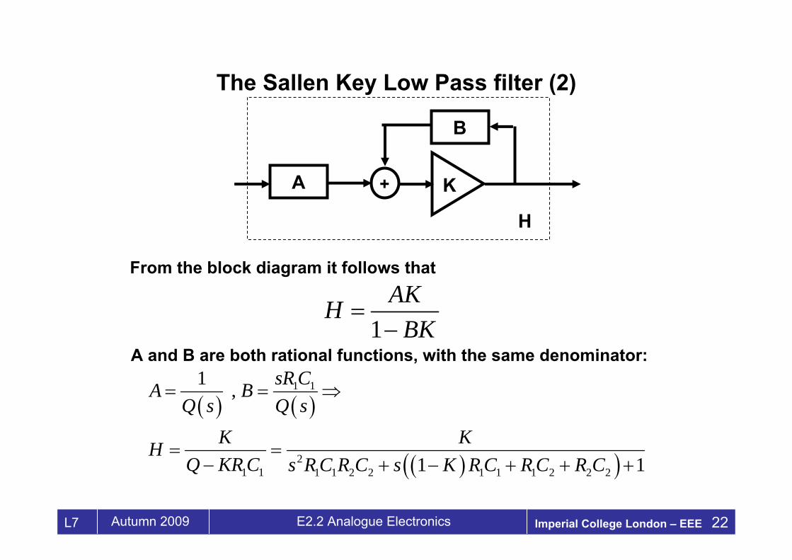
The Sallen Key Low Pass filter (2)

1AKH

BK=

−

A K

B

H

+

From the block diagram it follows that

A and B are both rational functions, with the same denominator:

( ) ( )

( )( )

1 1

21 1 1 1 2 2 1 1 1 2 2 2

1 ,

1 1

sR CA BQ s Q s

K KHQ KR C s R C R C s K R C R C R C

= = ⇒

= =− + − + + +


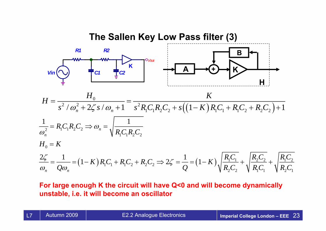
The Sallen Key Low Pass filter (3)

A K

B

H+

R1 R2

C1 C2Vin

VoutK

( ) ( )

1 1 2 221 1 2 2

0

1 1 2 2 1 21 1 1 2 2 2

2 2 1 1 2 1

1 1

2 1 11 2 1

nn

n n

R C R CR C R C

H K

R C R C R CK R C R C R C KQ Q R C R C R C

ωω

ζ ζω ω

= ⇒ =

=

= = − + + ⇒ = = − + +

For large enough K the circuit will have Q<0 and will become dynamically unstable, i.e. it will become an oscillator

( )( )0

2 2 21 1 2 2 1 1 1 2 2 2/ 2 / 1 1 1n n

H KHs s s R C R C s K R C R C R Cω ζ ω

= =+ + + − + + +


The Sallen Key High pass filter

C1 C2

Vin

Vout

R1 R2K

By superposition, there are:• An RC HPF in the forward signal path• An RC BPF in the (positive) feedback path, reinforcing Q• Analysis very similar to that of the SK-LPF• Detailed calculation left as a homework problem

A K

B

H+


The Sallen Key Band pass filter

C1

C2

Vin

VoutR1

R2

R3

K

This has identical in form passive band pass filters in the forwardand feedback paths, shown on the middle. The block diagram in theright is the same form as the other SK filters. If R1=R3 then the twofilters are identical and A=B . The transfer function of each path filter is:

( )2

1 1 1 2 2 2 12 1 221 2 2 1 12

, , ,2 2

sA B R C R C R Cs s

τ τ τ ττ τ τ τ τ

= = = = =+ + + +

The entire SK filter has a transfer function:

A K

B

H+

( )( )2

21 2 2 12 1

/ 21 / 2 2 / 2 1

KsAHHAH s K s

ττ τ τ τ τ

= =− + − + + +

This circuit is studied in exercise 4 of the lab experiment ”Y”.


The Sallen Key Notch filter

Vin

Vout

2C

C C

R

R/2

R

K

A K

B

H

+

A B

Networks A, B may be solved by nodal analysis or any other suitable method.


Multiple feedback filters: “Deliyannis-Friend” (“DF”)

• Op-amp is ideal• Inverting input is virtual GND, V=0, i=0• Nodal analysis usually simple•Tee-Pi transforms may simplify algebra

Low Pass Band Pass

All Pass


“State Variable” filters - KHN

• “state variable filters” treat both the signal and its derivatives as variables • A low pass filter performs time integration on signal waveforms• A high pass filter performs time differentiation on signal waveforms• Recall that filters are analogue computers which solve ODEs


“State Variable” filters – KHN : analysis

• Block A is a weighted sum amplifier• Blocks B and C are integrators• Some maths: (after we get the constants K1 , K2, K3 by nodal analysis)

A x

B C

yz

1 21 2 3

2 1 22

1 2 32

2 3 1

2 / / , , 1/ /

,

(low pass filter) (Block C is an integrator, y is a BPF output) (Block B is an integrator, x is a HPF

i

i

R RRC K K KR R R

x K v K y K z x y z

z K z K z K vy zx y

τ

τ τ

τ τττ

= = = = −+

= + − = − = ⇒

− + == −= − output)


Another state variable filter: the Tow-Thomas “Biquad”

• the term “Biquadratic” or “Biquad” describes the 2nd order filter transfer function as a ratio of two quadratic polynomials • R1, R2, R3 act as logical switches. Their presence or absence determines the filter function as Low, High or Band Pass • This is a single output universal filter; its function can be switched.• The Tow Thomas filter an be treated:

• By nodal analysis (easiest) or• As a “state variable” filter (note the two integrators and the summing operators )


Higher order filter synthesis using 2nd order sections• A general filter transfer function is of the form:

• P(s) and Q(s) have real coefficients. To make a higher order filter:– factor Q(s) into quadratic and linear factors– Implement factors as biquads– Cascade biquad sections to obtain the original transfer function– Note that P and Q have real coefficients, so that their roots are either

real or come in conjugate pairs.• The centre frequencies and damping factors of the sections required to

implement standard forms (Butterworth, Chebyshev, Elliptic etc) are tabulated in reference books.

• Tables are also included in CAD software for automated filter synthesis

( ) ( )( )

( )( ) ( )( )( ) ( )

0 10

0 1

0

nk

kn ni

mkm n

ki

a xP s s z s z s zH s

Q s s p s p s pb x

=

=

− − −= = =

− − −

∑

∑


A useful network transformation: Impedance inversion and the gyrator

A gyrator can perform• impedance inversion (L C)• Impedance scaling• series parallel connection conversion!

“Proper” symbol of gyrator

Alternate symbolSimple active implementation (very popular by analogue CMOS designers.Each gm is made of a MOSFET or two!)


Passive Gyrators

• ¼ wavelength transmission line

• Pi and Tee networks with negative elements

negative values of components will be added to preceding and subsequent stage impedances resulting in overall positive impedances!

Ladder LC filters can be synthesised only with capacitors and gyrators

Z, -Z is completely arbitrary, can be a filter transfer function.


•Two identical gyrators in series are the identity operator

•Two different gyrators in series form a transformer, i.e. perform impedance scaling.

Gyrator function - basics

• A series (floating) component between two gyrators appears gyrated and grounded

• A grounded component between two gyrators appears gyrated and in series


More gyrator identities

how to make e.g. a series resonance circuit when you only have parallel resonators in your component box… and vice versa


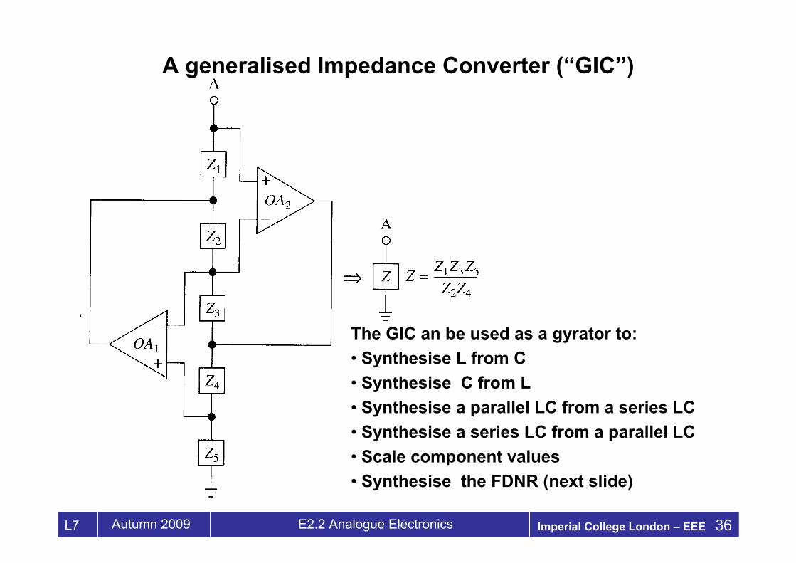
A generalised Impedance Converter (“GIC”)

The GIC an be used as a gyrator to:• Synthesise L from C• Synthesise C from L• Synthesise a parallel LC from a series LC• Synthesise a series LC from a parallel LC• Scale component values• Synthesise the FDNR (next slide)


FDNR: the frequency dependent negative resistor• The filter transfer function of a circuit does not change if all components are multiplied by a constant K•There is no requirement that the constant K is frequency independent!• A useful multiplicative constant is

which• Transforms R C• Transforms L R• C FDNR

• FDNR is a fictitious circuit element with:

•A GIC can be used to implement an FDNR as illustrated on the right• FDNR filters is one possible implementation of inductorless filters

2Y Dω=−

1/K jωτ=


Example of FDNR transformation

Note that we can scale the filter coefficients by any factor of our choice, including jω. All we need is that the voltage divider works as intended at all frequencies!


Switched Capacitor Filters: introduction

C

S1 S2

V1 V1

I R

(a) (b)

V2 V2

C

S

V S

S1

S1

Vout=-V

CSV

Vout=2V

CS1S1

S

(a) (b)

•(a) And (b) circuits are equivalent as long as signal frequency is much smaller than switching frequency•The SC equivalent resistance is proportional to frequency

• Switched Cap circuits can be used for voltage amplification • Switched Cap voltage amplifiers are called “charge pump” circuits• examples of charge pump circuits: (a) V-gain=-1 , (b) V-gain=2


Switched Capacitor Biquads

• Commercial chips contain several (typically 4) SC biquads in a package, which are then programmed and cascaded to synthesise higher order filters• Frequencies of operation beyond audio (20kHz), typical constraint is product of fo and Q. Switching frequenies in the MHz (need > 10x of highest f)• This example has a structure similar to the Tow-Thomas

Summing junctionInvertingLossy integrator Inverter

InvertingIdeal integrator


Beyond KRLC: high Q filters

• Crystals. They behave in a circuit as series or parallel LC resonators:– “Series mode” show an impedance minimum at resonance– “Parallel mode” show an impedance maximum at resonance– Quality factors very high– Low temperature variation, if necessary stabilised with “oven”

• Dielectric Resonators– A magnetic ceramic bead placed near a coil– Dimensions of bead determine frequency of resonance

• Surface acoustic wave filters– Printed conductor patterns on piezoelectric crystals– Filter function synthesised by interference of surface piezoelectric

waves coupled to printed electrodes– Filter function extremely sensitive to source-load impedance


Summary

• Types of filters: LP, HP, BP, BR, AP• Transfer functions• Bode Plots review• Lumped element synthesis – Ladder filters• Prototypes and transformations• 1st order filters• 2nd order filter transfer function• Active filters: SK, DF, KHN, TT• Gyrators and Generalised Impedance Converters• Introduction to Switched capacitor filters

Active Filters - Circuits and Systemscas.ee.ic.ac.uk/people/dario/files/E22/L7-Active...

Documents

Transcript of Active Filters - Circuits and Systemscas.ee.ic.ac.uk/people/dario/files/E22/L7-Active...