ABSTRACT

Title: DEVELOPMENT OF AN OFF-LINE RAINFLOW COUNTING

ALGORITHM WITH TEMPORAL PARAMETERS AND DATA

REDUCTION

James M. Twomey, 2016

Directed by: George E. Dieter Professor, Michael G. Pecht,

Department of Mechanical Engineering

Rainflow counting methods convert a complex load time history into a set of load

reversals for use in fatigue damage modeling. Rainflow counting methods were originally

developed to assess fatigue damage associated with mechanical cycling where creep of

the material under load was not considered to be a significant contributor to failure.

However, creep is a significant factor in some cyclic loading cases such as solder

interconnects under temperature cycling. In this case, fatigue life models require the

dwell time to account for stress relaxation and creep.

This study develops a new version of the multi-parameter rainflow counting

algorithm that provides a range-based dwell time estimation for use with time-dependent

fatigue damage models. To show the applicability, the method is used to calculate the

life of solder joints under a complex thermal cycling regime and is verified by

experimental testing.

An additional algorithm is developed in this study to provide data reduction in the

results of the rainflow counting. This algorithm uses a damage model and a statistical test

to determine which of the resultant cycles are statistically insignificant to a given

confidence level. This makes the resulting data file to be smaller, and for a simplified

load history to be reconstructed.

DEVELOPMENT OF AN OFF-LINE RAINFLOW COUNTING ALGORITHM WITH

TEMPORAL PARAMETERS AND DATA REDUCTION

By

James M .Twomey

Thesis submitted to the Faculty of the Graduate School of the

University of Maryland, College Park in partial fulfillment

Of the requirements for the degree of

Master of Science

2016

Advisory Committee:

Professor Michael G. Pecht, Chair

Professor Abhijit Dasgupta

Doctor Diganta Das

Doctor Michael D. Osterman

© Copyright by

James M. Twomey

2016

ii

Acknowledgements

I wish to express my thanks to all who have supported this work. I thank Dr.

Michael Osterman and Prof. Michael Pecht for providing advice and direction to this

project and for the work they put into reviewing my papers and software. Additionally, I

am thankful to the rest of the CALCE staff and students for the helpful comments and

suggestions they provided along the way, including Dr. Diganta Das, Prof. Abhijit

Dasgupta, Dr. Michael Azarian, and Dr. Carlos Morillo along with the rest of the

morning meeting group. Finally, I would like to express my gratitude for the support and

encouragement of my girlfriend, An Thai; my sister, Prof. Kelly Sanders; and my parents,

Matthew and Mary Twomey.

iii

Contents Chapter 1: Rainflow Counting .........................................................................................1

1.1 Damage Modeling ..................................................................................................6

1.2 Damage Summation ...............................................................................................8

1.3 Probabilistic Modeling ...........................................................................................9

1.4 Overview of Thesis .............................................................................................. 14

Chapter 2: Literature Review ......................................................................................... 14

2.1: Multi-parameter Rainflow Algorithms ................................................................ 14

2.2: Data Minimization .............................................................................................. 18

2.2.1 Minimizing the Original Time History .......................................................... 18

2.2.2 Low-pass filters ............................................................................................. 19

2.2.3 Range threshold filtering ............................................................................... 21

2.2.4 Damage exponent based reduction................................................................. 22

2.2.5 Damage estimate reduction-based reduction .................................................. 23

2.2.6 Binning ......................................................................................................... 23

Chapter 3: New Multi-parameter Rainflow Counting ..................................................... 24

3.1 Proposed Algorithm ............................................................................................. 26

3.2 Comparison to prior methods ............................................................................... 37

3.2.1 Comparison of Dwell Estimates .................................................................... 46

3.2.1 Comparison of Damage Estimates ................................................................. 53

iv

3.3 Stability of Damage Estimates in the Proposed Algorithm.................................... 58

3.4 Stability over sampling rates ................................................................................ 59

3.5 Stability over history length ................................................................................. 61

3.6 Comparison of Run times and Memory Requirements .......................................... 63

Chapter 4: Automated Cycle Reduction ......................................................................... 64

4.1 Proposed Algorithm ............................................................................................. 65

4.2 History Reconstruction......................................................................................... 67

4.3 Demonstration of Automated Cycle Reduction and Reconstruction ...................... 69

5. Conclusions ............................................................................................................... 72

4.1 Contributions ....................................................................................................... 73

A multi-parameter rainflow counting algorithm was developed and implemented to

estimate dwell time using monotonic data and retain cycle timestamps. ..................... 73

4.2 Suggested Future Work ........................................................................................ 74

Works Cited .................................................................................................................. 75

v

List of Tables

Table 1: Average dwell values ....................................................................................... 41

Table 2: Estimated Damage ........................................................................................... 44

Table 3: Damage Comparisons between Cluff and prosed dwell definitions ................... 45

Table 4: Damage estimates ............................................................................................ 59

Table 5: Data reduction comparisons ............................................................................. 72

vi

List of Figures

Figure 1: Rearranging the time series data and extracting a cycle. Adapted from [2] ........2

Figure 2: Closed loop extraction ......................................................................................4

Figure 3: Stability of a Monte Carlo output .................................................................... 13

Figure 4: Low pass filter on a time-temperature history ................................................. 20

Figure 5: Dwell time definition based on load range percentage ..................................... 27

Figure 6: Time removal illustration ................................................................................ 30

Figure 7: Flow chart for the proposed algorithm ............................................................ 33

Figure 8: Detailed flowchart for the half cycle extraction step ........................................ 34

Figure 9: Detailed flowchart for the dwell time calculation step ..................................... 35

Figure 10: Detailed flowchart for the data deletion step ................................................. 36

Figure 11: Each of the four data sets under consideration ............................................... 40

Figure 12: Average normalized dwell times for test profile (top) and the three remaining

estimates (bottom) ......................................................................................................... 42

Figure 13: Comparison to experimental data .................................................................. 44

Figure 14: Normalized damage estimates ....................................................................... 45

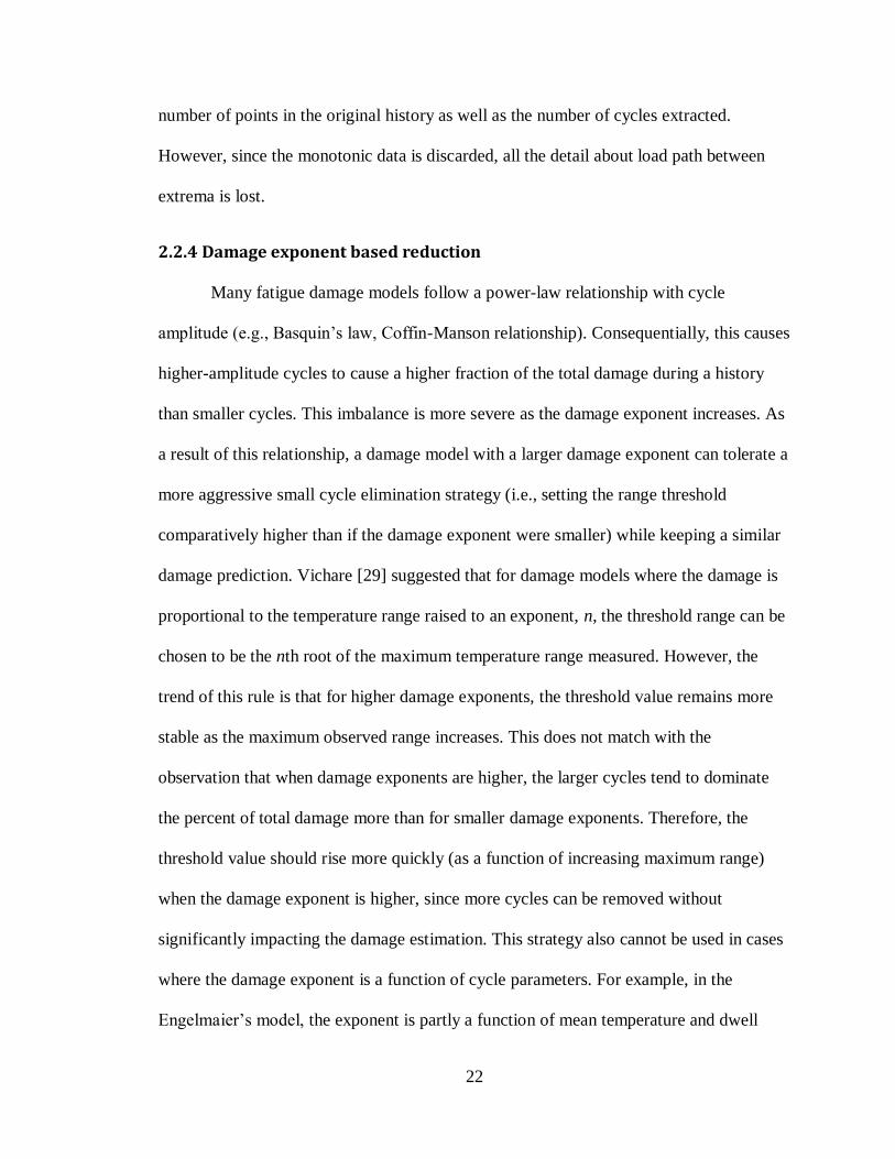
Figure 15: Stability of average dwell time for proposed and Vichare methods for test

profile data set ............................................................................................................... 47

Figure 16: Stability of average dwell time for proposed and Vichare methods for outdoor

data set .......................................................................................................................... 48

Figure 17: Distribution of dwell times for outdoor data set............................................. 49

Figure 18: Stability of average dwell time for proposed and Vichare methods for laptop

data set .......................................................................................................................... 50

Figure 19: Distribution of dwell times for laptop data set ............................................... 51

vii

Figure 20: Stability of average dwell time for proposed and Vichare methods for desktop

data set .......................................................................................................................... 52

Figure 21: Distributions of dwell estimates for desktop data set ..................................... 53

Figure 22: Damage comparisons for outdoor data set ..................................................... 55

Figure 23: Damage estimates for laptop data set ............................................................ 56

Figure 24: Damage estimates for desktop data set .......................................................... 57

Figure 25: Stability of damage estimates for each data set .............................................. 58

Figure 26: Stability of damage estimate over decreasing sampling rates ......................... 61

Figure 27: Stability of damage estimates over smaller history lengths ............................ 62

Figure 28: Run time comparisons .................................................................................. 64

Figure 29: Memory usage comparisons .......................................................................... 64

Figure 30: Example of reconstructed history for outdoor data set (top) and test profile

data set (bottom) ............................................................................................................ 68

Figure 31: Data reduction for outdoor data set ............................................................... 70

Figure 32: Data reduction for laptop data set .................................................................. 70

Figure 33: Data reduction for desktop data set ............................................................... 71

1

Chapter 1: Rainflow Counting

Fatigue in materials is caused by cyclically varying mechanical stresses. These

stresses may result from shock, vibration, thermal expansion coefficient mismatches

between joined materials, or thermal gradients within a material. To predict the life of a

component under fatigue, information about the load cycles (e.g., cyclic mean and

amplitude of the load cycle) are needed as inputs to a fatigue life model (e.g., Basquin’s

law, Coffin-Manson, Engelmaier’s model). This would assume that the load conditions

are constant, e.g., the load is cycling with a fixed mean and amplitude. However, in field

conditions, materials may experience loads in a more complex pattern than can be

parameterized in a single cyclic mean and amplitude. Therefore, there is a need for a

technique that transforms a complex load history to a format which can be input into

fatigue models. This transformation is achieved through “cycle counting.”

Cycle counting allows individual cycles to be extracted from a load history.

Cycles can be analyzed individually and aggregated through a damage summation rule,

such as Palmgren-Miner’s rule. This rule assumes that the percentage of life consumed by

a load can be simplified to the ratio of cycles experienced at that load to the number of

cycles to failure at that load. This allows multiple types of loads to be linearly summed.

When the sum reaches unity, a failure is predicted.

1

1k

i

i i

n

N

(0.0)

The most popular cycle counting algorithm for fatigue analysis in metals is

rainflow counting [1]. This technique extracts intermediate cycles from larger half-cycles

2

in an irregular load history. To begin a simple rainflow counting algorithm [2], the time

series load data first needs to be rearranged so that the history begins with either the

highest peak or the lowest valley. This makes the assumption that the load history can be

approximated as periodically repeating, as the end of the first history will be joined to the

start of the second history.

Next, consider the two load ranges formed by the next three local extrema. If the

first of these ranges is larger or equal to the second, the extraction criterion is met. If the

point under consideration is not the first point in the history, discard the second range and

count one cycle. If it is the first point in the history, delete that point and count one half

cycle. Else, if the extraction criterion is not met, move forward in the time series to the

Figure 1: Rearranging the time series data and extracting a cycle. Adapted from

[2]

3

next two load ranges, repeating until there is no more data or there is less than three peaks

or valleys left. This process is partially illustrated above in Figure 1.

This is a three-point rainflow algorithm, since the two ranges considered are

formed from three points. A four-point version of the algorithm can also be used [3]

(where the extraction criteria requires that the middle of three ranges are less than or

equal to the first and third), but this was proved to be equivalent to the three-point version

[4]. This is also an offline algorithm requiring the entire history to be known before

processing, although online versions have been proposed [5] [6].

There are other methods of cycle counting, including level-crossing counting,

peak counting, simple-range counting, and range-pair counting [2]. Level crossing

counting records every time a load crosses a defined threshold away from the neutral axis

(i.e., an increasing positive load or a decreasing negative load). These crossings are

assumed to be accompanied by corresponding load crossings towards the neutral axis.

These crossings could be equivalently counted instead. This can be used to reconstruct

full load cycles in a form useable for a damage model. Peak counting involves counting

each maximum and minimum in the data, then matching the peaks in order of largest

formed ranges to smallest. These matched peaks form individual cycles. Simple range

counting divides the load histories into half cycles at each local extrema, so the damage

modeling is simply applied to each half cycle.

4

Figure 2: Closed loop extraction

Rainflow counting is justified by assuming that closed loops in stress-strain space

can be analyzed independently [1]. For example, in Figure 2, the load time series history

experiences two load reversals. As shown on the stress-strain plot, the material deforms

in a linear elastic fashion the stress reaches yield stress σo. After yielding, there is non-

linear plastic deformation until the stress reaches the load reversal at σ’. The material

then unloads linearly up to a total stress range of 2σo (assuming this material exhibits

kinematic hardening behavior) before deforming plastically. At the next load reversal σ’’

the loading path is again linear elastic to a total stress range of 2σo. In the following

plastic deformation, the load path intersects the original curve at σ’. This loop-closing

behavior is known as the “memory effect.” Since this intersection forms a closed loop,

the loops are treated as independent. The inside loop is extracted during rainflow

counting and the larger loop is treated as continuous.

5

In one-parameter rainflow counting, only the ranges of the extracted cycles are

counted. In many cases, engineers may be interested in other parameters in addition to

load range. If a fatigue model also requires the mean of the cyclic load, the cycles are

binned into a matrix to record both the mean and the range of the load cycles. For

situations where the material experiences time-dependent damage mechanisms such as

creep or oxidation, the rainflow algorithm must also record temporal information (e.g.,

ramp rate, cycle period, dwell time). Three-parameter rainflow counting extracts range,

mean, and a temporal parameter such as dwell time.

When using rainflow counting for damage estimation on solder interconnects,

three-parameter rainflow must be used. This is because solder experiences significant

creep damage even at room temperature, so factors such as ramp rates and dwell times

can impact damage accumulation.

Thermal cycling can cause damage to solder interconnects in electronics as a

result of differing coefficients of thermal expansion (CTE) between an electronic

component (e.g., an integrated circuit) and the supporting printed wiring board (PWB) to

which it is soldered. These differing expansion rates cause shearing of the solder joints

during a thermal cycle, eventually leading to cracks propagating through the joints,

causing increases in electrical resistance across the connection or electrical opens.

Specification and life prediction for these types of failures often involve the

characterization of a usage profile involving one type of thermal cycle continually

repeated. For example, the IPC Guidelines for Accelerated Reliability Testing of Surface

Mount Solder Attachments [7] characterizes use environments as having a single

maximum temperature swing (although it does caution that actual use conditions “need to

6

be established by thermal analysis or measurement”). In reality, temperatures will

fluctuate irregularly, preventing the direct application of a fatigue life model (e.g.,

Engelmaier’s model).

1.1 Damage Modeling

Several models are available for estimating the life of solder interconnects during

thermal cycling. One semi-empirical model was initially developed in 1983 [8]. This

model was derived from the Coffin-Manson relationship with empirical corrections for

factors such as temperature, cycle frequency, and lead stiffness. The strain range term in

the original Coffin-Manson equation is replaced by an equation including temperature

cycle range. This model was eventually included into standards such as the IPC Guide for

Accelerated Testing of Surface Mount Assemblies (IPC-SM-785) [7], the IPC Design

Guidelines for Reliable Surface Mount Technology Printed Board Assemblies (IPC-D-

279) [9], and the IPC Design Guide for Performance Test Methods and Qualification

Requirements for Surface Mount Solder Attachments (IPC-9701).

This model defines cycles to failure, Nf, as:

1

1

2 2 '

c

f

f

N

(0.1)

In this equation, ε’f is the fatigue ductility coefficient, Δγ is the cyclic shear strain

range, and c is the fatigue plasticity exponent given by:

0 1 2

360ln(1 )sj

dwell

c c c T ct

(0.2)

7

Tsj is the mean solder joint temperature, and tdwell is the average dwell time at each

extreme. c0, c1, and c2 are model coefficients. These three model coefficients, along with

ε’f, are calibrated for a particular solder material. The cyclic shear range for a leadless

component is given by:

dFL T

h

(0.3)

F is an empirical “non-ideal” factor that attempts to account for second order effects.

This factor is dependent on the package type under consideration. For example, a CLCC

package typically has a reported F value between 0.7 and 1.2 [10]. Ld is the longest

distance to the neutral point of expansion. Δα is the difference in the coefficients of

thermal expansion between the component and the substrate. ΔT is the cyclic temperature

range, and h is the solder joint height. For leaded parts, the cyclic shear range is:

dFDL T

h

(0.3)

D is the lead displacement transmissibility [11], which accounts for lead stiffness.

There are several known caveats to using this model. First, it makes assumptions

about solder joints. Short solder joints have properties driven more by their intermetallic

formations rather than their solder [12]. It is also assumed that the solder joints are not

influenced by things such as underfill or corner staking, which can alter the stresses

experienced by the joints. Another caveat is with regard to local CTE mismatches. The

Engelmaier model considers global CTE mismatches, i.e., between the package and the

substrate that the solder provides a connection to. There is also a local mismatch between

the solder and the component as well as between the solder and the substrate. This is a

8

large concern when the global CTE mismatch is very small, such as when a ceramic chip

is mounted on a ceramic substrate. This may also cause issues in severe use environments

[13]. The next caveat is that the model is not intended for large temperature ranges.

Engelmaier [13] suggested that the model should not be used for temperature ranges that

cross the region from –20 to 20°C, because the dam age mechanisms shift. Evans [14]

suggests that the model is most appropriately used in a range of 0±100°C. An additional

caveat is a limitation on cycle frequency. At high frequencies where cycle times are less

than 2 seconds or with dwells less than 1 second, creep and stress relaxation damage will

be overestimated. Engelmaier suggests the direct application of Coffin-Manson in this

case [13]. The last commonly reported caveat is that the model does not address leaded

parts with high stiffness and large expansion mismatches [7]. This results in unexpected

levels of plastic deformation, which degrades the model’s predictions.

1.2 Damage Summation

After the damage resulting from individual extracted cycles is determined, a

mechanism is needed that can sum this damage. The most popular tool for this task is the

Palmgren-Miner rule, also known as Miner’s rule. Miner’s rule is a linear damage

summation rule often applied to fatigue analysis under variable amplitude loading

conditions. The advantages of this rule include its ease of use, while the disadvantages

include its assumption of damage independence. In reality, materials may exhibit cyclic

hardening or softening over the course of the damage history, thus impacting the damage

accumulation rate. Additionally, harsh loads early in the damage history cause periodic

overstrain and may also make the sample more susceptible to damage later in the history.

9

While this method can give a large spread in accuracy, more sophisticated damage

summation rules require empirical data to calibrate.

1.3 Probabilistic Modeling

When a model gives a single value as an output rather than a probability

distribution, it is a deterministic prediction. However, this ignores uncertainty.

Uncertainty in damage prediction can come from several sources. For example,

uncertainty in damage prediction of solder joints could result from variations in geometry

of the specimen in question (e.g., as a result of manufacturing variations or defects) [14]

[15] or variations in material properties (e.g., as a result of microstructural evolution over

the life of the test). There is also uncertainty in the representation of the original load

history. In a recorded time series history, sources of uncertainty can include noise in

sensor measurements or potential error resulting from the sampling rate. If this analysis is

being used to inform a design, or being used for life prediction, there is uncertainty in the

usage conditions. For example, the sample load history may not exactly match history

experienced by the system in the field.

One way to attempt to quantify uncertainty is to perform a Monte Carlo

simulation, treating all model inputs (geometry factors, materials factors, loads and model

constants) as random variables. If probability distributions for each uncertain input

parameter into a model can be estimated, the distributions can be randomly sampled.

These samples can then be input into the model. This can be repeated until there are

enough samples to characterize the output distribution. This way, the uncertainty in the

modeling results is estimated.

10

The input distributions can be estimated using historical data. In the case of

rainflow counting, cycles are extracted from the time series history which results in a data

vector for each parameter, (i.e., cyclic mean, range, dwell time). These data vectors

resulting from the rainflow counting can be used to estimate probability distributions

[16]. There are parametric and non-parametric methods to estimate probability

distributions based on historical data.

Parametric methods require fitting the data is fit to a known parametric

distribution (e.g., normal, lognormal, or Weibull distributions). The suitability of this

strategy depends on how closely the data matches the choice of distribution. If the

underlying distribution being estimated is non-standard (e.g., multi-modal), there will be

a bias in the estimation. Non-parametric methods include histograms and kernel density

estimation. Histograms simply count occurrences of data points within a bin range,

forming a discrete distribution. Kernel density estimation provides a smoothed estimation

(compared to a histogram) by weighting the points (within a bandwidth h) around each

sample according to a parametric kernel function K.

1

1ˆ ( )n

j

h

j

x xf x K

nh h

(1.31)

Commonly used kernel functions include normal, uniform, triangular, and

Epanechnikov. While the local weighting function for each point is parametric, the total

probability distribution formed by the sum of the local functions is not, because the

kernel function is simply being used as a smoothing function around samples rather than

to structure the entire estimated distribution. If the parameter being estimated needs to be

11

bounded (e.g., if a parameter cannot be negative), the estimates near the boundaries may

be biased. Corrections can be applied to alleviate this issue [17]. This can be a problem

when estimating a parameter such as dwell time or cyclic range, since many samples may

be within the kernel bandwidth of zero, but negative values of these parameters are

impossible.

The suitability of a non-parametric estimation technique depends on how

comprehensively the observed data characterizes the underlying distribution. In higher

dimensions, non-parametric estimation techniques suffer from the curse of

dimensionality, since sample data tends to be more sparse (i.e., under-sampled) in higher

dimensional space. As a result of data sparsity, non-parametric estimations tend to have

higher variances compared to parametric techniques.

In using histograms, a bin width must be selected to form the range into which

data is counted. If the bin width is too large, the distribution is over-smoothed. In this

case, the details of the underlying distribution are lost. If the bin width is too small, the

distribution is under-smoothed. In this case, the noise in the data is over represented,

distorting the estimation of the underlying distribution. The bin width should be

optimized so that the histogram is neither under- nor over-smoothed. To calculate optimal

bin width for normally distributed data, the Scott rule [18] can be used:

* 1/33.49nh sn

(1.32)

For non-Gaussian data, the Freedman-Diaconis rule [19] can be used:

* 1/32( )nh IQR n

(1.33)

12

The analog to bin width in kernel density estimation is bandwidth. This is the width from

a data point where the distribution is weighted by the data point’s kernel function.

Optimal bandwidth for kernel density estimation can be calculated with the following

formula [16]:

1

5ˆ1.06opth sn

(1.34)

In order for the result of the Monte Carlo simulation to be realistic, correlations between

input variables should be considered in order to only generate meaningful data samples

[20]. For example, if cycles with at high temperatures only occur with small amplitudes,

then a high temperature should not be sampled with a large amplitude during the same

Monte Carlo iteration. This correlation can be modeled in several ways. A simple way to

create a dependency structure is fitting a parametric model that treats a variable as a

function of the variables it is correlated with (e.g., with a linear function). Other options

include rank order correlation [21], standard normal transformation [22] and copulas [23]

[24]. The optimal method depends on the data. In the thermal cycling profile used by

Chai [25], the extracted parameters are rigidly correlated as a result of the limited number

of cycle types in the profile. Therefore, sampling one variable (e.g., dwell time) and

treating the others (e.g., mean temperature and temperature range) as dependent variables

is adequate for simulating this history.

After each Monte Carlo iteration, the cumulative average output is calculated.

When this value becomes stable as a function of iteration number, the simulation is

complete (as illustrated in Figure 3). This stabilization can also be analyzed in terms of

13

the Standard Error (SE) of the Mean formula, in terms of sample standard deviation 𝜎 and

sample size n:

𝑆𝐸 =𝜎

√𝑛 (1.35)

The simulation can be stopped when the standard error reaches 1% of the mean (i.e.,

SE≤0.01µ). The cumulative average output value should approximately match the

deterministic model prediction, if one is available.

Figure 3: Stability of a Monte Carlo output

Rather than randomly sampling correlated distributions, other sampling methods

can be used for a Monte Carlo analysis. In cases where the sampling probability depends

entirely on the preceding state of the system, Markov chains can capture this dynamic

that would otherwise be ignored by random sampling. Data which exhibits

autocovariance can be modeled with an autoregressive (AR) model.

14

1.4 Overview of Thesis

This thesis aims to develop a rainflow counting method which is sensitive to

temporal parameters such as dwell time and cycle start time, as well as a data reduction

method to reduce the file size of the results and allow for a simplified load history to be

reconstructed. Chapter 1 provides an introduction into standard rainflow counting, a

dwell-time sensitive fatigue damage model for solder interconnects, as an introduction to

damage summation and probabilistic damage modeling. In chapter 2, the literature

relevant to time-parameter sensitive rainflow counting, as well as data reduction

techniques used with rainflow counting, is reviewed. Chapter 3 develops and analyzes the

new version of rainflow counting which uses a load range-based definition of dwell time,

in addition to extracting range, mean, and half-cycle start time. Chapter 4 develops and

analyzes an automated data minimization strategy which reduces the size of the rainflow

results using a damage model and a statistical test, allowing a unique simplified history to

be reconstructed. The conclusions, contributions and suggested future work of this thesis

are given in Chapter 5.

Chapter 2: Literature Review

2.1: Multi-parameter Rainflow Algorithms

When using rainflow counting for damage estimation on solder interconnects,

three-parameter rainflow counting is used, because solder experiences time-dependent

creep damage even at room temperature, and the ramp rates and dwell times can impact

damage accumulation. Cluff [26] and Denk both [27] implemented a three-parameter

15

rainflow algorithm which recorded the half cycle period formed within the range under

consideration.

Cluff’s three parameter rainflow method first simplified the history into peaks and

valleys. Next, cycles are under the same criteria as a standard 3-point rainflow method [2]

(the range under consideration must be less than or equal to in magnitude to the

preceding range). The peak temperature and the temperature range are discretized to 2°C

intervals and recorded, and the dwell time is taken to be 50% of the half cycle time,

regardless of the actual load path between the two points. The dwell was discretized to 12

minute intervals (based on the recording interval of the logging equipment). Therefore, a

quarter of the assumed full cycle time would be counted as dwell time. Three passes of

the algorithm were made before the remainder of the history was counted using simple

range counting (i.e., counting half cycles sequentially). This algorithm recorded only full

cycles, but during simple range counting, half cycles did not exactly match up. It was

assumed that positive half cycles can be combined with the closest, but smaller, negative

cycles” to be counted as a full cycle, then simply counting the remaining half cycles as

full cycles. The justification for doing this is that both assumptions provide conservative

estimates. Denk’s algorithm used standard rainflow counting [2] along with recording the

“heating time” of each cycle between the first and second extrema in the extracted cycle.

Both of these algorithms calculate the time elapsed during the extracted range, but

record full cycles. An improvement would be to independently interpolate the time length

of the second half of the cycle. Nagode [28] developed an online temperature-modified

cycle counting algorithm. Amzallag’s four-point algorithm [3] was modified to calculate

16

full cycle period by interpolating the end point of the second half of the cycle. However,

no dwell time calculation was made.

A third strategy was implemented by Vichare [29], which used a supplementary

algorithm to record dwell time independently from rainflow counting. While this does not

allow a dwell time to be associated with a particular extracted cycle, it does allow for a

probability distribution to be formed, which can be sampled in a Monte Carlo simulation.

This strategy first uses a moving average filter to smooth noise, then the history is

simplified into increasing, decreasing and dwell regions. The user chooses a threshold

range and ramp rate to merge small-amplitude cycles and shallow sloped regions into

dwell. Each the elapsed time and load for each dwell region is counted. After that, a four-

point rainflow algorithm is used to extract cycles (their ranges and means). The

thresholds were suggested to be calculated as a function of exponent in the damage

model. The correlations between dwell time and dwell temperature is also recorded, in

addition to the correlations between cyclic range and mean. With these sample

populations extracted, probability distributions could be estimated using parametric or

non-parametric (i.e., histograms or kernel density estimation) methods, for use in a Monte

Carlo simulation. A problem with using this strategy is that it defines dwell differently

than the other techniques discussed. The dwell time recorded is not the dwell time during

a particular cycle. It is just a flat region in the data, without any inherent relationship with

any cycle. This may be suitable if the damage model calculates damage from dwell loads

independently from damage done by cyclic loading. However, if the model used (e.g.,

Engelmaier’s model) requires a dwell time for each cycle, Vichare’s method does not

provide this parameter defined in this way. In addition to the fact that the dwells are not

17

related to any cycle, there is no inherent reason that the dwells and cycles are found in the

history in equal quantities. In the event that there are more cycles extracted than dwells,

the dwells would be over represented in the simulation if both distributions were sampled

one-to-one. Therefore, when using a model which requires a dwell of a given cycle, this

supplementary algorithm is unsuitable. An advantage of this strategy is that after

analyzing (running both the supplementary algorithm and rainflow counting) a segment

of a history, the results can be stored as distributions rather than lists of cycles, lowering

data storage requirements.

One study [30] demonstrated the impact of different methods of cycle counting on

the accuracy of damage prediction. An irregular thermal cycling profile comprising a

large cycle with several minicycles at the upper range was developed, and then split into

cycles four different ways, analyzing them with a semi-empirical damage accumulation

model and a numerical damage accumulation model, and then compared the results with

experimental data. Each of the cycling counting methods counted six minicycles of equal

range, mean and period. The first cycle counting method cut the larger cycle’s upper

range to be at the low end of the minicycles. The second and third method had the upper

end of the large cycle to be the middle and upper end of the minicycles, respectively. All

three of the first three methods had the length and ramp rates of the larger cycle

unchanged. The fourth cycle shortened the large cycle so that the upper end matched with

the first minicycle before ramping down to the lower end of the complex cycle. None of

these cycle counting methods matches rainflow counting, which would only count five

minicycles. However, the suggestion of whether to shorten the length (in terms of time

elapsed) of the larger range after cycle extraction was one previously unexplored. Chai

18

found the smallest modeling errors (compared to the experimental results) using the

second cycle counting method, and the largest errors using the first cycle counting

method. The relative errors were small enough that strong conclusions cannot be drawn

as to whether changing the cycle time of the larger cycle leads to consistently higher or

lower accuracies, since this may be a function of many other things beyond cycle

counting method (such as cycling profile, package type, choice of models, etc.).

2.2: Data Minimization

When monitoring environmental loads such as load cycles, it is advantageous to

minimize the amount of data required to represent the load history. In the context of cycle

counting for fatigue life prediction, data minimization strategies may be applied to the

original time series history prior to cycle counting, or it may be applied after the cycle

counting has already been applied. An ideal data minimization strategy should reduce

storage and processing requirements without impacting the damage estimate.

2.2.1 Minimizing the Original Time History

A simple way to reduce the amount of data storage required would be to reduce

the sampling rate of the sensor system. If the load is slowly changing relative to the

sampling rate, the data acquisition rate may be needlessly high. However, lowering the

sample rate may cause details to be lost in the original time history that could turn out to

be significant.

Another technique that can be applied as the original time series history is

recorded is compression. This encodes the data into a smaller form than the original

history, ideally without loss. While the compressed history would need to be decoded

19

before it can be used again, this would be useful in situations (such as sensor motes)

where onboard data storage and computational power are limited. Compressing the size

of the history would be advantageous for storage or during data transmission. A simple

compression algorithm is run-length encoding, which compressed repeated values into a

two-value tuple of the value and the number of consecutive occurrences of that value.

This can lead to large reductions if the load values in this history tend to fall on one of

several discrete levels, increasing the probability of consecutive readings.

A third technique that can be applied to reduce the number of data points

representing the original history is a line fitting method. For example, if a load is

changing linearly, then the points along the load between the ends of the linear region can

be removed without detail, since linear change between data points would otherwise be

assumed. This concept can be extended to removing points along approximately linear

load paths, if the user defines an acceptable maximum deviation parameter. This is called

the Ramer-Douglas-Peucker algorithm after the authors who independently invented it

[31] [32]. A non-parametric version, where the maximum deviation does not need to be

specified, was also developed [33].

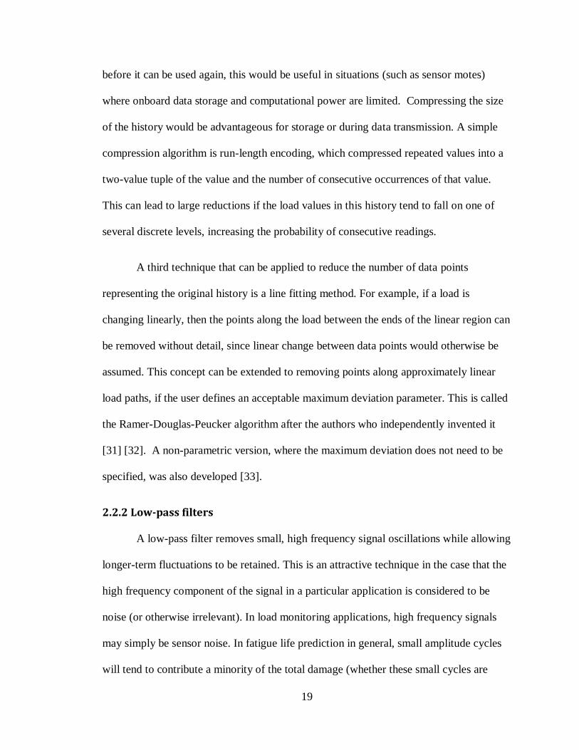
2.2.2 Low-pass filters

A low-pass filter removes small, high frequency signal oscillations while allowing

longer-term fluctuations to be retained. This is an attractive technique in the case that the

high frequency component of the signal in a particular application is considered to be

noise (or otherwise irrelevant). In load monitoring applications, high frequency signals

may simply be sensor noise. In fatigue life prediction in general, small amplitude cycles

will tend to contribute a minority of the total damage (whether these small cycles are

20

generated by noise or if they are actually experienced by the monitored system).

Examples of smoothing filters usable on a time-series load history include moving

average (shown below in Figure 4), lowess, and Savitky-Golay. This technique

contributes to data reduction because less cycles will be extracted during the cycle

counting, decreasing the time required to perform the extraction and shortening the list of

extracted cycles.

Figure 4: Low pass filter on a time-temperature history

Low-pass filters generally require an input parameter, such as the span of a

moving average. This span defines how many data points are within the smoothing

window. Higher spans will lead to more smoothing, at the risk of details being averaged

out of the history. Low-pass filters work best when there is noise that is higher frequency

and smaller in amplitude than the signal. Histories with high sampling rates (relative to

the rate of change of the signal) tend to be better candidates than those with smaller

sampling rates, since the same span will include a larger amount of time. Vichare [29]

explored using a moving average prior to rainflow counting, reasoning that high

frequency noise would be averaged out without impacting the overall history. The span

21

(also called the smoothening parameter or smoothing parameter) was suggested to be the

square root of the sampling frequency (in hertz) rounded to the nearest integer.

A problem with low-pass filters is that they inherently average out the peaks in

the data, making damage estimates less conservative since extracted cyclic ranges are

attenuated.

2.2.3 Range threshold filtering

Range threshold filtering is a data reduction technique which eliminates cycles

below a certain cycle amplitude. Cycles smaller than this are deemed to be irrelevant

(e.g., they are an artifact of signal noise or that they cause a negligible amount of

damage) and are eliminated.

One example of a range threshold filtering technique is “Ordered Overall Range”

the user picks a “reversal elimination index”, S. This represents the ratio to the largest

observed cycle to the threshold amplitude that is to be eliminated. Based on this value,

the time series history is translated upwards S/2 and downward S/2. Beginning at the start

of the time series, a path is drawn to the first peak or valley of either of the higher or

lower offset history (whichever occurs first). Then, the shortest possible path is drawn

through the two offset histories. This forms a path from the beginning of the history to

the end of the history. Whenever this path experiences a local extrema, the corresponding

point in the original history is flagged. Finally, all of the points in the original history

which are not flagged are discarded, successfully eliminating monotonic data as well as

cycles smaller than the threshold. This reduction strategy has been used with rainflow

counting [34], including three-parameter rainflow counting [26] [16]. This reduces the

22

number of points in the original history as well as the number of cycles extracted.

However, since the monotonic data is discarded, all the detail about load path between

extrema is lost.

2.2.4 Damage exponent based reduction

Many fatigue damage models follow a power-law relationship with cycle

amplitude (e.g., Basquin’s law, Coffin-Manson relationship). Consequentially, this causes

higher-amplitude cycles to cause a higher fraction of the total damage during a history

than smaller cycles. This imbalance is more severe as the damage exponent increases. As

a result of this relationship, a damage model with a larger damage exponent can tolerate a

more aggressive small cycle elimination strategy (i.e., setting the range threshold

comparatively higher than if the damage exponent were smaller) while keeping a similar

damage prediction. Vichare [29] suggested that for damage models where the damage is

proportional to the temperature range raised to an exponent, n, the threshold range can be

chosen to be the nth root of the maximum temperature range measured. However, the

trend of this rule is that for higher damage exponents, the threshold value remains more

stable as the maximum observed range increases. This does not match with the

observation that when damage exponents are higher, the larger cycles tend to dominate

the percent of total damage more than for smaller damage exponents. Therefore, the

threshold value should rise more quickly (as a function of increasing maximum range)

when the damage exponent is higher, since more cycles can be removed without

significantly impacting the damage estimation. This strategy also cannot be used in cases

where the damage exponent is a function of cycle parameters. For example, in the

Engelmaier’s model, the exponent is partly a function of mean temperature and dwell

23

time, so there is no exponent to base a threshold on. This technique requires rainflow

counting to have already been performed before data reduction can occur.

2.2.5 Damage estimate reduction-based reduction

Choosing a range threshold prior to cycle extraction does not take into account

cycle frequency. While fatigue damage tends to be dominated by large cycles, in many

cases the smaller cycles are much more frequent. It can occur that even though the

smaller cycles individually contributes a minimal amount of damage to the total, the

frequent occurrence of these cycles make them more important than the larger cycles in

total. If the results of the cycle counting are binned into a histogram, the damage per

cycle can be multiplied by the frequency of that cycle to obtain the damage per cycle

type. With this information, the engineer can choose an acceptable level of damage to

remove when deciding which bins to remove. This technique requires rainflow counting

to have already been performed, as well as the damage estimation per cycle type.

2.2.6 Binning

Instead of storing the results of rainflow counting as a list of cycles, oftentimes

the results are binned into a one dimensional or two dimensional histogram, depending on

how many parameters are extracted (i.e., just the range or both the mean and range). As

the number of parameters extracted during rainflow counting increases (e.g., if dwell is

also extracted in addition to range in mean), the histograms will tend to become more

sparse as a result of the curse of dimensionality. For example, if n cycles are extracted

from a history, and only the range of each cycle is recorded, these ranges can be stored in

a histogram m bins wide. Therefore, the average number of samples per bin is n/m. If the

mean is also binned into a histogram m bins wide, the average number of samples per bin

24

is n/m2. If dwell times are extracted beyond that, the average number of samples per bin

becomes n/m3, and so on. As a result, histograms will become less space efficient as their

dimensionality rises, due to the number of zero-count bins that must be stored, and the

diminishing likelihood that multiple cycles occur in the same bin (i.e., they have similar

enough extracted cycle parameters in each binned dimension to be placed with another

cycle). A more efficient structure in this case would be a sparse array, where a list of

observed bins as well as the observed frequency is recorded, so that bins with no counts

do not take up space.

Bin size can impact the representation of the data. Bins that are too small will lead

to less data reduction, but will also over-represent the random variation in the population.

If the histograms are intended to represent a probability distribution, this situation is

referred to as “undersmoothing.” Conversely, if the bins are too large, too much detail is

lost. This is called “oversmoothing.” Optimal binning rules have been developed to

mitigate this [19] [18].

Chapter 3: New Multi-parameter Rainflow Counting

Prior art versions of rainflow algorithms for extracting temporal parameters (e.g.,

dwell time or cycle period) have several shortcomings. First, current algorithms require

the load history to be simplified into a sequence of peaks and valleys. However, this

makes it impossible to accurately account for how the load varies between consecutive

extrema. This can make a difference when calculating parameters such as dwell time or

ramp rate. A hypothetical load half cycle which features long dwells at either extrema

with a sharp ramp between them should not be treated the same as another half cycle

25

where the load varies linearly between the two extrema. However, if monotonic data is

discarded, the difference between these two load paths is lost.

Current rainflow algorithms also discard cyclic sequence. If it assumed that

damage cannot be summed linearly, this causes a problem. It is possible that material

exhibits a sequential effect in fatigue damage accumulation. Materials can cyclically

harden or soften over the course of their life. This can be accounted for in a non-linear

damage model, where the cycles must be added in the sequence that the damage

occurred. Therefore, if a rainflow counting algorithm records the sequence in which the

cycles occurred in the original time series history, they can be summed non-linearly in

the correct order.

It is also sometimes desirable to generate simplified load histories for testing

purposes. This can be accomplished by applying a rainflow algorithm, discarding cycles

contributing small amounts of damage, and then reconstructing the history based on the

cycle list. If the original starting times of each half cycle was not recorded, this reverse

transformation from the cycle list to a time series history could not be uniquely done. The

engineer would need to choose where to place intermediate cycles onto larger cycles,

rather than using their original time stamp.

Treatment of dwell time in the prior art has been inadequate. Since rainflow

algorithms currently simply the load behavior to sequences of extrema, it is impossible to

make a determination of dwell periods. Current methods, because of the removal of

monotonic data, are forced to assume that dwell times are a fixed fraction of half cycle

time, or they need to determine dwells prior to cycle counting. However, if dwells are

26

counted prior to cycle counting, the dwells are inherently not connected to any particular

cycles. Therefore, this defines dwell differently than a damage model which requires a

dwell for a particular cycle (e.g., Engelmaier’s model), and it therefore not useful for

such a model. It would be advantageous to develop a dwell estimation method which

took load path (i.e., monotonic data within a cycle) into account for each individual cycle

that is extracted.

3.1 Proposed Algorithm

The dwell time is the time an element remains in a given state. For example, in an

idealized load path, it is the time the test specimen remains at a given load level before

ramping up or down. In a more flexible definition, the JEDEC standard for temperature

cycling [35] defines soak time (i.e., dwell time) as a part of the cycle period occurring in

a particular range of the extreme. Specifically, Therefore, it is the time where the load is

within +15°C to -5°C of the maximum sample temperature specified by the profile or

within -15°C to +5°C of the lower temperature specified by the profile. Therefore, since

soak time (analogous to dwell time) is defined in terms of cyclic range, it is reasonable to

calculate dwell time of a cycle based on the amount of time the load dwells within a user-

defined fraction of the cyclic range. A hard number such as 5°C would not generalize

well as maybe times cycles smaller than this range may be extracted. A fixed percentage

could instead be used to define the dwell region, so that the time spent within this region

towards either extreme of the half cycle is defined as dwell time. For example, the top

and bottom 25% of the range can be defined as dwell regions (illustrated in Figure 5), and

the dwell times can be calculated based on that definition. Since the 75% and 25% lines

27

will not necessarily fall on a particular data point, it is necessary to interpolate where the

dwell regions begin and end.

Figure 5: Dwell time definition based on load range percentage

The load range percentage may be chosen in order to make the estimate robust to

small ramp ramps (which the engineer may assume is essentially dwell) or discretization

error (where the load might have dwelled but the true load was not sampled fast enough

to “catch” the flat regions.” Choosing a load range percentage N so that it is resilient to

small slopes first involves choosing a threshold slope (αt ) below which ramps are

insignificant. Choosing a threshold slope of zero classifies only strictly flat regions as

dwell, and a threshold slope of 90 should classify the entire load path as dwell. Therefore,

the following equation may be used:

𝑁 =cos∝𝑡

1.8 (3.11)

In order to make the estimate robust to discretization error, the average number of

half cycles extracted divided by the number of data points in the history should be

calculated in order to find the average number of points per half cycle. If there is only

28

two points per half cycles, there is no load path information between extrema and the

load range percentage N should be assumed to be half of the half cycle time (assuming

that each cycle comprises an equally proportioned ramp up, an upper dwell, a ramp

down, and a lower dwell). As the point density increases, N can be lowered since the

possible discretization error lessens. Therefore, the following equation can be used:

𝑁 =100

4((𝑁𝑝

𝑁𝑐)−1)

(3.12)

The maximum between these two equations can be used as the load range

percentage.

When a cycle is extracted (using a standard extraction criteria [2]), the half cycle

time of the first of the two independently treated half cycles can be simply calculated as

the difference between the two data points in the time dimension. The end of the second

half cycle may need to be interpolated if that does not fall on a data point. If the

beginning or end extreme of a half cycle falls on a “flat peak” (i.e., multiple points at the

same load consecutively), the middle point can be used. Next the load thresholds are

calculated based off the user-chosen range-threshold parameter (e.g., 25%), and the point

where the half cycles cross these thresholds (two thresholds per half cycle) is

interpolated.

Another two parameters which can be extracted are the start times of each half

cycle. This is valuable in order to enable non-linear damage summation, in case each

thermal cycle must be summed in the same order to model load-sequence effects. It also

allows the used to reconstruct the original time-temperature history by mapping the

29

extracted cycle list to locations in time in the original history. A third thing that is

enabled by recording the start times of each half cycle, is the conversion of the damage

vs. number of cycles history typically reported for fatigue damage to a damage vs. time.

Since the half cycle start time and duration is known, and the damage per half cycle can

be calculated, the damage spread out over the cycle duration could be superposed onto a

time series at the correct time to estimate a damage rate vs. time history. This curve can

be integrated to show a cumulative damage vs. time history. This curve can be used

simply for visualization purposed, or to train probabilistic time series models (e.g.,

autoregressive models) to generate probabilistic damage estimates using the time series

rather than sampling probability distributions.

Another option after extracting a cycle, is whether to subtract the cycle period

from the remainder of the time series history. If the cycle period is not removed, the cycle

time would be “double-counted” as occurring during both the extracted cycle and the half

cycle it was extracted from. Enabling “time removal” would assign dwell time to only the

extracted cycle, resulting in a shortened residual half cycle from which the extracted

cycle was taken. This is illustrated below in Figure 6. A range formed by consecutive

extrema interrupts an overall range. The middle plot shows the half cycle formed by the

overall range after extraction in the case that time removal was not performed. The

bottom plot shows the same in the event that time removal is enabled, resulting in a

shorter (in the time dimension) residual half cycle.

30

Figure 6: Time removal illustration

When this time removal is performed during fatigue analysis, it shortens the time-

length of the residual half cycle form which two half cycles are extracted. In the event

that significant time-dependent strains (e.g., creep strains) during the loading or the

unloading of the test specimen, the cyclic stress-strain loop will look different is time

removal is enabled or not. Assuming less time-dependent strain (in the case of enabled

time removal) will make the loop smaller. In fatigue analysis, the fatigue damage is

related to the area formed by the cyclic stress-strain loop. Therefore, enabling time

removal will result in a lower damage prediction. Therefore, for fatigue analysis, time

removal is not recommended since it will result in a less conservative damage prediction.

31

The overall process to perform the algorithm is shown below in the flowchart in

Figure 7. First the time series data is imported. The series is rearranged to start at the

most extreme value. In order to retain the cycle sequence of extracted half cycles, two

time vectors are retained: one monotonically increasing “false time” vector starting at the

minimum time value and one “true time” vector which keeps the original time stamp of

the data point. If on-board memory is an issue, there could just be a function mapping the

false time to the true vectors rather than saving both. This would be generated after the

rearranging of the data to start at the most extreme point. When the time series is

rearranged, the user can choose how much time is elapsed between the two parts to form

one continuous history. The sampling increment can be used for this value, for example.

Appending the two portions together assumes that the load history is periodically

repeating and does not exhibit an upward or downward trend over time.

From this rearranged history, all the load reversals are flagged. This can be done

in a logic mask, where every index (corresponding to the false time vector) at which a

reversal occurs is marked with “true,” and all other points are marked as “false.” When a

reversal falls on a flat peak (i.e., the load dwells on a constant value for consecutive time

indices), the middle index should be selected as the reversal index.

Next, the reversals are evaluated by conventional three-point rainflow cycle

extraction criteria [2], shown below in Figure 8. If a range is smaller or equal to a

preceding range, it is removed from the history. If the algorithm is evaluating the first

point in the history, one half cycle is extracted and all data until the next reversal is

removed. If the first point in the history is not under consideration, the two reversals

under consideration are removed and all points until the end of the second half cycle are

32

also removed (shown in Figure 10). If time removal is enabled, the elapsed time of the

extracted ranges is removed from the remained of the history.

For the first half cycle, the elapsed time is calculated between the two extrema

under consideration. Shown in Figure 9. If the second half cycle is also being extracted,

the end time is interpolated to find the time when the load is again equivalent to the first

reversal. If the end of the second half cycle falls on a flat region, the middle index should

be selected. Next, for each half cycle, the user-input load range threshold, L, is used to

calculate the upper and lower dwell time. The time corresponding to the upper value

minus range*L and the time corresponding the lower value plus range*L is interpolated.

These two times are used to section the total half cycle time between the upper dwell,

ramp time, and lower dwell regions. For each extracted half cycle, the entry from the

“true time” corresponding to the original start time of the half cycle is recorded.

Therefore, a six-entry long row in the output matrix can be formed for each extracted half

cycle: range, mean, first dwell time, ramp time, second dwell time, and start time.

33

Figure 7: Flow chart for the proposed algorithm

34

Figure 8: Detailed flowchart for the half cycle extraction step

35

Figure 9: Detailed flowchart for the dwell time calculation step

36

Figure 10: Detailed flowchart for the data deletion step

In conventional two-parameter rainflow counting, the output results would be

binned into a matrix. However, because of the additional extracted parameters, there is a

disadvantage of binning. First, simply because of the larger number of parameters in

itself, the bins will tend to be sparse (due to the “curse of dimensionality”), reducing the

usefulness of binning at all. Balancing this fact against the possible discretization error in

rounding cycles into bins, an engineer may choose to simply analyze the cycle list

without binning. If binning is performed, a list of bins (with each bin corresponding to a

unique combination of extracted parameter levels) will often be a more efficient storage

structure than a full multidimensional histogram due to the likely sparsity of the array. If

time removal is disabled, there may be extreme values of dwell time in long datasets that

may substantially increase the bin width calculated by existing optimal bin width

formulas, degrading damage predictions. In this case, non-linear bin spacing may prove

37

advantageous. In many cases, dwell times are observed to have a highly skewed

distribution, with much more density towards the low end. However, because some

higher values are observed, the bins will widen to accommodate the full range. This

degrades the resolution of the histogram at the low end (where density is highest) and

potentially causes inaccuracies. Future work to solve this problem may include optimal

binwidth algorithms with non-linear spacing for highly skewed, long-tailed distributions

(such as lognormal).

3.2 Comparison to prior methods

For purposed of comparison, the new algorithm featuring a range-threshold based

dwell definition was run on four different datasets, shown below in Figure 11. They were

also processed using Cluff’s [26] half-cycle time definition of dwell time, and Vichare’s

supplemental [29] algorithm for extracting dwell times.

The first dataset is a thermal cycling test profile used by Chai [36]. This profile is

a periodically repeating temperature pattern recorded in a thermal cycling chamber. The

temperature cycling history consisted of small cycles (having a mean of 65°C and

amplitude of 20°C) superimposed onto the top peaks of larger cycles (having a mean of

25°C and an amplitude of 100°C). The large cycle represents a system being turned on

for the day, and the minicycles represent variations in usage throughout the day. The

temperature sampling period was one minute and the length of the history file is 8,486

minutes. After performing rainflow counting, the half cycle density (the observed half

cycles divided by the total number of data points is 0.11 half cycles per data point. There

are 27 unique values of temperature observed over a range of 100°C. To quantify the

amount of the history that is dwelling at a constant temperature, a “dwell fraction” is

38

calculated by counting the number of data points preceded by a point at the exact same

load, then dividing by the total number of data points. The dwell fraction for this data set

is 0.58. To quantify the amount of nonlinearity between extracted extrema, a “non-

linearity parameter” is calculated by finding the maximum deviation between the load

path and a linear path between the two extrema as a cycle is being extracted, normalized

by the extracted range, summed for every extracted half cycle, and divided by the total

number of half cycles. This parameter is about four times higher for the test dataset than

the next (outdoor) dataset.

A second dataset was recorded from an outdoor telecommunications application.

It is a temperature measurement from a circuit board, rather than the ambient

temperature. This dataset tends to have less consecutive points occurring at the same load

(“flat regions”) and features several high amplitude cycles where the temperature drops

abruptly for several data points. There is a relatively small amount of monotonic data

between reversals as a consequence of the large sampling period compared to the large

swings in temperature. The temperature was sampled every fifteen minutes for 10,050

minutes. The half cycle density is 0.54 half cycles per data point. There are 657 unique

values of temperature spread over a range of 45.6°C. The dwell fraction of this data set is

0.021. This dataset has the smallest non-linearity parameter out of all datasets considered.

A third dataset is from a laptop central processing unit temperature sensor. This

data was sampled at one point per second for 36,668 seconds. This gives it a much higher

sampling rate than the other three datasets. There are 0.47 half cycles per data point.

There are 151 unique values of temperature spread over a range of 19.9°C. The dwell

39

fraction of this data set is 0.20. The non-linearity parameter in this data set is about twice

as high as in the outdoor dataset.

A fourth dataset was recorded on a desktop graphics processing unit temperature

sensor. The temperature was sampled every minute for 19,649 minutes. The observed

half cycle density was 0.28. There were 12 unique temperature values over a range of

17°C. Of the four data sets, this one was the most discretized (e.g., smallest number of

unique values). These datasets are illustrated below in Figure 11. These datasets will be

referred to as “test profile”, “outdoor”, “laptop” and “desktop”, respectively. The dwell

fraction of this data set is 0.70. This is the highest dwell fraction out of the four datasets,

which is likely a consequence of the discretized temperature values. The non-linearity

parameter is about four times as high as in the outdoor data set.

40

Figure 11: Each of the four data sets under consideration

The average dwells, without time removal enabled, are given below in Table 1.

The average dwells are somewhat correlated to the sampling rate, with the outdoor

dataset consistently causing the highest average dwells. This could be a consequence of

41

less small (in range), short (in time) cycles being extracted which could only be picked up

by a high sample rate, such as in the laptop dataset. For the proposed algorithm, a load-

range percentage of 25% was used to define dwell. This was chosen because this would

give the same result as a 50% half cycle time prediction (Cluff’s dwell definition) in the

event that there was no monotonic data between two extrema, or if that monotonic data

was purely linear.

Table 1: Average dwell values

Cluff Vichare Proposed Units

Test

profile 4.5 5.2 7.2 min

Outdoor 55.6 30 62.8 min

Laptop 5.2 1.3 7.8 s

Desktop 6.6 4.9 9.3 min

The normalized average dwell estimations for the outdoor, laptop and desktop

data sets are shown below in Figure 12. In the top figure, for the test profile data set, each

estimate is normalized to the Vichare’s method estimate since it most literally finds flat

regions in a data set where such flat regions occur. In the bottom figure, each bar is

normalized to the prediction shown in the red bar. For the proposed algorithm, the load-

42

range percentage of 25% was again used. For Vichare’s method, the estimate was made

with a 0ºC/s rate threshold and a 0ºC range threshold.

Figure 12: Average normalized dwell times for test profile (top) and the three remaining estimates (bottom)

The damage per half cycle was calculated with Engelmaier’s model using the

material and geometry constants reported by Chai [30]. The total damage was summed

linearly with Miner’s rule. Because the damage is calculated in the same way as Chai, the

results can be compared to those experimental results. Below in Figure 13, the black line

is the experimental results. The recorded history file was approximately ten percent of the

0 0.2 0.4 0.6 0.8 1 1.2 1.4 1.6

Vichare

Cluff

Range-based

Avg. dwell, normalized to Vichare's estimate

0.0

0.2

0.4

0.6

0.8

1.0

Outdoor Laptop Desktop

Norm

. A

vg

. D

wel

l T

ime

Vichare (supplementary)

Cluff

Range-based

43

length of the reported time to 50% failure of the sample population. Therefore, the

damage is shown on the graph below at approximately 0.1 to represent the fraction of life

consumed at the end of the history file.

The blue lines are the damage estimate using Engelmaier’s model, over a range of

load-range percentages (the required input parameter to the proposed method). The solid

blue line was calculated with an F value (the non-ideal factor in the Engelmaier model).

This non-ideal factor is a function of package type. For this particular package type

(leadless), the non-ideal factors are reported to be typically between 0.7 and 1.2 [10].

Therefore, the lower dashed blue line was calculated with an F value of 0.7 and the upper

blue dashed line was calculated with an F value of 1.2. This gives some indication of the

deviation between the experimental result and the estimate is within reason.

Although the estimate seems to improve at high values of load-range percentage,

this single example cannot, by itself, be generalized to support the use of a high load-

range percentage. Using 50% is classifying the entirety of each half cycle as dwell, while

using 0% is not extracting any dwell time at all. This curve was calculated from 1% to

49%.

44

Figure 13: Comparison to experimental data

Next, Table 2 below shows the damage fractions at the end of each history for the

rest of the data sets, using all three dwell definitions. The proposed definition- and the

Cluff definition-based dwell estimations are performed both with and without time

removal.

Table 2: Estimated Damage

Cluff Proposed

Vichare No Removal Removal No Removal Removal

Outdoor 9.0E-03 6.6E-03 3.9E-03 6.8E-03 4.1E-03

Laptop 4.9E-05 8.2E-05 8.5E-07 1.1E-04 9.4E-07

Desktop 1.4E-04 1.2E-04 2.4E-05 1.3E-04 2.4E-05

The next chart, Figure 14, shows the same information normalized to the

proposed result (no time removal performed). Similarly to the results showing the

average dwell times, the Cluff and the proposed methods match closest during the

outdoor dataset since that data exhibits the least amount of monotonic data between

extracted extrema. The Vichare method’s results do not follow a clear trend relative to

the other estimated, which is expected since it does not define dwell as being contained

within a particular cycle, unlike the other two definitions.

Enabling time removal in the laptop dataset decreased the damage prediction,

almost to zero. More than in the other datasets, the extracted cycles left such little dwell

time left in the history for the larger remaining half cycles that they were extracted from

45

so that the time-removal enabled damage estimate was attenuated by orders of

magnitude. While the impact is not quite as large in the other two datasets, it still makes a

40% difference in the outdoor dataset and an 80% difference in the desktop dataset.

Enabling time removal makes the damage prediction much less conservative, in all of

these cases.

Figure 14: Normalized damage estimates

The percent differences between the damage results using the Cluff dwell time definition

and the range-based (proposed) dwell time definition were within five percent both with

and without time removal for the outdoor dataset. For the rest of the datasets, the

predictions diverged. In Table 3 below, it can be seen that the difference in the test profile

predictions, for example, are much higher (24% difference rather than 5%).

Table 3: Damage Comparisons between Cluff and prosed dwell definitions

Damage

Cluff Proposed Diff.

Test Profile 0.064 0.080 24%

0.0

0.2

0.4

0.6

0.8

1.0

1.2

1.4

Outdoor Laptop Desktop

Norm

ali

zed

Dam

age

Dataset

Vichare

Cluff, No Removal

Cluff, Removal

Proposed, No

Removal

Proposed,

Removal

46

Outdoor (time

removal) 0.0039 0.0041 5%

Outdoor (no time

removal) 0.0066 0.0068 2%

3.2.1 Comparison of Dwell Estimates

Since Cluff’s definition of dwell time is a fixed damage fraction, it does not have

a parameter to specify which impacts prediction. Vichare’s supplemental algorithm and

the proposed load-range based definition, however, each require input parameters.

Vichare’s algorithm allows small ranges and slopes to be treated as flat dwell regions.

Therefore, the threshold for each ranges and ramp rates need to be specified in order to

do this simplification. To analyze the sensitivity of the dwell predictions to the choice of

input parameters, the average dwell time was estimated using range thresholds from 0°C

to 10°C and ramp rate thresholds from 0°C/min to 2°C/min. For comparison, the average

dwell estimate using the proposed load-range based dwell definition was also plotted on

the right in Figures 15, 16, 18, and 20 below. The surface on the left graph is linearly

interpolated within data points for the sake of visualization. The range threshold on the

left graph (in °C) for Vichare’s method and the range threshold (in %) on the right graph

are different parameters. The former is the threshold below which all ranges are

considered dwell, the latter is the threshold percentage of the cycle range near each

extrema is defined as dwell within a particular cycle.

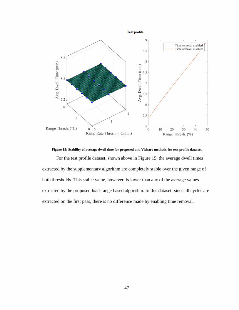
47

Figure 15: Stability of average dwell time for proposed and Vichare methods for test profile data set

For the test profile dataset, shown above in Figure 15, the average dwell times

extracted by the supplementary algorithm are completely stable over the given range of

both thresholds. This stable value, however, is lower than any of the average values

extracted by the proposed load-range based algorithm. In this dataset, since all cycles are

extracted on the first pass, there is no difference made by enabling time removal.

48

Figure 16: Stability of average dwell time for proposed and Vichare methods for outdoor data set

For the outdoor dataset, shown above in Figure 16, the supplementary algorithm

gives a sharp rise in average dwell estimate at higher values of both ramp rate threshold

and range threshold. Since this dataset features a very small amount of monotonic data

due to the coarse sample rate relative to the rapidly changing load, there were few dwell

regions extracted at all without increasing the threshold parameters. Setting both to zero,

only seven dwells were detected. Increasing the ramp rate threshold to 1°C/min, the

number of dwells detected peaked at a range threshold of two before dwells began to

merge together at higher range thresholds, decreasing the number of dwells detected to 28

at a range threshold of 10°C. Increasing the ramp rate threshold to 2°C/min did not alter

the results.

49

The average dwell predictions were also somewhat unstable for the proposed

load-range based algorithm. The average increased as a function of range threshold

percentage to almost 110 minutes, but only to about 25 minutes if time removal is

enabled. Enabling time removal decreased the sensitivity to the average dwell estimates

to the choice in range threshold percentage across all data sets analyzed (except the test

profile, since every half cycle was extracted on the first pass so time removal had no

impact).

Figure 17: Distribution of dwell times for outdoor data set

Looking at the distributions rather than the averages (via a histogram), it is

apparent that while the half-cycle time based definition (Cluff) and the load-range based

definition (proposed algorithm) showed similar-looking distributions, the supplementary

50

algorithm (Vichare) showed a very different pattern. In this case, only a few dwells were

detected in the history using the supplementary algorithm, giving a more discretized

probability distribution compared to the other two. The distributions above in Figure 17

(and Figures 19 and 21 as well) were estimated using 25% load-range percentage for the

proposed algorithm, and 0°C and 0°C/min for the supplementary algorithm. No time

removal was performed. The optimal bin widths were determined using the F-D rule [19].

Figure 18: Stability of average dwell time for proposed and Vichare methods for laptop data set

In the laptop data set shown in Figure 18, the estimated average dwell time surged

as a function of range threshold in the supplementary algorithm. At a range threshold of

0°C, there are 5629 dwell times extracted, but this number decreases to less than 50

across all ramp rate thresholds at a range threshold of 8°C and above. Because this data

set does not have a lot of extreme values (relative to the outdoor set which experiences

51

large maximum ranges), setting the ramp rate threshold so high will classify most of the

history as dwell periods.

For the proposed load-range based algorithm, the average dwell predictions varied

from about 0.01 minutes to about 0.17 minutes. The range of values was again much

smaller when time removal was enabled, making the high end of the range only about

0.035 minutes.

Figure 19: Distribution of dwell times for laptop data set

The distributions of dwells (in Figure 19 above) in the laptop dataset again looked

similar for the time-based estimate and load-range based estimates, but varied most from

the supplementary algorithm. All three distributions are skewed, so that higher densities

are observed towards the lower dwell times.

52

Figure 20: Stability of average dwell time for proposed and Vichare methods for desktop data set

In the desktop dataset, the range of values that the temperature took was fairly

small compared to the range thresholds (for the supplementary algorithm) analyzed in

Figure 20. At the higher end of range thresholds in the supplementary algorithm, almost

the entire history is characterized as a dwell time, leading to average dwell predictions of

over 10,000 minutes. In the proposed load-range based algorithm, the estimated dwells

showed a similar pattern as the outdoor and laptop datasets, where the time removal

decreased the apparent sensitivity of the estimates on range threshold percentage.

53

Figure 21: Distributions of dwell estimates for desktop data set

The distributions (shown in Figure 21) for all three methods look visually similar,

with the supplementary algorithm having a slightly higher density at higher values of

dwell time, and the time-based and load-range based estimates conversely having higher

densities at lower values.

3.2.1 Comparison of Damage Estimates

For each of the data sets, all of the following damage predictions using

Engelmaier’s model (using material and geometry constants from [25]), and Miner’s rule.

For the damage estimates using Vichare’s method (using a supplemental algorithm for

extracting dwell time with 0°C as the range threshold and 0°C/min as the ramp rate

threshold), probabilistic predictions were generated using a Monte Carlo simulation with

54

distributional correlations modelled with Gaussian copulas. For the estimates using the

time-based definition of dwell (Cluff) and the load-range based definition of dwell

(proposed algorithm), deterministic predictions were made using Engelmaier’s model

(with the same constants as before) and Miner’s rule in the same way. The load-range

percentage for the proposed algorithm was set to 25% to match the Cluff method most

closely.

In the outdoor dataset, estimates using Vichare’s algorithm tended to be more

conservative since, on average, higher dwell times were used than in with the other two

methods (shown below in Figure 22). The predictions of the Cluff and proposed methods

matched fairly closely to each other. This is expected, since with the relative lack of

monotonic data in this dataset, the two methods estimated dwell times the same if there is

no monotonic data between extrema. Enabling time removal reduced the damage

estimates by almost 50%. The estimates without time removal fell within the uncertainty

bounds estimated by the Vichare method, but enabling time removal moved the estimates

to the lower extreme.

55

Figure 22: Damage comparisons for outdoor data set

In the laptop dataset, none of the estimates well within the distribution estimated

by the Vichare method (as shown below in Figure 23). The proposed method without

time removal ended up being the most conservative estimate (highest damage prediction),

followed by the Cluff estimate without time removal, and then followed by the Vichare

estimate. Enabling time removal reduced the damage estimates by an order of magnitude,

due to the small cycles being extracted from larger cycles “using up” all of the dwell

time, reducing the impact of the larger ranges.

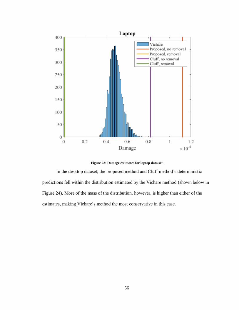
56

Figure 23: Damage estimates for laptop data set

In the desktop dataset, the proposed method and Cluff method’s deterministic

predictions fell within the distribution estimated by the Vichare method (shown below in

Figure 24). More of the mass of the distribution, however, is higher than either of the

estimates, making Vichare’s method the most conservative in this case.

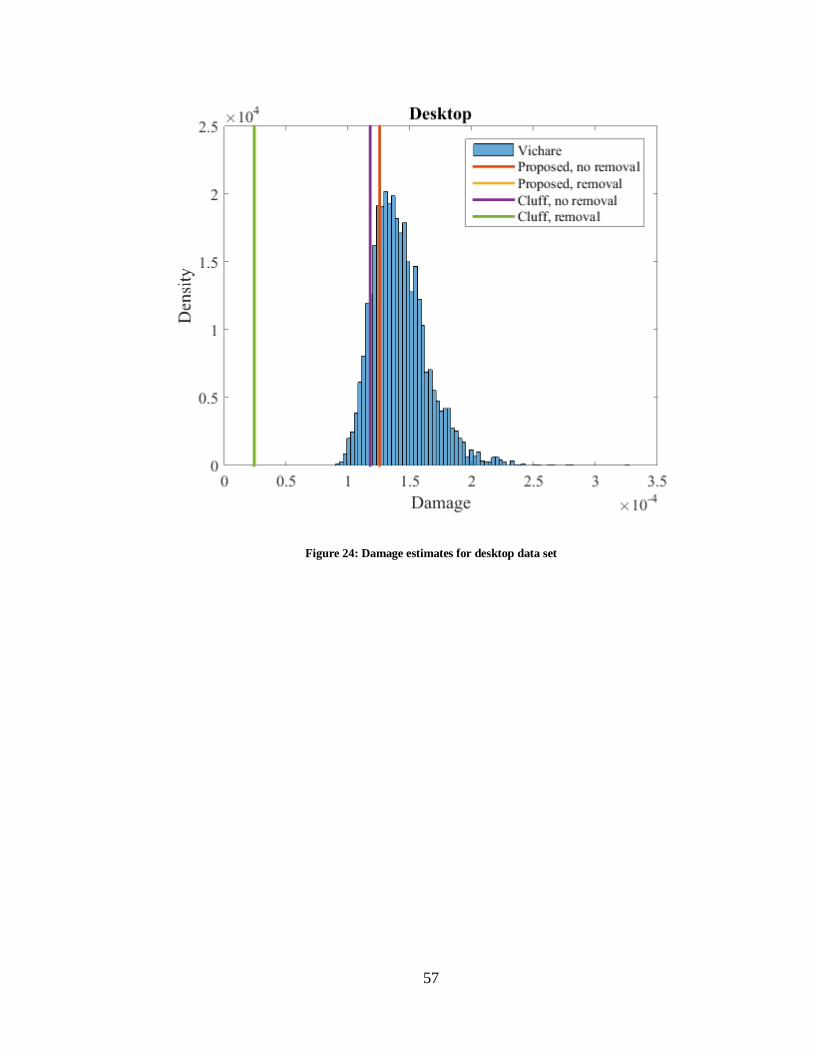
57

Figure 24: Damage estimates for desktop data set

58

3.3 Stability of Damage Estimates in the Proposed Algorithm

Figure 25: Stability of damage estimates for each data set

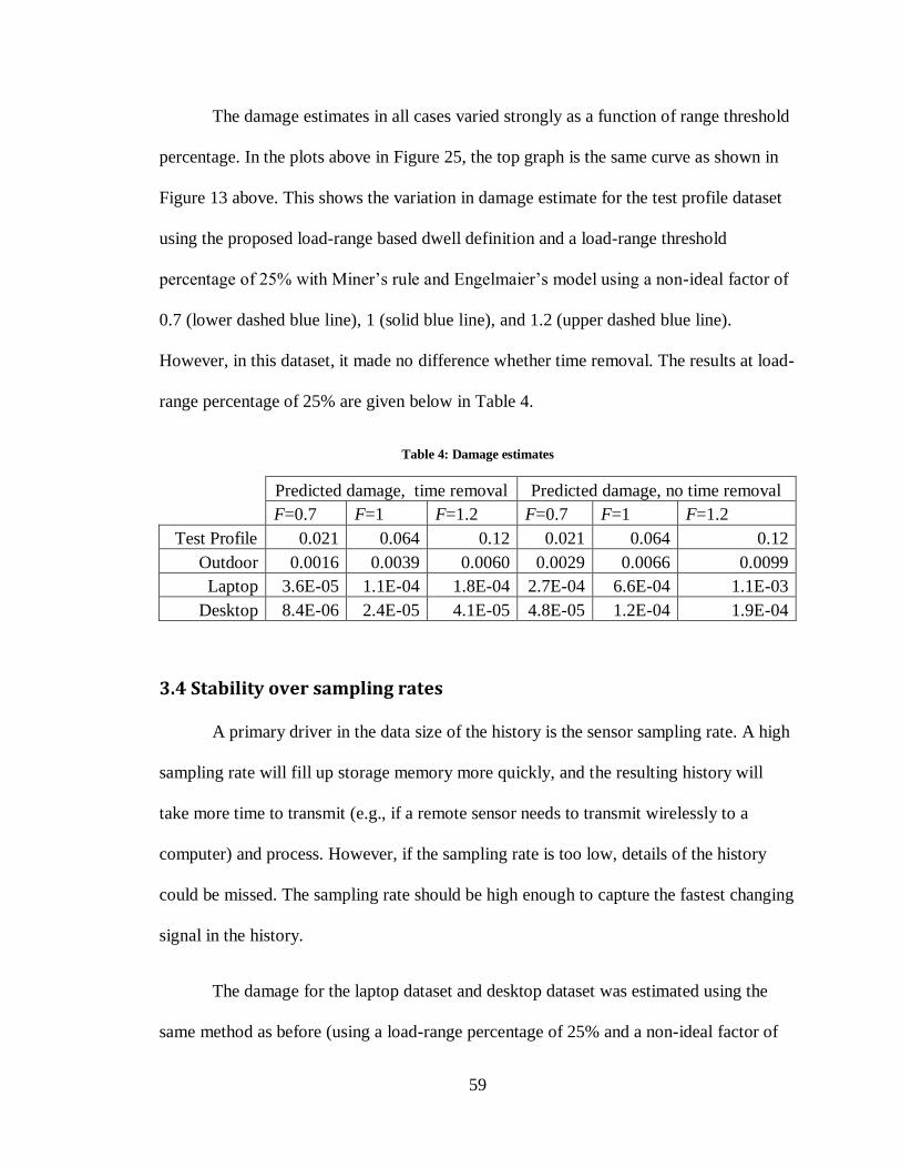
59

The damage estimates in all cases varied strongly as a function of range threshold

percentage. In the plots above in Figure 25, the top graph is the same curve as shown in

Figure 13 above. This shows the variation in damage estimate for the test profile dataset

using the proposed load-range based dwell definition and a load-range threshold

percentage of 25% with Miner’s rule and Engelmaier’s model using a non-ideal factor of

0.7 (lower dashed blue line), 1 (solid blue line), and 1.2 (upper dashed blue line).

However, in this dataset, it made no difference whether time removal. The results at load-

range percentage of 25% are given below in Table 4.

Table 4: Damage estimates

Predicted damage, time removal Predicted damage, no time removal

F=0.7 F=1 F=1.2 F=0.7 F=1 F=1.2

Test Profile 0.021 0.064 0.12 0.021 0.064 0.12

Outdoor 0.0016 0.0039 0.0060 0.0029 0.0066 0.0099

Laptop 3.6E-05 1.1E-04 1.8E-04 2.7E-04 6.6E-04 1.1E-03

Desktop 8.4E-06 2.4E-05 4.1E-05 4.8E-05 1.2E-04 1.9E-04

3.4 Stability over sampling rates

A primary driver in the data size of the history is the sensor sampling rate. A high

sampling rate will fill up storage memory more quickly, and the resulting history will

take more time to transmit (e.g., if a remote sensor needs to transmit wirelessly to a

computer) and process. However, if the sampling rate is too low, details of the history

could be missed. The sampling rate should be high enough to capture the fastest changing

signal in the history.

The damage for the laptop dataset and desktop dataset was estimated using the

same method as before (using a load-range percentage of 25% and a non-ideal factor of

60

1). Then, the damage was recalculated using every other data point. Then it was

recalculated using every 3rd data point, and then every Nth data point. The horizontal axis

on Figure 26 below shows the N value, so at a value of one, every point in the original

time-temperature history was retained. At a value of 60, every 60th point was retained in

the original history to do the damage calculation. No noise filtering was performed on the

original data.

For both histories, there was a general downward trend when time removal was

not enabled. The desktop dataset decayed faster, but the original sample rate of the laptop

dataset was 60 times faster (once per second rather than once for minute). However,

when time removal was enabled, the damage estimates were stable (as a function of N)

relative to the no time removal estimates. However, as expected, the no removal

estimates were consistently higher. This difference decreased as a function of N.

61

Figure 26: Stability of damage estimate over decreasing sampling rates

3.5 Stability over history length

When a long time history is segmented, it breaks up long cycles which would

otherwise span the boundary between segments. This could heavily impact the large

residual cycles left after rainflow counting, which in some case may span almost the

entire original length of this history. However, if time removal is enabled, the residual

cycles will be shorter (in the time dimension) and therefore a smaller sensitivity to history

length is expected.

To explore this, a long time-temperature history was divided into N slices, and the

damage was calculated for each segment. The damage was calculated using the same

62

method as before, with a long-range percentage of 25% and a non-ideal factor of 1. The

damage for all segments in an iteration were summed for comparison’s sake. The plot of

normalized summed damage estimate (relative to the “no removal” unsegmented

estimate) vs. number of segments is shown below in Figure 27. The damage estimate of

the “no removal” version decreased about 20% after 70 segmentations.

While the stability over a range of segments does improve (i.e., the magnitude of

the average rate of change is smaller), the damage estimate still changes. Relative to the

“no removal” unsegmented estimate, the damage estimate increases about 7% after 70

segmentations. Relative to itself (the “removal” unsegmented estimate), the damage

estimate increases about 35%. This analysis implies that, for a stationary load in this

application, a damage estimate based on a small portion of the history will under estimate

damage relative to an estimate on the full history if time removal is not enabled.

Conversely, a small segment may overestimate damage of the full history if time removal

is enabled.

Figure 27: Stability of damage estimates over smaller history lengths

63

3.6 Comparison of Run times and Memory Requirements

Because the new method to estimate dwell time takes into account more details

from the load paths between load reversals, it takes longer to run over a particular history.

The biggest drivers in run time is the number of interpolations required by each. If neither

the end of the second half cycle corresponding to a particular extracted range is not

interpolated, nor the dwells, then the algorithm executes the quickest (out of the options

considered). If the algorithm interpolates the end time of the second half cycle, but does

not interpolate the dwells based on a load range definition of dwell time, the algorithm

slows. It slows further if both the end of the second half cycle and both dwell period for

each half cycle are interpolated.

As shown below in Figure 28, the run times scale approximately linearly with

input history length, although they scale at different rates. Compared to the dwell

interpolation, only performing the period interpolation results in about a 60% reduction in

run time, while interpolating neither results in about a 90% reduction. As shown in Figure

29, there is a slight reduction in memory requirements if the monotonic data is not

considered during extraction. If monotonic data was never saved in the first place, rather

than being deleted by the algorithm itself, the difference between the two lines would be

larger.

64

Figure 28: Run time comparisons

Figure 29: Memory usage comparisons

Chapter 4: Automated Cycle Reduction

When using a damage estimate-based cycle reduction, it is necessary for the user

to choose an acceptable level of damage reduction. An alternative is to use a statistical

test to see if the distribution of observed damage rates during the history has changed

0

50

100

150

200

250

300

350

400

0 20000 40000 60000 80000 100000

Run t

ime

(s)

History Length (pts)

Dwell interpolation

Period Interpolation

No interpolation

0

0.5

1

1.5

2

2.5

3

3.5

4

4.5

5

0 50000 100000 150000

Mem

ory

Usa

ge

(mb)

Original History Length (pts)

Monotonic data retained

Monotonic data dropped

65

before and after reduction, within a particular confidence limit (e.g., 95%). The null

hypothesis would be that the pre-reduction and post-reduction damage rate histories were

from the same distribution.

4.1 Proposed Algorithm

The first step in this process is to calculate the distribution of damage rates. This

can be done by converting the cycle list resulting from rainflow counting, along with the

calculated damage per cycle, into a damage rate vs. time history. This requires that the

half cycle time length and half cycle start time were extracted parameters during cycle

counting. The damage for each half cycle is superposed equally onto the time indices

from the beginning of the half cycle to the end. After superposing all half cycles onto the

history, the damage contained in a particular time index is the damage rate (in units of

time step of the history). If desired, the area under the curve corresponds to the total

damage estimate. The vector of damage rates can be treated as a sample population of a

random variable.

This baseline distribution can be used as a baseline iteratively compare

distributions formed from removing low-damage cycles. After saving the baseline

distribution, the cycle list is sorted in order of increasing damage per cycle. The damage

rate vs. time history is recalculated with the least damaging cycle removed, and the

distribution of damage rates is estimated in the same manner as the baseline distribution.

The two distributions are compared with a statistical test to evaluate the null hypothesis

that the two populations are formed from the same underlying distribution. Since the two

populations are not independent, bootstrapping may improve (i.e., reduce bias of) the

comparison by the statistical test.

66

For the following implementations, the two-sample Kolmogorov-Smirnov test

was used to compare the distributions. This test calculates Kolmogorov-Smirnov statistic,

which is the maximum distance between two empirical distribution functions. As the

number of data points approach infinity, the Kolmogorov-Smirnov statistic will converge

to zero if the two test functions are generated from the same underlying distribution. The

null hypothesis is rejected at a level α between a first sample size n1 and a second sample

size n2 when the Kolmogorov-Smirnov statistic Dα is greater than a critical value, or by

comparing the asymptotic p-value to α. This critical value can be found in a look-up

table, or approximated by a formula assuming large sample sizes:

𝐷𝛼 > 𝑐(𝛼)√𝑛1+𝑛2

𝑛1𝑛2 (4.11)

c(α) is a scaling coefficient. This coefficient can be found in look-up tables or defined by

the inverse of the Kolmogorov distribution at α.

If the null hypothesis that the distributions are from the same distribution is not

rejected, the least damaging cycle is deleted and the statistical test is again performed on

the original baseline sample and the new sample with two missing cycle. This process is

repeated until the null hypothesis is rejected. Since this process can be computationally

expensive based on the length of the history and the number of cycles to delete, this

search may be optimized using a binary search algorithm rather than evaluating cycles in

order.

67

4.2 History Reconstruction

After the list of cycles has been reduced, the original load history can be

approximately reconstructed. Using the information about when the extremes of each

cycle occurred (using the range, mean, half cycle start times and half cycle time lengths),

the points of the original history can be layered onto a history and connected to form a

reduced history. This can be advantageous in condensing a history into a time series

history containing only information relevant to the thermal cycling damage. This could

be useful in planning an irregular load cycling test, so that the life can be simulated

faithfully while minimizing the number of reversals that need to be programmed and

executed. Figure 30 below is a portion of a reconstructed history superposed on top of

the original portion of the outdoor dataset to illustrate the reduction in number of

reversals.

68

Figure 30: Example of reconstructed history for outdoor data set (top) and test profile data set (bottom)

69

4.3 Demonstration of Automated Cycle Reduction and Reconstruction

The automated cycle reduction algorithm was executed on three test datasets (the

test profile dataset did not have enough variation in types of cycles experienced to

appreciably benefit from this cycle reduction) to demonstrate the performance (in terms

of data reduction) of the approach. Each of the plots below (Figures 31-33) shows the

percent reductions in points in the damage estimate (in blue), the number of half cycles

from the cycle list resulting from rainflow counting, and the number of data points in the

temperature history. The monotonic data was not retained in the reconstructed history,

only the reversals. Each of the three reductions are plotted over a range of load range

threshold percentage to evaluate the stability of the data reduction as a function of the

user’s choice in this input parameter.

All three datasets had an extremely small change in damage estimate as a result of

the cycle reduction. This implies that the choice of test is cautious in terms of damage

reduction. However, all three datasets had large reductions in both number of cycles

retained and points in the temperature history. While in the outdoor and desktop datasets,

the cycle lists were approximately cut in half, the laptop dataset experienced close to a

90% reduction in number of half cycles retained. Higher reductions were recorded in the

length of reconstructed histories, but this result is padded by the fact that monotonic data

was not retained.

70

Figure 31: Data reduction for outdoor data set

Figure 32: Data reduction for laptop data set

71

Figure 33: Data reduction for desktop data set

If it were assumed that these datasets extended to be a year a long at the same

sampling rate, and that cycles were extracted at the same rate (extracted cycles per unit

time index of the history) and the reduction in cycles and reconstructed history points

were constant, it could be quantified how much data is saved in a year’s worth of history.

Table 5 assumed that each point in the history features two numbers (time and

load) stored in 8 bytes each, and each half cycle is extracted into 6 parameters (range,

mean, upper dwell, ramp time, lower dwell and start time) in 8 bytes each. While the

savings in terms of megabytes are modest (since all data files were less than a gigabyte to

begin with) in applications where storage space is ample, this technique does allow

sampling rates to be increased substantially to account for fast-changing loads, which

otherwise would have filled a storage medium prohibitively fast. This could be useful

especially combined with a line-fitting data reduction method such as the Ramer-

Douglas-Peucker algorithm to reduce the size of the original time series history.

72

Table 5: Data reduction comparisons

Cycle list History

Original Reduced Original Reconstr.

Outdoor 916 331 561 110 kb

Laptop 716 75 505 25 mb

Desktop 7.09 4.11 8.41 1.37 mb

5. Conclusions

A multi-parameter rainflow algorithm which deletes, rather than retains, monotonic

data between reversals will run faster than if dwell times are interpolated. However, in

datasets where the load frequently varies non-linearly between reversals, the two

approaches to dwell time estimation produce much different damage predictions. In this

case, it may be advantageous to use the slower algorithm that estimates dwell time using

more of the available information.

Using a supplementary algorithm to estimate dwell time is only applicable if the

damage model of choice does not require dwell times to be defined within a particular

extracted cycle. For example, if dwell damage and cyclic damage were calculated as

summed independently, then this approach may be ideal since counting dwell regions and

cycle extraction without interpolating dwells can be implemented in relatively fast

algorithms (compared to cycle extraction with dwell interpolations). However, if dwells

need to be defined for every extracted range, then this approach is unsuitable because it is

definition dwell time improperly. If the counted dwell regions are used to estimate a

probability distribution to be sampled at a one-to-one ratio with ranges and means during

a probabilistic damage simulation, then an unrealistic situation is being simulated, since

73

the dwells have no connection to ranges. The resulting probability distribution would be

artificial as a consequence.

In some mechanisms, such as fatigue, hysteresis loops in stress-strain space need to

intersect, and therefore time removal may be unsuitable. Enabling time removal shrinks

the area of the resulting half-cycles. Since the fatigue damage is related to the area of the

cyclic hysteresis loop, using time removal makes the damage estimate smaller.

If a damage model that can be quickly iterated is available (e.g., does not require an

excessive amount of computational time), damage reduction-based data reduction

strategy can achieve large data reduction percentages. Reductions of about 90% were

observed in some cases without appreciably impacting the damage estimate. The fact that

this process is automated and non-parametric (i.e., does not require the user to specify an

acceptable error tolerance parameter) increases the each of use.

5.1 Contributions

This thesis developed a multi-parameter rainflow counting algorithm to estimate

dwell time using monotonic data and retain cycle timestamps. This allows more of the

available information to be used during damage estimates when dwell time are required

to be defined within a particular extracted cycle, whereas this information was previously

discarded prior to analysis

An automated data reduction algorithm was also developed to remove low-

damage cycles and construct a simplified time-temperature history. Previous strategies

either unacceptable altered the damage estimate of the analysis after reduction, or

74

required the user to choose an acceptable damage level. This method is non-parametric,

so a user does not need to specify such an acceptable error.

5.2 Suggested Future Work

While time removal seems to be disadvantageous based on the large reduction in

damage estimates compared to not using time removal, it would make the analysis result

in more aggressive (i.e. predicting later failures) life predictions. Since it is potentially

such a large change, experimental evidence must be provided in order to justify its use.

Another useful avenue to explore would be the development of optimal binwidth

and bandwidth formulas for non-parametric estimation of highly skewed distributions.

Sample dwell time populations resulting from rainflow counting tended to have higher

densities at lower values. Existing optimal binwidth formulas distorted probabilistic

damage estimates as a result of over-coarsening the bins at low values, where most of the

density lies. In other words, too much deference is given to high extremes and too little is

given to small values. A non-linear binning rule may solve this.

75

Works Cited

[1] N. E. Dowling, "Fatigue in materials: introduction and stress-based approach," in

Mechanical Behavior of Materials, Upper Saddle River, NJ, Pearson Prenctice

Hall, 2007, pp. 446-447.

[2] ASTM International, "ASTM E1049-85: Standard Practices for Cycle Counting in

Fatigue Practices," West Conshohocken, 2011.

[3] C. Amzallag, J. Gerey, J. Robert and J. Bahuaud, "Standardization of the rainflow

counting method for fatigue analysis," International Journal of Fatigue, vol. 16, no.

4, pp. 287-293, 1993.

[4] C. McInnes and P. Meehan, "Equivalance of four-point and three-point rainflow

cycle counting algorithms," International Journal of Fatigue, vol. 30, no. 3, pp.

547-559, 2008.

[5] S. Downing and D. Socie, "Simple rainflow counting algorithms," International

Journal of Fatigue, vol. 4, no. 1, pp. 31-40, 1982.

[6] G. Glinka and J. Kam, "Rainflow counting algorithm for very long stress histories,"

International Journal of Fatigue, vol. 9, no. 4, pp. 223-228, 1987.

[7] IPC, "IPC-SM-785: Guidelines for Accelerated Reliability Testing of Surface

Mount Solder Attachments," Northbrook, 1992.

76

[8] W. Engelmaier, "Fatigue of leadless chip carrier solder joints during power

cycling," IEEE Transactions on Components, Hybrids, and Manufacturing

Technology, vol. 6, no. 3, pp. 232-237, September 1983.

[9] IPC, Design Guidelines for Reliabile Surface Mount Technology Printed Board

Assemblies, Northbrook, Ilinois: IPC, 1996.

[10] W. Engelmaier, "Soldering and mounting technology: performance considerations,"

in Electronic materials handbook: packaging, vol. 1, Materials Park, Ohio: ASM

International, 1989.

[11] W. Engelmaier and A. I. Attarwala, "Surface-mount Attachment Reliability of Clip-

leaded Ceramic Chip Carriers on FR-4 Circuit Boards," IEEE Transactions on

Components, Hybrids Manufacturing Technology, vol. 12, no. 2, p. 284, 1989.

[12] W. Engelmaier, "Solder Joints in Electronics: Design for Reliability," in TMS

Annual Meeting Design of Reliable Solders & Solder Interconnections, 1997.

[13] W. Engelmaier, "The Use Environments of Electronic Assemblies and Their Impact

of Surface Mount Solder Attachment Reliability," IEEE Transactions on

Component Hybrids Manufacturing Technology, vol. 13, no. 4, pp. 903-908, 1990.

[14] J. W. Evans, J. Y. Evans, A. Ghaffarian, K. Lee and C. Shin, "Simulation of Fatigue

Distributions for Ball Grid Arrays by the Monte Carlo Method," Microelectronics

Reliability, vol. 40, pp. 1147-1155, 2000.

77

[15] H. Wei and K. Wang, "A probabilistic approach to predict thermal fatigue life for

ball grid array solder joints," Journal of Electronic Materials, pp. 2314-2319, 2011.

[16] N. Vichare, P. Rodgers and M. Pecht, "Methods for Binning and Density

Estimation of Load Parameters for Prognistics and Health Management,"

International Journal of Performability Engineering, pp. 149-161, 2006.

[17] M. Jones, "Simple boundary correction for kernel density estimation," Statistics and

Computing, vol. 3, no. 3, pp. 135-146, 1993.

[18] D. Scott, "On Optimal and Data Based Histograms," Biometrika, pp. 605-610,

1979.

[19] D. P. Freedman and P. Diaconis, "On Maximum Deviation Between the Histogram

and Underlying Density," Zeitshrift fur Wahrscheinlichkeitstheorie und verwandte

Gebiete, 58, pp. 139-167, 1981.

[20] D. Vose, Quantitative risk analysis, Chichester, NY: Wiley, 1996.

[21] R. Iman and W. J. Conover, "A Distribution-free approach to inducing rank

correlation among input variables," Communications in Statistics-simulation and

Computation, pp. 311-334, 1982.

[22] A. Der Kiureghian and P. Liu, "Structural reliability under incomplete probability

information," Journal of Engineering Mechanics, vol. 112, no. 1, pp. 85-104, 1986.

78

[23] R. T. Clemen and T. Reilly, "Correlations and copulas for decision and risk

analysis," Management Science, pp. 208-224, 1999.

[24] G. R. MacKenzie, Approximately maximum-entropy multivariate distributions with

specified marginals and pairwise correlations, Ph.D. Dissertation, University of

Oregon, 1994.

[25] F. Chai, "Solder Interconnect Life Prediction Under Complex Temperature Cycling

With Varying Mean and Amplitude," University of Maryland, College Park, 2013.

[26] K. D. Cluff, D. Robbins, T. Edwards and B. Barker, "Characterizing the

commercial avionics thermal environment for field reliability assessment," Journal

of the Institute of Environmental Sciences, vol. 40, no. 4, pp. 22-28, July 1997.

[27] M. Denk and M. Bakran, "Comparison of counting algorithms and empirical

lifetime models to analyze the load-profiles of IGBT power module in a hybrid

car," in Electric Drives Production Conference (EDPC), 2013 3rd International ,

Nuremberg, 2013.

[28] M. Nagode and M. Hack, "An online algorithm for temperature influenced fatigue

life estimation: stress-life approach," International Journal of Fatigue, vol. 26, no.

2, pp. 163-171, February 2004.

[29] N. Vichare, "Prognostics and health management of electronics by utilizing

environmental and usage loads," 2006.

79

[30] F. Chai, M. Osterman and M. Pecht, "Strain-Range-Based Solder Life Predictions

Under Temeprature Cycling With Varying Amplitude and Mean," IEEE

Transactions on Device and MAterials Reliability, vol. 14, no. 1, pp. 351-357,

2014.

[31] D. H. Douglas and T. K. Peucker, "Algorightms for the reduction of the number of

points required to represent a digitized line or its caricature," Cartographica: The

International Journal for Geographic Information and Geovisualization, vol. 10,

no. 2, pp. 112-122, 1973.

[32] U. Ramer., "An iterative procedure for the polygonal approximation of plane

curves," Computer Graphics and Image Processing, vol. 1, no. 3, pp. 244-256,

1972.

[33] D. K. Prasad, S. Cho and M. Leung, "A parameter independent line fitting method,"

in The First Asian Conference on Pattern Recognition, Beijing, 2011.

[34] H. Fuchs, D. Nelson, M. Burke and T. Toomay, "Shortcuts in Cumulative Damage

Analysis," SAE Technical Paper 730565, New York, 1973.

[35] JEDEC, "Temeprature Cycling," JEDEC Solid State Technology Association,

Arlington, 2014.

[36] F. Chai, "Solder interconnect life prediction under complex temperature cycling

with varying mean and amplitude," College Park, 2013.

80

[37] W. Engelmaier, "Fatigue of Leadless Chip Carrier Solder Joints During Power

Cycling," IEEE Transactions on Components, Hybrids, and Manufacturing

Technology, vol. CHMT-6, no. 3, pp. 232-237, 1983.

[38] P. P. Milella, "Damage Progression and Accumulation," in Fatigue and Corrosion

in Metals, New York, Springer, 2013, p. 421.

[39] H. J. Grover, Fatigue of Aircraft Structures, Naval Air Systems Command, 1966.

[40] S. S. Manson, A. J. Nachtigall and J. C. Freche, ASTM STP 415: Fatigue Crack

Propagation, Philadelphia: American Society for Testing and Materials, 1967.

[41] ASTM International, "ASTM E1049-85: Standard practices for cycle counting in

fatigue practices," West Conshohocken, 2011.