Multiaxis Rainflow Fatigue Methods for Nonstationary Vibration

T Irvine

Dynamic Concepts, Inc., Huntsville, Alabama, USA

Email: tirvine@dynamic-concepts.com

Abstract. Mechanical structures and components may be subjected to cyclical loading

conditions, including sine and random vibration. Such systems must be designed and

tested according. Rainflow cycle counting is the standard method for reducing a stress

time history to a table of amplitude-cycle pairings prior to the Palmgren-Miner

cumulative damage calculation. The damage calculation is straightforward for

sinusoidal stress but very complicated for random stress, particularly for nonstationary

vibration. This paper evaluates candidate methods and makes a recommendation for

further study of a hybrid technique.

1. Introduction

Endo & Matsuishi (1968) developed the rainflow counting method by relating stress reversal cycles to

streams of rainwater flowing down a Pagoda, in Reference 1 with detailed equations given in Reference

2. Similar frequency domain methods have also been developed but assume a stationary time history,

per Reference 3. Furthermore, rainflow cycle counting has been traditionally used for uniaxial stress

response. The method has been extended to multi-axis responses by defining an equivalent uniaxial

stress via the von Mises, Tresca, or similar combination stress formula. These equivalent methods have

been intended mostly for stationary Gaussian random vibration environments, especially when the

calculations are done in the frequency domain. A multiaxis fatigue method which can be performed in

either the frequency or time domain is the hypersphere method by Pitoiset, Preumont, and Kernilis in

Reference 4. The purpose of this paper is to extend the hypersphere method for use

with nonstationary, non-Gaussian random vibration. The motivation is launch vehicles, which have

inherently nonstationary vibration during their liftoff and ascent phases. But the methodology may be

applied to other vibrating structures as well. A plate undergoing in-plane stress vibration is used as a

numerical experiment example in this paper. The conclusion will propose a hybrid method pending

further research and testing.

2. Fatigue Calculation Challenges

Vibration fatigue calculations are “ballpark” calculations given uncertainties in S-N curves, stress

concentration factors, mean stress, non-linearity, temperature and other variables. Furthermore, the

order of loading over a system’s lifetime may affect the true fatigue life. Note that the Palmgren-Miner

summation assumes that the damage mechanism is the same at higher stress levels as at lower ones.

Perhaps the best that can be expected is to calculate the accumulated fatigue to the correct “order-of-

magnitude.” A particular concern for multiaxis fatigue is that the S-N curve for normal stress may

differ from that for shear stress. Another concern is that the stress response may have principal

directions which change during the loading. This “non-proportional loading” occurs in systems where

the applied loads and stress tensor responses are out-of-phase or at different frequencies.

https://ntrs.nasa.gov/search.jsp?R=20160010330 2018-05-29T14:12:22+00:00Z

3. Candidate Stress Metrics

Again, the intermediate goal is to estimate an equivalent uniaxial stress for a multiaxis stress field.

There are several techniques in addition to the hypersphere method. The von Mises criterion is also

known as the maximum octahedral shearing stress theory and as the maximum distortion strain energy

criterion. The von Mises stress reduces a complex multi-dimension stress field into a single scalar

number which can then be compared to the yield limit for ductile materials. The Tresca maximum shear

stress criterion requires the principal stresses and their differences to be less than the yield stress limit.

Neither the von Mises nor the Tresca method can directly be used for rainflow fatigue calculations

because each gives a rectified stress time history which is always greater than or equal to zero. The

rainflow algorithm requires oscillating stress of both positive and negative polarities with respect to a

zero baseline or other mean value. The workaround is to apply a time-varying polarity scale factor.

4. Plane Stress

Figure 1. Plane Stress Diagram and Transformation to Principal Coordinates

The normal and shears stresses are on shown in the left image. The principal

stresses are on the right.

The example in this paper is based on the plane stress model in Figure 1. The stress tensor for plane

stress is

yxy

xyx (1)

The following transformations are used to convert displacement into strains and stresses at a given

point, per Reference 5. First the strain terms are calculated from the displacements u and v in the X and

Y-axes, respectively.

x

v

y

u,

y

v,

x

uxyyx

(2)

O

O

p

The strains x and y correspond to the X and Y-axes, respectively. The term xy is the

“engineering” shear strain. The stress is then calculated from the strain.

xy

y

x

2

xy

y

x

2

100

01

01

1

E (3)

where

E = Elastic Modulus

= Poisson ratio

The principal stress values and axes are calculated via the eigenvalues and eigenvectors of the stress

tensor. The eigenvalues and vectors allow for a coordinate transformation rotation of the stress tensor

such that the resulting principal stress tensor has zero shear stress, as shown in Figure 1. The equivalent

uniaxial unsigned stresses for plane stress can be calculated from the principal stress components in the

following equations, as taken from Reference 6. Note that each stress term varies with time. The

maximum principal stress p is

21abs(maxp (4)

The von Mises stress vm is

2`221

21̀vm (5)

The Tresca stress tres is twice the maximum shear stress max as

2max2

21tres

(6)

The maximum principal, von Mises and Tresca stress time histories can each be rendered as signed by

multiplying by the following scale factor P. Let P be the polarity, either 1 or -1.

maxmaxP (7)

where max is maximum absolute principal stress

Thus, the signed maximum principal, von Mises and Tresca stresses can be used for multiaxis fatigue

analysis. Note that both the von Mises and Tresca stresses can be calculated from the principal stresses.

There are other candidate methods, including Dang Van, Manson-McKnight, Crossland and critical

plane, which are not covered in this paper. In practice, the accuracy of these methods depends on the

biaxiality ratio, which is the ratio of the minimum and maximum principal stresses at a location on the

surface of a component, per Reference 6. But note that the biaxiality ratio can vary with time, as shown

in the example in this paper. An evaluation of the accuracy of von Mises and the other methods as

compared to test data is given Reference 8. This reference includes a discussion on non-proportional

loading, changing principal stress levels and axes, etc.

5. Hypersphere

The hypersphere method from Reference 4 seeks an equivalent uniaxial stress time history )t(Yc of

the form

n

1i

iic )t(Yc)t(Y (8)

The number of stress components is n, typically 3 or 6, for the cases of 2D and 3D stress fields

respectively. The stress time history for each normal or shear component is )t(Yi . The coefficients

ic are normalized as follows

n

1i

2i 1c (9)

The coefficients are chosen by trial-and-error to maximize the rainflow fatigue damage rate, which is a

time-intensive process relative to the other candidate methods. The equivalent uniaxial stress hyper

for 2D plane stress is

)t(c)t(c)t(c)t( xy3y2x1hyper (10)

5. Fatigue Damage

A rainflow cycle count is then performed on the uniaxial time history per References 1 and 2. The

rainflow results are fed into the cumulative damage calculation. A simple Basquin approach is used for

this calculation in this paper assuming a straight S-N line in log-log format with no endurance limit.

This simplified approach allows for a Palmgren-Miner damage accumulation via Equation (11).

Binning of the stress levels is not required. Failure occurs when the damage reaches or exceeds one

per classical theory, but this threshold may vary in practice. In addition, design standards may apply a

safety margin resulting in a lower threshold. The damage rate is then equal to the accumulated damage

divided by duration, where the cumulative damage index D is

bi

m

1i

i SnA

1D

(11)

where

A = Fatigue strength coefficient

b = Fatigue exponent

m = Total number of rainflow cycles

n = Cycles per stress reversal, either 0.5 or 1 per the rainflow algorithm

S = Stress level for corresponding half or full cycle

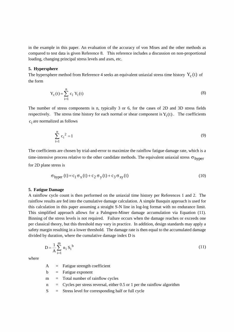
6. Plane Stress Numerical Example

A simple, thin plate, plane stress example is used to compare the hypersphere method with respect to

the other candidates in terms of damage rate. The method was carried out using Matlab scripts. First

a plane stress finite element model was constructed using rectangular Q4 elements, with four nodes per

element and two in-plane displacement degrees-of-freedom per node, per Reference 9. The Q4

interpolation function is bilinear. Hence the displacement and stress values vary across the element.

The stress value for each element is calculated at the element CG for simplification in this example.

The rectangular plate was steel with a respective length, width and thickness of (24 x 23.5 x 0.125

inches), or (61 x 60 x 0.32 cm). The perimeter was fixed for each displacement direction. The

amplification factor was set at Q=20 for all modes. The natural frequencies and mode shapes were

calculated for the model, as shown in Figure 2.

Figure 2. Finite Element Model and First Three Mode Shapes

The unscaled, in-plane displacement field is shown for the modes of interest.

X (in) X (in)

X (in) X (in)

Y

(in)

Y

(in)

Y

(in)

Y

(in)

Undeformed Model Mode 1 fn = 5061 Hz

Mode 2 fn = 5110 Hz Mode 3 fn = 6071 Hz

The model has 625 Nodes, 576 Elements, and 1250 unconstrained degrees-of-freedom. The black circle

in the undeformed plot indicates the node at which separate forcing functions were applied in the X and

Y-axes. Again, the outer perimeter was fixed for the displacements in both the X and Y-axes.

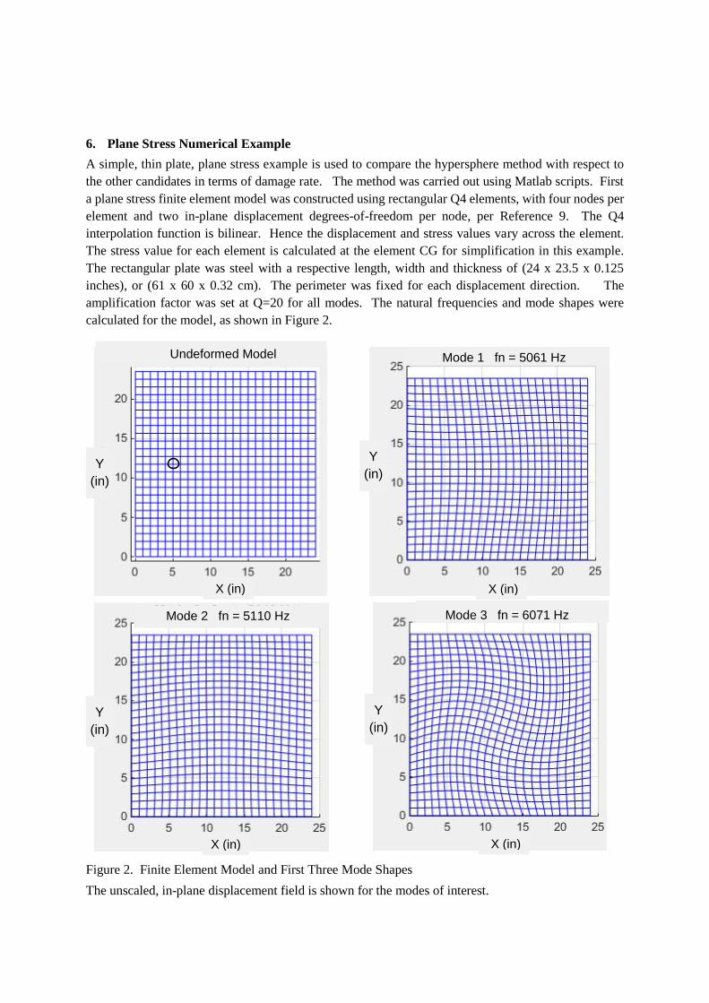
The forcing function for each axis is shown in Figure 3 with a corresponding scatter plot in Figure

4. The functions consisted of sine tones matching the first three modal frequencies as well as random

white noise with amplitude modulations. The white noise was band-limited to a frequency between the

third and fourth modal frequencies. The displacement responses were calculated in the time domain

using the modal transient, digital recursive filtering relationship in Reference 11.

The strain for each element CG was calculated using the corner displacements via continuum

mechanics equations as modified for the Q4 finite element. The stress was then calculated from the

strain. This resulted in two normal and one shear stress time history for each element CG. The three

components were reduced to an equivalent uniaxial time history using the maximum absolute principal,

von Mises, Tresca and hypersphere methods. The uniaxial time histories were then fed into the rainflow

calculation for each method and for each element. Again, the hypersphere method required multiple

trial-and-error iterations to choose the coefficient set which maximized the damage rate. Furthermore,

the hypersphere coefficients varied per element.

Figure 3. Force Time Histories

The sample rate is 72,849 Hz, which is twelve times the third modal frequency.

-2000

-1000

0

1000

2000

0 1 2 3 4

Time (sec)

Forc

e (

lbf)

-2000

-1000

0

1000

2000

0 1 2 3 4

Time (sec)

Forc

e (

lbf)

Force X-axis

Force Y-axis

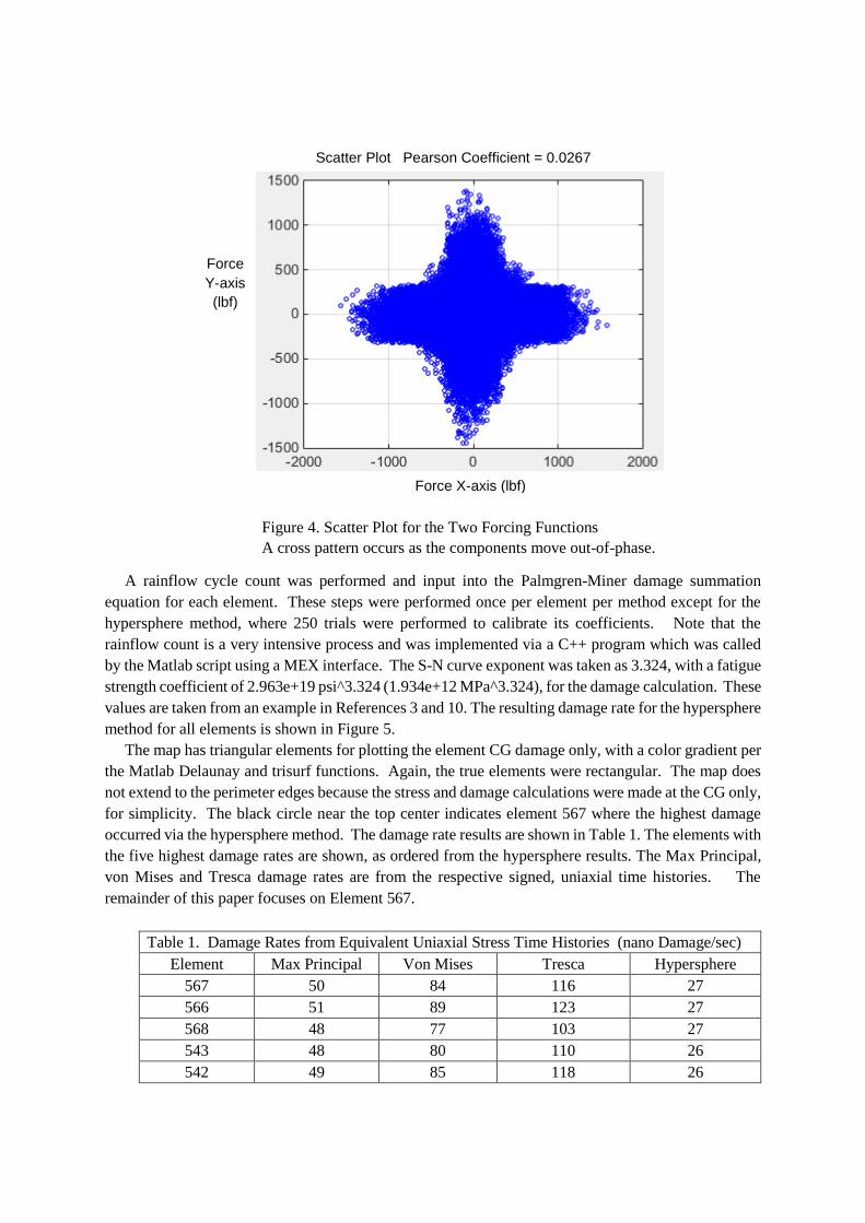
Figure 4. Scatter Plot for the Two Forcing Functions

A cross pattern occurs as the components move out-of-phase.

A rainflow cycle count was performed and input into the Palmgren-Miner damage summation

equation for each element. These steps were performed once per element per method except for the

hypersphere method, where 250 trials were performed to calibrate its coefficients. Note that the

rainflow count is a very intensive process and was implemented via a C++ program which was called

by the Matlab script using a MEX interface. The S-N curve exponent was taken as 3.324, with a fatigue

strength coefficient of 2.963e+19 psi^3.324 (1.934e+12 MPa^3.324), for the damage calculation. These

values are taken from an example in References 3 and 10. The resulting damage rate for the hypersphere

method for all elements is shown in Figure 5.

The map has triangular elements for plotting the element CG damage only, with a color gradient per

the Matlab Delaunay and trisurf functions. Again, the true elements were rectangular. The map does

not extend to the perimeter edges because the stress and damage calculations were made at the CG only,

for simplicity. The black circle near the top center indicates element 567 where the highest damage

occurred via the hypersphere method. The damage rate results are shown in Table 1. The elements with

the five highest damage rates are shown, as ordered from the hypersphere results. The Max Principal,

von Mises and Tresca damage rates are from the respective signed, uniaxial time histories. The

remainder of this paper focuses on Element 567.

Table 1. Damage Rates from Equivalent Uniaxial Stress Time Histories (nano Damage/sec)

Element Max Principal Von Mises Tresca Hypersphere

567 50 84 116 27

566 51 89 123 27

568 48 77 103 27

543 48 80 110 26

542 49 85 118 26

Scatter Plot Pearson Coefficient = 0.0267

Force X-axis (lbf)

Force

Y-axis

(lbf)

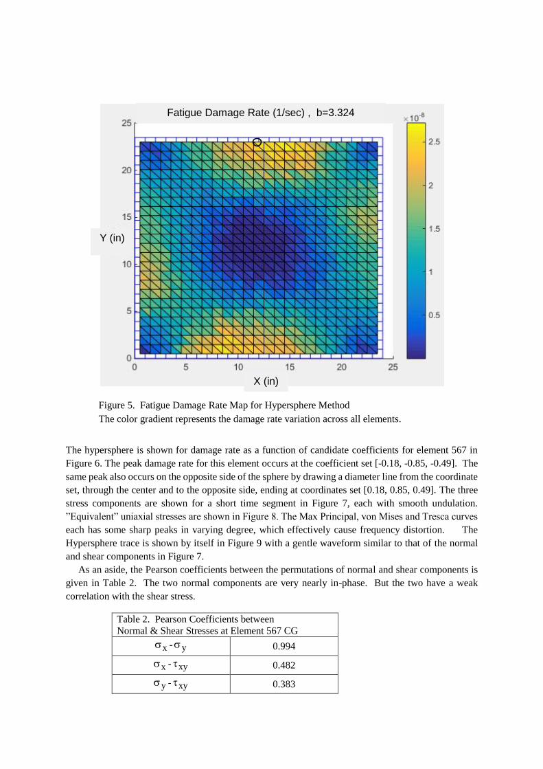
Figure 5. Fatigue Damage Rate Map for Hypersphere Method

The color gradient represents the damage rate variation across all elements.

The hypersphere is shown for damage rate as a function of candidate coefficients for element 567 in

Figure 6. The peak damage rate for this element occurs at the coefficient set [-0.18, -0.85, -0.49]. The

same peak also occurs on the opposite side of the sphere by drawing a diameter line from the coordinate

set, through the center and to the opposite side, ending at coordinates set [0.18, 0.85, 0.49]. The three

stress components are shown for a short time segment in Figure 7, each with smooth undulation.

”Equivalent” uniaxial stresses are shown in Figure 8. The Max Principal, von Mises and Tresca curves

each has some sharp peaks in varying degree, which effectively cause frequency distortion. The

Hypersphere trace is shown by itself in Figure 9 with a gentle waveform similar to that of the normal

and shear components in Figure 7.

As an aside, the Pearson coefficients between the permutations of normal and shear components is

given in Table 2. The two normal components are very nearly in-phase. But the two have a weak

correlation with the shear stress.

Table 2. Pearson Coefficients between

Normal & Shear Stresses at Element 567 CG

x - y 0.994

x - xy 0.482

y - xy 0.383

Fatigue Damage Rate (1/sec) , b=3.324

X (in)

Y (in)

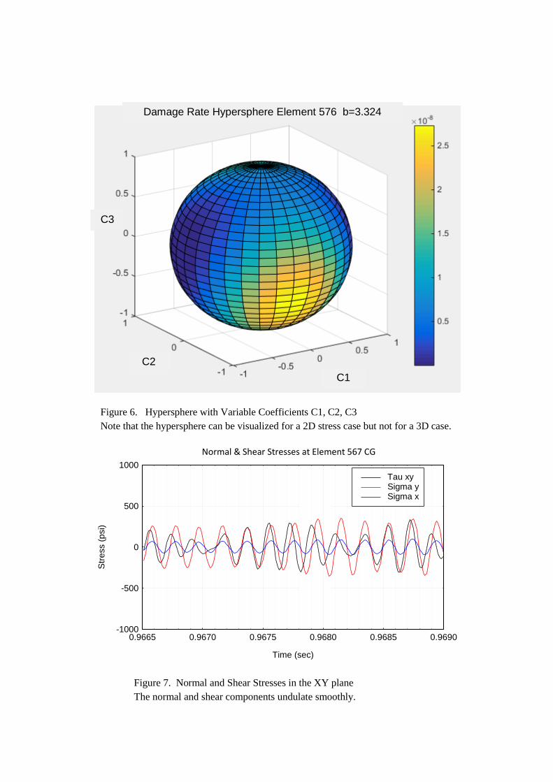
Figure 6. Hypersphere with Variable Coefficients C1, C2, C3

Note that the hypersphere can be visualized for a 2D stress case but not for a 3D case.

Figure 7. Normal and Shear Stresses in the XY plane

The normal and shear components undulate smoothly.

-1000

-500

0

500

1000

0.9665 0.9670 0.9675 0.9680 0.9685 0.9690

Tau xySigma ySigma x

Time (sec)

Str

ess (

psi)

Normal & Shear Stresses at Element 567 CG

Damage Rate Hypersphere Element 576 b=3.324

C1

C2

C3

Normal & Shear Stresses at Element 567 CG

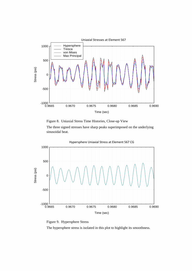
Figure 8. Uniaxial Stress Time Histories, Close-up View

The three signed stresses have sharp peaks superimposed on the underlying

sinusoidal beat.

Figure 9. Hypersphere Stress

The hypersphere stress is isolated in this plot to highlight its smoothness.

-1000

-500

0

500

1000

0.9665 0.9670 0.9675 0.9680 0.9685 0.9690

HypersphereTrescavon MisesMax Principal

Time (sec)

Str

ess (

psi)

Uniaxial Stresses at Element 567 CG

-1000

-500

0

500

1000

0.9665 0.9670 0.9675 0.9680 0.9685 0.9690

Time (sec)

Str

ess (

psi)

Hypersphere Uniaxial Stresses at Element 567 CGHypersphere Uniaxial Stress at Element 567 CG

Uniaxial Stresses at Element 567

CG

The spurious high frequency components in Figure 8 would then appear in the Fourier transforms for

the three signed methods. The rainflow cycle count would be compromised and likewise the

cumulative damage index.

The three signed methods enable relatively fast rainflow and damage calculations, and each is

grounded in a stress theory via principal stresses. The disadvantage is that each represents an effective

rectification and inversion, with the net result being questionable frequency distortion in the respective

uniaxial stress time histories. Furthermore, the Max Principal and von Mises methods may

underestimate the fatigue damage depending on the biaxiality ratio per Reference 7. In contrast, the

Tresca method always yields results which range from adequate to very conservative, again depending

on the biaxiality ratio.

The hypersphere method yields a self-polarized, uniaxial stress time history with no frequency

distortion. But the coefficient calibration is time consuming, and the method lacks reference to any

principal stress based theory. The coefficient calibration must be performed for each element of

interest. The resulting damage index may well underestimate the true damage.

An eclectic hybrid method is thus proposed. The hybrid method begins with the hypersphere’s

uniaxial stress, calibrated for the maximum damage rate. Next, a scale factor is applied to the uniaxial

stress time history prior to the rainflow count and damage calculation. There are two candidate

amplitude scale factors, based on the von Mises and Tresca standard deviation stresses relative to that

of the hypersphere. Note that the standard deviation is the same as the RMS value for zero mean.

Furthermore, the standard deviation is a single value for each method’s time history. The scale factors

in a Matlab-like syntax are

Scale factor 1 = std (von Mises) / std (hypersphere) (12)

Scale factor 2 = std (Tresca) / std (hypersphere) (13)

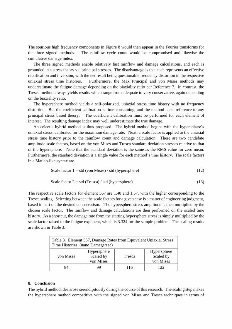
The respective scale factors for element 567 are 1.48 and 1.57, with the higher corresponding to the

Tresca scaling. Selecting between the scale factors for a given case is a matter of engineering judgment,

based in part on the desired conservatism. The hypersphere stress amplitude is then multiplied by the

chosen scale factor. The rainflow and damage calculations are then performed on the scaled time

history. As a shortcut, the damage rate from the starting hypersphere stress is simply multiplied by the

scale factor raised to the fatigue exponent, which is 3.324 for the sample problem. The scaling results

are shown in Table 3.

Table 3. Element 567, Damage Rates from Equivalent Uniaxial Stress

Time Histories (nano Damage/sec)

von Mises

Hypersphere

Scaled by

von Mises

Tresca

Hypersphere

Scaled by

von Mises

84 99 116 122

8. Conclusion

The hybrid method idea arose serendipitously during the course of this research. The scaling step makes

the hypersphere method competitive with the signed von Mises and Tresca techniques in terms of

conservatism, with the advantage of maintaining the pristine frequency content of the normal and shear

stresses. The hybrid method also connects the fatigue damage with existing stress theory via the scaling

process. A potential drawback of this approach is that it feeds some of the von Mises and Tresca

amplitude error into the hybrid stress time history, but the hybrid result still maintains frequency purity

which is vital to the rainflow count.

Alas, this paper’s damage results (from a single plane stress case with a lone pair of orthogonal

nonstationary forcing functions as applied to a common node) are far too tenuous for a paradigm shift

in industrial multiaxis fatigue calculation. Further development of the hybrid methodology would

make a respectable engineering student thesis or dissertation project, especially if test data could be

gathered to validate the technique experimentally. 3D stress fields also need to be considered, including

bending stress cases. The author invites collaboration and will make the Matlab scripts available by

request.

Engineers who are dedicated to using any of the traditional signed methods can still benefit from

this paper and any follow-on research by improving their understanding of the assumptions and

limitations of these established techniques.

9. References

[1] Matsuishi M and Endo T 1968 Fatigue of metals subjected to varying stress Presented to the

Japan Society of Mechanical Engineers Fukuoka Japan

[2] ASTM E 1049-85 (2005) Rainflow Counting Method

[3] Mrsnik M, Slavic J, and Boltezar M 2013 Frequency-domain Methods for a Vibration-

fatigue-life Estimation -Application to Real Data International Journal of Fatigue (47) p 8-

17

[4] Pitoiset X, Preumont A, Kernilis A (1998) Tools for a Multiaxial Fatigue Analysis of

Structures Submitted to Random Vibrations, Proceedings European Conference on

Spacecraft Structures Materials and Mechanical Testing Braunschweig (ESA SP-428,

February 1999)

[5] Civil 7/8117 Chapter 6 Course Notes University of Memphis Civil Engineering.

http://www.ce.memphis.edu/7117/notes/presentations/chapter_06a.pdf

[6] Processing Stress Obtained from FE Models, PowerPoint Presentation CAEfatigue Limited,

Surrey UK http://www.caefatigue.com/wp-content/uploads/CAEF-11-Stress-Handling.pdf

[7] MSC.Fatigue User’s Guide 2009 MSC Software Newport Beach California

[8] Papuga J, Vargas M and Hronek 2012 M, Evaluation of Uniaxial Fatigue Criteria Applied to

Multiaxially Loaded Unnotched Samples Engineering Mechanics (19)

[9] Petyt M 2010 Introduction to Finite Element Vibration Analysis Second Edition Cambridge

University Press

[10] Petrucci G and Zuccarello B Fatigue life prediction under wide band random loading,

Fatigue & Fracture of Engineering Materials & Structures (27) p. 1183–1195, 2004

[11] Irvine T 2013 Modal Transient Analysis of a System Subjected to an Applied Force via a

Ramp Invariant Digital Recursive Filtering Relationship Revision L Vibrationdata Madison

Alabama http://www.vibrationdata.com/ramp_invariant/force_ramp_invariant.pdf