ABSTRACT STUDIES OF ATOMIC PROPERTIES OF FRANCIUM AND

ABSTRACT

Title of dissertation: STUDIES OF ATOMICPROPERTIES OF FRANCIUMAND RUBIDIUM

Adrian Perez Galvan,Doctor of Philosophy, 2009

Dissertation directed by: Professor Luis A. OrozcoDepartment of Physics

High precision measurements of atomic properties are excellent probes for elec-

troweak interaction studies at the lowest possible energy range. The extraction of

standard model coupling constants relies on a unique combination of experimen-

tal measurements and theoretical atomic structure calculations. It is only through

stringent comparison between experimental and theoretical values of atomic prop-

erties that a successful experiment can take place. Francium, with its heavy nucleus

and alkali structure that makes it amenable to laser cooling and trapping, stands as

an ideal test bed for such studies.

Our group has successfully created, trapped and cooled several isotopes of

francium, the heaviest of the alkalies, and demonstrated that precision studies of

atomic properties, such as the measurement of the 8S1/2 excited state lifetime of

210Fr presented here, are feasible. Further work in our program of electroweak studies

requires a better control of the electromagnetic environment observed by the sample

of cold atoms as well as a lower background pressure (10−10 torr or better). We have

designed and adapted to our previous setup a new “science” vacuum chamber that

fulfills these requirements and the transport system that will transfer the francium

atoms to the new chamber.

We use this new experimental setup as well as a rubidium glass cell to perform

precision studies of atomic and nuclear properties of rubidium. Spectroscopic studies

of the most abundant isotopes of rubidium, 85Rb and 87Rb, are a vital component

in our program. Performing measurements in rubidium allows us to do extensive

and rigorous searches of systematics that can be later extrapolated to francium.

We present a precision lifetime measurement of the 5D3/2 state of 87Rb and

a measurement of hyperfine splittings of the 6S1/2 level of 87Rb and 85Rb. The

quality of the data of the latter allows us to observe a hyperfine anomaly attributed

to an isotopic difference of the magnetization distribution in the nucleus i.e. the

Bohr-Weisskopf effect. The measurements we present in this work complement each

other in exploring the behavior of the valence electron at different distances from

the nucleus. In addition, they constitute excellent tests for the predictions of ab

initio calculations using many body perturbation theory and bolster our confidence

on the reliability of the experimental and theoretical tools needed for our work.

STUDIES OF ATOMIC

PROPERTIES OF FRANCIUM AND RUBIDIUM

by

Adrian Perez Galvan

Dissertation submitted to the Faculty of the Graduate School of theUniversity of Maryland, College Park in partial fulfillment

of the requirements for the degree ofDoctor of Philosophy

2009

Advisory Committee:Professor Luis A. Orozco, Chair/AdvisorProfessor Steven L. RolstonProfessor Carter R. HallProfessor Elizabeth J. BeiseProfessor Michael A. Coplan

c© Copyright by

Adrian Perez Galvan2009

Acknowledgments

Vulgarization of knowledge through the widespread distribution of printed ma-

terial as well as virtual i.e. the web, has left little of the pleasure of struggling to

acquire it. Granted, the possibility of having an almost infinite amount of informa-

tion at your fingertips that enriches your everyday life is nothing to complain about.

However, I have found that the urge to acquire more information as fast as possible

has left us lacking something that I cannot quite define.

In this context, then, it is quite peculiar that the very antiquated tradition of

communication of knowledge, an apprenticeship, has survived today in the form of

the doctoral program. Under the tutelage of the advisor, the apprentice or student, is

formed and deformed in the mysterious ways (in the case of physics) of the scientific

method not unlike the sword-smith that shows his apprentice the precise amount of

carbon to add to his iron to make the knife resistant or the painter that teaches the

necessary techniques as well as the proper mixture of pigments to make the desired

color. The main difference is that the material modeled and battle tested is the

being of the student. Of course, just like in any other trade, the craft does not stop

as one leaves the office or the laboratory and one finds, if things are being set down

properly, that one confronts the outside, in the very specific case of the sciences, as

a scientist.

I firmly believe this has been my case during the last five and a half years

working under the direction of my advisor Luis A. Orozco. The work I am presenting

in this thesis reflects the effort and time he and I have spent in the laboratory but

ii

does not stand as his main achievement, which is, giving me the trade of the scientist.

I have, willingly, acquired this enormous debt, have no idea how to repay it and hope

that it will not be undone.

It is also my great pleasure to acknowledge the invaluable support of my par-

ents without whom I could not have gone far.

I have met several people along the way, both in and outside the laboratory. Of

all of them I want to acknowledge (due to space reasons) Eduardo Gomez, Fernando

Galaz, and Elohim Becerra for their exchange of ideas and support, Gene Sprouse

for his help during my stay at Stony Brook and the following years, Yanting Zhao

for his help in the laboratory at University of Maryland, and my lab partner of the

last few years and now senior student of the laboratory Dong Sheng. I want also to

thank my very patient girlfriend Laura Kimes and acknowledge that hard is the life

of the scientist but harder the life of the girlfriend of the scientist.

iii

Table of Contents

List of Tables vi

List of Figures vii

1 The weak interaction in atomic physics and the measurement of the nuclearanapole moment 11.1 Introduction . . . . . . . . . . . . . . . . . . . . . . . . . . . . . . . . 11.2 Theoretical background . . . . . . . . . . . . . . . . . . . . . . . . . . 41.3 Measurement strategy . . . . . . . . . . . . . . . . . . . . . . . . . . 91.4 New experimental setup . . . . . . . . . . . . . . . . . . . . . . . . . 11

2 Measurement of the hyperfine splitting of the 6s state of rubidium 232.1 Introduction . . . . . . . . . . . . . . . . . . . . . . . . . . . . . . . . 232.2 Theoretical background . . . . . . . . . . . . . . . . . . . . . . . . . . 24

2.2.1 Hyperfine interaction . . . . . . . . . . . . . . . . . . . . . . . 242.2.2 Ab initio calculations . . . . . . . . . . . . . . . . . . . . . . . 262.2.3 Hyperfine anomalies . . . . . . . . . . . . . . . . . . . . . . . 282.2.4 Breit-Crawford-Rosenthal-Schawlow effect . . . . . . . . . . . 292.2.5 Bohr-Weisskopf effect . . . . . . . . . . . . . . . . . . . . . . . 322.2.6 Two-photon spectroscopy . . . . . . . . . . . . . . . . . . . . 35

2.3 Measurement of the hyperfine splitting . . . . . . . . . . . . . . . . . 422.3.1 Apparatus . . . . . . . . . . . . . . . . . . . . . . . . . . . . . 422.3.2 Method . . . . . . . . . . . . . . . . . . . . . . . . . . . . . . 452.3.3 Results and systematic effects . . . . . . . . . . . . . . . . . . 50

2.4 Comparison with theory . . . . . . . . . . . . . . . . . . . . . . . . . 602.5 Conclusions . . . . . . . . . . . . . . . . . . . . . . . . . . . . . . . . 60

3 Measurements of lifetimes of excited states of francium and rubidium 663.1 Introduction . . . . . . . . . . . . . . . . . . . . . . . . . . . . . . . . 663.2 Theoretical background . . . . . . . . . . . . . . . . . . . . . . . . . . 673.3 Measurement of lifetimes of excited states . . . . . . . . . . . . . . . 68

3.3.1 Time correlated single photon counting method . . . . . . . . 683.3.2 Experimental setup . . . . . . . . . . . . . . . . . . . . . . . . 70

3.3.2.1 8s state of francium . . . . . . . . . . . . . . . . . . 703.3.2.2 5D3/2 state of rubidium . . . . . . . . . . . . . . . . 77

3.4 Experimental results and systematics . . . . . . . . . . . . . . . . . . 803.4.1 8s state in francium . . . . . . . . . . . . . . . . . . . . . . . 82

3.4.1.1 Systematics . . . . . . . . . . . . . . . . . . . . . . . 823.4.2 5D3/2 state of rubidium . . . . . . . . . . . . . . . . . . . . . 85

3.4.2.1 Systematics . . . . . . . . . . . . . . . . . . . . . . . 873.5 Comparison with theory . . . . . . . . . . . . . . . . . . . . . . . . . 873.6 Conclusions . . . . . . . . . . . . . . . . . . . . . . . . . . . . . . . . 89

iv

4 Conclusions and outlook 91

A Two-photon lock. 94A.1 Introduction . . . . . . . . . . . . . . . . . . . . . . . . . . . . . . . . 94A.2 Theoretical model . . . . . . . . . . . . . . . . . . . . . . . . . . . . . 96A.3 Apparatus and method . . . . . . . . . . . . . . . . . . . . . . . . . . 101A.4 Conclusions . . . . . . . . . . . . . . . . . . . . . . . . . . . . . . . . 107

Bibliography 110

v

List of Tables

1.1 Specifications of conflat flanges of science chamber. . . . . . . . . . . 17

1.2 Number of atoms at T=150 µK that remain within the area definedby the inner radius of the differential pumping system (r0 = 0.5 cm).V1 and V2 correspond to calculations considering 20 m/s and 15 m/sas an initial velocity in the −z direction, respectively. The subindexA and M denotes an analytical or a Montecarlo solution to the problem. 22

2.1 Values of ǫBCRS and corresponding nuclear radius for both rubidiumisotopes. . . . . . . . . . . . . . . . . . . . . . . . . . . . . . . . . . . 31

2.2 Theoretical and experimental values of the nuclear dipole moment forrubidium. . . . . . . . . . . . . . . . . . . . . . . . . . . . . . . . . . 34

2.3 Error budget for the hyperfine splitting measurement . . . . . . . . . 58

2.4 Hyperfine splittings (νHF ) and magnetic dipole constants for the 6S1/2

level. . . . . . . . . . . . . . . . . . . . . . . . . . . . . . . . . . . . . 60

2.5 SDpT and CCSD theoretical predictions calculated using ab intioMBPT from Ref. [34] and Ref. [35], respectively, and experimentalmagnetic dipole constants for the first J=1/2 levels in 85Rb. . . . . . 63

2.6 Hyperfine anomaly differences 87δ85 for the first J=1/2 levels in ru-bidium. . . . . . . . . . . . . . . . . . . . . . . . . . . . . . . . . . . 65

3.1 Error budget of the measurement of the lifetime of the 8S1/2 state offrancium. . . . . . . . . . . . . . . . . . . . . . . . . . . . . . . . . . 83

3.2 Error budget of the measurement of the 5D3/2 state lifetime of rubidium. 88

3.3 Comparison of the measured lifetime of the 8S1/2 state of franciumwith ab initio calculations. . . . . . . . . . . . . . . . . . . . . . . . . 88

3.4 Comparison of the measured lifetime of the 5D3/2 state of rubidiumwith previous work and calculations. . . . . . . . . . . . . . . . . . . 89

4.1 Summary of spectroscopic measurements presented in this thesis. . . 93

vi

List of Figures

1.1 Contributions to the spin-dependent PNC transition amplitude. . . . 6

1.2 Block diagram of new experimental setup. . . . . . . . . . . . . . . . 12

1.3 xz plane view of science chamber. . . . . . . . . . . . . . . . . . . . . 13

1.4 yz plane view of science chamber. . . . . . . . . . . . . . . . . . . . . 14

1.5 xy plane view of science chamber. . . . . . . . . . . . . . . . . . . . . 15

1.6 Time sequence for transfer of atoms. . . . . . . . . . . . . . . . . . . 18

1.7 Atomic fluorescence in upper chamber during transfer sequence. . . . 20

1.8 Atomic fluorescence in science chamber during transfer sequence. . . . 21

2.1 Nuclear charge radius of Rb isotopes. . . . . . . . . . . . . . . . . . . 30

2.2 Energy levels of rubidium relevant for the measurement of the hyper-fine splitting of the 6S1/2 state. . . . . . . . . . . . . . . . . . . . . . 36

2.3 Energy levels of the five level theoretical model. . . . . . . . . . . . . 37

2.4 Numerical simulation of absorption of 795 nm laser as a function of1.3 µ laser detuning. . . . . . . . . . . . . . . . . . . . . . . . . . . . 39

2.5 Block diagram of experiment. . . . . . . . . . . . . . . . . . . . . . . 41

2.6 Experimental trace of the absorption of the 795 nm laser as a functionof 1.3 µm laser detuning. . . . . . . . . . . . . . . . . . . . . . . . . . 43

2.7 Sideband crossing in 85Rb. . . . . . . . . . . . . . . . . . . . . . . . . 46

2.8 Decrease and increase of absorption of 795 nm laser as a function of1.3 µm laser due to optical pumping. . . . . . . . . . . . . . . . . . . 47

2.9 Sidebands of 87Rb with fits to Lorentzian and Gaussian profiles. . . . 49

2.10 Numerical derivative of sidebands in 85Rb. . . . . . . . . . . . . . . . 53

2.11 Zeeman plot of the 6S1/2 hyperfine separation in 85Rb. . . . . . . . . 55

2.12 Results of different runs of the magnetic dipole constants of the 6S1/2

state of 85Rb. . . . . . . . . . . . . . . . . . . . . . . . . . . . . . . . 59

vii

2.13 Comparison of experimental and theoretical values of the hyperfinesplitting of the 6S1/2 state in 85Rb. . . . . . . . . . . . . . . . . . . . 61

2.14 Comparison of experimental and theoretical values of the hyperfinesplitting of the 6S1/2 state in 87Rb. . . . . . . . . . . . . . . . . . . . 62

2.15 Hyperfine anomalies of first J = 1/2 levels of rubidium. . . . . . . . . 64

3.1 Typical time sequence in a correlated single photon counting experi-ment. . . . . . . . . . . . . . . . . . . . . . . . . . . . . . . . . . . . . 69

3.2 Plane view of the dry film coated cell and neutralizer mechanism. . . 71

3.3 Cross section of the dry film coated cell and neutralizer mechanism. . 72

3.4 Energy levels of francium relevant for the measurement of the lifetimeof the 8S1/2 state of francium. . . . . . . . . . . . . . . . . . . . . . . 74

3.5 Block diagram of the experiment of the measurement of the lifetimeof the 8S1/2 state of francium. . . . . . . . . . . . . . . . . . . . . . . 76

3.6 Energy levels of 87Rb relevant for the measurement of the lifetime ofthe 5D3/2 state. . . . . . . . . . . . . . . . . . . . . . . . . . . . . . . 78

3.7 Experimental data of the decay of the 8s state of francium. . . . . . 81

3.8 Experimental data of the decay of the 5D3/2 state. . . . . . . . . . . . 86

A.1 Energy levels relevant for the locking of the 776 nm laser and theo-retical model. . . . . . . . . . . . . . . . . . . . . . . . . . . . . . . . 97

A.2 Numerical simulation of the absorption of the modulated pump laser. 100

A.3 Numerical simulation of the demodulated absorption of the pumplaser as a function of the probe detuning. . . . . . . . . . . . . . . . . 102

A.4 Block diagram of the experiment. . . . . . . . . . . . . . . . . . . . . 103

A.5 DC component of the absorption of the 780 nm laser light as a func-tion of the detuning of the 776 nm laser. . . . . . . . . . . . . . . . . 105

A.6 Experimental traces of the unmodulated absorption of the 780 nmlaser as a function of the detuning of the 776 nm laser. . . . . . . . . 106

A.7 Fringe side transmission of the 776 nm laser light through a Fabry-Perot confocal cavity. . . . . . . . . . . . . . . . . . . . . . . . . . . . 108

viii

Chapter 1

The weak interaction in atomic physics and the measurement of the

nuclear anapole moment

1.1 Introduction

Francium, the heaviest of the alkalies, is an ideal system to perform studies

of the electroweak interaction at low energies [1, 2, 3]. Its alkali structure allows

the confinement of a sample of cold francium atoms to a small region of space using

standard techniques of laser cooling and trapping [4]. Once trapped, a plethora

of tools to manipulate the inner and outer degrees of freedom of the atom can be

employed. Theoretical calculations of the electronic wave function can be done with

great accuracy which are vital for the extraction of parameters from experiment of

the electroweak theory. How accurately a value can be extracted from experiment,

it has been shown [5, 6], will ultimately depend on the quality of the theoretical

calculations.

On the nuclear side, the heavy nucleus of the francium atom (Z = 87) makes

the interactions between the electronic cloud and the nucleus more conspicuous than

in lighter alkalies increasing the probability of observing the minutiae of the rich

interplay between these two systems such as parity violating effects. The observation

of these manifestations of the weak force in a chain of francium isotopes is the long

1

term goal of the Francium Parity Non-Conservation (FrPNC) collaboration.

The measurement of parity non-conserving (PNC) effects is the final keystone

of a long experimental program that involves the creation of francium (it does not

have any stable isotopes), the development of experimental techniques, design and

test of equipment, and precision spectroscopic studies of atomic and nuclear prop-

erties. The first step was taken in 1995 when the group managed to create and

trap one thousand francium atoms in a magneto-optical trap (MOT) [7]. Further

work on the creation and trapping efficiency pushed the number of atoms upward

to the hundred thousands [8]. The increase in the number of atoms trapped allowed

for higher precision and accuracy in the spectroscopic studies that followed. The

group devoted several years to the understanding of the electronic structure through

spectroscopy of francium [9, 10, 11, 12, 13, 14].

Our experimental program has been followed closely by an equally stringent

theoretical program of calculation of atomic properties performed by several groups

using many-body perturbation theory (MBPT) (see Chapters 2 and 3). Extrac-

tion of weak interaction parameters requires expectation values of certain matrix

elements [28] that cannot be extracted from experiment. The precision with which

these parameters are determined is strongly dependent on the precision with which

the valence electron wavefunction is known. It is of the outmost importance for

the theory to reach a precision of less than a percent since previous work in other

atomic systems [5, 6] has shown that theoretical input limits the precision of the

parameters extracted from the experiment.

In this thesis we present a set of measurements of atomic properties in both

2

rubidium and francium atoms that bolster our confidence on the theoretical and

experimental techniques vital for observation of a parity violating effects in the

scattering rate of light by different francium isotopes. Spectroscopic studies of the

most abundant isotopes of rubidium, 85Rb and 87Rb, are a vital component in our

program. Performing measurements in rubidium allows us to do extensive and rigor-

ous searches of systematics that can be later extrapolated to francium. Comparison

of experimental and theoretical atomic properties of rubidium presents an excellent

opportunity to gauge the accuracy of the calculations in another atomic system. We

also present in this thesis the work done in the design of the new experimental setup

that will be added to the high efficiency trapping setup used at the Nuclear Struc-

ture Laboratory at Stony Brook and will ultimately be transported to TRIUMF in

Vancouver, Canada.

The thesis is arranged as follows. Chapter 1 describes the new experimental

setup as well as the transportation system that will guide the atoms to this new

setup. A brief introduction of the theory behind atomic parity non-conservation

experiments as well as a quick overview of the experimental scheme that will be used

is also included in this section. A thorough study of the proposed experiment can

be found in Ref. [2]. Chapter 2 presents the measurement of the hyperfine splitting

of the 6S1/2 level in 87Rb and 85Rb and the extraction of a hyperfine anomaly from

these two measurements. Chapter 3 concludes the thesis with two measurements

of lifetimes of excited states in two different atoms: the lifetimes of the 5D3/2 state

of 87Rb and the 8S1/2 state of 210Fr. Chapter 4 has the overall conclusions and

an outlook of things to come. At the end of the thesis an Appendix presents the

3

two-photon two-color lock used during the measurement of the lifetimes of the 5D3/2

state.

1.2 Theoretical background

The Hamiltonian of an atomic system no longer commutes with the parity op-

erator due to the exchange of weak bosons between nucleons [15]. This results in a

term in the total Hamiltonian that is dependent on the handedness of the coordinate

system observed by the atom. The nature of the coupling between the hadronic and

electronic currents allows the classification of the interaction in two types: nuclear

spin-dependent and nuclear spin-independent. In the spin-independent interaction

the electron plays the role of the axial current and is usually the larger of the two; its

behavior depends on the collective behavior of all the nucleons. The spin-dependent

interaction has the electron as the vector current with the configuration of the va-

lence nucleons determining the characteristics of the interaction instead of the whole

nucleus. This makes the nuclear spin-independent interaction strongly dependent

on nuclear models. Both of these interactions share some common characteristics

such as a close range behavior and dependence of the size of the effect on some

power of the nuclear charge. The FrPNC collaboration interest lies in studies, in

different isotopes, of the spin-dependent interaction [2].

The parity-violating contribution to the atomic Hamiltonian, in the limit of

an infinitely heavy nucleon, without radiative corrections, is given by [16]:

4

HPNC =G√2(κ1iγ5 − κnsd,i ~σn · ~α)δ(~r), (1.1)

where G = 10−5/m2p is the Fermi constant, mp is the mass of the proton, γ5 and

~α are Dirac matricies, ~σn are Pauli matrices, and κ1i and κnsd,i with i = n, p for a

neutron and a proton are constants of the interactions and nsd stands for nuclear

spin-dependent. The Dirac delta emphasizes the close range interaction between

the fermionic and hadronic currents coming from the large mass of the weak neutral

boson. The first of the terms of Eq. 1.1 is the spin-independent contribution and is

proportional to the weak chargeQW . The weak charge isQW = −N+Z(1−4sin2θW )

which is almost equal to −N (sin2θW ≈ 0.23). In order to extract the weak charge

from an experiment it becomes necessary to calculate the matrix element of γ5 which

is where the uncertainty of the theoretical calculations appears. The non-relativistic

approximation of Eq. 1.1 presents a more transparent expression and helps develop

a physical intuition of the process. For very light atoms (where Zα ≪ 1), the nuclear

spin-dependent contribution can be expressed, to lowest order in the velocity of the

electron ~p/m, as the inner product of the nuclear or electronic spin with the velocity

[16]. This product (~p · ~σ) corresponds to the simplest pseudoscalar that violates

parity.

At tree level κnsd,i = κ2i and the constants of the interaction are given by

κ1p =1

2(1 − 4sin2θW ), κ1n = −1

2,

κ2p = −κ2n ≡ κ2 = −1

2(1 − 4sin2θW )η,

5

e e

NN

Z 0

γκ a

e e

NN

Z0

γκQ w

e e

NN

Z0κ 2

Figure 1.1: Contributions to Eq. 1.3 arising from the exchange of a Z0

boson in the nuclear spin dependent Hamiltonian. The diagrams appearbeside the coupling constant they describe.

6

with η = 5/4. κ1i (κ2i) represents the coupling between nucleon and electron cur-

rents when the electron (nucleon) is the axial vector. It is necessary to add the

contribution from each of the nucleons of the atom. To carry this out it is conve-

nient to consider a single valence nucleon in the nuclear shell model approximation

with an unpaired spin. This yields, for the nuclear spin-dependent contribution [17]:

HnsdPNC =

G√2

K~I · ~αI(I + 1)

κnsdδ(~r), (1.2)

where K = (I + 1/2)(−1)(I+1/2−l), where l is the nucleon orbital angular momen-

tum, and ~I is the nuclear spin. The terms proportional to the anomalous magnetic

moment of the nucleons and the electrons have been neglected. The interaction

constant is given by [17]

κnsd = κa −K − 1/2

Kκ2 +

I + 1

KκQW

, (1.3)

where κ2 ≈ −0.05. The three terms shown can be traced to different ways in which

the weakly interacting vector boson Z0 appears in the Feynman diagrams (see Fig

1.1). The first and last term represent corrections to the interaction. The first

and biggest contribution, the nuclear anapole moment (κa) corresponds to vertex

corrections in a heavy atom due to weak hadronic interactions on the nuclear side

of the electromagnetic interaction coupled to the electron through a virtual photon

where κa is the effective constant of the moment. The second one takes the direct

effect of a Z0 exchange between the electron vector current and the nuclear axial

current. The last and smallest one is the simultaneous exchange of a Z0 and a

7

photon modifying the hyperfine interaction. Flambaum and Murray showed that

both κQWand κa scale as A2/3 where A is the atomic mass number. The anapole

moment is the dominant contribution to the interaction in heavy atoms.

The anapole moment is defined by [17]

~a ≡ −π∫

d3rr2 ~J(~r), (1.4)

where ~J is the nuclear current density. Flambaum et al. [18] estimate the anapole

moment of a single valence nucleon to be (as in the odd isotopes of francium)

~a =1

e

G√2

K~j

j(j + 1)κa,i = Can~j, (1.5)

where ~j is the nucleon angular momentum and e is the charge of the electron. For

the case of a single valence nucleon these values are the nuclear ones (~j → ~I).

The anapole moment induces a small mixing of electronic states of opposite

parity. The effect on the ground state hyperfine levels according to first order non-

relativistic perturbation theory is [17]

|sFm〉 = |sFm〉 +∑

F ′m′

〈pF ′m′|Ha|sFm〉Ep − Es

|pF ′m′〉 (1.6)

where Ep and Es are the energies of the p and s states, respectively, F is the total

angular momentum of the atom, m is the magnetic quantum number, and

Ha = |e|~α · ~aδ(~r) (1.7)

is the nuclear anapole moment Hamiltonian from Eq. 1.2. In practice, the mixing is

measured through an E1 transition amplitude AE1 induced by the anapole moment

8

between two hyperfine levels [2]

AE1 = 〈sFm| − e ~E · ~r|s(F + 1)m′〉 ∝ κa ×E, (1.8)

where E is the magnitud of the electric field driving the transition.

1.3 Measurement strategy

A high efficiency magneto-optical trap (MOT) for francium atoms has been

demonstrated by our group in a dry film coated glass cell online with an accelerator

[8]. It is necessary, however, to transfer the atomic sample to another location where

the electromagnetic environment as well as the background pressure (10−10 torr or

better) are better controlled (see Figs. 1.3, 1.4, and 1.5 in next section), i.e. a “sci-

ence” chamber. Once in this science chamber, the atoms will be loaded into a dipole

trap located at the electric field antinode of a standing wave of a microwave Fabry-

Perot cavity. Laser beams will polarize the atoms into a single Zeeman sublevel of

the lowest hyperfine ground state, and a Raman pulse of amplitude AR and duration

tR will prepare a coherent superposition of the hyperfine ground levels (see Chapter

3 for a typical diagram of the energy levels). Simultaneously, we will drive the E1

parity-forbidden transition of amplitude AE1 with the cavity microwave field, and

measure the population in the upper ground hyperfine level normalized by the total

number of atoms N using a cycling transition [2]. The number of atoms transfered

at the end of each sequence will be

Ξ± = N |ce|2 = Nsin2((AR ±AE1)tR

2h), (1.9)

9

where ce is the upper hyperfine level population. The sign depends on the handed-

ness of the coordinate system defined by the external electric and magnetic fields.

The signal for the measurement,

S = Ξ+ − Ξ− = Nsin(ARtRh

)sin(AE1tRh

)

≈ Nsin(ARtRh

)(AE1tRh

),

will be the difference between populations in the upper hyperfine level for both

handedness. The last step assumes a small parity violating transition amplitude.

The magnitude of the signal from Eq. 1.9 reaches a maximum for a Raman

transition amplitude of AR = (2n + 1)π/2 with tR = 1 s. The measurement of

the upper hyperfine state population collapses the state of each atom into one of

the two hyperfine ground state levels. The collapse distributes the atoms binomially

between the two hyperfine levels and leads to an uncertainty in the population called

projection noise NP [19]. The projection noise is given by

NP =√

N |ce|2(1 − |ce|2). (1.10)

The projection noise vanishes when all the atoms are in one of the hyperfine levels,

but in those cases the noise is dominated by other sources, such as the photon shot

noise. The signal-to-noise ratio for a projection-noise limited measurement is

S

NP= 2

AE1tRh

√N. (1.11)

We expect to obtain in a single shot, with typical experimental parameters [2] and

tR = 1 with 106 atoms, an uncertainty of 5%.

10

1.4 New experimental setup

The electromagnetic and vacuum environment present inside our dry film glass

cell does not satisfy the stringent requirements necessary for the correct perfomance

of the proposed measurements. The atomic sample needs to be transported to

another region where a better control of the fields that define the handedness of

the coordinate system observed by the atoms can be provided. We have designed a

transport system and a new chamber where the experiment will take place following

the guidelines set by our experimental scheme.

Figure 1.2 shows a diagram of the vacuum components that form the new

experimental setup, the inset shows the transportation system. Our setup currently

resides at the University of Maryland for testing and optimization before being sent

to TRIUMF in Vancouver, Canada where we will be provided with a high intensity

beam of francium atoms.

Figures 1.3, 1.4, and 1.5 show the projections on each of the planes of the

science chamber. The number and position of the flanges follow the guidelines set

by our experimental scheme. Table 1.1 has the description of each of the numbered

conflat flanges and the suggested use of each for the experimental scheme [20]. The

“free” ports will be used for light collection systems.

The setup has been tested with rubidium atoms. The science chamber is

connected to a mock-up version of the glass cell used to trap francium from Kimball

Physics (model MCF450-SC60008) through the transportation system. The science

chamber was custom made by Kimball Physics using the designs shown in Figs. 1.3,

11

Transport

system

Support

system

3.33” cube

Welded bellow +

reducer

4.5” UHV valve

6-way cross

Science

chamber

Reducer

(connecton to beam line)

Figure 1.2: New experimental setup. The inset shows the transportationsystem. The dry film coated glass cell is not shown.

12

5

4

14

13 7

17

1615

12 8

911

3

z

x

Figure 1.3: xz plane view of the science chamber. See Table 1.1 for thespecifications of the numbered conflat flanges.

13

3 42

7

13

10 12

51

6 8

9

11z

y

Figure 1.4: yz plane view of the science chamber. See Table 1.1 for thespecifications of the numbered conflat flanges.

14

13

4

2

17311 15

1018

12

9

1

y

x

14

Figure 1.5: xy plane view of the science chamber. See Table 1.1 for thespecifications of the numbered conflat flanges.

15

1.4, and 1.5. An OFHC copper pipe sits inside the bellows (see Fig. 1.2) that works

as a differential pumping system that keeps the pressure in the science chamber

(better than 10−10 torr) two orders of magnitude lower than in the upper chamber.

The bellows in the transportation system mechanically uncouples the upper and

the lower chambers. The pipe that works as the differential pumping system has an

inner radius of 0.5 cm, a length of 12.7 cm, and a conductance of 1.1 L/s. The double

vacuum chamber is continuously pumped by two (owned by Stony Brook University)

ion-pumps from Varian with a pumping speed of 150 L/s (lower chamber) and 30

L/s (upper chamber).

Inside each chamber we have rubidium dispensers from SAES getters that

provide rubidium atoms to load our MOTs (see Chapter 3 for a typical experimental

setup for trapping atoms). The viewports of the upper chamber have been dry film

coated. We have observed the fluorescence in the trapping region in both chambers

using CCD cameras with Computar 10X lenses as light collection systems. The

fluorescence allows us to estimate the number and the temperature of the atoms in

the traps. Working with similar clouds in rubidium as those expected in francium

(half a million atoms), we measured a temperature of around 150 µK using standard

time-of-flight techinques.

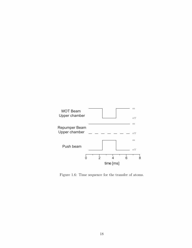
We have transfered 87Rb atoms from the top chamber to the science chamber

with an efficiency of more than 50%. A laser pulse with a duration of 2 ms and a

DC power of 0.5 mW transfers momentum to the atoms effectively pushing them

downward out of the trapping region. This “push” laser beam is linearly polarized

and on resonance with the 5S1/2, F = 3 → 5P3/2, F = 4 atomic transition. Just as

16

Table 1.1: Specifications of conflat flanges of science chamber.

Flange Number Description Use

1 6” flange, through holes Microwave cavity

2 4.5” flange, tapped holes MOT beam

3 4.5” flange, tapped holes Atom input


5 6” flange, through holes Microwave cavity

6 1.33” flange, tapped holes Raman beam

7 6” flange, tapped holes MOT beam

8 1.33” flange, tapped holes Dipole trap

9 1.33” flange, tapped holes Free




13 6” flange, tapped holes MOT beam






17

0 2 4 6 8

Push beam

time [ms]

MOT Beam

Upper chamber

Repumper Beam

Upper chamber

Figure 1.6: Time sequence for the transfer of atoms.

18

the push laser displaces the atoms, we turn off the MOT beams while leaving the

repumper beam on. See Fig. 1.6 for the time sequence.

Figures 1.7 and 1.8 show the fluorescence of the rubidium atoms in both trap-

ping chambers as a function of time. Fig. 1.7 is the fluorescence from the top

chamber. A sudden decrease in the fluorescence marks when the pushing laser

“kicks” the atoms downward. Almost simultaneously, the fluorescence of the sci-

ence chamber (Fig. 1.8) increases: the atoms have been transfered (a 70 cm long

path) to the center of the science chamber.

We calculate the number of atoms inside a radius r0 = 0.5 cm (inner radius of

the differential pumping system) as a function of time using two different procedures

to simulate the transfer process and understand better our losses. In both of them

we model the atomic sample as a non-interacting gas that is randomly distributed

in a sphere with a radius of 100 µm (estimated radius of the MOT) and with a

temperature T= 150 µK. After the push beam interacts with it, the atoms acquire

a velocity V0 in the −z direction. The transverse velocity still obeys a Maxwell

distribution. The first calculation consists of a Montecarlo simulation of the system,

the second one is an analytical solution to the problem. Both of these approaches

give results that are in very good agreement with each other (see Table 1.2) and are

in close agreement with the experimental result. The initial velocities employed in

the calculation are consistent with previous measurements of pushing velocities [8]

However, further work is still necessary to try to maximize the efficiency. Possible

issues that might be limiting our current values could be optical pumping to the

other hyperfine ground state, temperature of the sample and deflection of the atoms

19

0 20 40 60 80

0

1

2

3

4

5

6

7

Flu

ore

sce

nce

[arb

. units

]

time [s]

X104

Figure 1.7: Atomic fluorescence in upper chamber as a function of time.The arrow shows the instant when the push beam displaces the atoms forthe first time towards the science chamber. The increase of fluorescenceis due to reloading of the MOT from the rubidium vapour provided bythe getters. The diference in timing with Fig. 1.8 is due to the CCDcameras being activated at different times.

20

0 10 20 30 40 50

0

1

2

3

4

5

6

Flu

ore

sce

nce

[arb

. units

]

time [s]

X104

Figure 1.8: Atomic fluorescence in science chamber as a function oftime. The arrow shows the instant when the atoms are recaptured inthe science chamber after being pushed by the laser beam for the firsttime. Ech subsequent increase of fluorescence corresponds to a successfultransfer of rubidium atoms. The observed losses are due most probablyto collisions with background gas. The diference in timing with Fig. 1.7is due to the CCD cameras being activated at different times.

21

Table 1.2: Number of atoms at T=150 µK that remain within the area defined

by the inner radius of the differential pumping system (r0 = 0.5 cm). V1 and V2

correspond to calculations considering 20 m/s and 15 m/s as an initial velocity in

the −z direction, respectively. The subindex A and M denotes an analytical or a

Montecarlo solution to the problem.

Falling distance [in] %V1

A %V1

A %V2

MC %V0

MC

3.2 100 100 100 100

6.9 99.99 100 99.8 100

8.6 99.94 99.9 98.5 98.7

12.7 96.7 95.8 85.5 85.4

17.0 85.0 84.7 65.9 66.5

25.2 58 59.2 39.1 37

by other laser beams [21] .

22

Chapter 2

Measurement of the hyperfine splitting of the 6s state of rubidium

2.1 Introduction

High precision measurements of hyperfine splittings are excellent testbeds for

studies of the interaction between the atomic cloud and the nucleus [11, 22, 23,

24, 25, 26, 27]. Since the probability of the electron being inside the nucleus is

nonzero, the electron becomes an excellent probe to explore fine details of interaction

between them such as changes in nuclear matter distribution between isotopes. In

addition, hyperfine splitting measurements represent ideal benchmarks for the ab

initio calculations of the electronic wave function at distances close to the nucleus.

Measurements of hyperfine splittings are also important for studies of atomic

parity non-conservation. Experiments of atomic PNC rely heavily on high precision

calculations (better than 1% error) of operator expectation values to extract from

the experimental data information on the weak interaction [28, 29, 30]. In the case of

cesium, the value of the weak charge extracted from the experiment and the theory

has yielded excellent agreement with the standard model [5, 31].

This chapter presents the measurement of the hyperfine splitting of the 6S1/2

level in 85Rb and 87Rb. The quality of the data allows us to extract, with the values

of the gyromagnetic factors of both isotopes, an isotopic difference in the electronic

wave function evaluated at the nucleus i.e. a hyperfine anomaly. The difference is in

23

excellent agreement with the one extracted from the ground state. Our experimental

results are also in excellent agreement with theoretical prediction of MBPT of the

hyperfine splittings.

This chapter starts with a brief introduction followed by the theoretical back-

ground in Section 2.2. Section 2.3 explains the experimental setup and method to

measure the separation. This section also contains the experimental results and the

results of the search of probable systematics. Section 2.4 compares our results with

theory and Section 2.5 has the conclusions.


2.2.1 Hyperfine interaction

The hyperfine interaction is accounted for by the interplay between the elec-

tromagnetic fields generated by the atomic cloud and the nuclear moments. Two

types of nucleus-electron interactions, though, suffice to account for the interaction

in most atoms. The largest of the contributions comes from the nuclear magnetic

dipole coupling to the magnetic field created by the electrons at the nucleus. The

second one arises from the interaction between the nuclear electric quadrupole and

the gradient of the electric field generated by the electrons at the nucleus. The latter

vanishes for spherically symmetric charge distributions (J, I = 1/2). The hyperfine

energy shift EHF for these levels is [32]:

EHF =A

2(F (F + 1) − I(I + 1) − J(J + 1)), (2.1)

24

where F is the total angular momentum, I is the nuclear spin and A is the magnetic

dipole interaction constant. The derivation of A for a hydrogen-like atom by Fermi

and Segre assumes a point nuclear magnetic dipole [33]

Apoint =16π

3

µ0

4πhgIµNµB|ψ(0)|2, (2.2)

where ψ(0) is the electronic wave function evaluated at the nucleus, µB is the Bohr

magneton, µN is the nuclear magneton and gI is the nuclear gyromagnetic factor.

Under an external magnetic field, the atom acquires an extra potential energy

coming from the alignment of the nuclear magnetic dipole with this field. For small

values of the field (gFµBB/EHF ≪ 1) F is a good quantum number and the energy

of the system is given by

EHF (B) = EHF (0) + gFµBmFB, (2.3)

where gF is the total g-factor, mF is the magnetic quantum number, B is the

magnetic field and EHF (0) is the value of the energy at zero magnetic field. In this

regime of small splittings compared to EHF (0), gF is given by:

gF = gJF (F + 1) + J(J + 1) − I(I + 1)

2F (F + 1)−

gIF (F + 1) + I(I + 1) − J(J + 1)

2F (F + 1),

where gJ is the electronic g-factor.

25

2.2.2 Ab initio calculations

A thorough study of the hyperfine interaction must approach the problem

from a relativistic standpoint which further complicates the problem in a multi-

electron atom. In recent years relativistic many-body perturbation theory (MBPT)

has shown itself to be a powerful and systematic way of extracting, from the high

quality wave functions that it generates, precise atomic properties such as hyperfine

splittings [34, 35].

The full method is outlined in Refs. [36, 37] and references therein. Briefly,

the method, applied to alkali atoms, consists of evaluating a no-pair relativistic

Hamiltonian with Coulomb interactions with a frozen core wave function of a one-

valence electron atom. The Hamiltonian includes projection operators to positive

energy states of the Dirac Hamiltonian. Their presence gives normalizable, bound

state solutions. The wave function contains single and double excitations to all

orders; these correspond to wave functions useful for calculating energy levels and

transition matrix elements. In order to calculate accurate hyperfine constants a set

of triple excitations has to be added. The evaluation of the wave function yields

coupled equations that are solved iteratively for the excitation coefficients which are

then used to obtain atomic properties. Predictions of the theory when the triple

excitations are added are labeled single-double partial triple (SDpT) [34].

The increase in experimental precision in measurements of hyperfine splittings

and the disagreement between theory and experiment of values of hyperfine split-

tings of d states has motivated theorist to include nonlinear coupled-cluster terms.

26

The disagreement stresses the importance of correlations between the electrons in

higher excited states. The inclusion of all valence and core nonlinear coupled-cluster

corrections to the once and twice excited equations allows to take into account the

correlation effects with the predictions labeled coupled-cluster single-double (CCSD)

[35].

The calculations of the hyperfine constants in the SDpT theory are corrected

for the finite size of the nuclear magnetic moment up to zeroth order only due to

their small size in the lighter alkalies (Na, K, Rb). In cesium and francium the

correction becomes more important and is included to all orders. The calculation

ignores isotopic changes of the magnetization distribution and it is modeled as a

uniformly magnetized sphere for all the atoms. The magnetization radius is equal

to the charge radius and the neutron skin contribution is ignored 1. The CCSD

theory considers the nuclear magnetization density as a Fermi distribution with

half-density radius c and 90% - 10% falloff thickness t=2.3 fm [35].

1Knowledge of the neutron skin ∆Rnp, defined as the difference between the rms radii Rn

and Rp of neutron and proton distributions, becomes important in calculations of parity violating

amplitudes. The induced theoretical uncertainty ∆Rnp induced an error that was of the same order

of magnitude as the experimental error in the cesium work [5]. New calculations by Brown et al.

show that the effect is better understood and place an upper correction to the parity violating

amplitude in francium of 0.6% [38].

27

2.2.3 Hyperfine anomalies

The atomic electron sees the nucleus, most of the time, as a structureless

entity with a single relevant parameter, its charge Z. We should expect, hence, the

electronic wave functions of different isotopes, to a very good approximation, to be

the same. It follows then, using Eq. 2.2 that the ratios of electronic wavefunctions,

for the most abundant isotopes of rubidium, should be the same

A87point

A85point

=g87

I

g85I

, (2.4)

where the superindex denotes the atomic number of the isotope.

However, high precision experiments show differences or anomalies from this

description. The nucleus is an extended structured intetity with specific finite mag-

netization and electric charge distributions for each isotope. We can express de-

viations from the point interaction by writing the magnetic dipole constant of an

extended nucleus Aext as a small correction to Apoint [33]

Aext = ApointfR(1 + ǫBCRS)(1 + ǫBW ),

(2.5)

where fR represents the relativistic correction. The last two terms in parenthesis

modify the hyperfine interaction to account for an extended nucleus. The Breit-

Crawford-Rosenthal-Schawlow (BCRS) correction [39, 40, 41], the largest of the two,

modifies the electronic wave function inside the nucleus as a function of the specific

details of the nuclear charge distribution. The second one, the Bohr-Weisskopf (BW)

28

correction [42], describes the influence on the hyperfine interaction of the finite space

distribution of the nuclear magnetization.

Up till now, extraction of ǫBCRS and ǫBW from experimental values has not

been possible due to limits on the theoretical precision. However, the anomalies

can still be observed from the measurements of the magnetic dipole constants in

different isotopes and the values of the g-factors [43, 44]. Deviations from Eq. 2.4

are expressed in terms of the hyperfine anomaly difference 87δ85:

A87g85I

A85g87I

∼= 1 +87 δ85, (2.6)

with 87δ85 = ǫ87BW − ǫ85BW + ǫ87BRCS − ǫ85BRCS . A 87δ85 6= 0 indicates the presence of a

hyperfine anomaly.

2.2.4 Breit-Crawford-Rosenthal-Schawlow effect

The interaction between an electron and an atomic nucleus is precisely de-

scribed by the Coulomb potential when both of them are far away from each other,

no matter whether the nucleus is a point or an extended source. For interactions

that require the nucleus and the electron to be very close to each other, an 1/r po-

tential is no longer adequate. The correction to the electronic wave function due to

the modified nuclear potential is known as the Breit-Crawford-Rosenthal-Schawlow

correction.

Calculations of ǫBRCS take into consideration how the charge is distributed

over the nucleus. Rosenthal and Breit considered for their calculation the charge

29

82 84 86 88 90 92

4.20

4.25

4.30

<r2

>1/2 [fm

]

A

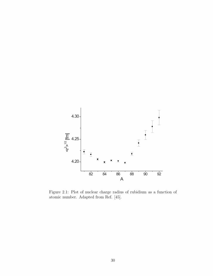
Figure 2.1: Plot of nuclear charge radius of rubidium as a function ofatomic number. Adapted from Ref. [45].

30

rN [fm] Ref. ǫBCRS

85Rb 4.2031(18) [45] 0.0090835(34)

87Rb 4.1981(17) [45] 0.0090735(36)

Table 2.1: Values of ǫBCRS and corresponding nuclear radius for both rubidium

isotopes.

to be on the surface of the nucleus [39]. Schawlow and Crawford also calculated

the change of the wave function except they considered the charge to be uniformly

distributed in the nucleus [40]. Rosenberg and Stroke proposed later a third model

to improve the agreement between theory and experiment: a diffuse nuclear charge

distribution [41].

The neutron and proton shells in rubidium determine the deformation as well

as the spatial distribution of the nuclear charge. The neutron shell for 87Rb is closed

at magic number N = 50 making it impervious to the addition and subtraction

of nuclear matter [45, 46]. The substraction of two neutrons to form 85Rb does

not affect significantly the electric charge distribution, and the electric potential,

compared to the one from 87Rb, remains the same (see Fig. 2.1).

The expression of ǫBCRS for the uniformly charged sphere and charge on surface

models is [47]:

ǫBCRS =2(κ+ ρ)ρ(2ρ+ 1)

(2κ+ 1)(Γ(2ρ+ 1))2(pZrN

a0)2ρ−1, (2.7)

where p is a constant of order unity, ρ =√

κ2 − (Zα)2, a0 and α are the Bohr radius

and fine structure constant, respectively, rN is the nuclear radius, and κ is related

31

to the electronic angular momentum through the equation κ = 1+J(J+1)−L(L+

1)−S(S+1). Table 2.1 shows the value of the correction for a uniformly distributed

charge as well as the nuclear radius of each isotope employed in the calculation.

Rosenfeld and Stroke propose a trapezoidal charge distribution to approximate

their model. The interested reader should consult Ref. [41] for further explanation.

All three models give relatively large ǫBCRS (∼1%), however, the difference between

both isotopes for all models is very small: ǫ87BCRS − ǫ85BCRS ∼ 10−5.

2.2.5 Bohr-Weisskopf effect

The interplay between nuclear magnetization with the magnetic field created

by the atomic electrons causes the hyperfine splitting in atoms. A natural extension

of hyperfine splitting measurements is to compare models of nuclear magnetism.

Nuclear magnetization is described in terms of nuclear moments with the

biggest contribution coming from the nuclear magnetic dipole moment. The as-

sumption of a point magnetic dipole gives good agreement between calculations and

experiment, however it does not provide the complete picture. Nuclear magnetiza-

tion has a finite volume. The electron wavefunctions of levels with total angular

momentum J = 1/2 have a bigger overlap with the nucleus and are able to expe-

rience the subtle changes of the spatial distribution of the nuclear magnetization.

These wave functions need to be modified to correctly account for the hyperfine

splitting.

The corrections ǫBW to the wave functions due to a finite magnetization distri-

32

bution were first computed by Bohr and Weisskopf [42]. They assumed a uniformly

distributed magnetization over the nucleus for their calculation with a predicted

ǫ87BW − ǫ85BW that ranges between 0.11% and 0.29%. The BW correction roughly

scales as [42]:

ǫBW ∼ (ZrN

a0)(

a0

2ZrN)2(1−

√1−(Zα)2)(

r2

r2N

)Av, (2.8)

where the average is taken over the magnetization distribution, with (r2/r2N)Av =

3/5 for a uniform magnetization. For rubidium this gives a correction of the order

of 0.2%, however it is strongly dependent on spin and orbital states of the nucleons

i.e. on the specifics of the nuclear magnetization. Stroke et. al. performed the

same calculation using a trapezoidal magnetization distribution [48]. Their results

agree very well with experimental information extracted from the ground state; they

calculate a hyperfine anomaly difference of 0.33%. Both of these theoretical results

are independent for the main quantum number of the valence electron [33], just as

required by Bohr and Weisskopf.

The nuclear shell model predicts that the total magnetic dipole moment has

contributions from both the proton and the neutron shell, each with orbital and

spin angular momenta [33]

~µ =∑

i=n,p

(geffs,i ~si + geff

l,i~li)µN , (2.9)

where geffs and geff

l are the effective nuclear spin and nuclear orbital gyromagnetic

ratios, respectively, ~s and ~l are the nuclear spin and nuclear orbital angular momenta

33

Theory [µN ] Experiment [µN ] Ref.

85Rb 2.00 1.35298(10) [50]

87Rb 2.64 2.75131(12) [50]

Table 2.2: Theoretical and experimental values of the nuclear dipole moment for

rubidium.

and the sum is taken over both shells. The g-factors have the values geffs =3.1(2)

and geffl =1.09(2) [49].

The magnetic dipole moment in rubidium comes almost entirely from the vec-

tor addition of the orbital and spin angular momenta of a single valance proton. The

neutron shell is almost spherical for both isotopes due to its closed shell structure

and the contribution to the angular momentum from the neutron shell is very small.

The lighter of the two isotopes, 85Rb, has the valence proton in an almost

degenerate f orbital with its spin and orbital momenta antialigned yielding a value

of I=5/2. Adding two more neutrons to the core shifts the energy level of the

valence proton to the nearby p orbital and aligns both momenta giving the known

value of I=3/2. Table 2.2 presents the theoretical prediction of the nuclear magnetic

moment using Eq. 2.9 as well as the experimental result. It is indeed remarkable

that such a simple model reproduces closely the experimental results, particularly

for the closed nuclear shell structure of 87Rb.

Three main factors make the two stable isotopes of rubidium good candidates

for observing the BW effect. First the different orientation of the nuclear spin of the

valence proton with respect to the nuclear orbital angular momentum. Second, the

34

small relative difference in nuclear charge deformation. Third, the change of orbital

for the valence proton in the two isotopes.

2.2.6 Two-photon spectroscopy

We use atomic laser spectroscopy to measure the hyperfine splitting in two

isotopes of rubidium. To reach the 6S1/2 state from the 5S1/2 ground state we need

a two photon transition. We increase the probability of transition by using the

5P1/2 level as an intermediate step. We develop a theoretical model of the two-

photon transition that includes the main physical aspects of our atomic system (see

Fig. 2.2) based on a density matrix formalism.

Our experimental setup consists of two counter propagating laser beams going

through a glass cell with rubidium vapor in a small magnetic field. We lock the

laser at 795 nm on resonance, the middle step to the 5P1/2 level, while we scan the

1.324 µm laser (from here on referred to as the 1.3 µm laser) over the 6S1/2 level

and observe the absorption of the 795 nm laser. The system can be modeled as a

three level atom in which the on-resonance middle step enhances the excitation to

the final step and the counter propagating laser beams help suppress the Doppler

background (see for example Ref. [51]). However, numerical simulations show that

we have to model our system as a five level atom to include its main qualitative

feature: optical pumping effects increase the absorption of the 795 nm laser when

the 1.3 µm laser is on resonance.

Figure 2.3 shows our simplified atomic model. We have neglected the Doppler

35

F=3 (2)

F=2 (1)

F=2 (1)5S

1/2

F=3 (2)5P

1/2

6S1/2

F=4 (3)

F=3 (2)5P3/2

F=2 (1)

F=1 (0)

F=3 (2)

F=2 (1)

795 nm

1.324 μm

Figure 2.2: Energy levels relevant to our experiment (energy separationsnot drawn to scale). The numbers correspond to 85Rb (87Rb). Straightarrows correspond to the excitation lasers, ondulated arrows to decays.

36

1>

5>

4>

3>

2>

α 12 γ

21

γ25

γ32

γ34

γ41 γ

45

α 23

γ51

δ 23

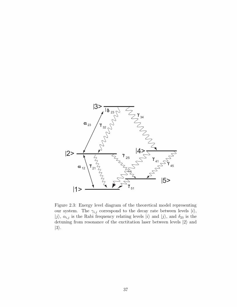
Figure 2.3: Energy level diagram of the theoretical model representingour system. The γi,j correspond to the decay rate between levels |i〉,|j〉, αi,j is the Rabi frequency relating levels |i〉 and |j〉, and δ23 is thedetuning from resonance of the exctitation laser between levels |2〉 and|3〉.

37

effects as well as the Zeeman sublevels in order to keep the calculation as simple

as possible without losing the main qualitatively features of our system. Level |1〉

represents the lower hyperfine state of the 5S1/2 level while |2〉 is the upper hyperfine

state of the 5P1/2. The decay rate between the two levels is γ21/2π = 6 MHz [52].

We simplify the hyperfine states of the 6S1/2 level to just one level with decay rate

γ32/2π = 3.5 MHz [53]. The ground and intermediate levels are coupled by the

Rabi frequency α12 while the intermediate and the excited levels are coupled by α23.

The remaining two levels, |4〉 and |5〉, represent all other decay channels out of the

cascade system and the upper hyperfine ground level, respectively. The detuning

between levels |1〉 and |2〉 is zero for our experiment, but we let the detuning between

levels |2〉 and |3〉 vary as δ23. The total population is normalized to one.

We are left with a set of twenty five linear equations for the slowly varying

elements of the density matrix σnm after using the rotating wave approximation.

These are

∑

k

(γknσkk − γnkσnn) + (2.10)

i

2

∑

k

(αnkσkn − σnkαkn) = 0 for n = m,

[i(Ωnm − ωnm) − Γnm)]σnm + (2.11)

i

2

∑

k

(αnkσkm − σnkαkm) = 0 for n 6= m,

where ωnm = (En − Em)/h is the transition frequency, Ωnm = −Ωmn is the laser

frequency connecting the levels. The damping rate is given by:

Γnm =1

2

∑

k

(γnk + γmk). (2.12)

38

0.0436

0.0438

0.044

0.0442

δ / γ23

Ab

sorp

tio

n [

arb

. un

its]

-100 -50 0 50 100

0.0424

0.0428

0.0432

0.0436

a)

b)

0

0

21

Figure 2.4: Numerical simulation of the absorption of the 795 nm laseras a function of the normalized detuning of the 1.3 µm laser to level |3〉in units of γ21. Both plots have the same parameters except for the ratioγ41/γ45. (a) Increase of absorption with γ41/γ45 = 2. (b) Decrease ofabsorption with γ41/γ45 = 1/2.

39

We solve for σ12 leaving the detuning between levels |2〉 and |3〉 (δ23 = Ω23−ω23)

as a free parameter. We plot the negative of the imaginary part of σ12, which is

proportional to the absorption of level |2〉, as a function of δ23 for several different sets

of parameters. Our five level model reproduces the increase of absorption observed

as the second excitation goes into resonance. This can be explained in the following

way. The laser coupling levels |1〉 and |2〉, in the absence of the second excitation,

pumps the atoms to level |5〉. In the steady state there will be little absorption due

to a very small number of atoms being transferred from |5〉 to |1〉. By adding the

second excitation a new reservoir of “fresh” unexcited atoms appears in level |1〉.

Instead of falling to the non-absorbing level |5〉, they travel to level |3〉 and then

decay to the initial ground state level through level |4〉. These “fresh” atoms will

add to the ground state population and increase the absorption (see the Appendix).

Figure 2.4 shows samples of our simulation. We have plotted the absorption

of the laser connecting levels |1〉 and |2〉 as a function of the detuning of the second

laser. Figure 2.4 (a) shows how the absorption increases as the second laser goes

on resonance while Fig. 2.4 (b) shows a decrease. Both plots have the same model

parameters except for the ratio γ41/γ45. This ratio determines whether the atom will

be lost or return to the cycle. A ratio bigger than one pumps atoms preferentially to

level |1〉 rather than level |5〉 which constitutes a fresh reservoir of excitable atoms.

40

795 nm laser

1.3

μm

lase

r

P.D.H. lock

Modulator

Amplifier

Rb

ce

ll

M. sh

ield

λ/4

λ/4

PD

PD

BS

BS

M. co

ils

Figure 2.5: Block diagram of the experiment. Key for figure PD: photo-diode, P.D.H.: Pound-Drever-Hall, M: magnetic, BS: beamsplitter.

41

2.3 Measurement of the hyperfine splitting

2.3.1 Apparatus

We use a Coherent 899-01 Titanium Sapphire (Ti:sapph) laser with a linewidth

of better than 500 kHz tuned to the D1 line at 795 nm for the first step of the

transition. A Pound-Drever-Hall (PDH) lock to the F = 1(2) → F = 2(3) transition

in 87Rb (85Rb) in a separate glass cell at room temperature stabilizes the linewidth

and keeps the 795 nm laser on resonance. An HP 8640B signal generator acts as the

local oscillator for the lock. The 795 nm laser remains on resonance for about 40

minutes, much longer than the time it takes to record a single experimental trace.

A grating narrowed diode laser at 1.3 µm with a linewidth better than 500 kHz

excites the second transition. We scan the frequency of the 1.3 µm laser with a tri-

angular shaped voltage ramp from a synthesized function generator at 4 Hz applied

to the piezo control of the grating and monitor its frequency with a wavemeter with

a precision of ±0.001 cm−1. A fiber-coupled semiconductor amplifier increases the

power of the 1.3 µm laser before it goes to a large bandwidth (≈10 GHz) Electro-

Optic Modulator (EOM). Another HP 8640B modulates this EOM. Fig. 2.5 shows

a block diagram of the experimental setup.

A thick glass plate splits the 795 nm laser beam into two copropagating beams

before going to the glass cell. The glass cell is 30 cm long and has a diameter of

2.5 cm. The rubidium glass cell was made at NIST using high vacuum and a

99.9% pure rubidium ampoule to minimize contaminants and with no buffer gas.

The power of each beam is approximately 10 µW with a diameter of 1 mm. We

42

500 1000 1500 2000 2500

0.00

0.01

0.02

0.03

0.04

F=1

F=2

Abso

rptio

n [A

rb. units

]

Frequency [MHz]

sidebands

Figure 2.6: Absorption profile of the 6S1/2, F = 1 and F = 2 hyperfinestates of 87Rb with sidebands. The big sideband belongs to the F = 1peak. The small feature on the side of the F = 2 peak corresponds tothe second sideband of theF = 1 peak. The glass cell is in a magneticfield of 0.37 G.

43

operate in the low intensity regime to avoid power broadening, differential AC stark

shifts and line splitting effects such as the Autler-Townes splitting. Both beams are

circularly polarized by a λ/4 waveplate. A counter propagating 1.3 µm laser beam

with a power of 4 mW and approximately equal diameter overlaps one of the 795 nm

beams. The lasers overlap to a precision of better than 1 mm along 75 cm giving at

most a diverging angle of 1 mrad.

The cell resides in the center of a 500-turn solenoid that provides a magnetic

field of 7.4 Gauss/A contained inside a three layered magnetic shield to minimize

magnetic field fluctuations [54]. The middle layer has a higher magnetic permeability

to avoid saturation effects. The dimensions of the solenoid (70 cm long and a

diameter of 11.5 cm) guarantees the uniformity of the magnetic field observed by

the atoms. We operate under a weak magnetic field (B ≈1 Gauss) to work in the

Zeeman linear regime.

After the glass cell an independent photodiode detects each 795 nm beam.

The outputs of the detectors go to a home-made differential amplifier to reduce

common mode noise. A digital oscilloscope records the output signal for different

values of modulation, polarization and magnetic field and averages for about three

minutes. The order in which the absorption profiles are recorded is random. During

the experimental runs we monitor the current going to the solenoid that provides

the quantization axis. A thermocouple measures the changes in temperature inside

the magnetic shield (24oC) to within one degree. The optical attenuation for the

D1 line at line center is 0.4 for 85Rb and about three times less for 87Rb.

44

2.3.2 Method

We modulate the 1.3 µm laser to add sidebands at an appropriate frequency

with a modulation depth (ratio of sideband amplitude to carrier amplitude) that

ranges between 1 and 0.1. The sidebands appear in the absorption profile at a

distance equal to the modulation from the main features and work as an in situ

scale (see Fig. 2.6). We measure their separation as a function of the modulation

for values bigger and smaller than half the hyperfine splitting. We interpolate to

zero separation to obtain half the hyperfine splitting (see Fig. 2.7). This technique

transfers an optical frequency measurement to a much easier frequency measurement

in the RF range.

The size of the main peaks depends on the coupling strength between transi-

tions; the size of the sidebands (as compared to the main peaks) will be determined

by the strength of the transition and also on the number of sidebands simultaneously

on or close to resonance. We observe under normal experimental conditions that

the laser sidebands are both close to resonance (the lower frequency sideband to the

6S1/2 F = 1 and the upper one to the F=2 transition) when the carrier is around

the half point of the splitting. The stronger of the transitions (F = 1) depopulates

the 5P1/2, F = 2 level leaving only a few atoms to excite with the upper sideband,

hence the smaller transmission peak for the sideband corresponding to F = 2.

We have also observed a much richer atomic behavior by changing the laser

intensities, polarizations and magnetic field environment of the glass cell. Optical

pumping moves the atomic population from one level to another quite efficiently.

45

0.1

0.2

]sti

nu .

brA[

noit

pro

sb

A

300

350

400

Modulation [MHz]

-100

0

100

Frequency [MHz]

Figure 2.7: Experimental traces that illustrate sideband crossing for85Rb. The larger resonance corresponds to the F = 2 level, the smallerone to the F = 3 level of the 6S1/2 state. The dots correspond to thecenter of the profiles, the point where both lines cross corresponds tohalf the hyperfine separation.

46

- 0.005

0.000

0.005

0.010

Ab

sorp

tio

n [

arb

. un

its]

- 0.015

0.015

0.0 2.0 4.0

Frequency [GHz]

F=2

F=1

Figure 2.8: Experimental trace of absorption of the 795 nm laser for87Rb showing both increase and decrease of absorption due to opticalpumping.

47

This is manifest in how the peaks change in magnitude or just switch from an

increase of absorption to a decrease (see Fig. 2.8) just as our very simple theoretical

model predicts. These effects point out that a careful control of the environment is

necessary for a successful realization of the experiment.

The transfer of population by specific selection of polarization and magnetic

environment can also be used to obtain a better experimental signal. There are

several options to reach the 6S1/2 level. From the ground hyperfine states we can

do ∆F = 0,±1 transitions. We find that doing the two step excitation in either

a σ+ : σ− or σ− : σ+ polarization sequence for the 795 nm and 1.3 µm lasers,

respectively, with a ∆F = 1 for the first step increases the amplitude of the signal.

By choosing this polarization sequence we increase the probability of the atom going

to the excited state and avoid placing it in a non-absorbing state [55].

We place the rubidium cell in a uniform magnetic field collinear with the prop-

agation vectors of both lasers. The magnetic field provides a quantization axis as

well as a tool to probe systematic effects. The hyperfine separation is now dependent

on the magnetic field strength and the alignment with the laser. We measure the

hyperfine splitting for different values of the magnetic field and polarization making

sure that the above polarization sequence is always satisfied. We extract the value

of the splitting at zero magnetic field from a plot of hyperfine splitting as a function

of magnetic field.

48

0.000

0.001

0.002

Abso

rptio

n [A

rb. units

]

0.003

0.004

0.005

0.006

-4

-3

-2-1

0

12

3

4

Resi

dues/

Err

or

Resi

dues/

Err

or

0

5

10

15

-5

-10

-15

300 350 400 450

Frequency [MHz]

a)

b)

c)

X X1 2

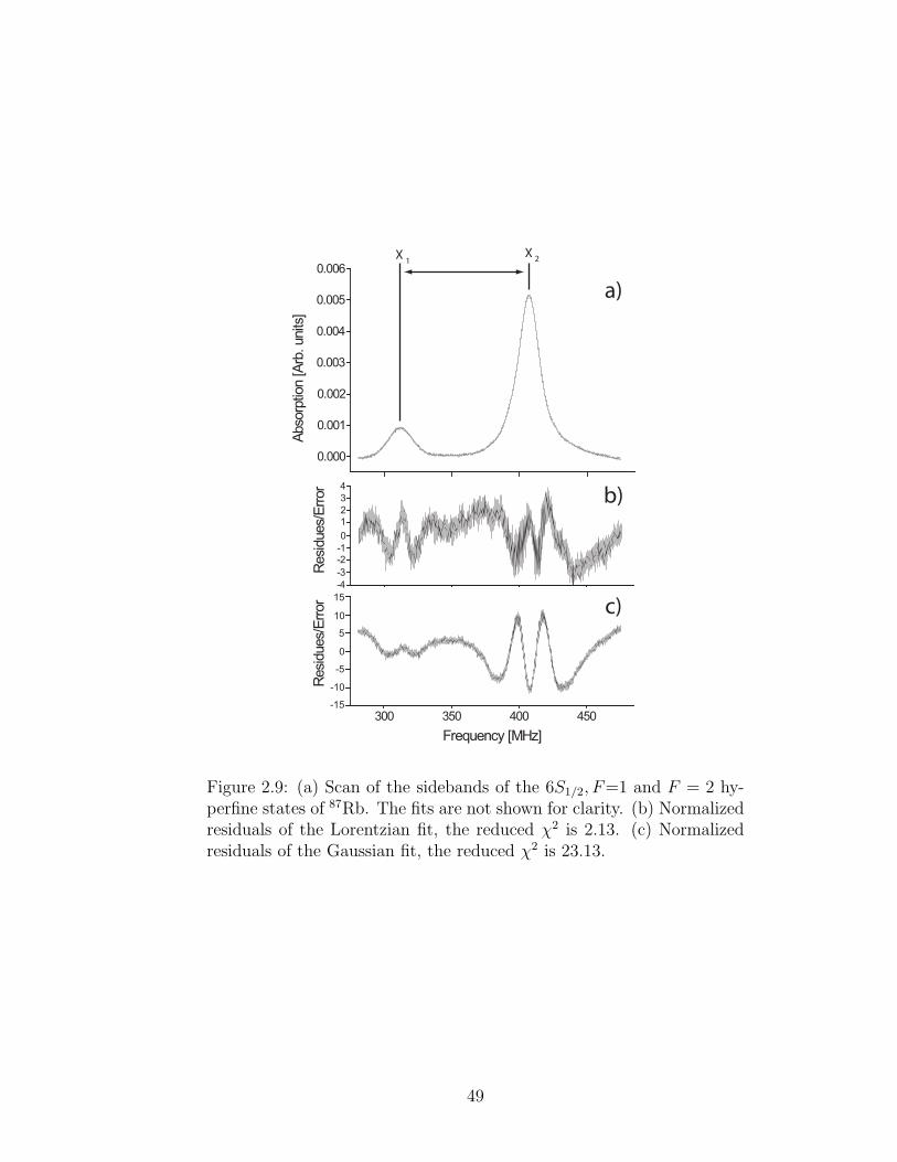
Figure 2.9: (a) Scan of the sidebands of the 6S1/2, F=1 and F = 2 hy-perfine states of 87Rb. The fits are not shown for clarity. (b) Normalizedresiduals of the Lorentzian fit, the reduced χ2 is 2.13. (c) Normalizedresiduals of the Gaussian fit, the reduced χ2 is 23.13.

49

2.3.3 Results and systematic effects

We study the contributions of several systematic effects that can influence the

hyperfine separation measurement. We analyze the peak shape model for the non-

linear fit to obtain the separation of the centers of the profiles, scan width and scan

rate of the 1.3 µm laser, power of the 795 nm and 1.3 µm lasers, optical pumping

effects, magnetic field effects, and temperature.

A)Peak shape model and non-linear fit. The absorption of a Doppler-broadened

two level system as a function of laser detuning is a Voigt profile. When a multi-

level system is considered it is not trivial to write down the functional form of the

absorption of any of the lasers interacting with the system (see for example Refs.

[56, 57]). We fit the experimental data to Voigt, Lorentzian and Gaussian functions

to find the line centers and compare the results for consistency.

We use the non-linear fit package of ORIGINTM to fit the above mentioned

profiles to search for model-dependent systematics. ORIGINTM uses a Levenberg-

Marquardt algorithm to minimize the residuals given a specified error. The program

has been used in the past by our group to obtain high precision lifetime measure-

ments [14, 53]. We use the resolution limit of the 8 bit analog to digital converter

of the scope for these calculations which corresponds to 0.5% of the total scale

used. Lorentzian and Gaussian fits have three variable parameters to fit for each

peak which correspond to the FWHM, the line center, the area under the curve

plus a single offset for both peaks. Voigt profiles have an extra parameter which

corresponds to the temperature of the sample. ORIGINTM gives the error of each

50

parameter which depends on the quality of the data.

Voigt profiles are in very good agreement with the lineshape. The fit yields

the low temperature limit of the Voigt profile i.e. a Lorentzian, and hence is in

agreement with the line center extracted using a Lorentzian profile. This is expected

since the contribution of the Doppler effect to the resonance lineshape should be

minimized by the counter propagating laser setup and by an expected group velocity

selection arising from the the two-step excitation process i.e “two-color hole burning”

(see Appendix A). The 795 nm laser will only interact with a small number of group

velocities; these groups will be the only ones that will be excited to the 6S1/2 level

by the 1.3 µm laser. Line centers extracted from Gaussian fits agree with results

from the above mentioned profiles but decay too fast for frequencies far away from

the centers. We also fit the data to a convolution of Lorentzian profiles with a

rectangular transmission function and an exponential of a Lorentzian to search for

systematic errors and to understand better our residues.

All peak shape models give consistent line centers consistent among them-

selves. All of them have similar structures in the residues within the line width of

the resonances (see Fig. 2.9). We have determined that these features come about

from the high sensitivity from deviations from a perfect fit that a difference of two

peak profiles has. In other words, by taking the residues we are effectively taking

the derivative of a peak profile that will be as sensitive as sharp the linewidth is. To

further verify this we take the numerical derivative of the data to search for residual

structure that might change our measurement (see Fig. 2.10). We fit a straight line

to the data that lies within the linewidth and extract when the line crosses zero.

51

The results are consistent with the fits. Close analysis of the derivative in this region

reveals no structure.

Of the fitted functions Lorentzians yield the smallest χ2. The fitting error of

the line centers for all our data for Lorentzian fits range between 15 kHz and 30

kHz. We quote the average of all the fitting errors of our data in Table 2.3. Fig. 2.9

shows the magnified sidebands as well as the residues for a Lorentzian and Gaussian

fits. We extract the line centers with both models; the difference in separation for

both models is in this case |x1−x2|Lorentzian−|x1−x2|Gaussian = 0.35(68) MHz. The

reduced χ2 of the non-linear Lorentzian fit for all our data ranges between 1 and 10

depending on the noise of the signal with a χ2 average of 2.4 over twenty fits. We

do not observe changes in the splitting that depend on the frequency range fitted

around the resonances.

The relative angle between both copropagating lasers induces a systematic

shift on the absolute frequency the atoms observe due to the appearance of the ~v · ~ki

dependence on absorption where ~v is the velocity of the atom and ~ki is the wave

vector for either laser. This angle dependence on the Doppler shift for our system

is almost the same for both our lasers since the cosine of the angle between them

differs from one by one part in 105. Furthermore, any residual effect is minimized

since we measure frequency differences.

Just like the lines shape, analytic expressions for the linewidth are difficult to

write down. We perform a numerical simulation of our five level system presented in

Subsection 2.2.6 of the theoretical background in the presence of a room temperature

velocity distribution. The resonances show linewidths of the order of 30-40 MHz

52

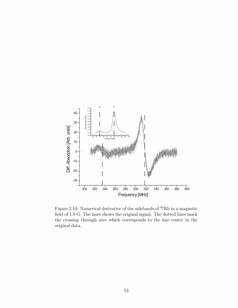
200 220 240 260 280 300 320 340 360 380 400

-30

-20

-10

0

10

20

30

40

Diff

. A

bso

rptio

n [A

rb. units

]

Frequency [MHz]

200 220 240 260 280 300 320 340 360 380 400-0.002

0.000

0.002

0.004

0.006

0.008

0.010

0.012

0.014

0.016

0.018

Abso

rptio

n [A

rb. U

nits

]

Frequency [MHz]

Figure 2.10: Numerical derivative of the sidebands of 85Rb in a magneticfield of 1.8 G. The inset shows the original signal. The dotted lines markthe crossing through zero which corresponds to the line center in theoriginal data.

53

which are in very good agreement with experimental results.

Distortions of the lineshape i.e. asymmetries, depend on the detuning of the

795 nm laser from resonance. These can induce unwanted systematic errors to the

measurement. Numerical simulations show, following Ref. [11], that the separation

of the hyperfine splitting depends negligibly on the detuning from the D1 line.

Nevertheless, we look for any asymmetries in the peaks themselves and dependence

on the direction of scan during experimental runs. No correlation with these effects

is found.

We interpolate to zero from a plot of distance between the center of the side-

bands vs. the modulation frequency to obtain half the hyperfine separation. The

linear regression coefficients in this plots differ from one at the most in 2 parts in

104. Typical errors for the crossovers amount to about 200 kHz.

B)Scan and linearity of 1.3 µm laser. Non-linearities in the piezo driving

the feedback grating, hysteresis effects as well as a slow thermal drift on the 1.3

µm laser can generate undesired systematics in the measurement. We look for non-

linearities by sending the voltage monitor of the piezo to a digital scope with an 8-bit

resolution during the experimental runs as well as monitor the absorption peaks for

asymmetries. Comparison between absorption peaks for both types of scan (low to

high frequency and vice versa) reveals no systematic effects. Analysis of the long

term drift of the 1.3 µm laser shows a stability of better than 100 kHz over a 5

min. period which is longer than the time we need to take a single experimental

absorption signal.

C)Power of the 795 nm and 1.3 µm laser. We look for systematic dependence

54

-2.0 -1.5 -1.0 -0.5 0.0 0.5 1.0 1.5 2.0

715

716

717

718

719

720

Hyp

erfin

e s

plit

ting (

6S

)

[M

Hz]

B-field [Gauss]

1/2

Figure 2.11: Zeeman plot of the hyperfine separation of the 6S1/2 level of85Rb with both lasers circularly polarized to better than 95% and linearfit.

55

on the hyperfine splitting on the power of both lasers. We change the power of

the 795 nm laser from 4 µW to 40 µW while keeping the power of the 1.3 µm

laser constant. Low signal to noise ratio and the observation of the Autler-Townes

splitting determine the lower and upper boundaries of this interval, respectively.

The Autler-Townes effect predicts a splitting of the middle energy level by the

on-resonance first step in a three level system that is proportional to the square root

of its intensity [58]. For our typical experimental conditions the splitting should be

less than 4 MHz, too small to be resolved with the observed linewidths of the atomic

resonances (∼ 40 MHz).

The 1.3 µm laser operates very close to its maximum power under normal

experimental conditions. The power is distributed among the sidebands and the

main carrier depending on the modulation depth. We gradually decrease the power

of the 1.3 µm to half its operating value to detect any dependence on the power.

We observe no correlation.

D)Optical pumping effects and magnetic field. Optical pumping effects are the

most delicate of all the systematic effects. Both laser beams are carefully polarized

using appropriate λ/4 waveplates and their polarization checked with a rotating

polarizer in front of a detector to better than 95%. The polarization of the lasers

as well as their alignment with the magnetic field determine the relative size of the

peaks (mF sublevels) that form the resonances of the 6S1/2 hyperfine levels. Com-

parison of absorption profiles for a set polarization sequence for different values of

the magnetic field gives qualitative information of the alignment between the mag-

netic field and the lasers. The positive and negative magnetic field orientations in a

56

perfectly symmetric situation, after a switch of polarization sequence, should yield

the same absorption profile. For everyday experimental conditions (around 1 G) we

observe no difference between positive and negative magnetic field directions. We

see broadening of the profiles at magnetic fields twenty times larger but no asym-

metries. Differences start appearing at around 85 G which suggests good alignment

between the lasers and the magnetic field as well as good control of the polarization

of both lasers.

The hyperfine separation vs. magnetic field plot provides more quantitative

information. Eq. (3) states that the plot should be linear with no discontinuities

as we change the value of the magnetic field from positive to negative. Our plots

show a smooth transition between negative and positive values of the magnetic field

within experimental error. Fig. 2.11 shows a sample of our data when both lasers

are circularly polarized to better than 95%.

We monitor the current of the coil generating the magnetic field to detect any

fluctuation in the intensity of the field. We observe small fluctuations of the order

of mG from current noise.

E)Temperature. We analyze the position of the absorption peaks as a function

of temperature of the cell to check for related systematic effects such as collision

shifts for both isotopes. The temperature of the glass cell is increased from room

temperature (23oC) up to 40oC using a heat tape wrapped around it. While record-

ing data we turn off the heating tape to avoid stray magnetic fields generated by the

current going through it. The temperature of the glass cell is monitored with a ther-

mocouple inside the magnetic shield with an accuracy of one degree. No dependence

57

Systematic effects ν85HF [MHz] ν87

HF [MHz]

Optical pumping effects ≤ 0.016 ≤ 0.029

Power of 795 nm laser ≤ 0.020 ≤ 0.005

Power of 1.3 µm laser ≤ 0.011 ≤ 0.011

Atomic density ≤ 0.020 ≤ 0.010

Non linear fit ≤ 0.028 ≤ 0.023

B-field fluctuations ≤ 0.015 ≤ 0.025

Total Systematic ≤ 0.047 ≤ 0.047

Statistical error 0.100 0.160

TOTAL 0.110 0.167

Table 2.3: Error budget for the hyperfine splitting measurement

on temperature is found.

We have concluded after close analysis of these studies that, to the accuracy

of our measurement, Gaussianly distributed statistical fluctuations dominate our

experiment (see Table 2.3). The statistical error in the hyperfine splitting, as stated

by the standard error of the mean, is 110 kHz for 85Rb and 167 kHz for 87Rb.

Figure 2.12 shows the values of the magnetic dipole constant for 85Rb for all

experimental runs of this work. The final result for each run is determined by an

interpolation to zero magnetic field as a function of the current in the solenoid.

Table 2.4 contains the measurements of the hyperfine splitting of the 6S1/2

level as well as the corresponding values of the magnetic dipole constants for both

isotopes.

58

239.05

239.10

239.15

239.20

239.25

239.30

239.35

A (

6S

)

[M

Hz]

85

Run

1 2 3 65 74 8

1/2

Figure 2.12: Results of different runs of the magnetic dipole constantsof the 6S1/2 state of 85Rb. The dashed line corresponds to the mean, thesolid lines to the 1-σ error.

59

85Rb [MHz] 87Rb [MHz]

νHF 717.54(10) 1615.32(16)

A 239.18(03) 807.66(08)

Table 2.4: Hyperfine splittings (νHF ) and magnetic dipole constants for the 6S1/2

level.

The precision of our data allows us to observe a hyperfine anomaly. We use the

values of Ref. [59] for the ratio g85I /g

87I = 0.295055(25). This is consistent with the

experimental values of Ref. [50]. Using this value and our experimental results in

Eq. 2.6 we obtain a value for the hyperfine anomaly difference of 87δ85=-0.0036(2).

This is less than a one percent difference, well beyond the current MBPT theoretical

calculation accuracy of the hyperfine splittings.

2.4 Comparison with theory

We compare in Figs. 2.13 and 2.14 the results from this experiment with the

previous experimental results of Gupta et al. [60] and the theoretical predictions of

Ref. [34]. The hyperfine anomalies are still not within reach of ab initio MBPT so

the value of 85Rb comes from the value of 87Rb considering no hyperfine anomaly.

2.5 Conclusions

We have measured the hyperfine splittings of the 6S1/2 level of 85Rb and 87Rb

to a precision of 103 ppm and 153 ppm, respectively. Our measurement is consistent

60

238

239

240

241

0.25 %

c

b

a

A85 (

6S

)

[M

Hz]

Rb85

1/2

Figure 2.13: Comparison between experimental and theoretical resultsof the magnetic dipole constant of the 6S1/2 state of 85Rb. The pointslabeled “a” and “b” correspond to our work and the work of Ref. [60],respectively. Point “c” corresponds to the theoretical prediction of Ref.[34].

61

804

806

808

810

812

814

0.25 %

d

b

a

A87 (

6S

)

[M

Hz]

Rb87

1/2

Figure 2.14: Comparison between experimental and theoretical resultsof the magnetic dipole constant of the 6S1/2 state of 87Rb. The pointslabeled “a” and “b” correspond to our work and the work of Ref. [60],respectively. Point “d” corresponds to the theoretical prediction of Ref.[34] considering a non extant hyperfine anomaly.

62

SDpT [MHz] CCSD [MHz] Experiment [MHz]

5S1/2 1011.1 1020.086 1011.910813(2) [61]

5P1/2 120.4 119.192 120.499 (10) [22]

6S1/2 238.2 239.18(3) (this work)

6P1/2 39.02 39.11(3) [25, 62]

7S1/2 94.3 94.658(19) [27]

Table 2.5: SDpT and CCSD theoretical predictions calculated using ab intio MBPT

from Ref. [34] and Ref. [35], respectively, and experimental magnetic dipole con-

stants for the first J=1/2 levels in 85Rb.

with and decreases the uncertainty of the past measurements [60] by a factor of 63

for 87Rb and by a factor of 30 for 85Rb [63].

Table 2.5 shows the values of the magnetic dipole constants using relativistic

MBPT [34, 35] with single double partial triple (SDpT) wave functions, coupled-

cluster single-double (CCSD) wave functions, and values extracted from measure-

ments of the hyperfine splitting in other electronic states currently in the literature

for J=1/2 [22, 25, 27, 61, 62]. We have not been able to find in the literature

values for higher levels with adequate precision to include them in the figure. The

agreement of the theory with the experiment, for J=1/2 levels, is well within the

1% level.

We are able to extract the hyperfine anomaly with our experimental data

and show that precision measurements of the hyperfine structure in atomic states

with different radial distributions can give information on the nuclear magnetization

63

5S1/2

5P1/2

6S1/2

6P1/2

7S1/2

0.996

0.997

0.998

0.999

1.000

1.001

A87g

85/A

85g

87

Figure 2.15: Hyperfine anomalies of other atomic levels of rubidiumalong with the value for the 6S1/2 level obtained in this measurement.The dashed line corresponds to the theoretical prediction for a diffusemagnetization distribution [48]. See text for references.

64

87δ85

5S1/2 -0.00356(8) [61]

5P1/2 -0.0001(1) [22]

6S1/2 -0.0036(2) (this work)

6P1/2 0.0000(8) [25, 62]

7S1/2 -0.0032(2) [27]

Table 2.6: Hyperfine anomaly differences 87δ85 for the first J=1/2 levels in rubidium.

distribution. The hyperfine anomaly difference we extract for the 6S1/2 is 87δ85 =

−0.0036(2) [64]. The difference in the anomalies is indeed a factor of thirty larger

than the expected BCRS contribution and it comes from the BW effect. Fig. 2.15

shows that the anomaly measured with the nS1/2 levels is the same independent

of the principal quantum number as well as the smaller deviation from the point

interaction, if any, for the nP1/2 levels [22, 25, 27, 61, 62, 63]. Table 2.6 shows the

hyperfine anomaly differences for the first J = 1/2 levels.

The Bohr-Weisskopf effect predicts that the size of the effect is independent of

the principal quantum number n. The plot and the table confirm this as well as the

larger effect on the S states [42]. These new measurements invite new calculations

of atomic properties and constrain nuclear calculations. As the nuclear charge and

magnetization distribution are better understood they will further test and refine

the calculations which are of crucial importance for PNC experiments.

65

Chapter 3

Measurements of lifetimes of excited states of francium and rubidium

3.1 Introduction

The lifetime of an excited state in an atomic system depends on the expectation

value of the dipole operator e~r between an initial and a final state wave functions

[32]. In addition to being tools for tests of atomic structure, measurements of excited

states lifetimes are the perfect complement for studies of hyperfine splittings since

it is the behavior of the electronic wave function far away from the nucleus that

becomes important. We present in this chapter the measurement of the lifetime of

the 8s excited state in francium and the lifetime of the 5D3/2 state of rubidium.

The measurement of the lifetime of the other state of the 5d manifold, the 5D5/2,

can be found in our recent publication [65].

The 8s state is the preferred candidate for an optical PNC measurement: the

dipole-forbidden excitation between the 7S1/2 ground state and the 8S1/2 state be-

comes allowed through the weak interaction. The equivalent transition in cesium

has been used by the Boulder [5, 6] and Paris [66] groups and a quantitative un-

derstanding of the 8S1/2 state (its lifetime and its branching ratio) is critical to the

successful extraction of weak-interaction physics in these experiments.

The work in rubidium presents the opportunity to measure the lifetime of the

seldom studied d states. These states are becoming more important not only in

66

the study of fundamental symmetries [67, 68, 69], but also in quantum information

science as they are used for qubit manipulation in ion traps [70, 71]. Safronova et al.

[72] have shown the important role of high order corrections, up to third order, in

calculations that use MBPT of the 5d states lifetimes. Previous experimental work

on the lifetime of the 5D3/2 state [73] achieved a precision inferior to the atomic

calculations. Our work improves the previous measurement by more than a factor

of ten the precision which is essential for comparison with current and future atomic

structure calculations.

The measurements we are presenting have been done in two different locations.

The measurement of the 8S1/2 level was performed in the online dry film coated glass

cell at Stony Brook [14] while the 5d manifold was measured at the University of

Maryland [65].

This chapter starts with a brief introduction followed by the theoretical back-

ground (Section 3.2). Section 3.3 explains the experimental setup and the method

used in each of the measurements. Section 3.4 presents the results and studies of

probable systematics. Section 3.5 compares our results with theory and Section 3.6

has the conclusions.


The lifetime τ of an excited state is related to partial lifetimes τj associated

with each of the allowed decay channels. Each decay channel will be a function of

the matrix element of the dipole operator between the initial state and the state

67

it decays to. The connection between the lifetime, partial lifetimes, and matrix

elements are [72]

1

τ=

∑

j

1

τj=

∑

j

4

3

ω3elj

c2α|〈Je||r||Jlj〉|2

2Je + 1, (3.1)

where ωelj is the transition energy, c is the speed of light, α is the fine-structure

constant, Je and Jlj are, respectively, the initial and final state angular momenta,

and 〈Je||r||Jlj〉 is the reduced matrix element. Eq 3.1 connects the lifetime of an

excited state to the electronic wave functions of the atom. Because of the presence

of the radial operator comparisons of measurements with theoretical predictions

test the quality of the computed wave functions especially at large distances from

the nucleus. Theorists need to calculate the transition energies and reduced matrix

elements to predict lifetimes. MBPT has proven itself quite successful in predicting

lifetimes. For a brief explanation of the method see Section 2.2.

3.3 Measurement of lifetimes of excited states

3.3.1 Time correlated single photon counting method

We adapt the time correlated single photon counting method [74] with a cold

sample of atoms in a MOT to measure the lifetime of the excited states of francium

and rubidium. The method consist of recording the time it takes to detect a single

photon after the atomic sample has been excited by a one or two laser pulses that

prepare the atoms in the state to be studied.

The single photon counting technique refers to the fact that we record at most

one photon in one duty cycle. It is possible to record more than one photon in one

68

-2 0 2 4 6 8 10

Detection window

First laser pulse

time [μs]

Second laser pulse

Figure 3.1: General scheme for time correlated single photon counting.The dotted line corresponds to the start of the decay of the fluorescence.

69

cycle, but once the electronics after the detector record one signal, it will not accept

another one until a new cycle begins. This method works best when the probability

of detecting more than one photon in one cycle is very small, which in turn keeps

the corrections low. See Fig. 3.1 for a typical duty cycle.

3.3.2 Experimental setup

3.3.2.1 8s state of francium

The production, cooling, and trapping of Fr online with the superconducting

linear accelerator at the Nuclear Structure Laboratory has been described previously

[8]. Briefly, a 100-MeV beam of five times ionized 18O ions from the accelerator

impinges on a gold target to make 210Fr with radioactive half-life of about 3 min.

We extract 106 francium ions/s from the interaction region and transport them to

our laboratory where a cold yttrium foil neutralizes the atom. Francium resides on

the foil long enough to rotate the neutralizer foil and close the trap and heat the foil

for one second to release the atoms into the dry film coated glass cell where they are

cooled and trapped (see Figs. 3.2 and 3.3). The cycle of accumulating and trapping

repeats every 20 s.

Figure 3.4 shows the states of 210Fr relevant for trapping and for the lifetime

measurement. A Coherent 899-21 Ti:sapph laser operating at 718 nm excites the

trapping and cooling transition 7S1/2, F = 13/2 → 7P3/2, F = 15/2. A Coherent

899-21 Ti:sapph laser operating at 817 nm repumps any atoms that leak out of the

cooling cycle via the 7S1/2, F = 11/2 → 7P1/2, F = 13/2 transition (repumper in

70

2.75”

2.25”

0.50”

2.37”

2.75”

2.75" CF !ange

2.75" CF !ange

1.33” !ange

Fr+

dry #lm coated

glass cell

2.75" cube

Figure 3.2: Dry film coated glass cell used to trap francium and neu-tralizer mechanism. The arrow points out the incoming direction of thefrancium ions.

71

1.00”

0.92”

1.50”

Neutralizer stage

with Yt foil

MOT

Figure 3.3: Cut out view, the arrow points out the direction of therotation of the neutralizer stage.

72

Fig 3.4). We perform a two-step transition to reach the 8s level where the first

step comes from a Coherent 899-01 Ti:sapph at 817 nm. The second step at 1.3

µm originates from an EOSI 2010 diode laser. A Burleigh WA-1500 wavemeter

monitors the wavelength of all lasers to about ± 0.001 cm−1. We lock the trap, first

step, and repumper lasers with a transfer lock [75]. The 1.3 µm laser is frequency

stabilized with the aid of a Michelson interferometer that is locked to the stabilized

Helium-Neon laser frlom Melles Griot (model 05 STP 901) used in the transfer lock.

The typical frequency drift of this laser is ±0.8 MHz in one hour and ± 1.2 MHz in

8 hours i.e. a drift of ≈ 2 ppb [75].

The MOT consists of three pairs of retroreflected beams, each with 15 mW/cm2

intensity, 3 cm diameter (1/e intensity), and red detuned 31 MHz from the atomic

resonance. A pair of coils generates a magnetic field gradient of 9 G/cm. We work

with traps of < 104 atoms, with a temperature lower than 300 µK, with a diameter

of 0.5 mm and a typical lifetime between 5 and 10 s. Both lasers of the two step

excitation are on for 50 ns before they are switched off, while the counting electron-

ics are sensitive for 500 ns to record the excitation and decay signal. The trap laser

turns off 500 ns before the two-photon excitation. We repeat the cycle at rate of

100 kHz.

We modulate the trap light with an EOM from Gsanger (model LM0202) and

an acousto-optic modulator (AOM) from Crystal Technologies (model 3200-144).

The combination of the two gives an extinction ratio of better than 1600:1 after 500

ns. Other AOM’s from Crystal Technology (model 3200) modulate the light of the

repumper with an extinction ratio of 109:1 in a time of 30 ns after the pulse turns

73

817 nm

7S1/2

7P3/2

7P1/2

1.3 μm

718 nm

F=13/2

F=11/2

F=13/2

F=11/2

F=13/2

F=13/2

F=15/2

F=13/2

F=11/2

F=9/2

1.7 μm

Undetected decay

Detected decayFirst step

Repumper

and trap

Second step

8S1/2

Figure 3.4: Energy levels used in the measurement of the 8s state offrancium. The trapping and repumping lasers are also shown. Theenergy separations are not drawn to scale.

74

off.

We couple the 1.3 µm laser into a single-mode optical fiber and pass it through

a 10-Gbit/s lithium-niobate electro-optic fiber modulator from Lucent Technologies,

then amplify it, and again modulate it with a second electro-optic fiber modulator

from Lucent Technologies (model 2623N). The result is an on-off ratio of better than

1000:1 in a time of 20 ns.

We monitor the number of atoms in our trap using a 1:1 imaging system

(f/3.9) and a CCD camera from Roper Scientific (model MicroMax 1300YHS-DIF).

A 718 nm interference filter in front of the camera reduces background light. A 50/50

beam splitter in the imaging system sends half of the light to a photo-multiplier tube

(PMT) from Hamamatsu (model R636).

After we turn off the excitation lasers, the atoms decay back to the ground level

using two different decay paths (see Fig. 3.4). First, by emitting a 1.3 µm photon

it decays back to the 7P1/2 state and then fluoresces 817 nm light to return to the

7S1/2 ground state. The second possible decay channel is the 8S1/2 → 7P3/2 → 7S1/2

cascade decay. The 1.7 µm fluorescence from the first step of this path is unobserved,

but we detect 718 nm light from the second part of the decay. With the known

lifetime of the 7P3/2 state, it is possible to extract the 8s level lifetime from the

cascade fluorescence decay.

We amplify the photo-current pulses from the PMT with an Ortec amplifier

(model AN106/N). We monitor a small time region with an EG&G gate (model

LG101/N) and send the pulses to a constant fraction discriminator (CFD) from Or-

tec (model 934). The output of the CFD starts a gated time-to-amplitude converter

75

BS718 nm

817 nm

817 nm

1334 nm

Trap

Repumper

1st step

2nd step

EOM AOM

AOM

EOM AOM

BS

BS

Wavemeter

and locks

BS

1334 nm lock

EOM Amplifier

MOT

BS

PMTAmplification

&

Pulse shaping IS

MCA

Figure 3.5: Block diagram of the experiment of the measurement of thelifetime of the 8S1/2 state of francium. Key for figure PMT: photomul-tiplier tube, AOM.: acousto-optical modulator, EOM: electro-opticalmodulator, IS: imaging system, MCA: multichannel analyzer. Timingelectronics not shown.

76

(TAC) from Ortec (model 467) which we stop with a fixed-time-delay pulse after the

two-photon excitation. We use a multichannel analyzer (MCA) from EG&G (model

Trump-8k) to produce a histogram of the events showing directly the exponential

decay. A pulse generator from Berkeley Nucleonics Corporation (model BNC 8010)

provides the primary timing sequence for the measurement See Fig. 3.5.

3.3.2.2 5D3/2 state of rubidium

We use our new science chamber to perform the measurement of the lifetimes

of the 5d manifold. A rubidium dispenser works as the vapour source from which

we load atoms into the MOT. The pressure inside the vacuum chamber is better

that 10−10 torr. A pair of anti-Helmholtz coils provides a magnetic gradient of 6

G/cm and three pairs of Helmholtz coils provide the fine tuning of the magnetic

environment. A Coherent 899-01 Ti:Sapph laser with linewidth better than 100

kHz provides three pairs of MOT trapping beams with intensity of 8 mW/cm2,

and the laser is red detuned from the 5S1/2, F = 2 → 5P3/2, F = 3 transition by

approximately 20 MHz. A Toptica SC110 laser provides the repumper beam with

intensity of 3 mW/cm2 and it is on resonance with the transition 5S1/2, F = 1 →

5P3/2, F = 2. We capture about 105 atoms in the MOT with diameter of 600 µm and

peak density of around 109 cm−3. We use two CCD cameras with 10X Computar

Macro Zoom lenses to monitor the fluorescence of the MOT in two perpendicular

directions.

We list the relevant energy levels of 87Rb for this experiment in Fig. 3.6. We

77

761.9 nm

780 nm

5S1/2

5P3/2

5P1/2

5D3/2

776 nmdetected decay

Figure 3.6: Energy levels involved in the measurement of the lifetime ofthe 5D3/2 state of rubidium. Trapping and cooling lasers are not shown.Energy spacings not drawn to scale.

78

use a two-step transition to reach the 5D3/2 state, where the trapping beam of the

MOT is the first step and the 5P3/2, F = 3 state is the intermediate state. A SDL

TC40-D laser with linewidth of 5 MHz provides the probe beam to reach the 5D3/2

state. We send the probe beam to the MOT region through a single mode fiber,

which sets the waist (1/e2 power) to 1.2 mm. The power of the probe beam is 1.0

mW for the excitation to the 5D3/2, F = 3 state.

We lock the frequency of the trapping beam using the Pound-Drever-Hall

method with saturation spectroscopy of a rubidium cell. We send part of the fre-

quency modulated light employed on this lock to an independent rubidium glass cell,

where this light overlaps with that from the probe beam. We monitor the absorption

of the 780 nm light, and the intermodulation of the sidebands yields error-signal like

features that we use to lock the frequency of the probe beam on resonance [77, 78].

See the Appendix for further explanation.

We use a cycle of 10 µs, and employ two different schemes for photon detection

and time control for the measurement. We place a 760 nm interference filter with

bandwidth of 10 nm from Andover (model 760FS10-25) in front of the detector, a

Hamamatsu R636 PMT with quantum efficiency of 10% at this wavelength. Since a

lot of 780 nm photons from the scattered trapping beam pass through the filter, we

turn the trapping beam off after the excitation phase to decrease the background.

We use two AOM’s to turn on and off the trapping beam and the probe beam.

We use a 10X Computar Macro Zoom lense in front of the PMT to collect the

fluorescence. Two synchronized Stanford Research pulse generators (model DG535),

which have a 5 ps delay resolution and 50 ps rms jitter, provide all the time references

79

in the signal process. We amplify the pulse from the PMT’s before processing them.

We amplify the signal 64 times using an EG&G AN106/n plus an AN101/n DC

amplifier. The output goes through an Ortec CFD (model 583) and a Lecroy level

translator (model 7126). The later converts the input signal to ECL, TTL and NIM

outputs. The output of the NIM signal is directed to a Stanford Research multi-

channel scaler (model SR430) to monitor the photon counting histogram during the

experiment. We send the ECL signal as a start pulse to a Lecroy time-to-digital

converter (TDC) (model 3377), which has a resolution of 0.5 ns and is triggered

by the falling edge of the input pulse. The TDC measures the delay between the

observed photon and the fixed pulse given by the pulse generator. The output of the

TDC goes to a Lecroy memory (model 4302) and we read out the results through a

Lecroy GPIB interface (model 8901A).

3.4 Experimental results and systematics

During experimental runs, data are accumulated for a period of time from 20

and 40 minutes. With the data we build a histogram that corresponds to a decay of

the fluorescence of the atomic sample for about five lifetimes. As mentioned before,

the rate of detection of the fluorescence is kept low to try to minimize saturation

effects such as the preferential counting of earlier events (pile-up correction) on the

electronics. We perform a series of systematic studies to find any dependence of the

lifetimes on the experimental parameters.

80

0 200 300 400-100

0

1

2

-1-2

103

102

103

100

101

102

104

a

b

100

time (ns)

counts

resid

ua

ls/σ

Figure 3.7: a) Raw data from the fluorescence of the francium 8s level. b)Experimental data with background and 7P3/2 exponential subtracted.The reduced χ2 for this data is 1.11.

81

3.4.1 8s state in francium

We take sets of data for about 1500 s which are individually processed and

fitted. We use ORIGINTM non-linear fit package to extract the lifetime of the 8S1/2

level. ORIGINTM uses a Levenberg-Marquardt algorithm to minimize the residuals

given a specified error, which in this case is Poissonian. The total number of counts

in a set is typically in the order of 3×105. Fig. 3.7 a) shows an example of decaying

fluorescence at 718 nm resulting from the cascade decay 8S1/2 → 7P3/2 → 7S1/2 of

francium. The observed decay signal is a sum of exponentials and a background

with a slope

S(t) = A8se−t/τ8s + A7pe

−t/τ7p +B + Ct, (3.2)

where τ8s is the lifetime of the 8S1/2 state and τ7p is the lifetime of the 7P3/2 state.

The background fluorescence (B + Ct) comes from a remnant of 718 nm trapping

light. A8s and A7p are the amplitudes of the decaying exponentials.

3.4.1.1 Systematics

We study the contributions of several systematic effects that can influence the

measurement. These include:

A)Truncation error. We change the starting and end points that we use in the fit

to our model to look for an effect. We do not observe any dependence beyond the

statistical uncertainty.

B)Time calibration. The time calibration of the pulse detection system contributes

0.01% to the uncertainty.

82

Source Correction [%] Error [%]

Time calibration ±0.01

Bayesian error ±0.15

Pulse pile-up correction +0.01

TAC/MCA response nonuniformity ±0.11

Radiation trapping ±0.01

Imperfect laser turnoff ±0.07

Magnetic field ±0.11

Background slope ±0.36

PMT response ±0.24

Statistical ±0.65

Total ±0.82

Table 3.1: Error budget of the measurement of the lifetime of the 8S1/2 state of

francium.

C)Bayesian error. We use the lifetime of the 7P3/2 level of francium to extract the

lifetime of the 8S1/2. The uncertainty of the former propagates and sets an error on

the lifetime of the 8s level. This is the bayesian error and amounts to 0.15%.

D)TAC/MCA response nonuniformity. The TAC and MCA nonuniformities con-

tribute 0.11% error

E)Radiation trapping. There can be collisional quenching or radiation trapping

(reabsorption and reemission of light due to high atomic density) that can modify

83

the lifetime. From our work in the equivalent state in rubidium [53] we set an upper

limit to the uncertainty due to this effect of 0.01%.

F)Imperfect laser turnoff. We look for an effect from imperfect lasers turn off by

leaving the 817 nm light on continuously. The change in the lifetime with the first-

step light off or continuously on during the decay constraints the uncertainty from

imperfect lasers turn off to 0.07%.

G)Magnetic field. We have performed an extensive search for some additional mag-

netic sensitivity: there is no change in the lifetime beyond the statistical uncertainty

when we change the gradient of the Fr MOT. We establish a limit on magnetic field

effects of 0.11%.

H)Background slope. The slope in the fitting function influences the value of the

obtained lifetime by less than 1%. We analyze files with and without the atomic

decay but always with the trap light and they give a consistent slope. We compare

the lifetime obtained by leaving the slope as a free parameter or by fixing it to the

background files value and obtain an uncertainty contribution of 0.36%.

I)PMT response. The PMT is continuously on and detects light from both the two-

step excitation and the fluorescence light from the MOT. We bound the possible

saturation effects on the PMT by comparing its average response in photon counting

mode with the response of a fast photodiode not subject to saturation. We find a

maximum contribution of 0.24%.

K)Power of 817 nm laser. We vary the power of the first-step laser at 817 nm and

we observe no change in the measured lifetime.

L)Pile-up correction. We apply a pileup correction that accounts for the preferen-

84

tial counting of early events. We collect data with a small number of fluorescence

photons to keep the corrections small. We typically count one photon every 500

cycles. The correction alters the fitted lifetime by +0.1%

We obtain an averaged χ2 for all our data points of 1.07 ± 0.07. Table 3.1 contains

the error budget. We conclude, to the best of our knowledge, that we are limited by

statistical uncertainty. We obtain a lifetime of 53.30 ± 0.44 ns for the 8S1/2 state

of francium.

3.4.2 5D3/2 state of rubidium

We record the decaying fluorescence at 761.2 nm of the 5D3/2 state until the

peak count reaches 1000. Fig. 3.8 shows a typical data set with the fit and residuals.

We take an additional data set of background for roughly the same time to substract

from the raw data. We fit the data to

y = A5D3/2e−t/τ5D

3/2 + F, (3.3)

where τ5D3/2is the lifetime of the 5D3/2 state. The constants multiplying the expo-

nential, A5D3/2corresponds to the amplitude and F to the background. We use the

Levenberg-Marquardt algorithm [76] to fit the data to the corresponding signal and

extract the desired lifetime.

85

0 200 400 600 800 1000 1200-3

-2

-1

0

1

2

3

resi

duals

/s

time (ns)

101

102

103

counts

Figure 3.8: Decay of the fluorescence of the 5D3/2 state of rubidium withresiduals and best fit.

86

3.4.2.1 Systematics

Rubidium atoms might be sensitive to the same type of effects as francium

atoms. We search for possible systematic errors in both measurements. Table 3.2

presents the error budget [65].

In addition to the above mentioned systematics, we look for quantum beats in

our data. Quantum beats come from the interference of the decay paths from several

coherently excited states to the same lower state. We search for quantum beats

arising from interference of hyperfine states (5D3/2, F = 3 and 5D3/2, F = 4) ≈40

MHz appart. The FFT of the 776 nm laser pulse shows a very small component at

this frequency (1/200 of the total power) which reduces the probability of a coherent

excitation. A similar analysis of the residuals shows no indication of a component

at this frequency. We search also for quantum beats arising from Zeeman structure.

See Ref. [65] for a detailed discussion. We put a limit on the possible influence of

quantum beats of 0.15%.

3.5 Comparison with theory

Table 3.3 compares the experimental value obtained in this work of the lifetime

of the 8S1/2 state of francium with the theoretical predictions of ab initio calculations

from different groups [34, 69, 79, 80]. The theoretical results, albeit somewhat

dispersed, are in excellent agreement (within 1 %) with the experimental value.

Table 3.4 shows the experimental results of the lifetime of the 5D3/2 state of

rubidium as well as the theoretical predictions of Refs. [72, 81]. Previous experi-

87

Source Correction [%] Error [%]

Statistical ±0.25

Time calibration < ±0.01

TDC nonuniformity ±0.01

Pulse Pileup -0.1

Quantum beats and magnetic field < ±0.16

Radiation trapping < ±0.10

Other Systematics < ±0.6

Total ±0.66

Table 3.2: Error budget of the measurement of the 5D3/2 state lifetime of rubidium.

Table 3.3: Comparison of the measured lifetime of the 8S1/2 state of francium with

ab initio calculations.

τ8S1/2[ns]

Experiment This work 53.30 ± 0.44

Theory Dzuba et al. [69] 53.0

Dzuba et al. [79] 53.6

Safronova et al. [34] 53.4

Johnson et al. [80] 53.8

88

Table 3.4: Comparison of the measured lifetime of the 5D3/2 state of rubidium with

previous work and calculations.

τ5D3/2[ns]

Experiment This work 243.6 ± 1.6

Tai et al. [73] 205±40

Theory Theodosiou [81] 240

Safronova et al. [72] 243

mental results are also included in the table. The theoretical predictions of Ref. [72]

are in good agreement with our experimental results since the estimated theoretical

error for d states is 5% due to the high correlation effects between electrons in the

calculations [82].

3.6 Conclusions

We have measured the lifetime of the 8S1/2 state of francium to a precision of

0.8% with a value of τ8S1/2= 53.5±0.44 ns [14]. This result is in excellent agreement

with the ab initio calculations from several groups [34, 69, 79, 80] (see Table 3.3) .

We have measured also the lifetime of the 5D3/2 state in rubidium obtain-

ing τ5D3/2= 246.3 ± 1.6 ns [65]. Our result has enough precision to confirm the

improvement of the scaled all-order method [72] (see Table 3.4).

Our measurements establish the reliability of the MBPT calculations of matrix

89

elements that contribute to the total lifetime of the state. They take into account

the relativistic effects present in the atoms as well as the multiple correlations. Their

accuracy is vital for future interpretations of PNC measurements.

90

Chapter 4

Conclusions and outlook

The work in this thesis stands as the latest stepping stone in the effort towards

the measurement of the nuclear anapole moment in several isotopes of francium and

concludes the precision lifetime measurements of the lowest energy levels of francium.

The precision achieved in the measurement is a consequence of the high efficiency

trap for francium [8] and the intensive analogous work done in the 6S1/2 level of

rubidium [53]. The value we obtain is in excellent agreement (within 1%) with the

ab inition calculations of several groups [34, 69, 79, 80].

The measurement of the lifetime of the 8S1/2 state also marks the conclusion

of a chapter in the work of our collaboration. Having demonstrated that high

precision studies of atomic properties in several isotopes of francium are feasible,

our efforts were directed towards the design and test of the new science chamber

where the experiment will take place. The science chamber, which is being tested

at the University of Maryland, is currently under vacuum with a pressure better

than 10−10 torr. We have demonstrated the transfer of 87Rb atoms from a mock-up

version of the dry film coated glass cell used to trap francium across 70 cm with an

efficiency better than 50%.

These results are encouraging, however, there is still work ahead of us. The

understanding and control of the electromagnetic environment observed by the fran-

91

cium atoms inside the far off-resonance dipole trap stands as one of the issues to

be solved. A viable option consists of loading the cold francium atoms into a blue

detuned dipole trap. The dipole trap can be created with a two-dimensional AOM

that generates a “dark” region where the atoms will reside [83], although this is

not the only option [84]. Once loaded, careful interrogation of the atomic cloud is

needed to estimate the properties of the electromagnetic environment in this region

of space.

We have also advanced the development of the microwave Fabry-Perot cavity

that will drive the parity-forbidden E1 transition. We have demonstrated, in a

confocal configuration, that a high Qs is achievable at the frequency corresponding

to the hyperfine splitting of 210Fr (8300 at 46.21 GHz). We have succeeded in

generating an error signal to lock the microwave cavity on resonance [85]. The

microwave mirrors (glass mirrors coated with a 3 µm layer of copper and a 1 µm

layer of gold with a diameter of 7.5 cm and a radius of curvature of 14 cm) are

lightweight and vacuum compatible. Further work should be focused on the support

system that will hold and stabilize them inside the science chamber and the non-

trivial connection through ultra-high vacuum of U band electromagnetic waves.

The measurements of atomic properties of francium as well as the R&D work

for the measurement of the anapole moment is perfectly complemented by our work

in rubidium. As mentioned earlier on, the crucial systematic studies inherent in

all precision measurement work can be extensively analyzed in either isotope of

rubidium and then extrapolated to francium. The current experimental exploration

and test of the techniques that will be used in final measurement continue to be

92

Property Atom Level Value

Hyperfine separation 87Rb 6S1/2 1615.32 ± 0.16 MHz

Hyperfine separation 85Rb 6S1/2 807.66 ± 0.08 MHz

Hyperfine anomaly difference 85Rb and 87Rb 6S1/2 -0.0036(2)

Lifetime 87Rb 5D3/2 246.3 ± 1.6 ns

Lifetime 210Fr 8S1/2 53.5 ± 0.44 ns

Table 4.1: Summary of spectroscopic measurements presented in this thesis.

tested with rubidium.

Besides being our “test” atom, measurements in rubidium stand as important

results in their own right. Table 4.1 shows the values of the atomic properties of

rubidium presented in this thesis as well as the lifetime of the 8S1/2 state of francium.

We have measured the hyperfine splittings of the 6S1/2 level of 87Rb and 85Rb

and extracted from the measurements a hyperfine anomaly attributed to the Bohr-

Weisskopf effect. Similar measurements can be performed in francium to explore the

behavior of the wavefunction as a function of nuclear matter in one [44, 86] or two

photon transitions and with the Fabry-Perot cavity attempt to measure ratios of g-

factors of different isotopes. We have also measured and improved the lifetime of the

5D3/2 state of 87Rb. Theory is in excellent agreement with our results and, in the case

of the lifetime of the 5D3/2 state of rubidium, stresses the importance of correlations

between electrons for the states with high angular momentum. Measurements in

rubidium are and will continue to be an important component in our work.

93

Appendix A

Two-photon lock.

A.1 Introduction

Saturation spectroscopy is a reliable and convenient way to resolve closely

spaced energy levels immersed in a Doppler broadened medium. Other techniques

exist that reduce or eliminate the first order Doppler shift atoms experience as they

move away or towards a laser beam, among them laser cooling and atomic beam

spectroscopy. Saturation spectroscopy remains the simplest to implement and is still

routinely used in laboratories all around the world to perform basic science [23, 87]

as well as for applications closer to its origins such as frequency locking of lasers

frequencies to atomic resonances.

Saturation spectroscopy, in its most basic form, has two lasers (pump and

probe) interacting with an atomic vapour at a finite temperature. The Doppler

velocity distribution of the sample changes due to the non-linear interaction of both

lasers with the medium. The pump laser, with a higher intensity than the probe,

saturates the atoms of a velocity group inhibiting them from absorbing the weaker

probe beam. The absorption of the probe presents sub-Doppler peaks on top of

a Doppler profile corresponding to the atomic resonances with shapes and heights

that depend on the polarization of the beams and their relative intensities [88, 89].

The lasers excite the sample starting from ground state. This has the advan-

94

tage that, within reasonable laser intensities, the ground state is always populated

guaranteeing a good signal to noise ratio since the absorption of the laser depends

on the number of atoms in the ground state. However, this method is no longer

adequate when we want to replace one of the laser beams with a beam of a different

color to explore higher excited levels using two-step transitions. One has to work

hard to detect changes of absorption of the probe beam plus the added complication

that detectors at the required frequency might not be readily available.

Two-color saturation spectroscopy is a method to detect small changes in

the population of the ground state due to transfer to higher excited states. The

technique overcomes the two main inconveniences of direct absorption of the probing

laser. Extensions of the technique can be used to explore well known phenomena

observed in lambda-type systems such as electromagnetically induced transparency

(EIT) in ladder type systems and other coherent behavior of atomic systems like

electromagnetically induced absorption (EIA). This has been demonstrated recently

by Becerra et al. in a two-photon Dichroic Atomic Vapor Laser Lock (T-P DAVLL)

to stabilize the frequency of a laser [90]. Sheludko et al. have found further use for

the technique in state selective imaging in a MOT [91].

We use the 5S1/2 → 5P3/2 → 5D5/2 ladder transition in 87Rb to illustrate the

main features of the technique. To further show the reliability of the method we

employ the absorption spectrum to lock the frequency of a laser to the 5P3/2 → 5D5/2

excited atomic resonance. We accomplish this without modulating the locked laser.

This is very worthwhile because the electronic modulation of the laser itself can

carry unwanted effects such as sidebands at high or lower frequencies as well as

95

bandwidth problems. The method is not limited to this set and can be extended to

other atomic levels [78, 92].

Our experimental setup consists of two counter-propagating lasers overlapped

inside a glass cell filled with natural isotopic abundances of rudibium at room tem-

perature. The pump laser and first step of the transition at 780 nm is locked on

resonance to the F = 4 hyperfine state of the 5P3/2 level of 87Rb. A small band-

width EOM at ≈15 MHz modulates its frequency. The probe laser and second step

of the transition at 776 nm scans over the 5D5/2 hyperfine manifold. Fig. A.1 (a)

shows our atomic system and corresponding lasers. We monitor the absorption of

the pump laser after it propagates through the glass cell as a function of the detun-

ing of the probe laser with a fast photodiode. The signal has a slowly varying (DC)

and a fast varying (AC) component. The AC component is demodulated and stored

along with the DC part.

The organization of the Appendix is as follows: section A.2 contains the theo-

retical model, section A.3 explains the experimental setup and method, and section

A.4 has the conclusions.

A.2 Theoretical model

We present a theoretical model using a density matrix formalism to understand

the experimental absorption spectra. We propose a three level system in a ladder

configuration interacting with two lasers, one of which has frequency modulated

(FM) sidebands (see Fig. A.1 (b)), to describe the slowly and varying components

96

F= 15S

1/2

780 nm

F=25P3/2

5D5/2

F= 2

F=0

F=3

F=1

F=2

F=4

F=1

F=3

776 nm

1>

2>

3>

γ32

γ21

α23

α12

a) b)

γ5D

5/2

γ5P

3/2

= 0.5 MHz

= 6 MHz

δ23

Figure A.1: a) Relevant atomic energy levels for the experiment withcorresponding lasers. The longer and shorter arrows besides the mediumsize arrow in the first step represent the sidebands of the carrier. b)Simplified atomic model. Energy spacings not drawn to scale.

97

of the absorption. This approach, as opposed to just treating the three-level system

with two lasers, has the advantage that we are able to describe both AC and DC

and the simpler system by setting the modulation index to zero.

Two-step excitations represent a challenge to the atomic physicist. The sys-

tem is seldom described by a three-level closed atomic system. The electron at the

last stage of the excitation sees a plethora of decay channels, and do not necessar-

ily return to the starting point i.e. optical pumping effects play a major role in

determining the atomic behavior [63]. The 5S1/2 → 5P3/2 → 5D5/2 ladder system

(see Fig. A.1 (a)), however, is appropriate since the atomic physics of the system

conspires to make it almost a closed system [25]. In addition, the almost perfect

Doppler cancelation of the counter propagating configuration motivates us to model

the system as Doppler free. To keep the system tractable we ignore the Zeeman

sublevels of the system.

Level |1〉 in Fig. A.1 (b) represents the higher hyperfine state of the 5S1/2

level (F = 2) while |2〉 is the highest hyperfine state of the 5P3/2 level (F = 3)

of 87Rb . The decay rate between the two levels is γ21/2π = 6 MHz [52]. We

simplify the hyperfine states of the 5D5/2 level to just one level with decay rate

γ32/2π = 0.5 MHz [65]. The ground and intermediate levels are coupled by three

lasers: a carrier and two sidebands separated from the carrier by ∆ (in MHz). We

represent the amplitude of the carrier by a Rabi frequency α12 and the sidebands by

a modulation depth β. The intermediate and the excited levels are coupled by α23.

The detuning of the carrier between levels |1〉 and |2〉 is zero for our experiment and

we let the detuning between levels |2〉 and |3〉 vary as δ23. The total population is

98

normalized to one.

We have a set of nine linear equations for the slowly varying elements of the

density matrix σnm after using the rotating wave approximation with the sidebands

rotating, one clockwise, one counter clockwise, at a frequency ∆ . The equations

are:

∑

k

(γknσkk − γnkσnn) +

i

2

∑

k

(αnkσkn − σnkαkn) = σnm for n = m,

[i(Ωnm − ωnm) − Γnm)]σnm +

i

2

∑

k

(αnkσkm − σnkαkm) = σnm for n 6= m,

where ωnm = (En−Em)/h is the transition frequency, and Ωnm = −Ωmn is the laser

frequency connecting the levels. The damping rate is given by:

Γnm =1

2

∑

k

(γnk + γmk),

and α12 = α012(1 + βei∆t − βe−i∆t). Time dependence of the Rabi frequency makes

the standard approach for obtaining the steady state solution of the system not

feasible. Instead, we use a Floquet basis expansion of the density matrix [93] to

solve the system of equations. We replace each of the slowly rotating elements of

the density matrix by:

σnm(t) =p

∑

k=−p

σ(k)nme

ik∆t,

where σ(k)nm is the Fourier amplitude of the component oscillating at k∆t. The system

is now a series of 2p + 1 coupled equations for some large p that have to be solved

99

-4 -2 0 2 4

0.006

0.007

0.008

0.009

0.010

Frequency 32δ γ/21

Ab

sorp

tio

n [

Arb

. un

its]

Figure A.2: Numerical simulation of the absorption of the 780 nm laseras a function of the normalized detuning of the 776 nm laser in units ofγ21. The parameters are : β = 1/10, α0

12 = 1/100, α23 = 1/4, γ32 = 1/10,and ∆ = 2.5

100

recursively. It is necessary to set σ(k)nm = 0 for some p to cut off the infinite number

of coupled equations. By solving the p− 1 and the −(p − 1) equations in terms of

their predecessors we can extract σ(p)12 . For our experiment we are interested in the

terms σ(0)12 , σ

(−1)12 , and σ

(1)12 which are proportional to the absorption of the first laser

carrier and sidebands, respectively. We plot the absolute value of the imaginary

part as a function of δ23 to recover the DC component of the absorption. This is

necessary to take into account the square-law nature of the photodiode. Our three

level model reproduces the resonance features of the absorption observed as the

second excitation goes into resonance as well as the error-signal like features once

the absorption is demodulated, Fig A.2 and A.3, respectively.

A.3 Apparatus and method

Figure A.4 presents a block diagram of our experimental setup. The pump

laser is a Coherent 899-01 Ti:sapphire laser with a linewidth of less that 100 kHz.

We frequency modulate the pump laser at ≈15 MHz by a small bandwidth EOM.

A small amount of laser power gets redirected to a glass cell filled with rubidium

at room temperature to lock the laser frequency to the 5P3/2 crossover line of the

F = 2 and F = 4 hyperfine levels.

The main beam at 780 nm goes through an AOM set at 106 MHz in double-

pass configuration to set it on resonance to the F = 4 hyperfine level. The probe

laser is an SDL diode laser with a linewidth of 5 MHz at 776 nm. The lasers

overlap inside an independent rubidium glass cell at room temperature wrapped

101

4 2 2 4

-5X10 -7

5X10-7

Absorption [Arb. units]

Frequency 32δ γ/21

Figure A.3: Numerical simulation of the demodulated absorption of thepump laser as a function of the normalized detuning of the probe laserin units of γ21. The parameters are : β = 1/10, α0

12 = 1/100, α23 = 1/4,γ = 1/10, and ∆ = 2.5

102

LO

Rb

cell

PD

EOM

776

nm la

ser

780

nm la

ser

Optical

isolator

BS

BS

PD

Rb cell

PID

PID

To experiment

BS

BS

BS

AOM

Figure A.4: Block diagram of the experiment. Key for the figure PD:photodiode, LO: local oscillator, BS: beam splitter, PID: proportional-integral-differential controller.

103

in µ-metal in lin-perp-lin polarization configuration. Their 1/e2 power diameter

is 1 mm. We scan the probe laser over the 5D5/2 level hyperfine manifold and

observe the absorption of the pump laser as a function of the probe laser detuning

using a fast photodetector. We send the signal to a bias-T and record the DC and

demodulated AC components with a Lecroy WaveSurfer digital oscilloscope with an

8-bit resolution.

We keep the power of the pump laser and the modulation depth fixed to a

value of 100 µW and β = 0.1, respectively. We change the power of the probe

beam and observe its influence on the spectra. It is possible to observe the reso-

nant features of the 5D5/2 hyperfine manifold with little as 100 µW of probe power.

Higher probe power increases the signal size and the width of the features. Vary-

ing the polarization and powers allows us to observe narrow features coming from

electromagnetically-induced transparency (EIT) [56]. We restrict ourselves to a pa-

rameter region where these very narrow features are absent.

Figure A.5 and A.6 show typical experimental traces of the absorption of the

780 nm laser. The spectrum has been offset to zero transmission for convenience.

The first of these, Fig. A.5, has the DC component of the absorption with the

sidebands appearing on both sides of the main resonances. No Doppler background

is observed for any of the experimental conditions explored. Fig. A.6 (a) shows

the lower hyperfine states of the 5D5/2 level manifold with no sidebands for clarity.

Fig. 6 (b) has the demodulated AC component of the absorption. The dashed lines

identify the error-like features with their corresponding hyperfine levels. We use this

spectrum to stabilize the frequency of the probe laser.

104

0 20 40 60 80 100 120

0

0.05

0.1

0.15

Tra

nsm

issio

n (

Arb

. u

nits)

Frequency (MHz)

F=2

F=3

F=4

SBSB

SBSB

Figure A.5: DC component of the absorption of the 780 nm laser as afunction of the probe laser detuning showing main resonances as well assidebands (SB). The power of the probe and pump beam are 4.3 mWand 100 µW, respectively.

105

0 20 40 60 80 100 120

−0.04

−0.02

0

0.02

0.04

0.06

0.08

0.1

0.12

Arb. units

Frequency (MHz)

F=2 F=3F=4a)

b)

Figure A.6: Experimental traces of (a) absorption without sidebands and(b) demodulated absorption of 780 nm laser as a function of detuning ofthe 776 nm laser. The power of the probe and pump beam are 4.3 mWand 100 µW, respectively.

106

To test our lock we monitor the laser frequency of the probe beam using a

Coherent confocal Fabry-Perot cavity with a free spectral range of 1.5 GHz. Fig.

A.7 shows the fringe-side transmission of the probe laser through the cavity. We

monitor the behavior of the laser before and after it has been locked. The reduction

of the frequency excursions is quite evident as the laser is locked to the atomic

resonance. Under normal experimental conditions we have observed locking times

of 30 minutes.

A.4 Conclusions

We have presented two-color saturation spectroscopy as a reliable and simple

method to detect transfer of population from the ground state to higher excited

states in two-photon transitions. The method is ideal for studies of properties of ex-

cited states of atoms, such as measurements of hyperfine splittings [64] and lifetimes

[65]. The resulting two-photon spectrum has a high enough signal to noise ratio to

generate error-like features to lock the frequency of a laser to an atomic transition

that is not connected to the ground state [77].

The measurement of the absorption of the pump beam presents several advan-

tages. First of all, the absorption spectra do not present a Doppler background due

to the lack of an equilibrium thermal population in the intermediate state. Second,

the absorption of the pump beam (or lack thereof) is always guaranteed since a large

number of atoms are always in the ground state and even small changes i.e. excita-

tion to the last step of the transition, will be noticeable even for small powers of the

107

−20 −10 0 10 20 30 40 50−0.03

−0.02

−0.01

0

0.01

0.02

0.03

0.04

Time [s]

Arb

. un

its

Figure A.7: Fringe-side transmission of the SDL laser at 776 nm througha confocal Fabry-Perot cavity. The reduction of the amplitude of thesignal corresponds to the locking of the laser to the 5P3/2 → 5D5/2

excited atomic transition.

108

pump beam. We hope that the method will stimulate studies of atomic properties

of excited states and further push the experimental precision and theoretical work

in excited atomic states.

109

Bibliography

[1] E. Gomez, L. A. Orozco, and G. D. Sprouse, Rep. Prog. Phys. 66, 79 (2006).

[2] E. Gomez, S. Aubin, G. D. Sprouse, L. A. Orozco, and D. P. DeMille, Phys.Rev. A 75, 033418 (2007).

[3] M. A. Bouchiat,Phys. Rev. lett. 100, 123003 (2008).

[4] H. J. Metcalf and P. van der Straten, Laser Cooling and Trapping (Springer-Verlag, New York, 1999).

[5] C. S. Wood, S. C. Bennett, D. Cho, B. P. Masterson, J. L. Roberts, C. E.Tanner, and C. E. Wieman, Science 275, 1759 (1997).

[6] C. S. Wood, S. C. Bennett, J. L. Roberts, D. Cho, and C. E. Wieman, Can. J.Phys. 77, 7 (1999).

[7] J. E. Simsarian, A. Ghosh, G. Gwinner, L. A. Orozco, G. D. Sprouse, and P. A.Voytas, Phys. Rev. Lett. 76, 3522 (1996).

[8] S. Aubin, E. Gomez, L. A. Orozco, and G. D. Sprouse, Rev. Sci. Instrum. 74,4342 (2003).

[9] J. E. Simsarian, W. Shi, L. A. Orozco, G. D. Sprouse, and W. Z. Zhao, Opt.Lett. 21, 1939 (1996).

[10] W. Z. Zhao, J. E. Simsarian, L. A. Orozco, W. Shi, and G. D. Sprouse, Phys.Rev. Lett. 78, 4169 (1997).

[11] J. M. Grossman, R. P. Fliller III ,T. E. Mehlstaubler, L. A. Orozco, M. R.Pearson, G. D. Sprouse, and W. Z. Zhao, Phys. Rev. A 62, 052507 (2000).

[12] J. M. Grossman, R. P. Fliller III, L. A. Orozco, M. R. Pearson, and G. D.Sprouse, Phys. Rev. A 62, 062502 (2000).

[13] S. Aubin, E. Gomez, L. A. Orozco, and G. D. Sprouse, Phys. Rev. A 70, 042504(2004).

[14] E. Gomez, L. A. Orozco, A. Perez Galvan, and G. D. Sprouse, Phys. Rev. A71, 062504 (2005).

110

[15] Y. B. Zel’dovich, Sov. Phys.-JETP 6, 1184 (1958).

[16] I. B. Khriplovich, Parity Non-Conservation in Atomic Phenomena (Gordonand Breach, New York, 1991).

[17] V. V. Flambaum and D. W. Murray, Phys. Rev. C 56, 1641 (1997).

[18] V. V. Flambaum, I. B. Khriplovich, and O. P. Sushkov, Phys. Lett. B 146, 367(1984).

[19] W. M. Itano, J. C. Begquist, J. J. Bollinger, J. M. Gilligan, D. J. Heinzen, F. L.Moore, M. G. Raizen, and D. J. Wineland, Phys. Rev. A 47, 3554 (1993).

[20] E. Gomez, personal communication.

[21] J. Dalibard, personal communication.

[22] G. P. Barwood, P. Gill, and W. R. C. Rowley, Appl. Phys. B: Photophys. LaserChem. 53, 142 (1991).

[23] J. Ye, S. Swartz, P. Jungner, and J. L. Hall, Opt. Lett. 21, 1280 (1996).

[24] V. Gerginov, A. Derevianko, and C. E. Tanner, Phys. Rev. Lett. 91,072501(2003).

[25] A. Marian, M. C. Stowe, J. R. Lawall, D. Felinto, and J. Ye, Science 306, 2063(2004).

[26] E. Gomez, S. Aubin, L. A. Orozco, and G. D. Sprouse, J. Opt. Soc. Am. B 21,2058 (2004).

[27] H.-C. Chui, M.-S. Ko, Y.-W. Liu, J.-T. Shy, J.-L. Peng, and H. Ahn, Opt. Lett.30, 842 (2005).

[28] S. C. Bennett and C. E. Wieman, Phys. Rev. Lett. 82, 2484 (1999).



[31] A. Derevianko, personal communication.

[32] A. Corney, Atomic and Laser Spectroscopy (Clarendon Press, Oxford, 1977).

111

[33] H. Kopfermann, Nuclear Moments (Academic Press, New York, 1958).

[34] M. S. Safronova, W. R. Johnson, and A. Derevianko, Phys. Rev. A 60, 4476(1999).

[35] R. Pal, M. S. Safronova, W. R. Johnson, A. Derevianko, and S. Porsev, Phys.Rev. A 75, 042515 (2007).

[36] M. S. Safronova, A. Derevianko, and W. R. Johnson, Phys. Rev. A 58, 1016(1998).

[37] W. R. Johnson, Atomic Structure Theory: Lectures on Atomic Physics,(Springer, New York, NY, 2007).

[38] B. A. Brown, A. Derevianko, and V. V. Flambaum, arXiv:hep-ph/0804.4315v1(2008).

[39] J. E. Rosenthal and G. Breit, Phys. Rev. 41, 459 (1932).

[40] M. F. Crawford and A. L. Schawlow, Phys. Rev. 76, 1310 (1949).

[41] H. J. Rosenberg and H. H. Stroke, Phys. Rev. A 5, 1992 (1972).

[42] A. Bohr and V. F. Weisskopf, Phys. Rev. 77, 94 (1950).

[43] J. R. Persson, Eur. Phys. J. A 2, 3 (1998).

[44] J. S. Grossman, L. A. Orozco, M. R. Pearson, J. E. Simsarian, G. D. Sprouse,and W. Z. Zhao, Phys. Rev. Lett. 83, 935 (1999).

[45] I. Angeli, At. Data Nucl. Data Tables 87, 185 (1999).

[46] C. Thibault, F. Touchard, S. Buttgenbach, R. Klapisch, M. de Saint Simon,H. T. Duong, P. Jacquinot, P. Juncar, S. Liberman, P. Pillet, J. Pinard, J. L.Vialle, A. Pesnelle, and G. Huber, Phys. Rev. C 23, 2720 (1981).

[47] L. Armstrong, Theory of the Hyperfine Structure of Free Atoms (Wiley-Interscience, New York, 1971).

[48] H. H. Stroke, R. J. Blin-Stoyle, and V. Jaccarino, Phys. Rev. 123, 1326 (1961).

[49] T. Yamazaki, T. Nomura, S. Nagamiya, and T. Katou, Phys. Rev. Lett. 25,547 (1970).

112

[50] H. T. Duong, C. Ekstrom, M. Gustafsson, T. T. Inamura, and P. Juncar,P. Lievens, I. Lindgren, S. Matsuki, T. Murayama, R. Neugart, T. Nilsson,T. Nomura, M. Pellarin, S. Penselin, J. Persson, J. Pinard, I. Ragnarsson,O. Redi, H. H. Stroke, and J. L. Vialle, the ISOLDE Collaboration, Nuc. Instr.and Meth. A 325, 465 (1993).

[51] S. Stenholm, Foundations of Laser Spectroscopy (Dover Publications, Inc., Mi-neola, NY, 2005).

[52] J. E. Simsarian, L. A. Orozco, G. D. Sprouse, and W. Z. Zhao, Phys. Rev. A57, 2448 (1998).

[53] E. Gomez, F. Baumer, A. D. Lange, G. D. Sprouse, and L. A. Orozco, Phys.Rev. A 72, 012502 (2005).

[54] E. A. Burt and C. R. Ekstrom, Rev. Sci. Instrum. 73, 2699 (2002).

[55] D. Budker, D. Kimbal, and D. DeMille, Atomic Physics. An exploration throughproblems and solutions. (Oxford University Press, Oxford, 2004).

[56] Julio Gea-Banacloche, Yong-qing Li, Shao-zheng Jin, and Min Xiao, Phys. Rev.A 51, 576 (1995).

[57] J. H. Marquardt, H. G. Robinson, and L. Hollberg, J. Opt. Soc. Am. B 13,1384 (1996)

[58] C. Delsart and J. Keller, J. Phys. (Paris) 39, 350 (1978).

[59] N. J. Stone, At. Data Nucl. Data Tables 90, 75 (2005).

[60] R. Gupta, W. Happer, L. K. Lam, and S. Svanberg, Phys. Rev. A 8, 2792(1973).

[61] E. Arimondo, M. Inguscio, and P. Violino, Rev. Mod. Phys. 49, 31 (1977).

[62] A. Marian, M. C. Stowe, D. Felinto, and J. Ye, Phys. Rev. Lett. 95, 023001(2005).

[63] A. Perez Galvan, Y. Zhao, and L. A. Orozco, Phys. Rev. A 78, 012502 (2008).

[64] A. Perez Galvan, Y. Zhao, L. A. Orozco, E. Gomez, F. J. Baumer, A. D. Lange,and G. D. Sprouse, Phys. Lett. B 655, 114 (2007).

113

[65] D. Sheng, A Perez Galvan, and L. A. Orozco, Phys. Rev. A 78, 062506 (2008).

[66] J. Guena, D. Chauvat, P. Jacquier, E. Jahier, M. Lintz, S. Sanguinetti, A.Wasan, M. A. Bouchiat, A. V. Papoyan, and D. Sarkisyan, Phys. Rev. Lett.90, 143001 (2003).

[67] E. N. Fortson, Phys. Rev. Lett. 70, 2383 (1993).

[68] A. Kreuter, C. Becher, G. P. T. Lancaster, A. B. Mundt, C. Russo, H. Haffner,C. Roos, W. Hansel, F. Schmidt-Kaler, R. Blatt, and M. S. Safronova, Phys.Rev. A 71, 032504 (2005).

[69] V. A. Dzuba, V. V. Flambaum, and J. S. M. Ginges, Phys. Rev. A 63, 062101(2001).

[70] A. Steane, Appl. Phys. B 64, 623 (1997).

[71] H. C. Nagerl, C. Roos, D. Leibfried, H. Rohde, G. Thalhammer, J. Eschner,F. Schmidt-Kaler, and R. Blatt, Phys. Rev. A 61, 023405 (2000).

[72] M. S. Safronova, C. J. Williams, and C. W. Clark, Phys. Rev. A 69, 022509(2004).

[73] C. Tai, W. Happer, and R. Gupta, Phys. Rev. A 12, 736 (1975).

[74] D. V. O’Connor and D. Phillips, Time Correlated Single Photon Counting (Aca-demic Press, London, 1984).

[75] W. Z. Zhao, J. E. Simsarian, L. A. Orozco, and G. D. Sprouse, Rev. Sci.Instrum. 69, 3737 (1998).

[76] W. H. Press, B. P. Flannery, S. A. Teukolsky, and W. T. Vetterling, Numer-ical Recipes: The Art of Scientific Computing (Cambridge University Press,Cambridge, 1987).

[77] A. Perez Galvan, D. Sheng, L. A. Orozco, and Y. Zhao, arXiv:0812.1386 (2008).

[78] R. Boucher, M. Breton, N. Cyr, and M. Tetu, IEEE Photonics TechnologyLetters 4, 327 (1992).

[79] V. A. Dzuba, V. V. Flambaum, and O. P. Sushkov, Phys. Rev. A 51, 3454(1995).

114

[80] W. R. Johnson, Z. W. Liu, and J. Sapirstein, At. Data Nucl. Data Tables 64,279 (1996).

[81] C. E. Theodosiou, Phys. Rev. A 30, 2881 (1984).

[82] M. Safronova, personal communication.

[83] D. Sheng, personal communication.

[84] L. Isenhower, W. Williams, A. Dally, and M. Saffman, arXiv:0901.2549v1(2009).

[85] J. Hood, personal communication.

[86] Proposal submitted to the D.O.E..

[87] G. Saathoff, H. Buhr, L. A. Carlson, A. Wolf, D. Schalm, S. Karpuk, C.Novotny, G. Huber, M. Zimmerman, R. Holzwart, T. Udem, T. W. Hansch,and G. Gwinner, Nature Physics 3, 861 (2007).

[88] High-resolution Laser Spectroscopy, Vol. 13 of Topics in Applied Physics, editedby K. Shimoda (Springer-Verlag, Berlin, 1976).

[89] W. Demtroder, Laser Spectroscopy (Springer-Verlag, New York, 1996).

[90] F. E. Becerra, R. T. Willis, S. L. Rolston, and L. A. Orozco, arXiv:0901.2960v1(2009).

[91] D. V. Sheludko, S. C. Bell, R. Anderson, C. S. Hofman, E. J. D. Vredenbregt,and R. E. Scholten, Phys. Rev. A 77, 033401 (2008).

[92] W.-K. Lee, H. S. Moon, and H. S. Suh, Opt. Lett. 32, 2810 (2007).

[93] V. Wong, R. S. Bennink, A. Marino, R. W. Boyd, and C. R. Stroud Jr., Phys.Rev. A 70, 053811 (2004).

115

ABSTRACT STUDIES OF ATOMIC PROPERTIES OF FRANCIUM AND

Documents

Transcript of ABSTRACT STUDIES OF ATOMIC PROPERTIES OF FRANCIUM AND