Abidemi - ICSA-Final
81
. . . Estimation of Discrete Survival Function Through the Modeling of Diagnostic Accuracy for Mismeasured Outcome Data Abidemi K. Adeniji, PhD The 10th ICSA International Conference Shanghai Jiao Tong University Shanghai, P. R. China December 21, 2016
-
Upload
abidemi-k-adeniji-phd -
Category
Documents
-
view
27 -
download
0
Transcript of Abidemi - ICSA-Final
.
.
. ..
.
.
Estimation of Discrete Survival Function Throughthe Modeling of Diagnostic Accuracy for
Mismeasured Outcome Data
Abidemi K. Adeniji, PhD
The 10th ICSA International ConferenceShanghai Jiao Tong University
Shanghai, P. R. China
December 21, 2016

Research Team
Acknowledgements... . Hee-Koung Joeng, PhD, Merck... . Ming-Hui Chen, PhD, University of Connecticut... . Naitee Ting, PhD, Boehringer Ingelheim

Introduction. . . . . . . . . .Methods
. . . . . . . . . . . .Results and Discussion
Overview:
.. .1 Introduction
.. .2 Methods
.. .3 Results and Discussion
3 / 33

Outline
.. .1 Introduction
.. .2 Methods
.. .3 Results and Discussion
Introduction. . . . . . . . . .Methods
. . . . . . . . . . . .Results and Discussion
Mismeasured Outcome Data
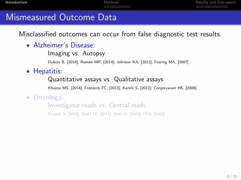
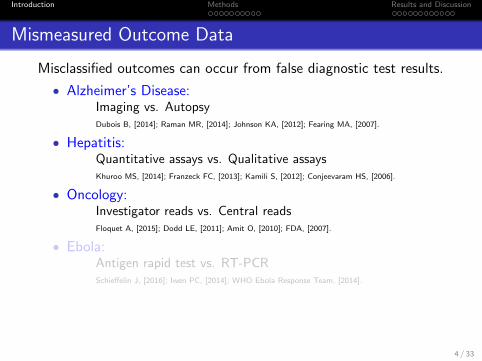
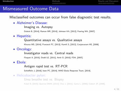
Misclassified outcomes can occur from false diagnostic test results.
● Alzheimer’s Disease:Imaging vs. AutopsyDubois B, [2014]; Raman MR, [2014]; Johnson KA, [2012]; Fearing MA, [2007].
● Hepatitis:Quantitative assays vs. Qualitative assaysKhuroo MS, [2014]; Franzeck FC, [2013]; Kamili S, [2012]; Conjeevaram HS, [2006].
● Oncology:Investigator reads vs. Central readsFloquet A, [2015]; Dodd LE, [2011]; Amit O, [2010]; FDA, [2007].
● Ebola:Antigen rapid test vs. RT-PCRSchieffelin J, [2016]; Iwen PC, [2014]; WHO Ebola Response Team, [2014].
● Helicobacter pylori:Urea breathe test vs. BiopsyKalali B, [2015]; Queiroz DMM, [2013]; Choi J, [2011]; Gatta L, [2006]; Gisbert JP, [2006].
4 / 33
Introduction. . . . . . . . . .Methods
. . . . . . . . . . . .Results and Discussion
Mismeasured Outcome Data
Misclassified outcomes can occur from false diagnostic test results.
● Alzheimer’s Disease:Imaging vs. AutopsyDubois B, [2014]; Raman MR, [2014]; Johnson KA, [2012]; Fearing MA, [2007].
● Hepatitis:Quantitative assays vs. Qualitative assaysKhuroo MS, [2014]; Franzeck FC, [2013]; Kamili S, [2012]; Conjeevaram HS, [2006].
● Oncology:Investigator reads vs. Central readsFloquet A, [2015]; Dodd LE, [2011]; Amit O, [2010]; FDA, [2007].
● Ebola:Antigen rapid test vs. RT-PCRSchieffelin J, [2016]; Iwen PC, [2014]; WHO Ebola Response Team, [2014].
● Helicobacter pylori:Urea breathe test vs. BiopsyKalali B, [2015]; Queiroz DMM, [2013]; Choi J, [2011]; Gatta L, [2006]; Gisbert JP, [2006].
4 / 33
Introduction. . . . . . . . . .Methods
. . . . . . . . . . . .Results and Discussion
Mismeasured Outcome Data
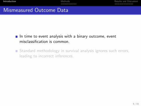
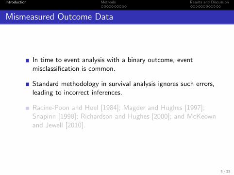
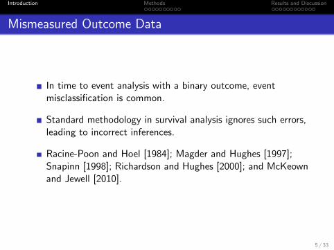
In time to event analysis with a binary outcome, eventmisclassification is common.
Standard methodology in survival analysis ignores such errors,leading to incorrect inferences.
Racine-Poon and Hoel [1984]; Magder and Hughes [1997];Snapinn [1998]; Richardson and Hughes [2000]; and McKeownand Jewell [2010].
5 / 33
Introduction. . . . . . . . . .Methods
. . . . . . . . . . . .Results and Discussion
Mismeasured Outcome Data
In time to event analysis with a binary outcome, eventmisclassification is common.
Standard methodology in survival analysis ignores such errors,leading to incorrect inferences.
Racine-Poon and Hoel [1984]; Magder and Hughes [1997];Snapinn [1998]; Richardson and Hughes [2000]; and McKeownand Jewell [2010].
5 / 33
Introduction. . . . . . . . . .Methods
. . . . . . . . . . . .Results and Discussion
Discrete Time Survival Data
Two Types of Discrete Time
...1 Derived Discrete
...2 Intrinsically Discrete
6 / 33
Introduction. . . . . . . . . .Methods
. . . . . . . . . . . .Results and Discussion
Discrete Time Survival Data
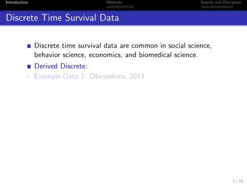
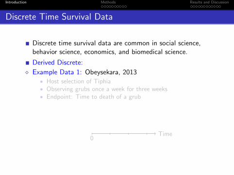
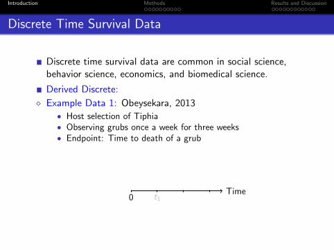
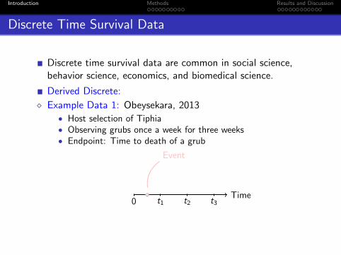
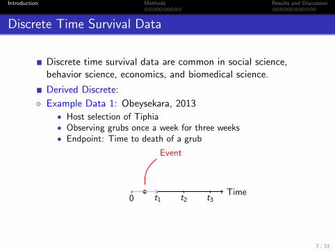
Discrete time survival data are common in social science,behavior science, economics, and biomedical science.
Derived Discrete:
◇ Example Data 1: Obeysekara, 2013
● Host selection of Tiphia● Observing grubs once a week for three weeks● Endpoint: Time to death of a grub
. .Time.0 .t1 .t2 .t3
.
.
.Event
● By grouping, recorded into a discrete time
7 / 33
Introduction. . . . . . . . . .Methods
. . . . . . . . . . . .Results and Discussion
Discrete Time Survival Data
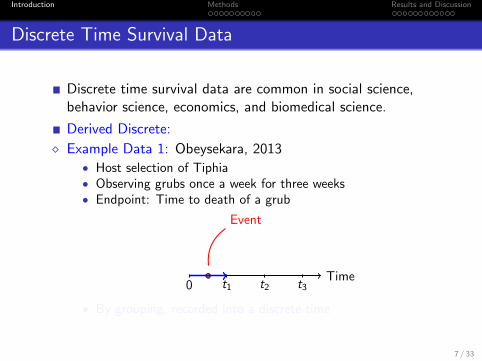
Discrete time survival data are common in social science,behavior science, economics, and biomedical science.
Derived Discrete:
◇ Example Data 1: Obeysekara, 2013
● Host selection of Tiphia● Observing grubs once a week for three weeks● Endpoint: Time to death of a grub
. .Time.0
.t1 .t2 .t3.
.
.Event
● By grouping, recorded into a discrete time
7 / 33
Introduction. . . . . . . . . .Methods
. . . . . . . . . . . .Results and Discussion
Discrete Time Survival Data
Discrete time survival data are common in social science,behavior science, economics, and biomedical science.
Derived Discrete:
◇ Example Data 1: Obeysekara, 2013
● Host selection of Tiphia● Observing grubs once a week for three weeks● Endpoint: Time to death of a grub
. .Time.0 .t1
.t2 .t3.
.
.Event
● By grouping, recorded into a discrete time
7 / 33

Introduction. . . . . . . . . .Methods
. . . . . . . . . . . .Results and Discussion
Discrete Time Survival Data
Discrete time survival data are common in social science,behavior science, economics, and biomedical science.
Derived Discrete:
◇ Example Data 1: Obeysekara, 2013
● Host selection of Tiphia● Observing grubs once a week for three weeks● Endpoint: Time to death of a grub
. .Time.0 .t1 .t2
.t3.
.
.Event
● By grouping, recorded into a discrete time
7 / 33

Introduction. . . . . . . . . .Methods
. . . . . . . . . . . .Results and Discussion
Discrete Time Survival Data
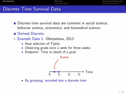
Discrete time survival data are common in social science,behavior science, economics, and biomedical science.
Derived Discrete:
◇ Example Data 1: Obeysekara, 2013
● Host selection of Tiphia● Observing grubs once a week for three weeks● Endpoint: Time to death of a grub
. .Time.0 .t1 .t2 .t3
.
.
.Event
● By grouping, recorded into a discrete time
7 / 33
Introduction. . . . . . . . . .Methods
. . . . . . . . . . . .Results and Discussion
Discrete Time Survival Data
Discrete time survival data are common in social science,behavior science, economics, and biomedical science.
Derived Discrete:
◇ Example Data 1: Obeysekara, 2013
● Host selection of Tiphia● Observing grubs once a week for three weeks● Endpoint: Time to death of a grub
. .Time.0 .t1 .t2 .t3
.
.
.Event
● By grouping, recorded into a discrete time
7 / 33
Introduction. . . . . . . . . .Methods
. . . . . . . . . . . .Results and Discussion
Discrete Time Survival Data
◇ Example Data 2: SEER (Surveillance, Epidemiology, and EndResults) breast cancer data in Joeng et al., 2015.
● Endpoint: Time to death● Unit of survival time: Month - which is rounded due to patient
confidentiality● By rounding, recorded into a discrete time
8 / 33
Introduction. . . . . . . . . .Methods
. . . . . . . . . . . .Results and Discussion
Discrete Time Survival Data
◇ Example Data 2: SEER (Surveillance, Epidemiology, and EndResults) breast cancer data in Joeng et al., 2015.
● Endpoint: Time to death● Unit of survival time: Month - which is rounded due to patient
confidentiality
● By rounding, recorded into a discrete time
8 / 33
Introduction. . . . . . . . . .Methods
. . . . . . . . . . . .Results and Discussion
Discrete Time Survival Data
◇ Example Data 2: SEER (Surveillance, Epidemiology, and EndResults) breast cancer data in Joeng et al., 2015.
● Endpoint: Time to death● Unit of survival time: Month - which is rounded due to patient
confidentiality● By rounding, recorded into a discrete time
8 / 33
Introduction. . . . . . . . . .Methods
. . . . . . . . . . . .Results and Discussion
Discrete Time Survival Data
◇ Example Data 2: SEER (Surveillance, Epidemiology, and EndResults) breast cancer data in Joeng et al., 2015.
● Endpoint: Time to death● Unit of survival time: Month - which is rounded due to patient
confidentiality● By rounding, recorded into a discrete time
8 / 33
Introduction. . . . . . . . . .Methods
. . . . . . . . . . . .Results and Discussion
Discrete Time Survival Data
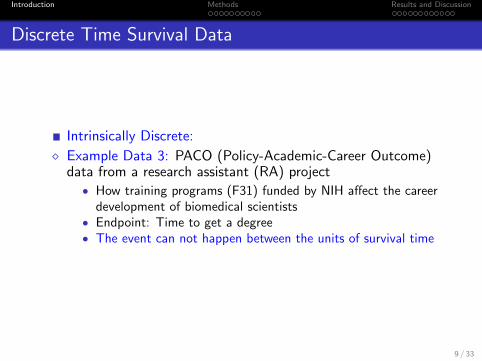
Intrinsically Discrete:
◇ Example Data 3: PACO (Policy-Academic-Career Outcome)data from a research assistant (RA) project
● How training programs (F31) funded by NIH affect the careerdevelopment of biomedical scientists
● Endpoint: Time to get a degree
● The event can not happen between the units of survival time
9 / 33

Introduction. . . . . . . . . .Methods
. . . . . . . . . . . .Results and Discussion
Discrete Time Survival Data
Intrinsically Discrete:
◇ Example Data 3: PACO (Policy-Academic-Career Outcome)data from a research assistant (RA) project
● How training programs (F31) funded by NIH affect the careerdevelopment of biomedical scientists
● Endpoint: Time to get a degree● The event can not happen between the units of survival time
9 / 33

Introduction. . . . . . . . . .Methods
. . . . . . . . . . . .Results and Discussion
Discrete Time Survival Data
◇ Example Data 4: VIRAHEP-C study in Adeniji et al., 2014● Viral resistance to antiviral therapy of chronic Hepatitis C● Endpoint: Time to viral negativity
● The viral loads of HCV (Hepatitis C virus) are measured only at
clinical visits and the event happens only over these visits
● None of the information is available between the unit ofsurvival time.
10 / 33

Outline
.. .1 Introduction
.. .2 Methods
.. .3 Results and Discussion

Introduction. . . . . . . . . .Methods
. . . . . . . . . . . .Results and Discussion
Notations
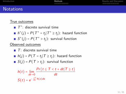
True outcomes
T ∗: discrete survival time
h∗(j) = P(T ∗ = tj ∣T ∗ ≥ tj): hazard function
S∗(j) = P(T ∗ > tj): survival functionObserved outcomes
T : discrete survival time
h(j) = P(T = tj ∣T ≥ tj): hazard function
S(j) = P(T > tj): survival function
h(t) = limdt→0
Pr{t ≤ T < t + dt ∣T ≥ t}dt
S(t) = e− ∫t0 h(s)ds
11 / 33

Introduction. . . . . . . . . .Methods
. . . . . . . . . . . .Results and Discussion
Notations
True outcomes
T ∗: discrete survival time
h∗(j) = P(T ∗ = tj ∣T ∗ ≥ tj): hazard function
S∗(j) = P(T ∗ > tj): survival functionObserved outcomes
T : discrete survival time
h(j) = P(T = tj ∣T ≥ tj): hazard function
S(j) = P(T > tj): survival function
h(t) = limdt→0
Pr{t ≤ T < t + dt ∣T ≥ t}dt
S(t) = e− ∫t0 h(s)ds
11 / 33

Introduction. . . . . . . . . .Methods
. . . . . . . . . . . .Results and Discussion
Proposed Method
Our method uses accuracy of the diagnostic tool to build abridge between the mismeasured outcomes and the trueoutcomes.
12 / 33
Introduction. . . . . . . . . .Methods
. . . . . . . . . . . .Results and Discussion
Why Accuracy?
Gold standard may not be routinely used due to cost or otherreasons.
● Gold standard test for Alzheimer diagnosis: autopsy
13 / 33
Introduction. . . . . . . . . .Methods
. . . . . . . . . . . .Results and Discussion
Why Accuracy?
Gold standard may not be routinely used due to cost or otherreasons.
● Gold standard test for Alzheimer diagnosis: autopsy
13 / 33

Introduction. . . . . . . . . .Methods
. . . . . . . . . . . .Results and Discussion
Why Accuracy?
● Gold standard test for HCV: viral load ≤ 50 IU/ml
● Routine standard test for HCV: viral load ≤ 600 IU/ml
14 / 33

Introduction. . . . . . . . . .Methods
. . . . . . . . . . . .Results and Discussion
Why Accuracy?
● Gold standard test for HCV: viral load ≤ 50 IU/ml
● Routine standard test for HCV: viral load ≤ 600 IU/ml
14 / 33
Introduction. . . . . . . . . .Methods
. . . . . . . . . . . .Results and Discussion
How to Model Accuracy?
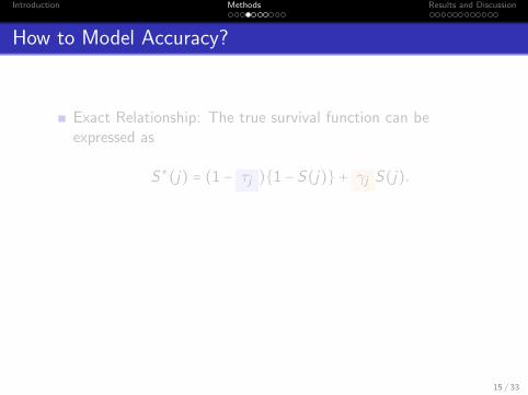
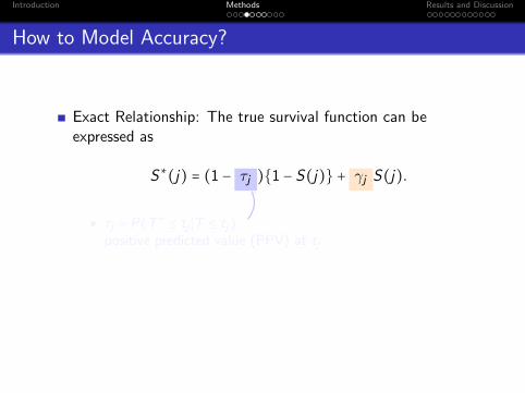
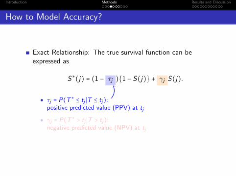
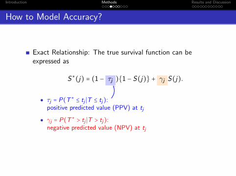
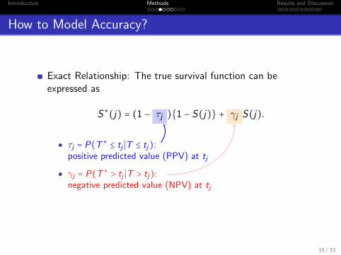
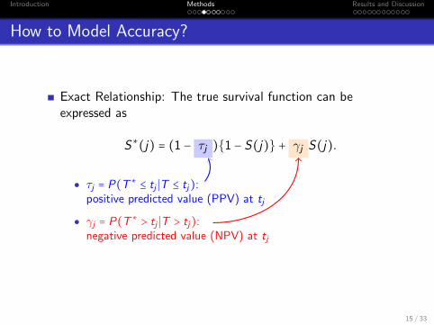
Exact Relationship: The true survival function can beexpressed as
S∗(j) = (1 − ..τj ){1 − S(j)} + ..γj S(j).
● τj = P(T ∗ ≤ tj ∣T ≤ tj): ..positive predicted value (PPV) at tj
● γj = P(T ∗ > tj ∣T > tj): ..
negative predicted value (NPV) at tj
.
15 / 33
Introduction. . . . . . . . . .Methods
. . . . . . . . . . . .Results and Discussion
How to Model Accuracy?
Exact Relationship: The true survival function can beexpressed as
S∗(j) = (1 − ..τj ){1 − S(j)} + ..γj S(j).
● τj = P(T ∗ ≤ tj ∣T ≤ tj): ..positive predicted value (PPV) at tj
● γj = P(T ∗ > tj ∣T > tj): ..
negative predicted value (NPV) at tj
.
15 / 33
Introduction. . . . . . . . . .Methods
. . . . . . . . . . . .Results and Discussion
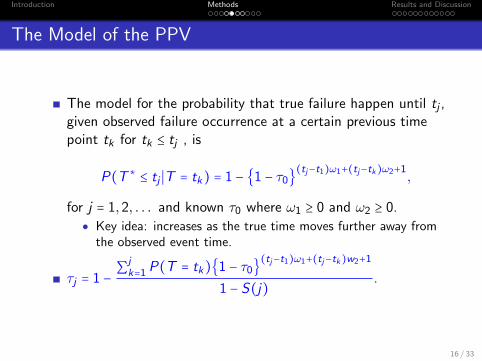
The Model of the PPV
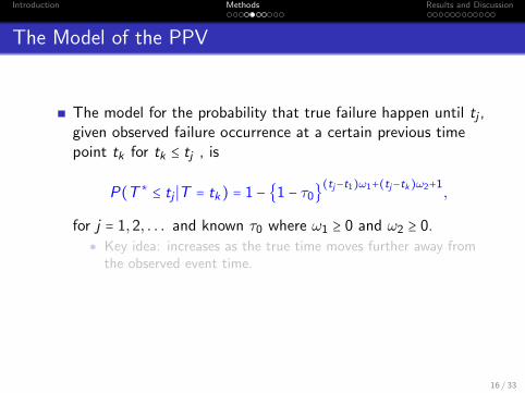
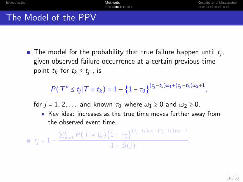
The model for the probability that true failure happen until tj ,given observed failure occurrence at a certain previous timepoint tk for tk ≤ tj , is
P(T ∗ ≤ tj ∣T = tk) = 1 − {1 − τ0}(tj−t1)ω1+(tj−tk)ω2+1
,
for j = 1,2, . . . and known τ0 where ω1 ≥ 0 and ω2 ≥ 0.● Key idea: increases as the true time moves further away from
the observed event time.
τj = 1 −∑j
k=1 P(T = tk){1 − τ0}(tj−t1)ω1+(tj−tk)w2+1
1 − S(j).
16 / 33
Introduction. . . . . . . . . .Methods
. . . . . . . . . . . .Results and Discussion
The Model of the PPV
The model for the probability that true failure happen until tj ,given observed failure occurrence at a certain previous timepoint tk for tk ≤ tj , is
P(T ∗ ≤ tj ∣T = tk) = 1 − {1 − τ0}(tj−t1)ω1+(tj−tk)ω2+1
,
for j = 1,2, . . . and known τ0 where ω1 ≥ 0 and ω2 ≥ 0.● Key idea: increases as the true time moves further away from
the observed event time.
τj = 1 −∑j
k=1 P(T = tk){1 − τ0}(tj−t1)ω1+(tj−tk)w2+1
1 − S(j).
16 / 33
Introduction. . . . . . . . . .Methods
. . . . . . . . . . . .Results and Discussion
Assumption 1
Assumption 1: P(T ∗ ≥ T ) = 1
The “Truth” cannot happen before the “Observed”
17 / 33
Introduction. . . . . . . . . .Methods
. . . . . . . . . . . .Results and Discussion
Assumption 1
Assumption 1: P(T ∗ ≥ T ) = 1
The “Truth” cannot happen before the “Observed”
17 / 33
Introduction. . . . . . . . . .Methods
. . . . . . . . . . . .Results and Discussion
Assumption 1
Assumption 1: P(T ∗ ≥ T ) = 1
The “Truth” cannot happen before the “Observed”
17 / 33
Introduction. . . . . . . . . .Methods
. . . . . . . . . . . .Results and Discussion
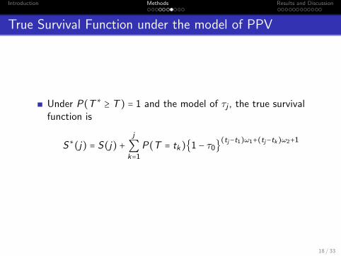
True Survival Function under the model of PPV
Under P(T ∗ ≥ T ) = 1 and the model of τj , the true survivalfunction is
S∗(j) = S(j) +j
∑k=1
P(T = tk){1 − τ0}(tj−t1)ω1+(tj−tk)ω2+1
18 / 33

Introduction. . . . . . . . . .Methods
. . . . . . . . . . . .Results and Discussion
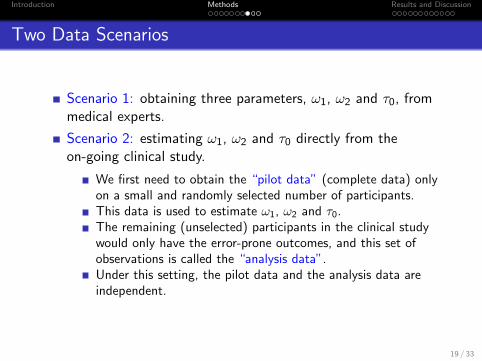
Two Data Scenarios
Scenario 1: obtaining three parameters, ω1, ω2 and τ0, frommedical experts.
Scenario 2: estimating ω1, ω2 and τ0 directly from theon-going clinical study.
We first need to obtain the “pilot data” (complete data) onlyon a small and randomly selected number of participants.This data is used to estimate ω1, ω2 and τ0.The remaining (unselected) participants in the clinical studywould only have the error-prone outcomes, and this set ofobservations is called the “analysis data”.Under this setting, the pilot data and the analysis data areindependent.
19 / 33
Introduction. . . . . . . . . .Methods
. . . . . . . . . . . .Results and Discussion
Two Data Scenarios
Scenario 1: obtaining three parameters, ω1, ω2 and τ0, frommedical experts.
Scenario 2: estimating ω1, ω2 and τ0 directly from theon-going clinical study.
We first need to obtain the “pilot data” (complete data) onlyon a small and randomly selected number of participants.This data is used to estimate ω1, ω2 and τ0.The remaining (unselected) participants in the clinical studywould only have the error-prone outcomes, and this set ofobservations is called the “analysis data”.Under this setting, the pilot data and the analysis data areindependent.
19 / 33

Introduction. . . . . . . . . .Methods
. . . . . . . . . . . .Results and Discussion
Framework of the approximation process
20 / 33

Introduction. . . . . . . . . .Methods
. . . . . . . . . . . .Results and Discussion
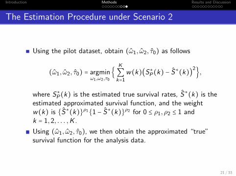
The Estimation Procedure under Scenario 2
Using the pilot dataset, obtain (ω1, ω2, τ0) as follows
(ω1, ω2, τ0) = argminω1,ω2,τ0
{K
∑k=1
w(k)(S∗P(k) − S∗(k))2},
where S∗P(k) is the estimated true survival rates, S∗(k) is theestimated approximated survival function, and the weightw(k) is {S∗(k)}ρ1{1 − S∗(k)}ρ2 for 0 ≤ ρ1, ρ2 ≤ 1 andk = 1,2, . . . ,K .
Using (ω1, ω2, τ0), we then obtain the approximated “true”survival function for the analysis data.
21 / 33
Introduction. . . . . . . . . .Methods
. . . . . . . . . . . .Results and Discussion
The Estimation Procedure under Scenario 2
Using the pilot dataset, obtain (ω1, ω2, τ0) as follows
(ω1, ω2, τ0) = argminω1,ω2,τ0
{K
∑k=1
w(k)(S∗P(k) − S∗(k))2},
where S∗P(k) is the estimated true survival rates, S∗(k) is theestimated approximated survival function, and the weightw(k) is {S∗(k)}ρ1{1 − S∗(k)}ρ2 for 0 ≤ ρ1, ρ2 ≤ 1 andk = 1,2, . . . ,K .
Using (ω1, ω2, τ0), we then obtain the approximated “true”survival function for the analysis data.
21 / 33

Outline
.. .1 Introduction
.. .2 Methods
.. .3 Results and Discussion
Introduction. . . . . . . . . .Methods
. . . . . . . . . . . .Results and Discussion
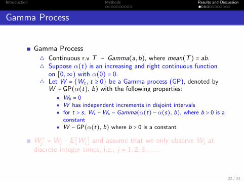
Gamma Process
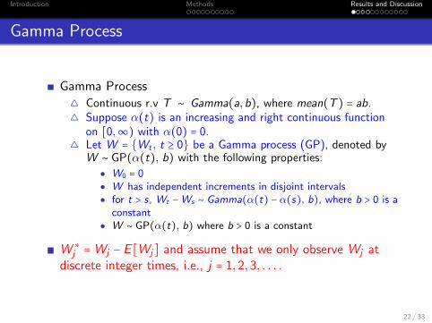
Gamma Process
△ Continuous r.v T ∼ Gamma(a,b), where mean(T ) = ab.△ Suppose α(t) is an increasing and right continuous function
on [0,∞) with α(0) = 0.△ Let W = {Wt , t ≥ 0} be a Gamma process (GP), denoted by
W ∼ GP(α(t), b) with the following properties:
● W0 = 0● W has independent increments in disjoint intervals● for t > s, Wt −Ws ∼ Gamma(α(t) − α(s), b), where b > 0 is a
constant● W ∼ GP(α(t), b) where b > 0 is a constant
W ∗j =Wj − E [Wj] and assume that we only observe Wj at
discrete integer times, i.e., j = 1,2,3, . . . .
22 / 33
Introduction. . . . . . . . . .Methods
. . . . . . . . . . . .Results and Discussion
Gamma Process
Gamma Process
△ Continuous r.v T ∼ Gamma(a,b), where mean(T ) = ab.△ Suppose α(t) is an increasing and right continuous function
on [0,∞) with α(0) = 0.△ Let W = {Wt , t ≥ 0} be a Gamma process (GP), denoted by
W ∼ GP(α(t), b) with the following properties:
● W0 = 0● W has independent increments in disjoint intervals● for t > s, Wt −Ws ∼ Gamma(α(t) − α(s), b), where b > 0 is a
constant● W ∼ GP(α(t), b) where b > 0 is a constant
W ∗j =Wj − E [Wj] and assume that we only observe Wj at
discrete integer times, i.e., j = 1,2,3, . . . .
22 / 33
Introduction. . . . . . . . . .Methods
. . . . . . . . . . . .Results and Discussion
Survival function with a lower detection level underGamma Process
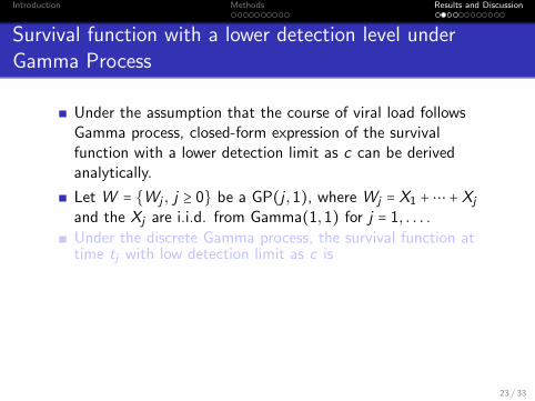
Under the assumption that the course of viral load followsGamma process, closed-form expression of the survivalfunction with a lower detection limit as c can be derivedanalytically.
Let W = {Wj , j ≥ 0} be a GP(j ,1), where Wj = X1 +⋯ +Xj
and the Xj are i.i.d. from Gamma(1,1) for j = 1, . . . .Under the discrete Gamma process, the survival function attime tj with low detection limit as c is
Sc(j) = P(X1 ≥ 1 + c,X1 +X2 ≥ 2 + c, . . . ,X1 +⋯ +Xj ≥ n + c)
= j(j−1)
(j − 1)!exp{−(c + j)}.
23 / 33
Introduction. . . . . . . . . .Methods
. . . . . . . . . . . .Results and Discussion
Survival function with a lower detection level underGamma Process
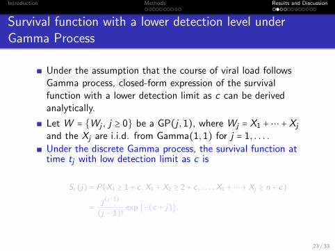
Under the assumption that the course of viral load followsGamma process, closed-form expression of the survivalfunction with a lower detection limit as c can be derivedanalytically.
Let W = {Wj , j ≥ 0} be a GP(j ,1), where Wj = X1 +⋯ +Xj
and the Xj are i.i.d. from Gamma(1,1) for j = 1, . . . .Under the discrete Gamma process, the survival function attime tj with low detection limit as c is
Sc(j) = P(X1 ≥ 1 + c,X1 +X2 ≥ 2 + c, . . . ,X1 +⋯ +Xj ≥ n + c)
= j(j−1)
(j − 1)!exp{−(c + j)}.
23 / 33
Introduction. . . . . . . . . .Methods
. . . . . . . . . . . .Results and Discussion
Survival function with a lower detection level underGamma Process
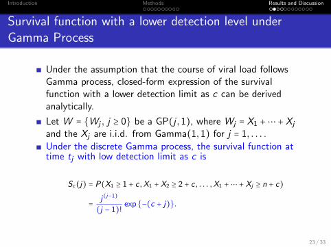
Under the assumption that the course of viral load followsGamma process, closed-form expression of the survivalfunction with a lower detection limit as c can be derivedanalytically.
Let W = {Wj , j ≥ 0} be a GP(j ,1), where Wj = X1 +⋯ +Xj
and the Xj are i.i.d. from Gamma(1,1) for j = 1, . . . .Under the discrete Gamma process, the survival function attime tj with low detection limit as c is
Sc(j) = P(X1 ≥ 1 + c,X1 +X2 ≥ 2 + c, . . . ,X1 +⋯ +Xj ≥ n + c)
= j(j−1)
(j − 1)!exp{−(c + j)}.
23 / 33

Introduction. . . . . . . . . .Methods
. . . . . . . . . . . .Results and Discussion
Survival Functions Under Gamma Process with c∗ = −0.8and c = −0.4
True survival function:
Sc∗(j) =j(j−1)
(j − 1)!exp{−(c∗ + j)}.
Observed survival function:
Sc(j) =j(j−1)
(j − 1)!exp{−(c + j)}.
Approximated survival function: S∗c (j).
24 / 33
Introduction. . . . . . . . . .Methods
. . . . . . . . . . . .Results and Discussion
Survival functions with c∗ = −0.8, c = −0.4 for ρ1 = ρ2 = 0.5
If c∗ ≤ c then P(T ∗ ≥ T ) = 1.
25 / 33

Introduction. . . . . . . . . .Methods
. . . . . . . . . . . .Results and Discussion
Brownian Motion(BM) Process
Let W = {Wt , t ≥ 0} be a standard BM process satisfying thefollowing properties:
△ W0 = 0.△ W (tk) −W (ts) ∼ N(0,
tk − ts60000
), for 0 ≤ ts < tk ≤ tK .△ Wt1 ,Wt2 −Wt1 , . . . ,Wtk −Wts are independent.△ Wk ∼ N(0, k).
26 / 33

Introduction. . . . . . . . . .Methods
. . . . . . . . . . . .Results and Discussion
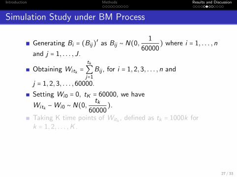
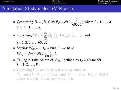
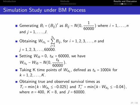
Simulation Study under BM Process
Generating Bi = (Bij)′ as Bij ∼ N(0,1
60000) where i = 1, . . . ,n
and j = 1, . . . , J.
Obtaining Wi tk =tk
∑j=1
Bij , for i = 1,2,3, . . . ,n and
j = 1,2,3, . . . ,60000.Setting Wi0 = 0, tK = 60000, we have
Wi tk −Wi0 ∼ N(0,tk
60000).
Taking K time points of Witk , defined as tk = 1000k fork = 1,2, . . . ,K .
Obtaining true and observed survival times asTi = min{k ∶Witk ≤ −0.025} and T ∗i = min{k ∶Witk ≤ −0.04},where n = 400, K = 8, and J = 60000.
27 / 33
Introduction. . . . . . . . . .Methods
. . . . . . . . . . . .Results and Discussion
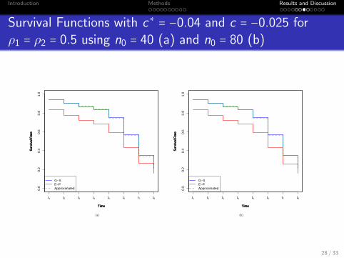
Survival Functions with c∗ = −0.04 and c = −0.025 forρ1 = ρ2 = 0.5 using n0 = 40 (a) and n0 = 80 (b)
Time
Sur
viva
l Rat
e
Time
Sur
viva
l Rat
e
Time
Sur
viva
l Rat
e
t1 t2 t3 t4 t5 t6 t7 t8
0.0
0.2
0.4
0.6
0.8
1.0
G−SE−PApproximated
Time
Sur
viva
l Rat
e
Time
Sur
viva
l Rat
e
Time
Sur
viva
l Rat
e
t1 t2 t3 t4 t5 t6 t7 t8
0.0
0.2
0.4
0.6
0.8
1.0
G−SE−PApproximated
(a) (b)
28 / 33
Introduction. . . . . . . . . .Methods
. . . . . . . . . . . .Results and Discussion
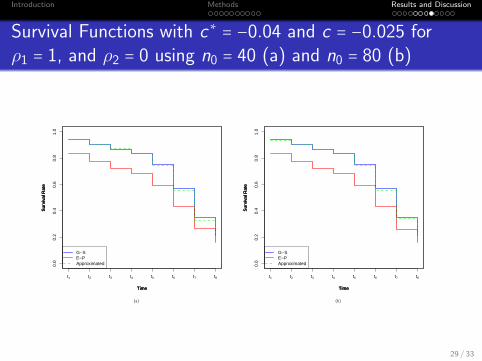
Survival Functions with c∗ = −0.04 and c = −0.025 forρ1 = 1, and ρ2 = 0 using n0 = 40 (a) and n0 = 80 (b)
Time
Sur
viva
l Rat
e
Time
Sur
viva
l Rat
e
Time
Sur
viva
l Rat
e
t1 t2 t3 t4 t5 t6 t7 t8
0.0
0.2
0.4
0.6
0.8
1.0
G−SE−PApproximated
Time
Sur
viva
l Rat
e
Time
Sur
viva
l Rat
e
Time
Sur
viva
l Rat
e
t1 t2 t3 t4 t5 t6 t7 t8
0.0
0.2
0.4
0.6
0.8
1.0
G−SE−PApproximated
(a) (b)
29 / 33
Introduction. . . . . . . . . .Methods
. . . . . . . . . . . .Results and Discussion
Data
372 subjects from the VIRAHEP-C (Viral Resistance toAntiviral Therapy of Chronic Hepatitis C) Study
True event at time tj :
E∗j = I{ viral load ≤ 50 IU/ml at tj}
Observed event at time tj :
Ej = I{ viral load ≤ 600 IU/ml at tj}
30 / 33
Introduction. . . . . . . . . .Methods
. . . . . . . . . . . .Results and Discussion
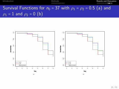
Survival Functions for n0 = 37 with ρ1 = ρ2 = 0.5 (a) andρ1 = 1 and ρ2 = 0 (b)
Time
Sur
viva
l Rat
e
Time
Sur
viva
l Rat
e
Time
Sur
viva
l Rat
e
t1 t2 t3 t4 t5 t6 t7 t8
0.0
0.2
0.4
0.6
0.8
1.0
G−SE−PApproximated
Time
Sur
viva
l Rat
e
Time
Sur
viva
l Rat
e
Time
Sur
viva
l Rat
e
t1 t2 t3 t4 t5 t6 t7 t8
0.0
0.2
0.4
0.6
0.8
1.0
G−SE−PApproximated
(a) (b)
31 / 33
Introduction. . . . . . . . . .Methods
. . . . . . . . . . . .Results and Discussion
Concluding Remarks
Our discrete-time survival estimator:...1 allows for the cumulative probability of correctly classifying a G-S event
to increase with time given the prior occurrence of an E-P event,
...2 allows for the inclusion of estimated model parameters D1 = (ω1, ω2, τ0)through a validation subsample (“pilot dataset”).
32 / 33

Introduction. . . . . . . . . .Methods
. . . . . . . . . . . .Results and Discussion
Thank You!
We offer a more flexible strategy to the conduct of clinical trials,there is a possibility to reduce cost and improve efficiency.
33 / 33