Image Registration with Homography: A Refresherwith Differentiable Mutual Information, Ordinary

Differential Equation and Complex Matrix Exponential

by

Abhishek Nan

A thesis submitted in partial fulfillment of the requirements for the degree of

Master of Science

Department of Computing Science

University of Alberta

c© Abhishek Nan, 2020

Abstract

This work presents a novel method of tackling the task of image registration.

Our algorithm uses a differentiable form of Mutual Information implemented

via a neural network called MINE. An important property of neural networks is

them being differentiable, which allows them to be used as a loss function. This

way we use MINE as an estimator for our loss function. Furthermore to make

the optimization smoother, we parametrize the transformation module using

complex matrix manifolds which further improves our accuracy and efficiency.

In order to speed up computation and make the algorithm more robust we use

a multi-resolution approach, but implement it as a simultaneous loss from all

levels, which provides the aforementioned benefits. The parameters for each

resolution are modelled via ordinary differential equations and solved using a

neural network which adds to the final performance scores as well. This leads

to a state of the art algorithm implemented via modern software frameworks

which allow for automatic gradient computations (such as PyTorch). Our

algorithm performs better than registration algorithms available off the shelf

in state of the art image registration tools/softwares. We demonstrate this on

four open source datasets. The source code is publicly available on Github1.

1Link to source code: https://github.com/abnan/ODECME

ii

Preface

This is a collaborative work with Dr. Nilanjan Ray and Dr. Matthew Tennant.

Parts of this thesis have been submitted to Medical Imaging with Deep Learn-

ing (MIDL 2020) and IEEE Transactions on Medical Imaging (IEEE TMI).

These submissions were co-authored with Dr. Nilanjan Ray, Dr. Matthew

Tennant and Dr. Uriel Rubin.

iii

To my parents

For being a constant source of inspiration.

iv

I could either watch it happen or be a part of it.

– Elon Reeve Musk, 2019.

v

Acknowledgements

I would like to thank Dr. Nilanjan Ray. His guidance throughout the period

of my program made this work possible. I owe a debt of gratitude to my

parents who supported my decision to move away far from home in pursuit

of furthering my education. They have been a source of constant inspiration

and strength throughout. Last, but not least, I would also like to express my

gratitude to Dr. Matt Tennant for his continued support.

This work was supported in part by NSERC Discovery Grants.

vi

Contents

1 Introduction 11.1 Problem definition . . . . . . . . . . . . . . . . . . . . . . . . 11.2 Significance of problem . . . . . . . . . . . . . . . . . . . . . . 31.3 Motivation . . . . . . . . . . . . . . . . . . . . . . . . . . . . . 41.4 Thesis contribution . . . . . . . . . . . . . . . . . . . . . . . . 51.5 Organization of the Thesis . . . . . . . . . . . . . . . . . . . . 7

2 Background 92.1 Optimization for Image Registration . . . . . . . . . . . . . . 9

2.1.1 Mean Square Error . . . . . . . . . . . . . . . . . . . . 92.1.2 Mutual Information . . . . . . . . . . . . . . . . . . . . 102.1.3 Mutual Information Neural Estimation . . . . . . . . . 14

2.2 Multi-resolution Computation . . . . . . . . . . . . . . . . . . 152.3 Matrix Exponential . . . . . . . . . . . . . . . . . . . . . . . . 182.4 Ordinary Differential Equations . . . . . . . . . . . . . . . . . 20

3 Related Works 233.1 Feature based approaches . . . . . . . . . . . . . . . . . . . . 233.2 Learning based approaches . . . . . . . . . . . . . . . . . . . . 253.3 Optimization based approaches . . . . . . . . . . . . . . . . . 26

4 Proposed Multi-Resolution Image Registration 294.1 Differentiable Mutual Information and Matrix Exponential for

Multi-Resolution Image Registration . . . . . . . . . . . . . . 294.1.1 MINE for images . . . . . . . . . . . . . . . . . . . . . 294.1.2 DRMIME Algorithm . . . . . . . . . . . . . . . . . . . 31

4.2 Ordinary Differential Equation and Complex Matrix Exponen-tial for Multi-resolution Image Registration . . . . . . . . . . . 334.2.1 ODE for Multi-resolution Image Registration . . . . . . 334.2.2 Symmetric loss function . . . . . . . . . . . . . . . . . 344.2.3 Complex Matrix Exponential . . . . . . . . . . . . . . 354.2.4 ODECME Algorithm . . . . . . . . . . . . . . . . . . . 36

5 Experiments 395.1 Datasets . . . . . . . . . . . . . . . . . . . . . . . . . . . . . . 39

5.1.1 FIRE . . . . . . . . . . . . . . . . . . . . . . . . . . . . 395.1.2 ANHIR . . . . . . . . . . . . . . . . . . . . . . . . . . 415.1.3 IXI . . . . . . . . . . . . . . . . . . . . . . . . . . . . . 425.1.4 ADNI . . . . . . . . . . . . . . . . . . . . . . . . . . . 43

5.2 Competing algorithms . . . . . . . . . . . . . . . . . . . . . . 435.3 Results . . . . . . . . . . . . . . . . . . . . . . . . . . . . . . . 455.4 Ablation study . . . . . . . . . . . . . . . . . . . . . . . . . . 54

5.4.1 Effect of multi-resolution . . . . . . . . . . . . . . . . . 54

vii

5.4.2 Effect of matrix exponentiation . . . . . . . . . . . . . 555.4.3 Effect of Sampling strategy . . . . . . . . . . . . . . . 555.4.4 Effect of CME . . . . . . . . . . . . . . . . . . . . . . . 565.4.5 Effect of ODE . . . . . . . . . . . . . . . . . . . . . . . 57

5.5 Efficiency . . . . . . . . . . . . . . . . . . . . . . . . . . . . . 58

6 Conclusion 62

References 63

Appendix A 71A.1 DV Lower Bound Reaches Mutual Information . . . . . . . . . 71A.2 Algorithm Hyperparameters . . . . . . . . . . . . . . . . . . . 72

A.2.1 DRMIME . . . . . . . . . . . . . . . . . . . . . . . . . 72A.2.2 ODECME . . . . . . . . . . . . . . . . . . . . . . . . . 72A.2.3 MMI . . . . . . . . . . . . . . . . . . . . . . . . . . . . 73A.2.4 JHMI . . . . . . . . . . . . . . . . . . . . . . . . . . . 73A.2.5 MSE . . . . . . . . . . . . . . . . . . . . . . . . . . . . 74A.2.6 NCC . . . . . . . . . . . . . . . . . . . . . . . . . . . . 74A.2.7 NMI . . . . . . . . . . . . . . . . . . . . . . . . . . . . 74A.2.8 AMI . . . . . . . . . . . . . . . . . . . . . . . . . . . . 74

viii

List of Tables

5.1 NAED for FIRE dataset along with paired t-test significancevalues . . . . . . . . . . . . . . . . . . . . . . . . . . . . . . . 46

5.2 NAED for ANHIR dataset along with paired t-test significancevalues . . . . . . . . . . . . . . . . . . . . . . . . . . . . . . . 48

5.3 SSIM for IXI dataset along with paired t-test significance values 515.4 PSNR for IXI dataset along with paired t-test significance values 525.5 MSE for IXI dataset along with paired t-test significance values 525.6 SSIM for ADNI dataset along with paired t-test significance values 535.7 PSNR for ADNI dataset along with paired t-test significance

values . . . . . . . . . . . . . . . . . . . . . . . . . . . . . . . 535.8 NAED for DRMIME with and without using multi-resolution

pyramids. P-value is from paired t-test between both cases. . . 545.9 NAED for MINE with and without using manifolds. P-value is

from paired t-test between both cases. . . . . . . . . . . . . . 555.10 NAED for DRMIME with Canny edge detection and Random

Sampling (10%). P-value is from paired t-test between both cases. 565.11 The average range and standard deviation of real and imaginary

coefficients after registering the FIRE dataset . . . . . . . . . 585.12 Time taken for 1000 epochs and resultant NAED (lower is better) 59

ix

List of Figures

1.1 A pair of images from the FIRE dataset with the ground truthdepicted as white spots. . . . . . . . . . . . . . . . . . . . . . 2

1.2 A pair of images from the FIRE dataset . . . . . . . . . . . . 2

2.1 Example of joint histogram involved in MI computation formulti-modal images. The image on the left is a CT scan andthe middle is a MR scan. The image on the right is a jointhistogram with the grey values of the CT scan on the x-axisand the MR scan on the y-axis. For each (x,y) co-ordinate inthe histogram, if they are corresponding points from the CTimage and MR image respectively, the intensity at point (x,y)is increased. Source: Pluim, Maintz, and Viergever [57] . . . . 11

2.2 Joint histogram of an image with itself. (Source: Pluim, Maintz,and Viergever [59]) The leftmost is the unchanged image withitself and as we go right, it depicts the joint histogram of theimage with a version of it that has been rotated by angles of2, 5 and 10 degree respectively. Below the histograms are thejoint entropy values. . . . . . . . . . . . . . . . . . . . . . . . 13

2.3 MINE as proposed by Belghazi et al. in [8] . . . . . . . . . . . 152.4 Multi-resolution pyramid (Source: Wikipedia) . . . . . . . . . 16

3.1 Example of feature matching. Source: https://www.sicara.ai/blog/2019-07-16-image-registration-deep-learning . . . . . . . . . . . . . 24

3.2 Structure of HomographyNet as proposed by DeTone, Malisiewicz,and Rabinovich [18] . . . . . . . . . . . . . . . . . . . . . . . . 26

4.1 Given a pair of images, MINE converges to the DV lower bound. 304.2 Pipeline for the DRMIME Registration algorithm . . . . . . . 324.3 Randomly generated grids by complex matrix exponential (4.10)

and complex transformation (4.11). Elements of Br were gen-erated by a zero mean Gaussian with 0.1 standard deviation(SD) for all four panels. Elements of Bi were generated by azero mean Gaussian with SD as follows: 0 for top-left, 0.1 fortop-right, 0.2 for bottom-left and 0.3 for bottom-right panel. . 36

4.4 Pipeline for the ODECME Registration algorithm (using multi-resolution pyramid of 3 levels) . . . . . . . . . . . . . . . . . . 37

5.1 Pairs in each column belong to the same category. Column cat-egories from left to right: S, P, A, A. White dots indicate controlpoint locations. Source: https://projects.ics.forth.gr/cvrl/fire/ 40

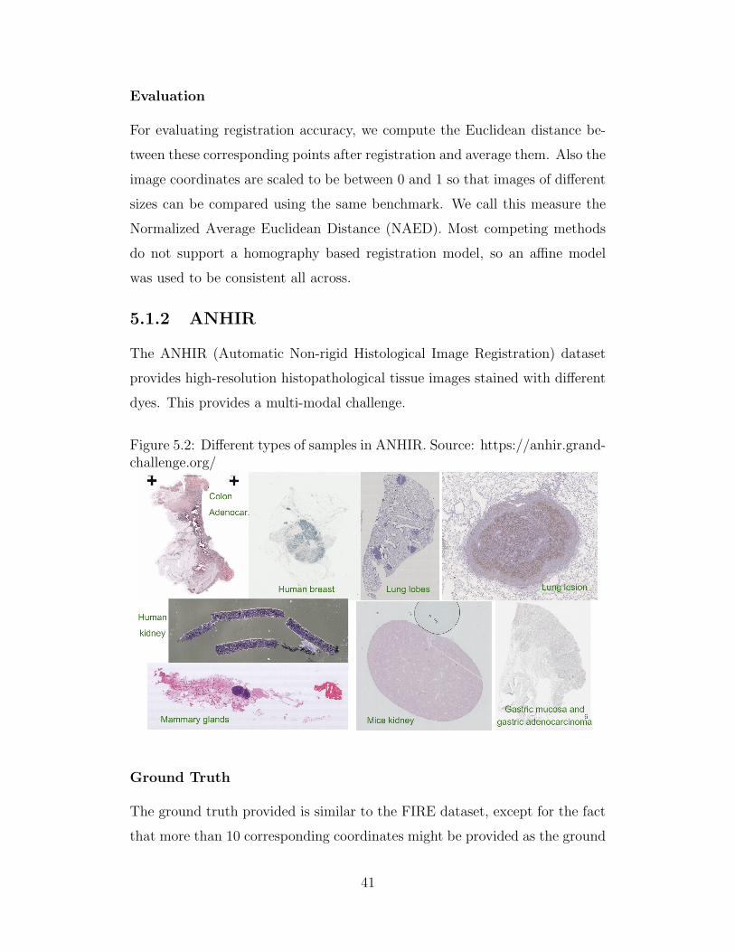
5.2 Different types of samples in ANHIR. Source: https://anhir.grand-challenge.org/ . . . . . . . . . . . . . . . . . . . . . . . . . . . 41

x

5.3 The images on the left show a pair to be registered from theFIRE dataset. The images on the right represent the differencebetween the transformed moving image and the fixed imageafter registration by different algorithms. Source: Nan et al. [54] 46

5.4 Box plot for NAED of the best 5 performing algorithms onFIRE. ODECME refers to ODE (RK4-Complex). . . . . . . . 47

5.5 The images on the left show a pair to be registered from theANHIR dataset. The images on the right represent the dif-ference between the transformed moving image and the fixedimage after registration by different algorithms. . . . . . . . . 48

5.6 Box plot for top 5 performing algorithms on ANHIR. ODECMErefers to ODE (RK4-Complex). . . . . . . . . . . . . . . . . . 49

5.7 Box plot for SSIM values (higher is better) for each algorithmon the IXI datset after registration. ODECME refers to ODE(RK4-Complex). . . . . . . . . . . . . . . . . . . . . . . . . . 49

5.8 Box plot for PSNR values (higher is better) for each algorithmon the IXI datset after registration. ODECME refers to ODE(RK4-Complex). . . . . . . . . . . . . . . . . . . . . . . . . . 50

5.9 Box plot for MSE values (lower is better) for each algorithmon the IXI datset after registration. ODECME refers to ODE(RK4-Complex). . . . . . . . . . . . . . . . . . . . . . . . . . 50

5.10 The images on the left show the middle slice of a pair of volumesto be registered from the IXI dataset. The images on the rightrepresent the difference between the middle slices of the trans-formed moving volume and the fixed volume after registrationby different algorithms. . . . . . . . . . . . . . . . . . . . . . . 51

5.11 Box plot for SSIM values (higher is better) for each algorithmon the ADNI dataset after registration. ODECME refers toODE (RK4-Complex). . . . . . . . . . . . . . . . . . . . . . . 52

5.12 Box plot for PSNR values (higher is better) for each algorithmon the ADNI dataset after registration. ODECME refers toODE (RK4-Complex). . . . . . . . . . . . . . . . . . . . . . . 53

5.16 NAED averaged for 10 randomly selected pairs from FIRE, plot-ted over 500 epochs. The error bars represent the standarddeviation. . . . . . . . . . . . . . . . . . . . . . . . . . . . . . 57

5.17 Plot showing how individual coefficients generated by ODEnetvary with successive resolution levels. Level 0 is the originalimage and 4 denotes the coarsest resolution. . . . . . . . . . . 58

5.13 Randomly selected slices from the difference volume before reg-istration between the reference and a randomly moving volumefrom the ADNI dataset. Each row represents slices from a dif-ferent axis. . . . . . . . . . . . . . . . . . . . . . . . . . . . . . 61

5.14 Same slices from the difference volume after registration usingODECME. . . . . . . . . . . . . . . . . . . . . . . . . . . . . . 61

5.15 Same slices from the difference volume after registration usingMSE. . . . . . . . . . . . . . . . . . . . . . . . . . . . . . . . . 61

xi

Chapter 1

Introduction

1.1 Problem definition

Image registration is the task of finding the correspondences across two or

more images and bringing the images into a single coordinate system. This is

often used to tackle problems in the field of medical imaging, remote sensing,

etc. For instance, in case we want to analyse how the anatomy of a patient’s

body part changes over time, we need snapshots of it over time. Not only could

the source camera change, the location, orientation of the camera as well as of

the patient are variables that could change over time. In such scenarios, doing

a comprehensive analysis becomes difficult and hence, registration becomes a

prerequisite before any further analysis can be done. For instance, Figure 1.1

shows two images from the FIRE (Fundus Image Registration Dataset)[31]

dataset. They are snapshots of the same patient’s retinal fundus taken few

months apart. The white spots show corresponding anatomical points which

should ideally be completely overlapping, but aren’t due to changes over time.

Hence, they need to be registered before further analysis. In this thesis, we

tackle this problem of pairwise registration, where we try to find the points of

correspondence between such a pair of images.

1

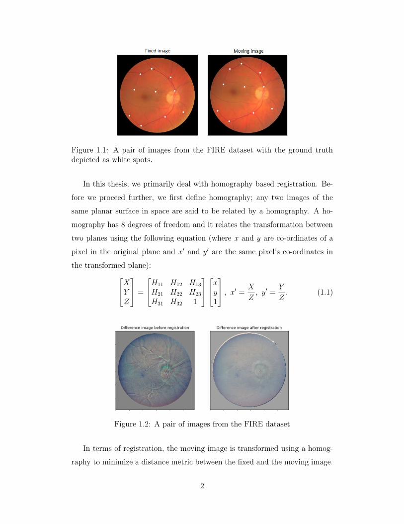
Figure 1.1: A pair of images from the FIRE dataset with the ground truthdepicted as white spots.

In this thesis, we primarily deal with homography based registration. Be-

fore we proceed further, we first define homography; any two images of the

same planar surface in space are said to be related by a homography. A ho-

mography has 8 degrees of freedom and it relates the transformation between

two planes using the following equation (where x and y are co-ordinates of a

pixel in the original plane and x′ and y′ are the same pixel’s co-ordinates in

the transformed plane):XYZ

=

H11 H12 H13

H21 H22 H23

H31 H32 1

xy1

, x′ = X

Z, y′ =

Y

Z. (1.1)

Figure 1.2: A pair of images from the FIRE dataset

In terms of registration, the moving image is transformed using a homog-

raphy to minimize a distance metric between the fixed and the moving image.

2

For instance, in Fig. 1.1 we transform the moving image using the homog-

raphy

1.00 6.64 −0.01−0.06 1.00 6.812.55 −3.7e− 06 1

and Fig. 1.2 shows the difference image

between the fixed image and the moving image before and after the homogra-

phy transformation is applied.

While there are multiple approaches to image registration, they may be

broadly classified into two families based on how the registration parameters

are obtained: learning based and optimization based. While the benefit of

learning based approaches is that once trained on a dataset, inference is quite

fast. On the other hand, the drawback of learning based approaches is that

they need large amounts of training data to achieve satisfactory results and

furthermore, they won’t perform well on pairs which are drastically different

from the training set. Hence, here we try to present an optimization based

approach using which inference might be slightly longer than learning based

methods, but they are very robust and work on any image sets and do not

require annotated training data at all.

1.2 Significance of problem

In the field of fundoscopy, microvascular circulation is observed to diagnose and

monitor diseases such as diabetes and hypertension[29]. For accurate observa-

tions, image registration is a necessary prerequisite. Also due to progression

or remission of retinopathy, there might be structural changes in the retina.

In such a case where images from the same camera source are registered, it is

called mono-modal registration. Once image registration has been performed,

the images can subsequently be used for super-resolution, mosaicing and lon-

gitudinal studies.

Furthermore, the camera source need not always be the same. Different

imaging modalities can provide different and additive information for the clin-

ician or researcher regarding human tissue. For example, radiation of different

wavelengths are able to penetrate human tissues to differing depths. A par-

ticular wavelength might be used to produce a map of bone structure, while

3

a different wavelength could be used to map other internal organs. These

two different maps are referred to as different modalities. A common way

to perform a holistic analysis is to combine the (complimentary) information

from these different modalities. Alignment of the different modalities requires

multi-modal registration. But registering such cross-modal images requires

techniques quite different from mono-modal registration.

In general, the problem of registration is not just limited to the domain

of medical imaging, but is quite pervasive in many domains of digital image

processing. For instance, in the robotics community it is framed as the problem

of template matching, where the objective is to find an object in different

scenes. This could be used for tasks such as object localization [25, 21] or

object tracking [14].

Furthermore, to tackle the problem of image registration, often the model

used to parametrize the registration parameters are fashioned in a hierarchical

manner; i.e. first a global transformation using homography (or its subsets) is

used to register the images as much as possible before applying more elaborate

techniques such as deformable registration. Thus, the success of deformable

registration methods is highly dependent on how successful the initial registra-

tion step was. Our optimization based registration approach tries to improve

this initial global homography based registration.

1.3 Motivation

One of the most successful metrics used for cross-modal or multi-modal medical

image registration is mutual information (MI) [57]. In the context of scalar-

valued images, these joint probabilities are calculated using a two-dimensional

histogram of the two images. Most current MI-based techniques for registra-

tion use slight variations of the above method to approximate MI. While this

works well, there are some issues associated with this method of evaluation as

follows.

• The number of histogram bins chosen becomes a hyperparamter. While

increasing the number of bins would lead to better accuracy in computa-

4

tion, this comes at the cost of time. Furthermore, there is no theoretical

upper bound on the number of bins that should be used for accurate

results.

• Images with higher dimensions (color images, hyper-spectral images),

would need a higher dimensional histograms and a joint histogram re-

quiring a very large sample that is often computationally prohibitive.

For instance, an RGB image has 3 channels and that would need a 6-

dimensional joint histogram. A common way to bypass this restriction

is to work with grayscale intensities of images, but this leads to loss of

valuable information, incorporating which would very likely have led to

better results.

Furthermore, even though several software toolboxes exist for optimization-

based image registration using the family of homography transformations, we

believe that opportunities still exist for improvement. It is quite common

to see the homography matrix parameters themselves being optimized, even

though it has been seen that it leads to quite poor performance [18]. We

explore alternative methods of parametrizing the homography transformation

in an effort to improve performance.

Since most optimization based registration frameworks use a multiresolu-

tion approach, the image structures are slightly shifted throughout the pyra-

mid. This implies that the idea of using the same parameters [71] for all levels

for registration can be improved upon.

1.4 Thesis contribution

To tackle the issues of histogram-based Mutual Information computation as

discussed in the previous section, we bring in a neural network based Mutual

Information estimator (MINE). This has the added benefit of being differen-

tiable.

Next, we look at the problem of parametrization. While previous attempts

have been made to parametrize the homography transformation differently,

5

there exist very limited attempts at doing so via matrix exponential[80]. In

this work, we point out that representing transformation matrices using a ma-

trix exponential, especially, complex matrix exponential (CME) leads to faster

convergence. CME enjoys a theoretical guarantee that repeated compositions

of matrix exponential are not required during optimization, unlike the real

case. Furthermore, using a matrix exponential, both the forward and the re-

verse transformations can be easily added to the registration objective function

for a robust design.

Finally, we tackle the problem of using different registration coefficients

for different levels of the multi-resolution registration. We posit that a pre-

cise design of transformation matrix is possible for the multi-resolution image

registration using a dynamical system modeled by a neural network. This dy-

namical system leads to an initial value ordinary differential equations (ODE)

that can adapt a transformation matrix quite accurately to the multi-resolution

image pyramids, which are significant for image registration. This ODE-based

framework leads to a more accurate image registration algorithm. Our work

also demonstrates the simplicity of modelling the dynamics via a neural net-

work. Thanks to software which allow automatic gradient computation, it

becomes trivial to optimize the parameters for this neural network.

This thesis makes three primary contributions:

1. The original MINE implementation was proposed as a general purpose

Mutual Information estimator for n-dimensional variables. This work

presents one of the first applications of using MINE for images and vol-

umetric data. We perform large scale experiments with multiple 2D and

3D datasets showing its utility as a differentiable cost function which can

be used for image registration.

2. Our work demonstrates the potential benefits of using complex ma-

trix exponential, both theoretically as well as empirically. Furthermore,

leveraging the fact that we use matrix exponentials, it becomes triv-

ial to compute the inverse transformation and introduce a more robust

symmetric loss function.

6

3. This thesis also presents the novel idea of modelling the dynamics of the

coefficients of the matrix exponentials across different levels of the multi-

resolution pyramid as an initial value problem, which is then solved using

numerical methods for solving ordinary differential equations.

Using the aforementioned elements, the symmetric cost function, ODE

and CME, we present a novel multi-resolution image registration algo-

rithm ODECME that can accommodate both 2D and 3D image registra-

tion, mono-modal and multi-modal [57] cases, and any differentiable loss

or objective function including MINE (mutual information neural esti-

mation) [8]. (A previous iteration of the algorithm called DRMIME is

also presented, which lacks the symmetric loss function, ODE and CME

components).

We frame the classical problem of image registration in the context of

optimization as many have done before, but thanks to the evolution of

modern frameworks such as PyTorch [56] which allow automatic gradient

computation, we are able to leverage some of the aforementioned ideas

and incorporate them, most of which would have been tremendously

difficult without the existence of such software frameworks. Furthermore,

these frameworks also have features such as GPU acceleration, which

allow us to better leverage technological advances in computing hardware

as well.

1.5 Organization of the Thesis

• Chapter 1. Introduction

We introduce the problem, the motivation behind it, and the potential

gaps in approaches to solving it that can be addressed.

• Chapter 2. Background

We provide an overview of different ideas that will be eventually used to

build our final algorithm.

7

• Chapter 3. Related Works

In this section we talk about the alternative families of approaches that

were used to tackle the image registration problem.

• Chapter 4. Proposed Multi-Resolution Image Registration

Here we describe the individual ideas introduced in our thesis and how

they all come together for our proposed DRMIME/ODECME algorithm.

• Chapter 5. Experiments

We first talk about the datasets we used for evaluating our aforemen-

tioned method. Then we discuss our experiments and how we use them

to evaluate our methodology against standard approaches.

• Chapter 6. Conclusion

We present the conclusions of this thesis and summarize the ideas newly

introduced here.

• Chapter 7. Appendix

This section lists the hyperparameters for the different algorithms that

were used.

8

Chapter 2

Background

2.1 Optimization for Image Registration

Let us denote by T the fixed image and by M the moving image to be regis-

tered. Let H denote a transformation matrix signifying affine or homography

or rigid body or any other suitable transformation. Further, let Warp(M,H)

denote an interpolation function that transforms the moving image M by a

transformation matrix H. Optimization-based image registration minimizes

the following objective function to find the optimum transformation matrix H

that aligns the transformed moving image with the fixed image:

minH

D(T,Warp(M,H)), (2.1)

where D is a loss function that typically measures a distance between the fixed

and the warped moving image. There can be many different loss functions D,

but to stay relevant to this work we only discuss Mean Square Error and why

Mutual Information is needed.

2.1.1 Mean Square Error

When two images are of the same modality, i.e. taken using the same source

camera, it is intuitive that we will find the exact same components of the

moving image in the target image. So when registered with each other, if we

take the difference between the two images, due to this complete overlap the

difference will be minimal and if not registered, the difference value would be

higher. Mean Square Error is such a cost function which utilises this property.

9

Eqn. 2.1 now becomes:

minH

1

n

∑x,y

(T [x][y]−Warp(M,H)[x][y])2 (2.2)

where n is the number of pixels. Eqn. 2.2 has the benefit of being differen-

tiable as well as accentuating larger differences as compared to smaller ones.

Often gradient descent based techniques can be used for such intensity-based

measures to find the correct registration parameters [42]. This can also be

framed as a supervised learning problem [18], where the goal is to learn the

parameters of the homography transformation.

2.1.2 Mutual Information

Since different modalities can have different image intensities and varying con-

trast levels between them, it is unlikely that using MSE as a registration metric

will work well. Even on complete overlap/registration, the Mean Squared Er-

ror between the two images won’t be minimized. For ex. Figure 2.1 shows a CT

scan and an MR scan in the left and middle figures respectively. It is intuitive

to see how we need a different cost function here. One of the most common

metrics used in multi-modality registration is mutual information (MI).

In the field of information theory, Mutual Information (MI) is a metric

commonly used to compute the dependence between two variables. As the

name says intuitively, MI(X, Y ) tells us how much information about X is

shared by Y . Also as obvious from the term Mutual Information, the informa-

tion shared by X about Y is the same as the information shared by Y about

X. Two highly dependent variables will have a high MI score, while two less

dependent variables will have a low MI score.

Mathematically, it has come to be expressed in various equivalent forms

and we’ll discuss three of them here. Each definition is correct in its own right,

and all three can be used interchangeably and rewritten as the other. Also

since this work deals with image registration in general, we will look at Mutual

Information from the perspective of images. For the first form, given images

X and Y, we can define Mutual Information between them as

MI(X, Y ) = H(X)−H(X|Y ) (2.3)

10

Figure 2.1: Example of joint histogram involved in MI computation for multi-modal images. The image on the left is a CT scan and the middle is a MRscan. The image on the right is a joint histogram with the grey values of theCT scan on the x-axis and the MR scan on the y-axis. For each (x,y) co-ordinate in the histogram, if they are corresponding points from the CT imageand MR image respectively, the intensity at point (x,y) is increased. Source:Pluim, Maintz, and Viergever [57]

where H(x) is the Shannon entropy of image X, which is computed by con-

sidering the probability distribution of the greyscale pixel values. H(X|Y ) is

the conditional entropy which is computed using p(x|y), i.e. the probability

of grey value x in image X given that the corresponding pixel in image Y has

intensity value y. Alternatively, we could also state MI as the amount by which

the uncertainty about X decreases when Y is given. Thinking of this idea in

terms of image registration, it is intuitive to see that the mutual information

between two images is maximised when they are registered.

The second way of defining MI is as follows:

MI(X, Y ) = H(X) +H(Y )−H(X, Y ) (2.4)

The term H(X, Y ) refers to joint entropy and as such, if we are trying to max-

imise MI(X, Y ) we want to minimize the joint entropy. An issue with using

just joint entropy for image registration is that this value can be low even in

the case of un-registered images. For instance, suppose after a transformation,

only some part of the background overlaps between two images. Even in such

a case, the joint histogram will be very sharp despite the misalignment. Since

Mutual Information uses the marginal entropies as well (H(X) and H(Y )),

these will have low values when the overlapping part of the images contains

11

only the background. Only in case of high anatomical overlap will it have a

high value.

The final form of Mutual Information is formulated using the Kullback-

Leibler(KL) distance. The KL divergence between two distributions p and q

is defined as: ∑i

p(i)logp(i)

q(i)(2.5)

Similarly, the Mutual Information between two images X and Y is defined as:

MI(X, Y ) =∑x,y

p(x, y)logp(x, y)

p(x)p(y). (2.6)

It is fairly intuitive to understand how we arrived here from the KL-divergence

formulation. Since we want to understand the dependance between the two

images, we compute the KL-divergence between the joint distribution of the

images’ grey values p(x,y) and the joint distribution in case of independence

of the two images, i.e. p(x)p(y). In case the images are correctly aligned, we

will have maximal dependence.

Mutual Information is also a symmetric measure, i.e., MI(X, Y ) = MI(Y,X).

Furthermore, it is bounded by zero on the lower end in case of complete inde-

pendence between two variables and it does not have a upper bound. Hence,

it is used as a relative measure.

We first saw [59] such a measure in Woods, Cherry, and Mazziotta [83]

that was based on the intuition that areas of similar tissue (and by extension

areas of similar greyscale intensity) in a reference image would correspond to

areas of similar intensity in the moving image. The average variance of this

ratio for all parts of the image was minimised to achieve registration.

12

Figure 2.2: Joint histogram of an image with itself. (Source: Pluim, Maintz,and Viergever [59]) The leftmost is the unchanged image with itself and aswe go right, it depicts the joint histogram of the image with a version of itthat has been rotated by angles of 2, 5 and 10 degree respectively. Below thehistograms are the joint entropy values.

Hill et al. [32] built on the same idea and proposed an extension where they

plot a two-dimensional joint histogram of grey values in each of the two images

for all corresponding points (Figure 2.2). When two images are registered,

corresponding anatomical regions will overlap and certain clusters will show

up with the grey values of those regions. When images are not yet registered,

different anatomical parts might overlap non-corresponding parts in the other

image. In such a case, the intensity of the clusters for the corresponding

anatomical structures will decrease, since new combinations of intensity values

will emerge, for eg. skull and brain in MRI images. In the joint histogram, this

appears as a dispersion of clusters. Using these characteristics, Hill et al. used

the third order moment of the joint histogram, which tells us the skewness of

the distribution.

Collignon et al. [16] and Studholme, Hill, and Hawkes [69] on the other

hand suggested the use of entropy as a measure for image registration. Entropy

measures the dispersion of a probability distribution. In partricular, Shannon

entropy for a joint distribution is defined as:

−∑x,y

p(x, y)logp(x, y). (2.7)

Entropy is low when when there a few sharply defined peaks in the histogram

and it is high when all outcomes have similar probabilities. A joint histogram

of two images can be used to estimate a joint probability distribution of their

grey values by dividing each entry in the histogram by the total number of

entries. This idea finally led to the conceptualization of mutual information as

13

a metric for multi-model registration. This method was introduced by Viola

and Wells III [79, 81].

2.1.3 Mutual Information Neural Estimation

As stated before (Eqn. 2.3) Mutual Information presents the dependence

between two variables X and Z. Also as we have seen according to Eqn. 2.6,

the MI is equivalent to the Kullback-Liebler (KL-) divergence between the

joint distribution (Px,z) and product of the marginals (PxPz).

According to the Donsker-Varadhan (DV) representation[19], we have the

following dual representation of KL-divergence:

DKL(X||Z) = supT :Ω→REX [T ]− log(EY [eT ]) (2.8)

where the supremum is taken over all functions T such that the two expectations

are finite.

As a result of this, we have the following the following lower bound [5]:

DKL(X||Z) ≥ supT∈FEX [T ]− log(EZ [eT ]) (2.9)

Where F is any class of functions T : Ω → R which satisfies the integrability

constraints of the theorem. This bound is tight for optimal density functions

T∗ that relate to the Gibbs density as,

dP = 1ZeTdQ, where Z = EQ[eT∗]

Using Eqn. 2.6 and the dual representation of the KL-divergence, Belghazi

et al. [8] choose the function F to be the family of functions Tθ : X × Z → R

parametrized by a deep neural network with parameters θ. The network is

called the statistics network and this measure is called the neural information

measure.

So overall, we have:

MI = supfJ(f), (2.10)

14

where J(f) is the DV lower bound:

J(f) =

∫f(x, z)PXZ(x, z)dxdz−

log(

∫exp(f(x, z))PX(x)PZ(z)dxdz).

(2.11)

Figure 2.3: MINE as proposed by Belghazi et al. in [8]

Using this differentiable form of MI, we can reframe our optimization ob-

jective from Eqn. 2.1 as:

maxH

MINE(T,Warp(M,H)). (2.12)

2.2 Multi-resolution Computation

A problem with gradient based methods is that they are highly dependent on

initialization and step-size parameters. An alternative approach is to use evo-

lutionary algorithms and/or search heuristics[78]. While both methods have

their pros and cons, a lot of modern day machine learning research is focused

on developing optimizers for gradient descent and as such is a promising ap-

proach. A technique which ameliorates the issues with gradient based methods

are multi-resolution pyramids[75, 43, 2]. The idea behind the approach is very

15

Figure 2.4: Multi-resolution pyramid (Source: Wikipedia)

intuitive; a Gaussian pyramid of images is constructed where the original im-

age lies at the bottom level and subsequent higher levels have a down-scaled,

Gaussian blurred version of the image. This not only serves to simplify the

optimization, but also serves to speed it up since at the coarsest level the size

of the data is greatly reduced making each iteration of gradient descent much

faster.

While mutual information works quite well for multi-modality registration,

often due to its high complexity, practitioners resort to using such a multi-

resolution approach. One of the earliest applications of this was by Wells III

et al. [81], where they observed that using such an approach resulted in there

being less of a tendency of the optimization getting stuck in a local minima,

but this came at the cost of reduced accuracy. This comes from the idea that

using a lower resolution version of the image increases the capture range [33].

The capture range is defined as a range within which a randomly initialized

16

algorithm is likely to converge to the correct optimum. But the idea has proved

to be a bit controversial over time. Results by Pluim, Maintz, and Viergever

[58] and Wu and Chung [84] claim that even with a multi-resolution approach

the capture range might still not be good enough. The statistical measure that

Mutual Information computes decreases as image resolution decreases[34]. So

just using a multi-resolution framework in itself is not a very robust approach.

Alternate approaches have tried to combine different losses with Mutual

Information to add robustness. For instance, Wu and Chung used a combined

loss of MI and Sum of Difference (SAD) along with their multi-resolution ap-

proach. Sun et al. [71] proposed alternative ideas of multi-resolution strategies

for the both the data and transformation models. They used the simultaneous

loss from multiple levels rather than solving for each level subsequently. Com-

puting the aggregate loss was done using two approaches, either the ’Sum’ or

the ’Union’. In case of the former, the losses from each level was computed

separately and all losses simply added up. In case of the ’Union’ approach, a

single loss was computed by combining the fixed-moving pairs from the coarse

and fine multi-resolution levels. In case of measures such as Mean Square Er-

ror, the ’Sum’ and ’Union’ approaches are equivalent; but in cases where the

cost function is normalized correlation coefficient (NCC) or mutual informa-

tion (MI), they both lead to different computations.

To make things more concrete; Using a multi-resolution recipe, two image

pyramids are built: Tl and Ml for l = 1, ..., L, where L is the maximum level

in the pyramid. Here, T1 = T and M1 = M are the original fixed and moving

images, respectively. Then, a registration problem (2.1) takes the following

form:

minH

L∑l=1

D(Tl,Warp(Ml, H))). (2.13)

The usual practice for a multi-resolution approach is to start computation at

the highest (i.e., coarsest) level of the pyramid and gradually proceed to the

original resolution. In contrast, we found that working simultaneously on all

the levels as captured in the optimization problem (2.13) is more beneficial.

17

2.3 Matrix Exponential

The optimization problem (2.1) can be carried out by gradient descent once we

are able to compute the gradient of the loss function D with respect to H. The

implicit assumption here is that the loss function D is differentiable and so

are the computations within Warp. However, an additional technical difficulty

arises in gradient computation when the elements of the transformation matrix

H are constrained, as in rigid-body transformation. In such cases, matrix

exponential provides a remedy. For example, finding the parameters for rigid

transformation can be seen as an optimization problem on a finite dimensional

Lie group [62]. In the robotics community, this is a fairly common technique

used for the problem of template matching.

One of the earliest works by Taylor and Kriegman [74] shows how to per-

form optimization procedures over the Lie group SO(3) (SO(3) is the group

of rotations in 3D space) and related manifolds. Their work motivates how

any arbitrary geometric transformation has a natural parametrization based

on the exponential operator associated with the respective Lie group. They

also proved how such a technique is more effective than other methods which

approximate gradient descent on the tangent space to the manifold. This was

also extended to deformable pattern matching [77]. Among more recent work,

data representations in orientation scores, which are functions on the Lie group

SE(2) (SE(2) is the group of rigid transformations in the 2D plane) were used

for template matching[7] via cross-correlation.

Wachinger and Navab [80] state that spatial transformations parametrized

with Lie groups help because 3D rigid transformations do not form a vector

space. They also use optimize using local canonical coordinates which has the

benefit that the geometric structure of the group is taken care of implicitly.

This enables them to frame the problem as an unconstrained optimization.

We make things a bit more concrete before moving further. Aff(2) is the

group of affine transformations on the 2D plane. There are six degrees of free-

dom in this group: two for translation, one for rotation, one for scale, one for

stretch, one for shear; hence this group has 6 generators:

18

B1 =

0 0 10 0 00 0 0

, B2 =

0 0 00 0 10 0 0

, B3 =

0 1 00 0 00 0 0

,B4 =

0 0 01 0 00 0 0

, B5 =

1 0 00 −1 00 0 0

, B6 =

0 0 00 −1 00 0 1

.The exponential map for this group has no closed form. Any general ma-

trix exponential routine can be used for this purpose. If v = [v1, v2, ..., v6] is

a parameter vector, then the affine transformation matrix is obtained using

the expression: Mexp(∑6

i=1 viBi), where Mexp is the matrix exponentiation

operation that can be computed by either (E is an identity matrix):

Mexp(B) = limn→∞

(E +1

nB)n, (2.14)

or,

Mexp(B) =∞∑n=0

Bn

n!. (2.15)

There are several other ways to compute the matrix exponential [52], and our

only requirement is the expression be differentiable. In DRMIME/ODECME

we use the series (2.15) for matrix exponential. We truncate the series after 10

terms and empirically find that this choice yields good registration accuracy.

Similarly, SL(3) is the group of transformations representing homographies

on the 2D projective plane. There are eight degrees of freedom in this group:

two for translation, one for rotation, one for scale, one for shear, one for stretch

and two for perspective change; its generators are:

B1 =

0 0 10 0 00 0 0

, B2 =

0 0 00 0 10 0 0

, B3 =

0 −1 01 0 00 0 0

,B4 =

1 0 00 1 00 0 −2

, B5 =

1 0 00 −1 00 0 0

, B6 =

0 1 01 0 00 0 0

,B7 =

0 0 00 0 01 0 0

, B8 =

0 0 00 0 00 1 0

.19

Using the matrix exponential representation for a transformation matrix,

H = Mexp(∑6

i=1 viBi), the image registration optimization defined in (2.1)

takes the following form:

minv1,...,v6

D(T,Warp(M,Mexp(6∑i=1

viBi))). (2.16)

We can now apply standard mechanisms of gradient computation ∂D∂vi

by au-

tomatic differentiation (i.e., chain rule) and adjust parameters vi by gradient

descent.

Similarly for volumetric (3D) data, we can have the SE(3) and Sim(3)

groups. The SE(3) group represents all 3D rigid transformations, i.e. it has

six degrees of freedom, which are the three axes of rotation and three directions

of translation. The six generators [20] are:

B1 =

0 0 0 10 0 0 00 0 0 00 0 0 0

, B2 =

0 0 0 00 0 0 10 0 0 00 0 0 0

, B3 =

0 0 0 00 0 0 00 0 0 10 0 0 0

,

B4 =

0 0 0 00 0 −1 00 1 0 00 0 0 0

, B5 =

0 0 1 00 0 0 0−1 0 0 00 0 0 0

, B6 =

0 −1 0 01 0 0 00 0 0 00 0 0 0

.The Sim(3) adds another degree of scaling to 3D rigid transformations and

the generators are the same except for an additional generator:

B7 =

0 0 0 00 0 0 00 0 0 00 0 0 −1

2.4 Ordinary Differential Equations

As seen in Eqn. 2.13 we fashion our homography parameters using a multi-

resolution pyramid. But due to successive stages of gaussian blurring, the

edges and structures at each level are shifted a bit and hence, it is naive to

assume that the same set of parameters can be used for every level. So, we

frame this change of parameters from level to level as a dynamic system.

20

To provide some background, the quintessential example of dynamic sys-

tems are systems that are modelled as a function of time. Although it is more

common to see them expressed as equations which specify how they change

with time rather than specifying the value at a particular time. This leads to

them being often expressed as differential equations. A differential equation is

an equation which contains a function and one or more of its derivatives. For

eg., a first order differential equation is of the form

dy

dt= f(y, t) (2.17)

To be more specific, in this thesis we deal with the Initial Value Problem,

which deals with a particular type of differential equation, called the Ordinary

Differential Equation (ODE). An ODE is a differential equation that involves

only ordinary derivatives (as opposed to partial derivatives). In the Initial

Value Problem, an ODE of this form dydt

= f(t, y) is known and values in

y(t0) = y0 are known numbers. ODEs can be solved analytically if given in

the appropriate form, but normally they are solved numerically. Two of the

most common methods of solving them are: Euler’s Method [11] and Runge-

Kutta 4th Order Method [11].

Euler’s method assumes the solution is written in the form of a Taylor

Series:

y(t+ h) = y(t) + hy′(t) +h2y

′′(t)

2!+h3y′′′(t)

3!+ ........ (2.18)

If we take small values of h, equation 2.18 gives us a reasonably good approx-

imation. For Euler’s method, we take just the first two terms only.

yt+h = yt + hf(t, y) (2.19)

The Runge-Kutta 4th Order Method is an extension of Euler’s method to

the fourth order in the Taylor series expansion (Eqn. 2.18). The method is

21

called a 4th order method because the local truncation error is of the order of

O(h5), while the total accumulated error is order O(h4).

In the context of this thesis, we parametrize the function f using a neural

network. The benefit of doing this with autograd based frameworks is that

the parameters of the neural network can be optimized easily and it is trivial

to model the dynamics function.

22

Chapter 3

Related Works

Given that image registration is a fundamental task in image processing pipelines,

whether it be for image fusion, remote sensing, organ atlas creation or even

tumor growth monitoring, it is an age old problem which has been approached

from many angles. Based on the approach used to solve the problem, they can

be divided broadly into three categories:

1. Feature based approaches

2. Learning based approaches

3. Optimization based approaches

3.1 Feature based approaches

This family of approaches use ”features” which were extracted from the images

using various techniques [72]. These features can be point based [3, 9, 17],

curves [70, 26, 12] or even a surface model [73] (although point based features

are the most prevalent). This extraction involves extracting distinct features

from the image which are representative of areas of interest in the image. Quite

often in the medical domain, physical markers are also used. These markers

can be extrinsic or intrinsic. Extrinsic markers are imprints left by external

instruments on the patients area of interest, while intrinsic markers try to

use the inherent features of the patients body such as centerline points, curve

points, etc. in vessels, arteries, etc. Once these points are obtained, point

23

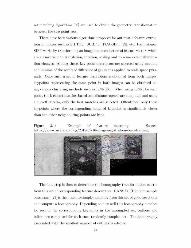
set matching algorithms [30] are used to obtain the geometric transformation

between the two point sets.

There have been various algorithms proposed for automatic feature extrac-

tion in images such as SIFT[46], SURF[6], PCA-SIFT [39], etc. For instance,

SIFT works by transforming an image into a collection of feature vectors which

are all invariant to translation, rotation, scaling and to some extent illumina-

tion changes. Among these, key point descriptors are selected using maxima

and minima of the result of difference of gaussians applied to scale space pyra-

mids. Once such a set of feature descriptors is obtained from both images,

keypoints representing the same point in both images can be obtained us-

ing various clustering methods such as KNN [65]. When using KNN, for each

point, the k-closest matches based on a distance metric are computed and using

a cut-off criteria, only the best matches are selected. Oftentimes, only those

keypoints where the corresponding matched keypoint is significantly closer

than the other neighbouring points are kept.

Figure 3.1: Example of feature matching. Source:https://www.sicara.ai/blog/2019-07-16-image-registration-deep-learning

The final step is then to determine the homography transformation matrix

from this set of corresponding feature descriptors. RANSAC (Random sample

consensus) [23] is then used to sample randomly from this set of good keypoints

and compute a homography. Depending on how well this homography matches

for rest of the corresponding keypoints in the unsampled set, outliers and

inliers are computed for each such randomly sampled set. The homography

associated with the smallest number of outliers is selected.

24

While these methods are quite fast, often the feature detector stage is the

bottleneck, so alternative faster feature detectors have been proposed such

as Oriented FAST and Rotated BRIEF (ORB) [60] which trade-off time for

performance.

• Pros: Very fast

• Cons: Can be quite inaccurate when:

1. The feature detector stage performs poorly

2. There aren’t enough detected keypoints

3. The keypoint matching stage performs poorly due to drastic changes

in illumination or large changes in viewing angles

3.2 Learning based approaches

Most learning based approaches are characterized by training a model to learn

the transformation between a registered pair of images where the ground truth

is available. In recent times, given the prevalence of CNNs as feature extrac-

tors, DeTone, Malisiewicz, and Rabinovich [18] proposed homography estima-

tion as a deep learning based supervised learning task. They posit that in

a homography matrix, estimating all parameters together is quite a difficult

optimization task, since it mixes the rotational and translational terms. They

propose to use an alternative four-point parametrization which works better.

They create a synthetic dataset using patches from the MS-COCO dataset [45]

which have been altered with random homography perturbations in a limited

range and use that as the training target.

Cheng, Zhang, and Zheng [15] hypothesize that a similarity metric for

multi-modal registration is usually too complex to be represented using inten-

sity based statistical metrics. So they propose learning the similarity metric

itself that is trained using a binary classifier to learn the correspondence of

two image patches.

• Pros: Very fast at inference

25

Figure 3.2: Structure of HomographyNet as proposed by DeTone, Malisiewicz,and Rabinovich [18]

• Cons:

1. Training time for an entire dataset can be quite long.

2. Needs annotated data.

3. Performance depends on size of training data available.

4. Not very robust to data not seen in the training set.

3.3 Optimization based approaches

This thesis primarily deals with ideas in this family of approaches. Opti-

mization based approaches work at the global level by using pixel to pixel

matching rather than extracting specialized features and computing descrip-

tors for them. The Lucas-Kanade algorithm [47] is one of the earliest such

approaches to doing this. It works by solving the optical flow equations for all

the pixels in the neighbourhood my minimizing the mean squares error.

This family of algorithms works by first deciding on a transformation/warping

model. This transformation could be deformable or non-deformable. In case

of deformable registration, the model is usually parametrized by a displace-

ment vector field and in case of non-deformable registration, the model is

paramtrized by a homography matrix. In this work we focus on non-deformable

registration transformations. The transformation model is often initialized

with a guess and a distance metric is used to compute the quality of the cur-

rent registration. Often a differentiable metric is preferred because gradient

descent based techniques for optimization work quite well to minimize such

a cost function as compared to search based optimization. A very intuitive

26

example of such a cost function is MSE (Mean Square Error) [4]. Often in

deformable registration, a weighted regularization term is added to the cost

function to enforce constraints, for eg. smoothness of displacement fields.

Since the transformation model focused on this work is homography based,

we look at it in more detail. The transformation parameters for the homog-

raphy matrix are often not optimized directly, but rather alternative methods

have been found to have better results. For instance, DeTone, Malisiewicz,

and Rabinovich [18] used a four-point parametrization approach. On the other

hand, Wachinger and Navab [80] parametrize 3D transformations using matrix

exponentials.

There have been attempts to improve the robustness of global optimiza-

tion based approaches by combining feature based methods [86] or proposing

different loss functions such as ECC (Enhanced Correlation Coefficient) [22]

or by representing images in the Fourier domain [48].

Nguyen et al. [55] proposed an unsupervised alternative, where they try to

use a four-point paramterization as well and use the L1 pixel-wise photometric

loss. There have been attempts to speed up optimization by using techniques

such as Gaussian pyramids (Section 2.2) or by improving optimization tech-

niques [53], which by themselves are an active area of research.

Given a univariate function f(w), the second order Taylor expansion of f

around an initial point w0 is:

f(w) ≈ f(w0) + (w − w0)f ′(w0) +1

2(w − w0)2f ′′(w0) (3.1)

A stationary point of this f(w) can be found by setting its first derivative to

0, i.e.:

f ′(w) ≈ f ′(w0) + (w − w0)f ′′(w0) = 0 (3.2)

Solving this we can get:

w1 = w0 −f ′(w0)

f ′′(w0)(3.3)

Performing this update in an iterative manner, we get the general equation:

wt+1 = wt −f ′(wt)

f ′′(wt)(3.4)

27

This is called Newton’s method of optimization or second-order gradient de-

scent. Depending on the number of terms used from Eqn. 3.1 we can also have

first-order gradient descent methods if we ignore the final second-order term.

This leads to more inaccurate but faster updates. The Levenberg–Marquardt

[44] algorithm is another such optimization technique which has been used for

solving non-linear least squares problems. In a multi-variate setting, comput-

ing the inverse of the second order term in Eqn. 3.4 becomes a very expensive

and slow process, hence, a third family of optimization techniques exist called

Quasi-Newton methods, which use an approximation of the inverse of the sec-

ond order term.

• Pros:

1. Needs no annotated training data.

2. Works for any pairwise registration task given a suitable cost func-

tion

• Cons:

1. Slower as compared to other approaches (at inference time)

28

Chapter 4

Proposed Multi-ResolutionImage Registration

In this section, we present two algorithms: DRMIME and ODECME. The

first, DRMIME, brings in the ideas of using MINE as a loss function and

using Matrix Exponential for parametrization. The second, ODECME, builds

on these ideas and further refines the algorithm by adding complex matrix

exponentials, ODEnet and a symmetric loss function.

4.1 Differentiable Mutual Information and Ma-

trix Exponential for Multi-Resolution Im-

age Registration

4.1.1 MINE for images

While MINE is a general purpose estimator for MI between any two n-dimensional

variables, we adapt it slightly as below (Algorithm 1) to use it for pairwise

image MI computation. Our objective as proposed in Eqn. 2.1 now becomes

(MI needs to be maximised for registration):

maxv1,v2,...

MINE(T,Warp(M,Mexp(∑i

viBi))). (4.1)

Algorithm 1 takes in two images X and Z along with a subset of pixel

locations I. It creates a random permutation Is of the indices I. Ij denotes

the jth entry in the index list I, while XIj denotes the Ithj pixel location on

29

Algorithm 1: MINE

MINE (X,Z, I)Input: Image X, Image Z, Sampled pixel locations IOutput: Estimated mutual information (DV lower bound)

Shuffle pixel locations: Is = RandomPermute(I) ;N = length(I) ;DV = 1

N

∑j fθ(XIj , ZIj)− log( 1

N

∑j exp(fθ(XIj , ZIsj ))) ;

Return DV ;

image X. Finally, the algorithm returns the DV lower bound [8] computed by

Monte Carlo approximation of (2.11).

Figure 4.1: Given a pair of images, MINE converges to the DV lower bound.

Using a multi-resolution approach, the cost function (Eqn. 4.1) becomes:

maxv1,...,v6

L∑l=1

MINE(Tl,Warp(Ml,Mexp(

6∑i=1

viBi))). (4.2)

However, note also that image structures are slightly shifted through multi-

resolution image pyramids. So, a transformation matrix suitable for a coarse

resolution may need a slight correction when used for a finer resolution. To

mitigate this issue, we exploit matrix exponential parameterization and intro-

duce an additional parameter vector v1 = [v11, ..., v

16] exclusively for the finest

resolution and modify optimization (4.2) as follows:

30

maxv1,··· ,v6v11 ,··· ,v16

θ

L∑l=2

MINE(Tl,Warp(Ml,Mexp(6∑i=1

viBi))) +MINE(T1,Warp(M1,Mexp(6∑i=1

(vi + v1i )Bi))),

(4.3)

where θ denotes the parameters of the neural network that MINE uses to

realize f .

4.1.2 DRMIME Algorithm

Fig. 4.2 shows a schematic for the optimization problem (4.3). Our proposed

algorithm DRMIME (Algorithm 2) implements DRMIME [54] that uses DV

lower bound (2.11) computed in turn by Algorithm 1, which employs a fully

connected neural network fθ MINEnet. MINEnet has two hidden layers with

100 neurons in each layer. We use ReLU non-linearity in both the hidden

layers. The Appendix contains details about other hyperparameters. The

code for DRMIME is available here.

Algorithm 2: DRMIME

Input: Fixed image T , moving image MOutput: Transformation matrix H1

Set learning rates α, β, γ and pyramid level L;Build multiresolution image pyramids TlLl=1 from T and MlLl=1

from M ;Use random initialization for MINEnet parameters θ ;Initialize v and v1 to the 0 vectors ;for each iteration do

MI = 0 ;

H = Mexp(∑6

i=1 viBi) ;

H1 = Mexp(∑6

i=1(vi + v1i )Bi) ;

I1 = Sample pixel locations on T1 ;MI+ = MINE(T1,Warp(M1, H1), I1) ;for l = [2, L] do

Il = Sample pixel locations on Tl ;MI+ = MINE(Tl,Warp(Ml, H), Il) ;

endUpdate MINEnet parameter: θ+ = α∇θMI ;Update matrix exponential parameters: v+ = β∇vMI andv1+ = γ∇v1MI;

end

Compute final transformation matrix: H1 = Mexp(∑6

i=1(vi + v1i )Bi) ;

31

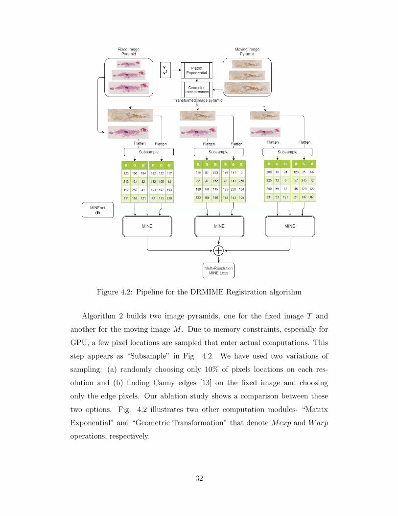
Figure 4.2: Pipeline for the DRMIME Registration algorithm

Algorithm 2 builds two image pyramids, one for the fixed image T and

another for the moving image M . Due to memory constraints, especially for

GPU, a few pixel locations are sampled that enter actual computations. This

step appears as “Subsample” in Fig. 4.2. We have used two variations of

sampling: (a) randomly choosing only 10% of pixels locations on each res-

olution and (b) finding Canny edges [13] on the fixed image and choosing

only the edge pixels. Our ablation study shows a comparison between these

two options. Fig. 4.2 illustrates two other computation modules- “Matrix

Exponential” and “Geometric Transformation” that denote Mexp and Warp

operations, respectively.

32

4.2 Ordinary Differential Equation and Com-

plex Matrix Exponential for Multi-resolution

Image Registration

With DRMIME, we notice that we use the same parameters for all multi-

resolution levels except the last. The intuition still remains that all levels

need some additional changes from the previous level, which implies that all

levels ideally have their own coefficients and the change from one level to the

next is related in some manner. We can model the dynamics of these changes

to improve performance of the registration algorithm. Furthermore, due to the

surjectivity of the real valued matrix exponential many geometric transforma-

tion matrices in the vector space cannot be reached and this could potentially

hurt performance. We remedy this by using complex matrix exponential.

4.2.1 ODE for Multi-resolution Image Registration

Image structures are slightly shifted through multi-resolution Gaussian image

pyramids [82]. So, a transformation matrix suitable for a coarse resolution

may need a slight correction when used for a finer resolution. To mitigate

this issue, we model matrix exponential parameters as a continuous function

v(s) of resolution s. The change in v(s) over resolution s can be modeled by a

neural network gφ with parameters φ:

dv(s)

ds= gφ(s, v(s)). (4.4)

The added benefit of using a neural network as the function g is that neural

networks are differentiable and hence, using the autograd feature of modern

packages (e.g., PyTorch, Tensorflow) we can easily compute derivatives for

updating the parameters of the neural network.

Using Euler method [11] the ordinary differential equation (ODE) (4.4) can

be solved for all resolution levels 1, 2, ..., L:

vL = u

for l = L− 1, L− 2, · · · , 1

vl = vl+1 + (sl − sl+1)gφ(sl+1, vl+1),

(4.5)

33

where vl = [vl,1, vl,2, ...] are the matrix exponential coefficients for resolution

level l and sl = d−l+1, l = 1, 2, .., L denote the discrete resolutions in powers

of the downscale factor d. u = [u1, u2, ...] is the initial value vector in the ODE

and it is an optimizable parameter of the model along with the neural network

parameters φ. We have also used 4-point Runge-Kutta method (RK4) [11] for

the above recursion:

vL = u

for l = L− 1, L− 2, · · · , 1

h = sl − sl+1,

k1 = hgφ(sl+1, vl+1),

k2 = hgφ(sl+1 + 13h, vl+1 + 1

3k1),

k3 = hgφ(sl+1 + 23h, vl+1 − 1

3k1 + k2),

k4 = hgφ(sl, vl+1 + k1 − k2 + k3),

vl = vl+1 + 18(k1 + 3k2 + 3k3 + k4).

(4.6)

Generating matrix exponential coefficients vl, l = 1, 2, .., L by the ODE so-

lution (4.5) or (4.6), the optimization for image registration (4.9) using mutual

information now becomes:

maxu1,u2,···φ,θ

L∑l=1

MINE(Tl,Warp(Ml,Mexp(∑i

vl,iBi)))+

MINE(Ml,Warp(Tl,Mexp(−∑i

vl,iBi))).(4.7)

4.2.2 Symmetric loss function

Usually in image registration tasks, only the moving image is transformed and

then a cost function is used to compute the distance metric between the fixed

image and the transformed moving image. Given the entire multi-resolution

pyramid the cost function (Eqn. 4.1) is then:

minv1,v2,...

L∑l=1

D(Tl,Warp(Ml,Mexp(∑i

viBi))) (4.8)

Since we use matrix exponential coefficients to parametrize our transform, it

is very simple to compute the inverse transform and apply it to the moving

image. Computing the inverse is as straightforward as:

34

H−1 = Mexp(−∑

i viBi)

This way we add an additional term to our cost function, which is the cost of

registering the fixed image to the moving image as well.

minv1,v2,...

L∑l=1

D(Tl,Warp(Ml,Mexp(∑i

viBi)))+

D(Ml,Warp(Tl,Mexp(−∑i

viBi))),(4.9)

This alters our objective of registering one moving image to a fixed image

and changes it to an objective where we register the images to each other

mutually. This symmetric cost function is likely to help make the registration

much more robust since the geometric transform and its inverse both need to

be correct simultaneously, but also at the same time they remain parametrized

by common parameters which are optimized at the same time.

4.2.3 Complex Matrix Exponential

It is well known that exponential of real valued matrix is not globally surjective,

i.e., not all transformation matrices (affine or homography) can be obtained by

the exponential of real-valued matrices [24]. One way to overcome this issue

is to compose matrix exponential a few times to compute the transformation

matrix.

In this work, we propose to use complex matrix exponential an alterna-

tive to the scheme using composition, because complex matrix exponential is

globally surjective [24]. Thus, a complex matrix, Br +√−1Bi =

∑i viBi, pro-

duced by complex parameters, vi = vri +√−1vii, can use matrix exponential

series (2.15) to create a complex transformation matrix,

Hr +√−1H i = Mexp(Br +

√−1Bi). (4.10)

Next, we choose to transform a point (x, y) to another point (x′, y′) using the

following:

[xr, yr, zr]T = Hr[x, y, 1]T , [xi, yi, zi]T = H i[x, y, 1]T ,

x′ =xrzr + xizi

(zr)2 + (zi)2, y′ =

yrzr + yizi

(zr)2 + (zi)2.

(4.11)

35

Figure 4.3: Randomly generated grids by complex matrix exponential (4.10)and complex transformation (4.11). Elements of Br were generated by a zeromean Gaussian with 0.1 standard deviation (SD) for all four panels. Elementsof Bi were generated by a zero mean Gaussian with SD as follows: 0 fortop-left, 0.1 for top-right, 0.2 for bottom-left and 0.3 for bottom-right panel.

Note that under our chosen transformation (4.11) the straight lines are

not guaranteed to remain straight. However, if H i = 0, transformation (4.11)

degenerates to a linear transformation using homogeneous coordinates. Fig.

4.3 shows four randomly generated grids using (4.10) and (4.11). When imag-

inary coefficients are zeros (top-left panel, where Bi = 0 and consequently

H i = 0), the transformation acts as a homography, whereas the degree of the

non-linearity in the transformation increases as the magnitude of Bi increases.

Unlike, a 2D Mobius transformation [40], the proposed complex transformation

does not guarantee self-intersection. However, note that 2D Mobius transfor-

mation is more restrictive, as for example, it cannot generate a perspective

transformation.

4.2.4 ODECME Algorithm

Combining the aforementioned elements, ordinary differential equation (ODE)

(Section 4.2.1) and complex matrix exponential (CME) (Section 4.2.3), our

proposed Algorithm 3 (ODECME) first builds two image pyramids, one for

the fixed and another for the moving image. It then computes Euler recursion

for ODE-based computation of CME coefficients. Alternatively, we have also

36

used RK4 recursion (4.6) in our experiments. Note also that “Mexp” may

refer to real or complex matrix exponential, depending on whether u and vl

are complex or real. Also, “MINE” can be replaced by any differentiable loss

for image registration. “MINEnet” in Algorithm 3 denotes fθ, (refer to (2))

which is a fully connected neural network [54]. “ODEnet” refers to the fully

connected neural network gφ appearing in (4.5) and (4.6). Taking advantage

of matrix exponential, we use symmetric loss, which uses both the forward

and the inverse transformation matrices. For any gradient computation, such

as ∇θMI or ∇φMI, we use autograd (bult-in optimizers) of PyTorch [56].

Algorithm 3 finally outputs original resolution transformation matrix and its

inverse.

Figure 4.4: Pipeline for the ODECME Registration algorithm (using multi-resolution pyramid of 3 levels)

37

Algorithm 3: ODECME

Build multiresolution image pyramids Tl,MlLl=1 ;Set learning rates α, β and γ;Use random initialization for MINEnet parameters θ ODEnetparameters φ ;

Initialize u to the 0 vector ;for each iteration do

vL = u ;HL = Mexp(

∑i vL,iBi) ;

H−1L = Mexp(−

∑i vL,iBi) ;

for l = [L− 1, .., 1] dovl = vl+1 + (sl − sl+1)fφ(sl+1, vl+1) ;Hl = Mexp(

∑i vl,iBi) ;

H−1l = Mexp(−

∑i vl,iBi) ;

endMI = 0 ;for l = [1, L] do

MI+ = MINE(Tl,Warp(Ml, Hl)) ;MI+ = MINE(Ml,Warp(Tl, H

−1l )) ;

endUpdate MINEnet parameter: θ+ = α∇θMI ;Update ODEnet parameter: φ+ = β∇φMI ;Update matrix exponential parameter: u+ = γ∇uMI ;

endCompute final transformation matrices:vL = u ;for l = [L− 1, .., 1] do

vl = vl+1 + (sl − sl+1)fφ(sl+1, vl+1) ;endH1 = Mexp(

∑i v1,iBi) ;

H−11 = Mexp(−

∑i v1,iBi);

38

Chapter 5

Experiments

5.1 Datasets

The datasets chosen for our experiments correspond to testing two important

hypotheses. First, performing image registration with our algorithm on images

within the same modality fares comparably (or better) to other standard algo-

rithms. For this, we use the FIRE (Fundus Image Registration) dataset [31].

Second, since our algorithm is based on MI, it can handle multi-modal regis-

tration successfully as well. For this we use data from the ANHIR (Automatic

Non-rigid Histological Image Registration) 2019 challenge[10].

Furthermore, since Mutual Information can be used even for volumetric

data, we applied our algorithm to the IXI (Information eXtraction from Im-

ages) dataset 1 for testing mono-modal registration performance and the ADNI

(Alzheimer’s Disease Neuroimaging Initiative) dataset [85] for multi-modal

registration.

5.1.1 FIRE

The FIRE dataset consists of 134 retinal fundus image pairs. These pairs are

classified into three categories depending on what purpose they were collected

for: S (Super resolution, 71 pairs), P (Mosaicing, 49 pairs) and A (Longitu-

dinal Study, 14 pairs). Of these, Category P pairs have < 75% overlap which

provides a near impossible challenge for gradient based algorithms, not just

ours, but also for the competing algorithms. The registration optimization

1IXI dataset: https://brain-development.org/ixi-dataset/

39

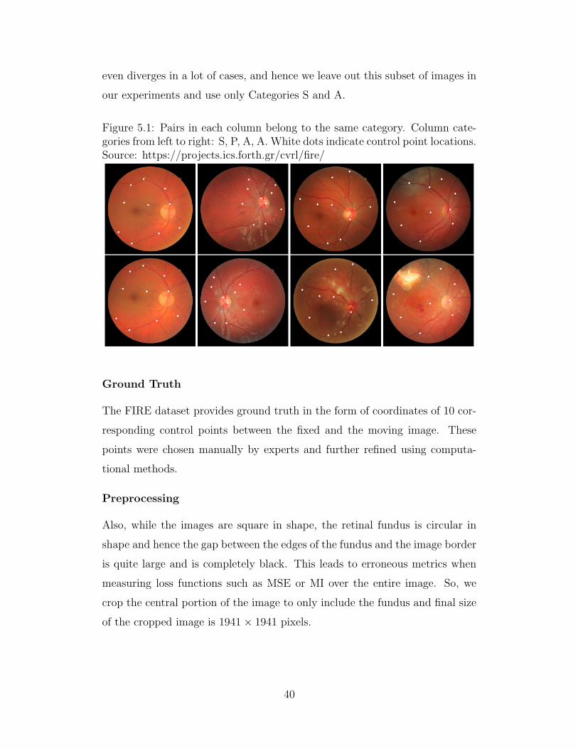
even diverges in a lot of cases, and hence we leave out this subset of images in

our experiments and use only Categories S and A.

Figure 5.1: Pairs in each column belong to the same category. Column cate-gories from left to right: S, P, A, A. White dots indicate control point locations.Source: https://projects.ics.forth.gr/cvrl/fire/

Ground Truth

The FIRE dataset provides ground truth in the form of coordinates of 10 cor-

responding control points between the fixed and the moving image. These

points were chosen manually by experts and further refined using computa-

tional methods.

Preprocessing

Also, while the images are square in shape, the retinal fundus is circular in

shape and hence the gap between the edges of the fundus and the image border

is quite large and is completely black. This leads to erroneous metrics when

measuring loss functions such as MSE or MI over the entire image. So, we

crop the central portion of the image to only include the fundus and final size

of the cropped image is 1941× 1941 pixels.

40

Evaluation

For evaluating registration accuracy, we compute the Euclidean distance be-

tween these corresponding points after registration and average them. Also the

image coordinates are scaled to be between 0 and 1 so that images of different

sizes can be compared using the same benchmark. We call this measure the

Normalized Average Euclidean Distance (NAED). Most competing methods

do not support a homography based registration model, so an affine model

was used to be consistent all across.

5.1.2 ANHIR

The ANHIR (Automatic Non-rigid Histological Image Registration) dataset

provides high-resolution histopathological tissue images stained with different

dyes. This provides a multi-modal challenge.

Figure 5.2: Different types of samples in ANHIR. Source: https://anhir.grand-challenge.org/

Ground Truth

The ground truth provided is similar to the FIRE dataset, except for the fact

that more than 10 corresponding coordinates might be provided as the ground

41

truth in certain pairs. Also, we use only the training set provided in the

database, since only those pairs (230) have the ground truth available.

Preprocessing

The ANHIR dataset has some incredibly large resolution images (upto 100k×

200k pixels). Some of the competing registration frameworks were unable to

process such large images and so, we downscaled every image by a factor of 5 to

make them available to every framework. Furthermore, each staining can have

a different resolution as well, so the fixed and moving image pairs need not be

the same size. So, to remedy this, we rescale the image with a smaller aspect

ratio to match the width of the paired image. Post that the height is padded

to match the other image as well. This preprocessing is consistent across all

algorithms and allows us to maintain the aspect ratios of the individual images

and have both images in a pair at the same resolution without any distortions.

Evaluation

We use NAED as the evaluation metric here as well and use an affine model

for transformation.

5.1.3 IXI

The IXI dataset has about 600 MR images from healthy patients. It includes

T1, T2, PD-weighted images, MRA images, and Diffusion-weighted images.

Preprocessing

We choose 51 T1 volumes (at random) which have the same size and designate

one as the Atlas (reference volume) and register the other 50 volumes against

it. All the voxel intensity values were normalised.

Evaluation

Unfortunately, the IXI dataset does not come with any form of ground truth, so

we resort to standard measures [28] for registration accuracy such as SSIM[64],

PSNR[63] and SSD (Sum of Squared Differences). The SSIM, PSNR, SSD

42

scores are computed after every registration with the Atlas and averaged and

then reported for each algorithm. The transformation model used has 7 degrees

of freedom, composed of isotropic scaling with three axes of rigid transforma-

tion and three axes for rotation.

5.1.4 ADNI

The ADNI dataset provides 1.5T and 3T MRI scans of patients scanned over

different periods of time.

Preprocessing

We chose one volume as the atlas (reference volume) from the ADNI1:Screening

1.5T collection and another 50 volumes from the ADNI1:Baseline 3T collec-

tion. All voxel intensity values were normalized, and resized to match the

reference volume (160× 192× 192) before feeding into any of the algorithms.

Evaluation

Similar to the IXI dataset, no groundtruth is available here too, so we report

the averaged SSIM and PSNR metrics for the dataset after registration. The

transformation model used has 7 degrees of freedom, composed of isotropic

scaling with three axes of rigid transformation and three axes for rotation.

5.2 Competing algorithms

We evaluate our method against the following off-the-shelf registration algo-

rithms from popular registration frameworks. The competing algorithms were

whether they use MI or can be used for multi-modal registration:

1. Mattes Mutual Information (MMI) [50, 51, 36]: As mentioned in

equation (2.6), we need to compute the joint and marginal probabilities

of the fixed and moving images. To reduce the effects of quantization

from interpolation and discretization due to binning, this version of MI

computation uses Parzen windowing to form continuous estimates of the

underlying image histogram.

43

2. Joint Histogram Mutual Information (JHMI) [76, 35]: This method

computes Mutual Information using Parzen windows as well, but it uses

separable Parzen windows. By selection of a Parzen window that satis-

fies the partition of unity, it provides a tractable closed-form expression

of the gradient of the MI computation with respect to transformation

parameters.

3. Normalized Cross Correlation (NCC)[38]: As the names says, the

correlation between the moving and the fixed image pixel intensities is

computed. The correlation is normalized by the autocorrelations of both

the fixed and moving images.

4. Mean Square Error (MSE)[37]: This is the mean squared difference

of the pixelwise intensity between the fixed and moving image.

5. AirLab Mutual Information (AMI)[61]: AirLab is a PyTorch based

image registration framework. It performs histogram based mutual infor-

mation computation[79, 49]. Since it is a deep learning based solution, it

provides support for using batches as well as state-of-the-art optimizers

and GPU support.

6. Normalized Mutual Information (NMI)[68, 41]: The initial PDF

(probability density function) construction is done using Parzen his-

tograms, and then MI is obtained by double summing over the discrete

PDF values. In this metric, the final MI is normalized to a range between

0 and 1.

Also as a note, most libraries limit 2D image registration to affine trans-

forms in terms of degrees of freedom. While it is possible to use perspective

transforms with our algorithm just by changing the base vector (v), in order

to have a fair comparison, we limit our algorithm to affine transforms as well.

In case of 3D volume registration, since the highest degree of freedom for

geometric transforms supported for 3D volumes is the similarity transform,

that is what we use for comparison. It consists of a rotation, translation and

44

isotropic scaling to the space. The implementations of the above algorithms

were used from these packages:

• SITK[67]: MMI, JHMI, NCC, MSE

• AirLab[1]: AMI

• SimpleElastix[66]: NMI

In terms of sampling, we noticed using Canny edge-detection based sampling

helps registration results slightly. In the following results, the DRMIME al-

gorithm uses Canny sampling. We look at its effects in the ablation study

(Section 5.4.3). Since other frameworks don’t have access to such a pre-

processing step in their pipeline, to ensure a fair comparision between them

and ODECME, we use random sampling, the hyperparameters for which are

in the Appendix (Section A.2).

5.3 Results

This section lists the results for all algorithms on the aforementioned datasets.

For all evaluations, we also conduct a paired t-test with DRMIME (with real

matrix exponential) to investigate if the results are statistically significant (p-

value < 0.05). These p-values show that the changes brought in by DRMIME

were statistically significant (or not) compared to other algorithms available in

registration toolboxes; and also if elements added by ODECME led to results

statistically significantly different to DRMIME. Please note, unless explicitly

mentioned, DRMIME refers to the vanilla version of DRMIME which uses just

real matrix exponential.

Fig. 5.3 shows registration results for a random FIRE sample. Table

5.1 shows the NAED for all algorithms on the FIRE dataset. Here, DR-

MIME/ODECME performs almost an order of magnitude better than the

competing algorithms and the results are statistically significant.

45

Figure 5.3: The images on the left show a pair to be registered from theFIRE dataset. The images on the right represent the difference between thetransformed moving image and the fixed image after registration by differentalgorithms. Source: Nan et al. [54]

Table 5.1: NAED for FIRE dataset along with paired t-test significance valuesAlgorithm NAED (Mean ± STD) p-value

ODE (RK4-Complex) 0.00381 ± 0.010 0.0032ODE (RK4-Real) 0.00385 ± 0.014 0.0032

DRMIME (Complex) 0.00482 ± 0.031 0.1021DRMIME (Real) 0.00482 ± 0.014 -

ODE (Euler-Complex) 0.0049 ± 0.016 0.0822ODE (Euler-Real) 0.0049 ± 0.016 0.1053

NCC 0.0194 ± 0.033 1.3e-04MMI 0.0198 ± 0.034 5.4e-05NMI 0.0228 ± 0.032 1.7e-08JHMI 0.0311 ± 0.046 4.5e-07AMI 0.0441 ± 0.028 1.4e-27MSE 0.0641 ± 0.094 3.5e-03

Fig. 5.4 presents a closer look at the same metrics from Table 5.1. We note

46

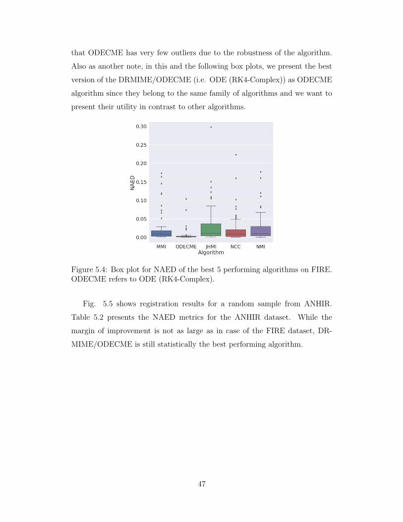
that ODECME has very few outliers due to the robustness of the algorithm.

Also as another note, in this and the following box plots, we present the best

version of the DRMIME/ODECME (i.e. ODE (RK4-Complex)) as ODECME

algorithm since they belong to the same family of algorithms and we want to

present their utility in contrast to other algorithms.

Figure 5.4: Box plot for NAED of the best 5 performing algorithms on FIRE.ODECME refers to ODE (RK4-Complex).

Fig. 5.5 shows registration results for a random sample from ANHIR.

Table 5.2 presents the NAED metrics for the ANHIR dataset. While the

margin of improvement is not as large as in case of the FIRE dataset, DR-

MIME/ODECME is still statistically the best performing algorithm.

47

Figure 5.5: The images on the left show a pair to be registered from theANHIR dataset. The images on the right represent the difference between thetransformed moving image and the fixed image after registration by differentalgorithms.

Table 5.2: NAED for ANHIR dataset along with paired t-test significancevalues

Algorithm NAED (Mean ± STD) p-value

ODE (RK4-Complex) 0.0345 ± 0.050 0.0441ODE (RK4-Real) 0.0348 ± 0.044 0.0642

ODE (Euler-Complex) 0.0361 ± 0.084 1.0e-03ODE (Euler-Real) 0.0391 ± 0.035 1.5e-03DRMIME (Real) 0.0384 ± 0.087 -

DRMIME (Complex) 0.0373 ± 0.021 0.0619NCC 0.0461 ± 0.084 7.0e-04MMI 0.0490 ± 0.082 6.2e-05MSE 0.0641 ± 0.094 5.5e-14NMI 0.0765 ± 0.090 3.0e-31AMI 0.0769 ± 0.090 3.7e-30JHMI 0.0827 ± 0.100 8.3e-21

The box-plots in Fig. 5.6 also emphasise the same conclusion as we saw

before, i.e. ODECME outperforms the other competing algorithms.

48

Figure 5.6: Box plot for top 5 performing algorithms on ANHIR. ODECMErefers to ODE (RK4-Complex).

For results on the IXI dataset, we compute the SSIM, PSNR and MSE

score after registration and present them in Fig. 5.7, 5.8, 5.9 respectively.

Figure 5.7: Box plot for SSIM values (higher is better) for each algorithm onthe IXI datset after registration. ODECME refers to ODE (RK4-Complex).

49

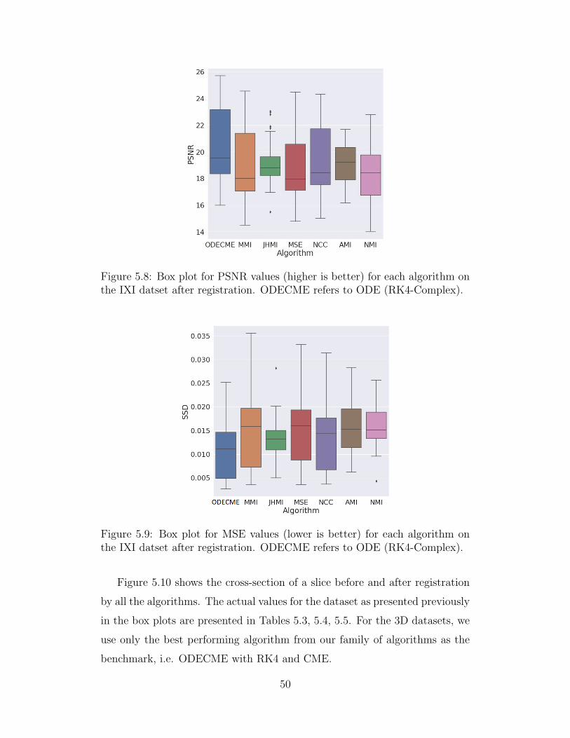
Figure 5.8: Box plot for PSNR values (higher is better) for each algorithm onthe IXI datset after registration. ODECME refers to ODE (RK4-Complex).

Figure 5.9: Box plot for MSE values (lower is better) for each algorithm onthe IXI datset after registration. ODECME refers to ODE (RK4-Complex).

Figure 5.10 shows the cross-section of a slice before and after registration

by all the algorithms. The actual values for the dataset as presented previously

in the box plots are presented in Tables 5.3, 5.4, 5.5. For the 3D datasets, we

use only the best performing algorithm from our family of algorithms as the

benchmark, i.e. ODECME with RK4 and CME.

50

Figure 5.10: The images on the left show the middle slice of a pair of volumesto be registered from the IXI dataset. The images on the right represent thedifference between the middle slices of the transformed moving volume andthe fixed volume after registration by different algorithms.

Table 5.3: SSIM for IXI dataset along with paired t-test significance valuesAlgorithm SSIM (Mean ± STD) p-value

ODE (RK4-Complex) 0.698897 ± 0.043251 -NMI 0.676213 ± 0.039430 7.22e-08AMI 0.673859 ± 0.041827 1.03e-20NCC 0.665657 ± 0.043032 6.95e-21MSE 0.652308 ± 0.040589 9.04e-19JHMI 0.644142 ± 0.036340 6.20e-22MMI 0.580596 ± 0.048000 6.04e-26

51

Table 5.4: PSNR for IXI dataset along with paired t-test significance valuesAlgorithm PSNR (Mean ± STD) p-value

ODE (RK4-Complex) 20.652895 ± 2.700216 -NMI 19.451672 ± 2.534976 1.85e-05MMI 19.266031 ± 1.623640 6.97e-28NCC 19.183119 ± 2.655105 6.78e-26AMI 18.999632 ± 1.437429 1.49e-20MSE 18.938889 ± 2.410362 7.93e-24JHMI 18.417178 ± 2.100850 7.56e-08

Table 5.5: MSE for IXI dataset along with paired t-test significance valuesAlgorithm MSE (Mean ± STD) -

ODE (RK4-Complex) 0.010224 ± 0.005447 -JHMI 0.012630 ± 0.004336 8.22e-08NCC 0.013196 ± 0.006556 3.41e-18MMI 0.014214 ± 0.007280 2.34e-17MSE 0.014594 ± 0.006722 3.86e-22AMI 0.015413 ± 0.005074 3.71e-05NMI 0.015845 ± 0.004178 7.91e-07

For the ADNI dataset, we look at the SSIM and PSNR values post-registration

in Figures 5.11,5.12 and Tables 5.7, 5.6.

Figure 5.11: Box plot for SSIM values (higher is better) for each algorithmon the ADNI dataset after registration. ODECME refers to ODE (RK4-Complex).

52

Figure 5.12: Box plot for PSNR values (higher is better) for each algorithmon the ADNI dataset after registration. ODECME refers to ODE (RK4-Complex).

Table 5.6: SSIM for ADNI dataset along with paired t-test significance valuesAlgorithm SSIM (Mean ± STD) p-value

ODE (RK4-Complex) 0.716824 ± 0.020805 -MSE 0.708778 ± 0.024048 0.000267AMI 0.691885 ± 0.040358 0.0006864MMI 0.687028 ± 0.038504 4.33e-09NCC 0.676213 ± 0.039430 3.82e-09NMI 0.665249 ± 0.031078 3.54e-14JHMI 0.600950 ± 0.019171 6.20e-22

Table 5.7: PSNR for ADNI dataset along with paired t-test significance valuesAlgorithm PSNR (Mean ± STD) p-value

ODE (RK4-Complex) 20.133869 ± 0.550024 -MSE 19.801862 ± 0.533838 5.22e-10NCC 19.451672 ± 2.534976 0.00657MMI 19.409420 ± 0.612595 3.73e-17AMI 19.092219 ± 0.790758 2.79e-10NMI 18.228307 ± 1.795898 3.36e-09JHMI 17.762530 ± 0.433996 9.46e-28

53

5.4 Ablation study

In this section we perform several ablation studies to have an understanding

of the roles of all the components used in DRMIME and ODECME, such as

multi-resolution pyramids, matrix exponential, complex matrix exponential,

ODE and smart feature selection via Canny edge detection. We compare

the performance of DRMIME/ODECME to versions of it without using the

aforementioned components. For all experiments, we again perform a paired

t-test between the with and without versions and report the p-value to check

for statistical significance.

5.4.1 Effect of multi-resolution

All hyperparameters are kept the same in the with and without experiments,

the only difference being in the with multi-resolution experiment we use 6

levels of the Gaussian pyramids in the DRMIME algorithm, whereas in the

without experiment we have a single level which is the native resolution of the

image. Table 5.8 lists the results for these experiments.

Table 5.8: NAED for DRMIME with and without using multi-resolution pyra-mids. P-value is from paired t-test between both cases.

Dataset DRMIME Without MultiRes p-value

FIRE 0.0048 ± 0.014 0.0043 ± 0.014 0.365ANHIR 0.0384 ± 0.087 0.1089 ± 0.150 1.78e-15

While the idea of multi-resolution was introduced in image registration

to facilitate optimization, we note that many of the off-the-shelf algorithms

have the same learning rate for all levels. As we are working with only an

approximation of the distribution of the original data at different levels of the

pyramid, there is a small chance that optimization at a particular sublevel

could diverge. This leads to poor registration results occasionally. In our

implementation of DRMIME, we produce batches which include data from

all levels of the pyramid, making the optimization process much more robust,

54

faster and less prone to divergence. Fig. 5.4 provides evidence to this since

very few results fall outside the interquartile range (as comapared to other

algorithms).

5.4.2 Effect of matrix exponentiation

All hyperparameters are again kept the same in the with and without experi-

ments; the only difference being, that rather than using a matrix exponential

based parametrization, we now have 6 parameters indicating the degrees of

freedom of an affine transform in a transformation matrix, i.e.θ1 θ2 θ3

θ4 θ5 θ6

0 0 1

.

Table 5.9: NAED for MINE with and without using manifolds. P-value isfrom paired t-test between both cases.

Dataset DRMIME Without Manifolds p-value

FIRE 0.0048 ± 0.014 0.0045 ± 0.015 0.4933ANHIR 0.0384 ± 0.087 0.0580 ± 0.134 0.0012

Table 5.9 presents the results for these experiments. While the ablation

study on the FIRE dataset results in similar results, the p-values from the

paired t-test tells us that the results are not very significant to be able to

conclude anything. The ANHIR datset on the other hand sees a statistically

significant improvement with use of matrix exponentiation.

5.4.3 Effect of Sampling strategy

It could be argued that our smart feature extraction via Canny edge detection

helps DRMIME perform better than other algorithms, since other algorithms

do not have such custom feature detectors embedded in their pipeline. In order

to reduce this potential confounding variable, we also assessed the performance

of DRMIME with random sampling as well to make a fair comparison.

55

Table 5.10: NAED for DRMIME with Canny edge detection and RandomSampling (10%). P-value is from paired t-test between both cases.

Dataset With Canny Random Sampling(10%) p-value

FIRE 0.0048 ± 0.014 0.0097 ± 0.026 0.0296ANHIR 0.0384 ± 0.087 0.0588 ± 0.167 0.0333

Table 5.10 presents these results. As can be seen, there is a small drop in

performance, but DRMIME still performs better than all the algorithms from

other registration toolboxes with FIRE (Table 5.1) and better than most other

algorithms with ANHIR (Table 5.2). It is important to note, that DRMIME

results are using only 10% sampling, whereas the other algorithms use 50%

sampling (see Appendix) due to limited memory available on the GPU.

5.4.4 Effect of CME

In order to understand how using complex matrix exponentials affect our al-

gorithm empirically, we performed an ablation study. While the NAED per-

formance results between DRMIME(Real) and DRMIME(Complex) in Tables

5.2 and 5.4 were not statistically significant to be able to conclusively con-

clude better accuracy, it does indeed speed up convergence. For instance, with

real matrix exponential, for the FIRE dataset, it takes about 500 epochs to

converge, while with ANHIR it takes about 1500 epochs. In case of complex

matrix exponential, it only takes about 300 epochs in case of FIRE, and about

1300 epochs for ANHIR. Figure 5.16 shows the NAED convergence graphs for

10 randomly selected pairs from FIRE.

56

Figure 5.16: NAED averaged for 10 randomly selected pairs from FIRE, plot-ted over 500 epochs. The error bars represent the standard deviation.

5.4.5 Effect of ODE

To demonstrate that the ODECME Algorithm (Algorithm 3) can indeed fine-

tune transformation matrices over the resolution levels, Fig. 5.17 shows vari-

ations of 6 coefficients generated by the ODE over different resolution levels.

These coefficients were obtained by registering a pair of images from the FIRE

dataset. It shows that the proposed ODE can adapt to the needs of the edges

and structures as they are shifted in the Gaussian pyramids.

57

Figure 5.17: Plot showing how individual coefficients generated by ODEnetvary with successive resolution levels. Level 0 is the original image and 4denotes the coarsest resolution.

Table 5.11 shows that for every matrix exponential coefficient (real and

imaginary) varies over a range. The average was computed over the range of

a coefficient across all image pairs after registration.

Table 5.11: The average range and standard deviation of real and imaginarycoefficients after registering the FIRE dataset

Coefficient (Real) Mean Range ± SD (Imag.) Mean Range ± SD

v0 5.772e-03 ± 5.516e-03 5.771e-03 ± 5.515e-03v1 9.540e-03 ± 8.420e-03 9.537e-03 ± 8.414e-03v2 5.745e-03 ± 5.479e-03 5.745e-03 ± 5.476e-03v3 8.796e-03 ± 9.861e-03 8.796e-03 ± 9.854e-03v4 5.657e-03 ± 5.090e-03 5.664e-03 ± 5.088e-03v5 6.951e-03 ± 4.716e-03 7.068e-03 ± 4.796e-03

5.5 Efficiency

For efficiency we look at two perspectives: time efficiency and accuracy. On

a set of 10 randomly selected images (the set remains the same across all

algorithms) from the FIRE dataset, we run a set of experiments for all the

58

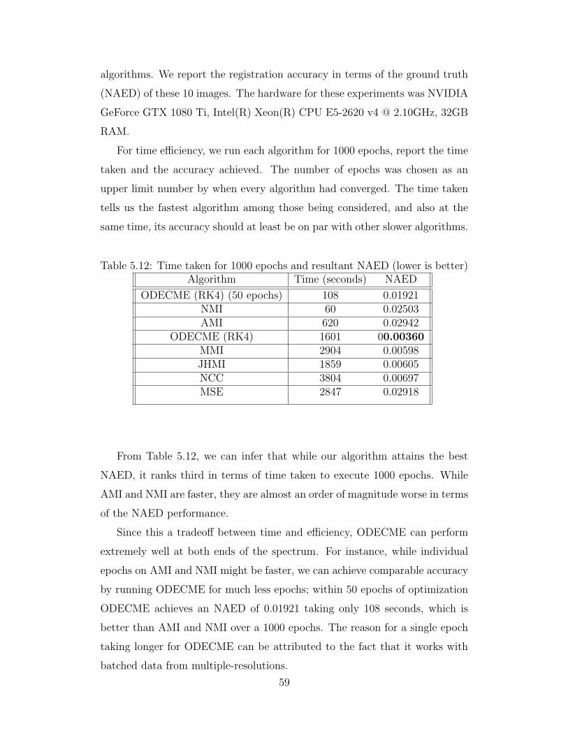
algorithms. We report the registration accuracy in terms of the ground truth

(NAED) of these 10 images. The hardware for these experiments was NVIDIA

GeForce GTX 1080 Ti, Intel(R) Xeon(R) CPU E5-2620 v4 @ 2.10GHz, 32GB

RAM.

For time efficiency, we run each algorithm for 1000 epochs, report the time

taken and the accuracy achieved. The number of epochs was chosen as an

upper limit number by when every algorithm had converged. The time taken

tells us the fastest algorithm among those being considered, and also at the

same time, its accuracy should at least be on par with other slower algorithms.

Table 5.12: Time taken for 1000 epochs and resultant NAED (lower is better)Algorithm Time (seconds) NAED

ODECME (RK4) (50 epochs) 108 0.01921NMI 60 0.02503AMI 620 0.02942

ODECME (RK4) 1601 00.00360MMI 2904 0.00598JHMI 1859 0.00605NCC 3804 0.00697MSE 2847 0.02918

From Table 5.12, we can infer that while our algorithm attains the best

NAED, it ranks third in terms of time taken to execute 1000 epochs. While

AMI and NMI are faster, they are almost an order of magnitude worse in terms

of the NAED performance.

Since this a tradeoff between time and efficiency, ODECME can perform

extremely well at both ends of the spectrum. For instance, while individual

epochs on AMI and NMI might be faster, we can achieve comparable accuracy

by running ODECME for much less epochs; within 50 epochs of optimization

ODECME achieves an NAED of 0.01921 taking only 108 seconds, which is

better than AMI and NMI over a 1000 epochs. The reason for a single epoch

taking longer for ODECME can be attributed to the fact that it works with

batched data from multiple-resolutions.

59

Also as a note, only ODECME/DRMIME and AMI are GPU compatible,

while the remaining were run on CPU.

60

Figure 5.13: Randomly selected slices from the difference volume before regis-tration between the reference and a randomly moving volume from the ADNIdataset. Each row represents slices from a different axis.

Figure 5.14: Same slices from the difference volume after registration usingODECME.

Figure 5.15: Same slices from the difference volume after registration usingMSE. 61

Chapter 6

Conclusion

Optimization-based image registration using homography as a transformation

is classical. However, recent toolboxes with autograd capability and strong

GPU acceleration has created opportunity to improve this classical registra-

tion algorithms. In this work, we show that using complex matrix exponential

convergence can be accelerated for such algorithms. Also using ordinary dif-

ferential equation, we can further refine the accuracy of such algorithms for

multi-resolution image registration problems that is able to employ any differ-

entiable objective function. Our algorithm yields state-of-the-art accuracy for

benchmark 2D and 3D datasets.

62

References

[1] airlab. airlab. url: https://github.com/airlab-unibas/airlab(visited on 07/31/2020).

[2] Haikel Salem Alhichri and Mohamed Kamel. “Multi-resolution imageregistration using multi-class Hausdorff fraction.”In: Pattern recognition letters 23.1-3 (2002), pp. 279–286.

[3] Yali Amit. “Graphical shape templates for automatic anatomydetection with applications to MRI brain scans.”In: IEEE Transactions on Medical Imaging 16.1 (1997), pp. 28–40.

[4] Simon Baker and Iain Matthews.“Lucas-kanade 20 years on: A unifying framework.”In: International journal of computer vision 56.3 (2004), pp. 221–255.

[5] Arindam Banerjee. “On bayesian bounds.” In: Proceedings of the 23rdinternational conference on Machine learning. 2006, pp. 81–88.

[6] Herbert Bay, Tinne Tuytelaars, and Luc Van Gool.“Surf: Speeded up robust features.”In: European conference on computer vision. Springer. 2006,pp. 404–417.

[7] Erik Johannes Bekkers et al.“Template matching via densities on the roto-translation group.”In: IEEE transactions on pattern analysis and machine intelligence40.2 (2017), pp. 452–466.

[8] Mohamed Ishmael Belghazi et al.“Mine: mutual information neural estimation.”In: arXiv preprint arXiv:1801.04062 (2018).

[9] FL Bookstein and WDK Green.“A thin-plate spline and the decomposition of deformations.”In: Mathematical Methods in Medical Imaging 2 (1993), pp. 14–28.

[10] Jirı Borovec et al. “ANHIR: automatic non-rigid histological imageregistration challenge.”In: IEEE Transactions on Medical Imaging (2020).

63

[11] J.C Butcher. Numerical Methods for Ordinary Differential Equations.Willy Online Library, 2016. url: https://onlinelibrary.wiley.com/doi/book/10.1002/9781119121534.

[12] Ali Can et al. “A feature-based, robust, hierarchical algorithm forregistering pairs of images of the curved human retina.”In: IEEE transactions on pattern analysis and machine intelligence24.3 (2002), pp. 347–364.

[13] John Canny. “A computational approach to edge detection.”In: IEEE Transactions on pattern analysis and machine intelligence 6(1986), pp. 679–698.

[14] Wisarut Chantara et al.“Object tracking using adaptive template matching.” In: IEIETransactions on Smart Processing and Computing 4.1 (2015), pp. 1–9.

[15] Xi Cheng, Li Zhang, and Yefeng Zheng.“Deep similarity learning for multimodal medical images.”In: Computer Methods in Biomechanics and Biomedical Engineering:Imaging & Visualization 6.3 (2018), pp. 248–252.

[16] Andre Collignon et al. “3D multi-modality medical image registrationusing feature space clustering.” In: International Conference onComputer Vision, Virtual Reality, and Robotics in Medicine.Springer. 1995, pp. 195–204.

[17] Malcolm H Davis et al.“A physics-based coordinate transformation for 3-D image matching.”In: IEEE transactions on medical imaging 16.3 (1997), pp. 317–328.

[18] Daniel DeTone, Tomasz Malisiewicz, and Andrew Rabinovich.“Deep image homography estimation.”In: arXiv preprint arXiv:1606.03798 (2016).

[19] Monroe D Donsker and SR Srinivasa Varadhan. “Asymptoticevaluation of certain Markov process expectations for large time, I.”In: Communications on Pure and Applied Mathematics 28.1 (1975),pp. 1–47.

[20] Ethan Eade. “Lie groups for 2d and 3d transformations.”In: URL http://ethaneade. com/lie. pdf, revised Dec 117 (2013), p. 118.

[21] Marwa Elbouz et al. “Correlation based efficient face recognition andcolor change detection.”In: Optics Communications 311 (2013), pp. 186–200.

[22] Georgios D Evangelidis and Emmanouil Z Psarakis. “Parametric imagealignment using enhanced correlation coefficient maximization.”In: IEEE Transactions on Pattern Analysis and Machine Intelligence30.10 (2008), pp. 1858–1865.

64

[23] Martin A Fischler and Robert C Bolles.“Random sample consensus: a paradigm for model fitting withapplications to image analysis and automated cartography.”In: Communications of the ACM 24.6 (1981), pp. 381–395.

[24] Jean Gallier and Jocelyn Quaintance.Differential Geometry and Lie Groups A Computational Perspective.Springer International Publishing, 2020.doi: 10.1007/978-3-030-46040-2.url: https://www.seas.upenn.edu/~jean/diffgeom-spr-I.pdf.

[25] Leopoldo N Gaxiola et al.“Target tracking with dynamically adaptive correlation.”In: Optics Communications 365 (2016), pp. 140–149.

[26] Yaorong Ge et al. “Intersubject brain image registration using bothcortical and subcortical landmarks.”In: Medical Imaging 1995: Image Processing. Vol. 2434.International Society for Optics and Photonics. 1995, pp. 81–95.

[27] Izrail Moiseevitch Gelfand, Richard A Silverman, et al.Calculus of variations. Courier Corporation, 2000.

[28] Sayan Ghosal and Nilanjan Ray. “Deep deformable registration:Enhancing accuracy by fully convolutional neural net.”In: Pattern Recognition Letters 94 (2017), pp. 81–86.

[29] Andrea Grosso et al.“Hypertensive retinopathy revisited: some answers, more questions.”In: British Journal of Ophthalmology 89.12 (2005), pp. 1646–1654.

[30] Shao-Ya Guan et al.“A review of point feature based medical image registration.”In: Chinese Journal of Mechanical Engineering 31.1 (2018), p. 76.

[31] Carlos Hernandez-Matas et al.“FIRE: fundus image registration dataset.”In: Journal for Modeling in Ophthalmology 1.4 (2017), pp. 16–28.

[32] Derek LG Hill et al.“A strategy for automated multimodality image registrationincorporating anatomical knowledge and imager characteristics.”In: Biennial International Conference on Information Processing inMedical Imaging. Springer. 1993, pp. 182–196.

[33] Derek LG Hill et al. “Medical image registration.”In: Physics in medicine & biology 46.3 (2001), R1.

[34] Michal Irani and P Anandan. “Robust multi-sensor image alignment.”In: Sixth International Conference on Computer Vision (IEEE Cat.No. 98CH36271). IEEE. 1998, pp. 959–966.

65

[35] ITK. itk::JointHistogramMutualInformationImageToImageMetricv4.url: https://itk.org/Doxygen/html/classitk_1_1JointHistogramMutualInformationImageToImageMetricv4.html

(visited on 09/12/2010).

[36] ITK. itk::MattesMutualInformationImageToImageMetricv4.url: https://itk.org/Doxygen/html/classitk_1_1MattesMutualInformationImageToImageMetricv4.html (visited on09/12/2010).

[37] ITK. itk::MeanSquaresImageToImageMetricv4.url: https://itk.org/Doxygen/html/classitk_1_1MeanSquaresImageToImageMetricv4.html (visited on 09/12/2010).

[38] ITK. itk::NormalizedCorrelationImageToImageMetric.url: https://itk.org/Doxygen/html/classitk_1_1NormalizedCorrelationImageToImageMetric.html (visited on09/12/2010).

[39] Yan Ke and Rahul Sukthankar. “PCA-SIFT: A more distinctiverepresentation for local image descriptors.”In: Proceedings of the 2004 IEEE Computer Society Conference onComputer Vision and Pattern Recognition, 2004. CVPR 2004. Vol. 2.IEEE. 2004, pp. II–II.

[40] Vladimir V Kisil. Geometry of Mobius Transformations.World Scientific, 2012.

[41] Stefan Klein and Marius Staring. itk::AdvancedImageToImageMetric.url: http://elastix.isi.uu.nl/doxygen/classitk_1_1AdvancedImageToImageMetric.html (visited on 09/12/2010).

[42] Stefan Klein et al. “Adaptive stochastic gradient descent optimisationfor image registration.”In: International journal of computer vision 81.3 (2009), p. 227.

[43] Stefan Kruger and Andrew Calway. “Image Registration usingMultiresolution Frequency Domain Correlation.” In: BMVC. 1998,pp. 1–10.

[44] Kenneth Levenberg. “A method for the solution of certain non-linearproblems in least squares.”In: Quarterly of applied mathematics 2.2 (1944), pp. 164–168.

[45] Tsung-Yi Lin et al. “Microsoft coco: Common objects in context.”In: European conference on computer vision. Springer. 2014,pp. 740–755.

[46] David G Lowe. “Object recognition from local scale-invariant features.”In: Proceedings of the seventh IEEE international conference oncomputer vision. Vol. 2. Ieee. 1999, pp. 1150–1157.

66

[47] Bruce D Lucas, Takeo Kanade, et al. “An iterative image registrationtechnique with an application to stereo vision.” In: (1981).

[48] Simon Lucey et al. “Fourier lucas-kanade algorithm.”In: IEEE transactions on pattern analysis and machine intelligence35.6 (2012), pp. 1383–1396.

[49] Frederik Maes et al. “Multimodality image registration bymaximization of mutual information.”In: IEEE transactions on Medical Imaging 16.2 (1997), pp. 187–198.

[50] David Mattes et al. “Nonrigid multimodality image registration.”In: Medical Imaging 2001: Image Processing. Vol. 4322.International Society for Optics and Photonics. 2001, pp. 1609–1620.

[51] David Mattes et al. “PET-CT image registration in the chest usingfree-form deformations.”In: IEEE transactions on medical imaging 22.1 (2003), pp. 120–128.

[52] Cleve Moler and Charles Van Loan. “Nineteen dubious ways tocompute the exponential of a matrix, twenty-five years later.”In: SIAM review 45.1 (2003), pp. 3–49.

[53] Enrique Munoz, Pablo Marquez-Neila, and Luis Baumela.“Rationalizing efficient compositional image alignment.” In:International Journal of Computer Vision 112.3 (2015), pp. 354–372.

[54] Abhishek Nan et al. “DRMIME: Differentiable Mutual Information andMatrix Exponential for Multi-Resolution Image Registration.”In: MIDL 2020 Conference. 2020.url: https://openreview.net/forum?id=Q0Bm5e6dkW (visited on06/25/2020).

[55] Ty Nguyen et al. “Unsupervised deep homography: A fast and robusthomography estimation model.”In: IEEE Robotics and Automation Letters 3.3 (2018), pp. 2346–2353.

[56] Adam Paszke et al. “PyTorch: An Imperative Style, High-PerformanceDeep Learning Library.”In: Advances in Neural Information Processing Systems 32.Ed. by H. Wallach et al. Curran Associates, Inc., 2019, pp. 8024–8035.url:http://papers.neurips.cc/paper/9015-pytorch-an-imperative-

style-high-performance-deep-learning-library.pdf.

[57] J. P. W. Pluim, J. B. A. Maintz, and M. A. Viergever.“Mutual-information-based registration of medical images: a survey.”In: IEEE Transactions on Medical Imaging 22.8 (Aug. 2003),pp. 986–1004. issn: 1558-254X. doi: 10.1109/TMI.2003.815867.

67

[58] Josien PW Pluim, JB Antoine Maintz, and Max A Viergever.“Mutual information matching in multiresolution contexts.”In: Image and Vision Computing 19.1-2 (2001), pp. 45–52.

[59] Josien PW Pluim, JB Antoine Maintz, and Max A Viergever.“Mutual-information-based registration of medical images: a survey.”In: IEEE transactions on medical imaging 22.8 (2003), pp. 986–1004.

[60] Ethan Rublee et al. “ORB: An efficient alternative to SIFT or SURF.”In: 2011 International conference on computer vision. Ieee. 2011,pp. 2564–2571.

[61] Robin Sandkuhler et al.“AirLab: Autograd Image Registration Laboratory.”In: CoRR abs/1806.09907 (2018). arXiv: 1806.09907.url: http://arxiv.org/abs/1806.09907.

[62] Martin Schroter, Uwe Helmke, and Otto Sauer.“A Lie-Group Approach to Rigid Image Registration.”In: arXiv preprint arXiv:1007.5160 (2010).

[63] scikit-image. skimage.metrics.peaksignalnoiseratio.url: https://scikit-image.org/docs/stable/api/skimage.metrics.html#skimage.metrics.peak_signal_noise_ratio (visitedon 07/31/2020).

[64] scikit-image. skimage.metrics.structuralsimilarity.url: https://scikit-image.org/docs/stable/api/skimage.metrics.html#skimage.metrics.structural_similarity (visited on07/31/2020).

[65] Mayur Sevak and Amit Choksi. A Survey of Feature Based ImageRegistration Algorithms: Performance Evaluation of SIFT Algorithm.Mar. 2016. doi: 10.13140/RG.2.1.3724.4566.

[66] simpleelastix. simpleelastix.url: https://simpleelastix.github.io/ (visited on 07/31/2020).

[67] SimpleITK. SimpleITK.url: https://simpleitk.org/ (visited on 07/31/2020).

[68] Colin Studholme, Derek LG Hill, and David J Hawkes. “An overlapinvariant entropy measure of 3D medical image alignment.”In: Pattern recognition 32.1 (1999), pp. 71–86.

[69] Colin Studholme, Derek LG Hill, and David J Hawkes.“Multiresolution voxel similarity measures for MR-PET registration.”In: Information processing in medical imaging. Vol. 3.Dordrecht, The Netherlands: Kluwer. 1995, pp. 287–298.

[70] Gerard Subsol, Jean-Philippe Thirion, and Nicholas Ayache.“A scheme for automatically building 3D morphometric anatomicalatlases: application to a skull atlas.” In: (1998).

68

[71] Wei Sun et al. “Simultaneous multiresolution strategies for nonrigidimage registration.” In: IEEE Transactions on Image Processing 22.12(2013), pp. 4905–4917.

[72] Richard Szeliski. “Image alignment and stitching: A tutorial.”In: Foundations and Trends R© in Computer Graphics and Vision 2.1(2006), pp. 1–104.

[73] Richard Szeliski and Stephane Lavallee. “Matching 3-D anatomicalsurfaces with non-rigid deformations using octree-splines.”In: International journal of computer vision 18.2 (1996), pp. 171–186.

[74] Camillo J Taylor and David J Kriegman.“Minimization on the Lie group SO (3) and related manifolds.”In: Yale University 16.155 (1994), p. 6.

[75] Philippe Thevenaz, Urs E Ruttimann, and Michael Unser.“A pyramid approach to subpixel registration based on intensity.”In: IEEE transactions on image processing 7.1 (1998), pp. 27–41.

[76] Philippe Thevenaz and Michael Unser. “Optimization of mutualinformation for multiresolution image registration.” In: IEEEtransactions on image processing 9.ARTICLE (2000), pp. 2083–2099.

[77] Alain Trouve.“Diffeomorphisms groups and pattern matching in image analysis.”In: International journal of computer vision 28.3 (1998), pp. 213–221.

[78] Andrea Valsecchi et al.“Intensity-based image registration using scatter search.”In: Artificial intelligence in medicine 60.3 (2014), pp. 151–163.

[79] Paul Viola and William M Wells III.“Alignment by maximization of mutual information.”In: International journal of computer vision 24.2 (1997), pp. 137–154.

[80] Christian Wachinger and Nassir Navab. “Simultaneous registration ofmultiple images: Similarity metrics and efficient optimization.”In: IEEE transactions on pattern analysis and machine intelligence35.5 (2012), pp. 1221–1233.

[81] William M Wells III et al. “Multi-modal volume registration bymaximization of mutual information.”In: Medical image analysis 1.1 (1996), pp. 35–51.

[82] A. Witkin.“Scale-space filtering: A new approach to multi-scale description.”In: ICASSP ’84. IEEE International Conference on Acoustics, Speech,and Signal Processing. Vol. 9. 1984, pp. 150–153.

[83] Roger P Woods, Simon R Cherry, and John C Mazziotta.“Rapid automated algorithm for aligning and reslicing PET images.”In: Journal of computer assisted tomography 16.4 (1992), pp. 620–633.

69

[84] Jue Wu and Albert CS Chung. “Multimodal brain image registrationbased on wavelet transform using SAD and MI.”In: International Workshop on Medical Imaging and Virtual Reality.Springer. 2004, pp. 270–277.

[85] Bradley T Wyman et al. “Standardization of analysis sets for reportingresults from ADNI MRI data.”In: Alzheimer’s & Dementia 9.3 (2013), pp. 332–337.

[86] Qing Yan et al. “HEASK: Robust homography estimation based onappearance similarity and keypoint correspondences.”In: Pattern Recognition 47.1 (2014), pp. 368–387.

70

Appendix A

A.1 DV Lower Bound Reaches Mutual Infor-

mation

MINE maximizes the DV lower bound (2.11) with respect to a function f(x, z).

Let us consider a perturbation function g(x, z) and the perturbed objective

function J(f + εg) for a small number ε. Taking the following limit (using

LHospitals rule), we obtain:

limε→0

J(f + εg)− J(f)

ε=

∫g(x, z)PXZ(x, z)dxdz−∫

g(x, z)exp(f(x, z))PX(x)PZ(z)∫exp(f(x, z))PX(x)PZ(z)dxdz

]dxdz.

(A.1)

Using principles of calculus of variations[27], this limit should be 0 for J to

achieve an extremum. Since perturbation function g(x, z) is arbitrary, this

condition is possible only when

PXZ(x, z) =exp(f(x, z))PX(x)PZ(z)∫exp(f(x, z))PX(x)PZ(z)dxdz

, (A.2)

i.e., the Gibbs density [8] is achieved. From (A.2), we obtain:

f(x, z) =

log(PXZ(x, z)

PX(x)PZ(z)

∫exp(f(x, z))PX(x)PZ(z)dxdz).

(A.3)

Using this expression in equation (2.11), we obtain:

J(f) =

∫PXZ(x, z)log

PXZ(x, z)

PX(x)PZ(z)dxdz = MI. (A.4)

Thus, maximization of J(f) leads to mutual information.

71

A.2 Algorithm Hyperparameters

All architectures and hyper-parameters for our experiments are listed here

(In case a hyperparameter isn’t mentioned, its default value provided by the

framework was used):

A.2.1 DRMIME

: Our implementation of the network fθ for MINE uses a fully connected

network with twice the number of input channels as the input layer, e.g., for

a color image it is 3 × 2 = 6. There are two hidden layers with 100 neurons

in each and the output layer has a scalar output. Apart from the output layer

which has no activation, ReLU activation is used.

1. learningRate:

• FIRE/ANHIR: α = 1e− 2, β = 1e− 3, γ = 1e− 4

2. numberOfIterations: 500 (FIRE)/1500 (ANHIR)

3. Optimizer : ADAM with AMSGRAD

A.2.2 ODECME

: MINE implementation is identical to DRMIME.

For ODE, the input layer for gφ consists of 7 and 8 neurons in case of

FIRE/ANHIR and IXI/ADNI, respectively. The reasoning being, that one

neuron accounts for the scale of the level in the Gaussian pyramid and re-

maining neurons are for the number of matrix exponential coefficients (6 for

2D and 7 for 3D datasets in our experiments). We use the same network

separately for the real and the imaginary coefficients. It has a single hidden

layer comprising of 100 neurons and the final output layer consists of neurons

equal to the number of matrix exponential coefficients. All layers have ReLU

activation, except for the final layer.

1. learningRate:

72

• FIRE/ANHIR: α = 1e− 2, β = 1e− 3, γ = 1e− 4

• ADNI/IXI: α = 1e− 1, β = 1e− 2, γ = 1e− 2

2. numberOfIterations: 300 (FIRE)/1300 (ANHIR)/500 (ADNI)/ 500 (IXI)

3. Optimizer : ADAM with AMSGRAD

4. SamplingPercentage: 0.1

A.2.3 MMI

:

1. learningRate: 1e-5 (FIRE/ANHIR), 1e-1 (ADNI/IXI)

2. numberOfIterations: 5000 (FIRE/ANHIR), 1500 (ADNI/IXI)

3. numberOfHistogramBins: 100

4. convergenceMinimumValue: 1e-9

5. convergenceWindowSize: 200

6. SamplingStrategy: Random

7. SamplingPercentage: 0.5

A.2.4 JHMI

:

1. learningRate: 1e-1 (FIRE/ANHIR), 1e-1 (ADNI/IXI)

2. numberOfIterations: 5000 (FIRE/ANHIR), 1500 (ADNI/IXI)

3. numberOfHistogramBins: 100

4. convergenceMinimumValue: 1e-9

5. convergenceWindowSize: 200

6. SamplingStrategy: Random

7. SamplingPercentage: 0.5

73

A.2.5 MSE

:

1. learningRate: 1e-6 (FIRE/ANHIR), 1e-2 (ADNI/IXI)

2. numberOfIterations: 5000 (FIRE/ANHIR), 1500 (ADNI/IXI)

3. convergenceMinimumValue: 1e-9

4. convergenceWindowSize: 200

A.2.6 NCC

:

1. learningRate: 1e-1 (FIRE/ANHIR), 1e-1 (ADNI/IXI)

2. numberOfIterations: 5000 (FIRE/ANHIR), 1500 (ADNI/IXI)

3. convergenceMinimumValue: 1e-9

4. convergenceWindowSize: 200

A.2.7 NMI

:

1. numberOfIterations: 5000 (FIRE/ANHIR), 2000 (ADNI/IXI)

A.2.8 AMI

:

1. learningRate: 1e-4 (FIRE/ANHIR), 1e-1 (ADNI/IXI)

2. numberOfIterations: 5000 (FIRE/ANHIR), 1500 (ADNI/IXI)

3. Optimizer : AMSGRAD

74