ECONOMIC GROWTH CENTER

YALE UNIVERSITY

P.O. Box 208269New Haven, CT 06520-8269

http://www.econ.yale.edu/~egcenter/

CENTER DISCUSSION PAPER NO. 872

A UNIFIED FRAMEWORK FOR MEASURING PREFERENCES FORSCHOOLS AND NEIGHBORHOODS

Patrick BayerYale University

Fernando FerreiraUniversity of California, Berkeley

and

Robert McMillanUniversity of Toronto

November 2003

Notes: Center Discussion Papers are preliminary materials circulated to stimulate discussions and criticalcomments.

We are grateful to Joe Altonji, Pat Bajari, Steve Berry, Sandra Black, David Card, Ken Chay, David Cutler,Hanming Fang, David Figlio, Ed Glaeser, David Lee, Tom Nechyba, Jesse Rothstein, Kim Rueben, HolgerSieg, Chris Taber, and Chris Timmins, and seminar participants at Harvard University, the University ofFlorida, Yale University, the 2002 Urban School Finance Workshop at the University of Illinois-Chicago,the 2003 Public Economic Theory Conference, the 2003 NBER Summer Institute, and 2003 SITE SummerWorkshop for providing many valuable comments and suggestions. We also thank Pedro Cerdan and JackieChou for help in assembling the data. The research was conducted at the California Census Research DataCenter; our thanks to the CCRDC, and to Ritch Milby in particular. We gratefully acknowledge thefinancial support for this project provided by the National Science Foundation under grant SES-0137289,by the Public Policy Institute of California, and by CAPES - Brazil.

This paper can be downloaded without charge from the Social Science Research Network electroniclibrary at: http://ssrn.com/abstract=466280

An index to papers in the Economic Growth Center Discussion Paper Series is located at: http://www.econ.yale.edu/~egcenter/research.htm

A Unified Framework for Estimating Preferences forSchools and Neighborhoods

Patrick Bayer, Fernando Ferreira, and Robert McMillan

Abstract

This paper sets out a framework for estimating household preferences over a broad range of housing

and neighborhood characteristics, some of which are determined by the way that households sort

in the housing market. This framework brings together the treatment of heterogeneity and selection

that has been the focus of the traditional discrete choice literature with a clear strategy for dealing

with the correlation of unobserved neighborhood quality with both school quality and neighborhood

sociodemographics. We estimate the model using rich data on a large metropolitan area, drawn from

a restricted version of the Census. The estimates indicate that, on average, households are willing

to pay an additional one percent in house prices - substantially lower than in prior work - when the

average performance of the local school is increased by 5 percent. There is also evidence of

considerable preference heterogeneity. We also show that the full capitalization of school quality

into housing prices is typically 70-75 percent greater than the direct effect as the result of a social

multiplier, neglected in the prior literature, whereby increases in school quality also raises prices by

attracting households with more education and income to the corresponding neighborhood.

JEL Classification: D58, H0, H4, H7, I2, R21, R31

Keywords: Capitalization, Local Public Goods, School Quality, Discrete Choice Models, HedonicPrice Regression, Education Demand

2

1 INTRODUCTION

Economists have long been interested in estimating the demand for non-marketed goods

such as school quality, and for good reason. From a policy perspective, recovering an accurate

household valuation of school quality allows the direct benefit of education reforms to be

quantified. Estimates of a wider range of underlying preferences parameters also play an

important role in understanding the way that households sort in the housing market, which in turn

determines the pattern of residential segregation and the matching of households to schools.

Building on theoretical work studying the effects of household sorting on equilibrium in the

housing market,1 researchers have used equilibrium models more recently to simulate policy

changes, notably choice-based education reforms, identifying important general equilibrium

effects as households re-sort that do not appear in partial equilibrium.2 However, parameters in

this body of research have typically been chosen through calibration or more arbitrarily. Based

on direct estimation of demand parameters, more reliable and coherent sets of preference

estimates can be used, with the potential to improve our understanding of policy reforms and the

workings of the urban economy more generally.

Despite their usefulness, recovering demand parameters from observed choices in the

housing market poses considerable challenges for estimation. Underlying household preferences

are likely to be heterogeneous, depending on a wide range of household characteristics; to

uncover these heterogeneous preferences requires extensive data on both households and the

detailed characteristics of choices in the choice set, typically unavailable in public -use datasets.

Even with the richest data, it is not possible to characterize fully the factors that make certain

houses and neighborhoods particularly desirable – there will invariably be a component that is

unobserved to the econometrician. And given that households sort on a non-random basis, in part

influenced by these unobservable choice characteristics, endogeneity problems arise as

neighborhood sociodemographic composition and school quality will be correlated with these

unobservables.

Of the two most prominent approaches to estimating demand in the literature, hedonic

price regressions relate house prices to housing and neighborhood attributes including school

1 Much of the intuition for how household sorting affects the equilibrium in the housing market and consequently the matching of households with schools derives from a long line of theoretical work in local public finance. Important contributions to this literature date back to the work of Tiebout (1956) and include more recent research by Epple and Zelenitz (1981), Epple, Filimon, and Romer (1984, 1993), Benabou (1993, 1996), Fernandez and Rogerson (1996), and Nechyba (1997). 2 Direct analyses of choice-based and education finance reforms have been conducted by Epple and Romano (1998), Nechyba (1999, 2000), and Fernandez and Rogerson (2003) among others.

3

characteristics, while traditional discrete choice models estimate preferences by attempting to

match the location decisions of the households in the data.3,4 An attractive feature of the recent

hedonic price regression literature has been its focus on addressing the likely correlation of school

quality with unobserved housing and neighborhood quality, making use of a boundary fixed

effects strategy.5 However, it is difficult to address the additional endogeneity problems that arise

within the standard framework due to non-random sorting by households. Further, it is difficult

to determine how the estimates of a hedonic price regression relate to fundamental preferences in

the population, both because the equilibrium price function need not correspond to mean

preferences [see Tinbergen (1956) and Rosen (1974)] and because this approach provides no

clear way of estimating heterogeneous preferences.

While dealing with heterogeneity in preferences in a straightforward fashion, the discrete

choice literature in urban and public economics has traditionally assumed away any systematic,

unobserved differences in the quality of houses and neighborhoods. Thus when housing prices

are included in the indirect utility function, the positive correlation of price with unobserved

housing and neighborhood quality has been routinely ignored, leading to a severe understatement

of price elasticities and to biases in the estimation of other taste parameters.6 Moreover, the likely

correlation of test scores with unobserved neighborhood quality has not been adequately

addressed in that literature.

The current paper makes two primary contributions. First, it sets out a new framework

for estimating household preferences over a broad range of housing and neighborhood

characteristics, some of which are determined by the way that households sort in the housing

market. Here, we bring together in a unified framework the treatment of heterogeneity and

selection that has been the focus of the discrete choice literature while also addressing the

correlation of school quality with unobserved neighborhood quality that has been the focus of

3 This framework was first introduced for the study of housing markets by McFadden (1978). Examples related to estimating preferences for school quality include Quigley (1985), Nechyba and Strauss (1998), Bayer (1999), and Barrow (1999). 4 Hedonic demand models studied by Rosen (1974), Epple (1987), Bajari and Benkhard (2002), Ekeland, Heckman, and Nesheim (2002) and Heckman, Matzkin, and Nesheim (2003) among others provide another approach to estimating demand for non-marketed goods and attributes. These models have not been employed to date to estimate demand for schooling, although Nesheim (2001) proposes such an empirical exercise. The fundamental difference between hedonic demand and discrete choice models as applied to location choice problems relates to whether households are assumed to be able to select the level of consumption of each element of the bundle of attributes determined by the location decision in order to satisfy the first order condition associated with that element or whether households are constrained to choose among the set of choices (bundles) that exist in the data. 5 See, for example, Black (1999), Clapp and Ross (2002), and Kain, Staiger, and Samms (2003).

4

recent work in the hedonic price regression literature. To account for the non-random sorting of

households, we model the sorting process directly, generalizing the traditional discrete choice

approach to incorporate unobserved housing and neighborhood quality. The framework we

develop nests both of the main approaches as direct restrictions. It provides an intuitive

correction for biases in hedonic price regressions that arise when the marginal household’s

preferences differ from those of the mean household.

An important feature of our approach is the solution we provide to the endogeneity

problem arising when neighborhood unobservables and observed neighborhood

sociodemographics are correlated. Here, we adapt an approach already used in the hedonic price

literature to control for the correlation of school quality and unobserved neighborhood quality

using boundary fixed effects, showing how it can profitably be applied to the problem of

estimating consistently the valuation of neighborhood sociodemographic composition. The

essential idea is intuitive: important sociodemographics are discontinuous at boundaries due to

household sorting - we show clear evidence on this below. This means that boundaries become

useful places to learn about the valuation of such variables. Boundary fixed effects serve as an

attractive way of absorbing out fixed unobservable components when estimating preferences for

these sociodemographics7 - our estimates lend support to the idea that this is a promising strategy.

The second contribution is to estimate the model using the richest data available, to

obtain a broad range of underlying preference estimates that account the measurement difficulties

already referred to. Here, we benefit from using restricted-access Census microdata that provide

detailed household and housing information including the precise residential location of nearly a

quarter of a million households in the San Francisco Bay Area. With the resulting estimates in

hand, we are then able to use our equilibrium framework to explore their general equilibrium

implications, drawing attention to important effects neglected in the prior literature. Obtaining

consistent estimates of a broad range of preferences is necessary for this task.

Our estimates of preferences for school quality indicate that on average households are

willing to pay an additional one percent in house price when the average performance of the local

school is increased by 5 percent, substantially lower than in prior work. These estimates control

directly for detailed measures of neighborhood sociodemographic composition, which previous

researchers often have been unable to include in their analysis. We show that the failure to

6 Recent papers by Bayer (1999), Bajari and Kahn (2002), and Bayer, McMillan,and Rueben (2002) include a term that captures the unobserved (to the econometrician) quality of houses in neighborhoods in the utility specification and address the endogeneity of price in this context.

5

control for neighborhood sociodemographics leads to the overstatement of the mean marginal

willingness to pay for school quality by over 200 percent. The estimates also reveal substantial

heterogeneity in preferences for school quality – for instance, households with children and more

educated households value school quality more than those without. Further, we find evidence of

very strong social interactions – highly educated households, for instance, are willing to pay a

much higher price to live with other highly educated households than those who are not so well

educated. This heterogeneity in preferences implies that simple hedonic price regressions will

typically not return average preferences and we demonstrate that price regressions lead to

significant biases in the estimation of mean preferences for neighborhood sociodemographic

characteristics.

Our framework provides a natural device for exploring the general equilibrium

implications of these estimates, offering both a complete characterization of the heterogeneity in

preferences for schools and neighborhoods and a way of understanding how these aggregate to

determine the equilibrium in the housing market. We show that the estimated heterogeneity gives

rise to substantial variation in the capitalization of school quality in housing prices throughout the

metropolitan region. Further, the full capitalization of school quality into housing prices is

typically 70-75 percent greater than the direct effect, as the result of a social multiplier. Focusing

on the direct effect only, the vast prior literature on capitalization has neglected this significant

general equilibrium mechanism,8 whereby increases in school quality also raise housing prices by

attracting households with more education and income to the corresponding neighborhoods.

The rest of the paper is organized as follows: the sorting model is presented in the next

section. Section 3 discusses estimation issues. The unique data used to estimate the model are

described in Section 4. Estimation results are presented in Section 5, and results of general

equilibrium simulations, in Section 6. Section 7 concludes.

2 A MODEL OF RESIDENTIAL SORTING

This section of the paper sets out an equilibrium model of a self-contained, urban housing

market in which households sort themselves among the set of housing types and locations

available in the market. The model consists of two key elements: the household residential

location decision problem and a market-clearing condition. While maintaining this simple

7 It is important to stress that our analysis calls into question the narrow use of boundaries in the prior literature, though. As soon as households sort non-randomly, as they certainly do in practice, capitalization of house prices at school attendance boundaries picks up more than just differences in school quality.

6

structure, the model is quite powerful, allowing households to have heterogeneous preferences

defined over housing and neighborhood attributes in a very flexible way; it also allows for

housing prices and neighborhood sociodemographic compositions to be determined in

equilibrium. Importantly, the exact characterization of the conditions for equilibrium is not

necessary for the estimation of the model, i.e., recovering the underlying preference parameters.

We characterize the equilibrium conditions here primarily because we use the full model later in

the paper to carry out a series of general equilibrium simulations, exploring the implications of

the preference estimates for the capitalization of school quality into local house prices.

The Residential Location Decision

We model the residential location decision of each household as a discrete choice of a

single residence. The utility function specification is based on the random utility model

developed in McFadden (1978) and the specification of Berry, Levinsohn, and Pakes (1995),

which includes choice-specific unobservable characteristics. Let Xh represent the observable

characteristics of housing choice h including characteristics of the house itself (e.g., size, age, and

type), its tenure status (rented vs. owned), and the characteristics of its neighborhood (e.g.,

sociodemographic composition, school, crime, and topography). Let ph denote the price of

housing choice h. Each household chooses its residence h to maximize its indirect utility function

Vhi:

(1) ihhh

iph

iX

ih

hpXVMax εξαα ++−=

)(.

The error structure of the indirect utility is divided into a correlated component associated with

each house that is valued the same by all households, ξh, and an individual-specific term, εih. A

useful interpretation of ξh is that it captures the unobserved quality of each house, including any

unobserved quality associated with its neighborhood.9

8 This has a long history of study in the literature. See, for example, Oates (1969), Kain and Quigley (1975), Hayes and Taylor (1996), Black (1999), Bogart and Cromwell (2000), Figlio and Lucas (2000), Clapp and Ross (2002), and Kane, Staiger, and Samms (2003). 9 We employ an indirect utility function that is linear in housing prices primarily because it facilitates comparisons with standard hedonic price regressions, as we discuss in Section 3 below. This structure does not seriously limit the flexibility of the model in terms of income elasticities, however, as we allow for interactions of income with all of the choice characteristics and directly with house price. This specification ensures, for example, that households without much income very rarely choose expensive homes. Alternative specifications of the indirect utility function could certainly be estimated, as the linear form is not essential to the model.

7

Each household’s valuation of choice characteristics is allowed to vary with its own

characteristics, Zi, including education, income, race, employment status, and household

composition. Specifically, each parameter associated with housing and neighborhood

characteristics and price, αij, for j ∈ X, p, varies with a household’s own characteristics

according to:

(2) ∑=

+=R

r

irrjj

ij Z

10 ααα ,

and equation (2) describes household i’s preference for choice characteristic j.

Given the household’s problem described in equations (1)-(2), household i chooses

housing choice h if the utility that it receives from this choice exceeds the utility that it receives

from all other possible house choices - that is, when

(3) hkWWWWVV ih

ik

ik

ih

ik

ik

ih

ih

ik

ih ≠∀−>−⇒+>+⇒> εεεε

where Wih includes all of the non-idiosyncratic components of the utility function Vi

h. As the

inequalities in (3) imply, the probability that a household chooses any particular choice depends

in general on the characteristics of the full set of possible house choices. Thus the probability Pih

that household i chooses housing choice h can be written as a function of the full vectors of

house/neighborhood characteristics (both observed and unobserved) and prices X, p, ξξ :

(4) ),,( ξξpX,ih

ih ZfP =

as well as the household’s own characteristics Zi.

Equilibrium10,11

We define a sorting equilibrium to be a set of residential location decisions and a vector

of housing prices such that the housing market clears and each household makes its optimal

10 For a much broader discussion of the assumptions, conditions, and properties of the sorting equilibrium defined here, see Bayer, McMillan, and Rueben (2002). The notion of a sorting equilibrium we develop is closely related to that of Brock and Durlauf (2001, 2002). 11 The equilibrium concept developed here treats the supply of housing as fixed. This is done for expositional simplicity. A more generic housing supply function could be incorporated in the analysis.

8

location decision given the location decisions of all other households. The computational

requirements of this equilibrium concept are greatly simplified if we smooth the residential

location decision problem. In particular, we assume that each household observed in the sample

represents a continuum of households with the same observable characteristics, letting the

measure of this continuum be µ. When the set of draws εih for each household observed in the

data is interpreted as unobserved heterogeneity in preferences for each location, we can then work

with the choice probabilities defined in equation (4) when deriving the conditions required for

equilibrium. These choice probabilities characterize the distribution of housing choices that

would result for the continuum of households with a given set of observed characteristics as each

household responds to its particular unobserved preferences.

This assumption concerning the distribution of households requires an analogous

assumption about the set of housing choices observed in the sample. In particular, we assume

that each house observed in the sample represents a particular type of housing in the observed

location, and that the continuum of this housing type also has measure µ. Aggregating the

probabilities in equation (4) over all households yields the predicted number of households that

choose each housing type in each location h, hN :

(5) ∑•=i

ihh PN µˆ .

In order for the housing market to clear, the number of households choosing houses of type h

must equal the measure of the continuum of houses that each observed house represents:12

(6) hPhNi

ihh ∀=⇒∀= ∑ ,,ˆ 1µ .

That the probabilities add to one for each house observed in the data simply implies that supply

must equal demand for each type of housing in each location.

The implications of this market clearing condition for prices are intuitive, with excess

demand for a housing type causing price to be bid up and excess supply leading to a fall in price.

In equilibrium, the location decisions that arise as a result of these market-clearing prices must

aggregate up to give rise to the neighborhood sociodemographic compositions used in calculating

9

the market-clearing prices. Bayer, McMillan, and Rueben (2002) establish the existence of a

sorting equilibrium as long as (i) the indirect utility function shown in equation (1) is decreasing

in housing prices for all households; (ii) indirect utility is a continuous function of neighborhood

sociodemographic characteristics; and (iii) εε is drawn from a continuous density function. We

describe a method for calculating an equilibrium in Section 6 where we conduct a series of

counterfactual general equilibrium simulations.

3 ESTIMATION

Estimation of the model follows a two-step procedure related to that developed in Berry,

Levinsohn, and Pakes (1995).13 In this section of the paper, after briefly describing this

estimation procedure, we discuss several additional issues related to the estimation and

identification of the model. We begin that discussion by making clear the relation between our

framework and a simple hedonic price regression, showing that the latter results from restricting

household preferences to be homogeneous – i.e., ruling out any sorting of households across

locations and housing choices on the basis of sociodemographic characteristics. In the presence

of heterogeneous preferences, the hedonic price regression does not typically bear any direct

relationship to the structural preference parameters. Using the broader sorting model, however,

we are able to show that a modified price regression that forms the basis for the second step of

our estimation procedure does indeed return mean preferences. In this way, we are able to

provide intuition for the likely biases in a hedonic price regression, when such a regression is

viewed as returning mean marginal willingness to pay measures, and also to make clear that the

same variation in the data that forms the basis for estimating hedonic price regressions is also

exploited as part of estimating the broader sorting model. Finally, we describe how our

framework can be adapted to deal with the correlation of school quality and neighborhood

sociodemographic characteristics with unobservable local characteristics.

The Estimation Procedure

We begin by describing the estimation of the model, and here it is helpful to introduce

some notation that simplifies the exposition. In particular, we rewrite the indirect utility function

as:

12 Note that the measure µ drops out of the market-clearing condition in equation (6), and so serves simply as a rhetorical device for understanding the use of the continuous choice probabilities shown in equation (4) rather than the actual discrete choices of the individuals observed in the data in defining equilibrium.

10

(7) Vih = δh + λh + εi

h

where

(8) hhphXh pX ξααδ +−= 00

and

(9) h

K

k

ikkph

K

k

ikkX

ih pZXZ

−

= ∑∑

== 11

ααλ .

In equation (8), δh captures the portion of the utility provided by housing choice h that is common

to all households, and in (9), k indexes household characteristics. When the household

characteristics included in the model are constructed to have mean zero, δh is the mean indirect

utility provided by housing choice h. The unobservable component of δh, ξh, captures the portion

of unobserved preferences for housing choice h that is correlated across households, while εhi

represents unobserved preferences over and above this shared component.

The first step of the estimation procedure is a Maximum Likelihood estimator, which

returns estimates of the heterogeneous parameters in λ and mean indirect utilities, δh. The ML

estimator is based on maximizing the probability that the model correctly matches each

household with its chosen house. In particular, for any combination of the heterogeneous

parameters in λ and mean indirect utilities, δh, the model predicts the probability that each

household i chooses house h. We assume that εhi is drawn from the extreme value distribution; in

which case this probability can be written:

(10) ∑ +

+=

k

ikk

ihhi

hP)ˆexp(

)ˆexp(λδ

λδ

Maximizing the probability that each household makes its correct housing choice gives rise to the

following log-likelihood function:

13 We provide a more technical discussion of the estimation procedure: relating it to the BLP procedure, discussing methods for simplifying the computation, and describing the asymptotic properties of the estimator, in a technical appendix.

11

(11) ∑∑=i h

ih

ih PI )ln(l

where Iih is an indicator variable that equals 1 if household i chooses house h in the data and 0

otherwise. The first step of the estimation procedure consists of searching over the parameters in

λ and the vector of mean indirect utilities to maximize l . Notice that the likelihood function

developed here is based solely on the notion that each household’s residential location is optimal

given the set of observed prices and the location decisions of other households.

The Mechanics of the First Step of the Estimation

Intuitively, it is easy to see how this first step of the estimation procedure ties down the

heterogeneous parameters – those involving an interaction of household characteristics with

housing and neighborhood characteristics. If more educated households are more likely to choose

houses near better schools in the data for instance, a positive interaction of education and school

quality will allow the model to fit the data better than a negative interaction would.

What is less intuitive is how the vector of mean indirect utilities is determined. To better

understand the mechanics of the first step of the estimation, it is helpful to write the derivative of

the log-likelihood function with respect to δh:

(12) ( ) ( ) ( ) 011 =−=−+−=∂∂+∂

∂=∂∂ ∑∑∑∑∑

≠=≠= i

ih

hi

ih

hi

ih

hi h

ih

hi h

ih

hPPPPP

δδδ)ln()ln(l

As this equation shows, the likelihood function is maximized at the vector δδ that forces the sum

of the probabilities to equal one, ( ) 1=∑i

ihP for each house. That this condition must hold for all

houses results from a fundamental trade-off in the likelihood function. In particular, an increase

in any particular δh raises the probability that each household in the sample chooses house h.

While this increases the probability that the model correctly predicts the choice of the household

that actually resides in house h, it decreases the probability that all of the other households in the

sample make the correct choice. In this way, the first step of the estimation consists of choosing

the interaction parameters that best match each individual with their chosen house, while ensuring

that no house is systematically more attractive than any other house according to the metric

( )∑i

ihP .

12

For any set of interaction parameters (those in λ), a simple contraction mapping can be

used to calculate the vector δδ that solves the set of first order conditions: ( ) hPi

ih ∀=∑ 1 . For

our application, the contraction mapping is simply:

(13) )ˆln(∑−=+

i

ih

th

th Pδδ 1

where t indexes the iterations of the contraction mapping. Using this contraction mapping, it is

possible to solve quickly for an estimate of the full vector δ even when it contains a large

number of elements, thereby dramatically reducing the computational burden in the first step of

the estimation procedure.14

Notice that while we have not explicitly enforced the market clearing conditions derived

above, the conditions that result from maximizing the likelihood with respect to δδ are identical to

the market-clearing conditions shown in equation (6). Thus, there is a clear duality between the

equilibrating role of prices in our characterization of equilibrium in the housing market and the

way that the vector of mean indirect utilities is determined as a result of maximizing the

likelihood that each household chooses its appropriate house. In the context of the model itself,

we provide intuition below for why the level of mean indirect utility varies across houses in

equilibrium. For the interested reader, we provide a more extensive discussion of the estimation

procedure in a technical appendix.

The Second Stage of the Estimation

Having estimated the vector of mean indirect utilities in the first stage of the estimation,

the second stage of the estimation involves decomposing δδ into observable and unobservable

components according to the regression equation (8). Notice that the set of observed residential

choices provides no information that distinguishes the components of δδ . That is, however δδ is

broken into components, the effect on the probabilities shown in equation (10) is identical. In

estimating equation (8) important endogeneity problems need to be confronted. Most obviously,

to the extent that house prices partly capture house and neighborhood quality unobserved to the

econometrician, so the price variable will be endogenous. Estimation via least squares will thus

14 It is worth emphasizing that a separate vector δδ is calculated for each set of interaction parameters – and at the optimum, this procedure returns the ML estimates of the interaction parameters and the vector of mean indirect utilities δδ .

13

lead to price coefficients biased towards zero, producing misleading willingness-to-pay estimates

for a whole range of choice characteristics. In Section 5 below, we describe the construction of

an instrument for price. When correctly specified, the right hand side of (8) will include a variety

of other choice characteristics, including those related to the way that households sort across

neighborhoods. Later in this section, we present an appealing strategy for dealing with the

correlation between neighborhood sociodemographic characteristics and fixed, unobservable

neighborhood quality.

A Restricted Version of the Model

For now, we abstract from these endogeneity issues in order to demonstrate that a

hedonic price regression is a direct restriction on the full model. Consider a specification of the

utility function in which all households share the same value for each house up to an idiosyncratic

error term:

(14) ihhhphX

ih pXU εξαα ++++−−== 00

where εhi is i.i.d. across households and choices. In this case, because the choice probabilities

shown in (10) are identical for all households, the first order conditions, ( ) hPi

ih ∀=∑ 1 , imply

that the ML estimates of δh must be identical (equal to a constant K) for all houses. In this case,

then, equation (8) can be re-written:

(15) hhhhhphX ppX XpKpX ξξαα αα

α00

0 100 ++==⇒⇒==++−−

Equation (15) is a standard hedonic price regression. This equivalence makes clear that a hedonic

price regression properly returns the mean valuation of housing and neighborhood attributes when

heterogeneity in preferences is limited to only an idiosyncratic component.15

Note that equation (8), which forms the basis for the second stage regression in the

estimation of the sorting model, bears more than a passing resemblance to the hedonic price

regression shown in equation (13). In particular, moving price to the left-hand side of equation

(8) yields:

15 This condition holds no matter what assumption is made concerning the distribution of the idiosyncratic error term and in the absence of such idiosyncratic preferences.

14

(16) hhhh pp

X

pXp ξδ αα

αα 00

0

0

11 +=+

Consequently, in the presence of heterogeneous preferences, the mean indirect utility δh estimated

in the first stage of the estimation procedure provides an adjustment to the hedonic price equation

so that the price regression accurately returns mean preferences.

It is useful to spell out the significance of (16). In the context of our model, it provides

intuition as to why the equilibrium price function differs from the mean marginal willingness-to-

pay when households have heterogeneous preferences. Figure 1 provides this intuition in a

simple example in which households value a single, discrete characteristic of a house, such as a

view of the Golden Gate Bridge.16 If such a view were rare, as represented by H1 in Figure 1, the

difference in price between houses with versus without a view would reflect the marginal

willingness-to-pay (MWTP) of a household with a relatively strong taste for a view, as indicated

by p1* in the figure. Put another way, the equilibrium price of a view is set by the households on

the margin of purchasing a house with a view rather than by the household with mean MWTP,

which in this case is clearly infra-marginal. If, on the other hand, a view were widely available,

the price of the view would generally reflect the MWTP of someone much lower in the

distribution of tastes for a view, as indicated by p2*. In the first case, the price of these houses

would be exceedingly high relative to the MWTP of the mean household, which is indicated by

pM*, while in the second case, the price of a view in equilibrium would more closely resemble

mean MWTP.

This example also makes clear that δh can vary across houses in equilibrium. In the first

case, the mean indirect utility of a house with a view would be less than that of a house without a

view, as evidenced by the fact that the mean household prefers the house without a view in this

case. In the second case, the mean household would prefer the house with a view and,

consequently, the mean indirect utility of a house with a view would be greater. In more general

cases, the mean indirect utility that house provides will be a function of its characteristics, the

distribution of characteristics across the set of available houses, and the distribution of tastes. In

essence, the sorting model controls for which individual in the distribution of tastes sets the price

of a given attribute given the supply of that attribute. This provides an adjustment that reflects

the difference between this household’s valuation and that of the mean household so that the

adjusted hedonic price regression accurately reflects mean preferences. In the first case, that the

16 For this example, we ignore the idiosyncratic preference term for expositional simplicity.

15

mean indirect utility of a house with a view is less than that without a view effectively reduces the

left-hand side of equation (16) for houses with a view so that it reflects the amount the mean

household would be willing to pay for a view.17 Without incorporating the adjustment for the

difference in mean utilities, a hedonic price regression would clearly return different estimates in

the two scenarios.

Hedonic Price Regressions and Selection Bias

Equation (16) also provides intuition for why a seemingly natural way to learn about

heterogeneous preferences does not work. In particular, consider estimating a separate hedonic

price regression using only the sample of houses chosen by a well-defined subset of the

population – households of a particular race for instance. Such regressions might be referred to

as type-specific hedonic price regressions and intuitively these regressions would seek to estimate

the preferences of this subset of the population by exploiting within-type price variation – the

variation in price and housing/neighborhood characteristics among the set of houses chosen by

this type of household. Using equation (16), however, it is straightforward to show that type-

specific hedonic price regressions are subject to an important form of selection bias.

To see the selection bias problem more clearly, consider a simple example with two types

of households – type 1 and type 2 - in which δh is defined to represent the indirect utility provided

by housing choice h to type 1 households.18 In a bid to recover the preferences of type 1

households, suppose a researcher attempted to estimate a hedonic price regression using only the

set of houses chosen by that type (i.e., using only within-type price variation). By revealed

preference, the set of houses chosen by type 1 households will provide higher indirect utility to

those households, given by δh, than those not chosen. But by estimating a simple hedonic price

regression without making any correction, the researcher omits the δh term from the left-hand side

of equation (16). This is essentially a case of sample selection on the dependent variable. The

prices of these chosen houses will tend to be low, conditional on the observed choice

characteristics Xh, given the omission of the δh term, and this will lead to an understating of the

willingness-to-pay for these characteristics. In essence, the first stage of the full estimation

procedure outlined above provides the adjustment to the hedonic price regression so that it

accurately returns the preferences of the baseline household category (type 1 households in our

example or mean utility when household characteristics are constructed so as to have mean zero).

17 Notice that the coefficient on δh in equation (14) essentially converts utility to prices for the mean household.

16

This simple example makes clear two issues related to the estimate of heterogeneous

preferences. First, in order to properly estimate heterogeneous preferences it is necessary to use

another fundamental source of variation in the data related to heterogeneous preferences - choice

variation (i.e., variation in the characteristics and price of houses chosen versus not chosen by

households of a particular type) in order to properly estimate heterogeneous preferences. The use

of type-specific price variation alone leads to biased preference estimates. Second, while the

estimation of discrete choice models superficially appears to be based entirely on choice

variation, when traditional discrete choice models are augmented to allow for terms that capture

the unobserved quality of alternatives, the estimation of the full model does indeed use the same

form of price variation that forms the basis for hedonic price regressions, as illustrated by the

second-stage regression equation shown in (16).

The Endogeneity of School Quality and Neighborhood Sociodemographic Composition

In attempting to estimate preferences for school quality, an important endogeneity issue

has been raised in the literature, starting with Black (1999). (See also Clapp and Ross (2002), and

Kane et al. (2003) among others.) These authors point out that the quality of local schools is

likely to be positively correlated with unobserved housing and neighborhood quality, though they

do so in the context of a hedonic price regression. The identification strategy developed in Black

(1999) uses a sample of houses near school attendance zone boundaries, estimating a hedonic

price regression that includes boundary fixed effects. By including these, this strategy essentially

compares the prices of houses in otherwise similar neighborhoods, but that fall on opposite sides

of a boundary determining where students will attend school. Any differences in prices not

associated with housing characteristics are then interpreted as the marginal willingness-to-pay for

school quality.

There are very good reasons to think that households will sort on a non-random basis

with respect to boundaries so that other differences will help drive differences in capitalization -

at the end of Section 4, we present clear evidence showing that sociodemographics vary across

boundaries. However, boundary fixed effects are likely to do a good job of absorbing out fixed

factors, including ones that are unobservable. In doing so, they provide an appealing means of

obtaining more reliable estimates of the valuation of a variety of neighborhood characteristics

(including school quality) that would otherwise be correlated with unobservables. In particular,

one of the most challenging endogeneity problems in the literature relates to the correlation of

18 Under this interpretation, the interaction terms in the utility specification represent the additional preferences of type 2 relative to type 1 households.

17

neighborhood sociodemographic characteristics and unobserved housing and neighborhood

quality, a correlation that is mechanical given the non-random sorting of households across

locations. To the extent that sorting with respect to school district boundaries is driven by

differences in school quality and neighborhood sociodemographics themselves, the use of

boundary fixed effects isolates variation in neighborhood sociodemographics that is uncorrelated

with variation in unobserved housing and neighborhood quality. Thus, the use of boundary fixed

effects provides an appealing way to deal not only with the correlation of school quality with

unobservable neighborhood quality, but also that of neighborhood sociodemographics.

Based on this discussion, it is straightforward to incorporate boundary fixed effects into

our sorting model. To that end, we assign each house to a region r. When a house is close to a

boundary between two school districts, it will fall into a boundary region and when a house is

more centrally located within a school district, it will fall into a central region. Letting ψr be a

region fixed effect for the region r to which house h belongs, we can re-write the utility function

shown in equation (1) as:

(17) ihhrh

iph

iX

ih

hpXVMax εξψαα +++−=

)(

Having accounted for a region fixed effect, ξh now represents the unobserved quality associated

with the particular housing unit h within region r.

In extending this identification strategy to the broader sorting model, an additional issue

concerns the treatment of houses not near a school district boundary. In essence, while we seek

to use only the variation in the data at the boundaries to estimate preferences for school quality,

the logic of the choice model developed in Section 2 requires the use of all houses in the choice

set. Notice, however, that given the specification of equation (17), equations (8)-(9) become

(18) hrhphXh pX ξψααδ ++−= 00

and

(19) h

K

k

ikkph

K

k

ikkX

ih pZXZ

−

= ∑∑

== 11

ααλ .

That is, the boundary fixed effect appears only in the mean indirect utility regression. Thus, the

first stage of the estimation procedure remains unchanged, returning estimates of the interaction

parameters and the vector of mean indirect utilities. In the second stage of the estimation

18

procedure, (i.e., the estimation of equation (18)), we use only an appropriately weighted sample

of houses in boundary versus central regions. Thus the estimation of the interaction

(heterogeneity) parameters in the utility function shown in equation (19) is based on the full

sample of houses, while the estimation of the mean preference parameters (those in equation (17))

is based only on across-boundary variation in prices.

At first glance it may appear that the indirect utility function specified in (18) and (19)

may lead to an overstatement of the interactions between certain household and choice

characteristics – e.g., overstating the willingness of high-income households to pay for school

quality – as the indirect utility function does not include interactions of household characteristics

and unobservable choice characteristics. In fact, this problem is avoided by letting the coefficient

on price to vary with household characteristics, which in turn permits households with more

income, for example, to have a greater marginal willingness-to-pay for unobserved housing and

neighborhood quality. Suppose (19) did not have such interactions with price. Then high income

households would not be allowed to place a higher value on unobserved quality (positively

correlated with price), and the model specification would force them to demand more school

quality, also positively correlated with unobserved quality, leading preferences for school quality

to be overstated. The more flexible specification that we adopt thus allows for the proper

estimation of heterogeneity in preferences for school quality, even in circumstances where school

quality is correlated with unobservable housing and neighborhood attributes valued more strongly

by some households versus others.

While the boundary fixed approach methodology provides an attractive way of

controlling for much of the correlation between unobserved housing/neighborhood quality and a

number of relevant neighborhood characteristics, including school quality, there are important

reasons to expect that such boundary fixed effects do not control for all of this correlation. In

particular, because housing and school quality are both likely to be normal goods, for both their

own consumption and for the future re-sale value of their homes, home-owners on the better

school quality side of a boundary are likely more likely to invest in improving the quality of their

housing unit. This introduces a positive bias between housing and school quality that is very

difficult to address given the fact that many of these improvements are likely to be unobserved in

the data.19 Thus, while the use of boundary fixed effects should control for much of the

correlation of school quality with unobserved housing and neighborhood quality, we still expect

the estimated preferences for school quality to be slightly overstated.

19 We do, however, show evidence below that the observed housing and neighborhood characteristics are not markedly different on the high versus low side of the school district boundaries used in the analysis.

19

4 DATA

Having laid out many of the issues concerning the equilibrium model of sorting,

estimation, and identification, we now describe the data used in our analysis as well as some

empirical issues related to these data. Our analysis is facilitated by access to restricted Census

microdata for 1990. These restricted Census data provide the detailed individual, household, and

housing variables found in the public-use version of the Census, but unlike the public -use data,

also include information on the location of individual residences and workplaces at a very

disaggregate level of geography. In particular, while the public-use data specify the PUMA (a

Census region with approximately 100,000 individuals) in which a household lives, the restricted

data specify the Census block (a Census region with approximately 100 individuals), thereby

identifying the local neighborhood that each individual inhabits, as well as the characteristics of

each neighborhood, far more accurately than has been previously possible with such a large-scale

data set.

We use data from six contiguous counties in the San Francisco Bay Area: Alameda,

Contra Costa, Marin, San Mateo, San Francisco, and Santa Clara. We focus on this area for two

main reasons. First, it is reasonably self-contained. Examination of Bay Area commuting

patterns in 1990 reveals that a very small proportion of commutes originating within these six

counties ended up at work locations outside the area; and similarly, a relatively small number of

commutes to jobs within the six counties originated outside the area. Second, the area is sizeable

along a number of dimensions, including over 1,100 Census tracts, and almost 39,500 Census

blocks, the smallest unit of aggregation in the data. The sample consists of about 650,000 people

in just under 244,000 households.

The Census provides a wealth of data on the individuals in the sample – race, age,

educational attainment, income from various sources, household size and structure, occupation,

and employment location.20 The Census data also provide a variety of housing characteristics:

whether the unit is owned or rented, the corresponding rent or owner-reported value, property tax

payment, number of rooms, number of bedrooms, type of structure, and the age of the building.

In constructing neighborhood characteristics, we begin by characterizing the stock of housing in

the neighborhood surrounding each house. Using the Census data, we also construct

neighborhood racial, education and income distributions based on the households within the same

20 Throughout our analysis , we treat the household as the decision-making agent and characterize each household’s race as the race of the ‘householder’ – typically the household’s primary earner. We assign

20

Census block group, a Census region containing approximately 500 housing units. We merge

additional data describing local conditions with each house record, constructing variables related

to crime rates, land use, local schools, topography, and urban density. For each of these

measures, a detailed description of the process by which the original data were assigned to each

house is provided in a Data Appendix. The list of the principal housing and neighborhood

variables used in the analysis, along with means and standard deviations, is given in the first

column of Table 1.

Refining the House Price Variables Provided in Census

For a variety of reasons, the house price variables reported in the Census are ill-suited for

our analysis. House values are self-reported and top-coded, and rents may reflect substantial

tenure discounts. Moreover, because we have implicitly defined the model and developed its

equilibrium properties in terms of a single price variable for both owner-occupied and rental

properties, we must relate house values to rents in some way.21 Consequently, we make four

adjustments to the housing price variables reported in the Census aiming to get a single measure

for each unit that reflects what its monthly rent would be at current market prices. We describe

the reasoning behind each adjustment briefly here, leaving a detailed description of the

methodology for the Data Appendix.

Because house values are self-reported, it is difficult to ascertain whether these prices

represent the current market value of the property, especially if the owner purchased the house

many years earlier. Fortunately, the Census also contains other information that helps us to

examine this issue and correct house values accordingly. In particular, the Census asks owners to

report a continuous measure of their annual property tax payment. The rules associated with

Proposition 13 imply that the vast majority of property tax payments in California should

represent exactly one percent of the transaction price of the house at the time the current owner

bought the property or the value of the house in 1978. Thus, by combining information about

property tax payments and the year that the owner bought the house, we are able to construct a

measure of the rate of appreciation implied by each household’s self-reported house value. We

households to one of four mutually exclusive categories of race/ethnicity: Hispanic, non-Hispanic Asian, non-Hispanic Black, and non-Hispanic White. 21 This requirement may seem more restrictive than it actually is. Note that we treat ownership status as a fixed feature of a housing unit in the analysis - whether a household rents or owns is endogenously determined within the model by its house choice. We allow households to have heterogeneous preferences for home-ownership (a positive interaction between household wealth and ownership, for example, will imply that wealthier households are more likely to own their housing unit, as we find below) and other house characteristics. Thus the use of a single house price variable does not impose any serious restrictions on the model.

21

use this information to modify house values for those individuals who appear to be reporting

values much closer to the original transaction price rather than current market value.

A second deficiency of the house values reported in the Census is that they are top-coded

at $500,000, a top-code that is often binding in California. Again, because the property tax

payment variable is continuous and only top-coded at $15,000, it provides information useful in

distinguishing the values of the upper tail of the distribution.

The third adjustment that we make concerns rents. While rents are presumably not

subject to the same degree of misreporting as house values, it is still the case that renters who

have occupied a unit for a long period of time generally receive some form of tenure discount. In

some cases, this tenure discount may arise from explicit rent control, but implicit tenure discounts

generally occur in rental markets even when the property is not subject to formal rent control. In

order to get a more accurate measure of the market rent for each rental unit, we utilize a series of

local hedonic price regressions in order to estimate the discount associated with different

durations of tenure in each of over 40 sub-regions within the Bay Area.

Finally, we construct a single price vector for all houses, whether rented or owned. In

order to make owner- and renter-occupied housing prices as comparable as possible, we seek to

determine the implied current annual rent for the owner-occupied housing units in our sample.

Because the implied relationship between house values and current rents depends on expectations

about the growth rate of future rents in the market, we estimate a series of hedonic price

regressions for each of over 40 sub-regions of the Bay Area housing market. These regressions

return an estimate of the ratio of house values to rents for each of these sub-regions and we use

these ratios to convert house values to a measure of current monthly rent. Again, the procedure is

described in detail in the Data Appendix.

School Characteristics

While we have an exact assignment of Census blocks to school districts, we have only

been able to attain precise maps that describe the way that city blocks are assigned to schools in

1990 for Alameda County. In the absence of information about within-district school attendance

areas, we employ four alternative approaches for linking each house to a school. The crudest

procedure assigns average school district characteristics to every house falling in the school

district. A refinement on this makes use of distance-weighted averages. For a house in a given

Census block group, we calculate the distance between that Census block group and each school

in the school district. We then construct weighted averages of each school characteristic,

weighting by the reciprocal of the distance-squared as well as enrollment. As a third approach we

22

simply assign each house to the closest school within the appropriate school district. In our

fourth and preferred approach, we adjust this closest school assignment procedure to ensure that

the predicted enrollment of each school as calculated by summing over the school-aged children

in each Census block group assigned to a school equals the actual enrollment of that school. We

describe this procedure in detail in the Data Appendix. In practice, all four methods of defining

school characteristics yielded very similar results, with the estimates based on school district

averages revealing a small amount of aggregation bias. To keep the exposition of the results

manageable below, we simply report results for the fourth method described here.

As our measure of school quality, we use the average test score for each school, averaged

over two years. Averaging over two years helps to reduce any year-to-year noise in the measure.

When variables that characterize the sociodemographic composition of the school or surrounding

neighborhood are included in the analysis, the estimated coefficient on average test score picks up

what households are willing to pay for an improvement in average student performance at a

school holding the sociodemographic composition constant. While the average test score is an

imperfect measure of school quality, it has the advantage of being easily observed by both parents

and researchers and consequently has been used in most analyses that attempt to measure demand

for school quality.

Boundary Fixed Effects

A number of empirical issues arise in incorporating boundary fixed effects into our

analysis, following the description in Section 3. The first issue concerns the choice of jurisdiction

for which the boundaries are defined. While Black (1999) uses school attendance zones within a

school district, in the analysis presented in this paper we use boundaries between school districts

in the Bay Area.22 A central feature of local governance in California helps to eliminate some of

the problems that naturally arise with the use of school district boundaries, as Proposition 13

ensures that the vast majority of school districts within California are subject to a uniform

effective property tax rate of one percent. A second issue concerns the width of the boundaries.

While a narrow band makes the assumption that unobserved neighborhood quality is the same on

opposite sides of the boundary more accurate, a wider band allows the use of more data. We

experimented with a variety of distances and report the results for 0.25 miles, as these were far

more precise due to the larger sample size.23

22 This difference implies that our results are not directly comparable to Black (1999). It is important to keep this distinction in mind throughout our discussion of the boundary fixed effects. 23 See data appendix for details about the construction of the distance to the boundaries.

23

Table 1 displays descriptive statistics for various samples related to the boundaries. The

first two columns report means and standard deviations for the full sample; the third column

reports means for the sample of houses within 0.25 miles of a school district boundary, the fourth

and fifth columns report means on the high versus low average test score side of the school

district boundary; the sixth column reports t-tests for difference in means of fourth and fifth

columns; and the seventh column reports weighted means for the sample of houses within 0.25

miles of a school district boundary (we describe the weight below).

Comparing the first column to the third column of the table, it is immediately obvious

that the houses near school district boundaries are not fully representative of those in the Bay

Area as a whole. Houses near boundaries tend to be slightly more expensive, more often owner-

occupied, and larger in neighborhoods that are less dense and have lower crime rates than the

sample as a whole. To address this problem, we create sample weights for the houses near the

boundary according to the following procedure: Using a logistic regression, we first regress a

dummy variable indicating whether a house is in a boundary region on the vector of housing and

neighborhood attributes. Fitted values from this regression provide an estimate of the likelihood

that a house is in the boundary region given its attributes. We use the inverse of this fitted value

as a sample weight in subsequent regression analysis conducted on the sample of houses near the

boundary. Column 7 of Table 1 shows the resulting weighted means. As the numbers clearly

demonstrate, using these weights makes the sample near the boundary much more representative

of the full sample, column 7 typically being much closer to column 1 than column 3 is.

The principal issue arising from Table 1 concerns differences across school district

boundaries, which are displayed in columns 4 and 5. Comparing the average characteristics of

houses with 0.25 miles of the boundary on the high versus low school quality side reveals that

houses on the high school quality side cost $53 more per month and are assigned to schools with

a 43-point average test score increase. The standard deviation of the test score measure is 74, so

this translates into a raw mean marginal willingness to pay for a one standard deviation increase

in school quality of approximately $91 in monthly rent or $24,100 in house value.24 The

remaining differences in average housing characteristics on opposite sides of the school district

boundary are fairly small (relative to the overall standard deviation of each variable), but the

24 As described above, we construct a single price vector for all houses, whether rented or owned. Because the implied relationship between house values and current rents depends on expectations about the growth rate of future rents in the market, we estimate a series of hedonic price regressions for each of over 40 sub-regions of the Bay Area housing market. These regressions return an estimate of the ratio of house values to rents for each of these sub-regions and we use the average of these ratios for the Bay Area, 264.1, to convert monthly rent to house value for the purposes of reporting results at the mean.

24

effect of these differences on housing prices is generally in the direction of increasing prices on

the high school quality side of the boundary.

More significantly, houses on the high school quality side of the boundary are more

likely to be inhabited by white households and households with more education and income. This

pattern is evident when looking at the difference in means test: while percent white, percent high

education and average income of the neighborhood have t-stats of 5.14, 9.62 and 10.23

respectively, ownership, elevation and number of rooms have 1.04, 1.14 and 3.13. These types of

across-boundary differences in sociodemographic composition are what one would expect if

households sort on the basis of preferences for school quality, thereby leading those with stronger

tastes or increased ability to pay for school quality to choose the higher school quality side of the

boundary

Figures 3 to 6 summarize the points made in Table 1. Figure 1 shows differences in

average test scores close to the boundaries. Each point in Figure 1 represents the average test

score assigned to all houses located a given distance, within .01 mile ranges, from the boundaries

- negative ranges indicate houses located on the lower test score side of the boundary. By

construction, there is a clear discontinuity close to the boundaries, and the magnitude of this jump

is around 40 points. The same picture is constructed in Figure 4 for house prices. It is evident

that the discontinuity is less pronounced close to the boundaries, where cell sizes are small, but it

increases as we move further into the high score side. As pointed out by Kane, Staiger and

Samms (2003), this effect may be induced by the negative selection of households on the low

score side - i.e., those households may have lower income and educational levels. To the extent

that the neighborhood composition on the low score side affects prices and neighborhood

composition in the high score side, we should not expect to see a dramatic discontinuity in prices

at the boundaries. Instead, we observe an increase in prices as we move further from the

boundary line.

In order to directly identify the capitalization of school quality into house prices using the

measured discontinuities at the boundary, all other relevant variables would need to be continuous

at the boundary. Figure 5, however, shows that this is not true for average household income.

Families on the higher side of the boundary have incomes that are on average $3,000 - $4,000

higher than families on lower side, providing clear evidence of sorting. This is not the case for

other variables, such as number of rooms. Figure 6 shows that the discontinuity for the number

of rooms is much less pronounced, indicating that the use of boundary fixed effects is likely to

control for much of the correlation of school quality with unobserved features of housing and

neighborhood quality unrelated to household sorting.

25

In proceeding to the empirical analysis below, we draw two main conclusions from Table

1 and Figures 3 to 6. First, there is a significant amount of sorting with respect to school district

boundaries on the basis of race, education, and income. Consequently, models that do not take

residential sorting into consideration are likely to greatly overstate the capitalization of school

quality into housing prices. Second, the boundary fixed effects likely absorb much of variation in

unobserved neighborhood quality unrelated to school quality and sorting.

5 RESULTS

We begin this section by presenting a series of estimates of the residential sorting model.

In so doing, we describe our instrumental variables strategy for dealing with the endogeneity of

house prices, before offering a detailed interpretation of the results. We then present a

corresponding series of hedonic price regression – i.e., a restricted version of the sorting model,

as these can be compared with results in the prior literature. In doing so, we draw attention to and

explain important biases that appear in earlier work making use of our more general estimation

framework.

Estimates of the Residential Sorting Model

Estimation of the full model proceeds in two stages, as described in Section 3, the first

stage recovering interaction parameters and choice-specific constants. Table 2 reports estimates

of the interaction parameters for a specification that does not include the variables that

characterize neighborhood sociodemographic composition. This specification simultaneously

controls for the effect of each of a series of household characteristics (income, education, race,

work status, age, and household structure) on a household’s marginal willingness-to-pay for each

of a series of housing and neighborhood attributes. While the numbers reported in Table 2 are not

directly interpretable in dollar terms (we make this conversion in Table 6 below), the estimates of

the coefficients reveal significantly positive interactions of household income, education, and the

age of the householder with school quality and significantly negative interactions with school

quality if a household has children or is Asian, Black, or Hispanic versus White. The remaining

pattern of signs and magnitudes in the table are what one would expect in every important case,

with, for example, utility declining rapidly in commuting distance for working individuals and the

interaction of income and price revealing a positive income elasticity of demand for housing,

especially for home-ownership and larger houses.

Table 3 extends the analysis of Table 2 by including a series of neighborhood

sociodemographic characteristics. The inclusion of variables characterizing neighborhood

26

sociodemographic composition reduces the magnitude of the interaction of income with school

quality by 60 percent, of education with school quality by almost 75 percent, and of Black and

Hispanic with school quality by 80-90 percent. These reductions are not surprising in the

presence of strong sorting social interactions. If, for example, more highly educated households

want to live together and have a relatively high taste for school quality, households will stratify

on the basis of education in equilibrium, with more highly educated households living in better

quality school districts. If one did not account for the fact that part of the corresponding higher

prices in these neighborhoods was due to the willingness of these households to pay to live with

other highly educated households, one would expect to severely overstate the preference of highly

educated households for school quality, as in Table 2. The results for household structure also

appear more reasonable in the specification of Table 3 versus Table 2, as households with

children now have a significantly positive interaction with school quality rather than a

significantly negative one.

Forming an Instrument for Price

Having estimated the vector of mean indirect utilities in the first stage of the estimation

procedure, the second stage of the estimation procedure uses these in a decomposition of the

mean preferences parameters shown in equation (8), re-written in equation (17) to include

boundary fixed effects. For general forms of the utility function, both housing price, ph, and

mean utility, δh, will be correlated with the unobserved housing/neighborhood quality, ξh, in

equilibrium. In this case, the estimation of equation (8) requires an additional variable that is

correlated with ph but not with unobserved housing/neighborhood quality, ξh.

We develop a type of instrument that rises naturally out of the sorting model when

households value only the features of their own house and attributes of the surrounding

neighborhood, where the size of this neighborhood could be potentially quite large. That is, as

long as households do not value the features of housing and neighborhoods beyond some

threshold distance from their own home when making their residential location decision, the

exogenous attributes of houses and neighborhoods that are located beyond this threshold make

suitable instruments for housing price. In developing this type of instrument, we exploit an

inherent feature of the sorting process – that the overall demand for houses in a particular

neighborhood is affected not only by the features of the neighborhood itself, but also by the way

these features relate to the broader landscape of houses and neighborhoods in the region. Thus

we assume that the exogenous attributes of houses and neighborhoods a sizeable distance away

27

from a house influence the equilibrium in the housing market, thereby affecting prices, but have

no direct effect on utility.

In practice, the precision of the estimation is improved significantly when the logic of

this IV strategy is used to construct a single instrument for price that approximates the optimal

instrument. The optimal instrument for ph in the mean indirect utility regression (equation (8)) is

given by:

(20) ( )Ω=

∂∂ |h

p

h pEE0α

ξ

- that is, the expected value of ph conditional on the information set Ω, which contains the full

distribution of exogenous choice characteristics (Xh) and individual characteristics (Zi). Notice

that this instrument implicitly incorporates the impact of the full distribution of the set of choices

in exogenous characteristic space as well as information on the full distribution of observable

household characteristics into a single instrument for price.

For computational purposes, we use a well-defined instrument that maintains the inherent

logic of this optimal instrument while being straightforward to compute. This ‘quasi-’ optimal

instrument is based on the predicted vector of market-clearing prices calculated for an initial

estimate of the parameter values with the vector of unobserved characteristics ξ set identically

equal to zero and using only the exogenous features of locations.25 Operationally, the estimation

proceeds as follows:

1. Include a full set of variables in the model that account for housing and neighborhood

attributes in the region that households value directly when making their location decision – for the analysis conducted below, we assume households care about the land use within five miles of their house.

2. Using a conjecture of the model’s parameters, setting ξh=0 for all h, and including only

exogenous choice characteristics in X, calculate the vector of housing prices that clears the market, ) Z,(Xp i

h* . In practice, we make a reasonable conjecture as to the price

coefficient and then simply run equation (8) via OLS. In calculating the vector of market clearing prices, we use only variables that describe land use, not those related to neighborhood sociodemographic composition, tests scores, or crime.

3. Using *p as an instrument for p, estimate the mean indirect utility regression.26

25 This condition corresponds to using the prediction at the mean instead of the expected value. 26 In practice, we repeat Steps 2 and 3 of this procedure using the estimated parameters from step 3 to construct a new price instrument in step 2 for the next iteration. While this iterative process is not

28

Like the optimal instrument, the instrument that we propose provides a measure of the

way that the full landscape of possible choices affects the demand for each house/neighborhood.

In essence, this instrument extracts additional information from Ω than that which is contained in

the vectors of choice characteristics X already appearing in estimating equation (8). In the

regressions reported below, we include a full set of controls for the characteristics of the house

itself and its neighborhood as well as five variables that described land use27 in each of the 1, 2, 3,

4, and 5 mile rings around the house. In sum, the additional information embedded in our

instrument derives from the exogenous features of the land use in a region beyond five miles from

the house in question. Importantly, this information is collapsed into a single instrument that uses

this information in a concise manner consistent with the logic of the sorting model.

Table 4 reports first stage price regressions analogous to the hedonic price regression

reported later in Table 7 but including the optimal price instrument. Table 4 presents the results

from six price regressions and these same six specifications form the basis for the analysis that

follows. The dependent variable in these regressions is our constructed monthly house price

measure, which equals monthly rent for renter-occupied units and an imputed monthly rent for

owner-occupied units (see Section 4 for more details). Results are reported for the full sample

and for a sample of houses within 0.25 miles of school district boundaries, with and without

including fixed effects. For each of these three specifications, results are reported for a

specification that does not then does include five neighborhood sociodemographic variables:

average income, percent of households with a college degree, percent Asian, percent Black, and

percent Hispanic, each measured at the Census block group level. In all cases, when the sample

of houses is restricted to those within 0.25 miles of a boundary, sample weights (as described in

Section 4) are used in order to make this sample as close to representative of the full sample as

possible.

The price instrument, which is derived entirely from the exogenous characteristics of the

alternatives and the distribution of household characteristics in the population, adds significantly

to the predictive power of these regressions. In each specification, the optimal price instrument is

necessary to ensure consistency, it does ensure that the final estimates are not sensitive to our initial conjecture of the coefficient on price. For this reason, we believe that this iterative procedure is likely to be more efficient than applying the procedure once, but do not have a proof of this. 27 Percent industrial; Percent commercial; Percent residential; Percent open space (lakes and parks); Percent other.

29

strongly predictive of price, over and above the set of variables included in X, increasing the R2 of

each regression by approximately 2-4 percentage points.28

Estimates of the Mean Indirect Utility Equation

Using the optimal price instrument as an instrument for price, we report in Appendix

Table 1 the results of six specifications of the mean indirect utility regression that forms the

second stage of the estimation procedure. For these regressions, we use the estimated δ vector

from the specification shown in Table 2 when sociodemographic characteristics are excluded and

in Table 3 when they are included. Table 5 reports the implied measures of the mean willingness

to pay for school quality that result from these six specifications. The estimates are generated by

dividing the coefficient associated with each choice characteristic in the δ regressions by the

coefficient on price; the six specifications reported in Table 5 are analogous to those reported in

Table 4.

No clear changes emerge when the sample is reduced to only those houses near a school

district boundary. When neighborhood sociodemographic characteristics are excluded, for

example, the implied marginal willingness-to-pay for a one standard deviation increase in school

quality moves from $126 in monthly rent ($33,300 in house value) to $123 in monthly rent

($32,500 in house value), when the sample is restricted to houses near a boundary. The estimated

mean MWTP for a one standard deviation in school quality declines to $82 ($21,500) when the

boundary fixed effects are included in the analysis. This more or less mirrors the raw MWTP of

$91 ($24,100) calculated using the descriptive statistics in Table 1. Thus, controlling for a host of

fixed housing and neighborhood characteristics does very little to this estimate. Including

neighborhood sociodemographic characteristics in the analysis dramatically reduces the estimated

MWTP for school quality to $20 in monthly rent ($5,300 in house value) when boundary fixed

effects are not included in the regression and $26 ($6,900) in monthly rent when they are

included.

The final two specifications of Table 5 also show the impact of including boundary fixed

effects on the estimates of mean preferences for neighborhood sociodemographic characteristics.

Comparing the coefficients on the neighborhood sociodemographic characteristics with and

without the inclusion of boundary fixed effects (columns 5 and 6) yields the pattern of results one

would expect if the boundary fixed effects control for unobserved components neighborhood

28 As a side note, it is also important to point out that the coefficients on the other characteristics do not have much meaning as they represent the effect of these characteristics on price controlling for the estimated market-clearing price given only the exogenous attributes of the set of alternatives.

30

quality unrelated to the sorting of households across the boundary. In particular controlling for

fixed effects reduces the coefficient on percent Black from –$319 to –$267; increases the

coeffic ient on percent Hispanic from $18 to $139; changes the sign of the coefficient on percent

Asian from $-96 to $155; reduces the coefficient on the percent of households with a college

degree from $206 to $138; and reduces the coefficient on average neighborhood income

(/$10,000) from $96 to $88 per month. Thus, while the boundary fixed effects do not seem to be

effective in controlling for differences in the sociodemographic composition across

neighborhoods, they do seem to be effective in controlling for more fixed aspects of unobserved

neighborhood quality, and thus provide a way of properly estimating preferences for

neighborhood sociodemographic characteristics in the presence of this important endogeneity

problem.

That the estimated mean MWTP for a one standard deviation increase in school quality of

$26 in monthly rent or $6,900 in house value is relatively small may relate to the fundamental

informational problem that households face in attempting to distinguish the quality of a school.

The ability of households to glean from average test score data the quality of a school as opposed

to increased performance due directly to its sociodemographic composition may be very difficult

indeed; empirical researchers know that to do this well requires an immense amount of data.

Consequently, to the extent that households have difficulty measuring school quality, one would

not expect them to value it much when making their residential location decision. Put another

way, to the extent that households instead use the posted average test score or the

sociodemographic composition of the neighborhood as proxies for school quality when making

their location decision, the location decision will be driven much more heavily by neighborhood

sociodemographic variables rather than by school quality itself. 29

One concern is that the average test score used in the analysis may be a noisy measure of

student performance and consequently that neighborhood sociodemographic differences partially

capture unobserved differences in school quality as well. To address this issue, we compare the

results presented above, which average a school’s average test score over two years to results

based on a test score for only the first year of these two years of data. We find no difference in

the estimate when the test score is based on a one- versus two-year average.30

29 Rothstein (2002) tries to disentangle parental choice of school quality in two components: school effectiveness and peer groups. Instead of modeling residential location and schooling decisions, he uses variation across school districts applied to a set of 1994 SAT-takers, finding little evidence that parents choose schools on the basis of school effectiveness. 30 Kane, Staiger and Samms (2003) point out that the change in average test scores form year to year exhibits a great deal of noise unrelated to actual school quality. Not surprisingly, the level exhibits far less noise.

31

Heterogeneity in Willingness-to-Pay

Table 6 reports the implied estimates of the heterogeneity in MWTP for school quality

and neighborhood sociodemographic characteristics across households with different

characteristics for our preferred specification, which includes both neighborhood

sociodemographic characteristics and boundary fixed effects. Focusing first on the heterogeneity

in tastes of school quality, a household’s willingness-to-pay increases with income, the presence

of children, education, employment, and age. Black households have a significantly lower

willingness to pay for school quality relative to White households, although this may result in part

from unobservable difference in, for example, wealth that are not included in this analysis.

The presence of children increases demand for house size and school quality, but

decreases demand for owner-occupied and newer housing, both of which might proxy in part for

housing quality. That the presence of children generally decreases demand for housing quality is

most likely due to the fact that disposable income declines as a result of having children. The

increased demand for house size and school quality is especia lly noteworthy given this decline in

disposable income. More income and education increases demand for all aspects of housing and

school quality as well as for more educated and higher income neighbors. College-educated

households in particular have a strong preference to live near other college-educated households.

Finally, Table 6 reveals strong segregating racial interactions, with households of each

race preferring to live near others of the same race. The $97 estimate listed in the fourth row and

fifth column of the table, for example, implies that Black (versus White) households are willing

to pay $97 more per month to live in a neighborhood that has 10 percent more Black versus

White households. It is important to point out that this is a difference between the positive

MWTP of Black households for this change and the negative MWTP of White households. It is

also important to point out that these interactions pick up any direct preferences for living near

others of the same race (e.g., a recent immigrant from China may want to interact with neighbors

who also have immigrated from China) as well as any unobservable neighborhood or housing

amenities valued more strongly by households of this group (e.g., recent immigrants from China

may have similar tastes for shops, restaurants, and other neighborhood amenities). As discussed

below, it is these strong segregating racial interactions that cause the large difference between the

estimates of the neighborhood racial characteristics in the hedonic price regressions and the mean

MWTP estimates derived from the broader choice model.

32

Hedonic Price Regressions

Having set out our preferred estimates, it is instructive to compare these with a series of

hedonic price regressions that correspond to estimating a model using the naï ve assumption that

households have homogeneous preferences and there is no sorting across boundaries. These

hedonic price regressions allow us to explore a number of alternative assumptions about the use

of boundary fixed effects, the sample, and the effect of including various additional controls in a

setting where it is easy to compare results across models. We also show additional evidence that

the inclusion of neighborhood sorting variables changes the results dramatically while simply

controlling for boundary fixed effects does not.

Table 7 presents the results from six hedonic price regressions analogous to those

reported in Table 5 for the full sorting model. As the first row of Table 7 makes clear, the

estimated mean MWTP for a one standard deviation increase in school quality as estimated by the

hedonic price regressions is generally slightly more than the estimate obtained from the full

sorting model. For the specification that excludes both boundary fixed effects and neighborhood

sociodemographic characteristics, the mean MTWP for a one standard deviation increase in

school quality estimated using the sorting model is $123 in monthly rent as compared to the $145

estimate obtained using the standard hedonic price regression. When only boundary fixed effects

are included, the estimated mean MWTP is $82 as compared with $101 in the hedonic price

regression. And, finally, when neighborhood sociodemographic characteristics and boundary

fixed effects are included in the model, the estimated mean MWTP rises from $26 ($6,900 in

house value) to $28 in monthly rent ($7,400).

Because of the unusually rich nature of our data, the estimates reported for our preferred

specification of the hedonic price regressions in Table 7 (the final column) cannot be compared

directly with the results in the prior literature. Black (1999), for example, was never able to

include neighborhood sociodemographic variables in her preferred specification because the

public use Census data do not match school attendance areas. In comparing our estimates without

sociodemographic variables with the Black (1999) results, the corresponding numbers are very

similar, although as the final three columns of Tables 5 and 7 make clear, these can be quite

misleading as to the true extent of any capitalization. Thus the restricted access Census data

allow us both to control properly for neighborhood sociodemographic characteristics as well as

model the sorting of households across locations, which is made possible by the information

matching households with their housing units in the restricted version of the Census.

The Bias in the Hedonic Price Regression

33

It is important to point out that we can sign the direction of the bias in the hedonic price

regression simply under the assumption that price enters indirect utility negatively (α0p > 0). Re-

writing equation (16) as:

(21) hhhh pppX Xp ξδ ααα

α000

0 11 +−= ,

it is immediately obvious that the hedonic price regression includes a negative function of the

mean indirect utility that a house provides in the error term. Thus, to the extent that an included

regressor is positively correlated with the vector of mean indirect utilities, the hedonic price

coefficient is biased downwards and consequently understates mean preferences for the attribute

in question. Table 8 shows the partial correlations of key choice attributes with δ for various

specifications of the sample and inclusion of boundary fixed effects. In each case, the reported

partial correlation conditions on the full set of covariates used in the hedonic price regression

including neighborhood sociodemographic characteristics. Focusing on the final column, which

includes the boundary fixed effects, the negative correlation between δ and most of the variables,

especially the percentage of a block group that is Black and the average income of a block group,

implies that a hedonic price regression will tend to overstate mean preferences for these

characteristics. The correlation of δ with average test is only slightly negative and, consequently,

we expect the mean MWTP for average test score that we estimate using the heterogeneous

preferences model to be slightly smaller than that estimated via the hedonic price regression. The

one partial correlation that is positive in the final column of Table 8 is that with the percentage of

the block group that has a college degree or more. Consequently, this coefficient will increase in

moving from the hedonic price regression to the estimated mean preferences obtained from the

equilibrium choice model.

Comparing the hedonic price regressions reported in Table 7 to the mean MWTP

estimates derived from the sorting model in Table 5 reveals the expected pattern of biases given

the correlations reported in Table 8. It is worth exploring why a difference arises between these

specifications for certain housing and neighborhood attributes and not others. Comparing results

of our preferred specification (column 6) in both tables, which includes both boundary fixed

effects and neighborhood sociodemographic characteristics, reveals that the estimates related to

housing characteristics, school quality, and crime tend to be slightly overstated in the hedonic

price regression, while those related to neighborhood sociodemographic composition and race in

particular change dramatically. Here, the analysis of Figure 1 is helpful in understanding why

34

this is the case. Consider, for example, the estimated mean coefficient on Percent Black, which is

-$267 in the full sorting model as opposed to only -$41 for the hedonic price regression. For

simplicity, assume that neighborhoods are completely segregated, so that the equilibrium price of

a Black neighborhood is driven by the MWTP of the Black household with the least MWTP for a

Black neighborhood (or, alternatively, the White household with the greatest MWTP). Here, the

hedonic price regression returns the MWTP of the household on the margin between choosing a

Black versus White household, which in this case is substantially greater than the MWTP of the

mean household, which is estimated in the more general sorting model. Put another way, a much

lower differential in price between Black and White neighborhoods is required to equilibrate the

housing market than would be required to make the mean household indifferent between these

neighborhoods.

The case of school quality is also worth discussing in some detail. Because the Bay Area

contains over 700 schools, the equilibrium difference in housing prices between each of the

neighborhoods associated with each school is more appropriately characterized by Figure 2,

which again simplifies the problem to one dimension of the choice characteristic space. In this

case, the equilibrium difference in price between each pair of schools ranked according to quality

is the MWTP of the household on the corresponding boundary between schools. These

equilibrium prices are represent by the pj* terms on the vertical axis. If there are roughly an equal

number of students in each school, averaging the equilibrium price over all of the houses in the

sample corresponds roughly to the mean MWTP and consequently there is only a slight

difference between the estimates returned from the model with heterogeneous preferences and the

hedonic price regression.

In general, when we can view the choice problem as single -dimensional, one would

expect the hedonic price regression to diverge from mean preferences for choice characteristics

(especially those in fixed or limited supply) for which the preferences of the marginal household

differ systematically from those of the mean household in the population. Which household is on

the margin depends explicitly on the set of alternatives and the attributes available in the market

as well as on the distribution of households and their preferences. Consequently, the valuation of

attributes returned by the hedonic price regression will depend on these distributions, especially

for certain types of attributes. It is important to stress that the broader sorting model explicitly

accounts for the distribution of characteristics in the population as well as in the set of

alternatives.

The intuition that derives from viewing the choice problem as single-dimensional

abstracts from the fact that in making their location choices, households choose over discrete

35

bundles of goods (e.g., housing attributes, neighborhood attributes, commuting distance). In fact,

the main argument for using a discrete choice versus hedonic model of demand is precisely that

the set of available bundles may not span important subspaces of the multi-dimensional attribute

space. This bundling issue is relevant when examining the change from the hedonic regression

for the percentage of neighbors with a college degree. In this case, the estimated mean MWTP is

greater than the corresponding coefficient in the hedonic price regression. This suggests that the

mean household would generally want to increase its consumption of college-educated neighbors

at the equilibrium price. In practice, however, because college-educated households themselves

demand more housing and neighborhood attributes, this may be difficult to do without also

increasing the consumption of these other goods. Consequently, because the single residential

location decision determines a full bundle of goods, households may not be able to perfectly

satisfy their preferences for any particular element of this bundle even if they are willing to pay

the implied marginal price for that element, especially when the elements of the bundle are

correlated. In this case, increasing one’s consumption of percent college educated will tend to

imply increases in the consumption of other housing and neighborhood attributes.

6 SIMULATIONS

With estimates of the distribution of preferences for school quality and neighborhood

sociodemographic composition in hand, our equilibrium framework can then be used as a tool for

exploring a series of economic and policy questions related to equilibrium in the housing market.

In this section, we illustrate the power of the equilibrium framework by exploring the

capitalization of an exogenous change in the average test score for each school throughout the

metropolitan region. For each school, we calculate both a ‘partial equilibrium’ increase in house

values that accompanies a rise in school quality, holding neighborhood sociodemographic

measures constant, and a ‘general equilibrium’ increase that accounts for the way that

neighborhood sociodemographic characteristics would change in moving to a new sorting

equilibrium.31 The differences between the partial and general equilibrium estimates inform us as

to the importance of a social multiplier in the overall elasticity of demand faced by each school.

Such a social multiplier arises because the exogenous change in school quality induces higher

income and more educated to sort into the corresponding neighborhood, thereby leading to a

31 We do not model the dynamics of household mobility directly and, consequently, the household mobility that corresponds to the movement to a new equilibrium may be expected to take place over a number of years. As long as these movements are anticipated following the exogenous increase in school quality, however, house values should move close to their new equilibrium levels almost immediately.

36

further increase in house prices. Our preference estimates alone indicate that this type of

multiplier may be powerful.

In Section 5, we drew attention to a number of problems with estimating household

preferences that had not been adequately addressed in prior work. Here, it is important to stress

that, even if these problems had been solved and reliable preference estimates had been obtained,

these estimates would not provide a useful indication as to the full capitalization effect. As we

show in this section, the partial equilibrium effect is significantly smaller than the general

equilibrium effect that allows neighborhood sociodemographics to adjust. Thus the full sorting

model is needed not only as a way of properly estimating preferences but also for recovering a

reliable estimate of the capitalization of an exogenous change in school quality into housing

prices, an exercise for which a hedonic price regression naively seems well suited.

Simulation Details

Each of the simulations that we conduct begins by raising the average test score of a

given school by one standard deviation (74 points). In this counterfactual environment, we

calculate a new equilibrium for the model. Here, an equilibrium consists of a set of location

decisions for each household and a set of housing prices such that (i) each household’s decision is

optimal given the decisions of all other households, and (ii) the set of housing prices clears the

market.

The basic structure of the simulations consists of a loop within a loop. The outer loop

calculates the sociodemographic composition of each neighborhood, given a set of prices and an

initial sociodemographic composition of each neighborhood. The inner loop calculates the

unique set of prices that clears the housing market given an initial sociodemographic composition

for each neighborhood. Thus for any change in the primitives of the model, we first calculate a

new set of prices that clears the market; as discussed in Section 2, Berry (1994) ensures that there

is a unique set of market clearing prices. Using these new prices and the initial sociodemographic

composition of each neighborhood, we then calculate the probability that each household makes

each housing choice, and aggregating these choices to the neighborhood level, calculate the

predicted sociodemographic composition of each neighborhood. We then replace the initial

neighborhood sociodemographic measures with these new measures and start the loop again –

i.e., calculate a new set of market clearing prices with these updated neighborhood

sociodemographic measures. We continue this process until the neighborhood sociodemographic

measures converge. The set of household location decisions corresponding to these new

37

measures along with the vector of housing prices that clears the market then represents the new

equilibrium.32

It is important to point out that because the model itself does not perfectly predict the

housing choices that individuals make, the neighborhood sociodemographic measures initially

predicted by model, PREDICTnZ , will not match the actual sociodemographic characteristics of each

neighborhood, ACTUALnZ . Consequently, before calculating the new equilibrium for any

simulation we first solve for the initial prediction error associated with each neighborhood n:

(22) PREDICTn

ACTUALnn ZZ −=ω

In solving for the new equilibrium, we add this initial prediction error ωn to the sociodemographic

measures calculated in each iteration before substituting these measures back into the utility

function.

Adjusting Crime Rates and Average Test Scores

Because some neighborhood attributes, such as crime rates and average test scores,

depend in part on the sociodemographic composition of the neighborhood, it is natural to expect

these neighborhood characteristics to adjust as part of the movement to a new sorting equilibrium.

Getting precise measures of the impact of neighborhood sociodemographic characteristics on

crime rates and test scores is, of course, an exceedingly difficult exercise, as selection problems

abound. For example, an OLS regression of crime rates on neighborhood sociodemographic

characteristics almost certainly overstates the role of these characteristics in producing crime as it

ignores the fact that households sort non-randomly across neighborhoods. As a result, we take an

approach that seeks to provide bounds for the characteristics of the new equilibrium that results

for each of our simulations. For one bound, we calculate a new equilibrium without allowing

crime rates and average test scores to adjust with the changing neighborhood and school

sociodemographic compositions. For the other bound, we calculate a new equilibrium, adjusting

crime rates and average test scores according the adjustments implied by an OLS regression of

the crime rate and average test score on neighborhood and school sociodemographic composition.

32 While this procedure always converges to an equilibrium, the model does not guarantee that this equilibrium is generically unique. In all of the calculations presented in this paper, we report results that start from the initial equilibrium and follow the procedure summarized here. In general, the counterfactual simulations conducted do not change the overall economic environment very much at all, and consequently, we believe that this procedure yields reasonable results.

38

These simple production functions are shown in Appendix Table 2, with all of the variables

constructed to have mean zero and standard deviation one. The first bound will understate the

impact of sociodemographic shifts on the implied crime rate and average test score in each

neighborhood, while the second bound will tend to overstate the impact of these

sociodemographic shifts. As the results below indicate, these bounds provide a tight range for the

predictions from our simulations.

Partial and General Equilibrium Capitalization

Table 9 reports the distribution of average house price changes in the neighborhood

corresponding to each school that result from increasing the average test score of that school by

74 points (1 standard deviation).33 The partial equilibrium results reveal a mean capitalization

estimate of $27.10 per month ($7,200 in house value) and a median estimate of $26.40 per month.

Not surprisingly, these numbers closely resemble the estimated mean MWTP in our preferred

specification of $26 per month and in the hedonic price regression of $28 per month. Thus, the

hedonic price regression comes close to measuring the mean partial equilibrium capitalization of

a marginal change in school quality. The general equilibrium results reveal a mean capitalization

estimate of $46-48 per month ($12,100-$12,600 in house value) and a similar median estimate.

Thus, the full general equilibrium capitalization of school quality is 70-75 percent greater than the

direct (partial equilibrium) effect of school quality on housing prices.

The table also shows changes in sociodemographics for the school neighborhoods where

test scores have been increased. Increasing test scores leads to an increase in the proportion of

high-income households in the relevant neighborhood and a reduction in the proportion of poor

households. The change is magnified comparing the general equilibrium change to that in partial

equilibrium, where the sociodemographics are not allowed to adjust fully. For instance, while the

change in the proportion of highly educated households rises by 0.7 percentage points in partial

equilibrium, it rises by 1.6-1.7 percentage points in general equilibrium. In line with this change,

a one standard deviation increase in its test score would raise average incomes in a school’s

vicinity by an average of $1050 in partial equilibrium, and $1650-$1770 in general equilibrium.

And in terms of race, the proportion of white households rises while the proportion of black

households falls, the former by over one percentage point, the latter by 0.7-0.8 percentage points

in general equilibrium.

33 In each simulation, average house prices in the Bay Area as a whole are constrained to equal the pre-simulation level.

39

The other significant feature of these simulation results is the heterogeneity in

capitalization across the metropolitan area. In general equilibrium, the price increase

accompanying a one standard deviation increase in school quality is roughly twice as large at the

90th percentile ($56.80-$59.10) as at the 10th percentile ($28.80-$29.60). These numbers, which

reflect both the underlying heterogeneity in the population in preferences for neighborhood

sociodemographic characteristics as well as school quality, again emphasize the importance of

using the broader heterogeneous preferences model when exploring questions related to the

demand for school quality. Partial equilibrium estimates are unlikely to be reliable.

7 CONCLUSION

This paper has developed a comprehensive framework for recovering heterogeneous

preferences for attributes of schools and neighborhoods, drawing attention to two important and

related considerations in empirical work: the notion that households sort on a non-random basis

across neighborhoods, and the notion of equilibrium.

The idea that households sort non-randomly is far from new, but it has been given

insufficient attention in empirical applications. Using very rich data relating to household

choices, we have presented direct evidence that significant sorting does occur, and in a manner

that one would expect. For example, at the boundary between high and low quality school

districts, higher income and better educated households sort onto the ‘high’ side of the boundary.

Sorting gives rise to difficult challenges for estimation. To address these, we have set out

a new approach to estimating preferences for characteristics that are dependent on the way that

households sort, including house prices, neighborhood sociodemographics and school quality.

Here, we build on the discrete choice literature, modeling the household sorting process directly,

also drawing on recent developments in the IO literature that allow households to have

preferences over unobservable choice characteristics. This is important: in any data set,

researchers are unlikely to observe neighborhood quality entirely, and ignoring the correlation of

house prices and neighborhood unobservables, for example, is likely to lead to significant biases

in estimates in willingness-to-pay.

Estimating our sorting model makes significant data demands. In this regard, we have

been fortunate to have access to a vast data set on a large metropolitan area, providing detailed

information on the characteristics and actual housing and neighborhood choices of a very large

sample of households. Our estimation results make three things very clear. First, it is essential to

control directly for detailed neighborhood sociodemographics when estimating household

valuations of important choice characteristics. In prior work, researchers have often been unable

40

to control for these directly, but the failure to do so involves a fundamental misspecification,

leading to more than a 200 percent overstatement of the mean marginal willingness to pay for

school quality in our data.

Second, heterogeneity in preferences is an important phenomenon. We would not expect

households with children to have the same preferences for school quality as households without,

and they do not. Further, we find evidence of very strong social interactions – highly educated

households, for instance, are willing to pay a much higher price to live with other highly educated

households than those who are not so well educated. Such heterogeneity in preferences implies

that simple hedonic price regressions will typically not return average preferences, for reasons

discussed at some length in Section 3 – and in fact we find that the use of simple hedonic price

regressions leads to significant biases in the estimation of mean preferences for neighborhood

sociodemographic characteristics. Preference heterogeneity also has very important implications

for the interpretation of the results, to be discussed shortly, as it gives rise to strong multiplier

effects in general equilibrium.

Third, given the importance of heterogeneous preferences in driving sorting and the

likelihood that households sort, in part, on the basis of unobservables, it is incumbent on the

researcher to address an important endogeneity problem - namely the correlation of neighborhood

unobservables and observed neighborhood sociodemographics. Here, we have adapted an

approach already used in the hedonic price literature to control for the likely correlation of school

quality and unobserved neighborhood quality using boundary fixed effects, showing how it can

profitably be applied to the problem of estimating consistently the valuation of neighborhood

sociodemographic composition. The essential idea is intuitive: having shown that important

sociodemographics are discontinuous at boundaries due to household sorting, boundaries become

useful places to learn about the valuation of such variables; particularly, boundary fixed effects

provide an attractive way of absorbing out fixed unobservable components when estimating

preferences for these sociodemographics. Our estimates lend support to the idea that this is a

promising strategy. It is important to stress that our analysis calls into question the narrow use of

boundaries in the prior literature, though. As soon as households sort non-randomly, as they

certainly do in practice, capitalization of house prices at school attendance boundaries picks up

more than just differences in school quality. This indicates that prior estimates will overstate the

valuation of school quality. This is something else that we find.

Having summarized the main results from the estimation of preferences, drawing

attention to the notion that households sorting cannot be ignored, we now turn to the second key

idea in the research: the notion of equilibrium. We have dwelt on the difficulties that researchers

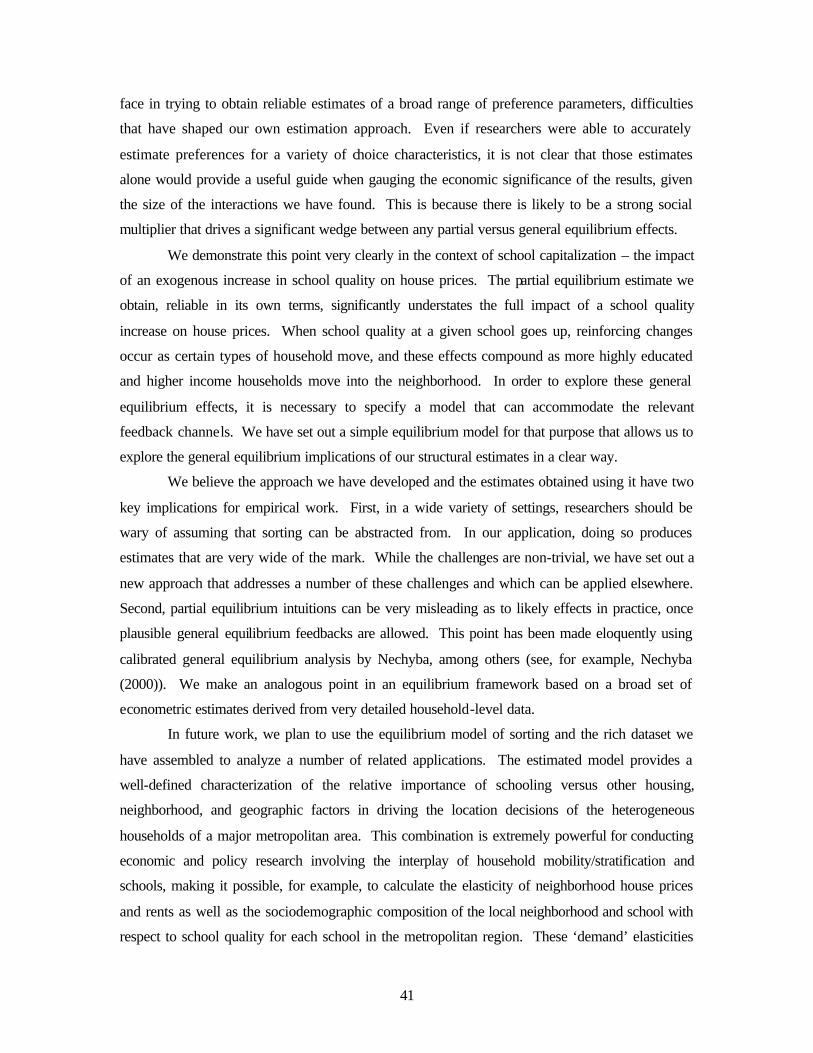
41

face in trying to obtain reliable estimates of a broad range of preference parameters, difficulties

that have shaped our own estimation approach. Even if researchers were able to accurately

estimate preferences for a variety of choice characteristics, it is not clear that those estimates

alone would provide a useful guide when gauging the economic significance of the results, given

the size of the interactions we have found. This is because there is likely to be a strong social

multiplier that drives a significant wedge between any partial versus general equilibrium effects.

We demonstrate this point very clearly in the context of school capitalization – the impact

of an exogenous increase in school quality on house prices. The partial equilibrium estimate we

obtain, reliable in its own terms, significantly understates the full impact of a school quality

increase on house prices. When school quality at a given school goes up, reinforcing changes

occur as certain types of household move, and these effects compound as more highly educated

and higher income households move into the neighborhood. In order to explore these general

equilibrium effects, it is necessary to specify a model that can accommodate the relevant

feedback channels. We have set out a simple equilibrium model for that purpose that allows us to

explore the general equilibrium implications of our structural estimates in a clear way.

We believe the approach we have developed and the estimates obtained using it have two

key implications for empirical work. First, in a wide variety of settings, researchers should be

wary of assuming that sorting can be abstracted from. In our application, doing so produces

estimates that are very wide of the mark. While the challenges are non-trivial, we have set out a

new approach that addresses a number of these challenges and which can be applied elsewhere.

Second, partial equilibrium intuitions can be very misleading as to likely effects in practice, once

plausible general equilibrium feedbacks are allowed. This point has been made eloquently using

calibrated general equilibrium analysis by Nechyba, among others (see, for example, Nechyba

(2000)). We make an analogous point in an equilibrium framework based on a broad set of

econometric estimates derived from very detailed household-level data.

In future work, we plan to use the equilibrium model of sorting and the rich dataset we

have assembled to analyze a number of related applications. The estimated model provides a

well-defined characterization of the relative importance of schooling versus other housing,

neighborhood, and geographic factors in driving the location decisions of the heterogeneous

households of a major metropolitan area. This combination is extremely powerful for conducting

economic and policy research involving the interplay of household mobility/stratification and

schools, making it possible, for example, to calculate the elasticity of neighborhood house prices

and rents as well as the sociodemographic composition of the local neighborhood and school with

respect to school quality for each school in the metropolitan region. These ‘demand’ elasticities

42

provide a series of measure of the competitiveness of a school’s local environment and can be

used to explore many aspects of the relations between household mobility and school

competition. Moreover, a slightly extended version of the model provides a way of calculating

the strength of preferences for school quality (on the basis of both observed and unobserved

characteristics) among the households that select into a particular school. This permits the

researcher to control directly for the non-random sorting of households across schools and school

districts which leads to a form of selection bias (often referred to as Tiebout bias in the local

public finance literature) in the estimation of education production functions, voting models, or

other models that condition implicitly on the set of households in a particular school or

jurisdiction.

REFERENCES Bajari, Patrick and Lanier Benkard, (2002), “Demand Estimation with Heterogeneous Consumers and Unobserved Product Characteristics: A Hedonic Approach,” unpublished manuscript, Stanford University. Bajari, Patrick, and Matthew Kahn (2001), “Why Do Blacks Live in Cities and Whites Live in Suburbs?” unpublished manuscript, Stanford University. Barrow, Lisa (2003), "School Choice through Relocation: Evidence from the Washington, D.C. area," Journal of Public Economics, forthcoming. Bayer, Patrick, (1999), An Empirical Analysis of the Equilibrium in the Education Market, Stanford University Dissertation. Bayer, Patrick, Robert McMillan, and Kim Rueben, (2002), “An Equilibrium Model of an Urban Housing Market: A Study of the Causes and Consequences of Residential Segregation,” unpublished manuscript, Yale University. Benabou, Roland, (1993), “The Workings of a City: Location, Education, and Production,” Quarterly Journal of Economics, 108(3), pp.619-652. Benabou, Roland, (1996), “Heterogeneity, Stratification, and Growth: Macroeconomic Implications of Community Structure and School Finance,” American Economic Review, Vol. 86, No. 3., pp. 584-609. Berry, Steven, (1994), “Estimating Discrete-Choice Models of Product Differentiation,” RAND Journal of Economics, Vol. 25, pp. 242-262. Berry, Steven, James Levinsohn, and Ariel Pakes, (1995), “Automobile Prices in Market Equilibrium,” Econometrica, Vol 63, pp. 841-890. Black, Sandra (1999) “Do Better Schools Matter? Parental Valuation of Elementary Education,” Quarterly Journal of Economics, May 1999.

43

Bogart, William T. and Brian A. Cromwell (2000) “How Much is a Neighborhood School Worth?” Journal of Urban Economics, 47, 280-305.

Brock, William and Steven Durlauf (2001), “Discrete Choice With Social Interactions” The Review of Economic Studies 68, No. 2, pp. 235-260.

Brock, William and Steven Durlauf (2001), “A Multinomial Choice Model of Neighborhood Effects, American Economic Review 92, No. 2, pp. 298-303.

Clapp, John M., and Stephen L. Ross, (2002) “Schools and Housing Markets: An Examination of School Segregation and Performance in Connecticut,’ unpublished manuscript, University of Connecticut. Ekeland, Ivar, James Heckman, and Lars Nesheim (2002), “Identification and Estimation of Hedonic Models,” Centre for Microdata Methods and Practice Working Paper CWP07/02. Epple, Dennis, (1987), “Hedonic Prices and Implicit Markets: Estimating Demand and Supply Functions for Differentiated Products,” Journal of Political Economy , 107: 645-81. Epple, D., R. Filimon, and T. Romer, (1984), “Equilibrium Among Local Jurisdictions: Towards an Integrated Approach of Voting and Residential Choice,” Journal of Public Economics, Vol. 24, pp. 281-304. Epple, D., R. Filimon, and T. Romer, (1993), “Existence of Voting and Housing Equilibrium in a System of Communities with Property Taxes,” Regional Science and Urban Economics, Vol. 23, pp. 585-610. Epple, Dennis and Holger Sieg, (1999), “Estimating Equilibrium Models of Local Jurisdictions,” Journal of Political Economy , Vol. 107, No. 4., pp. 645-681. Epple, Dennis and Richard Romano, (1998), “ Competition Between Private and Public Schools, Vouchers, and Peer Group Effects,” American Economic Review 88(1): 33-62. Fernandez, Raquel and Richard Rogerson, (1996), “Income Distribution, Communities, and the Quality of Public Education.” Quarterly Journal of Economics, Vol. 111, No. 1., pp. 135-164.

Fernandez, Raquel and Richard Rogerson, (2003), “Equity and Resources: An Analysis of Educational Finance Systems,” Journal of Political Economy, vol. 111, no. 4.

Figlio, David and Maurice Lucas (2000) “What’s in a Grade? School Report Cards and House Prices,” NBER Working Paper 8019, Cambridge, MA.

Hayes, Kathy J. and Lori L. Taylor, (1996) “Neighborhood School Characteristics: What Signals Quality to Homebuyer?” Economic Review: Federal Reserve Back of Dallas (4), 2-9. Heckman, James, Rosa Matzkin, and Lars Nesheim, (2003), “Simulation and Estimation of Hedonic Models,” unpublished manuscript, University of Chicago. Kane, Thomas, Douglas Staiger, and Gavin Samms, (2003) “School Accountability Ratings and Houise Values,” Brookings-Wharton Papers on Urban Affairs, forthcoming.

44

McFadden, Daniel, (1978), “Modeling the Choice of Residential Location,” in eds. Karlquist, A., et al., Spatia l Interaction Theory and Planning Models, Elsevier North-Holland, New York. Nechyba, Thomas J., (1997), “Existence of Equilibrium and Stratification in Local and Hierarchical Tiebout Economies with Property Taxes and Voting,” Economic Theory, Vol. 10, pp. 277-304. Nechyba, Thomas J., (1999), “School Finance Induced Migration and Stratification Patterns: the Impact of Private School Vouchers,” Journal of Public Economic Theory, Vol. 1. Nechyba, Thomas J., (2000), Mobility, Targeting and Private School Vouchers," American Economic Review 90(1), 130-46. Nechyba, Thomas J., and Robert P. Strauss, (1998), “Community Choice and Local Public Services: A Discrete Choice Approach,” Regional Science and Urban Economics, Vol. 28, pp. 51-73. Nesheim, Lars (2001), “Equilibrium Sorting of Heterogeneous Consumers Across Locations: Theory and Empirical Implications,” Ph. D. Dissertation, University of Chicago. Oates, Wallace “The Effects of Property Taxes and Local Public Spending on Property Values: An empirical Study of Tax Capitalization and the Tiebout Hypothesis,” Journal of Political Economy 77(6): 957-71. Quigley, John M., (1985), “Consumer Choice of Dwelling, Neighborhood, and Public Services,” Regional Science and Urban Economics, Vol. 15(1). Rosen, Sherwin, (1974), “Hedonic Prices and Implicit Markets: Product Differentiation in Pure Competition,” Journal of Political Economy , 82: 34-55. Rothstein, Jesse, (2002), “Good Principals or Good Peers: Parental Valuation of School Characteristics, Tiebout Equilibrium, and the Incentive Effects of Competition Among Jurisdictions”. mimeo, University of California, Berkeley. Tiebout, Charles M., (1956), “A Pure Theory of Local Expenditures,” Journal of Political Economy, 64: 416-424. Tinbergen, Jan (1956), “On the Theory of Income Distribution,” Weltwirtschaftliches Archiv 77: 155-73.

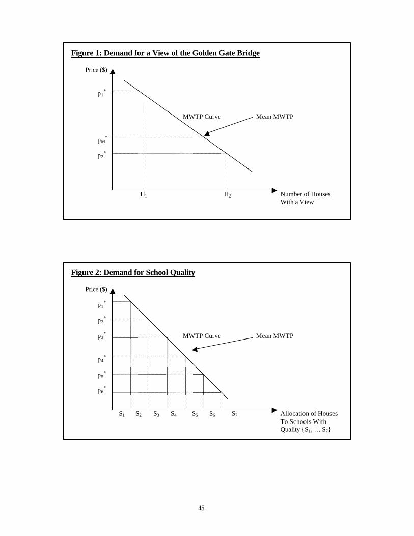
45

Figure 1: Demand for a View of the Golden Gate Bridge

Price ($) p1

* MWTP Curve Mean MWTP pM

* p2

*

H1 H2 Number of Houses With a View

Figure 2: Demand for School Quality

Price ($) p1

*

p2*

p3

* MWTP Curve Mean MWTP p4

* p5

* p6

*

S1 S2 S3 S4 S5 S6 S7 Allocation of Houses To Schools With Quality S1, … S7

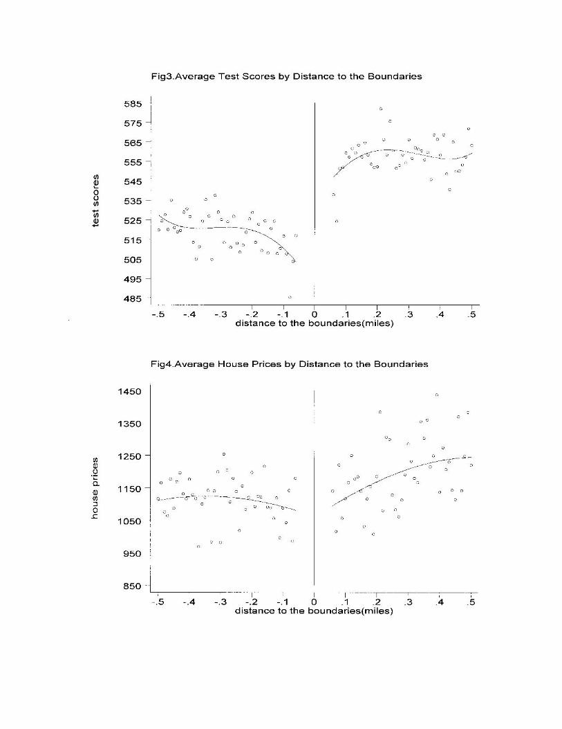
44

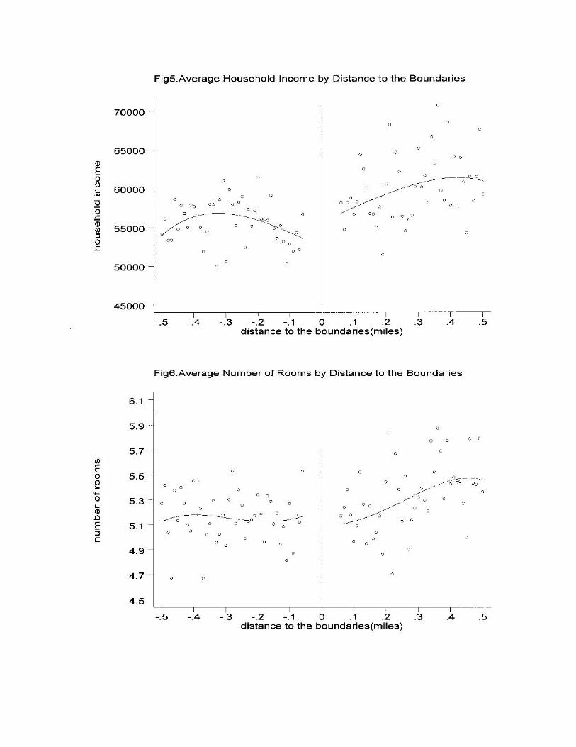
45

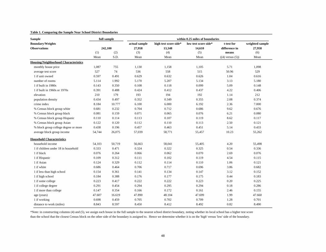
Table 1. Comparing the Sample Near School District Boundaries

Sample full sample

Boundary/Weights actual sample high test score side* low test score side* t-test for weighted sample

Observations 27,958 13,348 14,610 difference in 27,958(1) (2) (3) (4) (5) means (6)

Mean S.D. Mean Mean Mean ((4) versus (5)) Mean

Housing/Neighborhood Characteristics

monthly house price 1,087 755 1,130 1,158 1,105 5.71 1,098

average test score 527 74 536 558 515 50.96 529

1 if unit owned 0.597 0.491 0.629 0.632 0.626 1.04 0.616

number of rooms 5.114 1.992 5.170 5.207 5.134 3.13 5.180

1 if built in 1980s 0.143 0.350 0.108 0.118 0.099 5.09 0.148

1 if built in 1960s or 1970s 0.391 0.488 0.424 0.412 0.437 4.22 0.406

elevation 210 179 193 194 192 1.14 212

population density 0.434 0.497 0.352 0.349 0.355 2.08 0.374

crime index 8.184 10.777 6.100 6.000 6.192 2.36 7.000

% Census block group white 0.681 0.232 0.704 0.712 0.686 9.62 0.676

% Census block group black 0.081 0.159 0.071 0.065 0.076 6.21 0.080

% Census block group Hispanic 0.110 0.114 0.113 0.107 0.119 8.62 0.117

% Census block group Asian 0.122 0.120 0.112 0.110 0.113 2.50 0.121

% block group college degree or more 0.438 0.196 0.457 0.463 0.451 5.14 0.433

average block group income 54,744 26,075 57,039 58,771 55,457 10.23 55,262

Household Characteristics

household income 54,103 50,719 56,663 58,041 55,405 4.20 55,498

1 if children under 18 in household 0.333 0.471 0.324 0.322 0.325 0.54 0.336

1 if black 0.076 0.264 0.066 0.062 0.070 2.69 0.076

1 if Hispanic 0.109 0.312 0.111 0.102 0.119 4.54 0.115

1 if Asian 0.124 0.329 0.112 0.114 0.110 1.06 0.121

1 if white 0.686 0.464 0.706 0.717 0.696 3.86 0.682

1 if less than high school 0.154 0.361 0.141 0.134 0.147 3.12 0.152

1 if high school 0.184 0.388 0.176 0.177 0.175 0.44 0.183

1 if some college 0.223 0.417 0.222 0.222 0.223 0.20 0.225

1 if college degree 0.291 0.454 0.294 0.295 0.294 0.18 0.286

1 if more than college 0.147 0.354 0.166 0.172 0.161 2.46 0.155

age (years) 47.607 16.619 47.890 48.104 47.699 1.99 47.660

1 if working 0.698 0.459 0.705 0.702 0.709 1.28 0.701

distance to work (miles) 8.843 8.597 8.450 8.412 8.492 0.82 8.490

*Note: in constructing columns (4) and (5), we assign each house in the full sample to the nearest school district boundary, noting whether its local school has a higher test score

than the school that the closest Census block on the other side of the boundary is assigned to. Hence we determine whether it is on the 'high' versus 'low' side of the boundary.

within 0.25 miles of boundaries

242,100

48

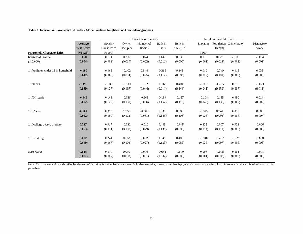
Average Monthly Owner Number of Built in Built in Elevation Population Crime Index Distance to

Test Score House Price Occupied Rooms 1980s 1960-1979 Density Work

Household Characteristics (+1 s.d.) (/1000) (/100)

household income 0.050 0.121 0.305 0.074 0.142 0.038 0.016 0.028 -0.001 -0.004

(/10,000) (0.004) (0.003) (0.010) (0.002) (0.011) (0.009) (0.001) (0.013) (0.001) (0.001)

1 if children under 18 in household -0.190 0.063 -0.102 0.544 -0.316 0.146 0.010 -0.740 0.015 0.036

(0.047) (0.065) (0.094) (0.025) (0.112) (0.083) (0.022) (0.101) (0.005) (0.005)

1 if black -1.395 -0.941 -0.510 0.152 0.004 0.401 -0.062 -1.285 0.110 -0.023

(0.080) (0.127) (0.167) (0.044) (0.211) (0.144) (0.041) (0.159) (0.007) (0.011)

1 if Hispanic -0.642 0.168 -0.036 -0.268 -0.180 -0.157 -0.104 -0.155 0.050 0.014

(0.072) (0.122) (0.130) (0.036) (0.164) (0.115) (0.040) (0.136) (0.007) (0.007)

1 if Asian -0.167 0.315 1.765 -0.503 1.037 0.686 -0.015 0.941 0.030 0.003

(0.062) (0.080) (0.122) (0.031) (0.145) (0.108) (0.028) (0.095) (0.006) (0.007)

1 if college degree or more 0.787 0.917 -0.032 -0.012 0.489 -0.045 0.225 -0.007 0.031 -0.006

(0.053) (0.071) (0.108) (0.029) (0.135) (0.093) (0.024) (0.111) (0.006) (0.006)

1 if working 0.007 0.244 0.563 0.032 0.641 0.406 -0.048 -0.437 -0.027 -0.858

(0.049) (0.067) (0.103) (0.027) (0.125) (0.086) (0.025) (0.097) (0.005) (0.008)

age (years) 0.015 0.010 0.090 0.004 -0.034 -0.009 0.003 -0.006 0.001 -0.001

(0.001) (0.002) (0.003) (0.001) (0.004) (0.003) (0.001) (0.003) (0.000) (0.000)

Note: The parameters shown describe the elements of the utility function that interact household characteristics, shown in row headings, with choice characteristics, shown in column headings. Standard errors are in parentheses.

Neighborhood Attributes

Table 2. Interaction Parameter Estimates - Model Without Neighborhood Sociodemographics

House Characteristics

49

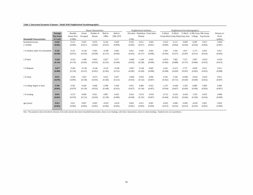
Average Monthly Owner Number of Built in Built in Elevation Population Crime Index % Block % Block % Block % Blk Group Blk Group Distance to

Test Score House Price Occupied Rooms 1980s 1960-1979 Density Group BlackGroup HispGroup Asian College Avg Income Work

Household Characteristics (+1 s.d.) (/1000) (/100) (miles)

household income 0.020 0.121 0.303 0.076 0.144 0.028 0.010 0.011 -0.001 -0.223 0.113 -0.009 0.385 0.012 -0.004

(+10,000) (0.005) (0.004) (0.011) (0.003) (0.012) (0.009) (0.002) (0.017) (0.001) (0.060) (0.064) (0.039) (0.034) (0.002) (0.001)

1 if children under 18 in household 0.102 0.231 -0.238 0.582 -0.399 0.095 0.051 -0.947 0.002 1.594 2.294 1.857 -2.171 0.055 0.027

(0.058) (0.075) (0.103) (0.028) (0.122) (0.092) (0.025) (0.127) (0.006) (0.416) (0.527) (0.387) (0.331) (0.016) (0.005)

1 if black -0.282 0.143 -1.006 0.002 0.027 0.577 -0.068 -1.106 0.045 14.874 7.082 7.371 2.607 -0.023 -0.010

(0.116) (0.170) (0.205) (0.053) (0.253) (0.184) (0.052) (0.228) (0.009) (0.560) (0.888) (0.747) (0.680) (0.035) (0.013)

1 if Hispanic -0.077 0.204 -0.138 -0.246 -0.147 -0.248 -0.067 -0.128 0.005 4.435 12.471 2.757 0.830 0.011 0.012

(0.089) (0.139) (0.147) (0.041) (0.185) (0.131) (0.045) (0.169) (0.008) (0.568) (0.620) (0.587) (0.492) (0.022) (0.008)

1 if Asian 0.072 0.558 1.633 -0.571 0.612 0.457 -0.006 -0.053 0.006 4.236 3.330 14.060 -0.016 -0.022 0.012

(0.078) (0.095) (0.138) (0.035) (0.166) (0.123) (0.033) (0.132) (0.007) (0.562) (0.721) (0.429) (0.449) (0.022) (0.007)

1 if college degree or more 0.200 0.501 0.428 0.006 0.588 0.106 0.031 0.486 0.022 1.279 -0.638 -1.935 8.986 0.009 0.009

(0.065) (0.079) (0.118) (0.032) (0.148) (0.101) (0.027) (0.134) (0.007) (0.504) (0.607) (0.450) (0.366) (0.020) (0.007)

1 if working 0.093 0.272 0.604 0.021 0.897 0.425 0.023 -0.515 -0.019 -0.712 -0.335 -0.434 -1.931 0.033 -0.896

(0.062) (0.074) (0.113) (0.030) (0.138) (0.096) (0.028) (0.125) (0.007) (0.444) (0.563) (0.436) (0.350) (0.016) (0.009)

age (years) 0.013 0.011 0.097 0.003 -0.033 -0.010 0.003 -0.011 0.001 -0.022 -0.085 -0.005 -0.018 0.001 -0.001

(0.002) (0.002) (0.003) (0.001) (0.004) (0.003) (0.001) (0.003) (0.000) (0.013) (0.016) (0.013) (0.010) (0.001) (0.000)

Note: The parameters shown describe the elements of the utility function that interact household characteristics, shown in row headings, with choice characteristics, shown in column headings. Standard errors are in parentheses.

Table 3. Interaction Parameter Estimates - Model With Neighborhood Sociodemographics

House Characteristics Neighborhood Attributes Neighborhood Sociodemographics

50

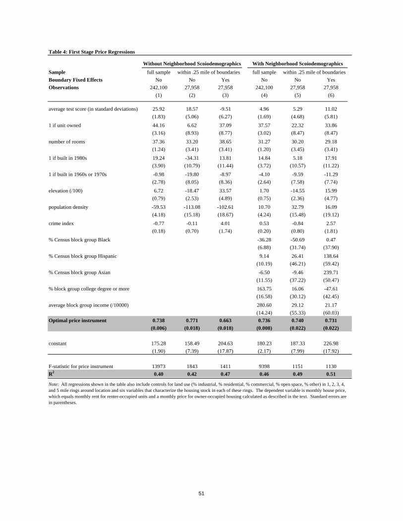
Table 4: First Stage Price Regressions

Sample

Boundary Fixed Effects

Observations

average test score (in standard deviations)

1 if unit owned

number of rooms

1 if built in 1980s

1 if built in 1960s or 1970s

elevation (/100)

population density

crime index

% Census block group Black

% Census block group Hispanic

% Census block group Asian

% block group college degree or more

average block group income (/10000)

Optimal price instrument

constant

F-statistic for price instrument

R2 0.49 0.51

13973 1843

0.40 0.42 0.47 0.46

1411 9398

187.33 226.98

(7.99) (17.92)

1151 1130

(1.90) (7.39) (17.87) (2.17)

175.28 158.49 204.63 180.23

0.740 0.731

(0.006) (0.018) (0.018) (0.008) (0.022) (0.022)

0.738 0.771 0.663 0.736

No No

29.12

(55.33)

16.06

(30.12)(16.58)

280.60

Yes

21.17

(60.03)

239.71

(50.47)

-47.61

(42.45)

0.47

(37.90)

138.64

(59.42)

16.09

(19.12)

2.57

(1.81)

11.02

(5.81)

15.99

(4.77)

33.86

(8.47)

29.18

(3.41)

17.91

(11.22)

-11.29

(7.74)

-9.46

(37.22)

-50.69

(31.74)

26.41

(46.21)

32.79

(15.48)

5.29

(4.68)

-14.55

(2.36)

-0.84

(0.80)

(10.19)

-6.50

(11.55)

163.75

(0.20)

-36.28

(6.88)

9.14

(1.69)

1.70

(0.75)

10.70

(3.72)

-4.10

(2.64)

4.01

(4.24)

0.53

(3.02)

31.27

(1.20)

14.84

38.65

4.96

(4.89)

-102.61

(18.67)

(8.36)

-9.51

(6.27)

33.57

(3.41)

13.81

(0.70)

27,95827,958

(5.06)

-18.47

(1.74)

(15.18)

-0.11

37.09

(8.77)

(2.53)

-113.08

(8.05)

(11.44)

-8.97

(14.24)

22.32

(8.47)

30.20

(3.45)

5.18

(10.57)

-9.59

(7.58)

37.57

(4.18)

-0.77

(0.18)

6.62

(8.93)

33.20

(3.41)

-34.31

(10.79)

-19.80

-59.53

44.16

(3.16)

37.36

(1.24)

19.24

(3.90)

-0.98

Without Neighborhood Scoiodemographics

(1.83)

242,100

18.57

within .25 mile of boundaries

No No Yes

(1) (2)

With Neighborhood Scoiodemographics

full sample

Note: All regressions shown in the table also include controls for land use (% industrial, % residential, % commercial, % open space, % other) in 1, 2, 3, 4, and 5 mile rings around location and six variables that characterize the housing stock in each of these rings. The dependent variable is monthly house price, which equals monthly rent for renter-occupied units and a monthly price for owner-occupied housing calculated as described in the text. Standard errors are in parentheses.

full sample

27,958 27,958242,100

within .25 mile of boundaries

(2.78)

25.92

6.72

(0.79)

(3) (4) (5) (6)

51

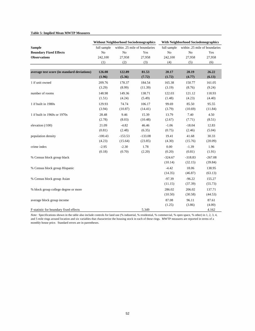
Table 5: Implied Mean MWTP Measures

Sample

Boundary Fized Effects

Observations

average test score (in standard deviations)

1 if unit owned

number of rooms

1 if built in 1980s

1 if built in 1960s or 1970s

elevation (/100)

population density

crime index

% Census block group black

% Census block group Hispanic

% Census block group Asian

% block group college degree or more

average block group income

F-statistic for boundary fixed effects

Note: Specifications shown in the table also include controls for land use (% industrial, % residential, % commercial, % open space, % other) in 1, 2, 3, 4, and 5 mile rings around location and six variables that characterize the housing stock in each of these rings. MWTP measures are reported in terms of a monthly house price. Standard errors are in parentheses.

Without Neighborhood Sociodemographics With Neighborhood Sociodemographics

full sample full samplewithin .25 mile of boundaries within .25 mile of boundaries

27,958 27,958

209.76

(3.29)

184.54

(11.39)

242,100 27,958 27,958 242,100

28.48

(2.78)

126.08

(1.96)

148.98

(1.51)

129.93

(3.94)

21.09

(0.81)

-100.43

(4.23)

-2.95

(0.18)

178.37

(8.99)

149.36

(4.24)

74.74

(10.87)

9.46

(8.03)

122.89

(5.36)

-4.82

(2.48)

-153.53

(15.64)

-2.30

(0.70)

15.39

(10.48)

81.53

(7.72)

138.71

(5.49)

106.17

(14.41)

46.46

(6.35)

-133.08

(23.85)

1.78

(2.20)

165.38

(3.19)

122.03

(1.48)

99.69

(3.79)

13.79

(2.67)

20.17

(1.72)

-1.06

(0.75)

19.41

(4.30)

0.00

(0.20)

-324.67

(10.14)

-4.42

(14.35)

-97.39

(11.15)

286.02

(10.50)

87.08(1.25)

150.77

(8.76)

121.12

(4.23)

85.50

(10.69)

7.40

(7.71)

20.19

(4.77)

-18.04

(2.46)

41.68

(15.76)

-1.39

(0.81)

-318.83

(32.15)

18.06

(46.87)

-96.22

(37.39)

206.02

(30.58)

96.11(3.86)

161.05

(9.24)

118.93

(4.40)

95.55

(11.84)

4.50

(8.51)

26.22

(6.13)

12.83

(5.04)

30.33

(20.09)

1.96

(1.91)

-267.08

(39.84)

138.95

(63.13)

No No Yes No

5.349 4.162

No Yes

87.61(4.00)

155.27

(55.73)

137.71

(44.53)

(5) (6)(1) (2) (3) (4)

52

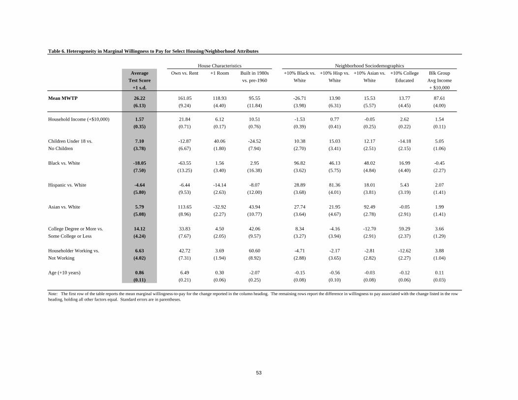
Average Own vs. Rent +1 Room Built in 1980s +10% Black vs. +10% Hisp vs. +10% Asian vs. +10% College Blk Group

Test Score vs. pre-1960 White White White Educated Avg Income

+1 s.d. + $10,000

Mean MWTP 26.22 161.05 118.93 95.55 -26.71 13.90 15.53 13.77 87.61

(6.13) (9.24) (4.40) (11.84) (3.98) (6.31) (5.57) (4.45) (4.00)

Household Income (+$10,000) 1.57 21.84 6.12 10.51 -1.53 0.77 -0.05 2.62 1.54

(0.35) (0.71) (0.17) (0.76) (0.39) (0.41) (0.25) (0.22) (0.11)

Children Under 18 vs. 7.10 -12.87 40.06 -24.52 10.38 15.03 12.17 -14.18 5.05

No Children (3.78) (6.67) (1.80) (7.94) (2.70) (3.41) (2.51) (2.15) (1.06)

Black vs. White -18.05 -63.55 1.56 2.95 96.82 46.13 48.02 16.99 -0.45

(7.50) (13.25) (3.40) (16.38) (3.62) (5.75) (4.84) (4.40) (2.27)

Hispanic vs. White -4.64 -6.44 -14.14 -8.07 28.89 81.36 18.01 5.43 2.07

(5.80) (9.53) (2.63) (12.00) (3.68) (4.01) (3.81) (3.19) (1.41)

Asian vs. White 5.79 113.65 -32.92 43.94 27.74 21.95 92.49 -0.05 1.99

(5.08) (8.96) (2.27) (10.77) (3.64) (4.67) (2.78) (2.91) (1.41)

College Degree or More vs. 14.12 33.83 4.50 42.06 8.34 -4.16 -12.70 59.29 3.66

Some College or Less (4.24) (7.67) (2.05) (9.57) (3.27) (3.94) (2.91) (2.37) (1.29)

Householder Working vs. 6.63 42.72 3.69 60.60 -4.71 -2.17 -2.81 -12.62 3.88

Not Working (4.02) (7.31) (1.94) (8.92) (2.88) (3.65) (2.82) (2.27) (1.04)

Age (+10 years) 0.86 6.49 0.30 -2.07 -0.15 -0.56 -0.03 -0.12 0.11

(0.11) (0.21) (0.06) (0.25) (0.08) (0.10) (0.08) (0.06) (0.03)

Note: The first row of the table reports the mean marginal willingness-to-pay for the change reported in the column heading. The remaining rows report the difference in willingness to pay associated with the change listed in the row heading, holding all other factors equal. Standard errors are in parentheses.

Table 6. Heterogeneity in Marginal Willingness to Pay for Select Housing/Neighborhood Attributes

House Characteristics Neighborhood Sociodemographics

53

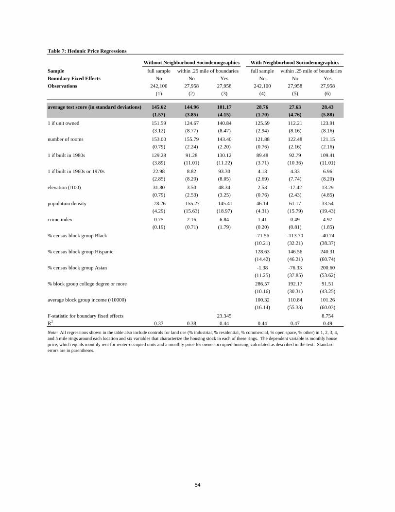
Table 7: Hedonic Price Regressions

Sample

Boundary Fixed Effects

Observations

average test score (in standard deviations)

1 if unit owned

number of rooms

1 if built in 1980s

1 if built in 1960s or 1970s

elevation (/100)

population density

crime index

% census block group Black

% census block group Hispanic

% census block group Asian

% block group college degree or more

average block group income (/10000)

F-statistic for boundary fixed effects

R2

Note: All regressions shown in the table also include controls for land use (% industrial, % residential, % commercial, % open space, % other) in 1, 2, 3, 4, and 5 mile rings around each location and six variables that characterize the housing stock in each of these rings. The dependent variable is monthly house price, which equals monthly rent for renter-occupied units and a monthly price for owner-occupied housing, calculated as described in the text. Standard errors are in parentheses.

full sample

27,958 27,958242,100

within .25 mile of boundaries

(2.85)

145.62

31.80

(0.79)

With Neighborhood Sociodemographics

full sample

Without Neighborhood Sociodemographics

(1.57)

242,100

144.96

within .25 mile of boundaries

No No Yes

(1) (2)

-78.26

151.59

(3.12)

153.00

(0.79)

129.28

(3.89)

22.98

(4.29)

0.75

(0.19)

124.67

(8.77)

155.79

(2.24)

91.28

(11.01)

8.82

(16.14)

112.21

(8.16)

122.48

(2.16)

92.79

(10.36)

4.33

(7.74)

125.59

(2.53)

-155.27

(8.20)

(11.22)

93.30

(0.71)

27,95827,958

(3.85)

3.50

(1.79)

(15.63)

2.16

140.84

(8.47)

28.76

(3.25)

-145.41

(18.97)

(8.05)

101.17

(4.15)

48.34

(2.20)

130.12

6.84

(4.31)

1.41

(2.94)

121.88

(0.76)

89.48

143.40

(1.70)

2.53

(0.76)

46.14

(3.71)

4.13

(2.69)

(0.20)

-71.56

(10.21)

128.63

(14.42)

-1.38

(11.25)

286.57

(10.16)

100.32

27.63

(4.76)

-17.42

(2.43)

61.17

(15.79)

0.49

(0.81)

-113.70

(32.21)

146.56

(46.21)

-76.33

(37.85)

192.17

(30.31)

110.84

(55.33)

123.91

(8.16)

121.15

(2.16)

109.41

(11.01)

6.96

(8.20)

28.43

(5.88)

13.29

(4.85)

33.54

(19.43)

4.97

(1.85)

-40.74

(38.37)

240.31

(60.74)

No No Yes

8.754

101.26

(60.03)

200.60

(53.62)

91.51

(43.25)

0.47 0.49

23.345

0.37 0.38 0.44 0.44

(3) (4) (5) (6)

54

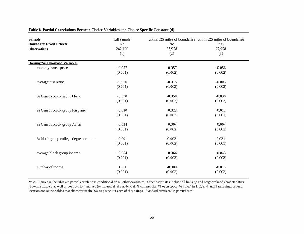
Table 8. Partial Correlations Between Choice Variables and Choice Specific Constant (δδ)

SampleBoundary Fixed EffectsObservations

Housing/Neighborhood Variablesmonthly house price

average test score

% Census block group black

% Census block group Hispanic

% Census block group Asian

% block group college degree or more

average block group income

number of rooms

Note: Figures in the table are partial correlations conditional on all other covariates. Other covariates include all housing and neighbrohood characteristics shown in Table 2 as well as controls for land use (% industrial, % residential, % commercial, % open space, % other) in 1, 2, 3, 4, and 5 mile rings around location and six variables that characterize the housing stock in each of these rings. Standard errors are in parentheses.

242,100 27,958 27,958

-0.057(0.001)

-0.016(0.001)

full sample within .25 miles of boundaries within .25 miles of boundariesYesNoNo

-0.078(0.001)

-0.030

(0.001)

(0.001)

-0.034(0.001)

-0.054(0.001)

0.001(0.001)

-0.057(0.002)

-0.015(0.002)

-0.050(0.002)

(0.002)

(0.002)

-0.023(0.002)

-0.004

-0.066(0.002)

-0.009(0.002)

-0.056(0.002)

-0.003(0.002)

-0.038(0.002)

-0.012(0.001)

-0.045(0.002)

-0.004(0.001)

0.031

-0.013(0.002)

(1) (2) (3)

0.003-0.001(0.001)

55

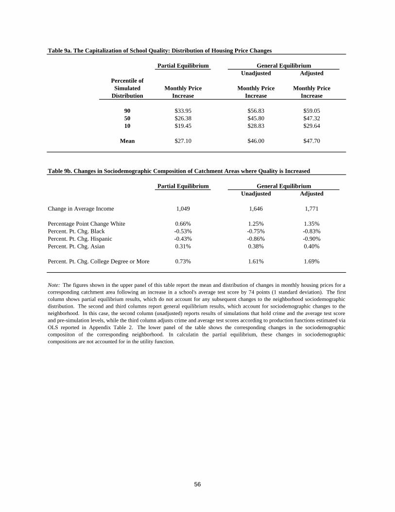
Table 9a. The Capitalization of School Quality: Distribution of Housing Price Changes

Partial EquilibriumUnadjusted Adjusted

Percentile ofSimulated Monthly Price Monthly Price Monthly Price

Distribution Increase Increase Increase

90 $33.95 $56.83 $59.0550 $26.38 $45.80 $47.3210 $19.45 $28.83 $29.64

Mean $27.10 $46.00 $47.70

Table 9b. Changes in Sociodemographic Composition of Catchment Areas where Quality is Increased

Partial EquilibriumUnadjusted Adjusted

Change in Average Income 1,049 1,646 1,771

Percentage Point Change White 0.66% 1.25% 1.35%Percent. Pt. Chg. Black -0.53% -0.75% -0.83%Percent. Pt. Chg. Hispanic -0.43% -0.86% -0.90%Percent. Pt. Chg. Asian 0.31% 0.38% 0.40%

Percent. Pt. Chg. College Degree or More 0.73% 1.61% 1.69%

General Equilibrium

Note: The figures shown in the upper panel of this table report the mean and distribution of changes in monthly housing prices for acorresponding catchment area following an increase in a school's average test score by 74 points (1 standard deviation). The firstcolumn shows partial equilibrium results, which do not account for any subsequent changes to the neighborhood sociodemographicdistribution. The second and third columns report general equilibrium results, which account for sociodemographic changes to theneighborhood. In this case, the second column (unadjusted) reports results of simulations that hold crime and the average test scoreand pre-simulation levels, while the third column adjusts crime and average test scores according to production functions estimated viaOLS reported in Appendix Table 2. The lower panel of the table shows the corresponding changes in the sociodemographiccomposiiton of the corresponding neighborhood. In calculatin the partial equilibrium, these changes in sociodemographiccompositions are not accounted for in the utility function.

General Equilibrium

56

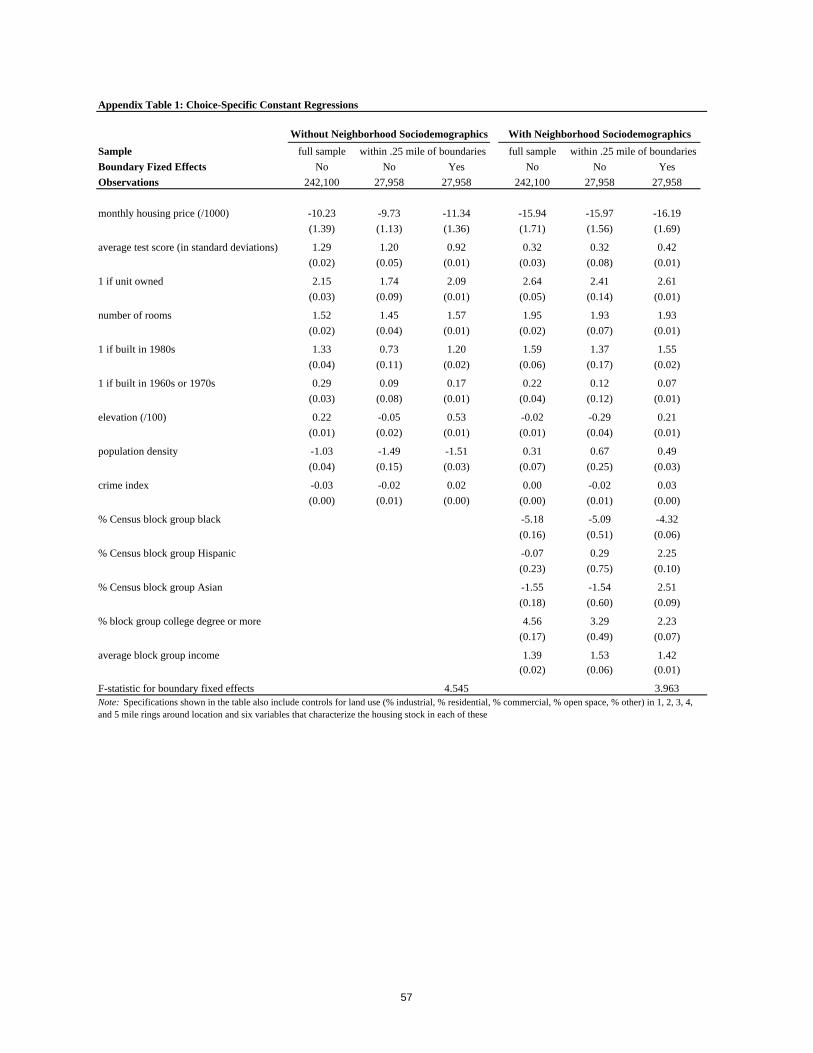
Appendix Table 1: Choice-Specific Constant Regressions

Sample

Boundary Fized Effects

Observations

monthly housing price (/1000)

average test score (in standard deviations)

1 if unit owned

number of rooms

1 if built in 1980s

1 if built in 1960s or 1970s

elevation (/100)

population density

crime index

% Census block group black

% Census block group Hispanic

% Census block group Asian

% block group college degree or more

average block group income

F-statistic for boundary fixed effects

-15.97

(1.56) (1.69)

-16.19-11.34

(1.36) (1.71)

-15.94-10.23

(1.39) (1.13)

-9.73

4.545 3.963

No Yes

1.42(0.01)

2.51

(0.09)

2.23

(0.07)

No No Yes No

-4.32

(0.06)

2.25

(0.10)

0.49

(0.03)

0.03

(0.00)

0.42

(0.01)

0.21

(0.01)

1.53(0.06)

2.61

(0.01)

1.93

(0.01)

1.55

(0.02)

0.07

(0.01)

-1.54

(0.60)

3.29

(0.49)

-5.09

(0.51)

0.29

(0.75)

0.67

(0.25)

-0.02

(0.01)

0.32

(0.08)

-0.29

(0.04)

1.39(0.02)

2.41

(0.14)

1.93

(0.07)

1.37

(0.17)

0.12

(0.12)

-1.55

(0.18)

4.56

(0.17)

-5.18

(0.16)

-0.07

(0.23)

0.31

(0.07)

0.00

(0.00)

0.32

(0.03)

-0.02

(0.01)

0.02

(0.00)

2.64

(0.05)

1.95

(0.02)

1.59

(0.06)

0.22

(0.04)

0.53

(0.01)

-1.51

(0.03)

0.17

(0.01)

0.92

(0.01)

1.57

(0.01)

1.20

(0.02)

-1.49

(0.15)

-0.02

(0.01)

1.20

(0.05)

-0.05

(0.02)

-0.03

(0.00)

1.74

(0.09)

1.45

(0.04)

0.73

(0.11)

0.09

(0.08)

0.22

(0.01)

-1.03

(0.04)

0.29

(0.03)

1.29

(0.02)

1.52

(0.02)

1.33

(0.04)

27,958 27,958

2.15

(0.03)

2.09

(0.01)

242,100 27,958 27,958 242,100

Without Neighborhood Sociodemographics With Neighborhood Sociodemographics

full sample full samplewithin .25 mile of boundaries within .25 mile of boundaries

Note: Specifications shown in the table also include controls for land use (% industrial, % residential, % commercial, % open space, % other) in 1, 2, 3, 4, and 5 mile rings around location and six variables that characterize the housing stock in each of these

57

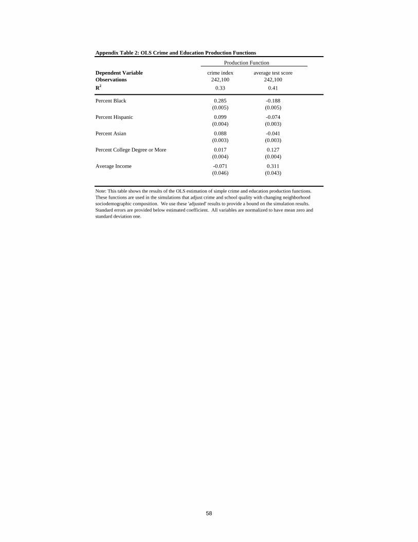
Appendix Table 2: OLS Crime and Education Production Functions

Production Function

Dependent Variable crime index average test scoreObservations 242,100 242,100

R2 0.33 0.41

Percent Black 0.285 -0.188(0.005) (0.005)

Percent Hispanic 0.099 -0.074(0.004) (0.003)

Percent Asian 0.088 -0.041(0.003) (0.003)

Percent College Degree or More 0.017 0.127(0.004) (0.004)

Average Income -0.071 0.311(0.046) (0.043)

Note: This table shows the results of the OLS estimation of simple crime and education production functions. These functions are used in the simulations that adjust crime and school quality with changing neighborhood sociodemographic composition. We use these 'adjusted' results to provide a bound on the simulation results. Standard errors are provided below estimated coefficient. All variables are normalized to have mean zero and standard deviation one.

58

59

Technical Appendix

Introduction

This appendix supplements the description of the estimation procedure provided in the main text

of the paper. To avoid repetition, this document assumes that the reader has read the discussion in the

main text. In that discussion, we abstract from many of the issues discussed here, which are of a more

technical nature, in order to maintain the focus on issues associated with the identification of preferences

for schools and neighbors and on relating our approach to other approaches that appear in the labor and

public, rather than the IO, literatures.

Defining the Choice Set

In order to provide a coherent discussion of the properties of the estimator, it is helpful to provide

an exact characterization of the choice problem – in particular, whether it should literally be viewed as the

choice of a single residence from the full census of residences available in the Bay Area housing market

or as the choice of a representative housing type. The assumption that the underlying individual

component of the error term εε ih is distributed according to the extreme value distribution allows us some

flexibility in terms of the interpretation of the underlying choice problem. Given that the IIA property

holds for each individual, the econometrician has some flexibility in using a subset of the full set of

alternatives in estimating the model. As it turns out, however, it is much more straightforward to develop

the equilibrium properties of our model as well as the asymptotic properties of the estimator if we assume

that the full census of available houses can be characterized by a smaller set of representative housing

types.

Accordingly, we characterize the economic environment as follows: The model is estimated on

data drawn from a single, large metropolitan area. The complete metropolitan area housing market

consists of a total of I individuals who must choose from H distinct types of housing, with H assumed to

be less than I. Each individual i is characterized by a set of characteristics Zi and a set of idiosyncratic

preferences εih defined over the full set of distinct housing alternatives, and identically and

independently distributed across choices according to the extreme value distribution. Households are

assumed to follow the model’s decision rule at the true parameter vector. Each distinct housing type k is

characterized by the set of characteristics Xk, ξk. The Xk, ξk vectors are assumed to be exchangeable

draws from some larger population of possible house types.

We do not observe the full census of households and houses in the metropolitan area, but instead

observe a random sample of households SI of size N and their corresponding houses SH. We assume that

N is large relative to H so that the market shares for the H distinct types of housing are given by nH/N,

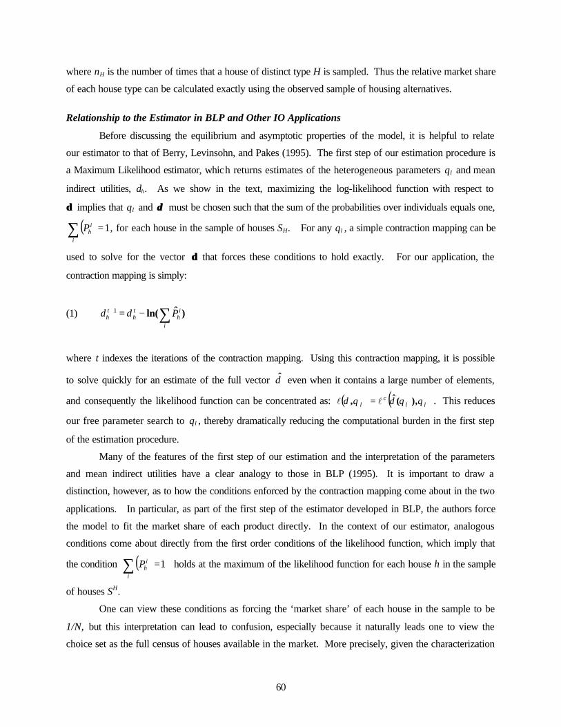
60

where nH is the number of times that a house of distinct type H is sampled. Thus the relative market share

of each house type can be calculated exactly using the observed sample of housing alternatives.

Relationship to the Estimator in BLP and Other IO Applications

Before discussing the equilibrium and asymptotic properties of the model, it is helpful to relate

our estimator to that of Berry, Levinsohn, and Pakes (1995). The first step of our estimation procedure is

a Maximum Likelihood estimator, which returns estimates of the heterogeneous parameters θλ and mean

indirect utilities, δh. As we show in the text, maximizing the log-likelihood function with respect to

δ δ implies that θλ and δδ must be chosen such that the sum of the probabilities over individuals equals one,

( ) 1=∑i

ihP , for each house in the sample of houses SH. For any θλ, a simple contraction mapping can be

used to solve for the vector δδ that forces these conditions to hold exactly. For our application, the

contraction mapping is simply:

(1) )ˆln(∑−=+

i

ih

th

th Pδδ 1

where t indexes the iterations of the contraction mapping. Using this contraction mapping, it is possible

to solve quickly for an estimate of the full vector δ even when it contains a large number of elements,

and consequently the likelihood function can be concentrated as: ( ) ( )λλλ θθδθδ ),(ˆ, cll = . This reduces

our free parameter search to θλ, thereby dramatically reducing the computational burden in the first step

of the estimation procedure.

Many of the features of the first step of our estimation and the interpretation of the parameters

and mean indirect utilities have a clear analogy to those in BLP (1995). It is important to draw a

distinction, however, as to how the conditions enforced by the contraction mapping come about in the two

applications. In particular, as part of the first step of the estimator developed in BLP, the authors force

the model to fit the market share of each product directly. In the context of our estimator, analogous

conditions come about directly from the first order conditions of the likelihood function, which imply that

the condition ( ) 1=∑i

ihP holds at the maximum of the likelihood function for each house h in the sample

of houses SH.

One can view these conditions as forcing the ‘market share’ of each house in the sample to be

1/N, but this interpretation can lead to confusion, especially because it naturally leads one to view the

choice set as the full census of houses available in the market. More precisely, given the characterization

61

of the data generating process above, these conditions force the market share of each distinct house type

H to be nH/N, which is its true market share. In this way, an analogy with IO applications is fairly direct

under our preferred interpretation of the choice problem; and the fact the conditions wind up as

( ) 1=∑i

ihP simply reflects the fact that these sums are taken over the houses in the sample, not distinct

house types .

Sampling

An important aspect of the underlying IIA property for each individual is that we can estimate the

model using only a sample of the alternatives not selected by the individual, following McFadden (1978).

This permits estimation despite having many alternatives – i.e., many distinct house types. The particular

procedure that we use is as follows. Using the sample of households SI and their corresponding houses SH

from the full data set, for each household i observed in this sample, we construct a subset SiH that consists

of the household’s chosen house and a random sample of the remaining alternatives in SH. In practice,

because we estimate a mean indirect utility for each house observed in the sample, the precision of the

estimation procedure increases greatly if we ensure that each alternative appears in the choice set of the

same number of households. To this end, we employ the following random sampling procedure: Starting

with the assignment of each household’s chosen house, we assign each household a first additional (not

chosen) alternative by randomly re-shuffling the full set of houses across households. We then repeat this

random re-shuffling of houses as many times as is necessary to generate the desired size of the sample of

additional (not chosen) alternatives. In this way, with an additional random draw for each household, we

ensure that each alternative is sampled exactly once.

In this way, the probability that household i chooses house h can be written as:

(2) ∑∈

++

•+

=

iHSk

ikk

ihhi

h NC

P)ˆexp(

)ˆexp()(

µδµδ1

where N is the total number of alternatives in the sample, C is the number of additional (not chosen)

alternatives sampled for each household and the sum in the denominator is now taken over only those

alternatives in the subset associated with household i. The probability in (2) is used in the log-likelihood

function – although notice that the multiplicative component does not affect the first order conditions.

The use of a random sample of the full census of alternatives for each household necessitates a

slight adjustment to the calculation of the predicted number of households that choose each house that is

62

used in the BLP-style contraction mapping that makes up part of the first stage ML estimation. In

particular, because the sampling procedure ensures that each household’s actual choice is included in the

subset of alternatives when calculating the choice probabilities shown in equation (2), the sum of the

probabilities for each house must be corrected for this inherent over-sampling. This requires the

following straightforward adjustment:

(3) ∑∑∑≠∈=

−+=hiSh

ih

hi

ih

i

ih

iH

PC

NPP

,

)( 1

where the notation i=h refers to the household that actually chooses house h. In equation (3), the first

term captures the contribution to hN made by the household who actually chose house h, while the

second term sums the contributions of the other households in the sample which could have chosen house

h (i.e., the house was in the household’s randomly drawn choice set) but did not.

Asymptotic Properties of the Full Estimator

Finally, the characterization of the choice problem as a choice of a representative house is also

helpful in developing the conditions that ensure the consistency and asymptotic normality of our

estimates. Under the assumptions concerning the data generating process described above, our problem

fits within a class of models for which the asymptotic distribution theory has been developed. In this

section, therefore, we summarize the requirements necessary for the consistency and asymptotic

normality of our estimates and provide some intuition for these conditions.

In general, there are three dimensions in which our sample can grow large, namely as H, N, or C

grow large. For any set of distinct housing alternatives of size H and any random sampling of these

alternatives of size C, the consistency and asymptotic normality of the first-stage estimates (δ, θλ) follows

directly as long as N grows large. This is the central result of McFadden (1978), justifying the use of a

random sample of the full census of alternatives. Intuitively, even if each household is assigned only one

randomly drawn alternative in addition to its own choice, the number of times that each house is sampled

(the dimension in which the choice-specific constants are identified) grows as a fixed fraction of N.

If the true vector δδ were used in the second stage of the estimation procedure, the consistency and

asymptotic normality of the second-stage estimates θδ would follow as long as Hà ∞.1 In practice,

1 This condition requires certain regularity conditions. See Berry, Linton, and Pakes (2002) for details.

63

ensuring the consistency and asymptotic normality of the second-stage estimates is complicated by the

fact the vector δδ is estimated rather than known. Berry, Linton, and Pakes (2002) develop the asymptotic

distribution theory for the second stage estimates θδ for a broad class of models that contains our model as

a special case and, consequently, we employ their results. In particular, the consistency of the second-

stage estimates follows as long as Hà ∞ and N grows fast enough relative to H such that

NHH log goes to zero, while asymptotic normality at rate H follows as long as NH 2 is bounded.

Intuitively, these conditions ensure that the noise in the estimate of δδ becomes inconsequential

asymptotically and thus that the asymptotic distribution of θδ is dominated by the randomness in ξξ as it

would be if δδ was known.

64

DATA APPENDIX

1. Introduction

This document details the sources for the data and the construction of the variables used in “A Unified Approach

for Measuring Preferences for Schools and Neighborhoods,” by Patrick Bayer, Fernando Ferreira, and Robert McMillan.

2. Census Variables

House Prices

Because house values are self-reported, it is difficult to ascertain whether these prices represent the current

market value of the property, especially if the owner purchased the house many years earlier. Fortunately, the

Census contains other information that helps us to examine this issue and correct house values accordingly. In

particular, the Census asks owners to report a continuous measure of their annual property tax payment. The rules

associated with Proposition 13 imply that the vast majority of property tax payments in California should represent

exactly 1 percent of the transaction price of the house at the time the current owner bought the property or the value

of the house in 1978. Thus, by combining information about property tax payments and the year that the owner

bought the house (also provided in the Census in relatively small ranges), we are able to construct a measure of the

rate of appreciation implied by each household’s self-reported house value. We use this information to modify

house values for those individuals who report values much closer to the original transaction price rather than current

market value. In our study most households list the purchase price of their house rather than an estimated market

value for their house. Thus if two identical houses were found in the census data but one was last sold in 1989 and

one was last sold in 1969 we find on average the listed market price of the more recently sold house is on average 15

percent higher than the other house.

A second deficiency of the house values reported in the Census is that they are top-coded at $500,000, a

top-code that is often binding in California. Again, because the property tax payment variable is continuous and not

top-coded, it provides information useful in distinguishing the values of the upper tail of the value distribution. We

find that top-coding was fairly predominant in the Bay Area and that higher top-codes may be useful to gain a better

understanding of house prices in expensive markets like California or New York.

The exact procedure that we use to adjust self-reported house values is as follows. We first regress the log of self-

reported house value on the log of the estimated transaction price (100 times the property tax payment), and a series of

dummy variables that characterize the tenure of the current owner:

(1) jjjj yTV ωαα ++= 21 )log()log(

where Vj represents the self-reported house value, Tj represents the estimated transaction price, and yj represents a

series of dummy variables for the year that the owner bought the house. If owner-estimated house values were

65

indeed current market values and houses were identical except for owner tenure, this regression would return an

estimate of 1 for á and the estimated á2 coefficients would indicate the appreciation of house values in the Bay Area

over the full period of analysis. If owners tend to underreport house values, especially when they have lived in the

house for a long time, the estimated á2 parameters will likewise underreport appreciation in the market. In this way,

the estimated á2 parameters represent a conservative estimate of appreciation. Given the estimates of equation (2),

we construct a predicted house value for each house in the sample and replace the owner-reported value with this

measure when this predicted measure exceeds the owner-reported value. In practice, in order to allow for different

rates of appreciation in different regions of the housing market, we conduct these regressions separately for each of

the 45 Census PUMA (areas with at least 100,000 people) in our sample and allow appreciation to vary with a small

set of house characteristics within each PUMA. In this way, the first adjustment that we make to house prices is to

adjust owner-reported values for likely under-reporting.

The adjustment to top-coded house prices uses the same approach, using the information on property taxes

that are continuous and not top-coded. Using estimates of equation (2) based on a sample of houses that does not

include the top-coded house values, we construct predicted house values for all top-coded houses. This allows us to

assign continuous house values for top-coded measures.

Reported Rental Value

We next examined questions of reported monthly rents. While rents are presumably not subject to the same

degree of misreporting as house values, it is still the case that renters who have occupied a unit for a long period of

time generally receive some form of tenure discount. In some cases, this tenure discount may arise from explicit

rent control, but implicit tenure discounts generally occur in rental markets even when the property is not subject to

formal rent control. Thus while, this will not lead to errors in the answering of the listed census question it may lead

to an inaccurate comparison of rents faced by households if they needed to move. In order to get a more accurate

measure of the market rent for each rental unit, we utilize a series of locally based hedonic price regressions in order

to estimate the discount associated with different durations of tenure in each of over 40 sub-regions within the Bay

Area.

In order to get a better estimate of market rents for each renter-occupied unit in our sample, we regress the log of

reported rent Rj on a series of dummy variables that characterize the tenure of the current renter, yj, as well as a

series of variables that characterize other features of the house and neighborhood Xj:

(2) jjjj XyR υββ ++= 21)log(

again running these regressions separately for each of the 45 PUMAs in our sample. To the extent that the

additional house and neighborhood variables included in equation (3) control for differences between the stock of

rental units with long-term vs. short-term tenants, the â1 parameters provide an estimate of the tenure discount in

66

each PUMA.1 In order to construct estimates of market rents for each rental unit in our sample, then, we inflate

rents based on the length of time that the household has occupied the unit using the estimates of â1 from equation

(2). In this way, these three price adjustments bring the measures for rents and house values reported in the Census

reasonably close to market rates.

Calculating Cost Per Unit of Housing Across Tenure Status

Finally, in order to make owner- and renter-occupied housing prices comparable in our analysis we need to

calculate a current rental value for housing. Because house prices reflect the expectations about the future rents for

the property they incorporate beliefs about future housing appreciation. To appropriately deflate housing values –

and especially to control for differences in expectations about appreciation in different segments of the Bay Area

housing market – we regress the log of house price (whether mo nthly rent or house value) Ðj on an indicator for

whether the housing unit is owner-occupied oj and a series of additional controls for features of the house including

the number of rooms, number of bedrooms, types of structure (single-family detached, unit in various sized

buildings, etc.), and age of the housing structure as well as a series of neighborhood controls Xj:

(3) jjjj Xo ηγγ ++=Π 21)log(

We estimate these hedonic price regressions for each of 40 sub-regions (Census Public Use Microdata Areas - PUMAs) of

the Bay Area housing market. These regressions return an estimate of the ratio of house values to rents for each of these

sub-regions and we use these ratios to convert house values to a measure of current monthly rent.

3. External Data

We next discuss the additional variables we have added to the Census data to provide a more nuanced

understanding of the neighborhood characteristics that affect house prices and residential location decisions. These

data sets are linked to census blocks and can be used to determine the appropriateness of the questions and sampling

techniques used. This additional data includes:

School and School District Data

The Teale data center in California provided a crosswalk that matches all Census blocks in California to the

corresponding public school district. We have further matched Census blocks to particular schools using a variety

of procedures that takes account of the location (at the block level) of each Census block within a school district and

the precise location of schools within the district using information on location from the Department of Education.

Other school information in these data include:

1 Interestingly, while we estimate tenure discounts in all PUMAs, the estimated tenure discounts are substantially greater for rental units in San Francisco and Berkeley, the two largest jurisdictions in the Bay Area that had formal

67

• 1992-93 CLAS dataset provides detailed information about school performance and peer group measures. The

CLAS was a test administered in the early 1990s that will give us information on student performance in math,

literature and writing for grades 4, 8 and 10. This dataset presents information on student characteristics and

grades for students at each school overall and across different classifications of students, including by race and

education of parents.

• 1991-2 CBEDS (California Board of Education data sets) datasets including information from the SIF (school

information form) which includes information on the ethnic/racial and gender make-up of students, PAIF – which

is a teacher based form that provides detailed information about teacher experience, education and certification

backgrounds and information on the classes each teacher teaches, and (LEP census) a language census that

provides information on the languages spoken by limited-English speaking students.

Procedures for Assigning School Data:

While we have an exact assignment of Census blocks to school districts, we have only been able to attain

precise maps that describe the way that city blocks are assigned to schools in 1990 for Alameda County. In the

absence of information about within-district school attendance areas, we employ the alternative approaches for

linking each house to a school. The crudest procedure assigns average school district characteristics to every house

falling in the school district. A refinement on this makes use of distance-weighted averages. For a house in a given

Census block, we calculate the distance between that Census block and each school in the school district. We have

detailed information characterizing each school and construct weighted averages of each school characteristic,

weighting by the reciprocal of the distance-squared as well as enrollment.

As a third approach we simply assign each house to the closest school within the appropriate school

district. Our preferred approach (which we use for the results reported in the paper) refines this closest-school

assignment by using information about individual children living in each Census block - their age and whether they

are enrolled in public school. In particular, we modify the closest-school assignment technique by attempting to

match the observed fourth grade enrollment for every school in every school district in the Bay Area. Adjusting for

the sampling implicit in the long form of the Census, the 'true' assignment of houses to schools must give rise to the

overall fourth grade enrollments observed in the data.

These aggregate numbers provide the basis for the following intuitive procedure: we begin by calculating

the five closest schools to each Census block. As an initial assignment, each Census block and all the fourth graders

in it are assigned to the closest school. We then calculate the total predicted enrollment in each school, and compare

this with the actual enrollment. If a school has excess demand, we reassign Census blocks out of its catchment area,

while if a school has excess supply, we expand the school's catchment area to include more districts.

To carry out this adjustment, we rank schools on the basis of the (absolute value of) their prediction error, dealing

with the schools that have the greatest excess demand/supply first. If the school has excess demand, we reassign the Census

rent control in 1990.

68

block that has the closest second school (recalling that we record the five closest schools to each Census block, in order), as

long as that second school has excess supply. If a school has excess supply, we reassign to it the closest school dis trict

currently assigned to a school with excess demand. We make gradual adjustments, reassigning one Census block from each

school in disequilibrium each iteration. This gradual adjustment of assignments of Census blocks to schools continues until

we have 'market clearing' (within a certain tolerance) for each school. Our actual algorithm converges quickly in practice,

and produces plausible adjustments to the initial, closest-school assignment.

Land use

Information on land use/land cover digital data is collected by USGS and converted to ARC/INFO by the EPA

available at: http://www.epa.gov/ost/basins/ for 1988. We have calculated for each Census block, the percentage of land in

a ¼, ½,1, 2, 3, 4 and 5-mile radii that is used for commercial, residential, industrial, forest (including parks), water (lakes,

beaches, reservoirs), urban (mixed urban or built up), transportation (roads, railroad tracks, utilities) and other uses.

Crime data

Information on crime was drawn from the rankings of zipcodes on a scale of 1-10 on the risk of violent crime

(homicide, rape or robbery). A score of 5 is the average risk of violent crime and a score of 1 indicates a risk 1/5 the

national average and a 10 is 10 or more times the national average. These ratings are provided by CAP index and were

downloaded from APBNews.com.

Geography and Topography

The Teale data center in California provided information on the elevation, latitude and longitude of each Census

block.