A STUDY OF A COLD ATOMIC HYDROGEN BEAMSOURCE

by

James Phillip Schwonek

SUBMITTED TO THE DEPARTMENT OF PHYSICS INPARTIAL FULFILLMENT OF THE REQUIREMENTS

FOR THE DEGREE OF

BACHELOR OF SCIENCE

at the

MASSACHUSETTS INSTITUTE OF TECHNOLOGY

June, 1990

Copyright © Massachusetts Institute of Technology, 1990. All rights reserved.

Signature of AuthorDepartment of Physics

June 4, 1990

Certified byProfessor Daniel Kleppner

Thesis Supervisor

Accepted by

MASSACHUSETTS TITUTE UndOF TECHNOL GY

AU G 2 7 1990LIBRARIES

ARCHI'VES

Professor Aron M. Bernsteinlergrad4ate Physics Thesis Coordinator

A STUDY OF A COLD ATOMIC HYDROGEN BEAMSOURCE

by

James Phillip Schwonek

Submitted to the Department of Physics on June 4, 1990 in partial fulfillment ofthe requirements for the degree of Bachelor of Science.

Abstract

A study of a cold (10 K - 80 K) atomic hydrogen source has been undertaken to determinethe optimal length of the thermalizer, a critical source component. The source, which willbe used in a high-precision millimeter-wave spectroscopy experiment, was partiallyconstructed by the author. Modifications to the source were made to accommodatethermalizers of various lengths. Three thermalizers were constructed and tested.

The H source was examined in detail and a flow rate of 1.1 ± 0.3 X 1018 atoms/second wasachieved at the input of the thermalizer. In the thermalizing channel itself, gas densities onthe order of 1015- cm3 were also achieved. An atomic dissociation fraction of 79% wasachieved, although fractions of 50%-60% were more common.

Time-of-flight analysis of the chopped H beam was performed using a residual gas analyzerand programs were written to smooth the raw data and iteratively measure the beamtemperature. A beam with a temperature as low as 16 K was produced.

A thermalizer with a diameter of 0.2cm and a length ofproducing well-thermalized, highly dissociated beams.length thermalizers is recommended.

Thesis Supervisor:Title:

1.0 cm was found to be optimal inHowever, further study of shorter

Professor Daniel KleppnerLester A. Wolfe Professor of Physics

Dedication

First and foremost, I would like to thank my parents for the love and support they gave methese past four years. I apologize for the phone bills and the frivolous answering machinemessage.

I would also like to acknowledge the support given to me by Grandma Rozak and Grandma& Grandpa Schwonek.

Thanks also to the members of the /ryd group: Scott Paine, Pin Peter Chang, and RobertLutwak. Without their help, this thesis would have remained in a virtual state. I wish themluck with the apparatus.

I thank Professor Daniel Kleppner and everyone else in his group that assisted me incompleting this thesis.

Finally, I hereby dedicate this thesis to the past, present, and future members of the ICP.

UT IN OMNIBUS GLORIFICETUR DEUS

Table of Contents

AbstractDedicationTable of ContentsList of FiguresList of Tables

1. Introduction1.1 Background1.2 Organization of Thesis

2. Theory Of Beam Formation2.1 Flow Regimes2.2 Molecular Gas Flow In Cylindrical Pipes

2.2.1 Definition of Flow Modes2.2.2 The Diffusion Model

2.3 Measurement of the Velocity Distribution

3. Production of Atomic Hydrogen3.1 Overview of Apparatus3.2 Discharge Tube

3.2.1 Measurement of Discharge Temperature3.2.2 Measurement of the Gas Density in the Discharge

3.3 Transport Tube3.3.1 Determination of Output Flow Rate3.3.2 Determination of Recombination Limits

3.4 Thermalizer3.4.1 Description of Thermalizers Studied3.4.2 Determination of Flow Regime and Average

Collisions

4. Detection of Atomic Hydrogen4.1 Overview of Detection Apparatus

4.1.1 Chopper4.1.2 Mass Spectrometer

4.2 Measurement of Hydrogen Distribution

5. Analysis of Data5.1 Data Reduction Programs

5.1.1 Smoothing5.1.2 De-convolution5.1.3 Theoretical Arrival Time Distribution

5.2 Comparison of H Fluxes5.3 Measurement of Atomic Dissociation5.4 Measurement of H Beam Temperature

6. Conclusion

Number of Wall

2424242626

3131313334363738

-5-

References 44

Appendix A. 46

Appendix B. 52

Appendix C. 57

List of Figures

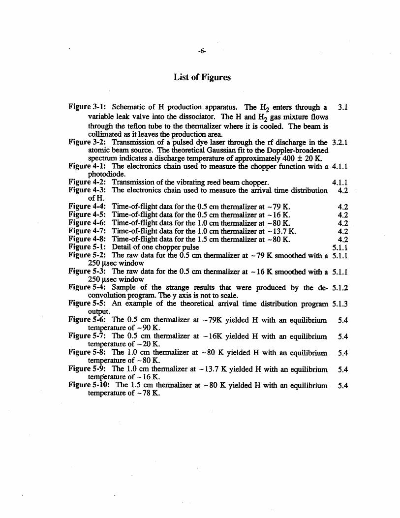
Figure 3-1: Schematic of H production apparatus. The H2 enters through a 3.1variable leak valve into the dissociator. The H and H2 gas mixture flowsthrough the teflon tube to the thermalizer where it is cooled. The beam iscollimated as it leaves the production area.

Figure 3-2: Transmission of a pulsed dye laser through the rf discharge in the 3.2.1atomic beam source. The theoretical Gaussian fit to the Doppler-broadenedspectrum indicates a discharge temperature of approximately 400 ± 20 K.

Figure 4-1: The electronics chain used to measure the chopper function with a 4.1.1photodiode.

Figure 4-2: Transmission of the vibrating reed beam chopper. 4.1.1Figure 4-3: The electronics chain used to measure the arrival time distribution 4.2

of H.Figure 4-4: Time-of-flight data for the 0.5 cm thermalizer at - 79 K. 4.2Figure 4-5: Time-of-flight data for the 0.5 cm thermalizer at - 16 K. 4.2Figure 4-6: Time-of-flight data for the 1.0 cm thermalizer at -80 K. 4.2Figure 4-7: Time-of-flight data for the 1.0 cm thermalizer at - 13.7 K. 4.2Figure 4-8: Time-of-flight data for the 1.5 cm thermalizer at -80 K. 4.2Figure 5-1: Detail of one chopper pulse 5.1.1Figure 5-2: The raw data for the 0.5 cm thermalizer at -79 K smoothed with a 5.1.1

250 ptsec windowFigure 5-3: The raw data for the 0.5 cm thermalizer at - 16 K smoothed with a 5.1.1

250 psec windowFigure 5-4: Sample of the strange results that were produced by the de- 5.1.2

convolution program. The y axis is not to scale.Figure 5-5: An example of the theoretical arrival time distribution program 5.1.3

output.Figure 5-6: The 0.5 cm thermalizer at -79K yielded H with an equilibrium 5.4

temperature of - 90 K.Figure 5-7: The 0.5 cm thermalizer at -16K yielded H with an equilibrium 5.4

temperature of - 20 K.Figure 5-8: The 1.0 cm thermalizer at -80 K yielded H with an equilibrium 5.4

temperature of - 80 K.Figure 5-9: The 1.0 cm thermalizer at - 13.7 K yielded IH with an equilibrium 5.4

temperature of - 16 K.Figure 5-10: The 1.5 cm thermalizer at -80 K yielded H with an equilibrium 5.4

temperature of - 78 K.

-7-

List of Tables

Table 3-I: Summary of H gas characteristics for thermalizers of different 3.4.2lengths.

Table 4-1: Summary of the parameters for each experimental run. 4.2Table 5-I: Relative H flux D is calculated for each experimental run. 5.2Table 5-II: H, signals and atomic dissociation percentage oz• for each 5.3

experimental run.Table 6-I: Summary of the measured quantities for each thermalizer length.

Chapter 1

Introduction

1.1 Background

Over the past forty-five years, atomic hydrogen beam sources have been used in a

variety of experiments. [1] [2] [3] [4] While room temperature atomic hydrogen beam

sources are commonplace, the development of cold sources is fairly recent. [5] With a cold

beam, the density is increased and the interaction time is lengthened. The apparatus

discussed in this thesis is used in an ongoing experiment whose goal is to measure the

Rydberg constant by high-precision millimeter-wave spectroscopy. [6] The experiment

uses the Ramsey separated oscillating field method, with a flight distance of 40 cm. For

this purpose, a beam with a temperature of - 15K is needed. A room temperature beam

would require a flight path of almost 2 m, which would be awkward. This experiment has

been built over the last three years and the author has been involved in its construction since

September, 1987 under the auspices of the Undergraduate Research Opportunities Program

at MIT.

1.2 Organization of Thesis

The thesis is organized as follows: In Chapter 2, the theory of beam formation,

including the derivation of the beam velocity distribution, will be presented. The

dissociation of H2 in a RF discharge and subsequent cooling of H by wall collisions in a

cold thermalized channel will be described in Chapter 3, and the detection of the beam will

be discussed in Chapter 4. In Chapter 5, the data from the beam measurements will be

analyzed as a function of the thermalizer length and temperature. The H flux, atomic

dissociation, and equilibrium beam temperature will also be calculated from the data for

-9-

each experimental configuration. Finally, an optimal thermalizer geometry will be

recommended on the basis of the above results.

-10-

Chapter 2

Theory Of Beam Formation

2.1 Flow Regimes

In kinetic theory, [7] an important parameter characterizing a gas is its mean free path

S- (2.1)2 an

where a is the collision cross section and n is the density of the gas. The mean free path is

the average distance that a particle traverses before interacting with a another particle. If

the gas is contained in a system with a characteristic dimension D, its kinetics may be

characterized by a Knudsen number Kn:

Kn = -. (2.2)D

Two flow regimes are of interest:

1. Kn < 0.01 continuum or viscous flow

2. Kn > 1.0 molecular or effusive flow

In continuum flow, the mean free path is small compared with the characteristic dimension

of the system. This implies that the flow will be determined primarily by gas-gas

interactions. In molecular flow, however, the mean free path is large and the flow

characteristics are determined by gas-wall interactions. In this case, the total flow rate 4

(atoms/second) across an orifice of cross-sectional area A is given by: [8]

nA <v>= 4 (2.3)

4

-11-

where <v> a (8 k T/i m) 2 is the average velocity of the particles. k is the Boltzmann

constant, and T is the gas temperature. The flux per solid angle for the orifice (atoms sec- l

sr-1) is given by

cose1(0) = .(2.4)

The flux in the forward direction is:

I(0) = *. (2.5)

For flow from a pipe, or some other elongated source, it is convenient to define X,the

directivity of the source, such that the forward flux per solid angle I is:

I = X . (2.6)

2.2 Molecular Gas Flow In Cylindrical Pipes

2.2.1 Definition of Flow Modes

A pipe is defined as a cylindrical object whose length L is long compared with its

characteristic dimension, the diameter D. Gas flow in pipes has been studied extensively by

Giordmaine and Wang. [9] In the molecular flow regime, there are two specific flow

modes which depend on the ratio of the mean free path to the pipe length:

1.Transparentmode: » >> LInthismode,X = 1

2. Opaque mode: X << Inthis mode,X < 1

In the transparent mode, the forward flux of the gas is given by Eq. (2.6) with X = 1:

nA <v>I = (2.7)4n

One may describe the flow through the pipe # by the Clausing formula: [10]t

-12-

KnA <v>4 = (2.8)

For a long cylindrical pipe, the Clausing factor K has the value 4 d / 3 L. The Clausing

factor is essentially the probability that a particle entering one end of a pipe will emerge

from the other end. The forward flux of the gas then becomes:

I - (2.9)xK

In the opaque mode, where X < < L / 2, the gas particles have a negligible chance

of passing through the pipe without collisions. The criterion for opacity is that

L / > 12. [9] Hence the flow conditions are totally different from the transparent mode

and the analysis is much more difficult. It can be shown that the directivity of the source is

given by: [5]

S= - [6 n <v> (2.10)8 D#

which, when substituted into Eq. (2.6), implies:

S[6 D n <v>A 1/2 (2.11)

The forward flux of the gas is independent of the pipe length, L, and is proportional to a2.

However, for a given flow rate, t, the forward flux is proportional to T'/4. Thist

demonstrates one of the inherent disadvantages of the opaque mode -- for a given flow rate,

as the temperature of gas is reduced, the forward flux is also reduced.

-13-

2.2.2 The Diffusion Model

In molecular flow, the flow rate of a gas in a long pipe is related to the gas density by

a one dimensional diffusion equation [5]:

4(z) = r ( r 2) dn(z) (2.12)3 dz

where r is the radius of the pipe and z is the distance from the high pressure end. Using this

result, we can estimate the average number of wall collisions that a gas particle makes

within a cylindrical pipe. This number is important in characterizing the thermalization

process described in Sec. 3.4.

Given a pipe of length L with boundary conditions 4(z = L) = 0 and 4(z = 0) = 9,,

Eq. (2.12) may be solved:

n(z) = no [-1 (2.13)

where

3 Lno 3 L +in (2.14)

2•n r 3 <v>

and r is the radius of the pipe.

The average number of wall collisions N, that a particle makes before emerging from

the pipe is given by the ratio of the flow rate to the walls of the pipe w., to the flow +t

from Eq. (2.8):

SwailNc (2.15)t

#waH may be found by evaluating the following integral:

-14-

IL1wal- = n(z) <v> 27cr dz. (2.16)

From Eq. (2.15), we obtain the following expression for the average number of wall

collisions:

3 2L 2N 3 - [2L] (2.17)

2.3 Measurement of the Velocity Distribution

A beam of gas particles in thermal equilibrium may be characterized by its

temperature. One can infer this temperature by using a bolometer which measures the

mean kinetic energy of the particles. A more elegant method is to measure the velocity

distribution of the gas and derive the gas temperature by comparing it to the theoretical

distribution function for an atomic beam in thermal equilibrium.

In thermal equilibrium, the velocity distribution of a gas is given by the Maxwell-

Boltzmann distribution:

f(v) dv = Vexp -v 1 dv (2.18)

with

a - (2kT/m)t/ 2 (2.19)

where m is the mass of the gas particle. a is known as the most probable velocity.

If the gas is sampled from an effusive beam, the distribution at the detector will be

velocity-weighted because the probability of a particle leaving the source is proportional to

its velocity: [11]

-15-

3v1

fb(v) dv = 2 exp -2 va2 dv (2.20)

To measure fb(v, we chop the beam and use time-of-flight (TOF) analysis. The arrival time

t for a group of particles with velocity v that leave the chopper at t is t - t = L/v where L0 0

is the chopper to detector distance. If s(t - t ) is the number of particles per area per time0

in the time interval (t, t+dt), then, since t = L/v, we have:

A dv(t ) = -f(v) - (2.21)0 b dt

If t =0,0

(t) = f (Lt) (L/t). (2.22)b

Our detector measures density and thus its efficiency has a v'- dependence. Consequently,

the signal from the detector, s(t) is related to s(t) by:

(t) (t) t f(L /t)s(t) = (t) = (2.23)

L t

Using Eq. (2.18), s(t), the number of particles per volume, then becomes:

s(t) = f (Lt) (L/t). (2.24)

or, equivalently,

s(t) = 4 t3 4exp[-L2/at (2.25)

Eq. (2.25) represents the number of particles seen at a detector a distance L from a

beam source at an equilibrium temperature T. In practice, the beam is chopped in order to

sample the distribution. If the duration of the chopper pulse is finite, the measured

distribution, 7(t) will be the convolution of the chopper function, r(t) with s(t):

-16-

7(t) f r(t) s(t - ) dt r(t) * s(t) (2.26)

Equivalently, from the convolution theorem,

T(f) = R(f) S(f) (2.27)

where Y(f), R(f), and S(f) are the Fourier transforms of the respective time distributions. In

the limit of a delta-function chopper,

S(t) = s(t) 4 Lt exp (2.28)

In our experiment, we determine the characteristics of the gas source by measuring the

arrival time distribution, s(t).

-17-

Chapter 3

Production of Atomic Hydrogen

3.1 Overview of Apparatus

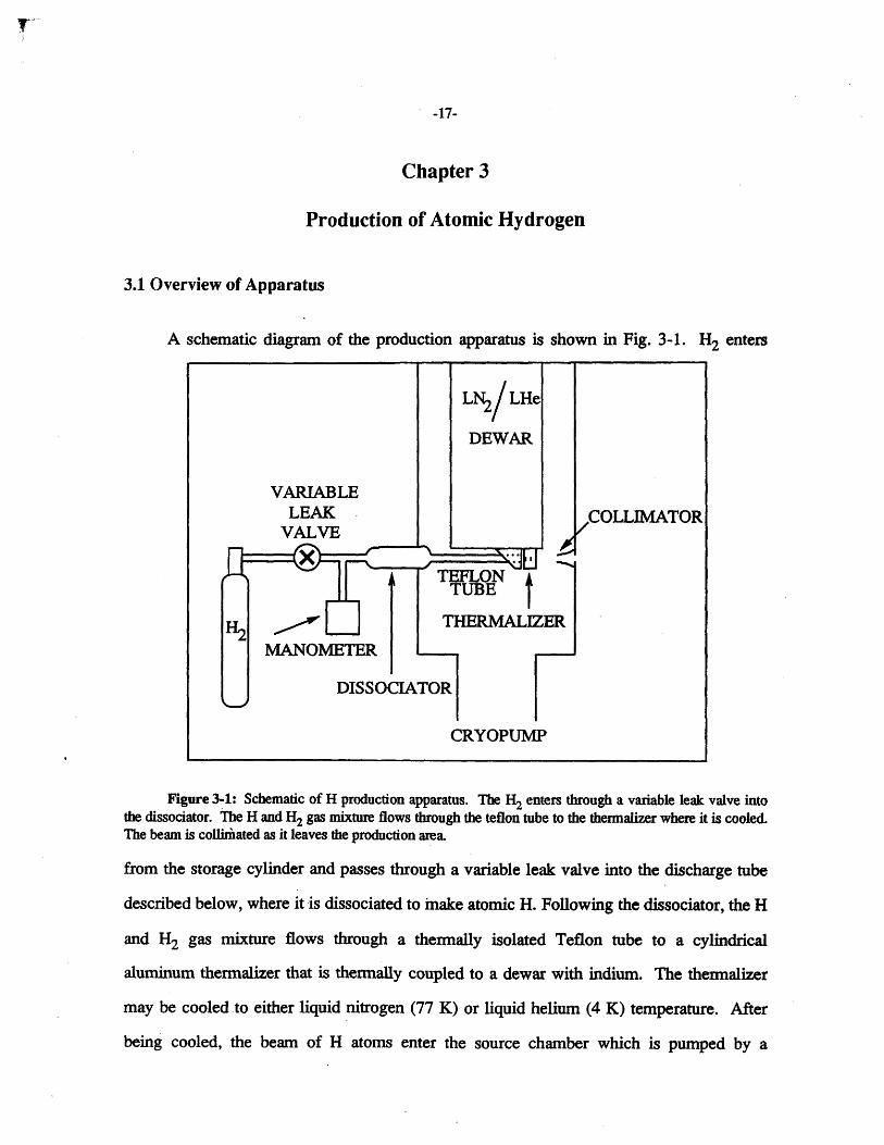
A schematic diagram of the production apparatus is shown in Fig. 3-1. H2 enters

Figure 3-1: Schematic of H production apparatus. The H2 enters through a variable leak valve intothe dissociator. The H and H2 gas mixture flows through the teflon tube to the thermalizer where it is cooled.The beam is colliziiated as it leaves the production area.

from the storage cylinder and passes through a variable leak valve into the discharge tube

described below, where it is dissociated to make atomic H. Following the dissociator, the H

and H2 gas mixture flows through a thermally isolated Teflon tube to a cylindrical

aluminum thermalizer that is thermally coupled to a dewar with indium. The thermalizer

may be cooled to either liquid nitrogen (77 K) or liquid helium (4 K) temperature. After

being cooled, the beam of H atoms enter the source chamber which is pumped by a

-18-

cryopump to a background pressure of 10-5 tonr. The three main parts of the production

apparatus will be discussed below.

3.2 Discharge Tube

The electrodeless discharge tube is based on a design by Slevin and Sterling [12].

The advantage of a RF discharge over a D.C. discharge is that there are no exposed

electrodes which can be sources of surface contamination. A self-sustaining RF discharge

is produced within a helical resonator operating at -80 MHz with -8 W power input.

Within the RF discharge, H2 molecules are dissociated by collisions with free electrons.

When enough random collisions have occurred, a chain reaction is established and the

ionization reaction reaches steady-state. The cavity has a Q of approximately 75 and was

originally designed for an input frequency of 100 MHz. Mechanical tolerance and

capacitative effects reduced the resonant frequency to approximately 80 MHz. The

dissociation fraction of hydrogen, defined as [H1]/([IHII]+[H 2]), was measured directly from

the discharge with a residual gas analyzer (cf. Sec. 4.1.2) and found to be approximately

80%.

3.2.1 Measurement of Discharge Temperature

To measure the temperature of the discharge, the Doppler width of the hydrogen gas

absorption spectrum was measured. For a spectral line of intensity To and frequency (o., the

intensity follows a Gaussian profile:

T() = To expL[ CO- (3.1)o) a

where c is the speed of light and a is the most probable velocity from Eq. (2.19). Since

a=(2 k T / m2), it is possible to deduce the gas temperature by measuring the Doppler-

-19-

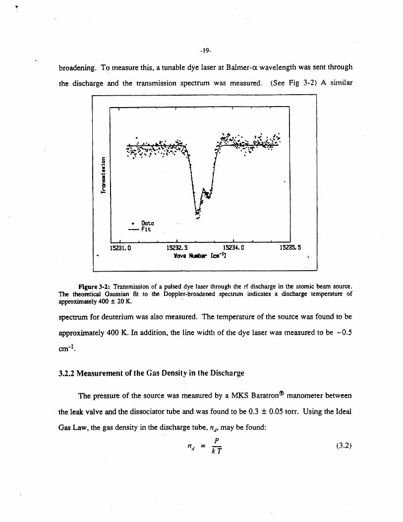
broadening. To measure this, a tunable dye laser at Balmer-cz wavelength was sent through

the discharge and the transmission spectrum was measured. (See Fig 3-2) A similar

Figure 3-2: Transmission of a pulsed dye laser through the rf discharge in the atomic beam source.The theoretical Gaussian fit to the Doppler-broadened spectrum indicates a discharge temperature ofapproximately 400 ± 20 K.

spectrum for deuterium was also measured. The temperature of the source was found to be

approximately 400 K. In addition, the line width of the dye laser was measured to be -0.5

cm-1 .

3.2.2 Measurement of the (Gas Density in the Discharge

The pressure of the source was measured by a MKS Baratron® manometer between

the leak valve and the dissociator tube and was found to be 0.3 ± 0.05 torr. Using the Ideal

Gas Law, the gas density in the discharge tube, nd, may be found:

n = -, (3.2)

C001

15231.0 15232. 5 15234. 15235.5Wave Number cmaJ]

SDato- Fit

I

I n

s l

e

-20-

where P is the gas pressure, and T = 400±20K is the discharge temperature. In this case,

nd = 7.2 ± 1.7 X 1015 cm 3.

3.3 Transport Tube

The design of the tube that transports atoms from the dissociator to the thermalizer is

critical. Its walls must have a low surface recombination constant and the gas density

within it must be low enough for volume recombination to be negligible. Teflon was used

because of its low surface recombination properties. The tubes that were utilized were 6.35

mm in diameter and -13 cm long. Near the thermalizer, the tube was connected to the

dewar by a Teflon support sleeve which thermally isolated the tube. At the end of this

sleeve, a 0.2 mm diameter aperture permitted the gas to exit the Teflon tube.

3.3.1 Determination of Output Flow Rate

In the limit that the ratio of output aperture area of the transport tube to input aperture

area from the dissociator approaches zero, the gas density at end of the tube n. is

approximately equal to nd, the density in the dissociator. Using the Clausing formula, Eq.

(2.8), one may then calculate the flow rate, out, at the end of the transport tube. In this

case, the Teflon tube has a diameter d = 0.635 cm and a typical length L = 13 cm. The

resulting Clausing factor K = 4d/ 3L = 6.7 X 10-2. The average velocity <v> is

calculated for a temperature of 400K and the cross-sectional area A = n d2 / 4 where d =

0.2 mm, the diameter of the aperture. The resulting flow rate is o, = 1.1 ± 0.3 X 1018

atoms/second.

3.3.2 Determination of Recombination Limits

Efficient transport from source to thermalizer requires low loss due to recombination.

Three types of recombination may occur: volume (3-body), second-order surface (2-body),

and first-order surface (adsorption). Consequently, recombination may be written as: [5]

-21-

dL= - r2Kvn 3 _ 2rKs2n2 _ 2rKs, (3.3)dz

where K, is the volume recombination rate, Ks2 is the second-order surface recombination

rate, and Ks, is the first-order surface recombination rate. Recombination on Teflon has

been verified to be a first-order process for temperatures between 100 K and 500

K. [13] This first-order rate coefficient is

Ks y <v> (3.4)

where y is the recombination probability per wall collision. Volume recombination may be

ignored if

KsIn > d K n3 (3.5)4

which implies

[4 Kn << • .1/2 (3.6)

LdKI

Substituting Eq. (3.4) into Eq. (3.6) implies:

n [y <<>dK ] (3.7)V

For Teflon, the parameters y and K, have been measured [13] to be 2.1 X 10-5 and 1.2 X

10-32 cm6 atom-2 sec-1, respectively. Hence the requirement for neglecting volume

recombination is n< < 2.8 X 1016 cm-3 for teflon, which is satisfied in this case.

-22-

3.4 Thermalizer

Because a slow (10 - 80 K) H beam is needed, it must be cooled from the discharge

temperature of approximately 400 K. This is done by passing the beam through a

thermalizer which is kept at the desired temperature. Various thermalizer designs using

pyrex and copper have been described in the literature. [4] [14] Aluminum was chosen

because of its performance in a similar apparatus. [5] Surface recombination is expected to

occur rapidly on an aluminum surface, but it is believed that the A120 3 surface, which is

always present on Al exposed to air, has a low recombination coefficient. The thermalizer

is thermally coupled to a LN2/LHe dewar with strips compressed strips of indium. A

silicon diode thermometer is attached to the side of the thermalizer to monitor its

temperature. It was discovered (cf. Sec 5.4) that temperature gradients due to the thermal

load from recombination cause discrepancies between the temperature of the beam and the

measured temperature of the thermalizer.

3.4.1 Description of Thermalizers Studied

To examine the effect of the thermalizer length on the thermalization of the H atoms,

three aluminum thermalizers of lengths 0.5 cm., 1.0 cm., and 1.5 cm. with 0.2 cm diameter

holes were constructed. For this purpose, the existing copper "can" which couples the

thermalizer to the dewar was modified to accept thermalizers of different lengths. A Teflon

support sleeve was constructed for each thermalizer

3.4.2 Determination of Flow Regime and Average Number of Wall Collisions

Although there is a small (0.5 mm) gap between the Teflon sleeve and the aluminum

thermalizer, this gap has a relatively high flow impedance compared to the thermalizer

channel and hence the flow rate into the thermalizer therm,, is approximately equal to the

value of o,,, calculated in Sec. 3.3.1. If the downstream end of the thermalizer is in high

-23-

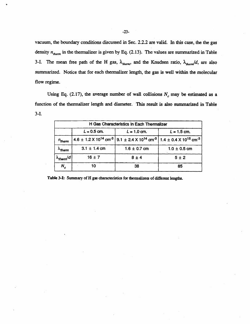
vacuum, the boundary conditions discussed in Sec. 2.2.2 are valid. In this case, the the gas

density nt,,he in the thermalizer is given by Eq. (2.13). The values are summarized in Table

3-I. The mean free path of the H gas, th,,n, and the Knudsen ratio, Xther/d, are also

summarized. Notice that for each thermalizer length, the gas is well within the molecular

flow regime.

Using Eq. (2.17), the average number of wall collisions Nc may be estimated as a

function of the thermalizer length and diameter. This result is also summarized in Table

3-I.

H Gas Characteristics In Each Thermalizer

L = 0.5 cm. L = 1.0 cm. L = 1.5 cm.

ntherm 4.6 ± 1.2 X 1014 cm "3 9.1 ± 2.4 X 1014 cm-3 1.4 ± 0.4 X 101s cm "3

'therm 3.1 ± 1.4 cm 1.6 ± 0.7 cm 1.0 + 0.5 cm

,thern/d 16 ± 7 8 ± 4 5 ± 2

Nc 10 38 85

Table 3-I: Summary of H gas characteristics for thermalizers of different lengths.

-24-

Chapter 4

Detection of Atomic Hydrogen

4.1 Overview of Detection Apparatus

After leaving the thermalizer in the source chamber, the H beam passes through a

collimator which defines the beam's shape. It then passes through a chopper in front of a

slit which can let a short pulse of the beam enter the main chamber. After progressing

135.6 cm down the length of the chamber, the beam is detected by a residual gas analyzer.

The data presented in this thesis were analyzed with a lock-in amplifier and time-of-flight

data was obtained by a CAMAC-based data acquisition system and a Tandon AT

Computer.

4.1.1 Chopper

The vibrating reed chopper was based on a design by P5hlmann, et al. [15]. A thin

aluminum reed forms one plate of a parallel plate capacitor. An oscillating high voltage on

the other plate drives the reed at its resonant frequency of 110 Hz. The chopper opens

twice every cycle which results in a beam chopping frequency of 220 Hz.

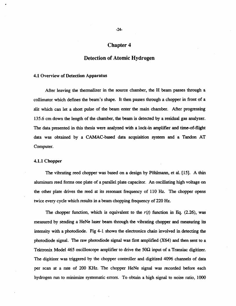
The chopper function, which is equivalent to the r(t) function in Eq. (2.26), was

measured by sending a HeNe laser beam through the vibrating chopper and measuring its

intensity with a photodiode. Fig 4-1 shows the electronics chain involved in detecting the

photodiode signal. The raw photodiode signal was first amplified (X64) and then sent to a

Tektronix Model 465 oscilloscope amplifier to drive the 50C input of a Transiac digitizer.

The digitizer was triggered by the chopper controller and digitized 4096 channels of data

per scan at a rate of 200 KHz. The chopper HeNe signal was recorded before each

hydrogen run to minimize systematic errors. To obtain a high signal to noise ratio, 1000

-25-

Figure 4-1: The electronics chain used to measure the chopper function with a photodiode.

scans of the chopper signal were summed. An additional 1000 scans were taken with the

HeNe laser blocked to record any noise associated with the measurement chain. This data

was subtracted from the chopper signal to produce the chopper function for each individual

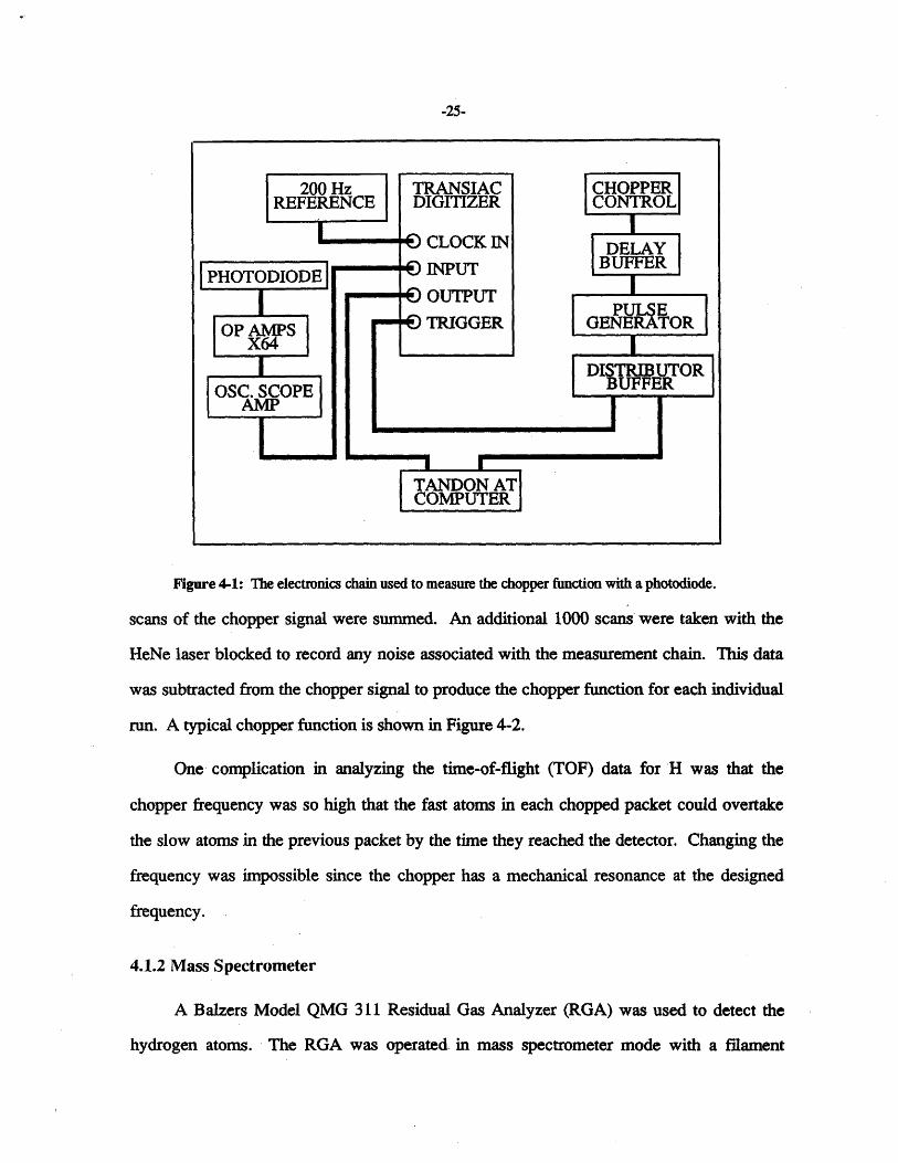
run. A typical chopper function is shown in Figure 4-2.

One complication in analyzing the time-of-flight (TOF) data for H was that the

chopper frequency was so high that the fast atoms in each chopped packet could overtake

the slow atoms in the previous packet by the time they reached the detector. Changing the

frequency was impossible since the chopper has a mechanical resonance at the designed

frequency.

4.1.2 Mass Spectrometer

A Balzers Model QMG 311 Residual Gas Analyzer (RGA) was used to detect the

hydrogen atoms. The RGA was operated in mass spectrometer mode with a filament

-26-.. .... .................. ... ..... ... .............. ................ .... ....

1.0

~0.8

S0.6

-- 0.4aU0J

Time [mill1seconds]

Figure 4-2: Transmission of the vibrating reed beam chopper.

emission current of 1 mA. and a Secondary Electron Multiplier (SEM) bias of 2750 V. In

this mode, atoms are detected if they fall within a certain mass range. Hence, it is possible

to set the RGA to detect particles of atomic mass 1 (H) or atomic mass 2 (H2).

4.2 Measurement of Hydrogen Distribution

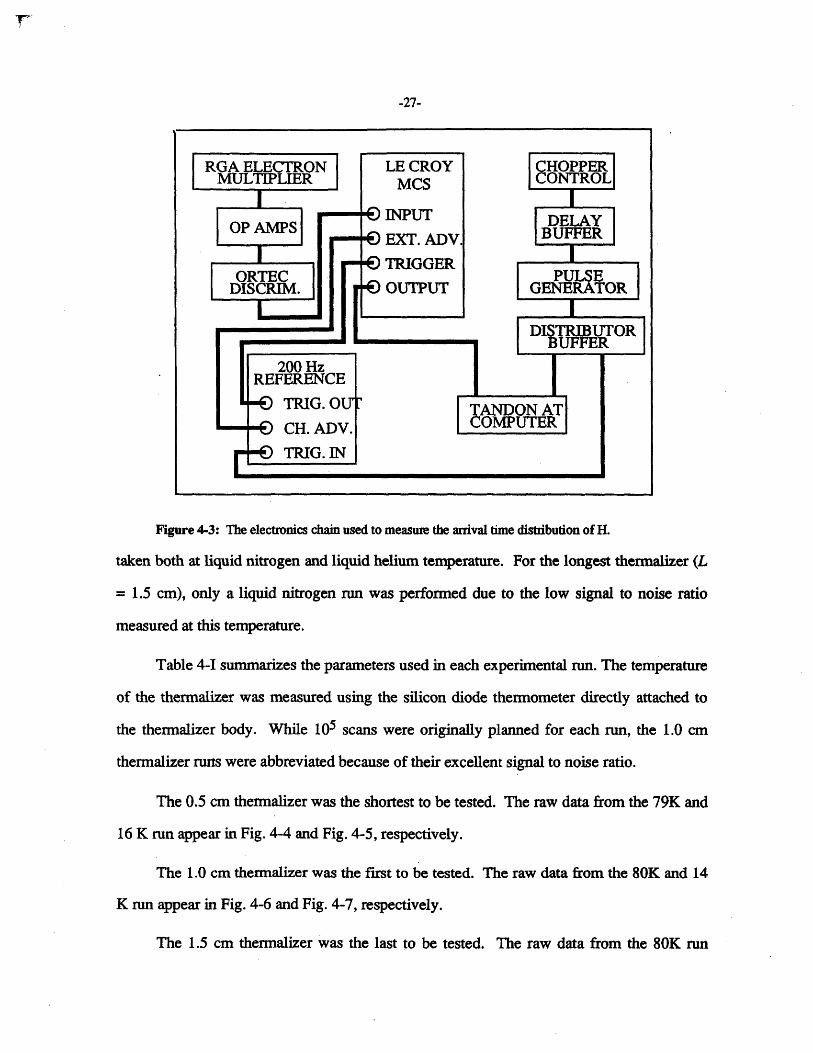
The electron multiplier signal from the RGA is processed by the electronics chain as

shown in Fig. 4-3. The 200 Hz reference clock provides the time base which is gated by the

chopper control. After passing through several amplifiers, the pulses from the SEM are

analyzed by an ORTEC Model 473 discriminator. The output signal from the ORTEC

discriminator was then fed into a LeCroy Model 3521A multi-channel scaler (MCS). This

device digitized 4096 channels per data scan at 200 KHz. To obtain a high signal to noise

ratio, 105 scans were taken per run which resulted in each run lasting approximately 3

hours. For two of the three thermalizers (L = 0.5 cm and 1.0 cm), the TOF spectra were

II I I · I

ij Qi 1J Lj~

-27-

Figure 4-3: The electronics chain used to measure the arrival time distribution of H.

taken both at liquid nitrogen and liquid helium temperature. For the longest thermalizer (L

= 1.5 cm), only a liquid nitrogen run was performed due to the low signal to noise ratio

measured at this temperature.

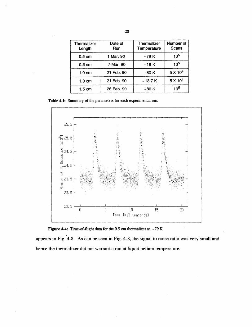
Table 4-I summarizes the parameters used in each experimental run. The temperature

of the thermalizer was measured using the silicon diode thermometer directly attached to

the thermalizer body. While 105 scans were originally planned for each run, the 1.0 cm

thermalizer runs were abbreviated because of their excellent signal to noise ratio.

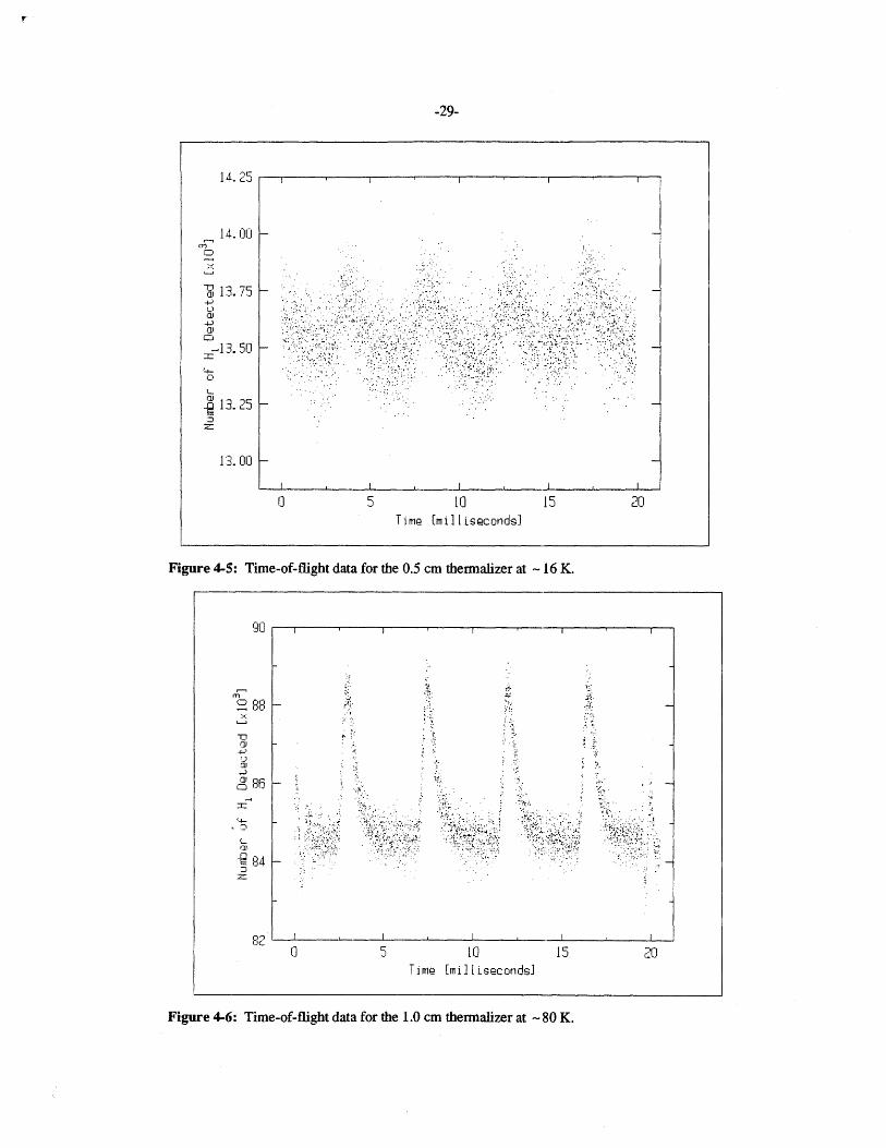
The 0.5 cm thermalizer was the shortest to be tested. The raw data from the 79K and

16 K run appear in Fig. 4-4 and Fig. 4-5, respectively.

The 1.0 cm thermalizer was the first to be tested. The raw data from the 80K and 14

K run appear in Fig. 4-6 and Fig. 4-7, respectively.

The 1.5 cm thermalizer was the last to be tested. The raw data from the 80K run

-28-

Thermalizer Date of Thermalizer Number ofLength Run Temperature Scans

0.5 cm 1 Mar. 90 -79 K 105

0.5 cm 7 Mar. 90 -16 K 10s

1.0 cm 21 Feb. 90 -80 K 5 X 104

1.0 cm 21 Feb. 90 -13.7 K 5 X 104

1.5 cm 26 Feb. 90 -80 K 105

Table 4-I: Summary of the parameters for each experimental run.

Figure 4-4: Time-of-flight data for the 0.5 cm thermalizer at -79 K.

appears in Fig. 4-8. As can be seen in Fig. 4-8, the signal to noise ratio was very small and

hence the thermalizer did not warrant a run at liquid helium temperature.

F- -- I I I

25.5

_ 25. O0

- 24. 5

4,o

~24.0

o

2~ 3. 5

??

0 5 t0 15 20Time [mi11Lseconds]

I·:: .111·· '2.'.'

\·,··:· ·''''i. .··r; i

t .l

··· i· ·:· r.

v ~· ~, · :i

i r; i:::~

:· : 4:1~. pc:.: ~r·-··..1:;·:I.I~.. :·):··:· · ·:·.

i ··:·-i; !~ :· ·r'' ···.'.:·)'; .:m r-:c·

··,·; ·:;~:· ··.:..: ~--. ·. ..-r· · ·· :-~"'"'`i· ~··:.~i:'' · · ·..ii,··'' .. ;..,., 1 ;·(··'·-· ·;: ~i~~~il··;"·· -·.~-···...

·̀·

I , I I , I , I

-29-

Figure 4-5: Time-of-flight data for the 0.5 cm thermalizer at - 16 K.

Figure 4-6: Time-of-flight data for the 1.0 cm thermalizer at - 80 K.

14. Ld

14. 00

- 13.7503

cuoJ4-)

03.5014-

S13.25

13. 00

0 5 10 15 20Time [millLseconds]

I , , -~ i ,- i

i

..··- :.····-~.:::j· ,i··.: ; .·, ;:·

c ·:·~·· · · · :· :? ·:i ;:·..··~ ~~:·· ::··;..i~ ··:~ .... ~··

····.r;" ·::· :,"' ': ""' `·· .2· ··::· ·,.,··· ·;·· -1· ·:.;':::. ·"·:.·

.'.. ·· I··~.::. ... ;. .;. .·.iC. .~.. i ··::h: ·,-:;~r:i·~~.~,:.· :'''·· · ~.L :;,,;

'' I· 'A·, '· ·"r·. : ·.r?·.:·r·· .v r'.··~ .... ~

.r~'··~'~ ~:··-L' i.: 'L·''· ·· · '' :· :· '" .I~·~'· ·.'" '' ·:~s?~. ·· ····;;.:·· ·

rI , I , I , r , I

i I I I

;..•; ::•

.- ,'. '...- . . .

..

I , I I I f I

2 8x

cu

ID

L-rU

984

Q _

0 5 10 15 20Time [millseconds]

ii CIT

nn

Ir· e: '~ -i

'"~ij ;; -r ·· i :'"B r

·1 i ; · ·i~ ·;·

~· '· :?·

'r 'f:: ~~

··.~~· · ~···r r·,r·.. fh· i

"'(* i''~.~· ·. ·; ..

·:i ··· t.~·1·: ~-~r .~C- .

-30-

Figure 4-7: Time-of-flight data for the 1.0 cm thermalizer at - 13.7 K.

Figure 4-8: Time-of-flight data for the 1.5 cm thermalizer at - 80 K.

S I I I 1 I I

S84

O

823

Time (milliseconds]

I

· · · ·

I , I I ,

Time [mi]IL•cond•]

............ ... .......... .. .. ..... .. .... ............. ................................. .......... ........ .. ....... .......... ................. .................

I I , I

..... ........ ........ -----

-31-

Chapter 5

Analysis of Data

5.1 Data Reduction Programs

The analysis of the time-of-flight (TOF) data was done on an IBM RT Personal

Computer. All of the computer code was written in the C language. Some of the code was

based on programs discussed in Numerical Recipies in C. [16]

5.1.1 Smoothing

As can be seen in Figures 4-4 through 4-8, the data was very noisy. The smoothing

program in Appendix A was used to smooth the data. A user defined window is input along

with the data to be smoothed. The Fourier transform of the data is calculated and passed

through a filter whose size is proportional to the window. By varying the width of the

window, various degrees of smoothing can be obtained. To determine the width of the

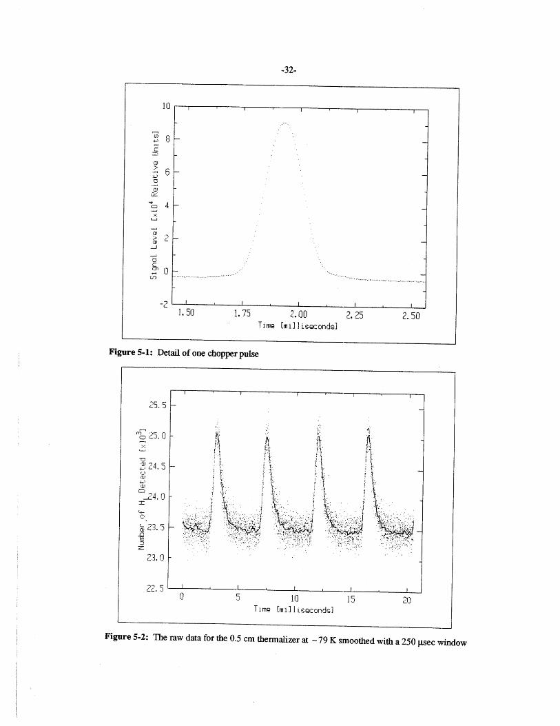
window, the width of the chopper pulse was examined in detail. The first chopper pulse

from Fig. 4-2 is shown in Fig. 5-1.

The total width of the peak was estimated from Fig. 5-1 to be 650 Rsec. This

corresponds to 130 channels from the original 4096 channels of data so that the signal is

extremely well' resolved. The full width at half-maximum was measured to be 190 I±sec

which is equivalent to 38 data channels. The output of the smoothing program was

examined for various window widths and a width of 250 Csec (50 channels) was chosen to

smooth the data. This was to eliminate as much noise as possible while guaranteeing that

no important information in the raw data was washed out. Examples of this smoothing are

shown in Fig. 5-2 and Fig 5-3.

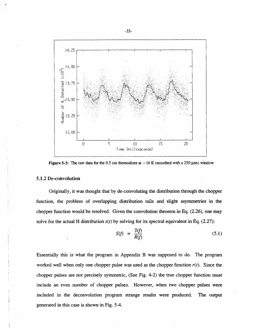
Fig. 5-3 clearly shows the chopper-frequency problem described in Sec. 4.1.1. The

tail of each velocity distribution runs into the subsequent ones.

-32-

SJ

6

SI I

......... ...............I.......... ... . . . . ...

.......75. ...... I5 ..........................Time [mi···ecnd£

1.50 1.75 2.00 2.25 2.50Time [milliseconds]

Figure 5-1: Detail of one chopper pulse

25. 5

1 25. O

C)

234. 5

23. 01

22. 50 5 10 15 20

Time [millis•c•nrlnd

Figure 5-2: The raw data for the 0.5 cm thermalizer at -79 K smoothed with a 250 psec window

,,i I I

I

II

-L: I I I

r

Figure 5-1:

Detail of one chopper

pulse

-----------F-

I

-33-

Figure 5-;3: The raw data for the 0.5 cm thermalizer at - 16 K smoothed with a 250 plsec window

5.1.2 De-convolution

Originally, it was thought that by de-convoluting the distribution through the chopper

function, the problem of overlapping distribution tails and slight asymmetries in the

chopper function would be resolved. Given the convolution theorem in Eq. (2.26), one may

solve for the actual H distribution s(t) by solving for its spectral equivalent in Eq. (2.27):

(f) - (5.1)R(f)

Essentially this is what the program in Appendix B was supposed to do. The program

worked well when only one chopper pulse was used as the chopper function r(t). Since the

chopper pulses are not precisely symmetric, (See Fig. 4-2) the true chopper function must

include an even number of chopper pulses. However, when two chopper pulses were

included in the deconvolution program strange results were produced. The output

generated in this case is shown in Fig. 5-4.

I r I I I -- 1 --1 A ?C14. .3

14. 00

Y 13.75o

a:-,

-,13.50-r"

014.-o

L

13.25

13.00

0 5 10 15Time [milliseconds]

·. · ~

I , I , I I I

-34-

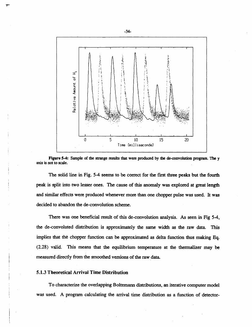
Figure 5-4: Sample of the strange results that were produced by the de-convolution program. The yaxis is not to scale.

The solid line in Fig. 5-4 seems to be correct for the first three peaks but the fourth

peak is split into two lesser ones. The cause of this anomaly was explored at great length

and similar effects were produced whenever more than one chopper pulse was used. It was

decided to abandon the de-convolution scheme.

There was one beneficial result of this de-convolution analysis. As seen in Fig 5-4,

the de-convoluted distribution is approximately the same width as the raw data. This

implies that the chopper function can be approximated as delta function thus making Eq.

(2.28) valid. This means that the equilibrium temperature at the thermalizer may be

measured directly from the smoothed versions of the raw data.

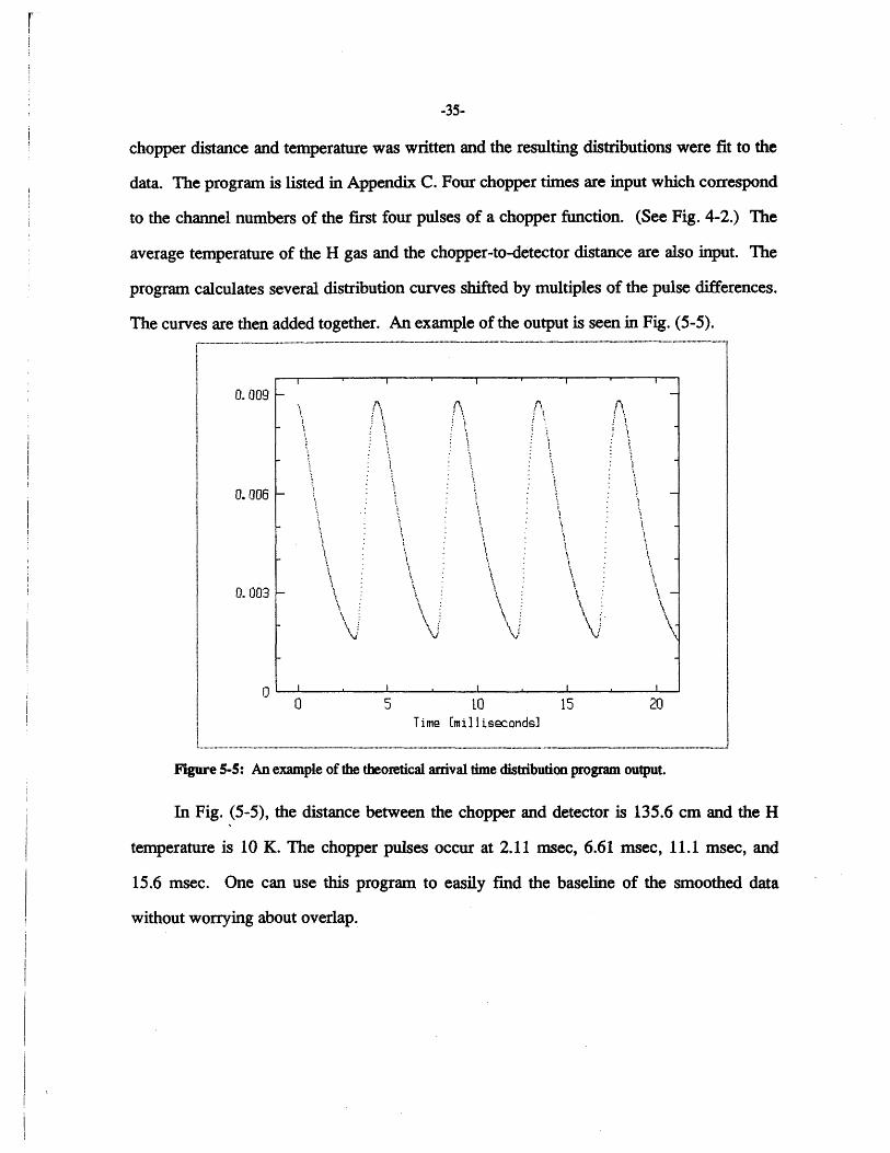
5.1.3 Theoretical Arrival Time Distribution

To characterize the overlapping Boltzmann distributions, an iterative computer model

was used. A program calculating the arrival time distribution as a function of detector-

I I I I I

- I I I I

04I(3

0

ai0::

0 5 [o 15 20Time [milliseconds]

-35-

chopper distance and temperature was written and the resulting distributions were fit to the

data. The program is listed in Appendix C. Four chopper times are input which correspond

to the channel numbers of the first four pulses of a chopper function. (See Fig. 4-2.) The

average temperature of the H gas and the chopper-to-detector distance are also input. The

program calculates several distribution curves shifted by multiples of the pulse differences.

The curves are then added together. An example of the output is seen in Fig. (5-5).

Figure 5-5: An example of the theoretical arrival time distribution program output.

In Fig. (5-5), the distance between the chopper and detector is 135.6 cm and the H

temperature is 10 K. The chopper pulses occur at 2.11 msec, 6.61 msec, 11.1 msec, and

15.6 msec. One can use this program to easily find the baseline of the smoothed data

without worrying about overlap.

I I I ' I I I

, : .•

i • •

•~ i\ ?i ?

i • ' •,,

I , I , I

0. 009

0. 006

0. 003

n

0 5 tO 15 20Time (militseconds]

........ ....... ............ ................... .... .......... .... ... ............ .... .............. ...

\

-36-

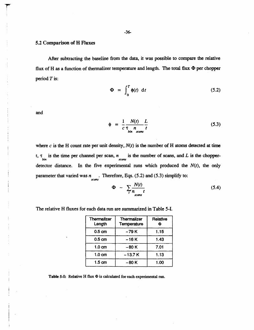
5.2 Comparison of H Fluxes

After subtracting the baseline from the data, it was possible to compare the relative

flux of H as a function of thermalizer temperature and length. The total flux ( per chopper

period T is: rT0 = 0(t) dt (5.2)

and

1 N(t) L (5.3)c' n tbin scans

where c is the H count rate per unit density, N(t) is the number of H atoms detected at time

t, t is the time per channel per scan, n is the number of scans, and L is the chopper-bin scans

detector distance. In the five experimental runs which produced the N(t), the only

parameter that varied was n . Therefore, Eqs. (5.2) and (5.3) simplify to:scans

S N(t) (5.4)n t

scans

The relative H fluxes for each data run are summarized in Table 5-I.

Thermalizer Thermalizer RelativeLength Temperature 0

0.5 cm -79 K 1.15

0.5 cm -16 K 1.43

1.0 cm -80 K 7.01

1.0 cm -13.7 K 1.13

1.5 cm -80 K 1.00

Table 5-I: Relative H flux a( is calculated for each experimental run.

-37-

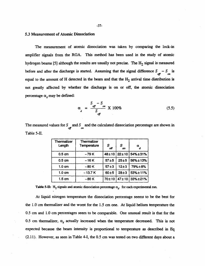
5.3 Measurement of Atomic Dissociation

The measurement of atomic dissociation was taken by comparing the lock-in

amplifier signals from the RGA. This method has been used in the study of atomic

hydrogen beams [5] although the results are usually not precise. The H2 signal is measured

before and after the discharge is started. Assuming that the signal difference S - S isoff on

equal to the amount of H detected in the beam and that the H2 arrival time distribution is

not greatly affected by whether the discharge is on or off, the atomic dissociation

percentage ad may be defined:

S -Sa = of on X 100% (5.5)

d Soff

The measured values for S and S and the calculated dissociation percentage are shown inoff on

Table 5-II.

Thermalizer ThermalizerLength Temperature S S a

off on d

0.5 cm -79 K 48±10 22±10 54%±31%0.5 cm -16 K 57±5 25±5 56%±13%

1.0 cm -80 K 57±3 12±3 79%± 8%

1.0 cm -13.7 K 60±5 28±3 53%±11%

1.5 cm -80 K 70±10 47±10 33%±21%

Table 5-II: Hz signals and atomic dissociation percentage ad for each experimental run.

At liquid nitrogen temperature the dissociation percentage seems to be the best for

the 1.0 cm thermalizer and the worst for the 1.5 cm one. At liquid helium temperature the

0.5 cm and 1.0 cm percentages seem to be comparable. One unusual result is that for the

0.5 cm thermalizer, ad actually increased when the temperature decreased. This is not

expected because the beam intensity is proportional to temperature as described in Eq

(2.11). However, as seen in Table 4-I, the 0.5 cm was tested on two different days about a

-38-

week apart. It is possible that some surface contamination in the Teflon tube or the

thermalizer was cleared up after several days under vacuum.

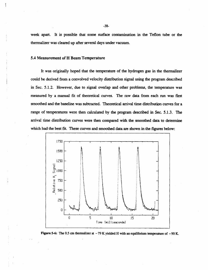
5.4 Measurement of H Beam Temperature

It was originally hoped that the temperature of the hydrogen gas in the thermalizer

could be derived from a convolved velocity distribution signal using the program described

in Sec. 5.1.2. However, due to signal overlap and other problems, the temperature was

measured by a manual fit of theoretical curves. The raw data from each run was first

smoothed and the baseline was subtracted. Theoretical arrival time distribution curves for a

range of temperatures were then calculated by the program described in Sec. 5.1.3. The

arrival time distribution curves were then compared with the smoothed data to determine

which had the best fit. These curves and smoothed data are shown in the figures below:

Figure 5-6: The 0.5 cm thermalizer at - 79 K yielded H with an equilibrium temperature of - 90 K.

1750

1500

1250

1 000-r-

• 750

500

250

0

0 5 10 15 20Time [milltsQconds]

-39-

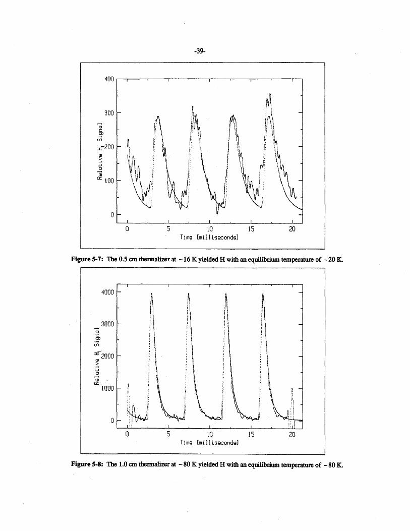
Figure 5-7: The 0.5 cm thermalizer at - 16 K yielded H with an equilibrium temperature of - 20 K.

Figure 5-8: The 1.0 cm thermalizer at - 80 K yielded H with an equilibrium temperature of - 80 K.

4UU

300

aJ

0

cr 100

0 5Time [milIiseconds]

I

II 1II 'I ii

I I I

4000

3000

U)

: 2000

C,

1000

0 5 10 15 20Time [millLseconds]

Inn

Tim• [mi]IL•ond•]

I I

-40-

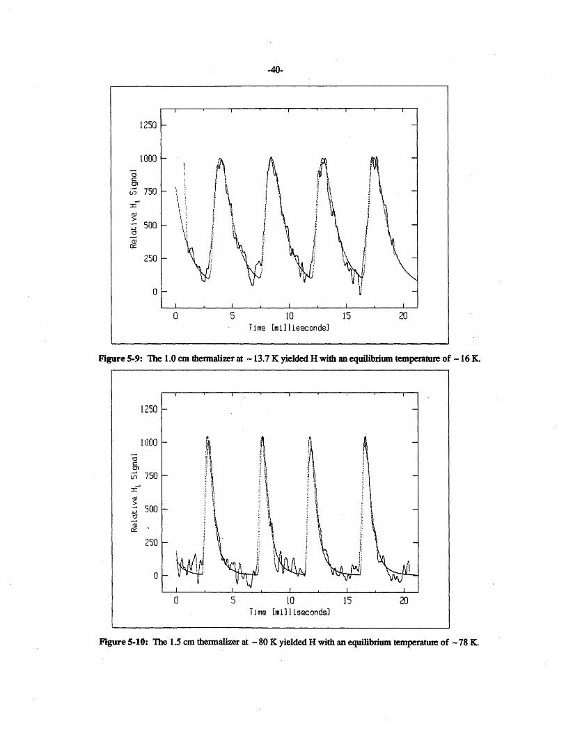
Figure 5-9: The. 1.0 cm thermalizer at - 13.7 K yielded H with an equilibrium temperature of - 16 K.

Figure 5-10: The 1.5 cm thermalizer at - 80 K yielded H with an equilibrium temperature of - 78 K.

1250

1000

b 750

500

250

0

Time [millisecondsl

1250

1100

WO

c 750-I-

500

250

0

Time [mi11Lseconds]

Time [mi] I Lseconds]

--

Time [mill Lseconds]

-41-

Chapter 6

Conclusion

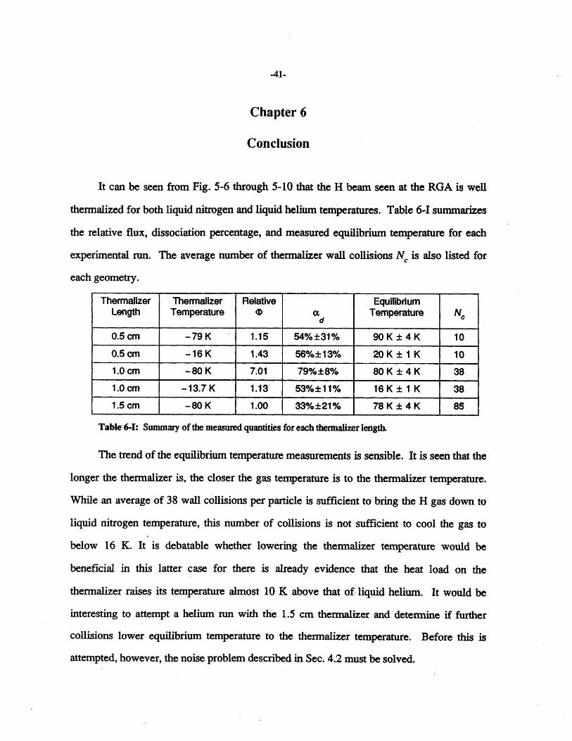
It can be seen from Fig. 5-6 through 5-10 that the H beam seen at the RGA is well

thermalized for both liquid nitrogen and liquid helium temperatures. Table 6-I summarizes

the relative flux, dissociation percentage, and measured equilibrium temperature for each

experimental run. The average number of thermalizer wall collisions Nc is also listed for

each geometry.

Thermalizer Thermalizer Relative EquilibriumLength Temperature 0 a Temperature Ncd

0.5 cm -79 K 1.15 54%±31% 90 K ± 4 K 10

0.5 cm -16 K 1.43 56%± ±13% 20 K ± 1 K 101.0 cm -80 K 7.01 79%±8% 80 K ± 4 K 381.0 cm -13.7 K 1.13 53%±11% 16 K ± 1 K 381.5 cm -80 K 1.00 33%±21% 78 K ± 4 K 85

Table 6-I: Summary of the measured quantities for each thermalizer length.

The trend of the equilibrium temperature measurements is sensible. It is seen that the

longer the thermalizer is, the closer the gas temperature is to the thermalizer temperature.

While an average of 38 wall collisions per particle is sufficient to bring the H gas down to

liquid nitrogen temperature, this number of collisions is not sufficient to cool the gas to

below 16 K. It is debatable whether lowering the thermalizer temperature would be

beneficial in this latter case for there is already evidence that the heat load on the

thermalizer raises its temperature almost 10 K above that of liquid helium. It would be

interesting to attempt a helium run with the 1.5 cm thermalizer and determine if further

collisions lower equilibrium temperature to the thermalizer temperature. Before this is

attempted, however, the noise problem described in Sec. 4.2 must be solved.

-42-

Another interesting result which depends on thermalizer length is the relative flow

rate 0. From arguments in Sec 2.2.1, it should be expected that the flow rate should be

proportional to the temperature of the source. The results from the 1.0 cm thermalizer are

in agreement with this theory while the 0.5 cm thermalizer exhibits an increase in flux when

run at liquid helium temperature. Since the two 0.5 cm measurements were taken about a

week apart, it is possible that the source was partially blocked by some foreign matter

during the 80 K run and, after continued vacuum pumping, this matter was removed.

Further experiments with the 0.5 cm thermalizer should be considered.

In light of the present results, it must be deduced that the optimal length of the

thermalizer in this apparatus is 1.0 cm. The relative flux is the greatest for this length and

the equilibrium temperature of the resulting beam is in excellent agreement with the

measured thermalizer temperature. However, as previous stated, this result should not be

taken as conclusive until a more thorough study of the shorter thermalizer is undertaken.

-43-

References

[1] S. B. Crampton, T. J. Greytak, D. Kleppner, W. D. Phillips, D. A. Smith, andA. Weinrib.Hyperfine Resonance of Gaseous Atomic Hydrogen at 4.2 K.Physical Review Letters , 42(1039), 1979.

[2] W. N. Hardy, A. J. Berlinsky, and L. A. Whitehead.Magnetic Resonance Studies of Gaseous Atomic Hydrogen at Low Temperature.Physical Review Letters , 42(1042), 1979.

[3] M. Morrow, R. Jochemsen, A. J. Berlinsky, and W. N. Hardy.Zero-Field Hyperfmine Resonance of Atomic Hydrogen for 0.18 K #•# T #-# 1 K:

The Binding Energy of H on Liquid 4He.Physical Review Letters , 46(195), 1981.

[4] J. P. Toennies, W. Welz, and G. Wolf.Molecular Beam Scattering Studies of Orbiting Resonances and the Determination

of van der Waals Potentials for H-Ne, Ar, Kr, and Xe and for H2-Ar, Kr, Xe.Journal of Chemical Physics , 71(614), 1979.

[5] J. T. M. Walraven and Isaac F. Silvera.Helium-Temperature Beam Source of Atomic Hydrogen.Review of Scientific Instruments , 53(8), 1982.

[6] Research Laboratory of Electronics.Annual Report #132.Technical Report, Massachusetts Institute of Technology,, 1989.

[7] O'Hanlon.A User's Guide to Vacuum Technology.John Wiley & Sons, 1989.

[8] D. Singy, P. A. Schmelzbach, W. Griiebler, W. Z. Zhang.Production of Intense Polarized Hydrogen Atomic Beams by Cooling the Atoms to

Low Temperature.Nuclear Instruments and Methods in Physics Research A: Accelerators,

Spectrometers, Detectors, and Associated Equipment, 278(349), 1988.

[9] J. A. Giordmaine and T. C. Wang.Molecular Beam Formation by Long Parallel Tubes.Journal of Applied Physics , 31(463), 1960.

[10] P. Clausing.Ober die Strahlformung bei der Molekularstr6mung.Zeitschrift fiir Physik , 66(471), 1930.

-44-

[11] N. F. Ramsey.Molecular Beams.Clarendon, Oxford, 1956.

[12] J. Slevin and W. Stirling.Radio Frequency Atomic Hydrogen Beam Source.Review of Scientific Instruments , 52(1780), 1981.

[13] D. N. Mitchell and D. J. Le Roy.An Experimental Test of Orbiting Resonance Theory of Hydrogen Atom

Recombination at Room Temperature.Journal of Chemical Physics , 67(1042), 1977.

[14] H. Wilsch.Remark on the Cooling of Atomic Hydrogen Beams.Journal of Chemical Physics , 56(1412), 1971.

[15] E. Pihlman, R. Hiittl, and H. Knecht.Self-maintained Reed Chopper for Beam Modulation in UHV.Journal of Physics E: Scientific Instruments, 20(455), 1987.

[16] W. H. Press, B. P. Flannery, S. A. Teukolsky, W. T. Vetterling.Numerical Recipies in C.Cambridge University Press, 1988.

-45-

Appendix A

The following is C code for the smoothing program described in Sec. 5.1.1:

Makefile

# This is the Makefile to make the data smoothing program.LIBS = -imCC = cc

main.o: main. ccc -a -c main.c

OBJ = main.o smooft.o realft.o fourl.o nrutil.o

smoot: $ (OBJ)$(CC) -a -i -o smoot $(LDFLAGS) $(OBJ) $(LIBS)

$ (OBJ) : malloc.h

malloc.h

#define voidchar *malloc();void free ();

main.c/*

This is the main.c for the data smoothing program.This program calls the following programs fromPress, et. al., _Numerical Recipies in C_, 1989:smooft.c, fourl.c, realft.c nrutil.c

*/

#include <math.h>#include <stdio. h>#define SIZE 4096#define ySIZE 32768#define float double#define CHECK 0

main(argc, argv)

-46-

int argc;char *argv [ ];

int i,j,jim,nu,n;long int dummy2, dummyl;static double y[SIZE +1],pts,double newdummyl[SIZE + 1];float smooft ();char *datafile, dataname[30],FILE *fp, *fopen();

presmooth[SIZE +1];

line[128];

datafile = dataname;if(argc != 3)

{fprintf(stderr, "Usage: smoot window datafile\n\n");exit (1);

else {pts = atof(argv[1]);datafile = argv[2];I

nu = n = SIZE;/*pts = 5.0;*/fprintf(stderr, "OK\n");

fp = fopen(datafile,"r");for(j=l;j<=n;++j) {

fgets(line, 128, fp);sscanf(line, "%ld %ld", &dummy2, &dummyl);newdummyl[j] = dummyl;presmooth[j] = (double) dummyl;y[j] = presmooth[j];if (CHECK)

printf("%ld\t%ld\t%lf\t%lf\n",dummy2, dummyl, presmooth[j], y[j]);

),

fprintf(stderr, "\nINPUT COMPLETED\n");smooft(y,n,pts) ;fprintf(stderr, "\nsmooft COMPLETED\n");for(j=1;j<=n;++j) {(

if(j>(int) n) exit(1);/* printf("%d\t%lf\t%lf\n", j-l,presmooth[j],y[j]);*/

if (CHECK)printf ("%ld\t%lf\t%lf\t%lf\n",

dummy2, newdummyl[j], presmooth[j], y[jD);printf("%d\t%lf\t%f\n", j-1, newdummyl[j], y[j]);

-47-

fourl.c

#include <math.h>

#define SWAP (a,b) tempr=(a); (a)=(b); (b)--tempr#define void#define float double

void fourl (data, nn, isign)double data[];int nn,isign;{

int n,mmax,m,j,istep,i;double wtemp,wr,wpr,wpi,wi,theta;double tempr,tempi;

n=nn << 1;j=1;for (i=l;i<n;i+=2) {

if (j > i) {SWAP (data[j] ,data[i]);SWAP(data[j+l],data[i+1]);

}m=n >> 1;while (m >= 2 && j > m) {

j -= m;m >>= 1;

}j += m;

mmax=2;while (n > mmax) {

istep=2 *mmax;theta=6.28318530717959/(isign*mmax);wtemp=sin (0.5*theta);wpr = -2.0*wtemp*wtemp;wpi=sin (theta);wr=1.0;wi=0.0;for (m=1;m<mmax;m+=2) {

for (i=m;i<=n;i+=istep) {j=i+mmax;tempr=wr*data[j] -wi*data[j+1];

-48-

tempi=wr*data[j+l] +wi*data[j];data [ j ] =data [ i ] -tempr;data [j+1] =data [i+1 ]-tempi;data[i] += tempr;data[i+l] += tempi;

wr=(wtemp=wr) *wpr-wi*wpi+wr;wi=wi *wpr+wtemp*wpi+wi;

mmax=istep;

#undef SWAP

realft.c

#include <math.h>#define void#define float double

void realft(data, n, isign)double data[];int n,isign;(

int i,il,i2,i3,i4,n2p3;double cl=0.5,c2,hlr,hli,h2r,h2i;double wr, wi,wpr, wpi,wtemp, theta;

/* void fourl();*/

theta=3.141592653589793/(double) n;if (isign == 1) {

c2 = -0.5;fourl (data, n, 1);

} else {c2=0.5;theta = -theta;

}wtemp=sin (0.5*theta);wpr = -2.0*wtemp*wtemp;wpi=sin(theta) ;wr=1. 0+wpr;wi=wpi;n2p3=2*n+3;for (i=2;i<=n/2;i++) {

i4=1+(i3=n2p3-(i2=1+ (il=i+i-1)));hlr=cl* (data[il]+data[i3]);hli=cl* (data[i2] -data [i4]);

-49-

h2r = -c2*(data[i2]+data[i4]);h2i=c2* (data[il] -data[i3]) ;data[il] =hlr+wr*h2r-wi*h2i;data [i2] =hli+wr*h2i+wi*h2r;data [i3] =hlr-wr*h2r+wi*h2 i ;data[i4] = -hli+wr*h2i+wi*h2r;wr=(wtemp=wr)*wpr-wi*wpi+wr;wi=wi*wpr+wtemp*wpi+wi;

if (isign == 1) {data[l] = (h1r=data[1])+data[2];data[2] = hlr-data[2];

) else {data[1]=cl* ( (hlr=data [ 1]data [2]=cl* (hlr-data [2])fourl (data,n, -1) ;

)+data[2]);;

nrutil.c, partial listing

#include <stdio.h>#define float double

voidchar{

nrerror(error text)error text[];

void exit();

fprintf (stderr,"Numerical Recipes run-time

fprint f (stderr, "%s \n", errortext ) ;fprintf (stderr,

"...now exiting to system..exit ();

error... \n");

I

float *vector (nl, nh)int nl,nh;

float *v;

v= (float *)malloc((unsigned) (nh-nl+l)*sizeof (float));if (!v) nrerror("allocation failure in vector()");return v-nl;

.\n");

-50-

int *ivector (nl, nh)int nl, nh;

int *v;

v=(int *)malloc( (unsigned) (nh-nl+l) *sizeof(int)) ;if (!v) nrerror ("allocation failure in ivector()");return v-nl;

void free vector(v,nl, nh)float *v;int nl,nh;

free ( (char*) (v+nl)) ;}

-51-

Appendix B

The following is C code for the de-convolution program described in Sec. 5.1.2:

Makefile

# This is the Makefile to make the (de)convolution programs.LIBS = -imCC = cc

OBJ = main.o convlv.o twofft.o realft.o fourl.o nrutil.odeOBJ = demain.o convlv.o twofft.o realft.o fourl.o nrutil.o40BJ = 4main.o convlv.o twofft.o realft.o fourl.o nrutil.o

main.o: main.ccc -0 -a -c main.c

demain.o: demain.ccc -0 -a -c demain.c

4main.o: 4main.ccc -0 -a -c 4main.c

convolve: $(OBJ)$ (CC) -a -o con $(LDFLAGS) $(OBJ) $ (LIBS)

deconvolve: $ (deOBJ)$(CC) -a -o decon $(LDFLAGS) $(deOBJ) $(LIBS)

4convolve: $ (40BJ)$(CC) -a -o 4con $(LDFLAGS) $(40BJ) $(LIBS)

$(OBJ): malloc.h$ (deOBJ) : malloc.h$(4OBJ): malloc.h

malloc.h

#define voidchar *malloc();void free();

-52-

demain.c

1

/*This is the demain.c for the data smoothing program.This program calls the following programs fromPress, et. al., _Numerical Recipies in C_, 1989:convlv.c twofft.c, fourl.c, realft.c nrutil.c

*/

#include <stdio.h>#define SIZE 4096#define ySIZE 8192#define CHECK 0#define float double

main(argc, argv)int argc;char *argv[];

double data[8193],respns[8193],ans[16386];int n,m,isign;int c, np, i, k, fd,dummyl;long *j, j2[60];float dummy2, convlv();char *datafile, *chopfile, dataname[30],

chopname[30], line[128];FILE *fp, *fopen();datafile = dataname;chopfile = chopname;if(argc == 1) (

printf("\ncon datafile chopperfile\n\n");exit(l);

if(argc < 3 )

printf("\n enter data file name ");scanf ("%s",dataname) ;printf("\n enter chopper file name ");scanf ("%s",chopname);}

else {datafile = argv[l1];chopfile = argv[2];}

IThe other *main.c programs have only trivial differences.

-53-

m = 4095;fp = fopen(datafile,"r"); /* read */i = I;while (fgets(line, 128, fp) != NULL)

printf("%s",line) ;*/sscanf(line, "%d %lf", &dummyl,data[i] = (double) dummy2;if (CHECK)

&dummy2);

printf("%d %lf\n", i, data[i]);

close (fd);fp = fopen(chopfile,"r"); /* read */i = 1;while (fgets(line, 128, fp) != NULL)

if(i <= m) {sscanf(line, "%d %If", &dummyl,respns[i] = dummy2;if (CHECK)

&dummy2);

printf("%d %f\n",i,respns[i]);

close (fd) ;

n = 8192;isign = -1;convlv(data,n, respns, m, isign, ans);for(i=l;i<=n;++i)(

printf("%d\t%g\t%f\t%lf\n",data[i], ans[i]);

i-1, respns[i],

convlv.c

#include <stdio.h>

static double sqrarg;#define SQR(a) (sqrarg= (a) ,sqrarg*sqrarg)#define void#define float double

void convlv(data,n,respns,m,isign,ans)

-54-

double data[],respns[],ans[];int n,m,isign;{

int i,no2;double dum,mag2, *fft, *vector();

/* void twofft(),realft(),nrerror(),free vector() ;*/

fprintf(stderr, "ans=Ox%x\n", ans);fft=vector (1, 4*n) ;for (i=l;i<=(m-l)/2;i++)

respns[n+l-i]=respns[m+l-i];for (i=(m+3)/2;i<=n-(m-l)/2;i++)

respns[i]=0.0;/*printf("%d\n", n) ;exit (1) ;*/

fprintf (stderr,"just before twofft ans=0x%x\n", ans);

fprintf (stderr,"just before twofft fft=0x%x\n", fft);

twofft (data, respns, fft, ans, n);no2=n/2;for (i=2;i<=n+2;i+=2) {

if (isign == 1) {ans[i-l]=(fft [i-l] *

(dum=ans[i-1])-fft[i]*ans[i])/no2;ans [ i ] = (fft [ i ] *dum+fft [i- 1]

*ans[i])/no2;) else if (isign == -1) {

ans[i-l]=(fft[i-l]*(dum=ans [i-1]) +fft [i] *ans [i] ) /mag2/no2;

ans [i] = (fft [i] *dum-fft [i-1] *ans [i])/mag2/no2;

} else nrerror("No meaning for ISIGN in CONVLV");

ars [2]=ans[n+l];realft (ans,no2, -1);freevector (fft, 1,4*n);

#undef SQR

twofft.c

#include <stdio.h>#define void#define float double

-55-

void twofft(datal, data2,fftl, fft2,n)double datal[],data2[],fftl[],fft2[];int n;

int nn3,nn2,jj,j;double rep,rem,aip,aim;/*void fourl();*/

fprintf(stderr, "in twofft twofft fft2=0x%x\n",fft2);nn3=1+ (nn2=2+n+n);for (j=l,jj=2;j<=n;j++,jj+=2) {

fftl[jj-l]=datal[j];fftl[jj]=data2[j];

/* printf("The j=%d\tThe jj=%d\n",j,jj) ;*/}fourl(fftl,n, i);fft2[1]=fftl[2];fftl [2]=fft2 2]=0.0;fprintf(stderr, "after used fft2 fft2=0x%x\n", fft2);for (j=3;j<=n+1;j+=2) {

rep=0.5*(fftl[j]+fftl[nn2-j]);rem=0 .5* (fftl [j] -fftl [nn2-j]);aip=0.5*(fftl[j+1]+fftl[nn3-j]);aim=0.5*(fftl[j+1]-fftl[nn3-j]);fftl[ j]=rep;fftl[j+l]=aim;fftl [nn2- j ] =rep;fftl[nn3-j] = -aim;fft2[j]=aip;fft2[j+1] = -rem;fft2 [nn2 - j ]=aip;fft2 [nn3- j ]=rem;

fourl.c, realft.c and nrutil.c are in Appendix A.

-56-

Appendix C

The following is C code for the theoretical TOF program described in Sec. 5.1.3:

tofshift.c

/*This is tofshift.c, the theoretical TOF program.

*/

#include <math.h>#include <stdio.h>

#define M 1.67e-24 /*proton mass in grams*/#define K 1.38e-16 /*Boltzmann constant in erg/kelvin*/#define SCALE 5e-6#define NPOINTS 3000

main(argc, argv)char *argv[];

int i, j, jzero, jnegl, jneg2;double d, t, tnew, tmax, tshift;double first, second, third, fourth, tfirst,

tsecond, tthird, tfourth;double negfirst, tnegfirst, negsecond, tnegsecond,

zeroth, tzeroth, v;double T, alpha;double g, f, f0[5000], fl[5000], f2[5000], f3[5000],

f4[5000], f5[5000];double fnegl[5000], fneg2[5000];

if(argc != 7){fprintf(stderr, "usage: tofshift d(cm)

T(kelvin) first second third fourth\n");exit ();

d = atof(argv[l1]);T = atof(argv[2]);first = atof(argv[3])*SCALE;second = atof(argv[4])*SCALE;third = atof(argv[5])*SCALE;fourth = atof(argv[6] )*SCALE;alpha = sqrt(2*K*T/M);

-57-

tmax = 14*d/alpha;tfirst = first*NPOINTS/tmax;tsecond = second*NPOINTS/tmax;tthird = third*NPOINTS/tmax;tfourth = fourth*NPOINTS/tmax;tfirst = (int) tfirst;tsecond = (int) tsecond;tthird = (int) tthird;tfourth = (int) tfourth;tzeroth = (int) (tfirst - (tthird - tsecond));tnegfirst = (int) (tzeroth - (tsecond - tfirst));tnegsecond = (int) (tnegfirst - (tthird - tsecond));

/*printf("%lf %lf %lf %lf %lf %lf %lf",tfirst, tsecond, tthird,

tfourth, tzeroth,tnegfirst, tnegsecond);exit ();*/

for(i = 1; i <= NPOINTS; i=i+l){t = (tmax*i)/NPOINTS;v = d/t;g = (2/pow(alpha,4.) ) * (pow(v,3.) ) *

exp(-(v/alpha) * (v/alpha));f = g/t;fl [i] = f;j = i + tfirst;f2[j] = fl[i];

jzero = i + tzeroth;if(jzero < 0) jzero = 0;f0[jzero] = fl[i];

jnegl = i + tnegfirst;if(jnegl < 0) jnegl = 0;fnegl[jnegl] = fl[i];

jneg2 = i + tnegsecond;if(jneg2 < 0) jneg2 = 0;fneg2[jneg2] = fl[i];

j = i + tsecond;f3[j] = fl[i];j = i + tthird;f4[j] = fl[i];j = i + tfourth;f5[j] = fl[i];

-58-

/* printf("%e %e\n", t, f); */

for(i = 1; (tmax*i)/NPOINTS/SCALE <= 4500; i=i+l){t = (tmax*i)/NPOINTS;printf("%e %e\n", t/SCALE,

fneg2 [i]+fnegl [i] +f0 [i]+f2 [i]+f3 [i]+f4[i]+f5[i]);

}