A Set of Indexes for Trading Commercial Real Estate

A Set of Indexes for Trading Commercial Real Estate

Based on the Real Capital Analytics Transaction Prices Database

MIT Center for Real Estate Commercial Real Estate Data Laboratory - CREDL

David Geltner & Henry Pollakowski (MIT)

With contributions by the Project Advisory Team: Jeff Fisher (Indiana University)

Robert White (Real Capital Analytics, Inc.) Neal Elkin, Bradley McGill & Pierre Wolf (Real Estate Analytics LLC)

Release 2

September 26, 2007

Abstract: This paper describes the engineering of a set of indexes for tracking same-property realized price appreciation in the U.S. commercial real estate asset market, based on the transactions database of Real Capital Analytics, Inc (RCA). The set of regression-based, repeat-sales indexes developed so far includes a national all-property index at the monthly frequency, quarterly indexes for each of the four major property type sectors (office, apartment, industrial, retail) at the national level and for the 10 top MSAs combined as well as for the NCREIF West Region, and annual-frequency indexes for each of the four sectors in the NCREIF East and South Regions and for selected property sectors in several specific metropolitan areas. The RCA database is one of the most extensive and intensively documented national databases of commercial property prices ever developed in the U.S., and attempts to include on a timely basis all transactions of commercial properties greater than $2,500,000 in value. The indexes described in this paper were developed de novo for the specific purpose of supporting and facilitating derivatives trading, such as “index return swaps”. This paper presents the price index methodology and an initial history of the major indexes starting in 2001.

Acknowledgments:

This project and this paper have benefited from outstanding research assistance provided by Ketan Patel, Sheharyar Bokhari, Brian Phelan, and Jungsoo Park. Financial support for this project was provided by Delta Rangers, Inc., and data was provided by Real Capital Analytics, Inc. The proprietary indexes described in this white paper have been exclusively licensed

to Real Estate Analytics LLC, and will be produced and published by Moodys Investor Services as the Moodys/REAL Commercial Property Price Indexes.

Table of Contents

Section Page

1. Introduction and Background: The Need and Opportunity for Commercial Property Derivatives Based on Transactions Prices

1

2. Basic Considerations in Property Price Index Construction: Problems with Average Prices

3

3. Objectives of the Index Development Project: An Index Specifically for Derivatives Trading

6

4. Methodology of Index Construction: Nuts and Bolts of the Same-Property Realized Price-Change Index

8

4.1 The Repeat-Sales Regression: A Simple Numerical Example 8 4.2 Enhancements to the Basic Model: Some Standard “Bells and Whistles” 11 4.2.1 Weighted Least Squares (WLS) 12 4.2.2 Ridge Regression Noise Filter 13 4.2.3 Time-Weighted Dummy-Variable Specification 14 4.3 Data Filters: Taking Care with the Inputs to the Index Construction Procedure 15 4.4 Methodology Conclusion 17

5. Initial Set of Indexes and Summary of Historical Results: Picture of an Historic Bull Market

18

5.1 A Basic Set of 29 Indexes 18 5.2 Analysis of the National Aggregate Monthly Index 20 5.3 The National Property Type Sector Indexes 26 5.4 The Regional and MSA-level Indexes 28 5.5 The Top-10 MSA Indexes 35 6. Protocols of Index Production and Publication: Practical Considerations for a Tradable Index

38

6.1 Index Reports: Allowing for Time to Gather Price Data 38 6.2 Contingency for Temporary Loss of Sufficient Data: What to do when a market “dries up” 38

Appendix A: Moodys/REAL Capital Return Indexes Historical Returns Data: 2001-2006 A-1

Appendix B: Equilibrium Pricing of Real Estate Index Return Swaps B-1 B.1 Basic Mechanics of Index Return Swaps B-1 B.2 Fundamentals of Pricing the Swap Contract: Arbitrage Analysis B-2 B.3 Fundamentals of Pricing the Swap Contract: Equilibrium Analysis B-6 B.4 A Caveat for Disequilibrium: Difficulties with Appraisal-Based Indexes B-9 B.5 Arbitrage Derivation of Swap Price with a Lagged Index or Sluggish Market B-10 Appendix C: A Further Numerical Example of the Repeat-Sales Regression Model C-1 Appendix D: A Method for Deriving Quarterly Indexes from Staggered Annual Indexes for the Purpose of Derivatives Trading

D-1

MIT/CRE – CREDL

RCA-based Indexes White Paper, Page 1

A Set of Indexes for Trading Commercial Real Estate Based on the Real Capital Analytics Transaction Prices Database

MIT Center for Real Estate

This paper describes a project undertaken by the MIT Center for Real Estate (MIT/CRE) in cooperation with a consortium of firms interested in developing tradable price indexes for commercial real estate in the U.S., based on the property transaction prices database of Real Capital Analytics, Inc. (RCA). The project has been carried out by faculty and research staff at the M IT/CRE in cooperation with (and with substantial input from) a Project Advisory Team from Indiana University, RCA, and Real Estate Analytics LLC. The RCA database attempts to collect, on a timely basis, price information for every commercial property transaction in the U.S. over $2,500,000 in value. This represents one of the most extensive and intensively documented national databases of commercial property prices ever developed in the U.S. This paper will describe the background and objectives of the index development project, the methodology developed for the indexes, and the initial index results.* 1. Introduction and Background: The Need and Opportunity for Commercial Property Derivatives Based on Transactions Prices The real estate and investment industry in the U.S. has become very interested in the possibility of developing tradable derivatives to allow trading of commercial real estate futures prices, such as by the use of price index return swaps, based on commercial (investment) property price movements. Such derivatives could revolutionize the real estate investment industry, as they have already done in other sectors of the capital markets. A futures market for commercial property could, at least in theory, greatly increase the efficiency of the real estate industry by allowing greater specialization among the various players in the traditional real estate investment business, including investors, developers, property owners, fund managers, mortgage lenders, and others. Index return swaps could address long-standing problems with real estate investment, such as high transactions costs, lack of liquidity, inability to sell “short”, and difficulty comparing investment returns with securities such as stocks and bonds. Real estate represents over one-third of the value of all investable assets in the U.S., by far the largest segment of underlying physical capital for which virtually no derivative assets have existed in the capital markets. Historically, real estate markets have been prone to boom-and-bust cycles, bouts of overbuilding, and cyclical price swings. One reason for this may be the lack of derivative assets that could facilitate rapid multi-directional money flows and price discovery. User/owners of real estate have been unable to hedge their exposure to real estate market risk over which they have no control, and potential real estate investors have been deterred by the frictions of direct transactions in the property market. Derivatives could address these problems. The time is ripe for the development of real estate investment property derivatives. In the spring of 2006 the Chicago Mercantile Exchange (CME) announced its listing of house price futures contracts based on repeat-sales indexes of housing price changes in the U.S. both at the national level and for * The present release of this paper represents an update and revision of the initial release which was dated December 15, 2006. Minor changes in the index methodology and production protocols made since the earlier release are included in the present paper, and some additional material is included.

MIT/CRE – CREDL


several major metropolitan areas. Over 2700 housing futures contracts had traded by August 2006. Commercial property (which serves as the basis for institutional investment in real estate) is poised to be next. In the United Kingdom index return swaps based on the Investment Property Databank (IPD) Index of British commercial property returns have begun trading over-the-counter. Since the end of 2004 over £7 billion has been traded on these swaps in over 500 individual transactions. In the U.S., 2005 saw the licensing by the National Council of Real Estate Investment Fiduciaries of the NCREIF Property Index (NPI) for trading of return swaps based on that Index, and in September 2006 the CME circulated an announcement about plans to trade commercial property futures based on average property prices per square foot in several markets. The license to trade the NPI was opened to multiple dealers in early 2007, and trading effectively began in spring 2007. While trading of the NPI has so far been largely exploratory in nature, it is expected to take off. While the NPI will probably serve as a useful base for derivative trading, there are nevertheless fundamental reasons to explore development of an additional, different kind of index, to serve as a basis for investment real estate derivatives in the U.S.. In particular:

i. The NPI is based on appraisal valuations of the constituent properties of the index, and not every property is reappraised every period. Due both to the nature of the appraisal process and the temporal staggering of the appraisals, the NPI tends to present a lagged and “smoothed” representation of the actual market values of its constituent properties. This type of lagging can hinder certain uses of an investment property price index as a base for derivatives trading. For example, certain types of hedging and speculation could be frustrated by the lagging and smoothing in the index. A lagged index, that therefore does not represent the going-forward expected returns implied by current equilibrium values in the property market, could also be more difficult to correctly price in the futures market as the effect of the lag in the index must be forecasted by traders and factored in their pricing.*

ii. The NPI is based on less than $300 billion worth of commercial properties (tending to be the largest properties, prime properties owned by pension fund investors), while there is over $3 trillion of commercial investment property in the U.S.

iii. The presence of more than one type of commercial property price index underlying derivatives products can stimulate the overall property derivatives marketplace, by providing opportunities for profitable trading across the different indexes via the derivatives trading. Such cross-market trading could promote price discovery and hence informational efficiency in the real estate investment market.

In recent years the development of electronic data sources on commercial property transaction prices in the U.S. has allowed a new type of database to be developed relevant to tracking commercial property price changes. A leader in the development of this type of database is the firm Real Capital Analytics, Inc. (RCA). RCA endeavors to collect the prices of every commercial property transaction of more than $2,500,000 in the U.S. – a vastly larger potential population than the NCREIF database, covering in essence the entire $3 trillion U.S. investable property universe. RCA also takes great care to check and ascertain the accuracy of the transaction price data they obtain, and they have made a major effort

* The equilibrium price of an index return swap on an index whose going-forward expected returns reflect the market’s equilibrium expected returns is easy to determine using familiar and widely-applied analytical tools that are grounded in classical financial economic theory. The price of a fixed spread swap for the index total return is just the current risk-free interest rate over the contract horizon. This simple pricing rule no longer applies when the index does not present underlying market equilibrium return expectations going forward. (See Appendix B at the end of this paper.)

MIT/CRE – CREDL


to collect data on not only the current but also the prior sale price of transactions they track, thereby making possible a “repeat-sales” database of same-property price changes. In 2005 RCA joined the MIT Center for Real Estate (MIT/CRE, or “the Center”) as an industry Partner, with a major objective being to work with the Center’s Commercial Real Estate Data Laboratory initiative (CREDL) to explore development of transaction price based indexes of commercial property periodic price changes, using RCA’s database. During 2005 and early 2006 the Center explored the possibilities and developed prototype indexes. In June, 2006, the Center entered into an agreement with Delta Rangers, Inc. (DRI), in cooperation with RCA, to develop methodology for RCA-based indexes designed specifically for the purpose of supporting tradable futures derivatives such as index price return swaps. This methodology was subsequently licensed by MIT to REAL, and as of September 2007 the indexes described in this white paper will be produced and published regularly going forward by Moodys Investor Services as the Moodys/REAL Commercial Property Price Indices.* The derivatives trading platform will be developed by REAL. 2. Basic Considerations in Property Price Index Construction: Problems with Average Prices Tracking property price movements in an up-to-date manner comparable to the way stock and bond price indexes track the movements of those other major asset classes has long been a goal of both academic and industry researchers focusing on real estate investments. The fundamental problem is that property assets trade in private search markets rather than public securities exchanges. As a result, transaction price data in real estate pertains to individual whole assets each of which is unique and traded in a private deal between one buyer and one seller. The individual assets (properties) trade infrequently and irregularly through time. Simply comparing the average price (say, per square foot) of the properties sold in one period with that of the properties sold in the previous period does not present a very good measure of how property prices have changed between the two periods, from the perspective of the experience of a property investor. Consider the following points…

• The properties that sold last period are not the same properties as the ones that sold this period, so you are comparing “apples vs oranges”.

• It is likely that the average quality of the properties traded one period will be different from the average quality of the properties traded the next period. If the price/SF last year was $100 and this year it’s $110, is that because the market price moved up 10%, or because the properties that sold this year happened to be of 10% higher (more valuable) quality than those that sold last year (e.g., better buildings, better locations…)?

• Changes in property quality may be random, in which case they will introduce extra “noise” (hence, basis risk from a hedger’s perspective) into a simplistic price/SF index.

• Or changes in property quality may be systematic, in which case they will introduce bias into the index. For example, there is evidence of a sort of “flight to quality” when markets turn down, at least among institutional investors. Better quality properties tend to sell disproportionately when the market turns down. The result could be an upward bias in down markets, and a downward bias in up markets, in a simplistic price/SF index.

* In this paper we will use interchangeably the labels “Moodys/REAL Index” and “RCA-based index”.

MIT/CRE – CREDL


• There are systematic differences between simple average price indexes and actual property price changes. Perhaps the most notable such difference has to do with property aging, and the natural real depreciation of buildings. The average age of buildings transacting in one period does not tend to be older than the average age of buildings transacting in the previous period, simply because the building stock in a given market tends to renew itself as old buildings are “retired” (in various ways) and new buildings are built. But real estate investors own specific buildings. Every one of these buildings is one year older today than it was a year ago. Age affects property value, even after normal capital improvement expenditures are applied to keep up the buildings. Functional and economic obsolescence cannot be mitigated by routine capital improvement expenditures. (For example, how many 40-year-old hotels have multi-story atrium lobbies? How many 40-year-old office buildings, once premium quality, can now charge “Class A” rents unless they have had recent major rehab investments?) Real depreciation of the structure is not reflected in a simplistic price/SF index, but real investors in real properties are fully subject to the effect of such depreciation.

The result is that, for tracking the property price movements that matter to investors, simplistic average price/SF indexes suffer from both bias and random error (inducing “noise” into the index). The nature of this error and bias is difficult to quantify and analyze precisely or rigorously. This turns “risk” into “uncertainty” (the former is quantifiable, the latter is not), that is, it turns something the capital markets can handle into something the capital markets shun. For the above reasons, most serious real estate academics and econometricians do not view simplistic average price indexes as sufficiently rigorous for the purpose of tracking the property price movements that matter to property investors.* An alternative approach that has been used in the institutional branch of the real estate investment industry is to base the index on regular and frequent appraisals of a specified set of properties. This is the approach of the NCREIF Property Index (NPI), published by the National Council of Real Estate Investment Fiduciaries. While such an appraisal-based index can be very useful for some purposes (e.g., benchmarking investment manager performance), the shortcomings of relying uniquely on such an index to support commercial property price derivatives in the U.S. were noted earlier, in Section 1. This leads us to the quest for a valid, quality-controlled transactions price based methodology for building a commercial property price index to support derivatives trading. Over the past several decades the academic real estate community has developed methodologies that are much more rigorous and sound for constructing transactions-based property market periodic price-change indexes, based on regression analysis. Broadly, there are two major approaches, both aimed at addressing the fundamental problem of controlling for differences in the quality of the properties transacting in adjacent periods of time, while also minimizing random error (“noise”). Both of these approaches were developed originally primarily in the housing literature. One approach is referred to as “hedonic” regression. In this approach property prices are modeled as reflecting a bundle of individual property and transaction attributes (or “hedonic characteristics”), such as location, age, size, building quality, tenant/lease quality, type of buyer and seller, etc. In principle, if the regression model can adequately capture all of the factors that affect property value, then it can * The same point would apply to simply comparing average “cap rates” (the inverse of price per dollar of current annual income) from one period to the next.

MIT/CRE – CREDL


control for differences in the transacting properties’ quality across time, for example by basing the index on a defined representative property and representative transaction. However, the hedonic approach can be much more difficult to apply to commercial property than to housing, because of the heterogeneity and relative scarcity of commercial properties relative to houses in the U.S. The need for large quantities of consistent and high quality hedonic data about the characteristics of the properties and the transactions presents a formidable obstacle in the context of broad, real-time databases such as that of RCA. It can be possible to successfully overcome the hedonic data challenge for commercial property if there exists a high-quality catch-all hedonic variable, such as regularly updated appraisals of all the transacting properties. (The appraisal reflects all of the hedonic characteristics of each property that affect its value, thereby adequately controlling for cross-sectional differences in the transacting properties.) This is the case within the NCREIF property database, and this has allowed development of the MIT/CRE “Transactions Based Index” (TBI), which is a hedonic regression-based transaction price index for the NCREIF property population (published quarterly on the web site of the MIT/CRE). But this is an exceptional circumstance not easily replicated in broader commercial property transactions databases, and the TBI is not currently available below the national level.* The other approach to producing quality-controlled property price indexes is arguably the oldest and most widely-used method. This is known as the “repeat-sales regression” (RSR) technique. In an RSR index, the database on which the regression is estimated consists purely of properties that transact at least twice in the historical sample.† The fundamental data on which the index is based thus consist of the price changes actually experienced by individual properties, the same type of price changes as direct property investors actually experience, as such investors themselves own individual properties. The regression allocates those price changes to individual periods of time in an optimal manner (where “optimal” is defined in a rigorous manner based on econometric principles). The RSR index might therefore also be described as a “same-property price-change index”. As such, it is fundamentally comparable to typical securities indexes, such as stock market indexes, which are based on same-stock price changes from one period to the next. The RSR methodology underlies the two major quality-controlled transactions-based property price indexes regularly published in the U.S. to date. Both of these track the housing markets: The Fannie Mae and Freddie Mac based “Conventional Mortgage Home Price Index” (CMHPI) published by the Office of Federal Housing Enterprise Oversight (OFHEO); and the privately produced Case-Shiller-Weiss (CSW) housing price indexes. It is this latter index that the recently-introduced CME housing futures contracts are based on (as the S&P/Case-Shiller Home Price Indices). In addition, a number of quality-controlled transactions-based indexes have been published in the academic literature. Most of these are based on housing market data, and most are focused on the academic purpose of exploring different methodologies for inferring market price movements, or studying the historical behavior of property markets. None of the real estate price indexes published to

* See J.Fisher, D.Geltner & H.Pollakowski, “A Quarterly Transactions-Based Index (TBI) of Institutional Real Estate Investment Performance and Movements in Supply and Demand”, Journal of Real Estate Finance & Economics 37(1):5-33, 2007. (Also available on the MIT/CRE web site: http://web.mit.edu/cre.) † This technique was originally developed in: M.Bailey, R.Muth, & H.Nourse; “A Regression Method for Real Estate Price Index Construction”, Journal of the American Statistical Association 58: 922-942, 1963.

MIT/CRE – CREDL


date in the academic literature have been developed from the outset specifically or primarily for the purpose of supporting tradable commercial property price derivatives. 3. Objectives of the Index Development Project: An Index Specifically for Derivatives Trading The objective of the present MIT/CRE index development project has been to use the opportunity afforded by the RCA transactions prices database to fill the above-noted gap. That is, we have sought to develop a set of quality-controlled transactions price based commercial property indexes designed from the outset specifically and primarily for the purpose of supporting tradable derivatives. In that sense, this project is not an academic exercise, but a de novo effort to engineer a practical product that will be useful in the marketplace. With this goal in mind, the following specific objectives and criteria were enunciated during the index development process as a result of a focused interaction between the MIT/CRE research staff and other members of the Project Advisory Team:*

i. Contemporaneous Quality-Controlled Indexes. The index methodology should control for differences in the quality of properties transacting in different periods of time, and it should be as up-to-date as possible, avoiding insofar as possible temporal aggregation and temporal lag bias.

ii. Simplicity and Transparency. The index construction methodology should adhere insofar as

possible to widely-used, conventional techniques of quality-controlled transactions price based indexes that are well established within the academic real estate community, and within the realm of rigorous econometric methodology should be as simple and easy to understand as possible. This includes development and use of simple, easy-to-understand, data-filtering rules to control against development projects, “flips”, and data errors.

iii. Same-Property Price-Change (“repeat-sales”) Indexes. After an analysis comparing the

hedonic and repeat-sales approaches within the RCA database, it was decided to base the indexes on the repeat-sales regression (RSR) approach. In side-by-side comparisons, the RSR indexes behaved better than hedonic indexes of the same markets. Controlling for institutional investor sales, the RCA-based RSR index tracked better the previously-published TBI based on NCREIF sales than an RCA-based hedonic index did, even though the TBI is itself a hedonic index (making use of the NCREIF appraisals as a high-quality catch-all hedonic variable). Furthermore, as noted, repeat-sales indexes have the appealing feature that they are based fundamentally on the same type of price changes as are directly experienced by actual property investors, namely, same-property price changes. And repeat-sales indexes avoid the major specification questions that would surround any specific hedonic model that might be chosen (i.e., which hedonic variables should be included? which ones are missing or unreliable in the data? How shall a “representative property” be defined? etc.). As repeat-sales indexes, the Moodys/REAL Indexes should be viewed, in effect, as tracking “same-property price-changes”, including the effect of routine capital improvement expenditures on the property prices.

* The MIT/CRE research team was led by David Geltner and Henry Pollakowski, and included research assistants Ketan Patel, Brian Phelan, and Sheheryar Bokhari. The Project Advisory Team included: Professor Jeff Fisher (Indiana University), Bob White and Neal Elkin (at that time with RCA), and Bradley McGill and Pierre Wolf (Real Estate Analytics LLC).

MIT/CRE – CREDL


iv. Realized Price Changes Only (no backward adjustments). The index construction

methodology should reflect only the price changes implied by realized investments (that is, round-trip investment price-change returns, as indicated by contemporaneous second sales during the subject time period, up to and including but not going beyond the contemporary time period). This results in indexes that are effectively “frozen” for each historical period of time, thus eliminating the problem of “backward adjustments” presented by academic price-change indexes that are designed for research purposes.*

v. A Premium on Market-Specific Indexes. The set of published and tradable indexes to be

developed should recognize the value and utility the market places on market-specific indexes, that is, indexes that are as narrowly defined as possible in terms of property type sectors and geographic market definition. To this end, the set of indexes will “drill down” as far as possible into specific property types and geographical areas, consistent with the preceding criteria and objectives, and protocols will be established for the contingency of periods when such specific indexes do not have sufficient data to publish.

vi. Use of Noise Filtering. Consistent with the foregoing objectives, the index methodology will

make use of noise-filtering methodology that does not induce a temporal lag bias, in order to make the indexes as precise as is reasonably possible given the amount of data available.

The result of these six objectives and criteria for engineering the indexes can be described succinctly as a transactions-based “Same-Property Realized Price-Change Index”. The specific methodology of the index construction is described in detail and explained in the next section.†

* It should be noted, of course, that indexes optimized for academic or historical research purposes would include all possible backward adjustments. But as a practical matter traders of derivative contracts cannot wait long after the maturity of any contract to reach a final settlement on the contract. Thus, in practice it would not be possible to include all backward adjustments in any given traded contract. (It should also be noted that stock market indexes are also effectively based only on “realized returns”, in the sense that investors who did not sell their stock holdings during any given period did not experience the prices that the index is based on and reflects in that period.) While the published RCA-based indexes underlying the tradable derivatives will not have backward adjustments reflecting the impact of subsequent data (second sales occurring subsequent to each historical period of time), fully-updated indexes based on the same methodology and database that do include complete backward adjustments will be examined from time to time for academic purposes, and for any policy or methodology change implications these may suggest for the published tradable indexes going forward. † It should be noted that the “realized price-change” nature of the index conceptually eliminates not only the backward-adjustment issue but also the conception of sample-selection bias. In effect, the index is not being conceived as a tool of statistical inference based on a sample of a larger population. The index repeat-sales database up to through each reporting period is itself defined as the “population” of interest. The index is then a transformation of that data which defines a return for the current period, based on same-property realized price-changes.

MIT/CRE – CREDL


4. Methodology of Index Construction: Nuts and Bolts of the Same-Property Realized Price-Change Index This section will describe and explain the details of the Moodys/REAL Index construction methodology. We begin with a simple description and numerical example of the basic repeat-sales regression (RSR) technique that underlies the indexes. We then describe some enhancements to this technique to improve the indexes’ precision. The third sub-section below describes the data filters employed and the reasons for these filters. 4.1 The Repeat-Sales Regression: A Simple Numerical Example To understand how the RSR index construction process works, you must step back briefly and recall some basic statistics. You may recall that regression analysis is a statistical technique for estimating the relationship between variables of interest. In a regression model, a particular variable of interest, referred to as the dependent variable, is related to one or more other variables referred to as explanatory variables. The regression model is presented as an equation, with the dependent variable on the left-hand-side of the equals sign, and a sum of terms on the right-hand-side consisting of the explanatory variables each multiplied by a parameter that is estimated by the regression and that relates each explanatory variable to the dependent variable. For example, if the dependent variable is labeled “Y” and there is a single explanatory variable labeled “X” then a simple regression model of Y as a function of X would be expressed as:

Y = aX

The model says that the value of the variable Y equals the value of the variable X times the parameter “a”, and we would use the regression analysis of relevant empirical data to estimate what is the value of “a”. This process is referred to as “estimation” of the regression, or “calibrating” the model. How can this technique enable the development of a real estate price index? Let’s take a very simple numerical example. Suppose we want to estimate an index of the price changes in two consecutive periods of time, say, 2007 and 2008. And let’s suppose that the actual, true price change during 2007 was 10%, and the actual, true price change during 2008 was 0% (no change). Now suppose we can observe transactions of two properties that each sell twice during the relevant span of time. Property #1 sells at the end of 2006 for $100,000, and again at the end of 2008 for $110,000. Property #2 sells at the end of 2007 for $220,000 and again at the end of 2008 for the same price, $220,000. These transaction price observations are depicted in the table below. Notice that this data provides us with two same-property repeat-sales observations, one from Property #1 (which sells in 2006 and repeats in 2008), and one from Property #2 (which sells in 2007 and repeats in 2008). The observed data represents actual same-property completed (or “realized”) price-change returns experienced by these two investors through the end of 2008.

Prices Observed at Ends of Years: 2006 2007 2008

Property # 1 $100,000 No Data $110,000 Property # 2 No Data $220,000 $220,000

MIT/CRE – CREDL


While you may be able to see that these prices are consistent with the true annual price changes that we stated above (10% during 2007 and 0% during 2008), you cannot directly derive these annual price changes simply by comparing the average prices observed in each year. Suppose you did not already know what the true price changes were (the situation in the real world), and you tried to derive them by comparing the average price in one year with the average price in the next year. The average observed price in 2006 is $100,000; in 2007 it is $220,000; and in 2008 it is $165,000 (the average between the $110,000 price of Property #1 and the $220,000 price of Property #2 in 2008). If we simply took the percentage change in these average prices each year, we would get 120% for 2007 (as $220,000 is 120% greater than $100,000), and negative 25% for 2008 (as $165,000 is 75% of $220,000). Obviously these changes are nothing like the true price change returns that actually happened in those two years.* Now let’s apply the repeat-sales regression procedure to this problem. Let the dependent variable, “Y”, be the percentage price change in each completed (“round-trip”) investment in the database up through 2008, that is, Y is the same-property repeat-sales observations. Thus, the first repeat-sales observation, based on Property #1, has a Y value of 10%, given by the difference between that property’s $110,000 sale price in 2008 and its earlier $100,000 sale price in 2006. Similarly, the second repeat-sales observation, based on Property #2, has a Y value of 0%, as its price did not change between its first and second sales in 2007 and 2008 respectively. On the right-hand-side of our repeat-sales regression, instead of just one variable, “X”, let there be two variables, which we will label “X2007” and “X2008”. These right-hand-side variables are what are called “dummy variables”, which means they take on a value of either zero or one. The “X2007” variable stands for the year 2007. It takes the value of one if 2007 is after the year of the first sale and before or including the year of the second sale in the repeat-sales observation (in other words, it equals one if the dummy variable’s year is during the property investor’s holding period between when he bought and sold the property of the observation in question); otherwise this dummy variable has a value of zero. Similarly, “X2008” takes the value of one if 2008 is after the year of the first sale and before or including the year of the second sale. Thus, the price observation data in the previous table gives the repeat-sales regression estimation data in the table below.

RSR Estimation Data Y value: X2007 value: X2008 value:

Observation # 1 10% 1 1 Observation # 2 0% 0 1

Our regression equation can now be expressed as:

* This demonstrates (in an obviously extreme way) the dangers of an average price index. If we could control and adjust for cross-sectional differences in the two properties (e.g., perhaps the properties are identical except that Property #2 is twice the size of Property #1), then we could construct an accurate measure of periodic price change using the hedonic approach described in Section 3 (where property size is accurately known for both properties and serves as a “hedonic variable” on the RHS of the regression equation). A hedonic regression on the four sales in this data would estimate a value of, say, $100/SF for transactions at the end of 2006, $110/SF at the end of 2007, and $110/SF at the end of 2008. The hedonic approach is quite valid in principle. But we judged that it was less practical and less effective than the repeat-sales approach given the nature of the data in the RCA database. In the real world, commercial property values are determined by many more factors than just their size (and even the sizes of the properties is not always known for all the transactions in the RCA database).

MIT/CRE – CREDL


Y = a2007(X2007) + a2008(X2008) ,

where “a2007” and “a2008” are the parameters that must be estimated to “calibrate” the regression model. These parameters represent the percentage price changes in each period. Now recall from statistics that the estimation of a regression model, that is, the “calibration” of the value of the parameters in the above equation, is essentially the solution of a system of simultaneous equations. Each equation corresponds to one “observation”, one data point in the database used to estimate the regression model. Thus, in our present example, we have two equations, one corresponding to each row (each repeat-sales observation) in the above estimation data table. The two equations are:

10% = a2007 (1) + a2008 (1) 0% = a2007 (0) + a2008 (1)

Since anything times one is just itself, and anything times zero is zero, the above two equations are equivalent to:

10% = a2007 + a2008 0% = a2008

We thus have two linear equations with two unknowns (the two parameters, a2007 and a2008, representing the price-change percentages in each of the two periods), and you can easily see just from inspection that the solution to these two equations is:

a2007 = 10% a2008 = 0% .

Thus, the repeat-sales regression analysis allows us to derive the actual, true annual price changes for each year, 10% during 2007 and 0% during 2008, as the estimated values of the time-dummy variable parameters in the regression model. Note that we could derive the 10% capital return in 2007 even though we had no single property in the estimation database that was bought at the beginning of 2007 and sold at the end of 2007. Furthermore, our ability to estimate the two annual returns was not dependent on the fact that we did have one property that sold at the beginning and end of the other year, 2008. The effectiveness of the repeat-sales regression model depends in principle ONLY on their being at least one sale (either a first or a second sale) within each period of time.* While this is a very simplified example, it is the essence of how the repeat-sales regression procedure works to construct an index of price changes for each period of time based on realized same-property round-trip investment results (the buy price and the subsequent sell price for each property).

* To see a more detailed numerical example that illustrates this point, see Appendix C, where you will see how the model can estimate periodic returns even when no single property is bought and sold at the beginning and end of any individual period of time, and where the model can detect a market downturn (correctly) when all the individual property holding periods show only positive returns.

MIT/CRE – CREDL


4.2 Enhancements to the Basic Model: Some Standard “Bells and Whistles” In the above simple numerical example, there were exactly the same number of repeat-sales observations (two, one for Property #1 and one for Property #2) as there were periods of time for which we were trying to estimate the percentage price changes (two years: 2007 and 2008). As a result, there was a single, unique solution to our system of simultaneous equations. In addition, in the above example both of those two repeat-sales observations were exactly consistent with a postulated “true” underlying annual price change series of 10% in the first period and 0% in the second period. In the real world, things are not that simple, in two respects. First, the individual repeat-sales observations typically contain what statisticians refer to as random “errors”. The term “errors” here is in quotes, because there is no implication that anyone has done anything wrong or that the prices are not true or correct. It is simply the case that each transaction in a real estate market is between one buyer and one seller (essentially) for a unique property. The price the two parties end up agreeing to will typically be a bit different from the price any other two parties would typically agree to for that property at that time. It is impossible to define the exact market value of any given real estate asset at any given time. In effect, there is no “true” price change series.* There is, however, an “average” realized price (normalized somehow), and the randomness in individual property realized prices causes observed transaction prices to be randomly distributed around any such average price at any given time. This acts as a source of randomness in index estimation and what is termed “noise” in property price indexes. Noise exists in any property price index, no matter how the index is constructed. (Noise also exists in time-series of stock returns, only less so, although it can be noticeable in very high-frequency indexes or in returns series of thinly-traded stocks.) We can generally reduce the noise in the index the more data we have, that is, the more repeat-sales observations we have per index reporting period. Noise can also be reduced by using more efficient and effective index construction techniques (as can other types of index estimation error, such as bias). This brings us to the other way in which the real world is more complicated than our simple numerical example in Section 4.1. In the real world we will typically have more repeat-sales observations (and hence more equations) than time periods for which we want to estimate the price change percentages. (Indeed we must have more observations than time periods, or the regression analysis won’t work.) Thus, we will have more equations than unknowns. This is of course good, because it enables us to reduce the noise in the index estimation. But it means that no solution (no set of time-dummy parameter values, that is, no set of periodic percentage price changes) will exactly solve all of the equations. So, a solution rule is applied to pick a particular set of periodic percentage price changes that will be the regression’s best estimate of the underlying average price changes. The classical rule for solving (“estimating”) regression models is known as “ordinary least squares” (OLS), and it says that we pick the solution that minimizes the sum of the squared differences between the regression’s estimate of the same-property repeat-sales price changes and the actually observed same-property repeat-sales price changes in the data.

* This is the case from a practical perspective for purposes of defining an index that is useful for derivatives trading. It may also arguably be true from a deeper philosophical perspective. Plato aside, even if a “true” return can be defined conceptually, if it could not possibly ever be observed empirically in the real world, then in what sense is it “true”?...

MIT/CRE – CREDL


This OLS estimation procedure is good. But some modifications and enhancements can be applied to the procedure that result in better repeat-sales index estimation than simple OLS can provide. There are two major enhancements in particular that are widely used in real estate indexes estimated in the academic community, and have come to be somewhat conventional in circumstances like what is presented by the RCA database. We employ these enhancements in the Moodys/REAL Indexes, and we will briefly describe them here, along with another specification enhancement that will help to make the indexes as up-to-date as possible. 4.2.1 Weighted Least Squares (WLS): The first enhancement is what is known as “weighted least squares” (WLS). This approach was pioneered by Case and Shiller in their housing index development in the late 1980s.* The WLS procedure is like OLS, only it weights the observations in the estimation dataset to reflect the likely accuracy of the observations. Observations that are likely to be more accurate indicators of the average same-property price movements in each period are weighted more heavily in the estimation of the index. The weighting is based largely on the length of time between the first and second sales in each observation. The reasoning and methodology behind this enhancement is as follows. What economists define as the “equilibrium value” of individual assets evolves over time in two ways. First, the individual asset value reflects the evolution of the overall market in which the asset is located. Any news or events that affect the values of all of the assets in that market in the same general way will be reflected in this type of price evolution of any given individual asset. For example, individual stock prices evolve with the overall stock market, tracking with greater or lesser sensitivity (“beta”) the overall market. Similarly, property asset prices are affected by common factors, such as news about interest rates, the national and local economy, demographic trends, infrastructure developments, and so on – factors that move the entire real estate market in which the property is located. Second, individual asset values reflect their own, idiosyncratic circumstances. Some events may largely affect only a single company’s stock, or a single property’s value. For example, a labor contract agreement in an industrial corporation may affect only that one company’s stock; discovery of a faulty roof or HVAC system, or bankruptcy of a small tenant, may only affect the value of that one property. Idiosyncratic value movements are actual, true changes in the values of real assets, but they are unrelated to the broader market in which those individual assets trade. To the extent that the price change index seeks to represent the price changes in the market as a whole, that is, the price change in the “average” property in the market, the idiosyncratic evolution of individual property prices, evolution that is (by definition) not correlated with anything else, will tend to add noise or randomness in the estimation of the index. As idiosyncratic price evolution accumulates over time, this type of random component in the price a property is likely to trade for builds up over time. Thus, it is likely that repeat-sales observations that have a longer time span between their first and second sales will have more such idiosyncratic price component, and therefore be less accurate indicators of the actual average same-property price change in each period. The statistical term for this problem is heteroskedasticity. The WLS estimation method corrects for this problem by weighting the repeat-sales observations by a function that declines with the length of time between the two sales. * K.Case & R.Shiller, “Prices of Single Family Homes Since 1970: New Indexes for Four Cities”, New England Economic Review: 45-56, Sept/Oct 1987.

MIT/CRE – CREDL


The specific method by which the WLS weights are determined is to estimate the index through a three-stage regression process. First, the basic OLS regression is run. Then we take the residuals from that regression, that is, the difference in each observation between the price-change percentage predicted by the regression (the OLS-estimated index) and the actual price-change percentage in the observation. We square these residuals, and then perform a second regression of the squared residuals onto the time between the two sales in each observation. The estimated intercept and slope parameters from this second regression are used to weight the original repeat-sales observations in performing the third-stage WLS regression. Thus, the second stage regression provides the estimate for how much heteroskedasticity exists in each observation. 4.2.2 Ridge Regression Noise Filter: The second enhancement is known as the “ridge” regression procedure, and it acts as a noise filter that is particularly useful when data to estimate the index is scarce. Unlike simple moving-average smoothing techniques (and unlike appraisal-based indexes), the ridge procedure does not introduce a delay or lag bias into the index. The ridge technique was first developed by Hoerl and Kennard in 1969, but was introduced into the real estate index literature by Goetzmann in 1992.* In the ridge estimation procedure, a small amount of synthetic data is appended to the actual empirical data, providing an anchor to the periodic price change estimates. As applied in the Moodys/REAL Indexes, this procedure introduces a slight bias in the index return estimates (toward zero). But the reduction in noise minimizes the overall randomness in the index. The procedure can be understood as follows. As originally proposed by Hoerl and Kennard, the ridge procedure can in principle be viewed as an alternative optimization procedure for regression estimation. Just as OLS minimizes the sum of the squared deviations between the regression’s estimates of the individual historical data-point values and their actual observed values (residuals), the ridge can be applied in theory to minimize the sum of the squared differences between the regression’s estimates of the parameter values and the “true” values of those parameters in a statistical sense. Since, in the repeat-sales regression the parameters represent the index periodic returns that are the primary focus of the index, this type of optimization of the parameter estimation can make more sense than traditional OLS estimation. In applications of regression analysis to real estate index construction, we care more about accuracy in the parameter estimates (the index periodic returns) than about accuracy in predicting the individual property price changes in the historical database. Thus, the ridge procedure makes good sense. As proposed by Goetzmann, the ridge is typically applied in real estate index construction in a slightly different manner than Hoerl and Kennard originally proposed, though the two approaches are often very similar in practice. The Goetzmann procedure applies the ridge as a so-called “Method of Moments” estimator. What this means is that the ridge is applied so that it minimizes the sum of squared residuals given an exogenously specified constraint in the statistical characteristics of the resulting real estate index. This is what is known as a Bayesian procedure, in which use of a priori knowledge about the phenomenon being analyzed is used to improve the effectiveness of statistical inference about that phenomenon. The “moment” that is used to control the ridge estimation in the RCA-based indexes is the first-order autocorrelation coefficient in the estimated index price-change returns. This statistic is a powerful

* A.Hoerl & R.Kennard, “Ridge Regression: Biased Estimation for Non-Orthogonal Problems”, Technometrics 12(1): 55-67, 1969. Also: W.Goetzmann, “The Accuracy of Real Estate Indices: Repeat-Sale Estimators”, Journal of Real Estate Finance & Economics 5(1): 5-54, 1992.

MIT/CRE – CREDL


indicator of the quality of the index. Economic theory tells us that in an efficient asset market, the first-order autocorrelation of the returns should be near zero. (This is the famous “random walk” attribute of stock prices.) The index return in one period should not tell us much about the index return in the next period, at least on average over the long run. In the RCA-based indexes the ridge is applied to result in index returns that have near zero first-order autocorrelation in the frequency at which the index is estimated.* Of course, we recognize that real estate markets are not perfectly efficient in this sense. (Neither are stock markets, for that matter.) And price changes are not total investment returns. So, we would not expect the periodic price changes to have perfectly zero autocorrelation, especially over short periods of time. Nevertheless, using the zero first-order autocorrelation criterion provides a good way to apply the ridge estimator in this context. Real estate asset price indexes that display persistent strong negative or positive autocorrelation should be suspect. If a real estate index shows strong negative autocorrelation, that is almost certainly an indication that the index is noisy, containing excessive amounts of randomness or error. If an index displays strong positive autocorrelation, that is suggestive of excessive smoothing and probably a temporal lag bias, as in the case of appraisal-based indexes. The ridge procedure eliminates excess noise without inducing a temporal lag bias. Use of the ridge procedure is of great importance in the construction of commercial real estate price indexes, where transaction data is much scarcer than it is in the housing industry. 4.2.3 Time-Weighted Dummy-Variable Specification: In addition to the above two enhancements to the classical OLS index estimation procedure, the Moodys/REAL Indexes employ a modification to the traditional zero/one time dummy-variable specification. This is not a modification to the regression estimation procedure, but merely an enhancement to the specification of the time dummy-variables on the right-hand-side of the regression that estimates the index periodic returns. This modification was first proposed by Bryan and Colwell in 1982.† In the time-weighted dummy-variable specification the dummy-variables corresponding to each time period in the index history can assume values between zero and one. They still receive the value of zero for any time periods completely before the first sale or completely after the second sale. But for periods that include either one of those sales, the time dummy-variable is given a value equal to the proportion of that period of time during which the property was held by the investor (between the two sales). For periods strictly between the first and second sales (after the period of the first sale and before the period of the second sale), the time dummy variable values are unity, as before. To make this concrete, let’s go back to our original two-property, two-period example of Section 4.1. Suppose that Property #1 instead of having its first sale exactly at the beginning of 2007, actually transacted at the end of January of that year. And suppose Property #1’s second sale was not exactly at

* Thus, for the national all-property index that is estimated at the monthly frequency, the first-order zero-autocorrelation condition holds at the monthly frequency. For the property type sector indexes that are reported at the quarterly frequency, the criterion applies to quarterly returns. In the case of MSA-specific indexes that are reported only at the annual frequency, a more ad hoc rule is employed, because there is insufficient annual history to allow the autocorrelation statistics to be meaningful. For annual indexes, the ridge parameter is set at a fixed value based on a comparison of the resulting historical index to a priori knowledge about the history of the relevant property markets. As with all aspects of the index methodology, the specification of the ridge procedure will be subject to periodic review and modification as appropriate. † T.Bryan & P.Colwell, “Housing Price Indices”, in C.F.Sirmans (ed.), Research in Real Estate, vol.2. Greenwich, CT: JAI Press, 1982.

MIT/CRE – CREDL


the end of 2008, but rather at the end of October, 2008. Then the value of the “X2007” dummy variable for the Property #1 repeat-sale observation would be 11/12 instead of 1, and the value of the “X2008” variable for that observation would be 10/12 instead of 1. This time-weighted specification causes the index periodic return estimates to be more accurate and up-to-date, better reflecting the actual rate of return that occurred in each historical period. To see this, suppose in a certain market prices gain steadily at a 10%/year rate throughout Year 1, and are exactly flat throughout all of Year 2. Suppose the observed properties are all bought in the middle of Year 1 and sold in the middle of Year 2, and they all track exactly the market price-change. Thus, all the properties sell for 5% more than what they were bought for (reflecting the second half of Year 1’s price increase). In this situation the traditional zero/one time-dummy specification would result in an index that attributes 0% price increase to Year 1 and only a 5% price increase to Year 2 (because the Year 1 dummy variable would have a value of zero, and the Year 2 dummy variable would have a value of unity, for all of the observations, and we must multiply unity times 5% in order to get the observed 5% price increase). In contrast, the time-weighted specification would result in an index that attributes 5% price increase to Year 1 and another 5% to year 2 (as 5%*(1/2) + 5%*(1/2) = 5%, for all of the observations). While this also is not perfectly accurate (the truth is 10% in Year 1 and 0% in Year 2), the time-weighted specification gets the total price increase correct (10% across the two years, instead of only 5% with the traditional specification). And the time-weighted specification has only half the temporal lag of the traditional specification. (The true increase occurred entirely in Year 1; the time-weighed index attributes it half in Year 1 and half in Year 2; while the traditional specification attributes it entirely in Year 2.) If sales are more uniformly spread out throughout all the time periods, the time-weighted specification will tend to be more accurate than this simple example illustrates. 4.3 Data Filters: Taking Care with the Inputs to the Index Construction Procedure In addition to a well-established, rigorous index estimation methodology, construction of a good real estate price index depends vitally on the quality of the empirical data that goes into the estimation process. The classical “GIGO” rule (“Garbage in, garbage out.” ) clearly applies. The RCA database is widely respected among real estate industry investment practitioners in the U.S., and it is our understanding that RCA is dedicated and committed to always obtaining the best and most extensive commercial property transaction price data possible. Nevertheless, it is inherent in the nature of empirical data that there are issues and occasional errors in individual data points. In the RCA-based indexes, this is addressed by the use of data filters that are implemented both at RCA and the index producer. The use of such filters is typical in the construction of empirical real estate price indexes, and the specific filters we employ are similar in nature and purpose to those employed in other widely used indexes, such as the OFHEO and CSW housing indexes. These filters are described below.

I. “Flips” filter. All properties in the index are held for more than 1.5 years. This filter prevents “flipped” properties from entering the index. Evidence from academic research and from analysis of the RCA database suggests that incorporation of properties held for such short periods would result in overstatement of market price appreciation. Flipped properties often represent cases in

MIT/CRE – CREDL


which something has been done to substantially alter the property or its tenancy in a manner that does not reflect the property market, or cases in which the initial purchase price was not an arms-length transaction price. This filter also balances the inherent and unavoidable truncation of observations on the other end of the holding period spectrum. (Properties held for very long times don’t tend to make it into the database because they sell so infrequently; to the extent holding period is correlated with performance, it makes sense to introduce a truncation at the short end given that truncation is inevitable on the long end.*)

II. Portfolio transactions. All properties that are a part of portfolio (multiple-property) transactions are discarded unless both the first and second transaction prices are classified by RCA as either “approximate” or “confirmed”. This ensures that properties transacting as parts of portfolios do not enter the index unless we are able to accurately account for each property’s contribution to the portfolio’s transaction price.

III. Excessively old data. All properties with first transactions before 1988 are dropped. Before 1988, first transaction data is sparse and this causes problems with the index construction methodology.

IV. Incomplete information. Properties without a property type classification or full location information are dropped, as are properties with one missing transaction price or date.

V. Consistent usage. Properties must be comparable in terms of use and size at the time of the first and second sales. For example, an office building that is converted to apartments and re-sold is not a valid comparison.

VI. Built before first sale. The year built indicated for the property in the second sale must equal or precede the date of the first sale. If not, the prior sale is likely to be the land acquisition cost.

VII. No major change in size. The rentable area of the property can not vary by more than 10% between the two sales.

VIII. Extreme returns filter. A filter against extreme returns will generally be advisable. Presently, the extreme returns filter is set to exclude any observation in which the annualized return is less than negative 20% per annum, or greater than a limit that is scaled with the holding period, starting at 50% per annum for holding periods of less than four years between sales, and then gradually decreasing asymptotically toward 10% per annum (e.g., is around 12%/year for properties held for 20 years). This filter catches and removes from the estimation database some erroneous price reports and some major development or redevelopment projects or otherwise non-market-representative transactions that have otherwise slipped through the data cleansing and filtering process.†

* The “flips filter” would also likely act to mitigate the effect of backward adjustments, if such adjustments were allowed in the index. In general, better-performing properties tend to sell more frequently, particularly in down markets. As a realized price index, the RCA-based index does not attempt to control for this effect, which would be difficult to do with the data presently available. † The specification of the extreme returns filter rule should be reexamined frequently, and adjusted to reflect index experience and current market conditions. For example, the downside filter setting at negative 20% will be adjusted when/if the property market turns sufficiently down. This methodology white paper will be updated to reflect any such change in filters. (As of 2007 MIT is currently working on a more flexible downside filter so that observations are not discarded that truly depreciate in a down market. However, it is difficult to hone such a filter in the absence of an actual down-market to observe.)

MIT/CRE – CREDL


Filter I, the “flips” filter, is imposed for economic reasons (as described). The other filters are aimed primarily at removing faulty or inappropriate data, and eliminating development or redevelopment projects that would not well reflect same-property price changes in the property market. These filters serve to provide an important contribution to the quality and reliability of the index, while minimizing case-by-case subjective human judgment in the data cleansing process. As noted, such filtering is standard in real estate index construction.* 4.4 Methodology Conclusion Section 4 has described and explained in detail the methodology used to construct the Moodys/REAL Commercial Property Price Indexes presented in this report. This methodology, a basic repeat-sales regression with a few very reasonable enhancements and data filters, is pretty standard and widely used and well understood in the academic real estate community. Insofar as possible, it meets our objective of simplicity and transparency for the indexes to support tradable derivatives. No index will ever be perfect for all purposes, but the methodology described here combined with the RCA transactions prices database should provide an effective and state-of-the-art index of market movements as experienced by realized round-trip property investments. As time passes and experience accumulates in the use of these indexes, the methodology will be reviewed and, as appropriate, improved.†

* In addition to data filters, a special data inclusion rule must also be implemented for smaller properties in order to mitigate survivorship or entry bias for the observations on which the index is based. While the index is designed to track prices of properties greater than $2,500,000, it is important to include second-sales less than $2,500,000 of properties whose prior sale was greater than $2,500,000, and similarly, prior sales less than $2,500,000 must be included when the second sale is greater than $2,500,000. The latter inclusion (prior sales less than $2,500,000) has been implemented in the historical index returns presented in this white paper. However, the former inclusion (subsequent sales less than $2,500,000) has not yet been implemented by RCA. It is our understanding that going forward from late 2007 RCA will be able to track subsequent sales of almost all the smaller properties and thereby include virtually all second-sales (including those below $2,500,000) in the repeat-sales database. This should effectively mitigate survivorship bias in the indexes. Analysis on the existing database indicates that survivorship bias has not been significant in the indexes to date, due to the strong up market. † Any such change would be announced in advance of implementation, and would apply only to derivative contracts written subsequently.

MIT/CRE – CREDL


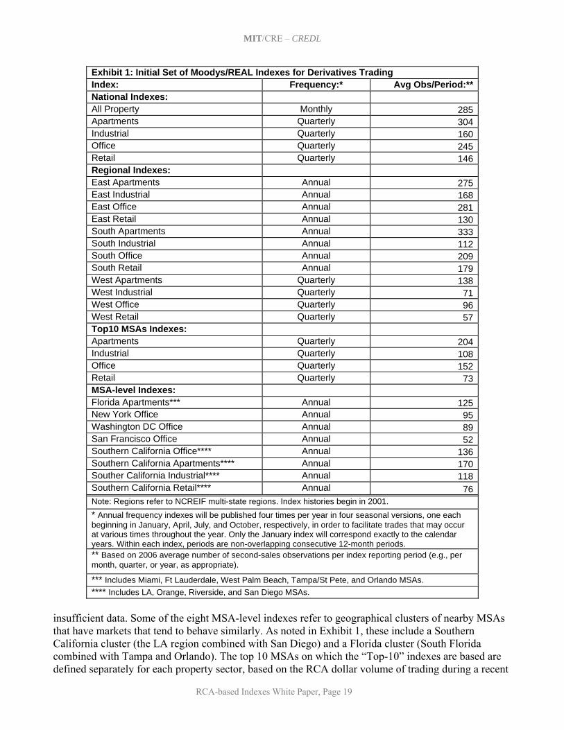
5. Initial Set of Indexes and Summary of Historical Results This section presents the set of same-property realized price-change indexes that have been developed to date based on the RCA transactions prices database, using the methodology described in Section 4. This set of indexes has been developed through an iterative process of consultation between the MIT/CRE research staff and the Project Advisory Team, based on the objectives and criteria noted in Section 3. The goal has been to produce a set of indexes that will support and facilitate the trading of derivatives based on them, such as index swap futures contracts. Which of these indexes are actually traded in the derivatives market will of course be determined only over time by the actual marketplace. In this section, we present and summarize the historical results to date of the major indexes. As the history of the indexes covers the period from the beginning of 2001 through the second quarter of 2007, the indexes trace a vivid picture of what has probably been one of the strongest “bull markets” in the history of U.S. commercial (investment) property markets. All of the actual historical returns of all of the indexes are presented in Appendix A at the end of this report. 5.1 A Basic Set of 29 Indexes The table in Exhibit 1 below presents the set of 29 basic indexes that will be published by Moody’s Investor Services beginning in 2007, together with their frequency and the recent data density in terms of the average number of second-sales observations per index reporting period during calendar year 2006. Of course, in principle, these 29 basic indexes can be combined and weighted in any number of ways by market participants and researchers for purposes of trading or analysis. It should be noted that there is no guarantee that the recent data density (number of transactions observations per period) will remain. On the other hand, the nature of repeat-sales databases is that they tend to grow rapidly in their early years as typical property holding periods between sales probably average close to 10 years. The RCA database only began coverage in 2000, and although there has been a concerted attempt by RCA to obtain prior sales information, the data density in the early years of the index history is much less than in recent years. For example, the National All-Property Index that averaged 285 second-sale observations per month in 2006 averaged only 29 such observations per month in 2001.* As is apparent in Exhibit 1, the present set of tradable indexes includes indexes at three geographical levels: national, regional, and MSA-level. In addition, a unique definition of the top 10 MSAs by recent trading volume grouped together (even though these are non-contiguous and located in various geographical regions) has been established to represent “primary markets” in which most large-scale or institutional real estate investment likely occurs. The national level is the only level at which an “All-Property” index aggregating all property usage type sectors is published, and this is the only index which at present is published at the monthly frequency. All other indexes pertain only to one of the four major commercial (income producing) property usage type sectors: apartments, industrial, office, and retail, as defined by RCA.† The multi-state regions on which the regional indexes are defined are the NCREIF regions, indicated in the map below Exhibit 1. It is not possible at present to publish any Midwest regional indexes due to

* The issue of data density will be discussed further in Section 6, regarding index publication protocols. † See the separate white papers available from RCA and Moody’s for detailed descriptions of property type sector and MSA level geographic regional definitions.

MIT/CRE – CREDL


Exhibit 1: Initial Set of Moodys/REAL Indexes for Derivatives Trading Index: Frequency:* Avg Obs/Period:**National Indexes: All Property Monthly 285Apartments Quarterly 304Industrial Quarterly 160Office Quarterly 245Retail Quarterly 146Regional Indexes: East Apartments Annual 275East Industrial Annual 168East Office Annual 281East Retail Annual 130South Apartments Annual 333South Industrial Annual 112South Office Annual 209South Retail Annual 179West Apartments Quarterly 138West Industrial Quarterly 71West Office Quarterly 96West Retail Quarterly 57Top10 MSAs Indexes: Apartments Quarterly 204Industrial Quarterly 108Office Quarterly 152Retail Quarterly 73MSA-level Indexes: Florida Apartments*** Annual 125New York Office Annual 95Washington DC Office Annual 89San Francisco Office Annual 52Southern California Office**** Annual 136Southern California Apartments**** Annual 170Souther California Industrial**** Annual 118Southern California Retail**** Annual 76Note: Regions refer to NCREIF multi-state regions. Index histories begin in 2001. * Annual frequency indexes will be published four times per year in four seasonal versions, one each beginning in January, April, July, and October, respectively, in order to facilitate trades that may occur at various times throughout the year. Only the January index will correspond exactly to the calendar years. Within each index, periods are non-overlapping consecutive 12-month periods. ** Based on 2006 average number of second-sales observations per index reporting period (e.g., per month, quarter, or year, as appropriate). *** Includes Miami, Ft Lauderdale, West Palm Beach, Tampa/St Pete, and Orlando MSAs. **** Includes LA, Orange, Riverside, and San Diego MSAs.

insufficient data. Some of the eight MSA-level indexes refer to geographical clusters of nearby MSAs that have markets that tend to behave similarly. As noted in Exhibit 1, these include a Southern California cluster (the LA region combined with San Diego) and a Florida cluster (South Florida combined with Tampa and Orlando). The top 10 MSAs on which the “Top-10” indexes are based are defined separately for each property sector, based on the RCA dollar volume of trading during a recent

MIT/CRE – CREDL


two year period. More indexes may be developed over time as the RCA database grows or methodological improvements are made.

5.2 Analysis of the National Aggregate Monthly Index The chart in Exhibit 2 shows the monthly National All-Property Index from 2001 through July 2007, in comparison with the NCREIF Property Index (NPI) during the same period (through June). It should be noted that both the Moodys/REAL and the NCREIF Indexes depicted here are “all-property” indexes, as distinct from weighted composites of sectoral indexes. This is a particularly important distinction in the transaction-based index, in that it treats all transactions as deriving from a single population of properties. The proportion of those transactions in different property sectors will vary over time.* The version of the NPI used in the comparison is the equal-weighted, cash flow based definition of the appreciation return index. This is the version of the NPI which is most directly comparable to the RCA-based indexes, because the RCA indexes are equally weighted across property transaction observations, and because the price changes depicted in the RCA indexes include the effect of capital improvement expenditures made to maintain the properties. This is also the case for the cash flow based version of the NPI.† * In principle, this could cause the index to more strongly reflect whichever property segments are trading more heavily at a given time. However, the repeat-sales methodology does not derive any periodic return based only on the transactions taking place in that period, but considers prior historical transactions as well in deriving each period’s return. In practice, we see no evidence that the national all-property index is overly influenced by “hot” sectors. If that were the case, its long-run average return would exceed that of the average across the sectors (unweighted), which is not the case. The geometric mean quarterly return in the all-property index for the 26 quarters 2001Q1-2007Q2 is 2.44%. Over that same period the unweighted average geometric mean return across the four national property sectors (apartment, industrial, office, retail) is 2.43%. This is in spite of the fact that different sectors clearly surged at different times. (See Section 5.3.) † In this respect, the price change indexes presented here are comparable to typical stock market share price indexes. Publicly traded corporations typically plow back some (or even all) of their earnings rather than paying them all out in dividends, in order to reinvest and “maintain” the corporation. Hence, stock share prices reflect the effect of capital improvement expenditures, and dividend yields are lower than earnings per share percentages.

MIT/CRE – CREDL


While the historical period depicted in Exhibit 2 has seen the strongest advance in NCREIF history, the NPI capital appreciation shown in Exhibit 2 is only 69% compared to 87% in the Moodys/REAL Index (from January 2001 through June 2007). This difference is probably due at least in part to the temporal lag in the NCREIF Index that is apparent in comparison to the RCA-based index in the chart.

Exhibit 2: Moodys/REAL Index Level Compared to NCREIF

0.8

0.9

1

1.1

1.2

1.3

1.4

1.5

1.6

1.7

1.8

1.9

2

Dec

-00

Apr

-01

Aug

-01

Dec

-01

Apr

-02

Aug

-02

Dec

-02

Apr

-03

Aug

-03

Dec

-03

Apr

-04

Aug

-04

Dec

-04

Apr

-05

Aug

-05

Dec

-05

Apr

-06

Aug

-06

Dec

-06

Apr

-07

Moodys/REAL(monthly)

NCREIF (qtrly)

Exhibit 2 suggests that the Moodys/REAL Index is able to more precisely detect movements in the market than the NPI, not only because of its monthly frequency (compared to the NPI’s quarterly frequency), but more importantly because a contemporaneous transactions-based index like the Moodys/REAL Index lacks the “smoothing” of an index constructed such as the NPI based on appraisals (as described in Section 1). The ability of the Moodys/REAL Index to detect market movements even in the index’s early days when data was scarce is apparent in the noticeable response to the 2001 recession that is apparent in the Moodys/REAL Index but not in the NPI. The RCA-based index also indicated some volatility and pausing in the bull market during part of 2006 before a particularly strong surge in early 2007, subtleties in market movements missed in the NPI.*

* In fact, 2006 saw the end of the condo and housing booms, and a temporary upsurge in interest rates (the 10-year T-bond yield increased from an average of almost 40 basis-points from 2005 to 2006). Early 2007 saw a fall-back in interest rates and the peak of the private equity surge including the hype surrounding the Blackstone buyout of Equity Office Properties. The real estate market transactions tracked by RCA (as quantified by the Moodys/REAL Index) show an asset market responding to these actual events and pressures, while the NPI seems much less responsive.

MIT/CRE – CREDL


While the temporal lead of the Moodys/REAL Index ahead of the NPI in part reflects the difference between the transactions-based versus appraisal-based index construction methodology, it also reflects some likely real difference in the behavior of the different types of properties tracked by the two indexes. As noted in Section 1, the NPI tracks only large, institutionally held properties (largely held directly or indirectly by pension funds), whereas the RCA-based Index is dominated by smaller properties that tend to be traded primarily by local private investors.*

Exhibit 3: Quarterly Capital Return Summary Statistics: Moodys/REAL and NCREIF, 2001Q1-2007Q2

Moodys/REAL NPI (EWCF) Mean 2.44% 2.03% Volatility 2.42% 1.93% Serial Correlation 9.77% 76.91% Cross-Correlation: 15.65%

Exhibit 3 (above) shows the summary capital returns statistics for the Moodys/REAL and the NCREIF Indexes computed on a quarterly frequency covering the 26 quarters from 2001 through June 2007. At this frequency over the historical period covered, the Moodys/REAL Index was only modestly more volatile than the NPI. The Moodys/REAL Index displayed only weak serial correlation, while the inertia in the NPI is apparent in its very high (over 76%) positive autocorrelation.† The two indexes were only slightly positively correlated on a contemporaneous basis. However, as Exhibit 4 reveals, the Moodys/REAL Index was much more strongly correlated with the subsequent (lagged) NCREIF Index, including +51% correlation still remaining with the NPI lagged three quarters later. Exhibit 5 compares a number of statistics of interest to investors between the Moodys/REAL Index and several other indexes or time series of investment interest at the quarterly frequency during the available 2001Q1-2007Q2 historical period. The comparison includes the MIT TBI (Transactions Based Index) which is a quarterly transactions-based (hedonic price model) index published by the MIT/CRE based on the NCREIF database. The TBI thus reflects the same institutional real estate as the NCREIF Index, but without the appraisal effects noted earlier. The NCREIF population tracked by

* There is some evidence that private local investors may tend to lead the rest of the property market. A thesis written at MIT in 2006 compared an RCA-based repeat-sales index based only on private local investor purchases versus a similar RCA-based index based on larger institutional purchases. The former tended to lead the latter slightly in time, though the historical sample was too short for statistical significance. (See J.H.Morrison, “An Analysis of Investor Types in Real Estate Capital Markets: Their Behavior & Performance 2000-2006”, MS Thesis, MIT, 2006.) † As noted in Section 4, strong positive autocorrelation in a capital returns series suggests sluggish or lagged incorporation of information, while strong negative autocorrelation suggests the presence of random error or excess volatility that is subsequently corrected.

MIT/CRE – CREDL


Exhibit 4: Correlation of Moodys/REAL with lagged NPI:

(Based on 22 to 26 quarterly returns: 2001-2007Q2) NPI lead 4 qtrs ahead of Moodys/REAL -24%NPI lead 3 qtrs ahead 14%NPI lead 2 qtrs ahead 0%NPI lead 1 qtr ahead 28%Contemporaneous 16%NPI lag 1 qtr behind Moodys/REAL 55%NPI lag 2 qtrs behind 36%NPI lag 3 qtrs behind 51%NPI lag 4 qtrs behind 30%

the TBI is a much smaller and narrower population of commercial properties than that tracked by the RCA-based index. As seen in the Exhibit, during the 2001Q1-2007Q2 period the Moodys/REAL Index displayed a modest 26% contemporaneous quarterly correlation with the TBI. However, the correlation is stronger between the Moodys/REAL Index and the TBI lagged. Not shown in the table is the 45% correlation between the RCA and the TBI lagged one quarter, and the additional 30% correlation between the RCA and the TBI lagged two quarters. This suggests that the small private investors who dominate in the RCA database have in some sense tended to move quicker than the institutions in the NCREIF database during most of the historical period covered. This is seen graphically in Exhibit 6, although we also note there some indication that very recently the institutional market may be surging ahead of (or beyond?) the broader market, as indicated by the TBI’s stronger surge during the latter half of 2006 and first half of 2007, the period coinciding with the peak of the private equity boom, including the buyout of several major REITs. The Moodys/REAL Index showed little contemporaneous correlation with the other series in the Exhibit 5. While the Moodys/REAL Index showed only a modest 33% correlation with inflation, this was the highest of any of the series shown in the table. The Moodys/REAL volatility was only modestly above the appraisal-based NPI, which made it low compared to both long-term bonds and the TBI, and very low compared to both REITs and the broader stock market. The RCA-based index displayed virtually no “beta” with respect to the S&P500 large-cap stock index, confirming (at least for 2001Q1-2007Q2) the conventional wisdom that commercial real estate offers attractive diversification characteristics in a mixed-asset portfolio dominated by stocks and bonds. Of particular interest is also the relationship between the Moodys/REAL Index and the NAREIT Index of equity REIT share price capital returns. The statistical comparison is included in Exhibit 5 (quarterly through 2007Q2), and the chart in Exhibit 7 depicts the cumulative price indexes (monthly through end of July 2007). While the two indexes display the same pattern at the broad-brush level, notably a tremendous run up in prices, or “bull market”, the specifics are rather different over the short to medium term. The REIT-based index is much more volatile than the direct property index at the quarterly frequency (7.34% versus 2.42% quarterly volatility), and the two indexes showed no significant correlation at this frequency during the 2001Q1-2007Q2 period (14% contemporaneous correlation). The NAREIT Equity REIT index showed somewhat greater price appreciation than the direct commercial property market tracked by the Moodys/REAL Index during the 2001Q1-2007Q2 period, with a 2.88% versus 2.44% per quarter geometric mean return. It is interesting that, unlike

MIT/CRE – CREDL


Exhibit 5: Summary Statistics for Quarterly Capital Returns for Eight Series of Interest, 2001Q1-2007Q2 (26 obs) Moodys/

REAL TBI NPI NAREIT

(Equity) CPI

Inflation* T-Bills* LTG

Bond* S&P500

* Mean 2.44% 2.68% 2.03% 2.88% 0.66% 0.66% 0.31% 0.29%

Volatility 2.42% 4.32% 1.93% 7.34% 0.91% 0.39% 4.42% 8.22% Serial Correlation 9.77% 1.42% 76.91% -25.86% -40.52% 93.80% -24.99% -15.92%

Beta wrt S&P 0.00 0.12 0.05 0.48 -0.04 -0.01 -0.22 1.00 Correlations:

Moodys/REAL 100% 26% 16% 14% 33% -6% 11% 0% TBI 26% 100% 65% 15% 1% 15% 15% 23% NPI 16% 65% 100% 12% 6% 40% 0% 21% NAREIT (Eq) 14% 15% 12% 100% -17% 0% -5% 59% CPI Infla* 33% 1% 6% -17% 100% 9% -23% -33% T-Bills* -6% 15% 40% 0% 9% 100% -8% -14% LTG Bond* 11% 15% 0% -5% -23% -8% 100% -43% S&P500* 0% 23% 21% 59% -33% -14% -43% 100% * CPI Infla, 30-day T Bills, LT Govt Bonds, and S&P500 from Ibbotson Associates. Note that the CPI is not a "return", but simply the current rate of inflation. The T-Bill return is a total return as defined by Ibbotson (but largely the same as the average going-in yield for 30-day bills).

Exhibit 6: Moodys/REAL Index Compared to MIT TBI Index

0.8

0.9

1

1.1

1.2

1.3

1.4

1.5

1.6

1.7

1.8

1.9

2

2.1

Dec

-00

Apr

-01

Aug

-01

Dec

-01

Apr

-02

Aug

-02

Dec

-02

Apr

-03

Aug

-03

Dec

-03

Apr

-04

Aug

-04

Dec

-04

Apr

-05

Aug

-05

Dec

-05

Apr

-06

Aug

-06

Dec

-06

Apr

-07

Moodys/REAL(monthly)

MIT TBI (qtrly)

MIT/CRE – CREDL


the temporal relationship between the RCA-based index and the other real estate indexes discussed above, there is no clear lead or lag relationship between the RCA-based index and the NAREIT Equity REIT index.

Exhibit 7: Moodys/REAL Index Compared to NAREIT

0.80.9

11.11.21.31.41.51.61.71.81.9

22.12.22.32.42.52.6

Dec

-00

Apr

-01

Aug

-01

Dec

-01

Apr

-02

Aug

-02

Dec

-02

Apr

-03

Aug

-03

Dec

-03

Apr

-04

Aug

-04

Dec

-04

Apr

-05

Aug

-05

Dec

-05

Apr

-06

Aug

-06

Dec

-06

Apr

-07

Moodys/REAL

NAREIT (equityREITs price)

Both indexes set to equal 1.0 in Dec 2000, and compared through July 2007.

It should be noted that both the similarities and differences between the Moodys/REAL and NAREIT-based indexes noted in the preceding paragraph make sense. We would not expect an index based directly on commercial property prices in the private market to behave very similarly to a REIT-based index in the short to medium term, for a variety of reasons. REITs are levered, whereas the RCA transaction prices are at the property (unlevered) level. During a market upswing, this would cause REIT share prices to tend to grow more rapidly, and generally to display greater volatility.* Of course, the specific properties whose price changes are represented in the Moodys/REAL Indexes are for the most part different from the properties held by the REITs tracked by the NAREIT Index (although when REIT properties are bought and sold these transactions will normally be picked up in the RCA database†).

* And of course the levels should not be compared across the two indexes, as they both are set arbitrarily equal to 1.00 in December 2000. † A major exception being portfolio transactions in which the prices of individual properties cannot be sorted out to allow reliable paired-sale price comparisons, per Filter #II described in Section 4.3.

MIT/CRE – CREDL


Even more important, REITs are vertically integrated real estate operators and active investment players whose management at the entity level can importantly determine the performance of the firm. REITs don’t just passively hold a static portfolio of properties, but actively buy, sell, and develop properties, as well as land, and engage in a variety of tenant services and other activities (including taxable REIT subsidiary activities). It is also important not to underestimate the fact that REIT share prices reflect the valuation of the stock market, which may differ from that of the private property market, as the functioning and investor clienteles differ across these two very different types of capital asset markets.* On the other hand, REITs are fundamentally, primarily commercial property investment plays, and over the long run and in the big picture, we would expect a REIT index and a direct commercial property price index to be substantially related. The picture presented by Exhibits 5 and 7 is not at all inconsistent with such a relationship.

5.3 The National Property Type Sector Indexes The quarterly return statistics for the Moodys/REAL national property type sector indexes are summarized in Exhibit 8, and the indexes are displayed graphically in Exhibit 9, for the available history from 2001 through the second quarter of 2007. During this historical period the geometric mean return ranged from 2.23%/quarter for office, to 2.59% for apartments, while the quarterly volatility ranged from over 2% for retail to almost 4% for apartments and industrial. The first-order autocorrelations are generally influenced by the operation of the ridge noise filter (see discussion in Section 4.2.2†), so the 4th-order autocorrelations are also shown in Exhibit 8. These autocorrelations, as well as the cross-correlations shown in the bottom part of the table, and the visual appearance of the indexes in Exhibit 9, are consistent with what one would expect in relatively noise-free indexes.‡ Excessive noise would be indicated by high negative autocorrelations, zero cross-correlations, and a “choppy” or “sawtooth” appearance in a graph of the index levels.§ Note in Exhibit 9 that while all four property type sectors have broadly moved together during the 2001Q1-2007Q2 period, and all have shared in the great bull market, there are some noteworthy differences. The office sector suffered worst from the recession in 2001-2002. More recently, the * Prominent in Exhibit 7 is the 17% decline in REIT share prices during June and July 2007. This may signal a turning point in the private commercial property market as well, although through the end of July the Moodys/REAL Index had picked up only an end to the “surge” of early 2007 (an end to the spike after the 2006 pause in the 3-year bull market); not as yet any clear indication of a downturn. In May 2007, coinciding with an up-tick in interest rates, the Moodys/REAL Index dropped slightly, and between April and end of July was essentially flat (gained less than 1%), while the NCREIF Index was showing no sign of a pause in its growth (up 4% in the second quarter after less than 3% growth in the first quarter) and the NAREIT Index was plunging the aforementioned 17% during this time. † The noise filter cannot be used to decrease a 1st-order autocorrelation which already exceeds zero without the filter, as was the case with the office index in this instance. ‡ This is not to say that there is no noise at all in the indexes. We would expect to see greater positive cross-correlation among the sectors, at least over the long run, and this will likely show up over time and in lower frequency returns. (For a given index, the signal/noise ratio will be higher in longer interval returns.) While there is not yet sufficient historical data to rigorously analyze the degree of noise present in the Moodys/REAL sectoral indexes, we are comforted not only by the appearance of the indexes in Exhibit 9, but also by the relative stability and robustness of the way these indexes have appeared across several iterations and updatings of developmental databases supplied to MIT by RCA. § It should be noted that noise can be “masked” (eliminating some of the indications noted here) without being eliminated, through the use of certain types of smoothing techniques (which introduce a lag bias), such as the use of overlapping rolling or moving-average returns. Such techniques are not employed in the Moodys/REAL indexes.

MIT/CRE – CREDL


apartment sector, after growing the fastest in 2004-2005, suffered a correction during late 2005-2006 as it digested the end of the condo conversion boom, until picking up again since the fourth quarter of 2006 in most regions of the country.

Exhibit 8: Moodys/REAL National Property Sector Indexes, Quarterly Capital Returns Statistics: 2001Q1-2007Q2 (26 obs)

Apartments Industrial Office RetailMean 2.59% 2.40% 2.23% 2.50%Volatility 3.86% 3.65% 3.17% 2.37%1st-order Autocorrelation -2.25% 2.91% 22.16% -5.07%4th-order Autocorrelation -21.87% 8.12% 25.70% 12.16%Cross-Correlation: Apartments 100% 30% -19% 14%Industrial 30% 100% 5% -2%Office -19% 5% 100% 41%Retail 14% -2% 41% 100%

Exhibit 9: Moodys/REAL National Sectoral Indexes

0.9

1.0

1.1

1.2

1.3

1.4

1.5

1.6

1.7

1.8

1.9

2.0

4Q 2

000

2Q 2

001

4Q 2

001

2Q 2

002

4Q 2

002

2Q 2

003

4Q 2

003

2Q 2

004

4Q 2

004

2Q 2

005

4Q 2

005

2Q 2

006

4Q 2

006

2Q 2

007

Apartments

Industrial

Office

Retail

MIT/CRE – CREDL


5.4 The Regional and MSA-level Indexes The regional and MSA levels of the Moodys/REAL Indexes are presently intended to be published primarily at the annual frequency, due to data availability considerations.* The only exception is the West region, which is able to publish at the quarterly frequency. All four property sectors are published for the three NCREIF regions that are covered: East, South, and West. It is not possible at present to publish Midwest indexes. As the RCA database grows in the future, this may change. In addition, eight MSA-level indexes are to be published at present. These include all four property sectors for the Southern California MSA cluster (LA and San Diego), plus three office sectoral indexes for New York, Washington DC, and San Francisco, and an apartment sector index for a Florida MSA cluster consisting of an aggregation of Miami, Ft Lauderdale, West Palm Beach, Tampa/St Pete, and Orlando. Exhibits 10 and 11 below present summaries of the four quarterly West region sectoral indexes. The statistics in the table in Exhibit 10 are similar to the national level sectoral indexes statistics discussed previously, and the patterns apparent in the chart in Exhibit 11 are also similar. The most notable distinctions are the more negative performance of the West office sector during the 2001-2003 period as much of the West Coast (especially the San Francisco area) struggled with the aftermath of the tech bubble. There was also particularly strong and steady performance of West Region retail until the past year when it alone among the sectors appears to have paused.

Exhibit 10: West Region Quarterly Return Statistics by Sector, 2001Q1-2007Q2 (26 obs)

Apartments Industrial Office Retail Mean 2.63% 2.18% 1.97% 2.55% Volatility 3.27% 3.20% 5.71% 2.24% 1st-order Autocorrelation 10.27% 17.61% -7.39% 26.63% 4th-order Autocorrelation 12.91% 10.89% 3.28% -11.97% Correlations: Apartments 100% 36% -7% -7% Industrial 36% 100% 30% 18% Office -7% 30% 100% 18% Retail -7% 18% 18% 100%

________________________ * See Appendix D at the end of this white paper for a description of a methodology which can be used to derive implied quarterly frequency returns from the staggered annual indexes. In the future, publication of such derived quarterly returns indexes may be considered.

MIT/CRE – CREDL


Exhibit 11: Moodys/REAL West Region Property Sector Indexes

0.7

0.9

1.1

1.3

1.5

1.7

1.9

2.1

4Q 2

000

2Q 2

001

4Q 2

001

2Q 2

002

4Q 2

002

2Q 2

003

4Q 2

003

2Q 2

004

4Q 2

004

2Q 2

005

4Q 2

005

2Q 2

006

4Q 2

006

2Q 2

007

ApartmentsIndustrialOffice Retail

MIT/CRE – CREDL


Exhibit 12: Moodys/REAL Indexes East and South Regions Annual Capital Returns Statistics 2001-2007 (FYJ Indexes Yrs Ending June, 6 obs)

East Apts South

Apts East

Indust South Indust

East Office

South Office

East Retail

South Retail

Mean 12.61% 8.32% 9.83% 11.06% 10.00% 9.81% 12.45% 10.43% Volatility 12.26% 15.90% 9.20% 7.57% 4.90% 9.03% 8.16% 6.84% Autocorrelation -41.4% -16.5% -5.2% 20.7% 15.2% -18.4% -21.7% 10.0% Correlation:

East Apts 100% 91% 84% 52% 37% 45% 65% 61% South Apts 91% 100% 98% 74% 58% 53% 65% 84%

East Indust 84% 98% 100% 70% 60% 40% 70% 89% South Indust 52% 74% 70% 100% 65% 69% 32% 75%

East Office 37% 58% 60% 65% 100% 11% -6% 37% South Office 45% 53% 40% 69% 11% 100% 16% 53%

East Retail 65% 65% 70% 32% -6% 16% 100% 75%South Retail 61% 84% 89% 75% 37% 53% 75% 100%

Exhibit 12 summarizes the historical return statistics for the East and South Regions by property sector. These indexes are produced at the annual frequency, and the annual return statistics shown in the table are based on the Fiscal Year ending June (FYJ indexes), and thus cover the six annual returns fom the period from July 1st 2001 through June 30th 2007. As noted, there are three other versions of the annual indexes, beginning in each of the other three quarters, so as to facilitate trading at various times during the year.* With only six return observations, we should not make too much of the statistics shown in the table. (Indeed, the short history raises a major caveat concerning all of the index second moment statistics reported throughout Section 5.) Nevertheless, it is worth noting that the cross-correlations among the various indexes in Exhibit 12 are generally rather large. This suggests that the indexes do not suffer from much statistical noise. The magnitude of the within-sector correlations, highlighted along the diagonal of the correlation matrix, make intuitive sense. The graphical depictions of these indexes in Exhibits 13 and 14 reveal a generally steady upward climb during the historical period, with the fastest growth during 2004-2005. The exceptions are the two apartment indexes, which begin to turn down in 2006 (this would be from late 2005 in the FYJ indexes). _______________ * As noted, within each index, the annual periods are non-overlapping and “independent” (from a statistical perspective).

MIT/CRE – CREDL


Exhibit 13: Moodys/REAL East Region Property Sector Indexes

0.91.01.11.21.31.41.51.61.71.81.92.02.1

2001 2002 2003 2004 2005 2006 2007

East Apts

East Indust

East Office

East Retail

Exhibit 14:

Moodys/REAL South Region Property Sector Indexes

0.91.01.11.21.31.41.51.61.71.81.92.02.1

2001 2002 2003 2004 2005 2006 2007

South Apts

South Indust

South Office

South Retail

The table in Exhibit 15 presents the annual return summaries for the eight MSA-level indexes, again based on the FYJ version of these annual indexes (ending in June). As before, great caution should be used in reading too much into statistics based on only six annual returns. The graphical depictions of the MSA-level market movements in the charts in Exhibits 16, 17, and 18 may be more instructive and intuitive.

MIT/CRE – CREDL


Exhibit 15: Moodys/REAL Indexes MSA-level Annual Capital Returns Statistics 2001-2007 (FYJ Indexes Yrs Ending June, 6 obs)

FL Apts SoCal

Apts SoCal Indust

SoCal Retail

SoCal Office SF Office

NYC Office DC Office

Mean 13.67% 13.58% 13.11% 16.01% 10.77% 4.10% 14.43% 9.53%Volatility 15.68% 7.19% 7.59% 5.30% 9.36% 8.86% 3.95% 4.42%Autocorrelation -1.8% 75.8% 60.7% -33.3% 32.4% 88.0% -0.5% -3.9%Correlation FL Apts 100% 47% 57% 75% 60% 5% 22% 99%SoCal Apts 47% 100% -39% 45% 24% -61% -64% 37%SoCal Indust 57% -39% 100% 41% 61% 73% 63% 66%SoCal Retail 75% 45% 41% 100% 42% -24% -9% 74%SoCal Office 60% 24% 61% 42% 100% 46% -14% 59%SF Office 5% -61% 73% -24% 46% 100% 55% 17%NYC Office 22% -64% 63% -9% -14% 55% 100% 32%DC Office 99% 37% 66% 74% 59% 17% 32% 100% Exhibit 16 depicts the four property sectors all within the Southern California MSA cluster. The star performer during 2001-2007 was the retail sector, while the weakest sector (though still strong) was office, due to a slow start early in the decade and only modest growth in 2006. Exhibit 17 depicts the four MSA-level office indexes: New York, Washington DC, San Francisco, and Southern California. The odd man out in this grouping is San Francisco, whose office market at first declined in response to the bursting of the tech bubble and the recession of 2001-2002, and has since recovered but not nearly as strong as the other three markets. Finally, Exhibit 18 shows the two MSA-level apartment markets currently being tracked: the Florida and Southern California MSA clusters. Notable is the 2005 boom in South Florida apartment values as the condo-conversion phenomenon peaked in Florida in that year, followed by the sharp downturn in 2006-07 as the condo market declined.

MIT/CRE – CREDL


Exhibit 16: Moodys/REAL Southern California Sector Indexes

0.8

1.0

1.2

1.4

1.6

1.8

2.0

2.2

2.4

2.6

2001 2002 2003 2004 2005 2006 2007

SoCAL Apts

SoCAL Indust

SoCAL Office

SoCAL Retail

Years ending June 30.

Exhibit 17: Moodys/REAL Office Sector Indexes in 4 MSAs

0.8

1.0

1.2

1.4

1.6

1.8

2.0

2.2

2.4

2001 2002 2003 2004 2005 2006 2007

SoCAL

SF

NY

DC


MIT/CRE – CREDL


Exhibit 18: Moodys/REAL Apartment Sector Indexes in 2 MSAs

0.9

1.1

1.3

1.5

1.7

1.9

2.1

2.3

2001 2002 2003 2004 2005 2006 2007

SoFL

SoCALl


As noted, the annual indexes are all produced in four seasonal cohorts, staggered so that their years begin one quarter after the previous index. As a visual illustration of this procedure, Exhibit 19 shows all four of the staggered annual indexes for the example case of the Southern California Apartments index. The January-based CY index corresponds to calendar years. The other indexes are based at the beginning of each of the subsequent calendar quarters: April, July, and October. Thus, the last annual index cohort depicted in Exhibit 19 is the July-based FYJ index that defines annual returns based on years running from July 1st through June 30. As noted, within each index the annual returns are non-overlapping in time. Each index therefore presents returns that are statistically independent within the index, and does not contain any smoothing or lagging that would result from such overlapping or taking a rolling moving-average. In Exhibit 19 all of the four staggered annual indexes are set to start arbitrarily at a value of 1.00. Of course, this is inconsistent with the implication of the first annual returns indicated by each of the indexes. If one were to set the starting value of each index at a level implied by the first year returns indicated by the index cohorts that started earlier, one would gain a better visual composite picture of what the indexes imply about the market’s history. However, such overlapping of annual indexes could present a misleadingly smooth appearance, and might not reveal a turning point when it first occurs. For example, all of the annual returns in Exhibit 19 are positive, including the most recent four: the FYS 2006, CY 2006, FYM 2007, and FYJ 2007. At first you might think this implies that the Southern California apartment market has not yet shown any evidence of a turning in the market. And if you superimposed the four annual indexes on top of one another a very smooth upward trend would indeed appear, with only a tapering near the end. But consider that the FYS 2006 return for the 12 months ending in September 2006 was +9.0%, while the CY 2006 return for the 12 months ending only three months later in December 2006 was only +2.6%. This suggests that the fourth quarter of 2006 may have actually seen a slight downturn in the Southern California apartment market. The subsequent

MIT/CRE – CREDL


annual returns ending in March and June of 2007, coming in at rates of 2.0% and 1.7% respectively, would seem to confirm that 2006Q4 was a turning point or at least the beginning of a plateau in the Southern California apartment market. As noted, a procedure for deriving implied quarterly returns from the staggered annual indexes in a manner that can pick up these types of turning point indications is presented in Appendix D at the back of this report.

Exhibit 19: Four Annual Southern California Apartment Indexes Based on Four Different Base Months

0.8

1

1.2

1.4

1.6

1.8

2

2.2

2.4

2.6

4Q 2

000

2Q 2

001

4Q 2

001

2Q 2

002

4Q 2

002

2Q 2

003

4Q 2

003

2Q 2

004

4Q 2

004

2Q 2

005

4Q 2

005

2Q 2

006

4Q 2

006

2Q 2

007

CY (Yr Ending Dec)FYM (Yr Ending Mar)FYJ (Yr Ending Jun)FYS (Yr Ending Sep)

5.5 The Top-10 MSAs Indexes In addition to the above-described indexes which are either national or specific to contiguous geographic regions, the Moodys/REAL Indexes will also include a set of four property sector specific indexes based on the 10 largest MSAs (together) for each property sector, where “largest MSAs” is defined based on the RCA total trading dollar volume within each sector during the preceding 24 months. The MSAs included in the top 10 will be reexamined and possibly changed once every two years (or as subsequently determined by Moodys), according to a specific schedule to be determined by Moodys, based on the trading volume during the preceding two years. Any such changes will be announced in advanced and applied on a going-forward basis only. The initial Top-10 Indexes are based on RCA trading volume during 2005 and 2006, including the metro areas listed in Exhibit 20 in each sector (listed in alphabetical order). In each sector the top 10 MSAs listed here represent at least 40% to 60% of the total national trading volume reported by RCA in 2005-2006.

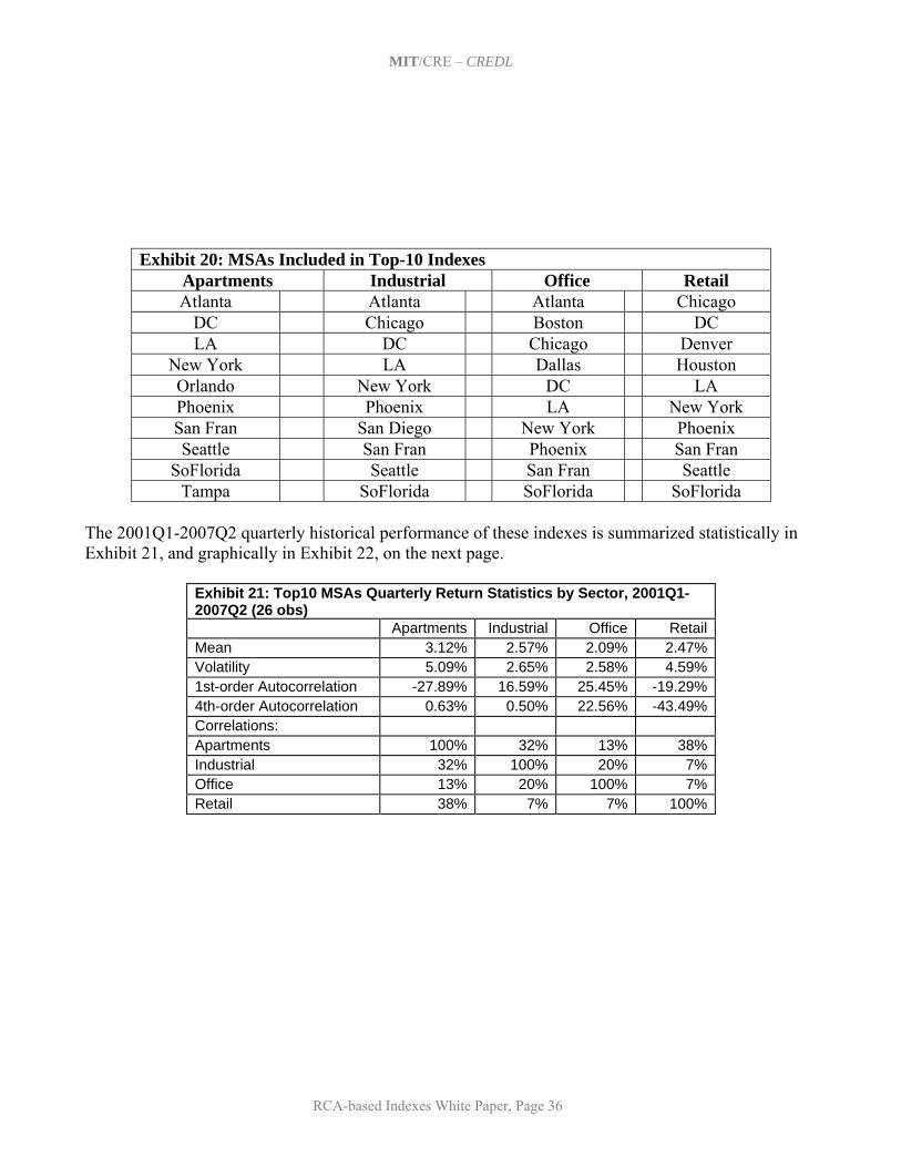
MIT/CRE – CREDL


Exhibit 20: MSAs Included in Top-10 Indexes Apartments Industrial Office Retail Atlanta Atlanta Atlanta Chicago

DC Chicago Boston DC LA DC Chicago Denver

New York LA Dallas Houston Orlando New York DC LA Phoenix Phoenix LA New York San Fran San Diego New York Phoenix Seattle San Fran Phoenix San Fran

SoFlorida Seattle San Fran Seattle Tampa SoFlorida SoFlorida SoFlorida

The 2001Q1-2007Q2 quarterly historical performance of these indexes is summarized statistically in Exhibit 21, and graphically in Exhibit 22, on the next page.

Exhibit 21: Top10 MSAs Quarterly Return Statistics by Sector, 2001Q1-2007Q2 (26 obs)

Apartments Industrial Office Retail Mean 3.12% 2.57% 2.09% 2.47% Volatility 5.09% 2.65% 2.58% 4.59% 1st-order Autocorrelation -27.89% 16.59% 25.45% -19.29% 4th-order Autocorrelation 0.63% 0.50% 22.56% -43.49% Correlations: Apartments 100% 32% 13% 38% Industrial 32% 100% 20% 7% Office 13% 20% 100% 7% Retail 38% 7% 7% 100%

MIT/CRE – CREDL


Exhibit 22: Moodys/REAL Top10 MSAs Property Sector Indexes

0.91.0

1.11.21.31.4

1.51.61.7

1.81.92.02.1

2.22.3

4Q 2

000

2Q 2

001

4Q 2

001

2Q 2

002

4Q 2

002

2Q 2

003

4Q 2

003

2Q 2

004

4Q 2

004

2Q 2

005

4Q 2

005

2Q 2

006

4Q 2

006

2Q 2

007

Apartments

Industrial

Office

Retail

MIT/CRE – CREDL


6. Protocols of Index Production and Publication: Practical Considerations for a Tradable Index Unlike property market price indexes designed primarily for research or academic purposes, the Moodys/REAL indexes described in this report are designed to support derivative trading in a practical manner. With this in mind, consultation between the MIT/CRE research staff and the Project Advisory Team has led to certain protocols regarding the operational production and publication of the indexes. These protocols will be described in this section, regarding delay of index reporting to allow for accumulation of data, and regarding contingencies in the event of insufficient data for specific indexes. In both cases, the specific protocols presented here represent initial policies deemed useful to facilitate the commencement of derivative trading. Like the index methodology described in Section 4, these production and publication protocols will be subject to periodic review. The goal is to provide indexes that are the most practical and useful possible for the derivatives marketplace. As noted, this represents a type of “engineering” project, to devise a practical tool for the stated purpose, rather than a purely academic exercise. Both the index methodology described in Section 4 and the production protocols described in this section have not been optimized from a purely econometric perspective, but rather reflect a balance of econometric and practical trading considerations. 6.1 Index Reports: Time Allowed to Gather Price Data We want the index return in a given period to represent as well as is practically possible the change in realized same-property prices up to the end of that period, as evidenced by second-sale transactions actually closed prior to and during the subject period. Yet it takes time for the prices of closed transactions to be recorded and reported, and to be gathered and compiled by RCA, and the derivatives market places a value on timely closing of contracted positions. Experience with the developmental database suggests that within 45 to 75 days of the close of an index reporting period, a sufficient quantity and proportion of the second-sale transactions that RCA will ultimately gather from the given month will be available for index construction. Based on this consideration, for indexes where the data availability is sufficiently dense (generally, the monthly and quarterly indexes), 45 days will be allowed to elapse after the end of the reporting period to accumulate data for index computation. For indexes where the data availability is less dense (generally the annual indexes), 75 days will be allowed to elapse. In all cases, the index report will be considered to be final once it is published, and any second sales occurring beyond the end of the subject period will be excluded from the index computation (no “backward adjustment”). This protocol for reporting of the index returns is aimed at striking a balance between maximizing data usage and providing a base for rapid, real-time closure of trades upon the indexes. The vast majority of the second-sales occurring by the end of the subject period that will ever be in the RCA database will normally be incorporated within the 45 and 75-day windows described above.

6.2 Contingencies for Temporary Loss of Sufficient Data: What to do when a market “dries up” As noted in our discussion of methodology in Section 4.2, any real estate price index will contain some “noise”, or excess randomness. The more second-sale observations available in any given index reporting period, the less such noise is likely to be present. Even though the indexes are based on only and all actual transaction price data that has passed through RCA’s data qualification and validation process as well as the filtering screens and the return estimation optimization and noise-control

MIT/CRE – CREDL


methodology described in Section 4, there can arrive a point of diminishing data availability at which the danger of too much noise becomes large enough that some contingency for such situations has been deemed desirable. The contingency that will be employed in the initial Moodys/REAL Indexes is described in this section. The indexes which have been established for initial publication for trading purposes, as described in this paper, have been based on the following simple criterion. If the second-sale transaction observation data frequency observed in CY 2005 were to fall by a factor of one-half, there would still be at least approximately 20 observations per quarter for directly computed quarterly indexes and 40 observations per year for the annual indexes. Exhibit 23 shows the data frequency and the ratio of sample size to the minimum criterion noted above during CY 2006.* The only index that appears somewhat marginal based on the 2006 data frequency is the San Francisco MSA office index. However, we feel that all of the indexes established at this time are important enough, and close enough to the criterion, to warrant publication of these indexes. The particular criterion of 20 and 40 observations per period as half of the 2005 observation frequency is admittedly ad hoc from a rigorous econometric perspective. This criterion has been set based on the judgment and experience of the MIT/CRE principal investigators (David Geltner and Henry Pollakowski), in consultation with the Project Advisory Team, and based on analysis of the behavior of proto-type RCA-based indexes when data is sparse (including potential indexes which we have decided not to publish for now). The decision to publish an index for the purpose of derivative trading is not to be taken lightly, because once the index commences publication, and contracts are possibly written on it, the publication of the index must continue. The decision to publish any given set of indexes is naturally a subjective balance between the objective of minimizing noise in any published index return versus the objective of providing the derivatives market with as many “market-specific” indexes as possible. We cannot guarantee that the published indexes will never exhibit noisy or anomalous returns.† Nor can we state exactly how frequently, if ever, the criterion values of 20 or 40 observations will be breached. In the event that any index in any period falls below the criterion data frequency (20 observations for direct quarterly frequency, 40 for derived quarterly frequency), the following procedure has been agreed upon. The subject index will be combined with the same sector index at the next higher level of geographic scope, with the subject index weighted in proportion to the number of observations as a percentage of the criterion amount. Thus, for example, suppose in a given year the New York MSA

* The RCA database registered fewer observations during 2006 than during 2005 in some markets, resulting in the ratios in Exhibit 23 being in some cases below the 2.0-times factor which guided the original index establishment based on 2005 data frequency. † Noise caused by sparse observations would tend to show up as spurious or anomalous returns. The nature of this type of noise is that it tends to correct itself in the next reported return (spurious returns have strong negative first-order autocorrelation), and the noise does not accumulate over time (spurious returns have zero autocorrelation after the first subsequent period). Thus, the longer the time span over which a return is measured (the greater the number of return reporting periods), the less impact random noise will have.

MIT/CRE – CREDL


Office Index has only 30 second-sale observations, which is less than the 40-observation criterion. In that case the New York Office Index will be derived as follows:*

NY Off Return = (30/40)*(Original NY Off Return) + (10/40)*(East Region Off Return). While the likelihood of the need to use this contingency protocol is considered small, derivative traders writing contracts on these indexes must be aware of this policy and must take it in consideration when they write their contracts. Commercial real estate markets tend to be strongly pro-cyclical in transaction volume. During a severe market downturn, transaction volume, and hence price observations, could fall substantially from recent levels. On the other hand, RCA continues to increase its scope and depth of data collection, and it is in the inherent nature of repeat-sales databases to grow substantially in the early years, as properties are typically held on average 10 years between sales. Note in Exhibit 23 that most of the indexes could experience a data reduction of one-half compared to the 2006 levels, in some cases much more than one-half, before they would fall below the criterion observations frequency. The table shows the data density (net of filters) as of 2006 for the individual regional and MSA level indexes. The indexes that would appear to be in the most danger of falling below the criteria include the New York, Washington DC, and San Francisco MSA office indexes, and the Southern California retail index. It is important to note that the criterion values of 20 or 40 observations per period are not “magic numbers”. As noted, it is not impossible for an anomalous or spurious return to occur even when there is more data than this, nor is it necessarily the case that returns reported with less than the criterion data will be anomalous. In our experience, the indexes can behave reasonably even with less than the criterion amount of data. Any published index report will be based on actual realized same-property price changes insofar as is reasonably possible to eliminate any data errors, and based on ALL of the available data (net of the previously-described data filters). As described in Appendix C, the repeat-sales model does not derive the returns for the current period (or any period) based only on the sales that occur in that period, but in fact uses directly or indirectly all of the prior historical price observations. Exhibit 24 presents some information that may be relevant in the event of the need to use the data scarcity contingency described in this section. The table reveals that while correlations over the 2001-2007 period have generally been positive between the lower level and higher level indexes, often strongly positive, there are cases where the correlation was weak. The average within-sector correlation between regional and national indexes is 60%, and the average within-sector correlation between MSA-level and regional indexes is 63%. However, it is difficult to gain much knowledge about these correlations from this short historical sample. Comparison of the MSA-level index charts

* Suppose the next higher geographic level index also has less than the criterion quantity of observations (an extremely unlikely occurrence). Then the procedure will be to combine the subject, the next higher, and the national level index for the subject sector. For example, suppose the New York Office Index has only 10 observations (with 40 as the criterion), and the East Office Index (for the same year) has only 30 observations (including the 10 in New York, which is still less than the 40 criterion). Then the weighting would be as follows: (10/40)*(30/40) = (3/16) on the original New York index; (30/40)*(30/40) = (9/16) on the East Office Index; and (1 – 3/16 – 9/16) = (16-12)/16 = (1/4) on the National Office Index. If there still isn’t the criterion number of observations even at the national level, then the subject index will not be published for the given period, but instead that “period” will be “extended” to include the subsequent period combined together. Any of the eventualities described in this footnote are considered to be extremely unlikely, except possibly in the event of a major catastrophe such as Hurricane Katrina in New Orleans.

MIT/CRE – CREDL


in Exhibits 16, 17 and 18 with the corresponding same-sector indexes in the charts in Exhibits 11, 13, and 14, suggests that there are no major differences between the MSA and Regional indexes.

Exhibit 23: 2006 Average Second-Sale Observations Per Index Reporting Period Compared to Criterion Value

2006 Avg Obs/Period

Criterion Value

Ratio Obs/Criterion

Regional Indexes: East Apts (Derived Qtrly) 275 40 6.9East Indust (Derived Qtrly) 168 40 4.2East Office (Derived Qtrly) 281 40 7.0East Retail (Derived Qtrly) 130 40 3.3South Apts (Derived Qtrly) 333 40 8.3South Indust (Derived Qtrly) 112 40 2.8South Office (Derived Qtrly) 209 40 5.2South Retail (Derived Qtrly) 179 40 4.5West Apts (Qtrly) 138 20 6.9West Indust (Qtrly) 71 20 3.5West Office (Qtrly) 96 20 4.8West Retail (Qtrly) 57 20 2.9

Top10 MSAs Indexes: Apartments (Qrtly) 204 20 10.2Industrial (Qrtly) 108 20 5.4Office (Qtrly) 152 20 7.6Retail (Qrtly) 73 20 3.6

MSA-level Indexes (Derived Qtrly): Florida Apts* 125 40 3.1New York Office 95 40 2.4DC Office 89 40 2.2SF Office 52 40 1.3SoCal Office** 136 40 3.4SoCal Apts** 170 40 4.3SoCal Indust** 118 40 3.0SoCal Retail** 76 40 1.9* Includes Miami, Ft Lauderdale, West Palm Beach, Tampa/St Pete, and Orlando MSAs. ** Includes Los Angeles area and San Diego MSAs.

MIT/CRE – CREDL


Exhibt 24: Correlation of Regional and MSA Level Indexes with Same-Sector Next Higher Geographic Level Index

Regional Indexes: Correlation with

National***: East Apts (Annual) 63% East Indust (Annual) 70% East Office (Annual) 80% East Retail (Annual) 26% South Apts (Annual) 65% South Indust (Annual) 72% South Office (Annual) 27% South Retail (Annual) 58% West Apts (Qtrly) 75% West Indust (Qtrly) 76% West Office (Qtrly) 42% West Retail (Qtrly) 67% AVERAGE Regional 60%

MSA-level Indexes (Annual): Correlation with

Regional***: Florida Apts* 89% New York Office 66% DC Office 45% SF Office 71% SoCal Office** 78% SoCal Apts** 10% SoCal Indust** 75% SoCal Retail** 71% AVERAGE MSA-Level 63% * Includes Miami, Ft Lauderdale, West Palm Beach, Tampa/St Pete, and Orlando MSAs. ** Includes Los Angeles area and San Diego MSAs. *** Based on 6 annual returns 2001Q2-2007Q2.

MIT/CRE – CREDL

RCA-based Indexes White Paper, Page A-1

Appendix A: Moodys/REAL Capital Return Indexes Historical Returns Data:

January 2001- June 2007 This Appendix presents the historical returns data for all 29 of the indexes described in Section 5 of this report.

Table A1: Monthly National All-Property Index 2001 2002 2003 2004 2005 2006 2007

Jan -0.19% -0.26% 1.03% 0.56% 3.86% 3.69% 2.96%Feb 0.34% -1.56% -0.25% 2.28% 0.86% 1.68% 2.36%Mar 1.35% 0.04% -0.40% 1.78% 2.50% -0.10% 0.95%Apr 0.44% 0.52% 1.58% 0.69% 0.62% -1.83% 0.63%May 1.21% 1.21% 0.19% 0.48% 1.98% 1.34% -0.42%Jun 0.72% 1.55% -0.07% 0.20% 1.29% 1.14% 0.89%Jul 1.27% 0.58% 1.09% 3.44% 1.31% -1.26% 0.50%Aug -0.84% 0.98% -0.67% 0.92% 2.09% 0.08% Sep 0.25% 1.41% 0.70% 0.96% 0.71% 0.18% Oct 0.06% 1.96% 1.18% 1.95% -0.70% 1.17% Nov -1.89% 0.71% 1.24% 0.91% 0.78% 0.16% Dec 0.94% 1.07% 1.27% 1.09% -1.38% 1.93%

Table A2: National Property Type Sectors (Qtrly)

Natl Apartments Natl Industrial Natl Office Natl Retail1Q 2001 -0.88% 3.33% 3.59% 3.88%2Q 2001 6.37% 9.31% -1.98% 0.64%3Q 2001 3.37% 3.07% -4.21% -1.13%4Q 2001 -2.70% -4.12% -1.07% 0.12%1Q 2002 3.83% -0.49% -0.85% 5.50%2Q 2002 -5.44% 0.24% 6.31% -1.16%3Q 2002 9.17% 0.85% 3.31% 3.59%4Q 2002 6.36% -0.15% -0.59% 3.56%1Q 2003 3.28% -1.04% -0.13% 2.82%2Q 2003 -1.47% 1.86% 2.95% 3.48%3Q 2003 1.01% 1.87% 1.15% 0.60%4Q 2003 2.37% 10.65% 2.07% 3.26%1Q 2004 1.67% -0.85% 7.71% 8.21%2Q 2004 6.96% 2.27% 1.20% 0.31%3Q 2004 6.55% 8.33% 0.89% 3.36%4Q 2004 4.69% 6.36% 1.98% 4.37%1Q 2005 5.21% 3.82% 6.37% 6.32%2Q 2005 4.21% -0.86% 5.80% 4.60%3Q 2005 7.30% 4.53% 0.62% 1.78%4Q 2005 -1.75% -1.23% 3.02% 2.72%1Q 2006 0.35% 6.52% 8.58% 3.16%2Q 2006 -3.55% 3.68% 1.51% 0.46%3Q 2006 0.96% -2.45% -1.75% 2.00%4Q 2006 8.13% 2.55% 3.54% -1.97%1Q 2007 3.23% 4.53% 5.42% 3.20%2Q 2007 -0.08% 1.36% 3.86% 2.09%

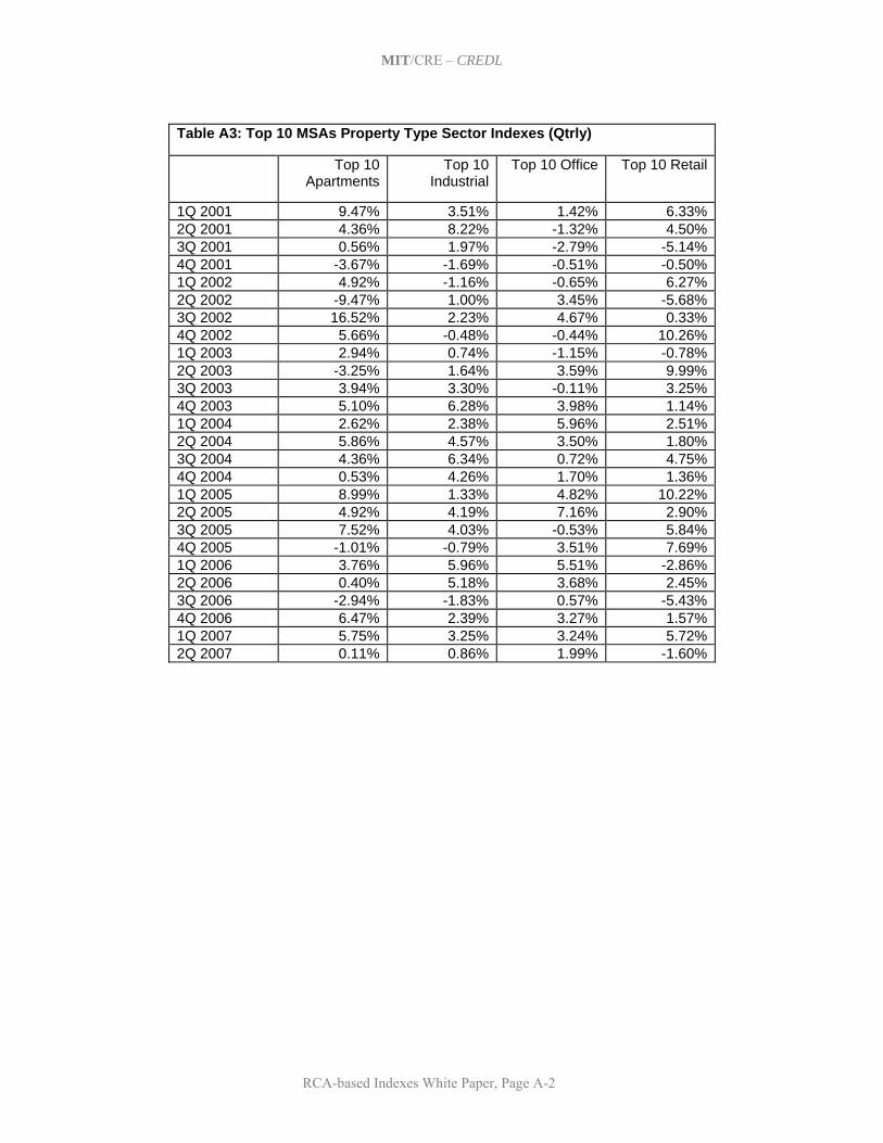
MIT/CRE – CREDL


Table A3: Top 10 MSAs Property Type Sector Indexes (Qtrly)

Top 10 Apartments

Top 10 Industrial

Top 10 Office Top 10 Retail

1Q 2001 9.47% 3.51% 1.42% 6.33% 2Q 2001 4.36% 8.22% -1.32% 4.50% 3Q 2001 0.56% 1.97% -2.79% -5.14% 4Q 2001 -3.67% -1.69% -0.51% -0.50% 1Q 2002 4.92% -1.16% -0.65% 6.27% 2Q 2002 -9.47% 1.00% 3.45% -5.68% 3Q 2002 16.52% 2.23% 4.67% 0.33% 4Q 2002 5.66% -0.48% -0.44% 10.26% 1Q 2003 2.94% 0.74% -1.15% -0.78% 2Q 2003 -3.25% 1.64% 3.59% 9.99% 3Q 2003 3.94% 3.30% -0.11% 3.25% 4Q 2003 5.10% 6.28% 3.98% 1.14% 1Q 2004 2.62% 2.38% 5.96% 2.51% 2Q 2004 5.86% 4.57% 3.50% 1.80% 3Q 2004 4.36% 6.34% 0.72% 4.75% 4Q 2004 0.53% 4.26% 1.70% 1.36% 1Q 2005 8.99% 1.33% 4.82% 10.22% 2Q 2005 4.92% 4.19% 7.16% 2.90% 3Q 2005 7.52% 4.03% -0.53% 5.84% 4Q 2005 -1.01% -0.79% 3.51% 7.69% 1Q 2006 3.76% 5.96% 5.51% -2.86% 2Q 2006 0.40% 5.18% 3.68% 2.45% 3Q 2006 -2.94% -1.83% 0.57% -5.43% 4Q 2006 6.47% 2.39% 3.27% 1.57% 1Q 2007 5.75% 3.25% 3.24% 5.72% 2Q 2007 0.11% 0.86% 1.99% -1.60%

MIT/CRE – CREDL


Table A4: West Regional Property Type Sector Indexes (Qtrly)

West Apartments

West Industrial

West Office West Retail

1Q 2001 0.13% 5.34% 1.52% 4.95% 2Q 2001 4.96% 4.27% -1.86% 1.57% 3Q 2001 2.53% -0.41% -8.79% -1.70% 4Q 2001 -2.36% -2.47% 1.78% 0.85% 1Q 2002 -2.74% -2.77% -6.37% 2.48% 2Q 2002 -0.90% -0.90% 10.31% 0.68% 3Q 2002 9.13% 1.64% -6.64% 4.37% 4Q 2002 7.55% 3.16% -3.16% 1.22% 1Q 2003 0.71% -1.10% 5.39% 1.71% 2Q 2003 -2.44% 1.18% 3.28% 4.09% 3Q 2003 7.26% 0.58% 9.14% 3.63% 4Q 2003 1.68% 7.95% 5.40% 4.75% 1Q 2004 3.34% 0.19% -2.50% 5.40% 2Q 2004 4.80% 4.84% 0.13% 3.09% 3Q 2004 4.29% 5.89% 13.57% 3.12% 4Q 2004 3.62% 6.11% 0.78% 4.45% 1Q 2005 4.26% 0.43% -2.28% 2.59% 2Q 2005 2.06% 3.62% 5.33% 6.03% 3Q 2005 5.18% 7.83% 1.61% 2.50% 4Q 2005 1.79% 1.28% 7.48% 4.28% 1Q 2006 2.67% 6.18% 10.01% 4.33% 2Q 2006 -2.18% 0.28% 1.82% 3.02% 3Q 2006 1.25% -2.50% -5.36% -0.57% 4Q 2006 7.75% 0.81% 5.52% -3.21% 1Q 2007 3.37% 5.15% 2.76% 3.20% 2Q 2007 1.99% 1.37% 6.37% 0.13%

MIT/CRE – CREDL


Table A5: East Region Indexes (Annual) Calendar Year Indexes Returns (CY): Yr Ending Dec:

East Aptment

East Industrial

East Office

East Retail

2001 10.02% 2.06% 2.35% 9.44%2002 15.64% 6.75% 9.13% 17.50%2003 11.71% 12.43% 6.34% 17.18%2004 26.51% 24.95% 13.67% 12.88%2005 18.19% 6.05% 12.46% 18.10%2006 1.31% 8.43% 15.97% 5.33%

Year Ending March Indexes Returns (FYM): Yr Ending March:

East Aptment

East Industrial

East Office

East Retail

2002 16.03% 1.26% 5.57% 7.55%2003 10.21% 5.20% 6.67% 13.43%2004 10.67% 16.23% 6.36% 19.20%2005 33.86% 26.71% 16.09% 16.13%2006 7.38% 0.68% 11.69% 15.58%2007 4.30% 10.28% 14.08% 3.18%

Year Ending June Indexes Returns (FYJ): Yr Ending June:

East Aptment

East Industrial

East Office

East Retail

2002 14.42% 5.20% 2.99% 19.04%2003 12.99% 3.90% 7.90% 5.01%2004 10.20% 14.63% 8.81% 20.51%2005 35.39% 26.89% 16.21% 20.60%2006 -1.43% 3.10% 9.50% 3.69%2007 7.28% 7.07% 15.13% 7.33%

Year Ending September Indexes Returns(FYS): Yr Ending Sept:

East Aptment

East Industrial

East Office

East Retail

2002 11.26% 6.60% 10.23% 14.08%2003 17.66% 6.60% 5.80% 11.48%2004 17.81% 22.81% 9.85% 19.23%2005 24.83% 15.74% 15.25% 19.18%2006 -0.12% 4.30% 12.98% 4.11%

MIT/CRE – CREDL


Table A6: South Region Indexes (Annual) Calendar Year Indexes Returns (CY): Yr Ending Dec:

South Aptment

South Industrial

South Office

South Retail

2001 3.81% 2.28% 2.07% 6.94%2002 5.42% 4.45% 2.30% 9.39%2003 6.64% 2.99% 14.54% 9.33%2004 21.32% 24.88% 9.07% 18.53%2005 28.15% 14.11% 20.58% 13.00%2006 -8.75% 16.05% 6.03% 5.51%

Year Ending March Indexes Returns (FYM): Yr Ending March:

South Aptment

South Industrial

South Office

South Retail

2002 3.01% 10.08% 5.11% 10.07%2003 6.20% 1.09% 2.64% 6.11%2004 6.93% 6.36% 10.98% 9.81%2005 31.15% 25.26% 17.83% 24.65%2006 13.81% 12.12% 17.42% 8.60%2007 -7.99% 13.00% 0.06% 5.52%

Year Ending June Indexes Returns (FYJ): Yr Ending June:

South Aptment

South Industrial

South Office

South Retail

2002 2.69% 8.65% 11.40% 8.80%2003 1.16% 1.40% 6.98% 2.56%2004 10.67% 7.67% 2.60% 15.97%2005 40.47% 23.85% 22.59% 21.08%2006 -2.21% 14.57% 18.02% 9.83%2007 2.31% 11.47% -0.90% 5.40%

Year Ending September Indexes Returns(FYS): Yr Ending Sept:

South Aptment

South Industrial

South Office

South Retail

2002 8.67% 6.24% 8.01% 7.27%2003 5.10% 2.93% 12.04% 0.93%2004 9.16% 16.39% 2.82% 23.28%2005 40.16% 18.32% 22.76% 14.38%2006 -8.79% 17.75% 14.54% 11.36%

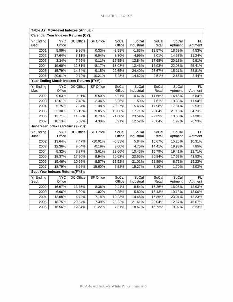
MIT/CRE – CREDL


Table A7: MSA-level Indexes (Annual) Calendar Year Indexes Returns (CY): Yr Ending Dec:

NYC Office

DC Office SF Office SoCal Office

SoCal Industrial

SoCal Retail

SoCal Aptment

FL Aptment

2001 5.59% 9.96% 0.33% -2.58% -1.83% 13.57% 18.69% 4.53% 2002 17.64% 8.11% -6.04% 3.36% 4.99% 8.01% 14.53% 11.24% 2003 3.34% 7.99% 0.11% 16.55% 12.84% 17.68% 20.18% 9.91% 2004 19.60% 12.31% 8.17% 18.03% 13.46% 16.93% 22.03% 25.41% 2005 15.79% 14.34% 9.15% 22.65% 24.40% 25.67% 15.21% 38.81% 2006 20.01% 9.72% 10.21% 6.28% 14.62% 2.51% 2.56% -2.44%

Year Ending March Indexes Returns (FYM): Yr Ending Mar:

NYC Office


SoCal Industrial

SoCal Retail

SoCal Aptment

FL Aptment

2002 9.63% 9.01% -5.50% -5.21% 0.67% 14.56% 16.48% 5.84% 2003 12.61% 7.48% -2.34% 5.26% 1.59% 7.61% 19.33% 11.94% 2004 5.75% 7.34% 1.38% 23.27% 15.48% 17.98% 17.84% 9.53% 2005 22.30% 16.19% 9.85% 15.06% 17.71% 20.84% 21.18% 34.73% 2006 13.71% 11.32% 8.79% 21.60% 23.54% 22.39% 10.80% 27.30% 2007 18.13% 5.52% 4.30% 5.91% 12.52% -3.84% 1.97% -6.93%

June Year Indexes Returns (FYJ): Yr Ending June:

NYC Office


SoCal Industrial

SoCal Retail

SoCal Aptment

FL Aptment

2002 13.64% 7.47% -10.01% -0.33% 5.84% 16.67% 15.26% 10.31% 2003 12.36% 8.04% -0.19% 3.60% 4.75% 14.41% 19.93% 7.85% 2004 8.32% 8.27% 3.61% 22.66% 10.43% 15.79% 19.41% 12.71% 2005 18.37% 17.90% 8.94% 20.62% 22.65% 20.84% 17.67% 43.83% 2006 15.46% 10.69% 8.57% 13.52% 21.01% 21.89% 8.71% 15.23% 2007 18.79% 5.26% 15.60% 6.52% 15.27% 7.10% 1.70% -2.93%

Sept Year Indexes Returns(FYS): Yr Ending Sept:

NYC Office


SoCal Industrial

SoCal Retail

SoCal Aptment

FL Aptment

2002 16.97% 13.75% -8.36% 2.41% 8.54% 15.26% 16.08% 12.93% 2003 6.96% 5.90% -1.02% 9.25% 5.80% 15.43% 19.18% 13.06% 2004 12.08% 6.72% 7.14% 19.23% 14.48% 16.85% 23.04% 12.23% 2005 18.75% 20.54% 7.39% 25.22% 21.61% 20.04% 12.67% 46.67% 2006 16.56% 12.84% 11.22% 7.31% 18.67% 16.72% 9.02% 8.23%

MIT/CRE – CREDL

RCA-based Indexes White Paper, Page B-1

Appendix B:

Equilibrium Pricing of Real Estate Index Return Swaps At the commencement of any new derivatives market, it is important for the market participants to have a basic understanding of the equilibrium pricing principles for the product in question. While the investment industry is amply familiar with derivative products of a great variety, and the real estate industry is very familiar with property asset markets, there may be a gap in familiarity with real estate index derivatives. While derivatives traders are familiar with many types of derivatives, they are not yet familiar with real estate indexes. And while real estate investment professionals are familiar with real estate markets and some types of real estate indexes, they are not familiar with derivatives markets. The result may be a gap in familiarity with basic pricing principles applicable to real estate index return swaps. The knowledge on both sides needs to be integrated. This Appendix aims to help fill this gap by presenting some of the basic pricing fundamentals for real estate price index capital return swaps.* B.1 Basic Mechanics of Index Return Swaps Consider the major type of real estate index return swap that has been vetted so far, the likely type of derivative that would be initially traded on the Moodys/REAL Indexes described in this paper. The index return swaps being considered are essentially futures contracts, in which no cash changes hands up front when the trade is agreed. Instead, a “notional” amount of the trade is agreed, and then the contract is settled periodically based on contemporary index returns, typically at the time of each subsequent index return report, through the time of maturity of the contract. For example, suppose Ms Long and Mr Short agree on a 2-year contract to swap the Moodys/REAL National Monthly Index returns for a fixed amount, based on a notional trade of $100 million. Structurally, this is like a traditional interest rate swap where, for example, one party swaps a floating interest rate for a fixed rate. In such swaps the payments each period reflect a “floating leg” (the variable interest rate) and a “fixed leg” (the fixed interest rate). In the case of the real estate index swap, the “floating leg” would be based on the real estate index return, and we can think of the amount agreed in the “fixed leg” as being the price of the contract. As the real estate index is only a price change index, not a total return index, the floating leg reflects only something akin to an investment capital return. Considering the amount of investment risk in the real estate index, this could well result in a negative fixed leg amount, that is, the short party may pay the long party a fixed component as well as whatever the index return happens to be.

* See also D.Geltner & J.Fisher, “Pricing and Index Considerations in Commercial Real Estate Derivatives”, Journal of Portfolio Management, Real Estate Special Issue, 2007.

MIT/CRE – CREDL


For example, let’s say that Mr Short and Ms Long agree on a fixed leg (price of the long position) of negative 10 basis-points. What happens then? No cash changes hands up front. After the first month, suppose the index return is reported to be positive 100 basis-points. Then Mr Short owes Ms Long 100 bps on the “floating leg” plus another 10 bps on the fixed leg (because the fixed leg is negative). Thus, Mr Short owes Ms Long $1,100,000, or 1.1% of the $100 million notional amount of the swap. The two parties settle up for the first month, leaving the notional balance constant at $100 million. Now suppose the following month the index return comes in at negative 75 bps. Then Ms Long owes Mr Short $650,000, consisting of $750,000 for the negative index return on the floating leg, less the $100,000 (as always) on the fixed leg. The monthly settling of the return swap continues for two years, until the contract expires. The above example also ignores transactions costs and/or any “bid/ask spread”. Such a spread or fees would in practice be necessary to support the transaction facilitators in the middle between the two parties. Derivatives markets require facilitators to get the two trading parties together, as well as administrators and performance guarantors, the costs of which must be paid by the traders. For example, Mr Short might agree to a fixed leg of –15 bps while Ms Long would agree to a fixed leg of –5 bps. The 10 bps/month in between would support the necessary trading facilitators. The implied 120 bps/year transaction costs (across both parties, or 60 bps/year to each party) might be worth it to the trading parties because, for example, Ms Long saves the transaction and management costs and fees of direct property investment, and Mr Short obtains property market value insurance or “hedging” benefits that cannot be otherwise obtained. B.2 Fundamentals of Pricing the Swap Contract: Arbitrage Analysis How would a fair price for the index swap be arrived at in the marketplace? For example, where might the negative 10 bps/month fixed leg amount described in our previous example have come from? In this section, we will consider such pricing using the classical approach of financial economics, arbitrage analysis. This is the approach by which the well-known “Futures Spot Parity Theorem” is traditionally developed (e.g., in typical MBA finance textbooks). Indeed, we shall derive a pricing result for real estate index swaps that is completely consistent with this famous theorem. Later, in Section B.3, we will consider the same pricing problem from an alternative, equilibrium perspective, that does not assume arbitrage. In all of this analysis, we will ignore any market frictions or imperfections, so as to derive the basic pricing results. (You can think of the price result here as the mid-point in the bid/ask spread described previously.) To perform the arbitrage analysis we assume that it is possible to directly trade the underlying index in any fractional amount, both long and short, by trading the properties that are tracked by the index. This of course is not literally possible in the case of the real estate index, but we will relax this assumption in Section B.3, so just be patient! For now, let’s make like economists and assume the existence of perfect and complete markets…

MIT/CRE – CREDL


Let’s go back to our example of Ms Long and Mr Short trading their $100 million notional amount. Only now (to simplify the illustration) let’s assume they are trading an annual frequency index. Suppose further that the riskfree interest rate is a constant 4% per year over the next two years (this could in fact be locked in using bond derivatives), and let’s further assume that the real estate tracked by the index provides a cash yield of 5% per year, which we will assume is constant and riskless.* Let’s represent by the letter F the price of the swap as a fraction of the notional amount (the fixed leg that must be paid by the long position in return for receiving the index return). The question is, what should be the value of F ? Consider the following arbitrage trading strategy for Ms Long. She could:

1. Buy directly $100 million worth of the underlying property portfolio whose price is tracked by the index. This would cost her $100 million up front, but then she would obtain the total return from those properties each year she held the portfolio, including both the 5% cash yield plus any price change that the portfolio experiences each year (the capital return tracked by the index, which could be either positive or negative in any given year, and is uncertain in advance).

2. Sell (or buy) each year that she owns the portfolio an amount of property so as to

realize in cash flow the price change of the portfolio each year (the capital return tracked by the index), so as to keep her property portfolio value balance constant at the original $100 million amount. She would sell when the price change is positive, buy when the price change is negative.

3. Sell the entire property portfolio at the end of two years, realizing $100 million at

that time (since she has kept the value balance constant by her actions under Step 2 above).

4. Issue up front a one-year maturity zero-coupon bond with a par value equal to F +

500 bps (the real estate yield) times the notional amount of $100 million. Let’s assume that Ms Long has taken out a letter of credit or otherwise guaranteed her

* While not strictly true, this is a good working assumption. In fact, the NPI annual cash yield (income return component based on the equal-weighed cash flow based version of the NCREIF Property Index) has exhibited annual volatility of only 1% during the history of the NPI from 1978 through 2005. This is much less than the annual volatility of U.S. Treasury Bills (which was 3.2% during the same period, according to Ibbotson Assoc.), which are often taken as a proxy for a “riskfree” asset. The volatility in the transactions price based MIT TBI income return component during its history since 1984 has been similar, at 0.9%/year, far less than T-Bill volatility during that period. As real estate annual net income is typically less than one-tenth asset values, the present value perpetuity formula (aka the “Gordon Growth Model”) implies that a one point change in income return will correspond to more than a 10-point change in annual capital return. Thus, basic mathematics forces the capital return volatility to dominate within the total return volatility. This is the fundamental reason why it is not necessary to trade a total return swap; the capital return swap alone captures virtually all of the relevant volatility. The typical rate of real estate cash yield can be observed in the real estate market, for example, as the prevailing “cap rates” (net operating income divided by property price) less the typical annual expenditure on routine capital improvements for the upkeep of property (typically 100 to 200 bps per year). Cap rates are typically reported by real estate market watchers, including RCA. In 2006 RCA reported cap rates typically in the 6% to 7% range, suggesting annual cash yields around 5%.

MIT/CRE – CREDL


credit so that she can issue this zero-coupon bond at the riskfree interest rate of 4%. Then (ignoring her cost of guaranteeing her credit), this bond issuance (borrowing transaction) will net her up front an amount equal to (F + 0.05)*$100 million / (1.04). However, at the end of Year 1 she will have to pay back the amount (F + 0.05)*$100 million.

5. Similarly to in Step 4 above, issue up front a riskless zero-coupon bond (borrow)

again, only now for two years, and with a par value of F plus the 5% yield times the $100 million notional trade amount, plus now also the notional value itself, an additional $100 million. This will net her up front an amount equal to (F + 1.05)*$100 million / (1.04)2. However, at the end of Year 2 she will have to pay back the amount (F + 0.05)*$100 million plus the $100 million principal.

The cash flow impacts of all of these actions, both up front and in each of the next two years (through the unwinding of the entire arbitrage operation) are summarized in the table below, with gt representing the real estate price change percent in any year t, the return tracked by the real estate index.* Notice in the bottom row of the table, which sums all the cash flows within each period, that while the real estate price changes during the next two years are risky and their values are unknown, the offsetting borrowing operations done by Ms Long eliminate all risk in the overall arbitrage operation, which will provide zero net cash flow in each of the next two years, for certain.

Cash Flow at t Cash Flow at t+1 Cash Flow at t+2 Buy the underlying property portfolio tracked by the index, then sell in 2 yrs.

- $100M (gt+1 + .05) *$100M (gt+2 + .05) *$100M + $100M

Short the RCA-based index return swap @ price F for 2 yrs.

0 (F - gt+1) *$100M (F - gt+2) *$100M

Issue riskless zero-coupon bond (borrow) for 1 year, amt F + 5% of notional

(F + .05) *$100M / 1.04 - (F + .05) *$100M

Issue riskless zero-coupon bond (borrow) for 2 yrs, amt F + 105% of notional

(F + 1.05) *$100M / (1.04)2 - (F + .05) *$100M - $100M

Total (F + .05) *$100M / 1.04 + (F + 1.05) *$100M / (1.04)2 - $100M

0 0

* Note that gt is the capital gain component of the total investment return: gt equals the total investment return less the cash yield component described previously, where the cash yield is net of capital improvement expenditures made to keep up the property.

MIT/CRE – CREDL


If the overall arbitrage operation nets zero cash flow in all future periods for certain, then any positive net cash flow it achieves up front will be riskless profits (“arbitrage profits”). In fact, any negative net cash flow achieved up front would also equate to the ability to earn riskless (arbitrage) profits as well, because in our world of “perfect markets” we could just reverse all of the above-described transactions (e.g., turn Ms Long into Mr Short and sell short the underlying property portfolio instead of purchasing it, and then going long in the index swap, lending rather than borrowing the other amounts). Thus, any net cash flow value up front other than zero would allow for riskless arbitrage profits. Assuming trading in the market would tend to drive such profits to zero, we have the arbitrage-based equilibrium pricing condition established by setting the up front net cash flow amount equal to zero. This gives the following pricing equation, which is solved below for the values in our example.

( ) ( )

01.05.04.

04.05.

04.111

04.111

100$04.1

05.04.1

05.100$04.111

0100$04.1

100$04.1

100$05.04.1

100$05.

22

22

22

−=−=

+⎟⎠⎞

⎜⎝⎛ −=−

⎟⎠⎞

⎜⎝⎛ +

++

=⎟⎠⎞

⎜⎝⎛ −

=−++

++

F

F

MFFM

MMMFMF

Thus, we see that the implied equilibrium price in our example is a fixed leg rate of negative 100 bps per annum. This is approximately the same magnitude as the negative 10 bps per month as we used in the monthly frequency example in Section B.1. Then above result is generalizable to periodically settled contracts of any length maturity. The general equilibrium (arbitrage-based) price result is: F = rf – y (B1) where rf is the riskfree interest rate and y is the real estate cash yield rate (or income return component, the expected total return less the expected price growth rate tracked by the real estate index). But this result has been derived using the assumption of perfect and complete markets, which we know do not exist in real estate. The types of trades described in the arbitrage operation in this section could not actually take place. What are the pricing implications of a more realistic approach?...

MIT/CRE – CREDL


B.3 Fundamentals of Pricing the Swap Contract: Equilibrium Analysis A more realistic analysis of the equilibrium price of the swap contract can be obtained if we consider the perspectives of “covered” traders on both sides of the swap. A “covered” trader is one who holds assets that notionally back his or her obligations under the swap contract. Unlike the arbitrage scenario, in this case we will not require that the coverage be perfect. The backing assets may not be perfectly correlated with the swap obligations, but they will be related to the opposite side of the swap position in a manner that reflects the actual underlying assets in the real world. In particular, we will assume that the party taking the long position in the swap will hold riskless bonds in an amount equal to the notional value of the swap trade. And we will assume that the party taking the short position in the swap will hold real estate assets similar to those tracked by the index and in a value equal to the notional amount of the swap trade. Thus, both parties are somewhat hedged in their swap obligations. In this model, even though the swap contract itself takes no up front cash investment, the two parties in the swap trade are effectively making up front investments of the notional amount of the trade, in the sense that they are incurring the opportunity cost of holding the covering positions. In fact, in the real world, there must be, somewhere, bond holdings sufficient to back the long position fixed leg obligations, and real property holdings sufficient to back the short position floating leg obligations, even if these holdings are not held directly by the swap trading participants. The ability to trade within and across the bond and property markets insures that this covered trader perspective is relevant for understanding equilibrium pricing, even when the actual traders themselves are not covered and therefore the backing assets are not directly involved.

From this perspective, both sides in the swap trade need to get a fair ex ante return expectation as if they were making an actual up front investment of the notional amount of the trade. To see the implications for equilibrium pricing, let us establish the following notation:

• EL[gRCA] & ES[gRCA] = Ms Long’s and Mr Short’s expectations (respectively) of the underlying real estate index average capital (price change) return over the swap contract horizon.

• E[RPRCA] = The market’s required expected (equilibrium) total return risk premium (excess over the riskfree return) to investments with risk like that of the underlying real estate index, assumed also the same as that for the real estate portfolio covering Mr Short’s position.

• ES[yS] = Mr Short’s expectation of the income return component of his covering real estate portfolio, assumed effectively constant and riskless.

• ES[rS] = ES[yS] + ES[gS] = Mr Short’s expected total return on his covering real estate portfolio over the contract horizon.

• rf = The riskfree interest rate over the contract horizon.*

* We’ll continue to simplify away from the differing credit ratings that different traders might have by assuming that all parties pay on the side as necessary to guarantee their performance under the swap contract.

MIT/CRE – CREDL


• F = The fixed leg rate paid by the long party to the short party, expressed as a fraction of the notional amount of the trade (the price of the swap contract).

From this perspective, for every dollar of notional amount that Ms Long trades in the swap contract, she will automatically receive rf per year in riskless interest from her covering bond holdings. She will also receive gRCA,t each period t from the swap long position, and she will have to pay out F in her obligation under that position. The risk that she faces is that of the risk in the real estate index, and so she requires an expected total return sufficient to compensate for such risk: rf + E[RPRCA]. Thus, Ms Long’s expected return requirement is given by the following inequality:*

EL[gRCA] – F + rf ≥ rf + E[RPRCA] (B2a) On the other side, Mr Short has essentially swapped the risky capital return component of his covering property holdings’ total return for the riskless fixed leg, F. This makes his position virtually riskless, which should make him satisfied with an expected return of rf , the riskfree rate. More precisely, for every dollar of the notional amount of the swap trade, Mr Short takes in his covering portfolio’s total return each period, rS,t , plus F in the fixed leg paid by Ms Long, and he pays out only the index capital return, gRCA,t . Thus, Mr Short’s requirement is that he must face an expected return that satisfies the following inequality:

F – ES[gRCA] + ES[rS] ≥ rf (B2b) These two inequalities must both be satisfied, and there is only one variable to manipulate to do this, the swap price variable: F. Depending on the parties’ expectations, there may not always be a solution, and if there isn’t, then no trade would be possible between these two parties. But trading should be possible depending on the parties’ expectations. The general condition that F must satisfy is: rf – ES[rS] + ES[gRCA] ≤ F ≤ EL[gRCA] – E[RPRCA] (B3)

Now suppose first that both parties share the same expectations, that all relevant returns will be identical to those of the underlying real estate index:

ES[rS] = ES[rRCA] = EL[rRCA] = E[rRCA] = rf + E[RPRCA], and

ES[gRCA] = EL[gRCA] = E[gRCA].

Then (B3) reduces to:

* We continue to ignore bid/ask spread or fees, but each party’s return expectation would actually have to be net of any such spread or fee. The price, F, that we are therefore aiming at here should be thought of for now as the mid-point in the bid/ask spread.

MIT/CRE – CREDL


rf – E[rRCA] + E[gRCA] ≤ F ≤ E[gRCA] – E[RPRCA] rf – (rf + E[RPRCA]) + E[gRCA] ≤ F ≤ E[gRCA] – E[RPRCA] –E[RPRCA] + E[gRCA] ≤ F ≤ E[gRCA] – E[RPRCA]

F = E[gRCA] – E[RPRCA] (B4) Thus, the equilibrium analysis gives the pricing rule that the fixed leg rate should equal the expected return on the underlying real estate price index less the market’s required equilibrium total return risk premium on such real estate. How does this pricing rule compare to the arbitrage-based pricing rule that says that the fixed leg rate should be the riskfree rate minus the expected cash yield on the underlying real estate? If the real estate index reflects the equilibrium pricing in the real estate market, then the two rules are equivalent. To see this, note that in equilibrium the expected total return on the real estate underlying the price index is the riskfree rate plus the equilibrium expected risk premium:

E[rRCA] = rf + E[RPRCA] Thus: E[RPRCA] = E[rRCA] – rf . Substituting this into (B4) we obtain:

F = E[gRCA] – (E[rRCA] – rf ) = rf + E[gRCA] – E[rRCA] But by definition: E[rRCA] = E[gRCA] + E[yRCA] . Therefore: E[gRCA] – E[rRCA] = -E[yRCA]. Therefore, we see that the above expression (B4) is equivalent to the arbitrage pricing result in (B1): F = E[gRCA] – E[RPRCA] = rf – E[yRCA] While this pricing rule will not always give a negative value for F, it more often than not will. For example, in the NCREIF Index (which explicitly tracks both components of the total return), the historical average annual total return during the complete 20-year market cycle from 1984 through 2003 was 7.7%. This consisted of 6.1% cash yield (y) plus 1.6% capital growth (g).* During this 1984-2003 period the riskfree interest rate, rf as proxied by T-bills, averaged 5.4%, implying that RP was about 2.3%. Thus, during 1984-2003 on average the market provided a 7.7% total return (including a 2.3% risk premium) to compensate institutional real estate investors for the amount of risk in institutionally-held real estate. Taking these as equilibrium values, the above formula for the fixed leg price of the capital return swap would have been:

F = 1.6% – 2.3% = 5.4% – 6.1% = –0.7% That is, the fixed leg would have been negative 70 bps/year, or about negative 6 bps/month. * These figures are based on the equal-weighted, cash flow based version of the NCREIF Property Index (NPI). This is the version of the NPI that is most directly comparable to the RCA Index.

MIT/CRE – CREDL


B.4 A Caveat for Disequilibrium: Difficulties with Appraisal-Based Indexes The analysis in Sections B.2 and B.3 provide a pretty robust underpinning for understanding the equilibrium pricing of the capital return swap contract when the underlying real estate index reflects the equilibrium pricing of the properties within the property market. However, this will not always be the case, particularly if the real estate index on which the swap contract is based is an appraisal-based index, such as the NPI, rather than a fully up-to-date contemporary transaction price based index such as the Moodys/REAL Index. As noted in Section 1 of this paper, the appraisals on which the NCREIF Property Index is based tend to have a temporal lag bias (consistent with property professional appraisal procedures), and most of the NCREIF properties are not reappraised every quarter, causing an additional “stale appraisal” effect in the index. The result is that the NPI exhibits a temporal lag bias and very strong inertia in its capital returns. Whenever the property market has been moving strongly in one direction or is at a turning point or inflexion point in the market price cycle, the NPI tends not to reflect equilibrium prices in the property market. More precisely and to the point, the realistic expected return going forward in the NPI in such circumstances tends to differ from the property market’s realistic expected return going forward based on current actual transaction prices in the property market. In these circumstances, the arbitrage pricing rule (B1): F = rf – E[yNPI] , does NOT apply as a fair equilibrium price for a swap contract based on the NPI. However, the more general equilibrium pricing rule (B4): F = E[gNPI] – E[RPNPI] , still holds, with the interpretation that E[gNPI] should reflect the expected appreciation in the Index (including the lag effect or inertia), while E[RPNPI] should reflect the investment market’s realistic equilibrium risk premium requirement for the NPI.* In any case, such theoretical pricing challenges should be of less concern in a well constructed, contemporaneous transactions price based index that avoids temporal aggregation and temporal lag bias, and the Moodys/REAL Indexes have been designed with this in mind. It should nevertheless be noted that, while the indexes may not lag the property market, it is possible for the underlying property market to have some sluggishness or momentum even in its equilibrium. That is, prices can be persistent in the real property market. It is generally believed that private search markets trading whole assets will often not be as informationally efficient as public securities exchanges. To the extent the property market has inertia or predictability in its returns, this should be reflected contemporaneously in a well-constructed transactions price index. In this case, the derivatives market will try to incorporate any resulting property market predictability into the pricing of the derivatives, enabling the derivatives market pricing to help inform the

* This risk premium may differ from (probably be less than) the risk premium required by the underlying property investments, because the appraisal smoothing and lagging in the NPI may give that index less risk than the average risk in the underlying property market. In other words, in classical “CAPM” terminology, the “beta” of the NPI may be less than the average beta of the properties that compose the NPI.

MIT/CRE – CREDL


property market where prices may be headed that the property market itself has some inertia. B.5 Arbitrage Derivation of Swap Price with a Lagged Index or Sluggish Market To provide some additional insight on the pricing of real estate index swaps even when the index is lagged or the property market has momentum, this section presents an arbitrage model of the equilibrium price of a swap on an index that is lagged and smoothed, or, alternatively interpreted, the index is not lagged but the property market has momentum. Assume the following total return generating process for the underlying property market tracked by the index, or, in the alternative interpretation, for the news innovations (and drift) underlying the lagged market:

.0]~[:,][

:,~

==+=

tPPt

tPPt

EandrrEwhererr

σσ

(1)

E[rPt] = rP is the expected total return to the property market, a deterministic constant, and STD[ tσ~ ] is the volatility of the property market. The realizations of tσ~ are random innovations with a mean of zero (white noise). Thus, if we interpret (1) as the property market, then that market is behaving as if it were informationally efficient, with no momentum in its prices. Alternatively, we can interpret (1) as reflecting contemporaneous news innovations underlying a sluggish market (what the property market returns would be if the market were informationally efficient). In this latter interpretation we assume that the index is a faithful contemporaneous representation of the actual property market, but that market has momentum, reflecting its underlying innovations only gradually and with some smoothing. With the above in mind, assume the following total return generating process for the real estate index (or in the alternative interpretation for the property market itself where that market is sluggish). This process is general enough to capture the essential features of a lagged index, such as an appraisal-based index, or of a sluggish market, for purposes of understanding the basics of swap pricing:

1:,~

≥++= HwheremH

rr tPSt

σ (2)

E[rSt] = rP + m is the expected return to the index (or the sluggish market), a deterministic constant, and STD[ tσ~ ]/H is the volatility of the index (or the sluggish market). H may be interpreted as the “hedge ratio” of the index, the amount of notional value of the index that must be traded in order to completely hedge one dollar’s worth of property market exposure. Alternatively, H is the hedge ratio of the tradable market compared to the innovations underlying that market. The index (or sluggish market) volatility is thus reduced below that of the efficient property market (or the innovations underlying the market) by the factor 1/H. The term m is the “momentum” in the index (or the market), reflecting autocorrelation in returns, caused by the lag in the index (or market). The magnitude and sign of m will depend on the strength and direction in which property market prices (or innovations) have recently been moving. When the property market has

MIT/CRE – CREDL


been increasing in value greater than its long-run equilibrium rate, m will be positive (and vice versa). In a “perfect” index that exactly tracks an efficient underlying property market, H = 1, and m = 0. Thus, H > 1 models the volatility-damping effect of index lag or of market sluggishness, while m <> 0 models the momentum or predictability effect of such lag or sluggishness. We ignore (as in any arbitrage price derivation) any “basis risk” between the index and the underlying property market (or in the alternative interpretation, between the market and its underlying innovations). From this point on in this section we will present the model as though it applies to a lagged index tracking an informationally efficient market. The alternative interpretation of an up-to-date index tracking a sluggish market would proceed in a parallel and analogous manner, substituting “market” for “index”, and substituting “underlying news innovations” (or what the market returns would be if the market were efficient) for “market”. With this in mind, note that the above model implies that the equilibrium ex ante total return risk premium in the index is (1/H ) times the equilibrium risk premium in the underlying property market: RPS = (rS – rf ) = (rP – rf )/H = RPP/H (3) where rS is the equilibrium (long-run: m = 0) expected total return in the index: EE[rS]. The actual expected return in the index differs from this equilibrium expectation not only due to m<>0 in the short run, but also because rP > rS to the extent the index presents reduced risk compared to the underlying property market. This difference is possible because the index itself is not directly traded, and hence need not be in equilibrium. To perform the arbitrage analysis we assume that it is possible to directly trade the underlying property market in any fractional amount, both long and short, as well as the index tracking the market via the swap derivative. Of course, if it were really possible to directly and frictionlessly trade the underlying property market, the index would no doubt not be lagged and smoothed as represented here. But the model examined here is designed to elucidate the essential features of equilibrium pricing of the swap contract in the realistic situation where the index may indeed be lagged and smoothed as modeled here. It should also be noted that this model of the index return generating process relative to the underlying property market is even so a simplification, and it will only be a good approximation over short periods of time. But derivative contracts will typically be traded over relatively short horizons. Now consider the construction of an arbitrage or hedge based on an amount V of real estate market value exposure in the underlying property market. This amount of property exposure can be hedged by HV worth of notional value of the swap contract. Consider a two-period swap, and represent the riskfree interest rate as rf. The price of the swap is F, quoted as a fraction of the notional amount of the swap contract traded (the fixed leg that must be paid to the short position by the long position in return for receiving the index return from the short position). The question is, what should be the value of F ?

MIT/CRE – CREDL


Consider the following arbitrage trading strategy to hedge property exposure using the long position in the swap:

6. Sell (short if necessary) V worth of the underlying property market tracked by the index. This will yield V dollars cash up front. This sale will then owe the total return from the property market each period, rPt (will receive cash when rPt is negative). Note that this will keep the balance in the short position constant at V. Payment each period will be (rP + tσ~ )V.

7. Close out the short position in the property market at the end of two periods, paying

the amount V at that time (since the value balance has been kept constant by the actions under Step 1 above).

8. Buy (long) notional amount HV of a two-period total return swap based on an index

that tracks the property market sold short in (1), for price F. This requires zero cash outflow up front, and then receives each period the amount (rP + tσ~ /H + m – F )HV . This swap purchase will hedge the risk in the short position in the property market, offsetting the uncertain component of the return: tσ~ V, leaving the overall long/short position with a (certain) cash flow each future period of: ((H-1)rP + Hm – HF )V, as well as the cash outflow of V in the second period (per Step 2).

9. Sell (borrow) up front a riskless one-period maturity zero-coupon bond with a par

value equal to ((H-1)rP + Hm – HF)V. This will net cash flow up front of ((H-1)rP + Hm – HF)V/(1+rf), in return for the outflow of ((H-1)rP + Hm – HF)V in period 1, which will exactly offset the certain cash flow from the long/short index/property position at that time, leaving period 1 with a net cash flow of zero for certain.

10. Similarly to in Step 4 above, sell up front a riskless zero-coupon bond (borrow)

again, only now for two years, and with a par value of ((H-1)rP + Hm – HF – 1)V. This will net cash flow up front in the amount of: ((H-1)rP + Hm – HF – 1)V/(1+rf)2, in return for the outflow of ((H-1)rP + Hm – HF – 1)V in period 2, which will exactly offset the certain cash flow from the long/short index/property position at that time, leaving period 2 with a net cash flow of zero for certain.

The cash flow impacts of all of these actions, both up front and in each of the next periods (through the unwinding of the entire arbitrage operation) are summarized in the table below. Notice in the bottom row of the table, which sums all the cash flows within each period, that while the real estate price changes during the next two years are risky and their values are unknown, the offsetting borrowing operations eliminate all risk in the overall arbitrage operation, which will provide zero net cash flow in each of the next two years, for certain.

MIT/CRE – CREDL


Cash Flow at t Cash Flow at t+1 Cash Flow at t+2 Sell (short) amount V of the property market tracked by the index, then buy back in 2 periods.

V -V(rP + 1~

+tσ ) -V(1 + rP + 2~

+tσ )

Buy (long) an amount HV of the index total return swap @ price F for 2 periods.

0 HV(rP + 1~

+tσ /H + m – F) HV(rP + 2~

+tσ /H + m – F)

Sell (borrow) riskless zero-coupon bond for 1 period, par value amount: ((H-1)rP + Hm – HF)V.

((H-1)rP + Hm – HF)V/(1+rf)

-((H-1)rP + Hm – HF)V 0

Sell (borrow) riskless zero-coupon bond for 2 periods, par value amount: ((H-1)rP + Hm – HF – 1)V.

((H-1)rP+Hm–HF–1)V/(1+rf)2

0 -((H-1)rP + Hm – HF – 1)V

Total

V + ((H-1)rP + Hm – HF)V/(1+rf) + ((H-1)rP+Hm–HF–1)V/(1+rf)2

0 0

Since the future net cash flow of the position is zero for certain in all future periods, the present value of the position must also be zero to avoid arbitrage. Thus we set the amount in the time t bottom cell equal to zero, and solve for F to find the arbitrage price of the swap:

MIT/CRE – CREDL


where RPP is the equilibrium risk premium in the underlying property market, and RPS is the equilibrium risk premium on the index underlying the swap, and L is the “index lag effect”. In summary, the arbitrage-based price derivation for the swap is: F = rf + L , where: L = (RPP – RPS ) + m (4) If the index is “perfect” (no lag), then H = 1, and m = 0, making L = 0, and the swap price reduces to the riskfree interest rate: F = rf , the classical price from the “Futures-Spot Parity Theorem”. If the index is lagged, then the swap price adds the “lag effect”, L, to this classical result: F = rf + L, where L consists of two components: the difference in the equilibrium risk premia between the property market and the index (RPP – RPS ), and the “momentum” effect in the index: m (the predictable component of the index return reflecting the lag of previous property market price changes not yet reflected in the index). Note that an equivalent way of expressing L is that it is the difference between the actual expected return on the index and the equilibrium expected return on the index, during the life of the derivative contract: L = E[rS] – EE[rS] (5)

( ) ( )( )

( ) ( ) ( )

( ) ( )( )

( )

( ) ( ) mRPRPLwhereLrFmRPRPrF

mHrrrrrFmHrrrF

HrrmHrFrHHmrHFrHHmHFr

rrHHmHF

rVV

r

rHHmHFrr

VVr

rVHFHmrH

rVHFHmrHV

SPfSPf

fPfPffPP

PPfPfPf

f

P

ff

Pfff

f

P

f

P

+−=+=⇒+−+=

+−−−+=⇒+−−=

−++=⇒−++=⇒−−−=

−−−⎟⎟⎠

⎞⎜⎜⎝

⎛

+−=

⎟⎟⎠

⎞⎜⎜⎝

⎛

+−

−−−⎟⎟⎠

⎞⎜⎜⎝

⎛

++

+=

⎟⎟⎠

⎞⎜⎜⎝

⎛

+−

=+

−−+−+

+−+−

+

:,,

/)()(,/)(

//,)1(,)1(

)1(1

111

11

)1(1

11

11

11

01

1)1(1

)1(

22

22

2

MIT/CRE – CREDL

RCA-based Indexes White Paper, Page C-1

Appendix C: A Further Numerical Example of the Repeat-Sales Regression Model

Section 4.1 in the main body of this paper presented a very simple numerical example to demonstrate how the repeat-sales regression model works to enable estimation of the percentage price changes (capital returns) in each individual period of time when the property transactions database consists of properties that are held across multiple periods of time. To keep that example very simple, we posited only two properties and two periods of time, and this necessitated that one of the repeat-sales corresponded to a single period investment holding period (Property #2 was bought and sold at the beginning and end of Period 2). But the ability of the repeat-sales model to derive the individual periodic returns was not dependent on having any such single-period observations in the estimation database. In this Appendix we will present a slightly more complicated numerical example (three properties and three periods instead of just two), which demonstrates this point. In so doing, we will also highlight other key features of the repeat-sales model that are not intuitively obvious, such as how the model can detect a downturn in the market even when all of the individual property investments are producing a positive return over their holding periods, and how no single period’s return estimate is based only on the second-sales occurring in that period alone. In this example, suppose that the true returns in the market are respectively: 0%, +10%, and -5%, in three consecutive periods (say, 2007, 2008, and 2009). Thus, a true price index starting out at 1.00 at the end of 2006 would remain at 1.00 at the end of 2007, jump to 1.10 in 2008, and then fall back to 1.045 in 2009 [as (1.045 – 1.10)/1.10 is -5%]. Now suppose we have three property repeat-sales observations involving altogether at least one sale in each of the three years, with each being consistent with the true returns but in which no one observation can directly reveal any one period’s return because the properties are held across more than one period. Property #1 is bought at the beginning of 2007 for $100,000 and sold after three years at the end of 2009 for $104,500. Property #2 is also bought at the beginning of 2007, but for $200,000 and sold at the end of 2008 for $220,000 (held for two years). Property #3 is bought at the beginning of 2008 for $300,000 and sold at the end of 2009 for $313,500 (also held two years). This is summarized in the table and figure on the following page, where the figure indicates both the true market price index (the solid line) and the capital returns achieved by each of the three investors in these three properties (dashed lines). Defining the RSR model as described in Section 4.1 (only with the minor modification that we will work in log price ratios, defining the dependent variable, “Y”, to be the natural logarithm of the ratio of the second sale price divided by the first), we have the estimation data indicated in the table below. For example, $313,500/$300,000 is 1.045, and the natural log of this value happens to be about 4.4%.

MIT/CRE – CREDL


RSR Estimation Data Y value

= LN(Ps/Pf)

X2007 value

X2008 value

X2009 value Observation # 1 LN(1.045) 1 1 1 Observation # 2 LN(1.10) 1 1 0 Observation # 3 LN(1.045) 0 1 1

Our regression equation can now be expressed as:

Y = a2007(X2007) + a2008(X2008) + a2009(X2009) , And the three simultaneous equations for estimating the regression from the data are:

LN(1.045) = a2007 (1) + a2008 (1) + a2009 (1) (C1) LN(1.100) = a2007 (1) + a2008 (1) + a2009 (0) (C2)

LN(1.045) = a2007 (0) + a2008 (1) + a2009 (1) (C3) Which equates to:

LN(1.045) = a2007 + a2008 + a2009 (C1) LN(1.100) = a2007 + a2008 (C2)

LN(1.045) = a2008 + a2009 (C3)

2007 2008 2009

1.001.00

1.10

1.045Prop # 1Prop # 3

Prop # 2

Numerical Example of Repeat-Sales Regression ModelPrices Observed at Ends of Years:

2006 2007 2008 2009 True Price Index 1.00 1.00 1.10 1.045 True Capital Return 0% 10% -5% Property # 1 $100,000 No Data No Data $104,500 Property # 2 $200,000 No Data $220,000 No Data Property # 3 No Data $300,000 No Data $313,500

MIT/CRE – CREDL


We thus have three linear equations with three unknowns (a2007, a2008, and a2009, representing the true log price ratios in each of the three periods). Such a system can always be solved, and in this case the solution can be found as follows, for example… Use Eq.(C2) to derive: a2008 = LN(1.1) – a2007. The plug this into Eq.(C3) to obtain: a2009 = LN(1.045) – LN(1.1) + a2007. Now plug both of these into Eq.(C1) to obtain:

LN(1.045) = a2007 + [LN(1.1) – a2007] + [LN(1.045) – LN(1.1) + a2007], a2007 = LN(1.045) – LN(1.045),

a2007 = 0. Now plug this result back into Eqs.(C2) and (C3) to obtain: a2008 = LN(1.1), and a2009 = LN(1.045) – LN(1.1). The result that a2007 = 0 simply means that the estimated price index level did not change during 2007. From the definition of logarithms we have 0 = LN(1), and algebraically we can express this as LN(1/1). Similarly, we can expresse a2008 = LN(1.1) as LN(1.1/1). Thus, the implied log price ratios of the price index ending values divided by its beginning values each year are:

For 2007 = a2007 = LN(1/1) For 2008 = a2008 = LN(1.1/1) For 2009 = a2009 = LN(1.045/1.1)

Exponentiating these values, we arrive at the implied straight level price index as of the end of each year as follows:

2006 = 1.000 2007 = 1.000 2008 = 1.100 2009 = 1.045,

with the resulting implied price-change percentages (capital returns): 2007 = 0% 2008 = +10% 2009 = - 5%.

Thus, we see that the repeat-sales model has derived the true capital return in each period, even though no single repeat-sale price change observation corresponded to any one year. The model correctly derived the negative return in 2009, even though none of the repeat-sale observations used in the estimation showed a negative price change in itself. In other words, all of the three investors made a positive resale gain over their holding periods. Note also that the estimation of the returns in each of the three periods was affected by all three of the repeat-sale observations. For example, the estimate of the –5% return in 2009 was determined in part by the +10% return obtained on Property #2, even though that property’s second sale occurred prior to the beginning of 2009. While this is a simple numerical example, the type of result shown here is general. In principle, the repeat-sales model only requires one sales observation per period (either a first or second sale) in order to be able to estimate the true return each period, even though no single repeat-sale pair corresponds to any one period. And the model uses ALL

MIT/CRE – CREDL


observations to estimate EVERY period’s return. Thus, it is not correct to think that the estimated return in the current period is determined solely or in isolation by the second-sale observations in the current period. Of course, as discussed in Section 4.2, in the real world individual transaction prices will be dispersed randomly around the relevant market values, which makes index estimation a statistical process. The existence of more than one observation (hence more than one equation) in each period of time enables such estimation to be optimized in various ways, as described in Section 4.2.

MIT/CRE – CREDL

RCA-based Indexes White Paper, Page D-1

Appendix D: A Method for Deriving Quarterly Indexes from Staggered Annual Indexes for the

Purpose of Supporting Derivatives Trading In Section 5 we presented indexes covering 16 market segments at the annual frequency, with four staggered versions of these indexes each starting one quarter after the other. (We labeled these the CY, FYM, FYJ, and FYS indexes.*) The 16 market segments include all four property sectors in the East and South NCREIF Regions and in our Southern California MSA cluster, plus three office markets in the New York, Washington DC, and San Francisco MSAs, and the apartment sector in our South Florida MSA cluster. It is necessary to produce indexes at the annual frequency in these 16 markets segments because there is insufficient data to produce quarterly indexes directly via the repeat-sales regression method. However, it is possible to produce quarterly indexes for these 16 markets by deriving the quarterly returns implied by the staggered annual indexes. In this appendix we describe a method for doing this, and we will show an example of what the resulting derived quarterly indexes look like. At present, these derived quarterly indexes are not being produced and published by Moodys, but analysis of this technique is continuing at MIT, and it is possible that indexes like these may be produced and published in the future.

As an example of this approach, consider the Retail index of the Southern California MSA cluster (LA region + San Diego). The chart above shows the four staggered annual indexes with the derived quarterly index superimposed on them. Note how the derived quarterly index is generally consistent with the annual returns that span each quarter. However, the quarterly index picks up the changes implied by changes in the staggered annual indexes. * Note that these are not “rolling” annual indexes in the sense that each index presents sequential consecutive annual returns with no overlap between the years as defined within each index. Each index is therefore a series of “independent” annual returns.

Retail: Southern California MSA

0.8

1

1.2

1.4

1.6

1.8

2

2.2

2.4

2.6

2000

Q4

2001

Q1

2001

Q2

2001

Q3

2001

Q4

2002

Q1

2002

Q2

2002

Q3

2002

Q4

2003

Q1

2003

Q2

2003

Q3

2003

Q4

2004

Q1

2004

Q2

2004

Q3

2004

Q4

2005

Q1

2005

Q2

2005

Q3

2005

Q4

2006

Q1

2006

Q2

2006

Q3

2006

Q4

2007

Q1

CY FYM FYJ FYS Derived Qtrly

MIT/CRE – CREDL


For example, while the FYS annual index ending in 2006Q3 was positive, it was less positive than the immediately preceding FYJ annual index ending in 2006Q2. (The FYS ending in 2006Q3 was up 17% but the FYJ ending in 2006Q2 was up 22%.) The resulting derived quarterly index indicated an essentially flat quarterly return in 2006Q3. When the CY2006 annual index (ending in 2006Q4) then came in at a barely positive 2.5%, the derived quarterly index combined that with the +17% return over the four quarters ending in 2006Q3 to indicate a drop of 6.4% during the fourth quarter of 2006. At first it may seem odd that the derived quarterly index can be negative when the annual indexes that span the quarter are all positive. The intuition behind a result such as the above example is that a subsequent annual index could still be increasing as a result of rises during the first 3 quarters of its 12-month time-span, with a drop in the last quarter that does not wipe out all of the previous three quarters’ gains. For example, suppose the following are the true quarterly changes during the past 5 quarters: 06Q1 = +3%, 06Q2 = +3%, 06Q3 = +3%, 06Q4 = +3%, 07Q1 = -4%. Then the CY06 annual index would show +12% (ending 12/31/06), and the FYM07 annual index would show +5% (ending 3/31/07), even though the 07Q1 quarterly return is negative. When the most recent annual index is rising at a lower rate than the next-most-recent annual index, it can (although does not necessarily) indicate that the most recent quarter was negative. The derived quarterly return methodology is designed to discover and quantify such situations as best we can. Simple curve-fitting of the annual indexes introduces considerable smoothing, and will not be able to pick up the kind of turning points we have just described. The derived quarterly index methodology described in this appendix is not perfect. It probably introduces a small amount of additional noise, and it can exaggerate market movements during periods of sustained increasing or decreasing returns (booms or busts). Even if the absolute amount of noise is the same, the signal/noise ratio is less per period in a higher frequency index, making the noise possibly more apparent in a given return report.* Nevertheless, we find that the derived quarterly index methodology described in this appendix performs better than direct quarterly estimation in circumstances where the data is too scarce for good direct quarterly estimation, such as the 16 markets where we produce staggered annual indexes. In the methodology description below, we will layout the derivation of a quarterly index from staggered annual indexes. More generally, the method refers to derivation of an index with independent return reporting periods at frequency “Q” times per year (e.g., for a quarterly index Q = 4) from a series of regularly-spaced staggered indexes each produced “A” times per year where A < Q (e.g., for annual index A = 1), and Q/A is a whole number (integer). Broadly, the proposed method involves two steps, with some further elaboration of the specific techniques required in the second step. The basic idea is to use rigorous econometric procedures to develop an annual index to secure sufficient average number of data observations per period to virtually eliminate noise (random estimation error) in the * Because of these considerations, it may be desirable to impose higher sample size thresholds for derived quarterly indexes than for the annual indexes as described in Section 6.2.

MIT/CRE – CREDL


annual frequency index; then to produce four different versions of the annual index that have regularly staggered starting dates corresponding to the start of the four quarters in a year; then to use the staggered annual indexes in a logical estimation process to derive the quarterly index. This latter (second-step) estimation process will have an extremely small input sample size, which makes the virtual elimination of noise in the first step crucial. The two steps and the elaboration of certain techniques in the second step are described in detail in the four sections below. D.1 First Step: Produce staggered annual indexes with minimal noise and minimal lag bias. The first step is to apply rigorous econometric techniques to estimate a high-quality series of four annual frequency indexes that are staggered in the definitions of their annual return periods such that each index begins exactly one quarter-year after the previous. Thus, one would produce: (i) a “calendar year” (CY) annual index reporting returns for each consecutive January 1st through December 31st 12-month period; (ii) a “spring fiscal year” (FYM) annual index reporting returns for each consecutive April 1st through March 31st 12-month period; (iii) a “summer fiscal year” (FYJ) annual index reporting returns for each consecutive July 1st through June 30th 12-month period; and (iv) a “fall fiscal year” (FYS) annual index reporting returns for each consecutive October 1st through September 30th 12-month period. These annual indexes will employ the same econometric techniques as the rest of the repeat sale indexes that use ridge regression and time-weighted dummy variables to minimize noise without inducing temporal lag bias in the indexes. D.2 Step Two: Apply a “repeat-sales” index regression computation to the staggered annual indexes, addressing under-identification by appending ridge-like synthetic data. Now treat each of the staggered annual indexes as if it were a source of “repeat-sales” data on which we perform a repeat-sales index regression of the same general type as what is used to produce the staggered annual indexes, only now with quarterly time-dummies on the right-hand-side (RHS) of the regression equation. Each of the staggered annual indexes is treated as providing a series of consecutive repeat-sales observations. Such a regression by itself is “under-identified”, meaning that it has fewer “repeat-sales” (annual index returns) observations (equations, as each observation corresponds to one equation in the regression) than it has variables in the RHS of the regression equation. Indeed, the staggered annual indexes will provide three less (Q/A – 1) equations than there are quarterly time-dummy variables on the RHS of the regression equation. (If there are T years in the index history, there will be Q*T dummy variables corresponding to the number of quarters in the history, but there will be only Q*T – (Q/A –1) equations yielded by the staggered annual indexes, because each annual index must start one quarter period after the previous.) Under-identification makes it mathematically impossible to find a unique solution to the system of equations in the regression.

MIT/CRE – CREDL


To address this under-identification problem, we append “synthetic data”, which has the effect of adding more equations to the system. We must add at least Q/A – 1 extra equations (extra synthetic data points), although in practice we add a full quarterly history (Q*T number of equations). We do this using the “ridge” procedure similar to what is described in section 4.2.2, only now we are employing the ridge not so much as a noise filter but as a device to enable the mathematics of the regression to work, as noise has largely been eliminated in the first step annual index estimation (which employes a ridge to that purpose). When we append the ridge synthetic data in this second step, we need to specify the left-hand-side of the synthetic data equations (SynRetn). This SynRetn acts as an “anchor” on which the ridge will tend to “base” the return estimates in the regression. This anchor is quite important, as the ridge will have a strong effect in the derived quarterly return estimates, because the annual indexes alone provide very little data, as noted above (though it should be very “good” data, because the annual indexes are able to be optimized because of the richness of the annual frequency database). D.3 Description of the ridge anchor (SynRetn). We want the ridge anchor to represent the underlying true quarterly returns as best we can estimate them. The staggered annual indexes themselves provide a means to estimate these returns mechanically, though not perfectly. With this in mind, the procedure for devising the ridge anchor is described in this section. We’ll use this notation: A(t) = Annual (12-month) return (price index percentage change) ending at the end of Quarter t, where t = 0,1,2,…, starting from 0 at the beginning of the relevant index history (i.e., “t” doesn’t restart every year). Q(t) = Quarterly return for Quarter t. SynRetn(t) = Mechanically derived quarterly return for Quarter t used in the anchor to the ridge in the synthetic part of the left-hand side in Step 2 in the overall process. With this notation, the derived quarterly return in Quarter t can be expressed as: SynRetn(t) = A(t) – A(t-1) + Q(t-4) . Note that we work in natural logarithms of the index levels and log-differences or “continuously-compounded” returns. We do this to simplify the math, so that returns accumulate arithmetically over time. In other words, the annual return for 2007 is the simple SUM of the four quarterly returns during the year. In the very last step one can “exponentiate” (take anti-logs of) the log-level index to produce a straight level index and geometric returns. In the above formula the +Q(t-4) term is to “add back” the (“4th-quarter-back”) quarterly return that is subtracted in the A(t)-A(t-1) operation: A(t) = Q(t)+Q(t-1)+Q(t-2)+Q(t-3)

MIT/CRE – CREDL


A(t-1) = Q(t-1)+Q(t-2)+Q(t-3)+Q(t-4) A(t)-A(t-1) = Q(t) – Q(t-4). Therefore: A(t) – A(t-1) + Q(t-4) = Q(t) , which is the quarterly return we are trying to derive. But we must use a proxy for Q(t-4), since we don’t have a direct indication of what it is (if we did, we wouldn’t need to derive the quarterly returns!). We have only annual returns. For example, a simple proxy would be: Q(t)’ = (1/4)A(t-1) , where Q(t)’ refers to the proxy for the true Q(t). A more sophisticated proxy would be to use the average of all of the annual returns that “span” the quarter in question:* Q(t)’ = (1/4)*((A(t-1)+A(t-2)+A(t-3)+A(t-4))/4 . Expanding the SynRetn formula using the simple proxy (because its algebra is less messy): SynRetn = A(t) – A(t-1) + (1/4)A(t-1) SynRetn = [Q(t) + Q(t-1) + Q(t-2) + Q(t-3)] – [Q(t-1)+Q(t-2)+Q(t-3)+Q(t-4)] + (1/4)[Q(t-1) + Q(t-2) + Q(t-3) +Q(t-3)] SynRetn = Q(t) – Q(t-4) + (1/4)[Q(t-1) + Q(t-2) + Q(t-3) + Q(t-4)] SynRetn = Q(t) + (1/4)Q(t-1) + (1/4)Q(t-2) + (1/4)Q(t-3) – (3/4)Q(t-4) SynRetn = Q(t) – (3/4)Q(t-4) + (1/4)[Q(t-1) + Q(t-2) + Q(t-3)] So, the bias in the current quarter ridge anchor is: SynRetn - Q(t) = (1/4)[Q(t-1) + Q(t-2) + Q(t-3)] – (3/4)Q(t-4) As seen here, this proxy for the quarterly returns is not perfect in that it will add some bias into the derived quarterly return estimate whenever real estate market returns are changing in a constant direction (inertia in the change in the returns). Whenever this inertia is positive, the bias will be positive. Whenever it is negative, the bias will be negative. Overall, in the long-run, there will be no bias. But for periods of time when the market is “taking off”, or “nose-diving”, there will be bias (in opposite directions in those two cases), slightly exaggerating the changes in the derived returns compared to the true quarterly returns, resulting in an apparent “differential drift” in the derived quarterly returns. To address this differential drift, one approach is to further expand the formula for the ridge SynRetn, as follows. * There is a starting-value problem, in that for the first four quarters of the overall index history we won’t have an annual index return for A(t-1). More generally, this problem can arise for as many as the first 2Q–1 periods of the overall index history (or more with the second-order enhancement to be described subsequently). The recommended procedure for dealing with this starting-value problem is to average across the earliest available annual indexes. For example, if you are trying to use: Q(t)’ = (1/4)*((A(t-1)+A(t-2)+A(t-3)+A(t-4))/4 , but A(t-3) and A(t-4) are not available because they would occur prior to the beginning of the overall index history, then one would substitute: Q(t)’ = (1/4)*(A(t-1)+A(t-2))/2

MIT/CRE – CREDL


We can try to subtract out the difference between the true and the proxied 4th-quarter-back return. Thus, we would expand the anchor formula by adding a “second-order” correction term: SynRetn(t) = A(t) – A(t-1) + Q(t-4)’ – ( Q(t-4)’ – Q(t-4) )’, where the new term in the primed parentheses on the right is a “second-order proxy” to try to correct for the bias. For example, we could use as this second-order proxy the following: ( Q(t-4)’ – Q(t-4) )’ = (1/4)( A(t-1) – A(t-2) ) . Or we could use: ( Q(t-4)’ – Q(t-4) )’ = (1/4)( average(A(t-1),A(1-2),A(t-3),A(t-4)) – average(A(t-2),A(1-3),A(t-4),A(t-5)) ) . The result, after expanding the formula (and using the former definition because the algebra is less messy), is: SynRetn(t) = A(t) – A(t-1) + (1/4)A(t-1) – (1/4)( A(t-1) – A(t-2) ) SynRetn(t) = A(t) – A(t-1) + (1/4)A(t-2) SynRetn(t) = (Q(t)+Q(t-1)+Q(t-2)+Q(t-3)) – (Q(t-1)+Q(t-2)+Q(t-3)+Q(t-4)) + (1/4)(Q(t-2)+Q(t-3)+Q(t-4)+Q(t-5)) SynRetn(t) = Q(t) – Q(t-4) + (1/4)(Q(t-2)+Q(t-3)+Q(t-4)+Q(t-5)) SynRetn(t) = Q(t) + (1/4)Q(t-2) + (1/4)Q(t-3) – (3/4)Q(t-4) + (1/4)Q(t-5) SynRetn(t) = Q(t) – (3/4)Q(t-4) + (1/4)(Q(t-2)+Q(t-3)+Q(t-5)) Thus, the bias becomes: SynRetn(t) – Q(t) = (1/4)[Q(t-2) + Q(t-3) + Q(t-5)] – (3/4)Q(t-4). Notice that the positive component of the bias [the sum multiplied by +(1/4)] now “straddles” the negative component of the bias [the term multiplied by –(3/4)]. The Q(t-5) term of the positive component of the bias occurs BEFORE the negative Q(t-4) component in time. If the change in (true) real estate returns tends to have inertia (positive autocorrelation – i.e., if a positive change in returns tends to be followed by another positive change in returns, and a negative change in returns tends to be followed by another negative), which is the source of the differential drift, then this second-order correction will tend to reduce the differential drift in the ridge anchor, because the positive and negative components of the bias will tend more closely to cancel out. Selecting the exact SynRetn anchor to use can be done by comparing the empirical historical derived quarterly index with the underlying staggered annual indexes and looking for the type of differential drift caused by the above-described bias. As noted, the differential drift will occur during periods of persistent change in the real estate market

MIT/CRE – CREDL


(i.e., “booms” or “busts”). If a second-order correction such as that described above mitigates the differential drift, then it is worth including it in the SynRetn specification. D.4 Selecting the weight to apply to the appended synthetic data. As with any ridge regression process, the appended synthetic data in Step 2 must be multiplied by a weight constant. In the present context, where the ridge is being employed primarily as a solution to under-identification rather than as a noise filter, the best practice will generally be to employ a small weighting constant. The smaller the ridge weighting constant, the less will be the influence of any bias introduced in the ridge anchor as described in the preceding section. At most, the ridge weighting constant should normally be less than unity. However, the ridge may also serve some residual noise-dampening function, and a “ridge trace” procedure may be employed via a simulation model to gain insight regarding the ideal magnitude of the weighting constant.

A Set of Indexes for Trading Commercial Real Estate

Documents

Transcript of A Set of Indexes for Trading Commercial Real Estate