A SCATTER SEARCH PROCEDURE FOR MAXIMIZING THE NET PRESENT ...

D/2006/6482/44

Vlerick Leuven Gent Working Paper Series 2006/40

A SCATTER SEARCH PROCEDURE FOR MAXIMIZING

THE NET PRESENT VALUE OF A PROJECT UNDER RENEWABLE

RESOURCE CONSTRAINTS

MARIO VANHOUCKE

[email protected]

2

A SCATTER SEARCH PROCEDURE FOR MAXIMIZING

THE NET PRESENT VALUE OF A PROJECT UNDER RENEWABLE

RESOURCE CONSTRAINTS

MARIO VANHOUCKE

Vlerick Leuven Gent Management School

Contact:

Mario Vanhoucke

Vlerick Leuven Gent Management School

Tel: +32 09 210 98 22

Fax: +32 09 210 97 00

Email: [email protected]

3

ABSTRACT

In this paper, we present a meta-heuristic algorithm for the well-known resource-constrained

project scheduling problem with discounted cash flows. This optimization procedure

maximizes the net present value of project subject to the precedence and renewable resource

constraints. The problem is known to be NP-hard.

We investigate the use of a enhanced bi-directional generation scheme and a recursive

forward/backward improvement method and embed them in a meta-heuristic scatter search

framework. We generate a large dataset of project instances under a controlled design and

report detailed computational results. The solutions and project instances can be downloaded

from a website in order to facilitate comparison with future research attempts.

Keywords: Resource-constrained project scheduling; Net present value; Scatter search

4

1 INTRODUCTION AND PROBLEM FORMULATION

Project scheduling has been a research topic for many decades, resulting in a wide

variety of optimization procedures. The main focus on project duration minimization has led

to the development of various exact and (meta-)heuristic procedures for resource-constrained

project scheduling problems (RCPSP) under a wide variety of assumptions. For an overview

of resource-constrained project scheduling in general, we refer to excellent overview papers of

Brücker et al. (1999), Herroelen et al. (1998), Icmeli et al. (1993), Kolisch and Padman (2001)

and Özdamar and Ulusoy (1995). Less, but not little, attention has been spent on the presence

of financial aspects in project scheduling, leading to various optimization models where the

net present value of the project, rather the project lead time, is the major objective. This

problem formulation appears when a series of cash flows occur over time during project

execution. The increasing attention on net present value maximization has led to the

development of financial model formulations under various assumptions (positive and

negative cash flows/time-dependent and –independent cash flows/single-mode versus multi-

mode formulations/etc…) . Mika et al. (2005) give an extensive literature overview of net

present value maximization in project scheduling, and hence, it does not to be repeated here.

Despite the growing financial attention in project scheduling, little effort has been done to

facilitate comparison between procedures as is the case in other domains (see e.g. the

competitive nature of research on the basic resource-constrained project scheduling problem

(see e.g. Kolisch and Hartmann (2005)).

This paper studies the single-mode resource-constrained project scheduling problem

with discounted cash flows (RCPSPDC). This problem formulation is a straightforward

extension of the basic RCPSP within the presence of renewable resources with a constant

availability and where no activity pre-emption is allowed. We present a scatter search

algorithm and present a large set of data instances under a controlled design. We report

computational results and upload detailed information on a website accessible by other

researchers.

A project is represented by an activity-on-the-node network G = (N, A) where the

nodes in the set N represent the project activities and the arcs of set A the finish-start

precedence relations with a time-lag of zero. The activities are numbered from a dummy start

node 0 to a dummy and node n + 1. Each activity i has a duration di and its performance

involves a series of cash flow payments and receipts throughout this duration.

5

When cfit denotes the pre-specified cash flow of activity i in period t of its execution, a

terminal value ci upon completion can be calculated by compounding cfit to the end of the

activity as ∑ =−= i i

d

i

tditi ecfc

1

)(α with α the discount rate. If the non-negative integer variable si

represents the starting time activity i, its discounted value at the beginning of the project is

)( ii dsiec +−α . Each activity requires rik units of renewable resource k which is available for the

project within ak units. Each project mush finish before a pre-specified project deadline δn+1.

The problem can be represented as m,1|cpm,δn,cj|npv following the classification scheme of

Herroelen et al. (1999) or as PS|prec|∑jCF

jC β following the classification scheme of

Brücker et al. (1999) and is known to be NP-hard. A conceptual formulation for the

RCPSPDC can be given as follows:

Maximize∑=

+−n

i

dsi

iiec1

)(α [1]

Subject to

jii sds ≤+ Aji ∈∀ ),( [2]

∑∈

≤)(tSi

kik ar k = 1, …, K and t = 1, …, δn+1 [3]

11 ++ ≤ nns δ [4]

where S(t) denotes the set of activities in progress in period ]t - 1, t].

Eq. [1] maximizes the net present value of the project. Eq. [2] takes the finish-start

precedence relations with a time-lag of zero into account. The renewable resource constraints

are satisfied thanks to eq. [3]. Eq. [4] imposes a hard pre-specified deadline to the project.

Alternatively, we could have considered a problem formulation without any pre-specified

project deadline. However, in order to prevent that negative cash flows are never executed, a

huge lump sum payment (positive cash flow) would then be necessary. Our solution approach

does not exclude this alternative problem formulation.

The foundation for the current research paper has been laid by Selle and Zimmermann

(2003) who have developed a so-called bi-directional schedule generation scheme for large-

scaled RCPSPDC instances with generalized precedence constraints (problem

m,1|gpr,δn,cj|npv or PS|temp|∑jCF

jC β ).

6

In our paper, we rely on an enhanced version of this bi-directional generation scheme

(BDGS) extended with a recursive forward/backward improvement method (FBIM) to

increase the net present value. We test various priority rules implemented in the enhanced bi-

directional generation scheme and develop a scatter search (SS) algorithm to solve the

RCPSPDC. The outline of our paper is as follows. In the next section, we briefly give an

overview of various generation schemes to solve the RCPSPDC. Furthermore, we discuss our

specific implementation of the BDGS and its extension to the FBIM. We illustrate the

beneficial effect on a problem example. In section 3, we outline the building blocks of our

scatter search algorithm. In section 4, we discuss detailed computational results for the BDGS

with and without the FBIM and the SS algorithm. We end with conclusions and ideas for

future research avenues in section 5.

2 SCHEDULE GENERATION SCHEME

The resource-constrained project scheduling problem with discounted cash flows

belongs to the class of NP-hard problems, and hence, many heuristic solution procedures have

been developed in literature. Many research papers, however, focus on the development of

single-pass algorithms in which activities are ranked by a priority vector determining the order

of resource allocation during a schedule generation process. Since these methods can only

generate a single solution, these methods are often extended by improvement methods and/or

backward scheduling schemes.

In literature, various variants on a single-pass forward algorithm have been proposed.

Russell (1986) relies on a single-pass forward algorithm and compares several heuristics using

information from the network flow model solution of Russell (1970). Padman and Smith-

Daniels (1993) solve the RCPSPDC with a single-pass forward algorithm and 8 greedy

heuristics. Pinder and Marucheck (1996) also rely on a single-pass forward algorithm using 17

different priority rules. Sepil and Ortac (1997) present an earliest start schedule (ESS)

generation scheme with three new and three existing priority rules for the RCPSPDC with

progress payments. Padman et al. (1997) present optimization-based heuristics and solve the

RCPSPDC with a single-pass greedy forward algorithm using 9 priority rules using

information on tardiness penalties, target schedule times, opportunity costs and cash flow

weights. To that purpose, they rely on revised dual prices obtained by iteratively optimizing

the network flow formulation of Russell (1970).

7

As mentioned before, other authors extend the single-pass algorithm with improvement

techniques in order to increase the net present value. Smith-Daniels and Aquilano (1987)

initially solve an enhanced version of the RCPSPDC (including material handling cost) with a

single-pass forward step, followed by a right-shift step based on a series of three priority rules.

Baroum and Patterson (1996) extend their single-pass cash flow weight-based procedure with

a multi-pass shifting improvement algorithm. The cooperative, multi-agent system presented

by Zhu and Padman (1997) generate initial solutions based on single-pass construction

heuristics and improve these schedules by the method of iterative repair. These so-called

modification agents include pairwise swaps of adjacent activities, forward and backward

shifts and positive left insertion techniques.

Inspired by the basic principle of the net present value where positive cash flows

should be scheduled early and negative cash flows should be scheduled late, many authors

rely on a combination of forward and backward scheduling. Ulusoy and Özdamar (1995)

propose an iterative forward/backward scheduling algorithm based on the principle proposed

by Li and Willis (1992) and simultaneously optimize the project duration and the net present

value. Özdamer and Ulusoy (1996) extend this iterative forward/backward generation scheme

with a local constraint based analysis which evaluates the resource and precedence constraints

in determining the necessary sequence of conflicting activities fighting for the same resources.

Likewise, Özdamar et al. (1998) use an iterative forward/backward scheduling algorithm

while optimizing a project’s net present value and tardiness. Kimms (2001) presents a four

phased heuristic that consist of a single-pass construction heuristic (phase 1) followed by three

improvement phases. During the improvement phases, the algorithm takes information

contained in a schedule derived by langrangian relaxation into account. Selle and

Zimmermann (2003) have proposed a bi-directional generation scheme which combines

forward and backward scheduling in order to fully exploit the cash flow information.

During the recent decade, increasing computer power has led to the development of

various multi-pass algorithms. Icmeli and Erenguc (1994) present two versions of a tabu

search procedure using a short-term and long-term memory and tested their procedure on

problem instances with 8 to 51 activities. Yang et al. (1995) propose nine stochastic

scheduling rules to solve the RCPSPDC as an alternative for the single-pass heuristics. Unlike

the single-pass heuristics, these stochastic rules generate multiple solutions among which the

best solution is selected.

8

One of their stochastic rules obeys the principles of simulated annealing. Zhu and

Padman (1999) developed a tabu search for the RCPSPDC and extensively tested their

procedure with respect to the effect of the initial solution, the effect of their neighbourhood

strategies, the effect of different tabu sizes and the effect of the termination criterion.

In this paper, we present a multi-pass scatter search heuristic (section 3) that relies on

an enhanced version of the bi-directional generation scheme of Selle and Zimmermann (2003)

(next sub-section) and a recursive forward/backward improvement step (sub-section 2.2).

2.1 The bi-directional generation scheme

The bi-directional priority-rule based method of Selle and Zimmermann (2003)

consists of a simultaneously forward and backward approach and schedules at each iteration

all eligible activities as soon (forward) or as late (backward) as possible with the precedence

and renewable resource constraints. Hence, each iteration schedules an eligible activity at its

earliest or at its latest possible starting time given the partial schedule, based on a priority

value represented by a random key vector element. The general idea is that an activity i is

forward eligible when all its predecessors have been scheduled (denoted by eligible activity

i(f)) or backward eligible when all its successors have been scheduled (eligible activity i(b)).

Since the generation scheme aims at scheduling eligible activities with positive cash flows as

soon as possible and activities with negative cash flows as late as possible, the generation

method considers the three following cases:

• If cfi(f) ≥ 0 : schedule i(f) as soon as possible

• If cfi(b) ≤ 0 : schedule i(b) as late as possible

• If cfi(f) < 0 and cfi(b) > 0 : schedule i(f) as soon as possible when bi(f) ≤ bi(b) and

schedule i(b) as late as possible otherwise

While the first two options are intuitively clear and directly contribute to the

maximization of the net present value, the last option is counterintuitive. The last option either

schedules an activity with negative cash flow as soon as possible or an activity with positive

cash flow as late as possible, which is against the general philosophy of maximizing the net

present value.

9

Therefore, Selle and Zimmermann (2003) aim at minimizing the damage and calculate

the bi(f) and bi(b) values as the financial loss arising when an activity is not scheduled at its

earliest start time (positive cash flow activity i(b)) or at its latest start time (negative cash flow

activity i(f)). To that purpose, they calculate the difference between the net present values

when scheduling activity i(f) at its latest possible starting time and scheduling it at its earliest

starting time. Similarly, they calculate the difference between the net present value when

scheduling activity i(b) at its earliest and latest possible start time. The activity with the lowest

difference will be selected and scheduled according to option 3. In our bi-directional

generation scheme, we extend this third option with two activity duration based, two resource

based, two cash flows based and a random selection method, as follows:

• Activity Duration (AD): Assign the activity durations di(f) and di(b) to bi(f) and

bi(b), respectively.

• Cumulative Activity Duration (CAD): Assign the activity duration di(f) (di(b))

plus the durations of all its unscheduled successors (predecessors) to the value

bi(f) (value bi(b)).

• Resource Demand (RD): Assign the work content ∑

=

=K

kkfififi rdW

1)()()( *

and

∑=

=K

kkbibibi rdW

1)()()( *

to bi(f) and bi(b), respectively.

• Cumulative Resource Demand (CRD): Assign the activity work content Wi(f)

(Wi(b)) plus the work content of all its unscheduled successors (predecessors) to

the value bi(f) (value bi(b)).

• Cash Flow (CF): Assign the cash flow values -cfi(f) and cfi(b) to bi(f) and bi(b),

respectively. Note that this is a simplified version of Selle and Zimmermann

(2003) since it ignores the time value of the activity cash flows and the time-span

between their earliest and latest start time.

• Cumulative Cash Flow (CCF): Assign the cash flow values of activity i(f)

(activity i(b)) plus the cash flows of all its successors (predecessors) to the value

bi(f) (value bi(b)). This measure has been used by Baroum and Patterson (1996)

under the name Cash Flow Weight in their single-pass cash flow weight-based

procedure extended by a multi-pass shifting improvement algorithm.

10

• Random (RAN): Randomly generate a value for bi(f) and bi(b) from the interval

[0, 1]. This method boils down to the random selection of either i(f) or i(b) to be

scheduled as soon as possible or as late as possible, respectively.

The bi-directional schedule generation scheme does not guarantee the construction of a

schedule which ends within the pre-specified project deadline. Tight resource constraints

and/or a low project deadline often result in an infeasible schedule (Selle and Zimmermann

(2003). In the remainder of this section, we distinguish between D-feasible (within the project

deadline) and D-infeasible (project duration larger than the deadline) schedules for which the

D has been added to avoid confusion with resource infeasibilities. In the current research

paper, the D-infeasibility problem is tackled during the scatter search by extending the subset

generation method (see section 3.1).

Moreover, D-feasible schedules can often be improved rather easily by shifting

activities forwards or backwards. Baroum and Patterson (1996), for example, rely on a multi-

pass forward/backward shifting algorithm which simply shifts activities with a positive

(negative) cash flows to the project start (deadline) within their available slack. This shifting

procedure is also implemented as an improvement technique in the generation scheme of Selle

and Zimmermann (2003). Our improvement method to increase the net present value of D-

feasible schedules relies on a recursive search method, which is discussed in the next sub-

section.

2.2 The recursive forward/backward improvement method

Our improvement method is based on a recursive forward/backward method which is

an enhanced version of the recursive method of Vanhoucke et al. (2001). The original method

is developed to maximize the net present value of a resource-unconstrained project scheduling

problem and aims at detecting sets of activities that can be shifted to increase the total project

net present value. The method has been hybridized by principles and ideas from other research

papers (such as Schwindt and Zimmermann (2001)) and has been proven to be very efficient

by Vanhoucke (2006). The enhanced recursive forward/backward improvement method

differs from the original recursive search method in two ways:

11

1. The recursive search takes the renewable resource constraints into account: The

original recursive search procedure of Vanhoucke et al. (2001) has been developed for

maximizing the net present value of a project without the presence of renewable resource

constraints (the so-called max-npv problem). The algorithm exploits the ideas of Grinold

(1972) who stated that a solution for the max-npv problem can be represented by a sub-part of

the project network representing a tree.

The algorithm builds an earliest start schedule (with a corresponding tree) and aims at

repetitively detecting sets of activities within the tree with a total negative net present value.

Hence, shifting these activities towards the project deadline within the technological

precedence relation results in an improved solution. This recursive search has been used to

calculate lower bounds on the RCPSPDC at each node of a branch-and-bound algorithm of De

Reyck and Herroelen (1998) and Vanhoucke et al. (2001). The forward/backward recursive

search of the current manuscript relies on a similar logic but also takes the limited renewable

resource availabilities into account. Both the construction of the initial tree and the shifts of

sets of activities need to take these renewable resource constraints into account, which

requires an enhanced version of the original recursive search algorithm, as illustrated in

section 2.3.

2. The recursive search alternates between a forward and backward step until no

improvements can be found: The original recursive search procedure of Vanhoucke et al.

(2001) relies on a forward approach which only allows shifts of sets of activities towards the

project deadline. Hence, this approach requires an initial start tree where all activities (both

with positive and negative cash flows) are scheduled as soon as possible. In our current

manuscript, activity starting and finishing times are the result of the bi-directional schedule

generation scheme, and are not necessarily earliest start schedules nor latest start schedules.

Consequently, the modified recursive search of the current manuscript needs to be enhanced

by a backward step in which the algorithm searches for sets of activities with a total positive

net present value to shift towards the project start. The forward/backward recursive search

algorithm of the current manuscript alternates between a forward step and a backward step

until no further improvement (shifts) can be found.

Note that the recursive forward/backward improvement method can be applied using

any generation scheme and is therefore not restricted to the use in combination with the bi-

directional generation scheme. In the computational results section, we compare the bi-

directional generation scheme with a forward and backward generation scheme, with and

without the forward/backward improvement method.

12

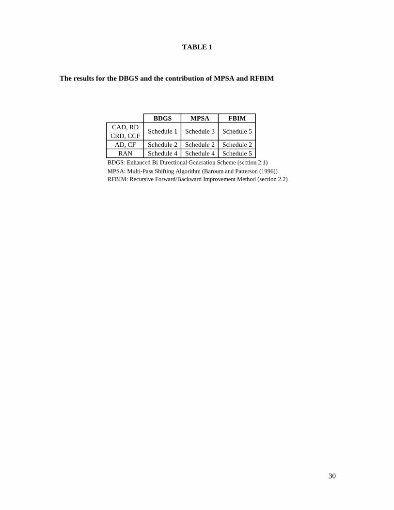
2.3 An illustrative example

In this section, we illustrate the different versions of the bi-directional generation

scheme on a project network example displayed in figure 1 with a pre-specified project

duration of δn = 29, an interest rate α = 0.01 and a fixed resource availability (a1, a2, a3, a4) =

(10, 10, 10, 10). We illustrate the various methods of section 2.1 in the generation scheme (the

enhanced bi-directional generation scheme BDGS) and the contribution of the multi-pass

forward/backward shifting algorithm (MPSA) of Baroum and Patterson (1996) and the

recursive forward/backward improvement method (FBIM) of section 2.2.

Insert Figure 1 About Here

Figure 2 displays five different schedules obtained by using the procedures mentioned

earlier. The schedules are the best schedules (with the highest net present value) obtained by

enumerating all possible random key vectors and transforming them to a schedule using the

bi-directional generation method under the different rules of section 2.1. Schedule 5 has the

highest net present value and is equal to the optimal schedule for the project network of figure

1.


Table 1 displays illustrative results. The BDGS column shows the results for the

enhanced bi-directional generation scheme of section 2.1 under the different rules. The table

shows that none of the rules is able to find the optimal solution, although the RAN approach

results in the best solution. The multi-pass shifting algorithm is able to improve schedule 1 by

shifting activity 4 with a positive cash flows towards the project start within its available

slack, resulting in schedule 3. The recursive forward/backward improvement method further

optimizes schedule 3 and schedule 4 to the optimal schedule 5. Note that the AD and CF

approaches are not able to find the optimal solution, since schedule 2 can never be improved

by shifting (sets of) activities.

13

Insert Table 1 About Here

Figure 3 illustrates the beneficial effect of the recursive forward/backward

improvement method on schedule 1 to obtain schedule 5. Figure 3 (a) shows the initial tree

taking both the precedence and resource relations of schedule 1 into account. A backward

recursion search detects a first set of activities {4} with a total positive net present value of

323*e-0.01*25. This set is shifted towards the project deadline within its available slack, tacking

both the precedence and resource relations into account, resulting in the modified tree of

figure 3 (b). A second backward run detects and shifts a second set {3, 4} with a total positive

net present value of -127*e-0.01*16 + 323*e-0.01*22 = 150.99, resulting in schedule 4 (figure

3(c)). A last backward search detects {5, 6, 7} to be shifted, resulting in the tree of figure 3

(d). The backward search is followed by a forward search. Since no sets of activities with a

negative net present value could be found, the recursive algorithm stops and returns schedule

5.


Note that the MPSA is only able to transform schedule 1 of figure 3(a) to schedule 3 of

figure 3(b) and then terminates. The extra arc between the dummy and activity and the

dummy start activity is necessary to connect two sub-trees in order to construct one tree. In

doing so, the recursive search can investigate all project activities during its search, both for

the forward step (starting from dummy start node 0) and the backward step (starting from

dummy end node 8).

14

3 SCATTER SEARCH PROCEDURE

Scatter search is an evolutionary method originally proposed by Glover (1998). The

basic as well as more advanced features of the scatter search meta-heuristic have been

presented in Glover and Laguna (2000) and Marti et al. (2006). The pseudo-code for any

general scatter search algorithm can be described as follows:

Algorithm Scatter Search Diversification Generation Method While Stop Criterion not met Improvement Method Reference Set Update Method Subset Generation Method Subset Combination Method End While

In the following sub-section, we describe our implementation of the scatter search

approach to solve the RCPSPDC taking the various principles of section 2 into account. In

section 3.2, we briefly discuss the dynamic update of three parameter values.

3.1 Our scatter search implementation

The Diversification Generation Method: In this initialization step, an initial pool of

solutions is generated by randomly generating random key (RK) vectors and constructing the

corresponding schedule using the bi-directional forward/backward generation scheme or the

well-known serial schedule generation scheme. If the former generation scheme fails in

constructing a schedule within the pre-defined deadline, the well-known serial generation

scheme is applied to generate a resource feasible schedule ignoring the pre-specified project

deadline. As a result, this obtained schedule might end before, on or behind the pre-specified

project deadline. After the schedule generation, information from the obtained schedule will

be used to transform the random key RK into a standardized random key (SRK). These

standardized random keys fulfil the topological order condition of Valls et al. (2003, 2004)

and follow the four guidelines of Debels and Vanhoucke (2006).

15

The Improvement Method: This local search step aims at improving all elements

from the pool of solutions, as follows:

• D-feasible solutions: these schedules are the subject to the recursive

forward/backward improvement method of section 2.2 in order to improve the

total net present value of the schedules.

• D-infeasible solutions: these schedules with a project duration larger than the

pre-defined project deadline are subject to the iterative forward/backward

scheduling technique of Li and Willis (1992). In doing so, the algorithm tries to

transform D-infeasible schedules into D-feasible schedules. If the resulting

project duration is smaller than or equal to the pre-specified project duration, the

obtained schedules are treated as D-feasible schedules, and hence, are the subject

to the recursive forward/backward improvement procedure as mentioned above.

The Reference Update Method: A reference set is created containing high-quality

and diverse solutions, with B1 ∩ B2 = ∅, as follows:

• The quality subset B1: contains the best solutions found since the start of the

procedure. This set only contains D-feasible schedules and has maximum b1

solution elements. In order to guarantee that the best known solutions are

diverse, a new schedule only enters the subset B1 if the minimal distance to any

existing element in the subset exceeds the threshold t1 or when the new candidate

solution is better than any generated solution so far.

• The diversity subset B2: contains D-feasible solutions that are sufficiently

different from the D-feasible solutions in subset B1 and/or D-infeasible schedules

with a project makespan larger than its pre-defined deadline. This set contains

exactly b2 solution elements (since the B2 set also allows D-infeasible solutions,

the number of elements is always equal to its maximal value). The divergence

between D-feasible elements in B1 and B2 is guaranteed by a threshold value t2

which is the minimal required distance between the candidate solution and any

element of B1.

The parameter values t1 and t2 are dynamically updated throughout the search process,

as explained in section 3.2. This two-tier design is maintained throughout the whole search of

the procedure. While the B1 subset contains the best known solutions so far, the B2 subset is

re-constructed from scratch during each run. Hence, all original elements are removed before

the reference set update method begins.

16

The Subset Generation Method: The scatter search procedure operates on the

reference set by combining pairs of solutions in a controlled way. The algorithm creates new

solutions from all two-element subsets as follows:

• B1 × B1: evaluation of all pairs of elements from B1 containing at least one new

solution compared to the previous generation. This method stimulates

intensification since it selects two reference solutions from the same cluster.

• B1 × B2: evaluation of all pairs combining an element from B1 and an element

from B2. This method stimulates diversification since it selects two reference

solutions from a different cluster.

• B2 × B2: evaluation of all pairs of elements from B2. This generation method is

only executed when the number of solution elements in B1 is lower than a

threshold value t3 (with t3 ≤ b1), and is particularly useful for project instances

with a low deadline or tight resource constraints. In doing so, this method

stimulates the generation of D-feasible solutions and aims at the increase of the

number of solution elements in subset B1. Unlike the dynamic update of the

parameter values t1 and t2, t3 is fixed throughout the search process (see section

3.2).

The Subset Combination Method: In order to combine solution elements from the

different subsets, we have implemented two straightforward crossover operators, which are

both used depending on the origin of the sets in the subset generation method.

• Two reference solutions from the same cluster (B1 × B1 and B2 × B2): The two-

point crossover randomly selects two crossover points from the interval c1 ∈ [0,

n – cmin] and c2 ∈ [c1 + cmin, n] with cmin the minimal number of activities subject

to a change. Two child solutions are constructed by exchanging all SRK values

between c1 and c2 between the parents. Activities that are not subject to a change

are modified in order to preserve the relative ranking of these activities. More

precisely, they get an SRK value equal to its original SRK value plus (minus) a

large constant when its original value is higher (lower) than c2 (c1).

17

• Two reference solutions from a different cluster (B1 × B2): The cash flow

crossover combines information from both parents into a single child solution as

follows: the crossover operator scans all SRK values of the father and the mother

and copies the lowest (largest) SRK value in to the child solution when the cash

flow of the corresponding activity is positive (negative). This approach aims at

combining the best characteristics from two diverse solution elements, one from

B1 and another from the B2 cluster with a minimal diversity of t2.

3.2 Dynamic parameter settings

In section 3.1, we have defined three different threshold parameters with each a

different function. The t1 and t1 parameters represent minimal distance values between two

solutions while the t3 is a parameter to guide the subset generation method. The distance

between two solutions x and y represented by their corresponding vectors SRKx and SRKy is

measured as the sum of the absolute values of the component-wise difference between all

vector elements of SRKx and SRKy.

The threshold parameter t1 represents the minimal required distance between a

candidate solution for subset B1 and all existing solutions in B1. In the beginning of the search

process, the number of D-feasible elements in B1 is low (initially equal to zero), and hence,

the threshold needs to be set very low in order to allow the entrance of any D-feasible solution

that is (sometimes only slightly) different than the current existing solutions. However, when

the search process continues, the number of D-feasible elements in B1 will likely to increase

(up to its maximum of b1), and hence, the algorithm need to increase the threshold value t1 in

order to guarantee more diverse high-quality schedules. However, the rate in which the

number of solution elements in B1 increases depends on factors such as the project deadline

(finding D-feasible schedules within tight project deadlines is extremely complex) and the

resource constrainedness. Once the number of D-feasible elements in B1 is equal to its

maximum value b1, the threshold value t1 can be decreased again depending on the number of

new solution elements newb1 of B1 during the previous run of the reference update method. In

doing so, the algorithm continually increases or decreases its threshold value along its search.

The threshold value can be calculated as newttb

b

distdistt 1

1

minmax

1 *11−

= . The values for min1t

dist

( max1t

dist ) represent the minimal (maximal) threshold values between which t1 varies linearly

and have been set to 1 and 2 * n, respectively.

18

The threshold parameter t2 represents the minimal required distance between a

candidate solution of B2 and any element of B1. The dynamic calculation of the threshold

value t2 follows a similar reasoning as t1 and depends on the number of D-feasible new

solution elements newb2 in B2 during the previous run of the reference update method. The

threshold value can be calculated as newttb

b

distdistt 2

2

minmax

2 *22−

= . The values for min2t

dist

( max2t

dist ) represent the minimal (maximal) threshold values between which t2 varies linearly

and have been set to 1 and 10 * n, respectively.

The threshold parameter t3 represents the minimal number of solution elements in B1

necessary to finish the B2 × B2 search in the subset generation method. In our implementation,

we have set t3 to a fixed value equal to b1 / 3.

4 COMPUTATIONAL RESULTS

In this section, we test the performance of the different solution procedures on two

randomly generated test sets consisting of resource-constrained project instances generated by

RanGen (Demeulemeester et al. 2003). Each project instance has been extended by activity

cash flows and a project deadline.

4.1 Full enumeration

In this section, we compare the performance of the various generation schemes on the

first test set by enumerating all possible random keys that fulfil the topological order

condition. Due to the huge amount of different possible keys, this experiment is restricted to

project instances with 10 activities.

The test instances has been generated by RanGen (Demeulemeester et al., 2003) as

follows: each instance contains 10 non-dummy activities with each duration randomly

generated between 1 and 10. Each project instance has an order strength OS and a resource-

constrainedness RC fixed at 0.25, 0.50, or 0.75. All project instances have 4 different resource

types with availabilities of 10 units and have a resource use equal to two (each activity needs

exact two of the four resources). The project deadline has been set to the minimal resource-

constrained project deadline (obtained by the procedure of Demeulemeester and Herroelen

(1993)) or to this minimal deadline exceeded by 5 time units.

19

The cash flows have been generated between [-500, 500] such that the percentage of

negative cash flows varies between 0% and 100% in steps of 10%. Using 10 instances for

each problem setting, we obtain a problem set of 3 * 3 * 2 * 11 * 10 = 1920 network

instances.

In order to measure the quality of the generation scheme under study, we calculate the

average deviation between the resulting heuristic solutions npvheur and the optimal solution

npvopt obtained by the procedure of Vanhoucke et al. (2001), as opt

heuropt

npvnpv

npvnpv −=∆ . We

also display the percentage of feasible solutions found for each problem instance as the total

number of feasible solutions found divided by the total number of evaluated priority vectors.

Table 2 reports the results for the generation schemes (forward (FOR), backward

(BAC) or bi-directional (all remaining columns)) with (yes) or without (no) the recursive

improvement method of section 2.2. The bi-directional generation scheme has been

implemented using the different third option rules of section 2.1. The table reveals that the

simple forward and backward schedule generation scheme perform poor and generate

heuristic solutions that deviate from the optimal solution with approximately 5% (without the

recursive improvement method) and 3% (with the recursive improvement method). Moreover,

the results show that the use of the bi-directional scheme improves the results dramatically,

although some versions are still not able to generate the optimal solution under full

enumeration. The resource-based approach (RS and CRS) perform less good than the activity

duration based approach (AD and CAD) which is, on its turn, outperformed by the cash flow

based approach (CF and CCF). Note that we also have tested the discounted cash flow

approach of Selle and zimmermann (2003) (not shown in the table), which reveals similar

results than the CF approach of table 2. However, optimal solutions can only be generated by

the random approach (RAN) which shows the best results. Finally, the table clearly shows that

the use of the recursive improvement method leads to improved results for all approaches in

the table.


20

Table 3 displays the average percentage of D-feasible solutions found per problem

instance. Since we have found that the percentage negative cash flows has no significant

influence on the number of D-feasible solutions, it is not included in table 3.


First, the table clearly reveals that infeasibilities occur more often when the order

strength is low and the resource-constrainedness is high. Selle and Zimmermann (2003) have

shown that their bi-directional generation scheme is not always able to generate D-feasible

instances and the likelihood for infeasibilities increases with tight resource constraints. The

decreasing complexity for the order strength has been noted by various authors (see e.g.

Herroelen and De Reyck (1999) and Demeulemeester et al. (2003), amongst others). Second,

the table shows that a project scheduling problem with a strict deadline is more complex than

the same scheduling problem with a larger deadline. It is intuitively clear that a project

instance with a strict deadline leads to more D-infeasible schedules than a similar instance

with more scheduling freedom. Finally, we note that the results differ only slightly between

the different versions of all generation schemes. The minimal overall value is equal to

75.88% (the AD approach) while the maximal value equals 78.99% (the FOR approach). This

is, however, not shown in table 3.

4.2 Scatter search

In this section, we present detailed computational results to test the performance of the

scatter search algorithm and compare the obtained results with optimal or best known feasible

solutions. Moreover, we present a randomly generated dataset containing 17,280 RCPSPDC

instances that can be downloaded from our website for future research purposes.

The test instances has been generated by RanGen (Demeulemeester et al. 2003) under

the settings displayed in table 4. The project deadline has been set to the minimal resource-

constrained project deadline exceeded by a certain percentage of this project duration (see

table).

21

In order to find the minimal project deadline, we have used the branch-and-bound

procedure of Demeulemeester and Herroelen (1993) for the 25-activity instances and the

decomposition-based genetic algorithm of Debels and Vanhoucke (2006) for all other

instances truncated after 100,000 generated schedules. Hence, the minimal project deadlines

for the 50, 75 and 100-activity instances are not necessarily optimal. Using 10 instances for

each problem setting, we obtain a problem set of 4 * 3 * 3 * 2 * 4 * 6 * 10 = 17,280 problem

instances.


Table 5 displays the results for the 25-activity instances and compares the solutions

obtained by the branch-and-bound procedure of Vanhoucke et al. (2001) with the heuristic

solutions obtained by our scatter search procedures truncated after 5,000 generated schedules

and by a random multi-start heuristic. The branch-and-bound procedure has been truncated

after a pre-specified time limit of 100 seconds, which results in three classes of solutions:

optimal, feasible and infeasible solutions. The optimal solutions have been found within the

pre-specified time limit. The feasible solutions have been reported after truncation and cannot

be proven to be optimal. If after the time limit no feasible solution can be found, this solution

enters the class of infeasible solutions. The multi-start heuristic randomly generates 5,000

random key vectors that are transformed into a schedule by the bi-directional generation

scheme and improved by the recursive forward/backward improvement method. The heuristic

solutions obtained by the scatter search procedure and the multi-start heuristic are compared

with all solutions from these three classes. Furthermore, we report whether the heuristic

solution is worse (lower net present value, denoted by “–“), equal (“=”) or better (higher net

present value, or “+”) than the corresponding solution obtained by the BB procedure. The

different runs correspond with different versions of the scatter search procedure, as follows:

22

• Run 1: Scatter search with iterative forward/backward algorithm of Li and Willis

(1992)

• Run 2: Scatter search with iterative forward/backward algorithm of Li and Willis

(1992) followed by the recursive forward/backward improvement method of

section 2.2

• Run 3: Scatter search with the bi-directional generation scheme (with a random

choice for the third option)

• Run 4: Scatter search with the bi-directional generation scheme (random choice)

followed by the recursive forward/backward improvement method of section 2.2.


The table reveals the following encouraging results. First, the comparison between the

multi-start rows and the scatter search – run4 reveals that the scatter search procedure

outperforms the multi-start heuristic (both procedures work with the bi-directional generation

scheme (random choice) followed by the recursive forward/backward improvement method).

Second, the scatter search procedure never leads to infeasible solutions, and the beneficial

effect of the bi-directional generation scheme and the recursive improvement method is

highlighted by the increasing number of solutions that are equal (better) than the solutions

obtained by the truncated branch-and-bound procedure. While the run1 version still has

36.60% + 32.94% = 69.54% solutions that are worse that the B&B solutions, the run4 version

has decreased that number to 14.63%. 6.74% (12.52%) of the solutions are equal to (better

than) the truncated B&B solution for the run1 version, and this number increases to 36.55%

(37.62%) for the run4 version. Last, note that the results are obtained after an average CPU

time of 2.19 seconds, while the B&B solutions have an average run time of 65.21 seconds

(truncated after 100 seconds).

Table 6 displays the solutions found by our scatter search algorithm truncated after

1,000, 5,000 and 50,000 schedules and acts as best known heuristic solutions with can be used

to compare newly found solutions in the future. The solution quality has been displayed as the

average percentage deviation (%Dev) from the optimal net present value of the corresponding

project scheduling problem instance ignoring the resource constraints.

23

This so-called max-npv problem has been solved by the efficient recursive search

method described in Vanhoucke (2006). We advice future researchers to test their procedures

on the same benchmark set and to report their results in a similar way as in table 6. All

detailed results, executables, test instances and detailed information can be downloaded from

our website www.projectmanagement.ugent.be/npv.php.


Note that the b1 and b2 values depend on the stop criterion and have been set to 10

and 5 for 1,000 schedules, 25 and 10 for 5,000 schedules and 50 and 30 for 50,000 schedules.

Other parameters are stop criterion independent: the number of initial solution elements in the

diversification generation method is always equal 500 and the minimum number of activities

subject to a change in the subset combination method equals cmin = n / 5.

24

5 CONCLUSIONS

In this paper, we presented a scatter search algorithm to solve the resource-constrained

project scheduling problem with discounted cash flows. This meta-heuristic procedure makes

use of a bi-directional generation scheme and a recursive forward/backward improvement

method.

We have tested various variants of our algorithm on a self generated dataset containing

17,280 problem instances. We have illustrated the contribution of the bi-directional generation

scheme and the beneficial effect of the recursive forward/backward improvement method. In

order to facilitate comparison for future research developments, we have reported best known

solutions under three different stop criteria and created a website where all detailed

information can be downloaded.

Our future intentions are as follows: First, we want to develop more advanced meta-

heuristic search procedures to extend the basic problem type to, for example, multi-mode

scheduling problems, pre-emptive activity execution, variable cash flows and many more. We

believe that enhanced versions of the bi-directional generation scheme and the recursive

forward/backward improvement method can still be used for more advanced problem

formulations. Second, we want to test our procedure on real-life instances. As an example,

Vanhoucke and Demeulemeester (2003) have shown the beneficial effect of net present value

maximization on a real-life capacity expansion project at a Flemish company that purifies

water. Last, we want to compare the scatter search framework with the building blocks of

other meta-heuristics, such as genetic algorithms, particle swarm optimization, ant colony

optimization, etc… and compare their performance on our proposed dataset.

25

REFERENCES

Baroum, S.M. and Patterson, J.H., 1996, “The development of cash flow weight procedures

for maximizing the net present value of a project”, Journal of Operations Management, 14,

209-227.

Brucker, P., Drexl, A., Möhring, R., Neumann, K. and Pesch, E., 1999, “Resource-constrained

project scheduling: notation, classification, models and methods”, European Journal of

Operational Research, 112, 3-41.

Debels, D. and Vanhoucke, M., 2006, “A decomposition-based genetic algorithm for the

resource-constrained project scheduling problem”, to appear in Operations Research

Demeulemeester, E., Vanhoucke, M., and Herroelen, W., 2003, “A random network generator

for activity-on-the-node networks”, Journal of Scheduling, 6, 13-34.

De Reyck, B. and Herroelen, W., 1998, “Optimal procedure for the resource-constrained

project scheduling problem with discounted cash flows and generalized precedence relations”,

Computers and Operations Research, 25, 1-17.

Glover, F, 1998, “A Template for Scatter Search and Path Relinking”, Lecture Notes in

Computer Science, 1363, 13-54

Glover, F. and Laguna, M., 2000, “Fundamentals of Scatter Search and Path Relinking”,

Control and Cybernetics, 3, 653-684.

Herroelen, W. and De Reyck, B., 1999, “Phase transitions in project scheduling”, Journal of

the Operational Research Quarterly, 50, 148-156.

Herroelen, W., De Reyck, B. and Demeulemeester, E., 1998, “Resource-constrained project

scheduling: a survey of recent developments”, Computers and Operations Research, 25, 279-

302.

Icmeli, O., Erenguc, S.S. and Zappe, C.J., 1993, “Project scheduling problems: a survey”,

International Journal of Operations and Productions Management, 13, 80-91.

26

Kolisch, R. and Hartmann, S., 2005, “Experimental investigation of Heuristics for resource-

constrained project scheduling: an update”, European Journal of Operational Research, to

appear.

Kolisch, R. and Padman, R., 2001, “An integrated survey of deterministic project scheduling”,

Omega, 49, 249-272.

Marti, R., Laguna, M. and Glover, F., 2006, “Principles of scatter search”, European Journal

of Operational Research, 169, 359-372.

Özdamar, L. and Ulusoy, G., 1995, “A survey on the resource-constrained project scheduling

problem”, IIE Transactions, 27, 574-586.

Özdamar, L., Ulusoy, G. and Bayyigit, M., 1998, “A heuristic treatment of tardiness and net

present value criteria in resource-constrained project scheduling”, International Journal of

Physical Distribution and Logistics, 28, 805-824.

Padman, R. and Smith-Daniels, D.E., 1993, “Early-tardy cost trade-offs in resource

constrained projects with cash flows: An optimization-guided heuristic approach”, European

Journal of Operational Research, 64, 295-311.

Padman, R., Smith-Daniels, D.E. and Smith-Daniels, V.L., 1997, “Heuristic scheduling of

resource-constrained projects with cash flows”, Naval Research Logistics, 44, 365-381.

Pinder, J.P. and Marucheck, A.S., 1996, “Using discounted cash flow heuristics to improve

project net present value”, Journal of Operations Management, 14, 229-240.

Russell, R.A., 1986, “A comparison of heuristics for scheduling projects with cash flows and

resource restrictions”, Management Science, 32, 1291-1300.

Schwindt, C. and Zimmermann, J., 2001, “A steepest ascent approach to maximizing the net

present value of projects”, Mathematical Methods of Operations Research, 53, 435-450.

Selle, T. and Zimmermann, J., 2003, “A bidirectional heuristic for maximizing the net present

value of large-scale projects subject to limited resources”, Naval Research Logistics, 50, 130-

148.

27

Ulusoy, G. and Özdamar, L., 1995, “A heuristic scheduling algorithm for improving the

duration and net present value of a project”, International Journal of Operations and

Production Management, 15, 89-98.

Vanhoucke, M., 2006, “An efficient hybrid search procedure for various optimization

problems”, Lecture Notes on Computer Science, 3906, 272-283

Vanhoucke, M. and Demeulemeester, E., 2003, “The Application of Project Scheduling

Techniques in a Real-Life Environment”, Project Management Journal, 34, 30-42.

Vanhoucke, M., Demeulemeester, E. and Herroelen, W., 2001, “On maximizing the net

present value of a project under renewable resource constraints”, Management Science, 47,

1113-1121.

Yang, K.K., Tay, L.C. and Sum, C.C., 1995, “A comparison of stochastic scheduling rules for

maximizing project net present value”, European Journal of Operational Research, 85, 327-

339.

Zhu, D. and Padman, R. A cooperative multi-agent approach to constrained project

scheduling. Interfaces in Computer Science and Operations Research: Advances in

Metaheuristics, Optimization, and Stochastic Modeling Technologies eds. R.S. Barr, R.V.

Helgason, and J.L. Kennington, Kluwer Academic Publishers, Norwell, MA, 367-381, 1997.

Zhu, D. and Padman, R., 1999, “A metaheuristic scheduling procedure for resource-

constrained projects with cash flows”, Naval Research Logistics, 46, 912-927.

28

FIGURE 1

An example project network

0,0,0,0

00

11

22

55

33

66

77

44 88

0,0 0,0,1,1

2,227

1,0,10,0

9,426

0,5,3,0

1,-263

5,1,0,0

1,-127 8,0,6,0

6,323

0,9,0,7

8,250

6,0,0,7

4,344

0,0,0,0

0,0

ii

ri1,ri2,ri3,ri4

di, cfi

29

FIGURE 2

Five different schedules obtained by different procedures

1234567

1234567

1234567

1234567

1234567

1 2 3 4 5 6 7 8 9 10 11 12 13 14 15 16 17 18 19 20 21 22 23 24 25 26 27 28 29

Schedule 5: DC = 1020.69





30

TABLE 1

The results for the DBGS and the contribution of MPSA and RFBIM

BDGS: Enhanced Bi-Directional Generation Scheme (section 2.1)

MPSA: Multi-Pass Shifting Algorithm (Baroum and Patterson (1996))RFBIM: Recursive Forward/Backward Improvement Method (section 2.2)

CAD, RDCRD, CCF

AD, CFRAN

Schedule 1 Schedule 3 Schedule 5

Schedule 2Schedule 4



BDGS MPSA FBIM

31

FIGURE 3

The recursive forward/backward (backward part) search on schedule 1

(straight lines represent precedence relations and dotted lines represent resource relations)

0

1

2

5

3

6

7

4 8

f3 = 16f2 = 11

f1 = 2

f0 = 0

f5 = 25

f4 = 25

f7 = 24

f8 = 29

f6 = 29

00

11

22

55

33

66

77

44 88

f3 = 16f2 = 11

f1 = 2

f0 = 0

f5 = 25

f4 = 25

f7 = 24

f8 = 29

f6 = 29

0

1

2

5

3

6

7

4 8

f3 = 16f2 = 11

f1 = 2

f0 = 0

f5 = 25

f4 = 22

f7 = 24

f8 = 29

f6 = 29

00

11

22

55

33

66

77

44 88

f3 = 16f2 = 11

f1 = 2

f0 = 0

f5 = 25

f4 = 22

f7 = 24

f8 = 29

f6 = 29

0

1

2

5

3

6

7

4 8

f3 = 12f2 = 11

f1 = 2

f0 = 0

f5 = 25

f4 = 18

f7 = 24

f8 = 29

f6 = 29

00

11

22

55

33

66

77

44 88

f3 = 12f2 = 11

f1 = 2

f0 = 0

f5 = 25

f4 = 18

f7 = 24

f8 = 29

f6 = 29

0

1

2

5

3

6

7

4 8

f3 = 12f2 = 11

f1 = 2

f0 = 0

f5 = 21

f4 = 18

f7 = 20

f8 = 29

f6 = 25

00

11

22

55

33

66

77

44 88

f3 = 12f2 = 11

f1 = 2

f0 = 0

f5 = 21

f4 = 18

f7 = 20

f8 = 29

f6 = 25

(a) Schedule 1 (b) Schedule 3

(c) Schedule 4 (d) Schedule 5

32

TABLE 2

Average deviation npv∆ from the optimal solution (in %)

no yes no yes no yes no yes no yes no yes no yes no yes no yesOverall 0.133 0.005 0.310 0.036 0.766 0.065 0.321 0.020 0.036 0.020 0.123 0.023 0.005 0.000 4.668 2.247 5.763 3.159

0.25 0.108 0.008 0.251 0.061 0.709 0.105 0.369 0.020 0.013 0.000 0.118 0.046 0.000 0.000 5.359 2.361 6.826 3.552

0.50 0.081 0.005 0.345 0.029 0.695 0.074 0.289 0.010 0.062 0.037 0.128 0.018 0.013 0.000 4.920 1.936 5.243 2.941

0.75 0.209 0.003 0.334 0.019 0.895 0.015 0.303 0.028 0.034 0.024 0.123 0.006 0.002 0.000 3.725 2.445 5.221 2.985

0.25 0.194 0.000 0.382 0.001 1.035 0.004 0.551 0.001 0.017 0.000 0.149 0.000 0.004 0.000 6.975 1.954 8.754 3.219

RC 0.50 0.124 0.011 0.324 0.085 0.734 0.155 0.246 0.045 0.015 0.001 0.130 0.052 0.000 0.000 4.390 2.863 5.666 3.748

0.75 0.080 0.004 0.224 0.023 0.530 0.034 0.166 0.013 0.078 0.061 0.090 0.018 0.010 0.000 2.639 1.926 2.870 2.511

0 0.010 0.003 0.039 0.014 0.153 0.037 0.083 0.001 0.029 0.025 0.033 0.022 0.001 0.000 2.988 0.566 3.320 0.922

5 0.256 0.008 0.581 0.058 1.379 0.093 0.559 0.039 0.044 0.016 0.213 0.024 0.009 0.000 6.348 3.929 8.207 5.396

0 0.000 0.000 0.000 0.000 0.000 0.000 0.000 0.000 0.000 0.000 0.000 0.000 0.000 0.000 0.000 0.000 3.957 1.956

10 0.000 0.000 0.000 0.000 0.000 0.000 0.000 0.000 0.000 0.000 0.000 0.000 0.000 0.000 1.592 0.847 4.554 2.591

20 0.000 0.000 0.000 0.000 0.000 0.000 0.000 0.000 0.000 0.000 0.000 0.000 0.000 0.000 1.592 0.847 4.554 2.591

30 0.000 0.000 0.000 0.000 0.000 0.000 0.000 0.000 0.000 0.000 0.000 0.000 0.000 0.000 1.592 0.847 4.554 2.591

40 0.125 0.004 0.171 0.011 0.658 0.048 0.293 0.021 0.035 0.026 0.091 0.018 0.004 0.000 4.075 1.962 6.214 3.554

50 0.125 0.004 0.171 0.011 0.658 0.048 0.293 0.021 0.035 0.026 0.091 0.018 0.004 0.000 4.075 1.962 6.214 3.554

60 0.125 0.004 0.171 0.011 0.658 0.048 0.293 0.021 0.035 0.026 0.091 0.018 0.004 0.000 4.075 1.962 6.214 3.554

70 0.446 0.018 1.244 0.166 2.945 0.262 1.158 0.055 0.128 0.070 0.449 0.090 0.020 0.000 10.705 4.900 11.943 6.221

80 0.446 0.018 1.244 0.166 2.945 0.262 1.158 0.055 0.128 0.070 0.449 0.090 0.020 0.000 10.705 4.900 11.943 6.221

90 0.193 0.007 0.407 0.032 0.565 0.044 0.333 0.042 0.038 0.007 0.183 0.022 0.004 0.000 8.432 4.262 3.248 1.920

100 0.000 0.000 0.000 0.000 0.000 0.000 0.000 0.000 0.000 0.000 0.000 0.000 0.000 0.000 4.503 2.232 0.000 0.000

OS

Deadline

%Neg

AD CAD RD CRD BACCF CCF RAN FOR

33

TABLE 3

Average percentage of D-feasible solutions per problem instance

0.25 0.50 0.75 0.25 0.50 0.75Deadline

0.25 85.26 38.12 22.71 99.78 82.77 70.980.50 95.38 49.37 37.12 100.00 90.45 73.440.75 100.00 66.98 72.85 100.00 93.46 94.19

RC

OS

0 5

34

TABLE 4

Parameter settings used to generate the test instances for the RCPSPDC

Numer of activities 25, 50, 75 or 100

Activity durations Randomly selected from the interval [1, 10]

Order strength OS 0.25, 0.50 or 0.75

Number of resource types 4

Resource constrainedness RC 0.25, 0.50 or 0.75

Resource use RU 2 or 4

Project deadline 5, 10, 15 or 20

Discount rate α 0.01

Percentage negative cash flows 0, 20, 40, 60, 80 or 100

35

TABLE 5

Computational results for the 25 activity networks

infeasible feasible optimal11.20% 49.86% 38.94%

– 60.30% × 36.97% 23.33%= 15.95% 0.23% 0.12% 15.60%+ 23.75% 10.97% 12.78% ×– 69.51% × 36.57% 32.94%= 6.74% 0.00% 0.74% 6.00%+ 23.75% 11.20% 12.55% ×– 67.36% × 35.21% 32.15%= 7.52% 0.00% 0.74% 6.78%+ 25.12% 11.20% 13.91% ×– 21.23% × 7.66% 13.56%= 30.23% 0.00% 4.86% 25.37%+ 48.54% 11.20% 37.34% ×– 13.89% × 5.95% 7.94%= 37.08% 0.00% 6.09% 31.00%+ 49.03% 11.20% 37.82% ×

B&B

Run

1R

un 2

Run

3R

un 4

Mul

ti

Sta

rtS

catte

r S

earc

h

36

TABLE 6

Computational experience for 1,000, 5,000 and 50,000 schedules

%Dev CPU %Dev CPU %Dev CPUOverall 234.57 1.28 224.94 2.19 215.86 13.08

25 193.93 0.36 191.69 0.55 190.49 2.5850 305.93 0.84 295.14 1.42 286.26 8.1475 185.91 1.50 173.38 2.57 162.27 15.38100 252.50 2.42 239.56 4.24 224.42 26.210.25 208.12 1.40 193.05 2.31 179.51 12.960.50 228.46 1.21 222.17 2.08 213.69 12.660.75 267.13 1.23 259.60 2.19 254.38 13.610.25 100.27 1.58 92.93 2.71 84.90 16.34

RC 0.50 368.58 1.11 353.94 1.91 342.64 11.500.75 234.85 1.15 227.96 1.96 220.05 11.39

2 273.78 1.32 262.48 2.34 252.64 14.564 195.35 1.24 187.40 2.05 179.09 11.605 272.15 0.85 265.37 1.55 257.34 9.9710 160.74 1.10 152.35 1.94 143.72 11.9515 344.38 1.47 332.34 2.47 321.41 14.3220 160.996 1.697 149.713 2.815 140.975 16.070 31.78 0.86 31.42 1.40 30.93 7.6820 30.08 0.94 29.56 1.50 28.78 8.0040 72.69 1.14 70.35 1.85 67.59 10.0060 494.29 1.35 478.38 2.32 463.79 13.7780 483.82 1.56 454.59 2.77 429.57 17.20100 294.74 1.83 285.35 3.34 274.50 21.81

Deadline

%Neg

SS (50,000)

RU

OS

Act

SS (1,000) SS (5,000)

A SCATTER SEARCH PROCEDURE FOR MAXIMIZING THE NET PRESENT ...

Documents

Transcript of A SCATTER SEARCH PROCEDURE FOR MAXIMIZING THE NET PRESENT ...