ATTENUATION, SCATTER, AND SPATIAL RESOLUTION COMPENSATION ... Scatter, and... · King, et al,...
56
King, et al, Attenuation, Scatter, and Resolution Compensation in SPECT 1 ATTENUATION, SCATTER, AND SPATIAL RESOLUTION COMPENSATION IN SPECT By Michael A. King, Stephen J. Glick, P. Hendrik Pretorius, R. Glenn Wells, Howard C. Gifford, Manoj V. Narayanan, and Troy Farncombe Division of Nuclear Medicine Department of Radiology The University of Massachusetts Medical School 55 Lake Ave North Worcester, MA 01655 I. Review of the Sources of Degradation and Their Impact in SPECT Reconstruction A. Ideal imaging B. Sources of image degradation C. Impact of degradations II. Non-uniform Attenuation Compensation A. Estimation of patient-specific attenuation maps B. Compensation methods for correction of non-uniform attenuation C. Impact of non-uniform attenuation compensation on image quality III. Scatter Compensation A. Scatter estimation methods B. Reconstruction-based scatter compensation (RBSC) methods C. Impact of scatter compensation on image quality IV. Spatial Resolution Compensation A. Restoration filtering B. Modeling spatial resolution in iterative reconstruction C. Impact of resolution compensation on image quality V. Conclusions VI. Acknowledgments VII. References I. Review of the Sources of Degradation and Their Impact in SPECT Reconstruction A. Ideal imaging Data acquisition for the case of ideal SPECT imaging is illustrated in Figure 1, which portrays a single-headed gamma camera imaging a source distribution f(x,y) at a rotation angle θ with respect to the x-axis. The camera is equipped with a parallel-hole absorptive collimator, which for this ideal case only allows photons emitted from f(x,y) in a direction parallel to the collimator septa to pass through to the NaI(Tl) crystal, and be detected. The source distribution in Figure 1 is a cartoon drawing of a slice through the three-dimensional (3D) mathematical cardiac-torso (MCAT) phantom [1] with a Tc-99m sestamibi distribution. Let (t, s) be a coordinate system rotated by the angle θ counter-clockwise with
Transcript of ATTENUATION, SCATTER, AND SPATIAL RESOLUTION COMPENSATION ... Scatter, and... · King, et al,...
King, et al, Attenuation, Scatter, and Resolution Compensation in SPECT 1
ATTENUATION, SCATTER, AND SPATIAL RESOLUTION COMPENSATION IN SPECT
By
Michael A. King, Stephen J. Glick, P. Hendrik Pretorius, R. Glenn Wells, Howard C. Gifford, Manoj V.Narayanan, and Troy Farncombe
Division of Nuclear MedicineDepartment of Radiology
The University of Massachusetts Medical School55 Lake Ave North
Worcester, MA 01655
I. Review of the Sources of Degradation and Their Impact in SPECT ReconstructionA. Ideal imagingB. Sources of image degradationC. Impact of degradations
II. Non-uniform Attenuation CompensationA. Estimation of patient-specific attenuation mapsB. Compensation methods for correction of non-uniform attenuationC. Impact of non-uniform attenuation compensation on image quality
III. Scatter CompensationA. Scatter estimation methodsB. Reconstruction-based scatter compensation (RBSC) methodsC. Impact of scatter compensation on image quality
IV. Spatial Resolution CompensationA. Restoration filteringB. Modeling spatial resolution in iterative reconstructionC. Impact of resolution compensation on image quality
V. ConclusionsVI. AcknowledgmentsVII. References
I. Review of the Sources of Degradation and Their Impact in SPECT Reconstruction
A. Ideal imaging
Data acquisition for the case of ideal SPECT imaging is illustrated in Figure 1, which portrays asingle-headed gamma camera imaging a source distribution f(x,y) at a rotation angle θ with respect to thex-axis. The camera is equipped with a parallel-hole absorptive collimator, which for this ideal case onlyallows photons emitted from f(x,y) in a direction parallel to the collimator septa to pass through to theNaI(Tl) crystal, and be detected. The source distribution in Figure 1 is a cartoon drawing of a slicethrough the three-dimensional (3D) mathematical cardiac-torso (MCAT) phantom [1] with a Tc-99msestamibi distribution. Let (t, s) be a coordinate system rotated by the angle θ counter-clockwise with
King, et al, Attenuation, Scatter, and Resolution Compensation in SPECT 2
respect to the (x, y) coordinate system. Then t and s can be written in terms of x and y, and the rotationangle θ as [2]:
t = x cos θ + y sin θ (1)s = -x sin θ + y cos θ .
The ray sum ( p(θ,t')) is the line integral over f(t,s) with respect to s for t = t', or
dydx)t-sinycos(xy)f(x,dsdt)t-(ts)(t,fdss),t(f)t,p( ′+=′=′=′ ∫ ∫∫ ∫∫∞
∞−
∞
∞−
∞
∞−
∞
∞−
∞
∞−
θθδδθ θθ , (2)
where δ is the delta function, and Equation 1 was used to express t in terms of x, y, and θ. The functionp(θ,t) for the case of ideal imaging is the Radon transform of f(x,y), and is the parallel projection of f(x,y)for a constant value of θ [3]. By rotating the camera head about the patient a set of projections is acquiredfor different projection angles. This set of projections constitutes the data that will be used to estimate thesource distribution from which they originated. Figure 2 shows the overlaid ideal projections of a pointsource in the liver of the MCAT phantom at projection angles of 00 (left lateral), 450 (left-anterioroblique), 900 (anterior), and 1350 (right-anterior oblique) relative to the x-axis in Figure 1. The location ofthe point source is indicated as the black circular point within the liver and on the x-axis in Figure 1.Notice in the ideal case, the projections are all of the same size and shape, and vary with projection anglejust in their positioning along the t-axis. When the projections are stacked one on top of the other forviewing, they form a matrix called the sinogram. The matrix is so named because with 360 degreeacquisitions each location traces out a sine function whose amplitude depends on the distance from thecenter-of-rotation (COR) and phase depends on its angular location.
B. Sources of image degradation
SPECT imaging is not ideal, however. Inherent in SPECT imaging are degradations, which distortthe projection data. This chapter will focus on three such degradations, and the compensation for them.The first is attenuation. In order for a photon to become part of a projection, it must escape the body. Asillustrated in Figure 3, photons emitted such that they would otherwise be detected may be eitherphotoelectrically absorbed (photon A) or scattered (photon B) such that they will be lost from inclusion inthe projections. Thus the attenuated projections (pA(θ,t)) will contain fewer events than the idealprojections. This is illustrated in Figure 4, which shows the attenuated projections of the point source ofFigure 2. Note how the reduction in the number of detected events varies with the thickness and nature ofmaterial through which the photons must travel to be imaged. The extent of attenuation can be quantifiedmathematically by the transmitted fraction (TF(t', s', θ)), which is the fraction of the photons fromlocation (t', s') that will be transmitted through a potentially non-uniform attenuator at angle θ. Thetransmitted fraction is given by:
)ds s),t((- exp ) ,s ,tTF(s∫∞
′
′=′′ µθ , (3)
King, et al, Attenuation, Scatter, and Resolution Compensation in SPECT 3
where µ(t,s) is the distribution of linear attenuation coefficients as a function of location. Equation 3 isaccurate only for a mono-energetic photon beam, and under the assumption that as soon as a photonundergoes any interaction, it is no longer counted as a member of the beam. The latter is the "goodgeometry" condition [4,5]. The attenuated projections are obtained from the ideal projections by includingTF within the integrals of Equation 2. As a result of the differences in attenuation coefficient with type oftissue, the TF will vary with the materials traversed even if the total patient thickness between the site ofemission and the camera is the same. That is, it makes a difference if the photons are passing throughmuscle, lung, or bone. Similarly, a change in TF will occur if the amount of tissue that has to be traversedis altered. Thus, one needs to have patient-specific information on the spatial distribution of attenuationcoefficients (an attenuation map or estimate of µ(t,s)) in order to calculate the attenuation that occurswhen photons are emitted from a given location in the patient and detected at a given angle.
The second source of degradation, which will be considered in this chapter, is the inclusion ofscatter in the projections. This, as is illustrated in Figure 5, leads to the inclusion of photons in theprojections that normally would not have been detected. Note that in Figure 6 a logarithmic scaling is usedfor the number of counts detected to better illustrate the contribution of scatter. To account for thepresence of scatter, Equation 3 can be modified by multiplying the exponential term by a buildup factor(B) [4]. The buildup factor is the ratio of the total number of counts detected within the energy window(primary plus scatter) to the number of primary counts detected within the window. In the “goodgeometry” case there is no scatter detected, so the buildup factor is 1.0. For the four point-sourceprojections in Figure 6 the buildup factors were 1.40 for the RAO view, 1.52 for the anterior view, 1.84for the left-anterior oblique view, and 2.21 for the left lateral view. Photons undergoing classicalscattering do not change energy during the interaction; thus they can not be separated from transmittedphotons on the basis of their energy. At the photon energies of interest in SPECT imaging, classicalscattering only makes up a small percentage of the interactions in the human body. Compton scattering isthe dominant mode of interaction under these conditions, and during Compton scattering the photon isreduced in energy as well as deflected from its original path. Thus one can use energy windowing toreduce the amount of scattered photons imaged, but not eliminate scatter, due to the presence of classicallyscattered photons and the finite energy resolution of current imaging systems. In fact, the ratio of scatteredto primary photons in the photopeak energy window (scatter fraction) is typically 0.34 for Tc-99m [6] and0.95 for Tl-201 [7]. When scatter is neither removed from the emission profiles prior to reconstruction norincorporated into the reconstruction process, it can lead to over-correction for attenuation because thedetected scattered photons violate the “good geometry” assumption of Equation 3.
The third source of degradation is the finite, distance-dependent spatial resolution of the imagingsystem. When imaging in air, the system spatial resolution consists of two independent sources of blurring[5]. The first is the intrinsic resolution of the detector and electronics, which is well modeled as aGaussian function. The second is the spatially varying geometrical acceptance of the photons through theholes of the collimator. This response is illustrated in Figure 7. Note in this figure that both photon A,which is emitted parallel to the s-axis, and photon B, which is angled relative to the s-axis, now make itthrough the collimator and are detected. Detailed theoretical analyses of the geometrical point-spread andtransfer functions for multihole collimators have been published [8-11]. In the absence of septalpenetration and scatter, the point-spread function (PSF) for parallel-hole collimators is typicallyapproximated as a Gaussian function [12-13] whose standard deviation (σC) is a linear function ofdistance given as:
σC (d) = σ0 + σd • d , (4)
King, et al, Attenuation, Scatter, and Resolution Compensation in SPECT 4
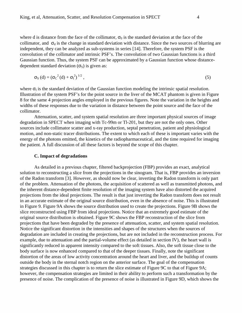
where d is distance from the face of the collimator, σ0 is the standard deviation at the face of thecollimator, and σd is the change in standard deviation with distance. Since the two sources of blurring areindependent, they can be analyzed as sub-systems in series [14]. Therefore, the system PSF is theconvolution of the collimator and intrinsic PSF’s. The convolution of two Gaussian functions is a thirdGaussian function. Thus, the system PSF can be approximated by a Gaussian function whose distance-dependent standard deviation (σS) is given as:
σS (d) = (σC2 (d) + σI
2) 1/2 , (5)
where σI is the standard deviation of the Gaussian function modeling the intrinsic spatial resolution.Illustration of the system PSF’s for the point source in the liver of the MCAT phantom is given in Figure8 for the same 4 projection angles employed in the previous figures. Note the variation in the heights andwidths of these responses due to the variation in distance between the point source and the face of thecollimator.
Attenuation, scatter, and system spatial resolution are three important physical sources of imagedegradation in SPECT when imaging with Tc-99m or Tl-201, but they are not the only ones. Othersources include collimator scatter and x-ray production, septal penetration, patient and physiologicalmotion, and non-static tracer distributions. The extent to which each of these is important varies with theenergy of the photons emitted, the kinetics of the radiopharmaceutical, and the time required for imagingthe patient. A full discussion of all these factors is beyond the scope of this chapter.
C. Impact of degradations
As detailed in a previous chapter, filtered backprojection (FBP) provides an exact, analyticalsolution to reconstructing a slice from the projections in the sinogram. That is, FBP provides an inversionof the Radon transform [3]. However, as should now be clear, inverting the Radon transform is only partof the problem. Attenuation of the photons, the acquisition of scattered as well as transmitted photons, andthe inherent distance-dependent finite resolution of the imaging system have also distorted the acquiredprojections from the ideal projections. The result is that just inverting the Radon transform does not resultin an accurate estimate of the original source distribution, even in the absence of noise. This is illustratedin Figure 9. Figure 9A shows the source distribution used to create the projections. Figure 9B shows theslice reconstructed using FBP from ideal projections. Notice that an extremely good estimate of theoriginal source distribution is obtained. Figure 9C shows the FBP reconstruction of the slice fromprojections that have been degraded by the presence of attenuation, scatter, and system spatial resolution.Notice the significant distortion in the intensities and shapes of the structures when the sources ofdegradation are included in creating the projections, but are not included in the reconstruction process. Forexample, due to attenuation and the partial-volume effect (as detailed in section IV), the heart wall issignificantly reduced in apparent intensity compared to the soft tissues. Also, the soft tissue close to thebody surface is now enhanced compared to that of the deeper tissues. Finally, note the significantdistortion of the areas of low activity concentration around the heart and liver, and the buildup of countsoutside the body in the sternal notch region on the anterior surface. The goal of the compensationstrategies discussed in this chapter is to return the slice estimate of Figure 9C to that of Figure 9A;however, the compensation strategies are limited in their ability to perform such a transformation by thepresence of noise. The complication of the presence of noise is illustrated in Figure 9D, which shows the
King, et al, Attenuation, Scatter, and Resolution Compensation in SPECT 5
FBP reconstruction of the degraded projections to which has been added Poisson noise typical of that inperfusion imaging.
The cause of the distortions in Figure 9C is the inconsistency of the projection data with the modelof imaging used in reconstruction. The model of the imaging system used with FBP reconstruction wasthat of an ideal imaging system (i.e., one with a PSF equal to a δ-function whose integral is a constantindependent of projection angle, as illustrated in Figure 2). The actual PSF’s for SPECT imaging vary inshape and magnitude with location in the slice and projection angle, as illustrated in Figure 8. Withoutcompensation for such variation prior to reconstruction, or accounting for the variation as part of thereconstruction algorithm, the reconstructed PSF is anisotropic with long positive and negative tails [15].The reason for this is as follows. Use of the “ramp” filter in FBP to compensate for the blurring ofbackprojection results in negative values in the projections. These negative values cancel out the wrongguesses as to where the counts are located when backprojected. If the acquired PSF’s are of different sizeand shape, then the cancellation is not exact, and a distorted reconstructed PSF results [16]. The low-magnitude tails of the reconstructed PSF’s from hot structures in images can add up, causing changes inthe apparent count level of nearby structures. Clinically, this can result in decreased apparent localizationin the inferior wall of the heart in perfusion images with significant hepatic activity [17], the loss of theability to visualize bone structures in bone scans at the level of significant bladder activity [18, 19], andother artifacts. The distortion is not limited to FBP, but occurs with iterative reconstruction if the imagingmodel is inconsistent with the actual data collection [16, 20].
II. Non-uniform Attenuation Compensation
A. Estimation of patient-specific attenuation maps
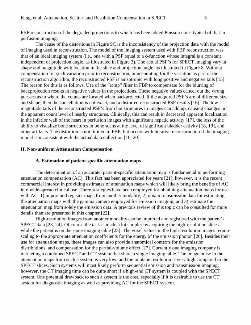
The determination of an accurate, patient-specific attenuation map is fundamental to performingattenuation compensation (AC). This fact has been appreciated for years [21]; however, it is the recentcommercial interest in providing estimates of attenuation maps which will likely bring the benefits of ACinto wide-spread clinical use. Three strategies have been employed for obtaining attenuation maps for usewith AC: 1) import and register maps from another modality; 2) obtain transmission data for estimatingthe attenuation maps with the gamma camera employed for emission imaging; and 3) estimate theattenuation map from solely the emission data. A previous review of this topic can be consulted for moredetails than are presented in this chapter [22].
High-resolution images from another modality can be imported and registered with the patient’sSPECT data [23, 24]. Of course the task is made a lot simpler by acquiring the high-resolution sliceswhile the patient is on the same imaging table [25]. The voxel values in the high-resolution images requirescaling to the appropriate attenuation coefficients for the energy of the emission photon [26]. Besides theiruse for attenuation maps, these images can also provide anatomical contexts for the emissiondistributions, and compensation for the partial-volume effect [27]. Currently one imaging company ismarketing a combined SPECT and CT system that share a single imaging table. The image noise in theattenuation maps from such a system is very low, and the in plane resolution is very high compared to theSPECT slices. Such systems will most likely perform sequential emission and transmission imaging;however, the CT imaging time can be quite short if a high-end CT system is coupled with the SPECTsystem. One potential drawback to such a system is the cost, especially if it is desirable to use the CTsystem for diagnostic imaging as well as providing AC for the SPECT system.
King, et al, Attenuation, Scatter, and Resolution Compensation in SPECT 6
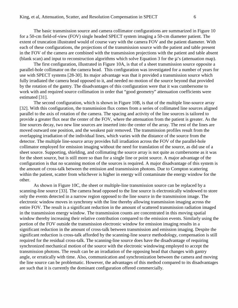
The basic transmission source and camera collimator configurations are summarized in Figure 10for a 50-cm field-of-view (FOV) single headed SPECT system imaging a 50-cm diameter patient. Theextent of truncation illustrated would of course vary with the camera FOV and the patient diameter. Witheach of these configurations, the projections of the transmission source with the patient and table presentin the FOV of the camera are combined with the transmission projections with the patient and table absent(blank scan) and input to reconstruction algorithms which solve Equation 3 for the µ’s (attenuation map).
The first configuration, illustrated in Figure 10A, is that of a sheet transmission source opposite aparallel-hole collimator on the camera head. This configuration was investigated for a number of years foruse with SPECT systems [28-30]. Its major advantage was that it provided a transmission source whichfully irradiated the camera head opposed to it, and needed no motion of the source beyond that providedby the rotation of the gantry. The disadvantages of this configuration were that it was cumbersome towork with and required source collimation in order that “good geometry” attenuation coefficients wereestimated [31].
The second configuration, which is shown in Figure 10B, is that of the multiple line-source array[32]. With this configuration, the transmission flux comes from a series of collimated line sources alignedparallel to the axis of rotation of the camera. The spacing and activity of the line sources is tailored toprovide a greater flux near the center of the FOV, where the attenuation from the patient is greater. As theline sources decay, two new line sources are inserted into the center of the array. The rest of the lines aremoved outward one position, and the weakest pair removed. The transmission profiles result from theoverlapping irradiation of the individual lines, which varies with the distance of the source from thedetector. The multiple line-source array provides full irradiation across the FOV of the parallel-holecollimator employed for emission imaging without the need for translation of the source, as did use of asheet source. Supporting, shielding, and collimating the source array is not quite as cumbersome as it wasfor the sheet source, but is still more so than for a single line or point source. A major advantage of theconfiguration is that no scanning motion of the sources is required. A major disadvantage of this system isthe amount of cross-talk between the emission and transmission photons. Due to Compton scatteringwithin the patient, scatter from whichever is higher in energy will contaminate the energy window for theother.
As shown in Figure 10C, the sheet or multiple-line transmission source can be replaced by ascanning-line source [33]. The camera head opposed to the line source is electronically windowed to storeonly the events detected in a narrow region opposed to the line source in the transmission image. Theelectronic window moves in synchrony with the line thereby allowing transmission imaging across theentire FOV. The result is a significant reduction in the amount of scattered transmission radiation imagedin the transmission energy window. The transmission counts are concentrated in this moving spatialwindow thereby increasing their relative contribution compared to the emission events. Similarly using theportion of the FOV outside the transmission electronic window for emission imaging results in asignificant reduction in the amount of cross-talk between transmission and emission imaging. Despite thesignificant reduction is cross-talk afforded by the scanning-line source methodology, compensation is stillrequired for the residual cross-talk. The scanning-line source does have the disadvantage of requiringsynchronized mechanical motion of the source with the electronic windowing employed to accept thetransmission photons. The result can be an irradiation of the opposing head that changes with gantryangle, or erratically with time. Also, communication and synchronization between the camera and movingthe line source can be problematic. However, the advantages of this method compared to its disadvantagesare such that it is currently the dominant configuration offered commercially.
King, et al, Attenuation, Scatter, and Resolution Compensation in SPECT 7
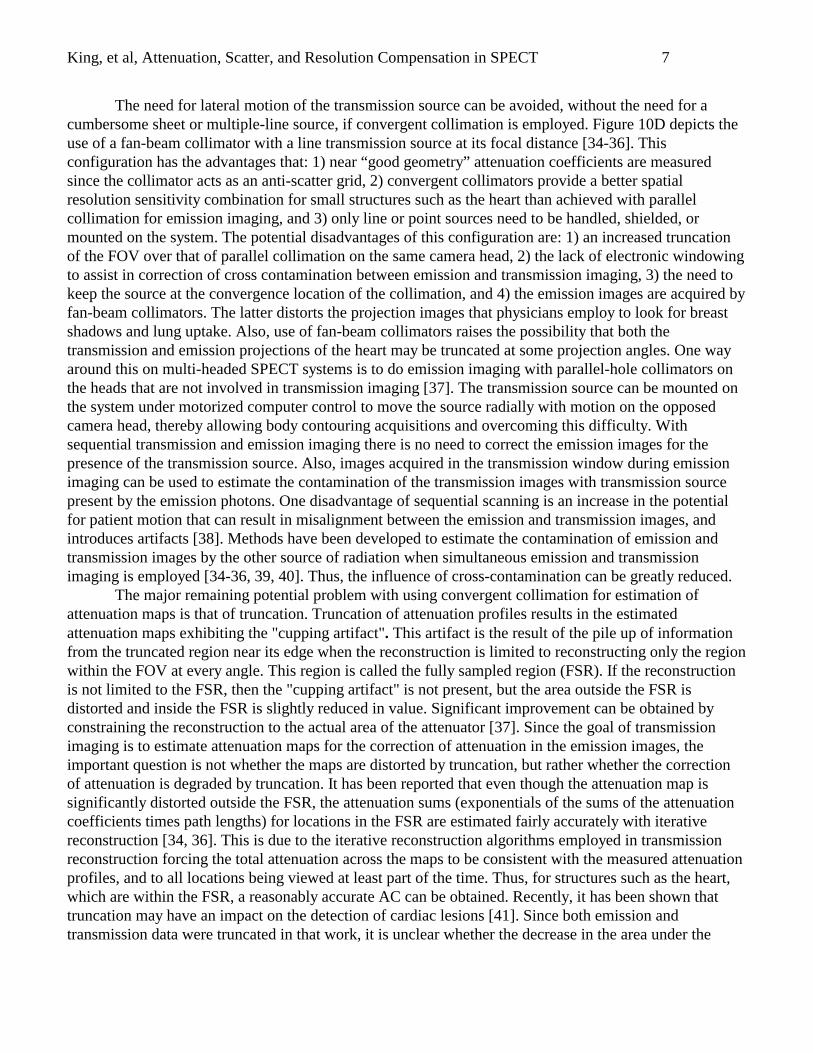
The need for lateral motion of the transmission source can be avoided, without the need for acumbersome sheet or multiple-line source, if convergent collimation is employed. Figure 10D depicts theuse of a fan-beam collimator with a line transmission source at its focal distance [34-36]. Thisconfiguration has the advantages that: 1) near “good geometry” attenuation coefficients are measuredsince the collimator acts as an anti-scatter grid, 2) convergent collimators provide a better spatialresolution sensitivity combination for small structures such as the heart than achieved with parallelcollimation for emission imaging, and 3) only line or point sources need to be handled, shielded, ormounted on the system. The potential disadvantages of this configuration are: 1) an increased truncationof the FOV over that of parallel collimation on the same camera head, 2) the lack of electronic windowingto assist in correction of cross contamination between emission and transmission imaging, 3) the need tokeep the source at the convergence location of the collimation, and 4) the emission images are acquired byfan-beam collimators. The latter distorts the projection images that physicians employ to look for breastshadows and lung uptake. Also, use of fan-beam collimators raises the possibility that both thetransmission and emission projections of the heart may be truncated at some projection angles. One wayaround this on multi-headed SPECT systems is to do emission imaging with parallel-hole collimators onthe heads that are not involved in transmission imaging [37]. The transmission source can be mounted onthe system under motorized computer control to move the source radially with motion on the opposedcamera head, thereby allowing body contouring acquisitions and overcoming this difficulty. Withsequential transmission and emission imaging there is no need to correct the emission images for thepresence of the transmission source. Also, images acquired in the transmission window during emissionimaging can be used to estimate the contamination of the transmission images with transmission sourcepresent by the emission photons. One disadvantage of sequential scanning is an increase in the potentialfor patient motion that can result in misalignment between the emission and transmission images, andintroduces artifacts [38]. Methods have been developed to estimate the contamination of emission andtransmission images by the other source of radiation when simultaneous emission and transmissionimaging is employed [34-36, 39, 40]. Thus, the influence of cross-contamination can be greatly reduced.
The major remaining potential problem with using convergent collimation for estimation ofattenuation maps is that of truncation. Truncation of attenuation profiles results in the estimatedattenuation maps exhibiting the "cupping artifact". This artifact is the result of the pile up of informationfrom the truncated region near its edge when the reconstruction is limited to reconstructing only the regionwithin the FOV at every angle. This region is called the fully sampled region (FSR). If the reconstructionis not limited to the FSR, then the "cupping artifact" is not present, but the area outside the FSR isdistorted and inside the FSR is slightly reduced in value. Significant improvement can be obtained byconstraining the reconstruction to the actual area of the attenuator [37]. Since the goal of transmissionimaging is to estimate attenuation maps for the correction of attenuation in the emission images, theimportant question is not whether the maps are distorted by truncation, but rather whether the correctionof attenuation is degraded by truncation. It has been reported that even though the attenuation map issignificantly distorted outside the FSR, the attenuation sums (exponentials of the sums of the attenuationcoefficients times path lengths) for locations in the FSR are estimated fairly accurately with iterativereconstruction [34, 36]. This is due to the iterative reconstruction algorithms employed in transmissionreconstruction forcing the total attenuation across the maps to be consistent with the measured attenuationprofiles, and to all locations being viewed at least part of the time. Thus, for structures such as the heart,which are within the FSR, a reasonably accurate AC can be obtained. Recently, it has been shown thattruncation may have an impact on the detection of cardiac lesions [41]. Since both emission andtransmission data were truncated in that work, it is unclear whether the decrease in the area under the
King, et al, Attenuation, Scatter, and Resolution Compensation in SPECT 8
ROC curve was caused primarily by one, by the other, or by a combination of both types of truncation.There is no question, however, that truncation poses a serious problem for the AC of structures that areoutside of the FOV at some angles.
Truncation can be eliminated, or at least dramatically reduced, by imaging with an asymmetric asopposed to a symmetric fan-beam collimator [42-45]. As shown in Figure 10E, use of asymmetriccollimation results in one side of the patient being truncated, instead of both. By rotating the collimator3600 around the patient, conjugate views will fill in the region truncated. If a point source with electroniccollimator is employed instead of a line source, then a significant improvement in cross-talk can beobtained [46]. Other benefits are that point sources cost less than line sources, and are easier to shield andcollimate. The problem remains, however, that converging collimators acquire the emission profiles. Thisdifficulty can be overcome, as illustrated in Figure 10F, by using photons from a medium-energyscanning-point source to create an asymmetric fan-beam transmission projection through a parallel-holecollimator by penetrating the septa of the collimator [47]. With this strategy, transmission imaging isperformed sequentially after emission imaging to avoid transmission photons from contaminating theemission data. This lengthens the period of time that the patient must remain motionless on the imagingtable. Another problem with this method of transmission imaging is that it really is only useful forimaging with low-energy parallel-hole collimators. For imaging medium-energy and high-energy photonemitters, an asymmetric fan-beam collimator would need to be employed.
Alternatives to transmission imaging for the estimation of attenuation maps do exist. One methodused with cardiac perfusion imaging is to inject Tc-99m macroaggregated albumin (MAA) after thedelayed images and then reimage the patient. The lung region is obtained by segmentation of the MAAlocalization, and the body outline is obtained either by an external wrap soaked in Tc-99m [48], or bysegmentation of scatter-window images [49]. Assigning attenuation coefficients to the soft tissue and lungregions then forms the attenuation map. This method has the advantage of requiring no modification ofthe SPECT system to perform transmission imaging; however, a second pharmaceutical must beadministered, and additional imaging must be performed. Another method of estimating attenuation mapswithout the use of transmission imaging is to segment the body and lung regions from scatter andphotopeak energy window emission images of the imaging agent itself. This would not require anysignificant alteration or addition to present SPECT systems and imaging protocols beyond thesimultaneous acquisition of a scatter window. Application of this method in patient studies has shown thatapproximate segmentation of the lung can be achieved interactively in many, but not all, patients [50].This lack of robustness has limited its clinical use. The emission data does contain information regardingphoton attenuation, and efforts have been made at extracting information on the attenuation coefficientsdirectly from the emission data. One approach for doing so is to iteratively solve for both the emission andattenuation maps from the emission data [51, 52]. Another approach is to use the consistency conditionsof the attenuated Radon transform to assist in defining an attenuation map that would affect the emissionprojections in the same way as the true attenuation distribution [53].
B. Compensation methods for correction of non-uniform attenuation
Not only has the ability to estimate attenuation maps improved greatly during the last decade, butso has the ability to perform AC once the attenuation maps are known. In part this is due to thetremendous changes in computing power, making computations practical which could only be performedas research exercises ten years ago. It is also due to an improvement in the algorithms used for correctionand the efficiency of their implementations. An example is the development of ordered-subset or block-
King, et al, Attenuation, Scatter, and Resolution Compensation in SPECT 9
iterative algorithms for use with maximum-likelihood reconstruction [54, 55]. Numerous AC algorithmshave been proposed and investigated. For example, considerable effort has been directed towards thedirect analytical solution for attenuation as part of reconstruction. Solutions to the Exponential Radontransform (uniform attenuation within a convex attenuator) have been derived [56-60]. These have beenextended to correction of a convex region of uniform attenuation within a non-uniform attenuator [61-63].Recently the Attenuated Radon transform, in the general case of non-uniform attenuation, has beenanalytically solved [64]. Any comprehensive review of AC algorithms would require a chapter dedicatedsolely to this task. Therefore, we will discuss at length only the two most commonly used AC algorithms:the Chang algorithm [65] used with FBP, and use of AC with the maximum-likelihood expectation-maximization reconstruction algorithm (MLEM) [67, 68]. The reader is referred to other reviews formore details and other algorithms [69-71].
To compare the algorithms we will make use of the 3D mathematical cardiac-torso (MCAT)phantom developed at the University of North Carolina at Chapel Hill [1]. Source and attenuation mapsfrom the MCAT phantom were input to the SIMIND Monte Carlo simulation of gamma camera imaging[72]. SIMIND formed 128 x 128 pixel images for 120 angles about the source maps as imaged by a low-energy high-resolution parallel-hole collimator imaging Tc-99m. The primary and scatter componentswere recorded separately. This allowed the study of scatter-free images, that is images upon which"perfect" scatter compensation (SC) had been performed.
A simulation was made in which only the distance-dependent spatial resolution was simulated.This served as an example of "perfect" AC. Figure 11 shows the transverse slices and polar maps for 1800
and 3600 FBP reconstructions of this simulation. The slices were filtered pre-reconstruction with a 2DButterworth filter of order 5.0 and cutoff frequency of 0.4 cycles/cm (0.125 of sampling frequency), asrecommended for Tc-99m sestamibi rest images [73]. Notice the absence of the artifacts outside the heartin the transverse slices. Also, notice the uniformity of counts in the polar map aside from the band ofincreased counts due to the joining of left ventricle (LV) and right ventricle (RV), and the decrease incounts at the apex. These deviations from uniformity illustrate the impact of the partial-volume effect onthe uniformity of cardiac wall counts. Where the wall is thicker, as with the joining of the RV and LV, theapparent counts will be higher. Where the wall is thinner, as with apical thinning (which was included inthe simulated LV), the apparent counts will be lower. Thus, even with perfect AC and SC, one would notexpect the wall of the LV to be uniform. Note also that there is slightly better uniformity of counts in the3600 reconstruction than the 1800 reconstruction due to less variation in spatial resolution.
Figure 12 shows a transverse slice through the heart and "Bull's-eye" polar map for 1800 and 3600
FBP reconstructions of the slices with no AC when attenuation was included in the simulation. Again, 2DButterworth filtering of order 5.0 and a cutoff frequency of 0.4 cycles/cm were employed. Notice theartifacts outside the heart due to the reconstruction of inconsistent projections, and the variation inintensity of the LV walls. The polar maps in this figure illustrate the fall-off in counts from the apex to thebase due to the increase in attenuation with depth into the body. A decrease in the anterior wall due to thebreast attenuation for 1800 reconstruction is observed. Notice the slightly better uniformity of the 3600
reconstruction due to the reduction in the impact of projection inconsistencies by combining opposingviews. The goal of AC is to return the reconstructed distributions of Figure 12 to those of Figure 11.
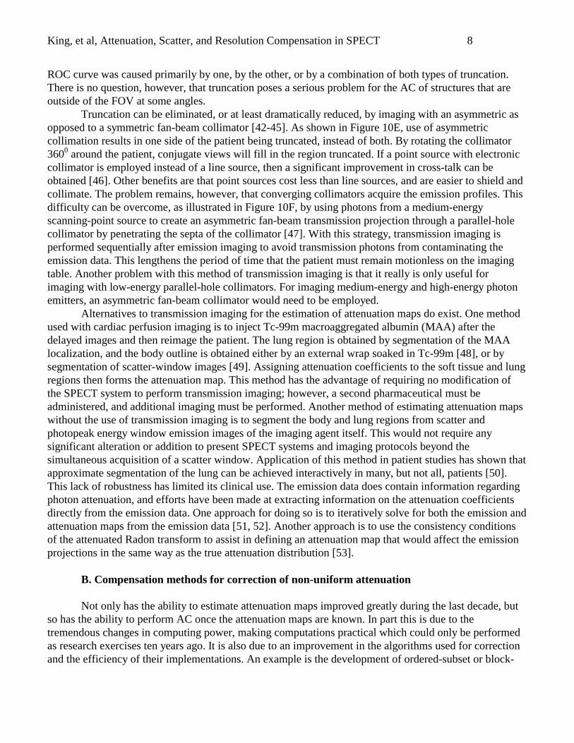
The best known and widest employed of methods that perform AC with FBP is due to Chang [65].The multiplicative or zeroth-order Chang method is a post-reconstruction correction method which seeksto compensate for attenuation by multiplying each point in the body by the reciprocal of the TF, averagedover acquisition angles, from the point to the edge of the body. That is, one calculates the correction factor(C(x', y')) for each (x', y') location in the slice as:
King, et al, Attenuation, Scatter, and Resolution Compensation in SPECT 10
1- M
1 ii ) ,s ,tTF(
M
1 )y ,xC(
′′=′′ ∑
=
θ , (6)
where M is the number of projection angles θi, TF is calculated as per Equation 3, and Equation 1 is usedto convert x' and y' into t' and s' for each θi. The correction is approximate because the TF's are notseparable from the activity when summing over angle [74]. An iterative correction can be obtained in thefollowing way. The zeroth-order corrected slices are projected, mathematically simulating the process ofimaging, and the resulting estimated profiles subtracted from the actual emission data. Error slices arereconstructed from the differences using FBP. After correction of the error slices for attenuation in thesame manner as the zeroth-order correction, the error slices are added to the zeroth-order estimate of theslices to obtain the first-order estimate. Typically only the first-order correction is performed, but theprocess can be repeated any number of times to obtain higher-order estimates. One problem with doingthis is that the method does not converge (i.e., reaches a definite solution and then not changing withfurther iteration). Instead, the higher-order estimates are characterized by elevated noise [75]. Figure 13shows MCAT transverse slices and polar maps for zeroth, first, and fifth-order Chang using the true non-uniform attenuation map to form the correction factors. Notice the considerable improvement of the poorcorrection of zeroth-order Chang after a single iteration. With five iterations, notice the increased noiseevident in the slice and polar map.
As detailed in a previous chapter statistically based reconstruction algorithms start with a modelfor the noise in the emission data and then derive an estimate of the source distribution based on somestatistical criterion. In maximum-likelihood expectation-maximization (MLEM), the noise is modeled asPoisson, and the criterion is to determine the source distribution that most likely gave the emission datausing the expectation-maximization (EM) algorithm [67, 68]. The advantages of MLEM which have leadto its popularity include: 1) it has a good theoretical base; 2) it converges; 3) it readily lends itself to theincorporation of the physics of imaging such as attenuation; and 4) it compensates for non-uniformattenuation with a high degree of accuracy [76].
∑∑∑
=
ik
oldkik
iij
iij
oldjnew
jfh
gh
h
ff
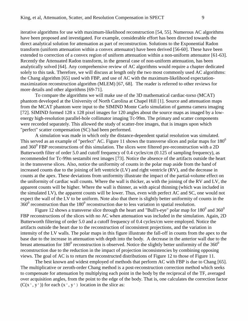
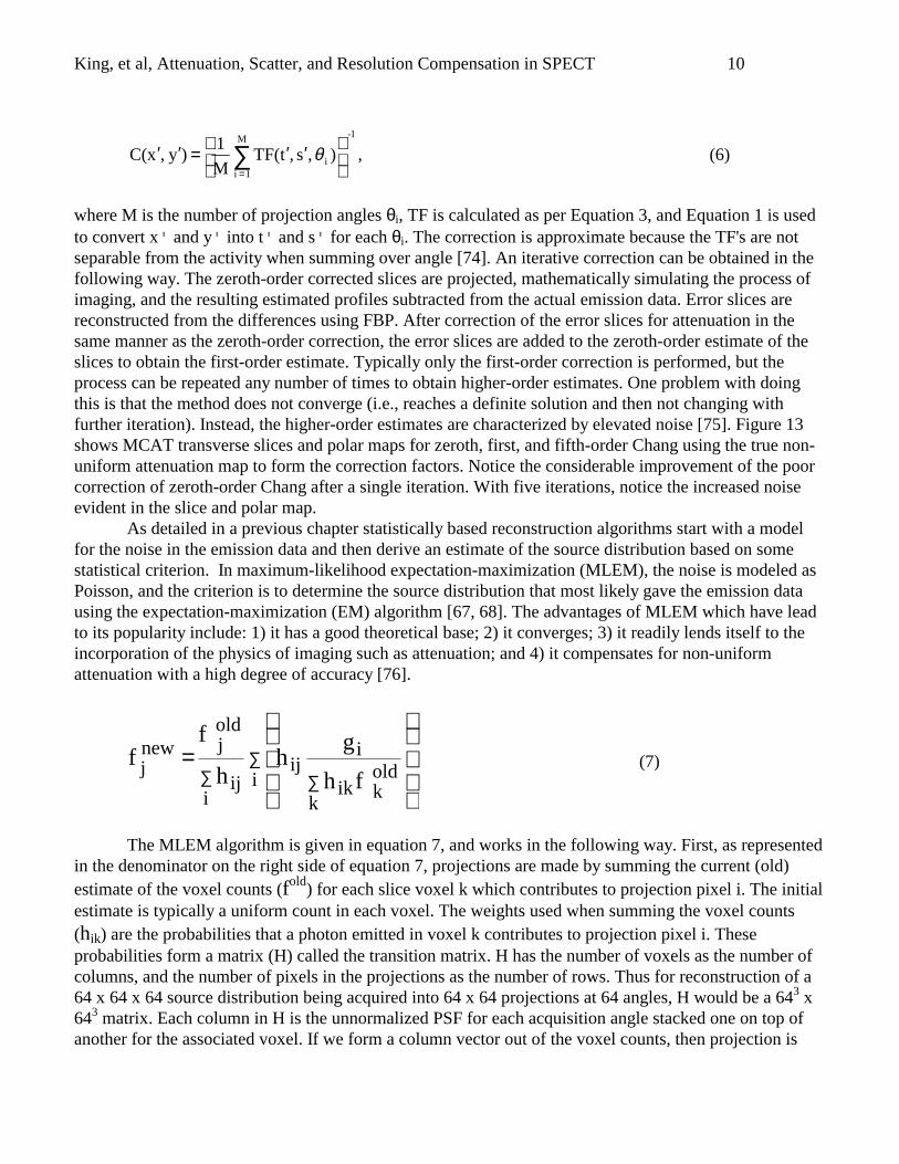
The MLEM algorithm is given in equation 7, and works in the following way. First, as representedin the denominator on the right side of equation 7, projections are made by summing the current (old)estimate of the voxel counts (fold) for each slice voxel k which contributes to projection pixel i. The initialestimate is typically a uniform count in each voxel. The weights used when summing the voxel counts(hik) are the probabilities that a photon emitted in voxel k contributes to projection pixel i. Theseprobabilities form a matrix (H) called the transition matrix. H has the number of voxels as the number ofcolumns, and the number of pixels in the projections as the number of rows. Thus for reconstruction of a64 x 64 x 64 source distribution being acquired into 64 x 64 projections at 64 angles, H would be a 643 x643 matrix. Each column in H is the unnormalized PSF for each acquisition angle stacked one on top ofanother for the associated voxel. If we form a column vector out of the voxel counts, then projection is
(7)
King, et al, Attenuation, Scatter, and Resolution Compensation in SPECT 11
given by the matrix multiplication of H times this vector with the result being a column vector made up ofthe counts in each projection pixel. It is in this process of projecting (mathematically emulating imaging)that one includes the physics of imaging. For example, to include attenuation each hik would be formed asthe product of the TF as calculated by equation 3 times the fractional contribution of voxel k to pixel ibased on the geometry used to model imaging. In reality because of size one would not typically calculateand save the entire H matrix for 3D imaging. Instead, the needed terms are calculated “on-the-fly” by aprocedure such as the following. Projecting along rows or columns is computationally inexpensive.Arbitrary projection angles can be placed in this orientation by appropriately rotating the estimatedemission voxel slices and attenuation maps [77]. Given an aligned attenuation map for an estimate of anemission slice, one could include attenuation by starting with the voxel on the side opposite the projectionbeing created and multiplying its value by the TF for passing through one-half the voxel distance of anattenuator of the given attenuation coefficient. The value of one-half the pixel dimension is usually usedas an approximation for the self-attenuation of the activity in the voxel. One would then move to the nextvoxel along the direction of projection and add its value after correction for self attenuation to the currentprojection sum attenuated by passing through the entire thickness of the voxel. One would then continuethis process until having passed through all voxels along the path of projection. The result of theprojection operation is an estimate of the counts in pixel i based on the current estimate of the voxelcounts, and the model of imaging being used in the transition matrix. As shown by the division on of theright side of equation 7, this estimate is then divided into the actual number of counts acquired in eachpixel i. The ratio of the two indicates if the voxels along the given path of projection are too large (ratiobelow one), just right (ratio of one), or too small (ratio larger than one). These ratios are thenbackprojected as indicated by the summing over i in equation 7, to create an update for the estimate ofvoxel j. This update is the result of letting each ratio vote with a weight of hij on how the current estimateof voxel j should be altered. Note that the summing is now over the first subscript as opposed to thesecond as before. Thus, in terms of matrix algebra, we would be multiplying by the transpose of H in thebackprojection operation. The update is multiplied times the current voxel estimate to obtain the updatedestimate after normalization by dividing by the backprojection of 1.0’s (division just to the right of theequal sign in equation 7).
The ordered-subset version of the MLEM algorithm (OSEM) [54] has accelerated reconstructionto the extent that clinically acceptable reconstruction times are now possible. With OSEM, one divides theprojections into disjoint subsets. One then updates the estimate of the source distribution using just theprojections within the given subset. A single iteration is complete after updating has occurred for all thesubsets. The success of OSEM is such that it is now being used routinely for selected applications insteadof FBP.
Figure 14 shows a comparison of the transverse slices and polar maps in the first column for 30iterations of MLEM using the 1800 of data from RAO to LPO, in the middle column for 30 iterations ofMLEM using all 3600 data, and at the right 100 iterations using all 3600 data. All the reconstructions were3D post-reconstruction filtered with a Butterworth filter with order of 5.0 and cut-off frequency of 0.64cycles/cm. This cut-off is higher than the 0.4 cycles/cm used with all the FBP reconstructions. Notice thatall three yield excellent reconstructions; however, 1800 reconstruction is noisier (especially in the-lowcount areas behind the heart) and the uniformity of the polar map is slightly inferior compared to the 3600
reconstructions. At 100 iterations, the noise has slightly increased, somewhat better resolution is apparentin the transverse slice, and the polar map is a little less uniform than at 30 iterations probably, due to thebetter resolution.
King, et al, Attenuation, Scatter, and Resolution Compensation in SPECT 12
C. Impact of non-uniform attenuation compensation on image quality
AC is required for accurate absolute quantitation of activity [78]. In addition to its alteringquantitation, attenuation is a major cause of artifacts in SPECT slices as discussed earlier. Thus, it is ofinterest to determine if AC can improve diagnostic accuracy in SPECT imaging. An area that has receiveda lot of attention as a candidate for the application of AC is cardiac perfusion imaging. Even though theneed for AC from a physics point of view seems clear, the number of clinical studies reporting negative orequivocal results from the application of AC in perfusion imaging has lead to skepticism concerning itsultimate utility [79, 80]. Two papers do show the potential for improvement in diagnostic accuracy withAC. LaCroix et al. [81] conducted a ROC investigation using the MCAT phantom. They observed animprovement in defect detection when using AC with MLEM as opposed to FBP without AC, particularlyfor simulated patients with large breasts or a raised diaphragm. Ficaro, et al. [82] conducted a ROCinvestigation of AC in 60 patients who had undergone angiography. When coronary artery disease wasdefined as greater than 50 % stenoses in the luminal diameter, the area under the ROC curve increasedfrom 0.734 with no AC to 0.932 with AC. Thus there is reason to believe that ultimately AC will bedetermined to make a significant contribution to improving the diagnostic accuracy of perfusion imaging.Recently a position statement reviewing the literature and summarizing the current view of AC in cardiacimaging has been published [83].
The question of the impact of attenuation and its compensation on tumor-detection accuracy is ofsignificant current clinical interest [84]. Both positive [85] and negative [86] results have been reportedas to the benefit of AC for F-18 labeled 2-fluror-2-deoxy-D-glucose (FDG). Thus, there does not appear tobe a definitive answer yet as to the role of AC in tumor detection for PET FDG imaging.
Using simulated Ga-67 citrate SPECT imaging of the thorax for lymphoma, we [87] performed alocalization receiver operating characteristics (LROC) comparison of: 1) FBP reconstruction with no AC;2) FBP reconstruction with multiplicative Chang AC; 3) FBP with one iteration of iterative Chang AC; 4)one iteration of OSEM with no AC; and 5) one iteration of OSEM with AC. The “free” parameters foreach of the five strategies were optimized using preliminary LROC studies. To compare the strategies,200 lesion sites were randomly selected from a mask of potential lymphoma locations. 100 of these wereused in observer training and strategy optimization, and 100 were used in data collection with 5 physicianobservers. In this study 3 different lesion contrasts were investigated; each image set contained an evendistribution of lesion contrasts. We determined that AC does not significantly alter detection accuracywith FBP reconstruction. However, there was a significant improvement in detection accuracy when ACwas included in OSEM (aggregate areas under the LROC curves (AL) of 0.43, 0.39, 0.41, 0.41, and 0.58for FBP no AC, FBP multiplicative Chang, FBP iterative Chang, OSEM no AC, and OSEM with AC,respectively). There were statistically significant differences between OSEM with AC and the other 4reconstruction strategies for the aggregate, and also for two lower lesion contrasts. Numerically, OSEMwith AC resulted in a larger AL than did the other 4 strategies at the highest contrast considered, but thedifference was no longer statistically significant. We believe this is an indication that once a lesion is ofhigh enough contrast, OSEM with AC no longer provides a significant improvement in performancebecause there is little room for improvement as many of the lesions are obvious to begin with. Wehypothesize that our positive finding for OSEM with AC is due in part to the use of the LROCmethodology with no repetition of lesion locations in the comparison. This prevented the observers frommemorizing the impact of attenuation artifacts on lesion appearance during training. Patient and lesion-site variability would also limit the physician’s ability to do this clinically. Thus we believe that AC mayimprove tumor detection accuracy in SPECT imaging, especially when the tumors are in low-count
King, et al, Attenuation, Scatter, and Resolution Compensation in SPECT 13
regions in slices which also contain significant concentrations of the imaging agent. AC would then helpclean up attenuation artifacts, which spread from the high-count regions and interfere with detection.
III. Scatter Compensation
The imaging of scattered photons degrades contrast and signal-to-noise ratio (SNR), and must beaccounted for if attenuation compensation (AC) is to be accurate [88, 89]. The methods for estimatingattenuation maps available commercially try to estimate “good geometry” attenuation coefficients. In thepast, the use of an effective (reduced) attenuation coefficient approximately accounted for the presence ofscattered as well as primary photons in the projections when performing AC. The coefficient was typicallyselected to under correct the primary content of the emission projections so that a uniform reconstructionof a tub with a uniform concentration of activity resulted when projections with both primary and scatterwere reconstructed [90]. The use of an effective attenuation coefficient to compensate for the presence ofscatter is only, at best, a very approximate solution since the scatter distribution that is detected dependsnot only on the attenuator but also on the source distribution. Patient-activity distributions do notgenerally approximate a tub uniformly filled with activity. Thus instead of using an effective attenuationcoefficient it is better to perform both SC and AC in conjunction since they are a team.
The best way to reduce the effects of scatter would be to improve the energy resolution of theimaging systems by using an alternative to the NaI(Tl) scintillator so that few scattered photons areacquired [5]. Figure 15 shows an energy spectrum obtained using the SIMIND Monte Carlo simulationpackage [72] for an LAO view of the 3D MCAT with the source distribution that of a Tc-99m sestamibiperfusion study as illustrated in Figure 9. Notice the finite width Gaussian response for the primaryphotons due to the finite energy resolution of the system, and the presence of scattered photons under thispeak. The energy resolution (%FWHM) for the NaI(Tl) camera in this simulation was set at 10%. Figure16 shows a plot of how the scatter fraction varies for %FWHM’s of 1% to 10% when a symmetricwindow of width twice that of the %FWHM is employed in imaging. Note that both classical andCompton scattering were included in the simulation. From the plot it is evident that even with 1% energyresolution there would still be a small amount of scatter imaged. Besides improving energy resolution tohave less scatter within the imaging window, one can alter the placement of the energy window over thephotopeak so that it covers less of the region below the peak itself [91]. This reduces the amount of scattercollected, but also reduces the number of primary photons.
A number of SC algorithms have been proposed for SPECT systems that employ NaI(Tl)detectors. Generally, the methods of SC can be divided into two different categories [92, 93]. The firstcategory, which we will call scatter estimation, consists of those methods that estimate the scattercontributions to the projections based on the acquired emission data. The data used may be informationfrom the energy spectrum or a combination of the photopeak data and an approximation of scatter PSF’s.The scatter estimate can be used for SC before, during, or after reconstruction. The second categoryconsists of those methods that model the scatter PSF’s during the reconstruction process. The secondapproach will be called reconstruction-based scatter compensation (RBSC) herein.
A. Scatter estimation methods
The difficulty in scatter estimation is illustrated in Figure 17 which shows that the acquiredprojection data is the result of the contributions from primary photons, scattered photons, and noise. Inscatter estimation one tries to obtain an accurate estimate of the scatter distribution avoiding any biases.
King, et al, Attenuation, Scatter, and Resolution Compensation in SPECT 14
However, even if this is obtained, then its removal from the acquired projection would still leave the noiseinherent in the detection of the scattered photons behind. Thus scatter estimation methods typically reducethe bias in the projections due to scatter, but enhance the noise level.
Energy-distribution-based methods seek to estimate the amount of scatter in a photopeak-energy-window pixel by using the variation of counts acquired, in the same pixel, in one or more energywindows. The pixel-based nature of this method allows for the generation of a scatter estimate for eachpixel in the photopeak-window data. The Compton window subtraction method [94] is the classicexample of this strategy. In this method, a second energy window placed below the photopeak window isused to record a projection consisting of scattered photons. This projection is multiplied by a scalingfactor k, and is then subtracted from the acquired projection to yield a scatter-corrected projection. Thismethod assumes that the spatial distribution of the scatter within the Compton scatter window is the sameas that within the photopeak window, and that once it is determined from a calibration study, a singlescaling factor holds true for all applications on a given system. That the distribution of scatter in the twowindows differs can be seen by noting that the average angle of scattering (and hence the degree ofblurring) changes with energy. Also, the value of k varies depending on radionuclide, energy-windowdefinition, pharmaceutical distribution, region of the body and other factors [95].
Making the scatter window smaller and placing it just below the photopeak window can minimizethe difference in the distribution of scatter between it and the photopeak window. With this arrangement,one obtains the two-energy window variant of the triple-energy window (TEW) SC method [96]. The two-energy window variant is useful when downscatter from a higher energy photon is not present as in thecase of imaging solely Tc-99m. In this method, the scatter in a pixel is estimated as the area under atriangle whose height is the average count per keV in the window below the photopeak window, andwhose base is the width of the photopeak window in keV. When downscatter is present, a third smallwindow is added above the photopeak as illustrated in Figure 18 [97]. With the addition of this thirdwindow, scatter is estimated as the area under the trapezoid formed by the heights of the counts per keV ineach of the two narrow windows on either side of the photopeak, and a base with the width of thephotopeak window. By making the windows smaller, one estimates the scatter distribution from regions ofthe energy spectrum closer to the photopeak window thereby improving the correspondence of thescattered-photon energies with those in the photopeak window. The price paid for this is that theestimation is based on fewer counts and therefore is noisier. Thus heavy low-pass filtering of the scatterestimate is required to reduce the noise in the estimate [98].
Energy-distribution based methods that use a limited number of energy windows to estimate theprimary counts do not completely compensate for scatter. This is in part due to their use of simplegeometric shapes to estimate the scatter within the photopeak window. The main advantages of suchmethods are their speed and simplicity for clinical use. Performance can be improved through the use ofmore windows, which would allow a greater degree of freedom when estimating the scatter within thephotopeak window. A number of investigators have developed multi-window methods [99-101]. Theproblem with methods that require more than a few energy windows is that the required number ofwindows is not available on many SPECT systems. Also, dividing the spectrum up into a large number ofwindows decreases the detected counts in each window, thus increasing the noise in the windows.
Another subclass of scatter-estimation methods is the spatial-distribution-based methods. Thesemethods seek to estimate the scatter contamination of the projections on the basis of the acquiredphotopeak window data, which serves as an estimate of the source distribution, and a model of theblurring of the source into the scatter distribution. The latter is typically an approximation to the scatterPSF, an illustration of which for one location in the 3D MCAT phantom is shown in Figure 19. Beck and
King, et al, Attenuation, Scatter, and Resolution Compensation in SPECT 15
colleagues [102] conducted an early analysis of the contribution of scatter to the response observed forpoint and line sources.
An example of a spatial-distribution method for SC in SPECT is the convolution-subtractionmethod, which modeled the scatter response as decreasing exponentially from its center maximum value[103]. The center value and slope of the exponential were obtained from measurements made with a finitelength line source. This function was convolved with the acquired projection data, and the result was usedas an estimate of the scatter distribution in the projection. The estimated distribution was subtracted fromthe original data to yield scatter corrected projection data. One problem with this method was it assumedthat the scatter model did not change with location. To overcome this problem, Monte Carlo methodswere used to generate a set of scatter responses that were, in turn, used to interpolate the scatter responseat a given location [104]. Both of these approaches used scatter line-spread functions (LSF’s) instead ofPSF’s. That is, the source modeled was a finite length line instead of a point. Convolution was performedone-dimensionally in the plane of the slice to be reconstructed. Scatter originating outside the plane wasassumed to be included as a result of using the finite length line.
Msaki, et al., [105] modeled the two-dimensional (2D) scatter PSF and performed 2D convolutionto account for across-plane scatter as well as in-plane scatter. This method was further refined by adaptingthe scatter PSF for the individual patient using photon transmission through an attenuation map [106,107]. Convolution-subtraction methods offer a fast and reasonably accurate way of correcting for scatter.Their main disadvantages are: the subtraction of the scatter estimate elevates noise in the primaryestimate, the accuracy with which the scatter PSF is modeled is often poor, and the estimation of scatterfrom sources not within the field of view of the camera poses a problem.
B. Reconstruction-based scatter compensation (RBSC) methods
RBSC starts with the estimated source and attenuation distributions and calculates the contributionof scatter to the projections by using the underlying principles of scattering interactions. With RBSCmethods compensation is achieved, in effect, by mapping scattered photons back to their point of origininstead of trying to determine a separate estimate of the scatter contribution to the projections [93]. All ofthe photons are used in RBSC, and it has been argued that there should be less noise increase than withthe other category of compensation [92,93]. One disadvantage, which RBSC shares with the convolution-based subtraction method discussed in the previous section, is that RBSC does not allow for the directcalculation of scatter from sources that are outside of the reconstructed field of view.
The accuracy of RBSC however depends on the accuracy of modeling scatter, and accuratemodeling of scatter is computation intensive. As with AC, the estimation of accurate patient-specificattenuation maps is essential since they are used to form the patient-specific scatter PSF’s. It is also vitalthat inter-slice (3D) as well as intra-slice (2D) SC be performed [108-110]. Thus, for reconstruction of a64 x 64 x 64 source distribution imaged at 64 angles one would need to form a transition matrixconsisting of 644 PSF’s each consisting of 64 x 64 terms, or 64.7 x 10⁹ terms in total. Since each patientpresents a unique attenuation distribution, the transition matrix used in reconstruction ideally should beformed for the individual patient. Such a transition matrix could be obtained by manufacturing anattenuation distribution which matches the patient’s, and in which a point source can be positionedindependently in each voxel to allow measurement of the PSF’s. However, the point source imaging timeis prohibitive for routine clinical use, and the storage in memory and on disk of such a matrix represents asignificant problem even by today’s hardware standards. Thus, the terms in the matrix are normallycalculated as needed without saving them, and with various levels of approximation. Also, the
King, et al, Attenuation, Scatter, and Resolution Compensation in SPECT 16
contribution of scatter to the projections may be calculated directly without the actual formation of thePSF’s as in the case of Monte Carlo simulation.
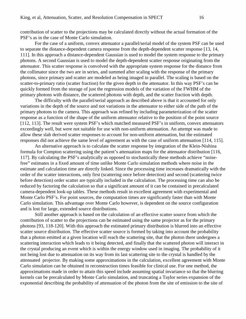
For the case of a uniform, convex attenuator a parallel/serial model of the system PSF can be usedto separate the distance-dependent camera response from the depth-dependent scatter response [13, 14,111]. In this approach a distance-dependent Gaussian is used to model the system response to the primaryphotons. A second Gaussian is used to model the depth-dependent scatter response originating from theattenuator. This scatter response is convolved with the appropriate system response for the distance fromthe collimator since the two are in series, and summed after scaling with the response of the primaryphotons, since primary and scatter are modeled as being imaged in parallel. The scaling is based on thescatter-to-primary ratio (scatter fraction) for the given depth in the attenuator. In this way PSF’s can bequickly formed from the storage of just the regression models of the variation of the FWHM of theprimary photons with distance, the scattered photons with depth, and the scatter fraction with depth.
The difficulty with the parallel/serial approach as described above is that it accounted for onlyvariations in the depth of the source and not variations in the attenuator to either side of the path of theprimary photons to the camera. This approach was refined by including parameterization of the scatterresponse as a function of the shape of the uniform attenuator relative to the position of the point source[112, 113]. The result were system PSF’s which matched measured PSF’s in uniform, convex attenuatorsexceedingly well, but were not suitable for use with non-uniform attenuation. An attempt was made toallow these slab derived scatter responses to account for non-uniform attenuation, but the estimatedresponses did not achieve the same level of agreement as with the case of uniform attenuation [114, 115].
An alternative approach is to calculate the scatter response by integration of the Klein-Nishinaformula for Compton scattering using the patient’s attenuation maps for the attenuator distribution [116,117]. By calculating the PSF’s analytically as opposed to stochastically these methods achieve “noise-free” estimates in a fixed amount of time unlike Monte Carlo simulation methods where noise in theestimate and calculation time are directly linked. Since the processing time increases dramatically with theorder of the scatter interactions, only first (scattering once before detection) and second (scattering twicebefore detection) order scatter are typically included in the calculation. The processing time can also bereduced by factoring the calculation so that a significant amount of it can be contained in precalculatedcamera-dependent look-up tables. These methods result in excellent agreement with experimental andMonte Carlo PSF’s. For point sources, the computation times are significantly faster than with MonteCarlo simulation. This advantage over Monte Carlo however, is dependent on the source configurationand is lost for large, extended source distributions.
Still another approach is based on the calculation of an effective scatter source from which thecontribution of scatter to the projections can be estimated using the same projector as for the primaryphotons [93, 118-120]. With this approach the estimated primary distribution is blurred into an effectivescatter source distribution. The effective scatter source is formed by taking into account the probabilitythat a photon emitted at a given location will reach the scattering site, that the photon there undergoes ascattering interaction which leads to it being detected, and finally that the scattered photon will interact inthe crystal producing an event which is within the energy window used in imaging. The probability of itnot being lost due to attenuation on its way from its last scattering site to the crystal is handled by theattenuated projector. By making some approximations in the calculation, excellent agreement with MonteCarlo simulation can be obtained in reconstruction times feasible for clinical use. For one method, theapproximations made in order to attain this speed include assuming spatial invariance so that the blurringkernels can be precalculated by Monte Carlo simulation, and truncating a Taylor series expansion of theexponential describing the probability of attenuation of the photon from the site of emission to the site of
King, et al, Attenuation, Scatter, and Resolution Compensation in SPECT 17
last scattering [93, 118]. With use of Monte Carlo precalculated kernels, the path of the photon fromemission to last scattering interaction before detection can include scattering interactions up to any orderdesired. However, these intermediate scatterings are assumed to occur in a uniform medium. Analternative method formulates the effective scatter source distribution by incrementally blurring andattenuating each layer of the patient forward towards the detector [119, 120]. The attenuation coefficientsfrom the estimated attenuation map are used to do the layer by layer attenuation, thus this method does notassume a uniform medium when correcting for the attenuation from the site of emission to scattering. Theincremental blurring is however based on a Gaussian approximation to first-order Compton scattering ascalculated from the Klein-Nishina equation. Thus only first-order scatter makes up between 80% and 90%of the scattering events in the Tc-99m photopeak window are included. The effective scatter source imageis created from the result of the incremental blurring and attenuation through multiplication by the voxelattenuation coefficient. This effective scatter source image is then incrementally projected taking intoaccount attenuation and system spatial resolution to produce the estimate of scatter in the projection. Inthis final stage the alteration of the attenuation coefficient resulting from the change in the energy of thephotons upon scattering is not accounted for.
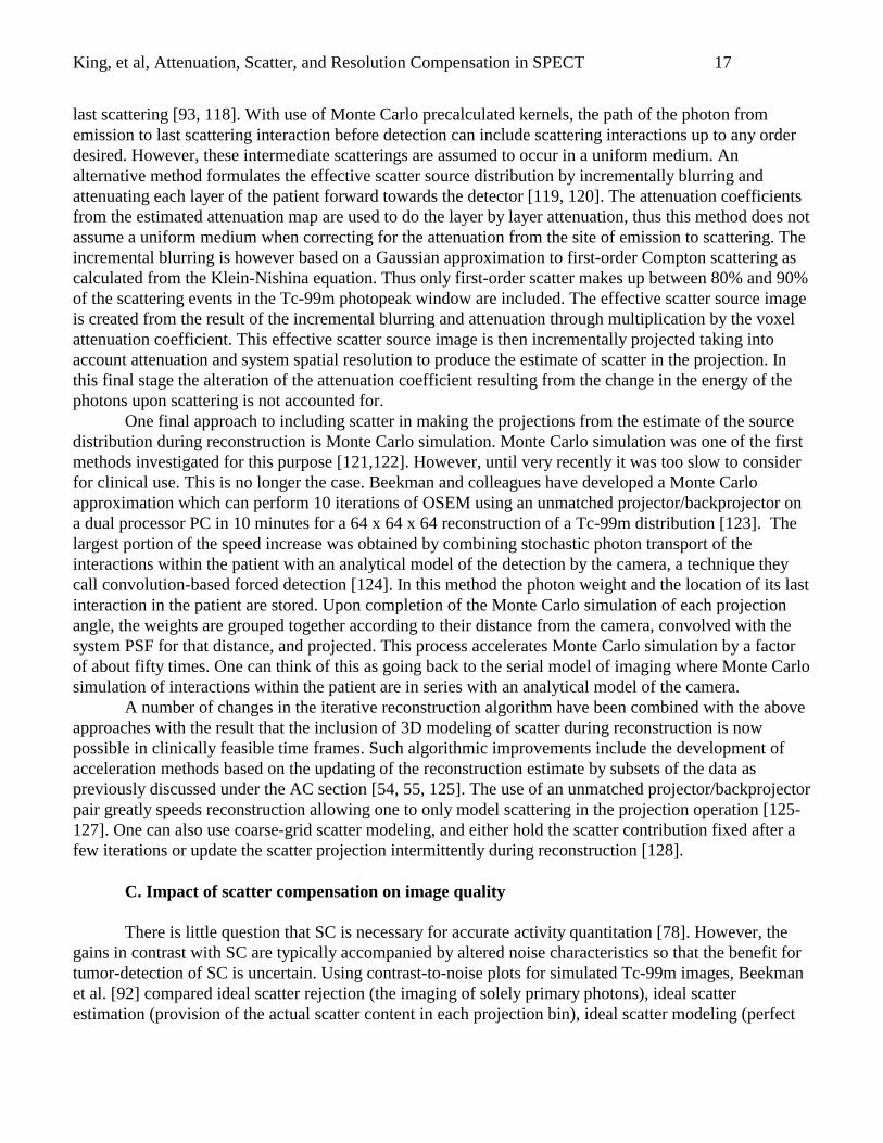
One final approach to including scatter in making the projections from the estimate of the sourcedistribution during reconstruction is Monte Carlo simulation. Monte Carlo simulation was one of the firstmethods investigated for this purpose [121,122]. However, until very recently it was too slow to considerfor clinical use. This is no longer the case. Beekman and colleagues have developed a Monte Carloapproximation which can perform 10 iterations of OSEM using an unmatched projector/backprojector ona dual processor PC in 10 minutes for a 64 x 64 x 64 reconstruction of a Tc-99m distribution [123]. Thelargest portion of the speed increase was obtained by combining stochastic photon transport of theinteractions within the patient with an analytical model of the detection by the camera, a technique theycall convolution-based forced detection [124]. In this method the photon weight and the location of its lastinteraction in the patient are stored. Upon completion of the Monte Carlo simulation of each projectionangle, the weights are grouped together according to their distance from the camera, convolved with thesystem PSF for that distance, and projected. This process accelerates Monte Carlo simulation by a factorof about fifty times. One can think of this as going back to the serial model of imaging where Monte Carlosimulation of interactions within the patient are in series with an analytical model of the camera.
A number of changes in the iterative reconstruction algorithm have been combined with the aboveapproaches with the result that the inclusion of 3D modeling of scatter during reconstruction is nowpossible in clinically feasible time frames. Such algorithmic improvements include the development ofacceleration methods based on the updating of the reconstruction estimate by subsets of the data aspreviously discussed under the AC section [54, 55, 125]. The use of an unmatched projector/backprojectorpair greatly speeds reconstruction allowing one to only model scattering in the projection operation [125-127]. One can also use coarse-grid scatter modeling, and either hold the scatter contribution fixed after afew iterations or update the scatter projection intermittently during reconstruction [128].
C. Impact of scatter compensation on image quality
There is little question that SC is necessary for accurate activity quantitation [78]. However, thegains in contrast with SC are typically accompanied by altered noise characteristics so that the benefit fortumor-detection of SC is uncertain. Using contrast-to-noise plots for simulated Tc-99m images, Beekmanet al. [92] compared ideal scatter rejection (the imaging of solely primary photons), ideal scatterestimation (provision of the actual scatter content in each projection bin), ideal scatter modeling (perfect
King, et al, Attenuation, Scatter, and Resolution Compensation in SPECT 18
knowledge of the scatter PSF’s, which is the ideal for the RBSC methods), and no SC. They determinedthat ideal scatter rejection was the best, followed by ideal scatter modeling, and then ideal scatterestimation. Similar results were reported by Kadrmas et al. [93] for Tl-201 cardiac imaging. They notedthat they had not performed a study of differences in noise correlations between the methods, and that“such differences would be expected to affect the usefulness of reconstructed images for tasks such aslesion detection”.
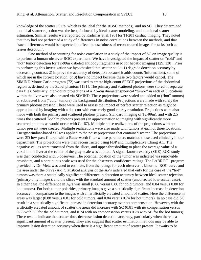
One method of accounting for noise correlation in a study of the impact of SC on image quality isto perform a human-observer ROC experiment. We have investigated the impact of scatter on “cold” and“hot” tumor detection for Tc-99m -labeled antibody fragments used for hepatic imaging [129, 130]. Priorto performing this investigation we hypothesized that scatter could: 1) degrade detection accuracy bydecreasing contrast; 2) improve the accuracy of detection because it adds counts (information), some ofwhich are in the correct location; or 3) have no impact because these two factors would cancel. TheSIMIND Monte Carlo program [72] was used to create high-count SPECT projections of the abdominalregion as defined by the Zubal phantom [131]. The primary and scattered photons were stored in separatedata files. Similarly, high-count projections of a 2.5-cm diameter spherical “tumor” in each of 3 locationswithin the liver were also created via SIMIND. These projections were scaled and added to (“hot” tumors)or subtracted from (“cold” tumors) the background distribution. Projections were made with solely theprimary photons present. These were used to assess the impact of perfect scatter rejection as might beapproximated by imaging with a detector with extremely good energy resolution. Projections were alsomade with both the primary and scattered photons present (standard imaging of Tc-99m), and with 2.5times the scattered Tc-99m photons present (an approximation to imaging with significantly morescattered photons as would occur with Ga-67). Multiple noise realizations of the projections with notumor present were created. Multiple realizations were also made with tumors at each of three locations.Energy-window-based SC was applied to the noisy projections that contained scatter. The projectionswere 2D low-pass filtered with a Butterworth filter whose parameters matched those used clinically in ourdepartment. The projections were then reconstructed using FBP and multiplicative Chang AC. Thenegative values were truncated from the slices, and upper-thresholding to place the average value of avoxel in the liver at the center of the gray-scale was applied. A signal-known-exactly (SKE) ROC studywas then conducted with 5 observers. The potential location of the tumor was indicated via removablecrosshairs, and a continuous scale was used for the observers' confidence ratings. The LABROC1 programprovided by Dr. Metz was used to estimate, from the ratings for each observer, a binormal ROC curve andthe area under the curve (AZ). Statistical analysis of the AZ’s indicated that only for the case of the “hot”tumors was there a statistically significant difference in detection accuracy between ideal scatter rejection(primary-only images), and the slices with the standard amount of scatter (uncorrected low-scatter case).In either case, the difference in AZ’s was small (0.88 versus 0.86 for cold tumors, and 0.84 versus 0.80 forhot tumors). For both tumor polarities, primary images gave a statistically significant increase in detectionaccuracy in comparison to the images with an artificially elevated amount of scatter. Here the difference inareas was larger (0.88 versus 0.81 for cold tumors, and 0.84 versus 0.74 for hot tumors). In no case did SCresult in a statistically significant increase in detection accuracy over no compensation. However, with theartificially elevated amount of scatter the areas did increase with SC (0.81 with no compensation versus0.83 with SC for the cold tumors, and 0.74 with no compensation versus 0.78 with SC for the hot tumors).These results indicate that scatter does decrease lesion detection accuracy, particularly when there is asignificant amount of scatter present. They also suggest that scatter estimation methods may be able toimprove lesion detection accuracy when there is a significant amount of scatter present. It awaits to be
King, et al, Attenuation, Scatter, and Resolution Compensation in SPECT 19
seen whether RBSC methods are superior to estimation methods for undoing the impact of scatter onlesion detection.
IV. Spatial Resolution Compensation
A. Restoration filtering
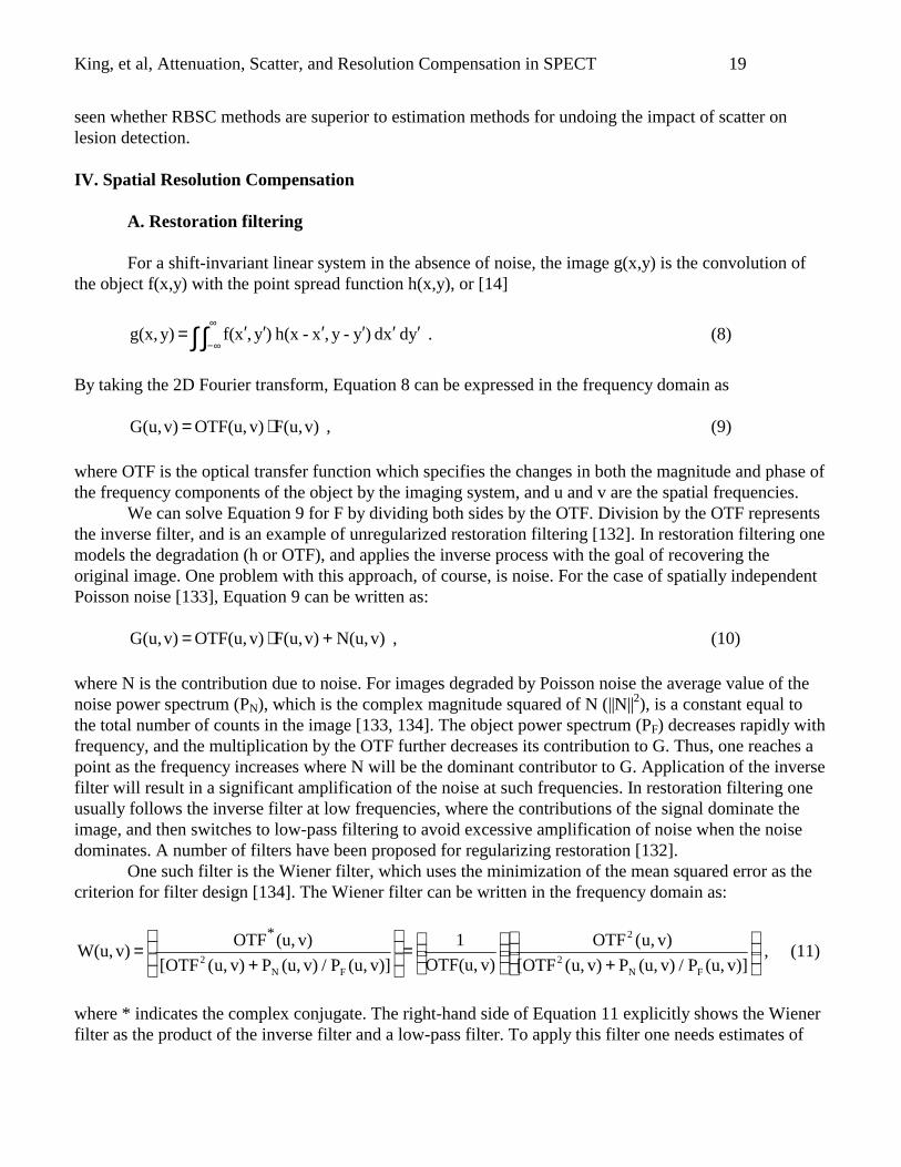
For a shift-invariant linear system in the absence of noise, the image g(x,y) is the convolution ofthe object f(x,y) with the point spread function h(x,y), or [14]
∫ ∫∞
∞−′′′′′′= yd xd )y-y,x-h(x )y,xf( y)g(x, . (8)
By taking the 2D Fourier transform, Equation 8 can be expressed in the frequency domain as
v)F(u, v)OTF(u, v)G(u, ⋅= , (9)
where OTF is the optical transfer function which specifies the changes in both the magnitude and phase ofthe frequency components of the object by the imaging system, and u and v are the spatial frequencies. We can solve Equation 9 for F by dividing both sides by the OTF. Division by the OTF representsthe inverse filter, and is an example of unregularized restoration filtering [132]. In restoration filtering onemodels the degradation (h or OTF), and applies the inverse process with the goal of recovering theoriginal image. One problem with this approach, of course, is noise. For the case of spatially independentPoisson noise [133], Equation 9 can be written as:
v)N(u, v)F(u, v)OTF(u, v)G(u, +⋅= , (10)
where N is the contribution due to noise. For images degraded by Poisson noise the average value of thenoise power spectrum (PN), which is the complex magnitude squared of N (||N||2), is a constant equal tothe total number of counts in the image [133, 134]. The object power spectrum (PF) decreases rapidly withfrequency, and the multiplication by the OTF further decreases its contribution to G. Thus, one reaches apoint as the frequency increases where N will be the dominant contributor to G. Application of the inversefilter will result in a significant amplification of the noise at such frequencies. In restoration filtering oneusually follows the inverse filter at low frequencies, where the contributions of the signal dominate theimage, and then switches to low-pass filtering to avoid excessive amplification of noise when the noisedominates. A number of filters have been proposed for regularizing restoration [132].
One such filter is the Wiener filter, which uses the minimization of the mean squared error as thecriterion for filter design [134]. The Wiener filter can be written in the frequency domain as:
+
=
+=
v)](u,P / v)(u,P v)u,([OTF
v)u,(OTF
v)OTF(u,
1
v)](u,P / v)(u,P v)u,([OTF
v)(u,OTF v)W(u,
FN2
2
FN2
*, (11)
where * indicates the complex conjugate. The right-hand side of Equation 11 explicitly shows the Wienerfilter as the product of the inverse filter and a low-pass filter. To apply this filter one needs estimates of
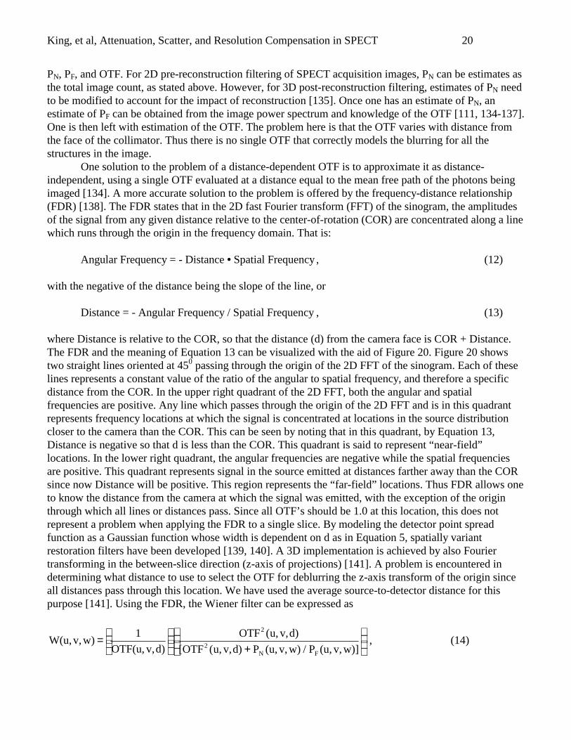
King, et al, Attenuation, Scatter, and Resolution Compensation in SPECT 20
PN, PF, and OTF. For 2D pre-reconstruction filtering of SPECT acquisition images, PN can be estimates asthe total image count, as stated above. However, for 3D post-reconstruction filtering, estimates of PN needto be modified to account for the impact of reconstruction [135]. Once one has an estimate of PN, anestimate of PF can be obtained from the image power spectrum and knowledge of the OTF [111, 134-137].One is then left with estimation of the OTF. The problem here is that the OTF varies with distance fromthe face of the collimator. Thus there is no single OTF that correctly models the blurring for all thestructures in the image.
One solution to the problem of a distance-dependent OTF is to approximate it as distance-independent, using a single OTF evaluated at a distance equal to the mean free path of the photons beingimaged [134]. A more accurate solution to the problem is offered by the frequency-distance relationship(FDR) [138]. The FDR states that in the 2D fast Fourier transform (FFT) of the sinogram, the amplitudesof the signal from any given distance relative to the center-of-rotation (COR) are concentrated along a linewhich runs through the origin in the frequency domain. That is:
Angular Frequency = - Distance • Spatial Frequency , (12)
with the negative of the distance being the slope of the line, or
Distance = - Angular Frequency / Spatial Frequency , (13)
where Distance is relative to the COR, so that the distance (d) from the camera face is COR + Distance.The FDR and the meaning of Equation 13 can be visualized with the aid of Figure 20. Figure 20 showstwo straight lines oriented at 450 passing through the origin of the 2D FFT of the sinogram. Each of theselines represents a constant value of the ratio of the angular to spatial frequency, and therefore a specificdistance from the COR. In the upper right quadrant of the 2D FFT, both the angular and spatialfrequencies are positive. Any line which passes through the origin of the 2D FFT and is in this quadrantrepresents frequency locations at which the signal is concentrated at locations in the source distributioncloser to the camera than the COR. This can be seen by noting that in this quadrant, by Equation 13,Distance is negative so that d is less than the COR. This quadrant is said to represent “near-field”locations. In the lower right quadrant, the angular frequencies are negative while the spatial frequenciesare positive. This quadrant represents signal in the source emitted at distances farther away than the CORsince now Distance will be positive. This region represents the “far-field” locations. Thus FDR allows oneto know the distance from the camera at which the signal was emitted, with the exception of the originthrough which all lines or distances pass. Since all OTF’s should be 1.0 at this location, this does notrepresent a problem when applying the FDR to a single slice. By modeling the detector point spreadfunction as a Gaussian function whose width is dependent on d as in Equation 5, spatially variantrestoration filters have been developed [139, 140]. A 3D implementation is achieved by also Fouriertransforming in the between-slice direction (z-axis of projections) [141]. A problem is encountered indetermining what distance to use to select the OTF for deblurring the z-axis transform of the origin sinceall distances pass through this location. We have used the average source-to-detector distance for thispurpose [141]. Using the FDR, the Wiener filter can be expressed as
+
=
w)]v,(u,P / w)v,(u,P d)v,u,([OTF
d)v,u,(OTF
d)v,OTF(u,
1 w)v,W(u,
FN2
2
, (14)
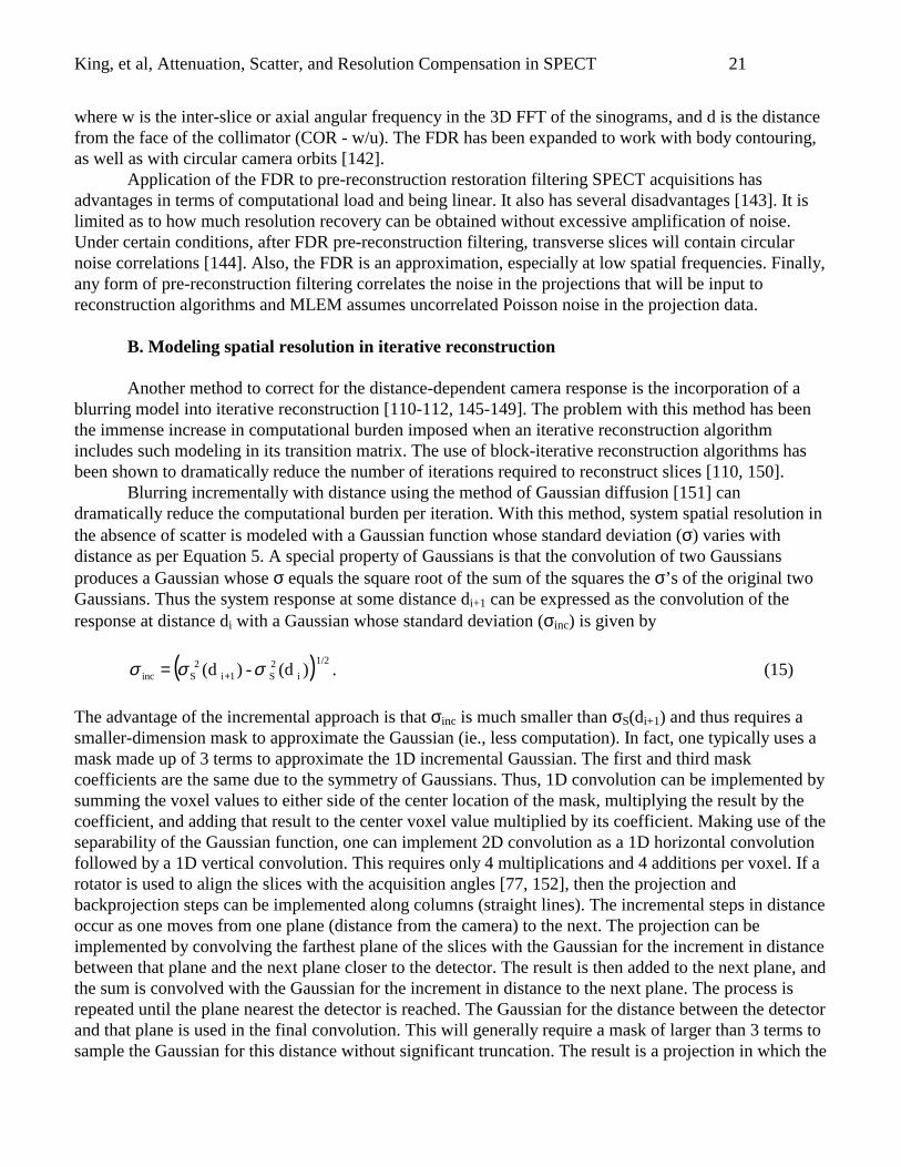
King, et al, Attenuation, Scatter, and Resolution Compensation in SPECT 21
where w is the inter-slice or axial angular frequency in the 3D FFT of the sinograms, and d is the distancefrom the face of the collimator (COR - w/u). The FDR has been expanded to work with body contouring,as well as with circular camera orbits [142].
Application of the FDR to pre-reconstruction restoration filtering SPECT acquisitions hasadvantages in terms of computational load and being linear. It also has several disadvantages [143]. It islimited as to how much resolution recovery can be obtained without excessive amplification of noise.Under certain conditions, after FDR pre-reconstruction filtering, transverse slices will contain circularnoise correlations [144]. Also, the FDR is an approximation, especially at low spatial frequencies. Finally,any form of pre-reconstruction filtering correlates the noise in the projections that will be input toreconstruction algorithms and MLEM assumes uncorrelated Poisson noise in the projection data.
B. Modeling spatial resolution in iterative reconstruction
Another method to correct for the distance-dependent camera response is the incorporation of ablurring model into iterative reconstruction [110-112, 145-149]. The problem with this method has beenthe immense increase in computational burden imposed when an iterative reconstruction algorithmincludes such modeling in its transition matrix. The use of block-iterative reconstruction algorithms hasbeen shown to dramatically reduce the number of iterations required to reconstruct slices [110, 150].
Blurring incrementally with distance using the method of Gaussian diffusion [151] candramatically reduce the computational burden per iteration. With this method, system spatial resolution inthe absence of scatter is modeled with a Gaussian function whose standard deviation (σ) varies withdistance as per Equation 5. A special property of Gaussians is that the convolution of two Gaussiansproduces a Gaussian whose σ equals the square root of the sum of the squares the σ’s of the original twoGaussians. Thus the system response at some distance di+1 can be expressed as the convolution of theresponse at distance di with a Gaussian whose standard deviation (σinc) is given by
( )1/2
i 2 S 1i
2 Sinc )(d - )d( σσσ += . (15)
The advantage of the incremental approach is that σinc is much smaller than σS(di+1) and thus requires asmaller-dimension mask to approximate the Gaussian (ie., less computation). In fact, one typically uses amask made up of 3 terms to approximate the 1D incremental Gaussian. The first and third maskcoefficients are the same due to the symmetry of Gaussians. Thus, 1D convolution can be implemented bysumming the voxel values to either side of the center location of the mask, multiplying the result by thecoefficient, and adding that result to the center voxel value multiplied by its coefficient. Making use of theseparability of the Gaussian function, one can implement 2D convolution as a 1D horizontal convolutionfollowed by a 1D vertical convolution. This requires only 4 multiplications and 4 additions per voxel. If arotator is used to align the slices with the acquisition angles [77, 152], then the projection andbackprojection steps can be implemented along columns (straight lines). The incremental steps in distanceoccur as one moves from one plane (distance from the camera) to the next. The projection can beimplemented by convolving the farthest plane of the slices with the Gaussian for the increment in distancebetween that plane and the next plane closer to the detector. The result is then added to the next plane, andthe sum is convolved with the Gaussian for the increment in distance to the next plane. The process isrepeated until the plane nearest the detector is reached. The Gaussian for the distance between the detectorand that plane is used in the final convolution. This will generally require a mask of larger than 3 terms tosample the Gaussian for this distance without significant truncation. The result is a projection in which the
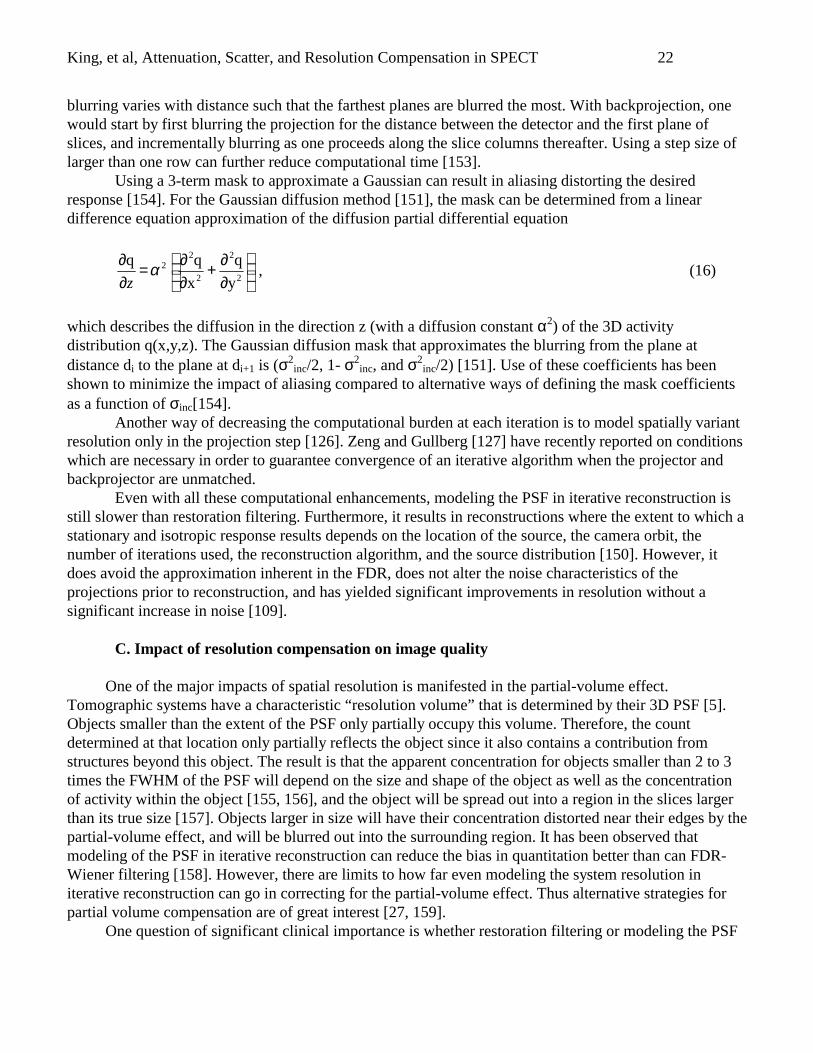
King, et al, Attenuation, Scatter, and Resolution Compensation in SPECT 22
blurring varies with distance such that the farthest planes are blurred the most. With backprojection, onewould start by first blurring the projection for the distance between the detector and the first plane ofslices, and incrementally blurring as one proceeds along the slice columns thereafter. Using a step size oflarger than one row can further reduce computational time [153].
Using a 3-term mask to approximate a Gaussian can result in aliasing distorting the desiredresponse [154]. For the Gaussian diffusion method [151], the mask can be determined from a lineardifference equation approximation of the diffusion partial differential equation
∂∂+
∂∂=
∂∂
2
2
2
22
y
q
x
q
q αz
, (16)
which describes the diffusion in the direction z (with a diffusion constant α2) of the 3D activitydistribution q(x,y,z). The Gaussian diffusion mask that approximates the blurring from the plane atdistance di to the plane at di+1 is (σ2
inc/2, 1- σ2inc, and σ2
inc/2) [151]. Use of these coefficients has beenshown to minimize the impact of aliasing compared to alternative ways of defining the mask coefficientsas a function of σinc[154].
Another way of decreasing the computational burden at each iteration is to model spatially variantresolution only in the projection step [126]. Zeng and Gullberg [127] have recently reported on conditionswhich are necessary in order to guarantee convergence of an iterative algorithm when the projector andbackprojector are unmatched.
Even with all these computational enhancements, modeling the PSF in iterative reconstruction isstill slower than restoration filtering. Furthermore, it results in reconstructions where the extent to which astationary and isotropic response results depends on the location of the source, the camera orbit, thenumber of iterations used, the reconstruction algorithm, and the source distribution [150]. However, itdoes avoid the approximation inherent in the FDR, does not alter the noise characteristics of theprojections prior to reconstruction, and has yielded significant improvements in resolution without asignificant increase in noise [109].
C. Impact of resolution compensation on image quality
One of the major impacts of spatial resolution is manifested in the partial-volume effect.Tomographic systems have a characteristic “resolution volume” that is determined by their 3D PSF [5].Objects smaller than the extent of the PSF only partially occupy this volume. Therefore, the countdetermined at that location only partially reflects the object since it also contains a contribution fromstructures beyond this object. The result is that the apparent concentration for objects smaller than 2 to 3times the FWHM of the PSF will depend on the size and shape of the object as well as the concentrationof activity within the object [155, 156], and the object will be spread out into a region in the slices largerthan its true size [157]. Objects larger in size will have their concentration distorted near their edges by thepartial-volume effect, and will be blurred out into the surrounding region. It has been observed thatmodeling of the PSF in iterative reconstruction can reduce the bias in quantitation better than can FDR-Wiener filtering [158]. However, there are limits to how far even modeling the system resolution initerative reconstruction can go in correcting for the partial-volume effect. Thus alternative strategies forpartial volume compensation are of great interest [27, 159].
One question of significant clinical importance is whether restoration filtering or modeling the PSF
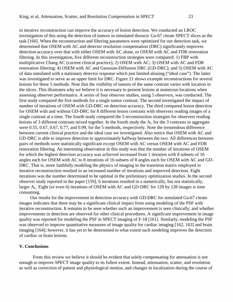
King, et al, Attenuation, Scatter, and Resolution Compensation in SPECT 23
in iterative reconstruction can improve the accuracy of lesion detection. We conducted an LROCinvestigation of this using the detection of tumors in simulated thoracic Ga-67 citrate SPECT slices as thetask [160]. When the reconstruction and filtering parameters were optimized for our detection task, wedetermined that OSEM with AC and detector resolution compensation (DRC) significantly improvesdetection accuracy over that with either OSEM with AC alone, or OSEM with AC and FDR restorationfiltering. In this investigation, five different reconstruction strategies were compared: 1) FBP withmultiplicative Chang AC (current clinical practice); 2) OSEM with AC; 3) OSEM with AC and FDRrestoration filtering; 4) OSEM with AC and Gaussian-Diffusion DRC (GD-DRC); and 5) OSEM with ACof data simulated with a stationary detector response which just limited aliasing (“ideal case”). The latterwas investigated to serve as an upper limit for DRC. Figure 21 shows example reconstructions for severallesions for these 5 methods. Note that the visibility of tumors of the same contrast varies with location inthe slices. This illustrates why we believe it is necessary to present lesions at numerous locations whenassessing observer performance. A series of four observer studies, using 5 observers, was conducted. Thefirst study compared the five methods for a single tumor contrast. The second investigated the impact ofnumber of iterations of OSEM with GD-DRC on detection accuracy. The third compared lesion detectionfor OSEM with and without GD-DRC for 8 different lesion contrasts with observers reading images of asingle contrast at a time. The fourth study compared the 5 reconstruction strategies for observers readinglesions of 3 different contrasts mixed together. In the fourth study the AL for the 3 contrasts in aggregatewere 0.55, 0.67, 0.67, 0.77, and 0.99, for the 5 methods, respectively. Note the tremendous differencebetween current clinical practice and the ideal case we investigated. Also notice that OSEM with AC andGD-DRC is able to improve detection to approximately halfway between the two. All differences betweenpairs of methods were statistically significant except OSEM with AC versus OSEM with AC and FDRrestoration filtering. An interesting observation in this study was that the number of iterations of OSEMfor which the highest detection accuracy was achieved increased from 1 iteration with 8 subsets of 16angles each for OSEM with AC to 8 iterations of 16 subsets of 8 angles each for OSEM with AC and GD-DRC. That is, more faithfully modeling the physics of imaging in the transition matrix employed initerative reconstruction resulted in an increased number of iterations and improved detection. Eightiterations was the number determined to be optimal in the preliminary optimization studies. In the secondobserver study reported in the paper [159], 6 iterations resulted in a numerically, but not statistically,larger AL. Eight (or even 6) iterations of OSEM with AC and GD-DRC for 128 by 128 images is timeconsuming.
Our results for the improvement in detection accuracy with GD-DRC for simulated Ga-67 citrateimages indicates that there may be a significant clinical impact from using modeling of the PSF withiterative reconstruction. It remains to be seen whether such an improvement is seen clinically, and whetherimprovements in detection are observed for other clinical procedures. A significant improvement in imagequality was reported for modeling the PSF in SPECT imaging of F-18 [161]. Similarly, modeling the PSFwas observed to improve quantitative measures of image quality for cardiac imaging [162, 163] and brainimaging [164]; however, it has yet to be determined to what extent such modeling improves the detectionof cardiac or brain lesions.
V. Conclusions
From this review we believe it should be evident that solely compensating for attenuation is notenough to improve SPECT image quality to its fullest extent. Instead, attenuation, scatter, and resolutionas well as correction of patient and physiological motion, and changes in localization during the course of
King, et al, Attenuation, Scatter, and Resolution Compensation in SPECT 24
acquisition can impact image quality, and thus combined compensation is required. It is our opinion thatas a result of improvements in algorithms and computer hardware, the best way to perform suchcompensations is to accurately model the degradations in iterative reconstruction. Evidence is beginningto be obtained that these compensations do significantly improve the diagnostic utility of SPECT images.For example, in an ROC study of the accuracy of detection of coronary disease using cardiac-perfusionSPECT imaging with clinical images, we have recently determined that combined correction forattenuation, scatter, and spatial resolution is more accurate than FBP or solely AC, or AC and SC [165].However, it should be remembered that the corrected images look different than the uncorrected imagesphysicians have grown accustomed to reading. Thus it will require a period of adjustment for theclinicians to develop a new mental picture of what “normal” looks like before the full potential of thecompensations is realized clinically [79, 166].
VI. Acknowledgments
The authors would like to thank the reviewer for suggesting additional material to be added to thischapter. This work was supported in part by US Public Health grants HL50349 and CA42165 of theNational Heart, Lung, and Blood Institute, and National Cancer Institute. Its contents are solely theresponsibility of the authors and do not necessarily represent the official views of the National Heart,Lung, and Blood Institute, or the National Cancer Institute.
VII. References
1. Tsui BMW, Zhao XD, Gregoriou, Lalush DS, Frey EC, Johnston RE, McCartney WH. Quantitativecardiac SPECT reconstruction with reduced image degradation due to patient anatomy. IEEE Trans NuclSci 41: 2838-2848, 1994.
2. Boas ML. Mathematical Methods in the Physical Sciences. Second Edition, John Wiley & Sons, NewYork, 1983.
3. Kak AC, Slaney M. Principles of Computerized Tomographic Imaging. IEEE Press, New York, 1987.
4. Attix FH. Introduction to Radiological Physics and Radiation Dosimetry. John Wiley & Sons, NewYork, 1983.
5. Sorenson JA, Phelps ME. Physics in Nuclear Medicine. Second Edition, Grune & Stratton, Orlando,1987.
6. de Vries DJ, King MA. Window selection for dual photopeak window scatter correction in Tc-99mimaging. IEEE Trans Nucl Sci 41:2771-2778, 1994.
7. Hademenous GJ, King MA, Ljungberg M, Zubal G, Harrell CR. A scatter correction method for Tl-201images: a Monte Carlo investigation. IEEE Trans Nucl Sci 30:1179-1186, 1993.
8. Metz CE, Atkins FB, Beck RN: The geometrical transfer function component for scintillation cameracollimators with straight parallel holes. Phys Med Biol 25: 1059-1070, 1980.
King, et al, Attenuation, Scatter, and Resolution Compensation in SPECT 25
9. Tsui BMW, Gullberg GT. The geometric transfer function for cone and fan beam collimators. PhysMed Biol 35: 81-93, 1990.
10. Frey EC, Tsui BMW, Gullberg GT. Improved estimation of the detector response function forconverging beam collimators. Phys Med Biol 43: 941-950, 1998.
11. Formiconi AR. Geometrical response of multihole collimators. Phys Med Biol 43: 3359-3379, 1998.
12. Brookeman VA, Bauer TJ. Collimator performance for scintillation camera systems. JNM 14: 21-25,1973.
13. Gilland DR, Tsui BMW, McCarthy WH, Perry JR, Berg J. Determination of the optimum filterfunction for SPECT imaging. JNM 29: 643-650, 1988.
14. Metz CE, Doi K: Transfer function analysis of radiographic imaging. Phys Med Biol 24: 1079-1106,1979.
15. Manglos SH, Jaszczak RJ, Floyd CE, Hahn LJ, Greer KL, Coleman RE. A quantitative comparison ofattenuation-weighted backprojection with multiplicative and iterative postprocessing attenuationcompensation in SPECT. IEEE Trans Med Imag 7:128-134, 1988.
16. King MK, Xia W, de Vries DJ, Pan T-S, Villegas BJ, Dahlberg S, Tsui BMW, Ljungberg MH,Morgan HT. A Monte Carlo investigation of artifacts caused by liver uptake in single-photon emissioncomputed tomography perfusion imaging with Tc-99m labeled agents. J Nucl Card 3:18-29, 1996.
17. Germano G, Chua T, Kiat H, Areeda JS, Berman DS. A quantitative phantom analysis of artifacts dueto hepatic activity in technetium-99m myocardial perfusion SPECT studies. J Nucl Med 35:356-359,1994.
18. O’Connor MK, Kelly BJ. Evaluation of techniques for the elimination of “hot” bladder artifacts inSPECT of the pelvis. J Nucl Med 31: 1872-75, 1990.
19. Gillen GJ, Gilmore B, Elliott AT. An investigation of the magnitude and causes of count loss artifactsin SPECT imaging. JNM 32: 1771-1776, 1991.
20. Nuyts J, Dupont P, Van den Maegdenbergh V, Vleugels S, Suetens P, Mortelmans L. A study of liver-heart artifact in emission tomography. J Nucl Med 36:133-139, 1995.
21. Jaszczak RJ, Chang LT, Stein NA, Moore FE. Whole-body single-photon emission computedtomography using dual, large-field-of-view scintillation cameras. Phys Med Biol 24:1123-1143, 1979.
22. King MA, Tsui BMW, Pan T-S. Attenuation compensation for cardiac single-photon emissioncomputed tomographic imaging: Part 1. Impact of attenuation and methods of estimating attenuationmaps. J Nucl Card 2:513-524, 1995.
King, et al, Attenuation, Scatter, and Resolution Compensation in SPECT 26
23. Fleming JS. A technique for using CT images in attenuation correction and quantification in SPECT.Nucl Med Comm 10:83-97, 1989.
24. Meyer CR, Boes JL, Kim B, Bland PH, Zasadny KR, Kison PV, Koral K, Frey KA, Wahl RL.Demonstration of accuracy and clinical versatility of mutual information for automatic multimodalityimage fusion using affine and thin-plate spline warped geometric deformations. Med Imag Anal 1:195-206, 1996.
25. Blankespoor SC, Wu X, Kalki K, Brown JK, Tang HR, Cann CE, Hasegawa BH. Attenuationcorrection of SPECT using x-ray CT on an emission-transmission CT system: myocardial perfusionassessment. IEEE Trans Nucl Sci 43:2263-2274, 1996.
26. LaCroix KJ, Tsui BMW, Hasegawa BH, Brown JK. Investigation of the use of x-ray CT images forattenuation compensation in SPECT. IEEE Trans Nucl Sci 41:2793-2799, 1994.
27. Da Silva AJ, Tang HR, Wong KH, Wu MC, Dae MW, Hasegawa BH. Absolute quantification ofregional myocardial uptake of Tc-99m- sestamibi with SPECT: experimental validation in a porcinemodel. J Nucl Med 42:772-779, 2001.
28. Maeda H, Itoh H, Ishii Y, Makai T, Todo G, Fujita T, Torizuka K. Determination of the pleural edgeby gamma-ray transmission computed tomography. JNM 22:815-817, 1981
29. Malko JA, Van Heertum RL, Gullberg GT, Kowalsky WP. SPECT liver imaging using an iterativeattenuation correction algorithm and an external flood source. JNM 26:701-705, 1985.
30. Bailey DL, Hutton BF, Walker PJ. Improved SPECT using simultaneous emission and transmissiontomography. JNM 28:844-851, 1987.
31. Cao ZJ, Tsui BMW. Performance characteristics of transmission imaging using a uniform sheet sourcewith a parallel-hole collimator. Med Phys 19:1205-1212, 1992.
32. Celler A, Sitek A, Stoub E, Hawman P, Harrop R, Lyster D. Multiple line source array for SPECTtransmission scans: simulation, phantom, and patient studies. JNM 39:2183-2189, 1998.
33. Tan P, Bailey DL, Meikle SR, Eberl S, Fulton RR, Hutton BF. A scanning line source forsimultaneous emission and transmission measurements in SPECT. JNM 34:1752-1760, 1993.
34. Tung C-H, Gullberg GT, Zeng GL, Christian PE, Datz FL, Morgan HT. Nonuniform attenuationcorrection using simultaneous transmission and emission converging tomography. IEEE Trans Nucl Sci39:1134-1143, 1992.
35. Jaszczak RJ, Gilland DR, Hanson MW, Jang S, Greer KL, Coleman RE. Fast transmission CT fordetermining attenuation maps using a collimated line source, rotatable air-copper-lead attenuators and fan-beam collimation. JNM 34:1577-1586, 1993.
King, et al, Attenuation, Scatter, and Resolution Compensation in SPECT 27
36. Gullberg GT, Morgan HT, Zeng GL, Christian PE, Di Bella EVR, Tung C-H, Maniawski PJ, Hsieh Y-L, Datz FL. The design and performance of a simultaneous transmission and emission tomographysystem. IEEE Trans Nucl Sci 45:1676-1698, 1998.
37. Narayanan MV, King MA, Pan T-S, Dahlberg ST. Investigation of approaches to reduce truncation ofattenuation maps with simultaneous transmission and emission SPECT imaging. IEEE Trans Nucl Sci45:1200-1206, 1998.
38. Stone CD, McCormick JW, Gilland DR, Greer KL, Coleman RE, Jaszczak RJ. Effect of registrationerrors between transmission and emission scans on a SPECT system using sequential scanning. JNM39:365-373, 1998.
39. Barnden LR, Ong PL, Rowe CC. Simultaneous emission transmission tomography using technetium-99m for both emission and transmission. EJNM 24:1390-1397, 1997.
40. Narayanan MV, King MA, Byrne CL. An iterative transmission algorithm incorporating cross-talkcorrection for SPECT. Med Phys 29:694-700, 2002.
41. Gregoriou GK, Tsui BMW, Gullberg GT. Effect of truncated projections on defect detection inattenuation-compensated fanbeam cardiac SPECT. JNM 39:166-175, 1998.
42. Chang W, Loncaric S, Huang G, Sanpitak P. Asymmetric fan transmission CT on SPECT systems.Phys Med Biol 40:913-928, 1995.
43. Gilland DR, Jaszczak RJ, Greer KL, Coleman RE. Transmission imaging for nonuniform attenuationcorrection using a three-headed SPECT camera. JNM 39:1005-1110, 1998.
44. Hollinger EF, Loncaric S, Yu D-C, Ali A, Chang W. Using fast sequential asymmetric fanbeamtransmission CT for attenuation correction of cardiac SPECT imaging. JNM 1335-1344, 1998.
45. LaCroix KJ, Tsui BMW. Investigation of 90 dual-camera half-fanbeam collimation for myocardialSPECT imaging. IEEE Trans Nucl Sci 46:2085-2092, 1999.
46. Beekman FJ, Kamphuis C, Hutton BF, van Rijk PP. Half-fanbeam collimators combined withscanning point sources for simultaneous emission-transmission imaging. JNM 39:1996-2003, 1998.
47. Gagnon D, Tung CH, Zeng L, Hawkins WG. Design and early testing of a new medium-energytransmission device for attenuation correction in SPECT and PET. Proceed 1999 Med Imag Conf, IEEE,2000, Paper M8-3.
48. Madsen MT, Kirchner PT, Edlin JP, Nathan MA, Kahn D. An emission-based technique for obtainingattenuation correction data for myocardial SPECT studies. Nucl Med Comm 14:689-695, 1993.
King, et al, Attenuation, Scatter, and Resolution Compensation in SPECT 28
49. Wallis JW, Miller TR, Koppel P. Attenuation correction in cardiac SPECT without a transmissionmeasurement. JNM 36:506-512, 1995.
50. Pan T-S, King MA, Luo D-S, Dahlberg ST, Villegas BJ. Estimation of attenuation maps from scatterand photopeak window single photon emission computed tomographic images of technetium-99m labeledsestamibi. J Nucl Card 4:42-51, 1997.
51. Manglos SH, Young TM. Constrained IntraSPECT reconstruction from SPECT projections. Proceed1993 MIC. 1605-1609, 1994.
52. Nuyts J, Dupont P, Stroobans S, Benninck R, Mortelmans L, Suetens P. Simultaneous maximum aposteriori reconstruction of attenuation and activity distributions from emission sinograms. IEEE TransMed Imag 18:393-403, 1999.
53. Welch A, Clack R, Natterer F, Gullberg GT. Toward accurate attenuation correction in SPECTwithout transmission measurements. IEEE Trans Med Imag 16:532-541, 1997.
54. Hudson HM, Larkin RS. Accelerated image reconstruction using ordered subsets of projection data.IEEE Trans Med Imag 13: 601-609, 1994.
55. Byrne CL. Accelerating the EMML algorithm and related iterative algorithms by rescaled block-iterative methods. IEEE Trans Imag Proc 7:100-109, 1998.
56. Bellini S, Piacentini M, Cafforio C, Rocca F. Compensation of tissue absorption in emissiontomography. IEEE Trans Acou Sp Sig Proc 27:213-218, 1979.
57. Tretiak O, Metz C. The exponential Radon transform. SIAM J Appl Math 39:341-354, 1980.
58. Gullberg GT, Budinger TF. The use of filtering methods to compensate for constant attenuation insingle-photon emission computed tomography. IEEE Trans Biomed Eng 28:142-157, 1981.
59. Hawkins WG, Leichner PK, Yang NC. The circular harmonic transform for SPECT reconstructionand boundary conditions on the Fourier transform of the sinogram. IEEE Trans Med Imag 7:135-148,1988.
60. Metz CE, Pan X. A unified analysis of exact methods of inverting the 2-D exponential Radontransform, with implications for noise control in SPECT. IEEE Trans Med Imag 14:643-657, 1995.
61. Markoe A. Fourier inversion of the attenuated x-ray transform. SIAM J Math Anal 15:718-722, 1984.
62. Liang Z, Ye J, Harrington DP. An analytical approach to quantitative reconstruction of non-uniformattenuated SPECT. Phys Med Biol 39:2023-2041, 1994.
63. Glick SJ, King MA, Pan T-S, Soares EJ. An analytical approach for compensation of non-uniformattenuation in cardiac SPECT imaging. Phys Med Biol 40:1677-1693, 1995.
King, et al, Attenuation, Scatter, and Resolution Compensation in SPECT 29
64. Natterer F. Inversion of the attenuated Radon transform. Inver Prob 17:113-119, 2001.
65. Chang LT. A method for attenuation correction in radionuclide computed tomography. IEEE TransNucl Sci 25:638-643, 1978.
67. Shepp LA, Vardi Y. Maximum likelihood reconstruction for emission tomography. IEEE Trans MedImag 1:113-122, 1982.
68. Lange K, Carson R. EM reconstruction algorithms for emission and transmission tomography. J CompAssist Tomo 8:306-316, 1984.
69. Parker JA. Quantitative SPECT: Basic theoretical considerations. Sem Nucl Med 19:3-13, 1989.
70. Tsui BMW, Zhao XD, Frey EC, McCartney WH. Quantitative Single-Photon Emission ComputedTomography: Basics and Clinical Considerations. Seminars Nucl Med 24:38-65, 1994.
71. King MA, Tsui BMW, Pan T-S, Glick SJ, Soares EJ. Attenuation compensation for cardiac single-photon emission computed tomographic imaging: Part 2.Attenuation compensation algorithms. J NuclCard 3:55-63, 1996.
72. Ljungberg M, Strand S-E. A Monte Carlo program for the simulation of scintillation cameracharacteristics. Comp Meth Prog Biomed 29:257-272, 1989.
73. Garica EV, Cooke CD, Van Train KF, Folks R, Peifer J, DePuey EG, Maddahi J, Alazraki N, Galt J,Ezquerra N, Ziffer J, Areeda J, Berman DS. Technical aspects of myocardial SPECT imaging withtechnetium-99m sestamibi. Amer J Card 66:29E-31E, 1990.
74. Singh M, Horne M, Maneval D, Amartey J, Brechner R. Non-Uniform Attenuation and ScatterCorrection in SPECT. IEEE Trans Nucl Sci 35:767-71, 1988.
75. Lalush DS, Tsui BMW. Improving the Convergence of Iterative Filtered Backprojection Algorithms.Med Phys 21:1283-5, 1994.
76. Chornoboy ES, Chen CJ, Miller MI, Miller TR, Snyder DL. An evaluation of maximum likelihoodreconstruction for SPECT. IEEE Trans Med Imag 9:99-110, 1990.
77. Wallis JW, Miller TR. An optimal rotator for iterative reconstruction. IEEE Trans Med Imag 16: 118-123, 1997.
78. Rosenthal MS, Cullom J, Hawkins W, Moore SC, Tsui BMW, Yester M. Quantitative SPECTimaging: a review and recommendations by the focus committee of the society of nuclear medicinecomputer and instrumentation council. JNM 36:1489-1513, 1995.
King, et al, Attenuation, Scatter, and Resolution Compensation in SPECT 30
79. Watson DD, Germano G, DePuey EG, et al. Report summary of Wintergreen panel on instrumentationand quantification. J Nucl Card 6:94-103, 1999.
80. Hendel RC, Berman DS, Cullom SJ, et al. Multicenter clinical trial to evaluate the efficacy ofcorrection for photon attenuation and scatter in SPECT myocardial perfusion imaging. Circul 99:2742-2749, 1999.
81. LaCroix KJ, Tsui BMW, Frey EC, Jaszczak RJ. Receiver operating characteristic evaluation ofiterative reconstruction with attenuation correction in Tc-99m sestamibi myocardial SPECT images. JNM41:502-513, 2000.
82. Ficaro EP, Fessler JA, Shreve PD, et al. Simultaneous transmission/emission myocardial perfusiontomography: Diagnostic accuracy of attenuation-corrected Tc-99m-sestamibi single-photon emissioncomputed tomography. Circ 93:463-473, 1996.
83. Hendel RC, Corbett JR, Cullom J, DePuey EG, Garcia EV, Bateman TM. The value and pratice ofattenuation correction for myocardial perfusion SPECT imaging: A joint position statemant from theAmerican Society of Nuclear Cardiology and the Society of Nuclear Medicine. J Nucl Card 9:135-143,2002.
84. Whal RL. To AC or not to AC: That is the question. JNM 40: 2025-2028, 1999.
85. Chan MT, Leahy RM, Mumcuoglu EU, Cherry SR, Czernin J, Chatziioannou A. Comparing lesiondetection performance for PET image reconstruction algorithms: a case study. IEEE Trans Nucl Sci 44:1558-1563, 1997.
86. Farquhar TH, Llacer J, Hoh CK, et. al.. ROC and Localization ROC analyses of lesion detection inwhole-body FDG PET: Effects of acquisition mode, attenuation correction and reconstruction algorithm.JNM 40:2043-2052, 1999.
87. Wells RG, King MA, Simkin PH, Judy PF, Brill AB, Gifford HC, Licho R, Pretorius PH, Schneider P,Seldin DW. Comparing filtered backprojection and ordered-subsets expectation maximization for smalllesion detection and localization in Ga-67 SPECT. J Nucl Med. 41:1391-1399, 2000.
88. Jaszczak RJ, Coleman RE, Whitehead FR. Physical factors affecting quantitative measurements usingcamera-based single photon emission computed tomography (SPECT). IEEE Trans Nucl Sci 28:69-80,1981.
89. Jaszczak RJ, Whitehead FR, Lim CB, Coleman RE. Lesion detection with single-photon emissioncomputed tomography (SPECT) compared with conventional imaging. J Nucl Med 23: 97-102, 1982.
90. Harris CC, Greer KL, Jaszczak RJ, Floyd CE, Fearnow EC, Coleman RE. Tc-99m attenuationcoefficients in water-filled phantoms determined with gamma cameras. Med Phys 11:681-685, 1984.
King, et al, Attenuation, Scatter, and Resolution Compensation in SPECT 31
91. Atkins FB, Beck RN, Hoffer PN, Palmer D. Dependence of optimum baseline setting on scatterfraction and detector response function. In, Medical Radioisotope Scintigraphy. IAEA, 101-118, 1968.
92. Beekman FJ, Kamphuis C, Frey EC. Scatter compensation methods in 3D iterative SPECTreconstruction: A simulation study. Phys Med Biol 42: 1619-1632, 1997.
93. Kadrmas DJ, Frey EC, Tsui BMW. Application of reconstruction-based scatter compensation tothallium-201 SPECT: implementations for reduced reconstruction image noise. IEEE Trans Med Imag 17:325-333, 1998.
94. Jaszczak RJ, Greer KL, Floyd CE Jr, Harris CC and Coleman RE. Improved SPECT quantitationusing compensation for scattered photons. J Nucl Med 25:893-900, 1984.
95. Koral KF, Swailem FM, Buchbinder S, Clinthorne NH, Rogers WL, Tsui BMW. SPECT dual-energy-window Compton correction: scatter multiplier required for quantification. J Nucl Med 31:90-98, 1990.
96. Ogawa K, Ichihara T, Kubo A. Accurate scatter correction in single photon emission CT. Ann NuclMed Sci 7:145-150, 1994.
97. Ogawa K, Harata Y, Ichihara T, Kubo A and Hasimoto S. A practical method for position-dependentCompton-scatter correction in single photon emission CT. IEEE Med Imag 10:408-412, 1991.
98. King MA, de Vries DJ, Pan T-S, Pretorius PH, Case JA. An investigation of the filtering of TEWscatter estimates used to compensate for scatter with ordered subset reconstructions. IEEE Trans Nucl Sci44: 1140-1145, 1997.
99. Koral KF, Wang XQ, Rogers WL, Clinthorne NH, Wang X. SPECT Compton-scattering correction byanalysis of energy spectra. JNM 29:195-202, 1988.
100. Gagnon D, Todd-Pokropek A, Arsenault A, Dapras G. Introduction to holospectral imaging innuclear medicine for scatter subtraction. IEEE Trans Med Imag 8:245-250, 1989.
101. Haynor DR, Kaplan MS, Miyaoka RS, Lewellen TK. Multiwindow scatter correction techniques insingle-photon imaging. Med Phys 22:2015-2024, 1995.
102. Beck RN, Schuh MW, Cohen TD, Lembares N. Effects of scattered radiation on scintillation detectorresponse. In, Medical Radioisotope Scintigraphy. IAEA, 595-616, 1968.
103. Axelsson B, Msaki P, Israelsson. Subtraction of Compton-scattered photons in single-photonemission computed tomography. JNM 25:490-494, 1984.
104. Ljungberg M, Strand S-E. Attenuation and scatter correction in SPECT for sources innonhomogenous object: a Monte Carlo study. JNM 32: 1278-1284, 1991.
King, et al, Attenuation, Scatter, and Resolution Compensation in SPECT 32
105. Msaki P, Axelsson B, Dahl CM, Larsson SA. Generalized scatter correction method in SPECT usingpoint scatter distribution functions. JNM 28: 1861-1869, 1987.
106. Meikle SR, Hutton BF, Bailey DL. A transmission-dependent method for scatter correction inSPECT. JNM 35:360-367, 1994.
107. Hutton BF, Osieck A, Meikle SR. Transmission-based scatter correction of 1800 myocardial single-photon emission tomographic studies. EJNM 23:1300-1308, 1996.
108. Munley MT, Floyd CE Jr, Tourassi GD, Bowsher JE, and Coleman RE. Out-of-plane photons inSPECT. IEEE Trans Nucl Sci 38:776-779, 1991.
109. Tsui BMW, Frey EC, Zhao XD, Lalush DS, Johnston RE, McCartney WH. The Importance andImplementation of Accurate 3D Compensation Methods for Quantitative SPECT. Phys Med Bio 39:509-30, 1994.
110. Kamphuis C, Beekman FJ, Viergever MA. Evaluation of OS-EM vs. ML-EM for 1D, 2D and fully3D SPECT reconstruction. IEEE Trans Nucl Sci 43: 2018-2024, 1996.
111. Penny BC, King MA, Knesaurek K. A projector, back-projector pair which accounts for the two-dimensional depth and distance dependent blurring in SPECT. IEEE Trans Nucl Sci 37: 681-686, 1990.
112. Beekman FJ, Eijkman EGJ Viergever MA, Born GF, Slijpen ETP. Object shape dependent PSFmodel for SPECT imaging. IEEE Trans Nucl Sci 40: 31-39, 1993.
113. Frey EC, Tsui BMW. A practical method for incorporating scatter in a projector-backprojector foraccurate scatter compensation in SPECT. IEEE Trans Nucl Sci 40: 1107-1116, 1993.
114. Frey EC, Tsui BMW. Modeling the scatter response function in inhomogeneous scattering media forSPECT. IEEE Trans Nucl Sci 41: 1585-1593, 1994.
115. Beekman FJ, den Harder JM, Viergever MA, van Rijk PP. SPECT scatter modelling in non-uniformattenuating objects. Phys Med Biol 42: 1133-1142, 1997.
116. Riauka TA, Gortel ZW. Photon propagation and detection in single-photon emission computedtomography – an analytical approach. Med Phys 21: 1311-1321, 1994.
117. Wells RG, Celler A, Harrop R. Analytical calculation of photon distributions in SPECT projections.IEEE Trans Nucl Sci 45:3202-3214, 1998.
118. Frey EC, Tsui BMW. A new method for modeling the spatially-variant, object-dependent scatterresponse function in SPECT. Proceed 1966 MIC, 1082-1086, 1997.
119. Zeng GL, Bai C, Gullberg GT. A projector/backprojector with slice-to-slice blurring for efficientthree-dimensional scatter modeling. IEEE Trans Med Imag 18: 722-732, 1999.
King, et al, Attenuation, Scatter, and Resolution Compensation in SPECT 33
120. Bai C, Zeng GL, Gullberg GT. A slice-by-slice blurring model and kernel evaluation using the Klein-Nishina formula for 3D scatter compensation in parallel and convergent beam SPECT. Phys Med Biol 45:1275-1307, 2000.
121. Floyd CE, Jaszczak RJ, Coleman RE. Inverse Monte Carlo: a unified reconstruction algorithm. IEEETrans Nucl Sci 32: 799-785, 1985.
122. Bowsher JE, Floyd CE. Treatment of Compton scattering in maximum-likehppd, expectation-maximization reconstructions of SPECT images. JNM 32: 1285-1291, 1991.
123. Beekman FJ, de Jong HWAM, van Geloven S. Efficient fully 3D iterative SPECT reconstructionwith Monte Carlo based scatter compensation. IEEE Trans Med Imag, submitted.
124. de Jong HWAM, Slijpen ETP, Beekman FJ. Acceleration of Monte Carlo SPECT simulation usingconvolution-based forced detection. IEEE Trans Nucl Sci 48:58-64, 2001.
125. Kamphuis C, Beekman FJ, van Rijk PV, Viergever MA. Dual matrix ordered subsets reconstructionfor accelerated 3D scatter compensation in single-photon emission tomography. EJNM 25:8-18, 1998.
126. Zeng GL, Gullberg GT. Frequency domain implementation of the three-dimensional geometric pointresponse correction in SPECT imaging. IEEE Trans Nucl Sci 39: 444-453, 1992.
127. Zeng L, Gullberg GT. Unmatched projector/backprojector pairs in an alternative iterativereconstruction algorithm. IEEE Trans Med Imag 19:548-555, 2000.
128. Kadrmas DJ, Frey EC, Karimi SS, Tsui BMW. Fast implementations of reconstruction-based scattercompensation in fully 3D SPECT image reconstruction. Phys Med Biol 43:857-873, 1998.
129. de Vries DJ, King MA, Tsui BMW, Metz CE. Evaluation of the effect of scatter correction on lesiondetection in hepatic SPECT Imaging. IEEE Trans Nucl Sci 44:1733-1740, 1997.
130. de Vries DJ, King MA, Soares EJ, Tsui BMW, Metz CE. Effects of scatter subtraction on detectionand quantitation in hepatic SPECT. JNM 40: 1011-1023, 1999.
131. Zubal IG, Harrell CR, Smith EO, Rattner Z, Gindi G, Hoffer PB. Computerized three-dimensionalsegmentated human anatomy. Med Phys 21:299-302, 1994.
132. Gonzalez RC, Woods RE. Digital Image Processing. Addison-Wesley Pub Co, Reading, 1992, pp253-305.
133. Goodman JW, Belsher JF. Fundamental limitations in linear invariant restoration of atmosphericallydegraded images. Proceed SPIE 75:141-154, 1976.
134. King MA, Doherty PW, Schwinger RB. A Wiener filter for nuclear medicine images. Med Phys
King, et al, Attenuation, Scatter, and Resolution Compensation in SPECT 34
10:876-880, 1983.
135. King MA, Schwinger RB, Doherty PW, Penney BC. Two-dimensional filtering of SPECT imagesusing the Metz and Wiener filters. JNM 25:1234-1240, 1984.
136. Penney BC, Glick SJ, King MA. Relative importance of the error sources in Wiener restoration ofscintigrams. IEEE Trans Med Imag 9:60-70, 1990.
137. Madsen MT. A method for obtaining an approximate Wiener filter. Med Phys 17:126-130, 1990.
138. Edholm PR, Lewitt RM, Lindholm B. Novel properties of the Fourier decomposition of thesinogram. Proc SPIE 671: 8-18, 1986.
139. Lewitt RM, Edholm PR, Xia W. Fourier method for correction of depth-dependent collimatorblurring. Proc SPIE 1092:232-243, 1989.
140. Hawkins WG, Yang N-C, Leichner PK. Validation of the circular harmonic transform (CHT)algorithm for quantitative SPECT. JNM 32:141-150. 1991.
141. Glick SJ, Penney BC, King MA, Byrne CL. Noniterative compensation for the distance-dependentdetector response and photon attenuation in SPECT imaging. IEEE Trans Med Imag 13: 363-374, 1994.
142. Xia W, Lewitt RM, Edholm PR. Fourier correction for spatially variant collimator blurring inSPECT. IEEE Trans Nucl Sci 14: 100-115, 1995.
143. Kohli V, King MA, Glick SJ, Pan T-S. Comparison of frequency-distance relationship and Gaussian-diffusion based methods of compensation for distance-dependent spatial resolution in SPECT imaging.Phys Med Biol 43:1025-1037, 1998.
144. Soares EJ, Glick SJ, King MA. Noise characterization of combined Bellini-type attenuationcorrection and frequency-distance principle restoration filtering. IEEE Trans Nucl Sci 43:3278-3290,1996.
145. Floyd CE, Jaszczak RJ, Manglos SH, Coleman RE. Compensation for collimator divergence inSPECT using inverse Monte Carlo reconstruction. IEEE Trans Nucl Sci 35:784-787, 1988.
146. Tsui BMW, Hu H-B, Gilland DR, Gullberg GT. Implementation of Simultaneous Attenuation andDetector Response Correction in SPECT. IEEE Trans Nucl Sci 35:778-83, 1988.
147. Formiconi AR, Pupi A, Passeri A. Compensation of spatial response in SPECT with conjugategradient reconstruction technique. Phys Med Biol 34: 69-84, 1989.
148. Zeng GL, Gullberg GT, Tsui BMW, Terry JA. Three-Dimensional Iterative ReconstructionAlgorithms with Attenuation and Geometric Point Response Correction. IEEE Trans Nucl Sci 38:693-702, 1991.
King, et al, Attenuation, Scatter, and Resolution Compensation in SPECT 35
149. Liang Z. Compensation for attenuation, scatter, and detector response in SPECT reconstruction viaiterative FBP methods. Med Phys 20:1097-1106, 1993.
150. Pan T-S, Luo D-S, Kohli V, King MA. Influence of OSEM, elliptical orbits, and background activityon SPECT 3D resolution recovery. Phys Med Biol 42: 2517-2529, 1997.
151. McCarthy AW, Miller MI. Maximum likelihood SPECT in clinical computation times using mesh-connected parallel computers. IEEE Trans Med Imag 10: 426-436, 1991.
152. Di Bella EVR, Barclay AB, Schafer RW. A comparison of rotation-based methods for iterativereconstruction algorithms. IEEE Trans Nucl Sci 43: 3370-3376, 1996.
153. Bai C, Zeng GL, Gullberg GT, DiFilippo F, Miller S. Slab-by-slab blurring model for geometricpoint response correction and attenuation correction using iterative reconstruction algorithms. IEEE TransNucl Sci 45:2168-2173, 1998.
154. King MK, Pan T-S, Luo D-S. An investigation of aliasing with Gaussian-diffusion modeling ofSPECT system spatial resolution. IEEE Trans Nucl Sci 44:1375- 1380, 1997.
155. Hoffman EJ, Huang S-C, Phelps ME. Quantitation in positron emission computed tomography: 1.Effect of object size. J Comp Assist Tomo 3:299-308,1979.
156. Kessler RM, Ellis JR, Eden M. Analysis of emission tomographic scan data: limitations imposed byresolution and background. J Comp Assist Tomo 8:514-522, 1984.
157. King MA, Long DT, Brill AB. SPECT volume quantitation: influence of spatial resolution, sourcesize and shape, and voxel size. Med Phys 18:1016-1024, 1991.
158. Pretorius PH, King MA, Pan T-S, de Vries DJ, Glick SJ, Byrne CL. Reducing the influence of thepartial volume effect on SPECT activity quantitation with 3D modelling of spatial resolution in iterativereconstruction. Phys Med Biol 43:407-420, 1998.
159. Hutton BF, Osiecki A. Correction of partial volume effects in myocardial SPECT. J Nucl Cardiol5:402-413, 1998.
160. Gifford HC, King MA, Wells RG, Hawkins WG, Narayanan MV, Pretorius PH. LROC analysis ofdetector-response compensation in SPECT. IEEE Trans Med Imag 19:463-473, 2000.
161. Zeng GL, Gullberg GT, Bai C, Christian PE, Trisjono F, Di Bella EVR, Tanner JW, Morgan HT.Iterative reconstruction of flourine-18 SPECT using geometric point response correction. JNM 39:124-130, 1998.
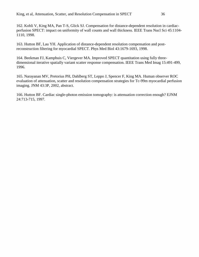
King, et al, Attenuation, Scatter, and Resolution Compensation in SPECT 36
162. Kohli V, King MA, Pan T-S, Glick SJ. Compensation for distance-dependent resolution in cardiac-perfusion SPECT: impact on uniformity of wall counts and wall thickness. IEEE Trans Nucl Sci 45:1104-1110, 1998.
163. Hutton BF, Lau YH. Application of distance-dependent resolution compensation and post-reconstruction filtering for myocardial SPECT. Phys Med Biol 43:1679-1693, 1998.
164. Beekman FJ, Kamphuis C, Viergever MA. Improved SPECT quantitation using fully three-dimensional iterative spatially variant scatter response compensation. IEEE Trans Med Imag 15:491-499,1996.
165. Narayanan MV, Pretorius PH, Dahlberg ST, Leppo J, Spencer F, King MA. Human observer ROCevaluation of attenuation, scatter and resolution compensation strategies for Tc-99m myocardial perfusionimaging. JNM 43:3P, 2002, abstract.
166. Hutton BF. Cardiac single-photon emission tomography: is attenuation correction enough? EJNM24:713-715, 1997.
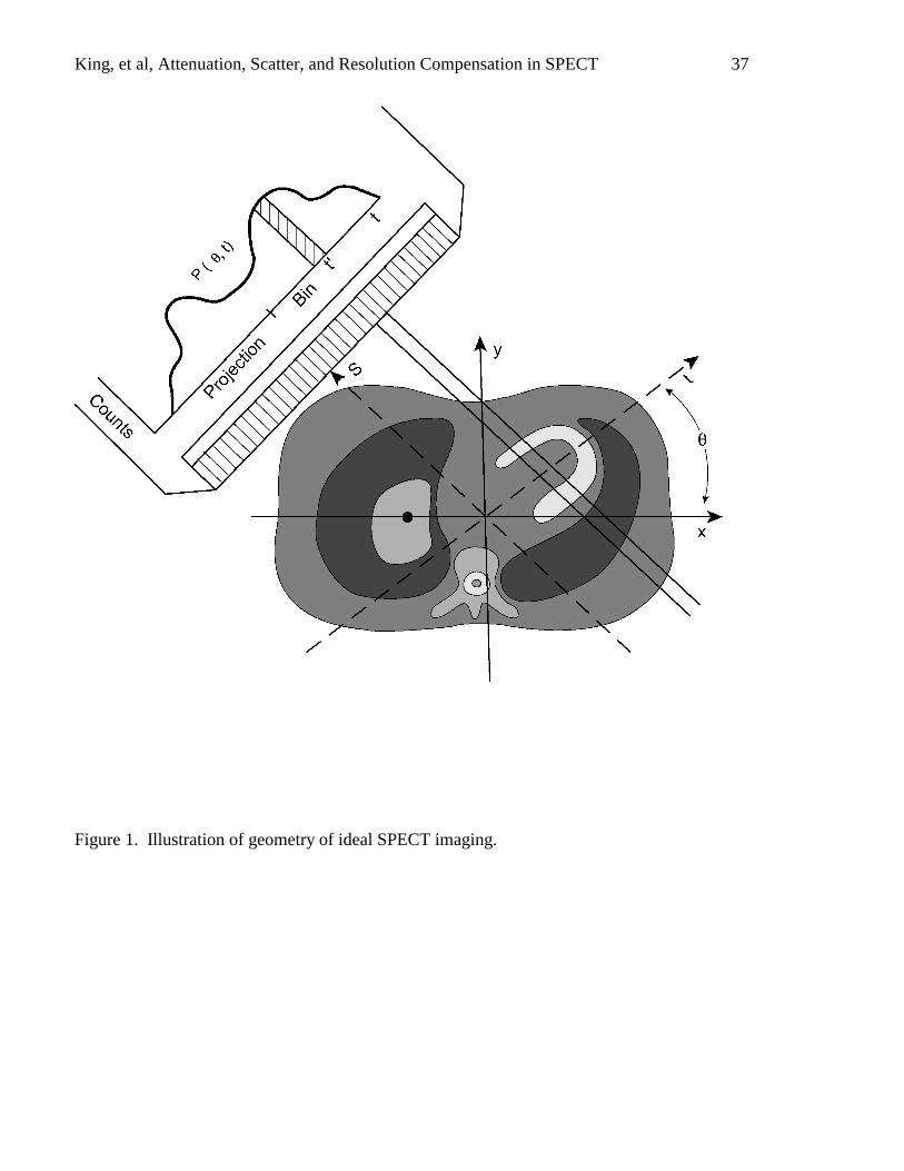
King, et al, Attenuation, Scatter, and Resolution Compensation in SPECT 37
Figure 1. Illustration of geometry of ideal SPECT imaging.
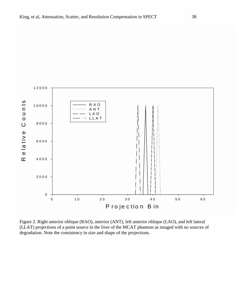
King, et al, Attenuation, Scatter, and Resolution Compensation in SPECT 38
P r o je c t io n B in
0 1 0 2 0 3 0 4 0 5 0 6 0
Re
lati
ve
Co
un
ts
0
2 0 0 0
4 0 0 0
6 0 0 0
8 0 0 0
1 0 0 0 0
1 2 0 0 0
R A OA N T L A OL L A T
Figure 2. Right anterior oblique (RAO), anterior (ANT), left anterior oblique (LAO), and left lateral(LLAT) projections of a point source in the liver of the MCAT phantom as imaged with no sources ofdegradation. Note the consistency in size and shape of the projections.
King, et al, Attenuation, Scatter, and Resolution Compensation in SPECT 39
Figure 3. Illustration of impact of attenuation on SPECT imaging. Note that photon A is stoppedphotoelectrically, and photon B is scattered such that it is not detected. The result is a decrease in thecounts in the projection data as illustrated.
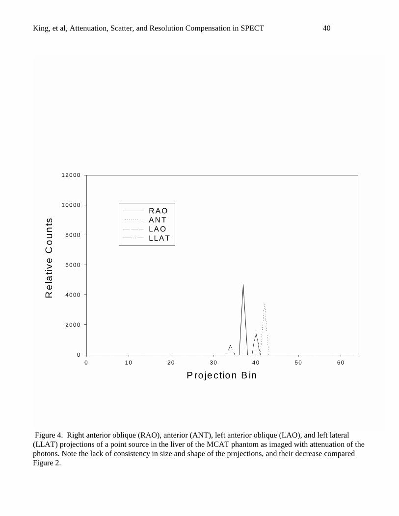
King, et al, Attenuation, Scatter, and Resolution Compensation in SPECT 40
P ro jection B in
0 10 20 30 40 50 60
Re
lati
ve
Co
un
ts
0
2000
4000
6000
8000
10000
12000
R AOAN TLAOLLAT
Figure 4. Right anterior oblique (RAO), anterior (ANT), left anterior oblique (LAO), and left lateral(LLAT) projections of a point source in the liver of the MCAT phantom as imaged with attenuation of thephotons. Note the lack of consistency in size and shape of the projections, and their decrease comparedFigure 2.

King, et al, Attenuation, Scatter, and Resolution Compensation in SPECT 41
Figure 5. Illustration of impact of scatter on SPECT imaging. Notice the addition of the photon from theliver scattered such that it appears at the incorrect location within the projections.
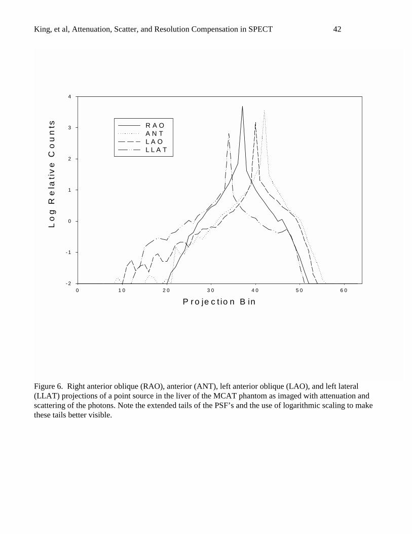
King, et al, Attenuation, Scatter, and Resolution Compensation in SPECT 42
P r o je c t io n B in
0 1 0 2 0 3 0 4 0 5 0 6 0
Lo
g R
ela
tiv
e C
ou
nts
- 2
- 1
0
1
2
3
4
R A OA N TL A OL L A T
Figure 6. Right anterior oblique (RAO), anterior (ANT), left anterior oblique (LAO), and left lateral(LLAT) projections of a point source in the liver of the MCAT phantom as imaged with attenuation andscattering of the photons. Note the extended tails of the PSF’s and the use of logarithmic scaling to makethese tails better visible.
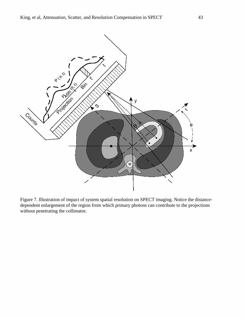
King, et al, Attenuation, Scatter, and Resolution Compensation in SPECT 43
Figure 7. Illustration of impact of system spatial resolution on SPECT imaging. Notice the distance-dependent enlargement of the region from which primary photons can contribute to the projectionswithout penetrating the collimator.
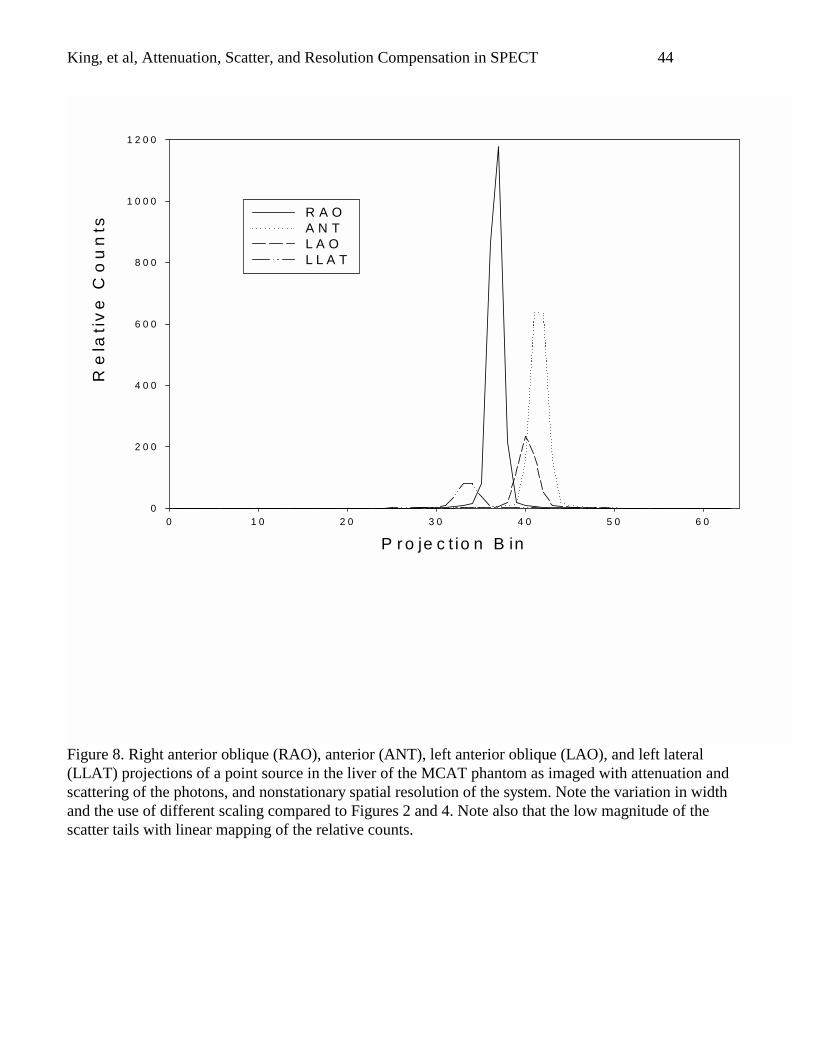
King, et al, Attenuation, Scatter, and Resolution Compensation in SPECT 44
P r o je c t io n B in
0 1 0 2 0 3 0 4 0 5 0 6 0
Re
lati
ve
Co
un
ts
0
2 0 0
4 0 0
6 0 0
8 0 0
1 0 0 0
1 2 0 0
R A OA N TL A OL L A T
Figure 8. Right anterior oblique (RAO), anterior (ANT), left anterior oblique (LAO), and left lateral(LLAT) projections of a point source in the liver of the MCAT phantom as imaged with attenuation andscattering of the photons, and nonstationary spatial resolution of the system. Note the variation in widthand the use of different scaling compared to Figures 2 and 4. Note also that the low magnitude of thescatter tails with linear mapping of the relative counts.
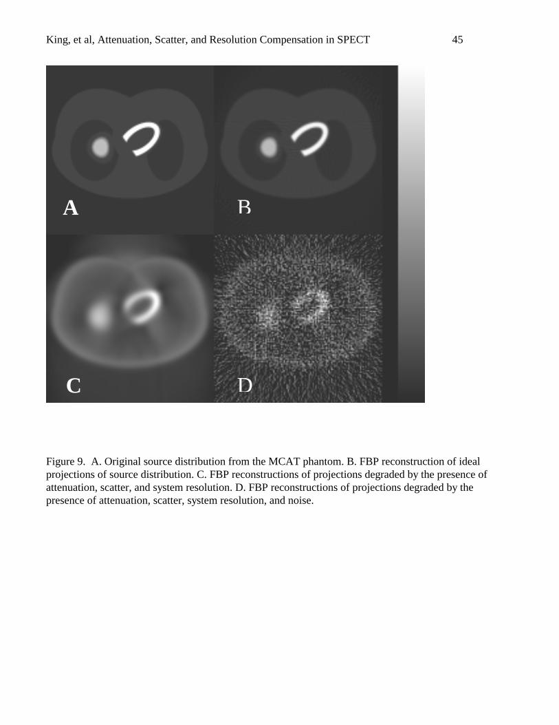
King, et al, Attenuation, Scatter, and Resolution Compensation in SPECT 45
Figure 9. A. Original source distribution from the MCAT phantom. B. FBP reconstruction of idealprojections of source distribution. C. FBP reconstructions of projections degraded by the presence ofattenuation, scatter, and system resolution. D. FBP reconstructions of projections degraded by thepresence of attenuation, scatter, system resolution, and noise.
C
A B
D
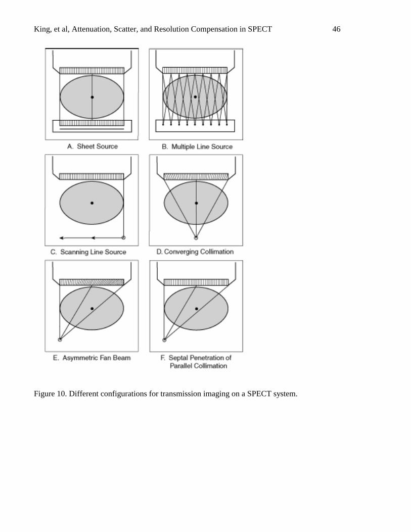
King, et al, Attenuation, Scatter, and Resolution Compensation in SPECT 46
Figure 10. Different configurations for transmission imaging on a SPECT system.
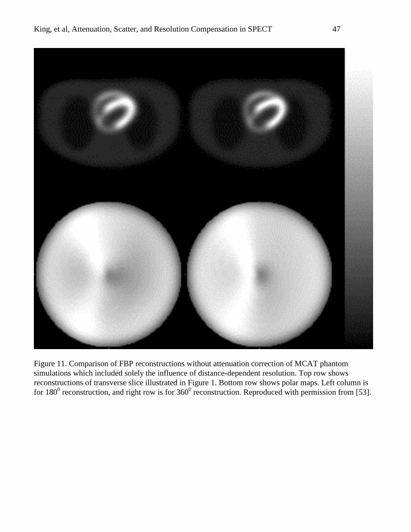
King, et al, Attenuation, Scatter, and Resolution Compensation in SPECT 47
Figure 11. Comparison of FBP reconstructions without attenuation correction of MCAT phantomsimulations which included solely the influence of distance-dependent resolution. Top row showsreconstructions of transverse slice illustrated in Figure 1. Bottom row shows polar maps. Left column isfor 1800 reconstruction, and right row is for 3600 reconstruction. Reproduced with permission from [53].
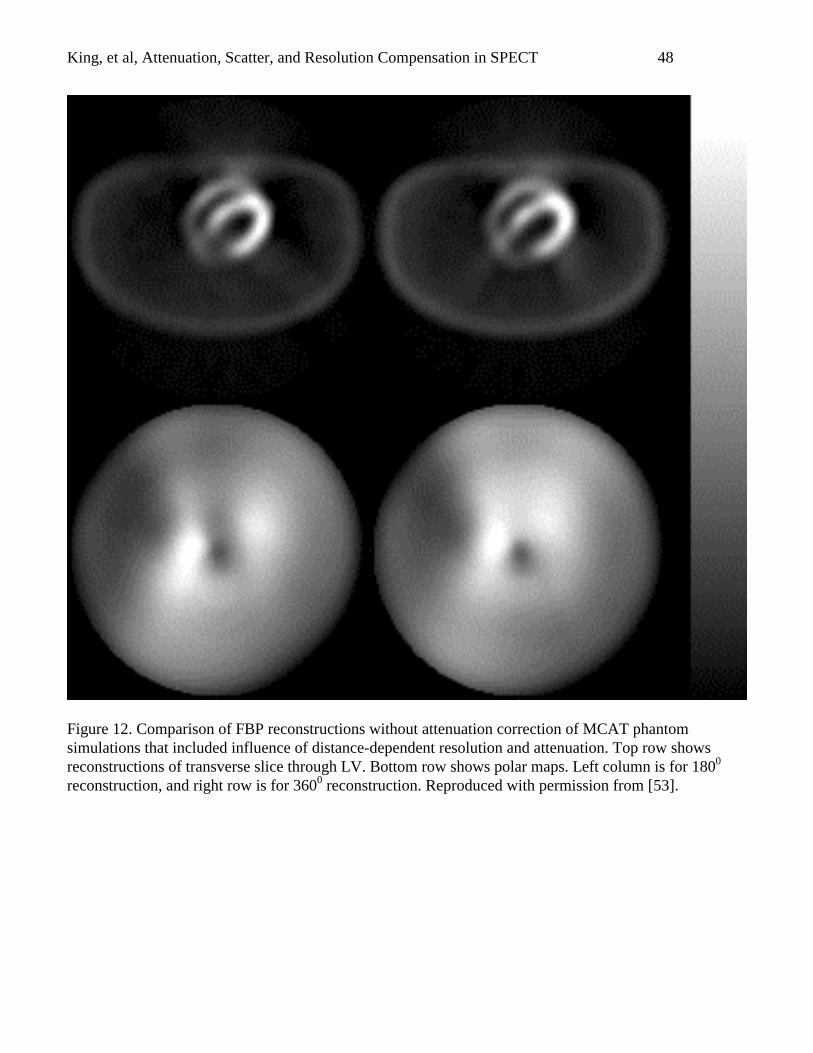
King, et al, Attenuation, Scatter, and Resolution Compensation in SPECT 48
Figure 12. Comparison of FBP reconstructions without attenuation correction of MCAT phantomsimulations that included influence of distance-dependent resolution and attenuation. Top row showsreconstructions of transverse slice through LV. Bottom row shows polar maps. Left column is for 1800
reconstruction, and right row is for 3600 reconstruction. Reproduced with permission from [53].
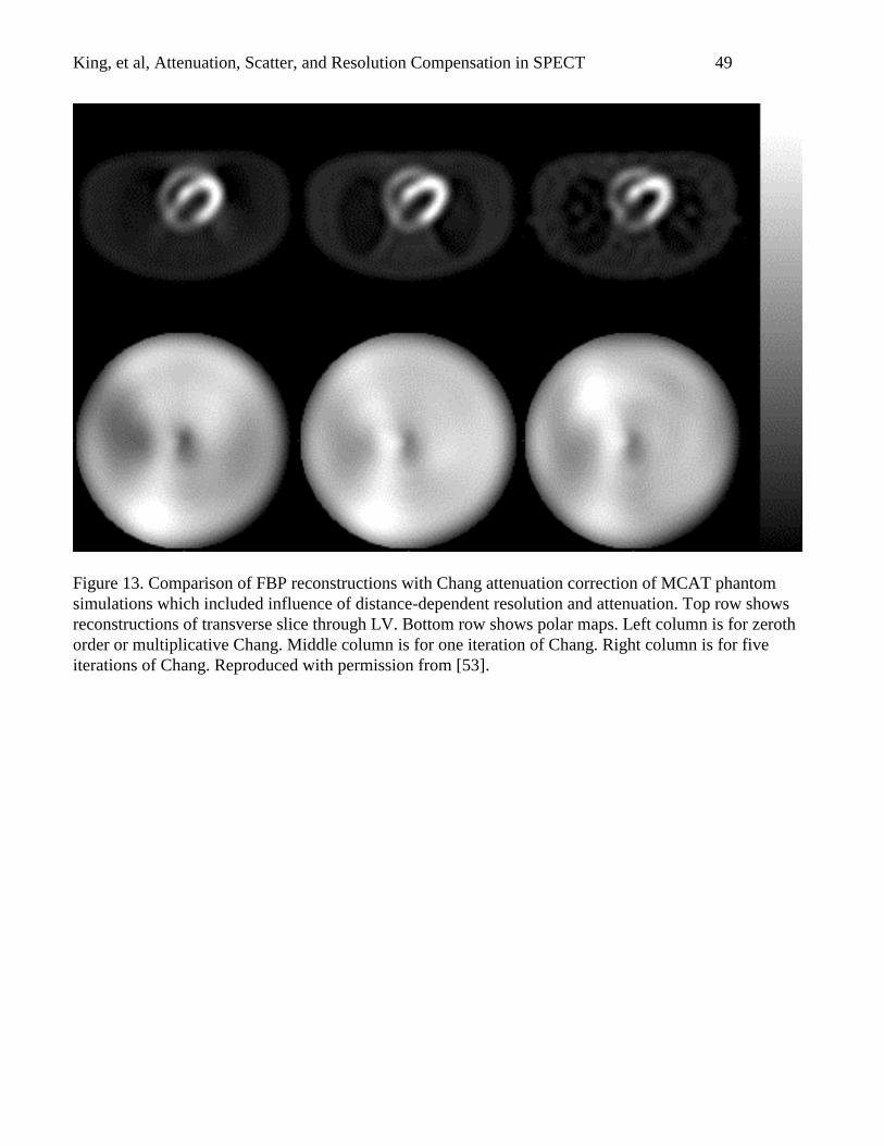
King, et al, Attenuation, Scatter, and Resolution Compensation in SPECT 49
Figure 13. Comparison of FBP reconstructions with Chang attenuation correction of MCAT phantomsimulations which included influence of distance-dependent resolution and attenuation. Top row showsreconstructions of transverse slice through LV. Bottom row shows polar maps. Left column is for zerothorder or multiplicative Chang. Middle column is for one iteration of Chang. Right column is for fiveiterations of Chang. Reproduced with permission from [53].
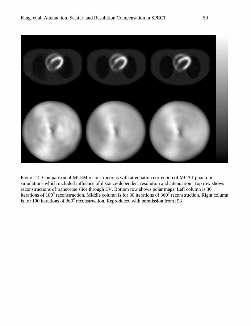
King, et al, Attenuation, Scatter, and Resolution Compensation in SPECT 50
Figure 14. Comparison of MLEM reconstructions with attenuation correction of MCAT phantomsimulations which included influence of distance-dependent resolution and attenuation. Top row showsreconstructions of transverse slice through LV. Bottom row shows polar maps. Left column is 30iterations of 1800 reconstruction. Middle column is for 30 iterations of 3600 reconstruction. Right columnis for 100 iterations of 3600 reconstruction. Reproduced with permission from [53].
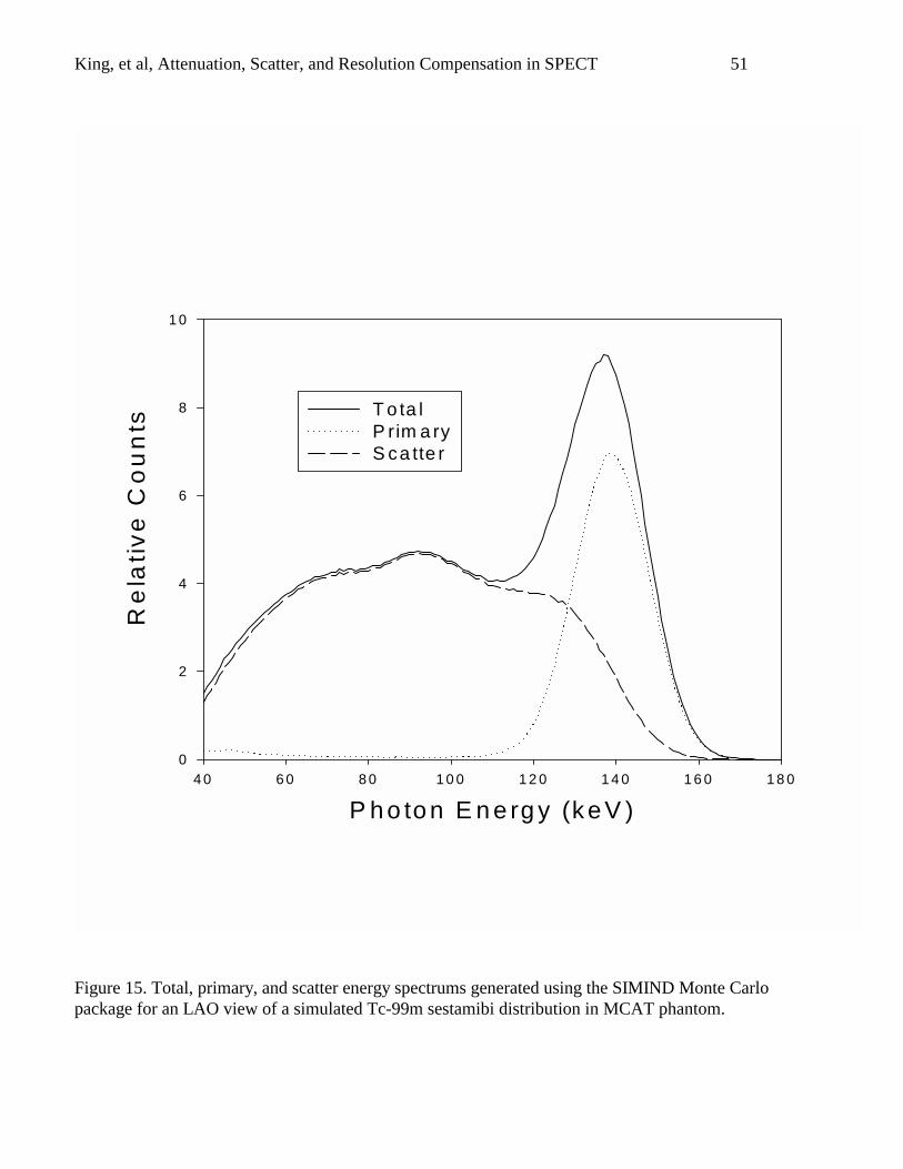
King, et al, Attenuation, Scatter, and Resolution Compensation in SPECT 51
P h o to n E n e rg y (ke V )
4 0 6 0 8 0 1 0 0 1 2 0 1 4 0 1 6 0 1 8 0
Re
lati
ve
Co
un
ts
0
2
4
6
8
1 0
T o ta lP rim a ryS ca tte r
Figure 15. Total, primary, and scatter energy spectrums generated using the SIMIND Monte Carlopackage for an LAO view of a simulated Tc-99m sestamibi distribution in MCAT phantom.
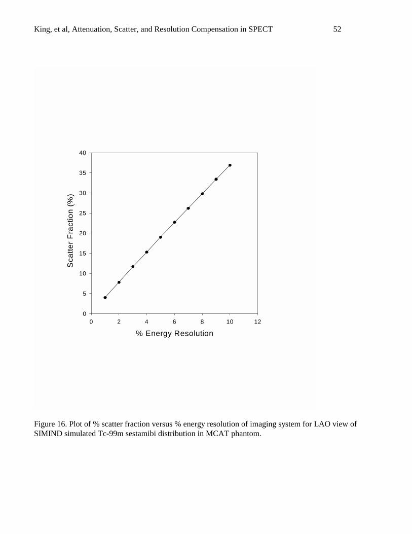
King, et al, Attenuation, Scatter, and Resolution Compensation in SPECT 52
% Energy Resolution
0 2 4 6 8 10 12
Sca
tte
r F
ract
ion
(%
)
0
5
10
15
20
25
30
35
40
Figure 16. Plot of % scatter fraction versus % energy resolution of imaging system for LAO view ofSIMIND simulated Tc-99m sestamibi distribution in MCAT phantom.
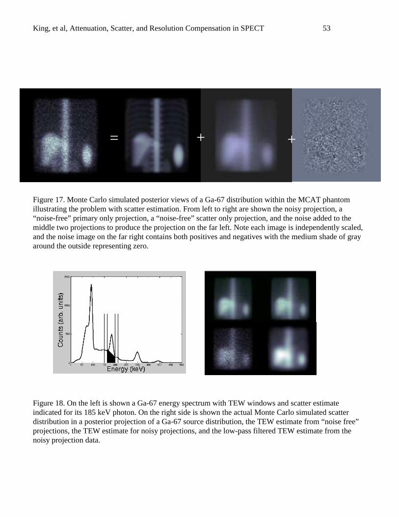
King, et al, Attenuation, Scatter, and Resolution Compensation in SPECT 53
Figure 17. Monte Carlo simulated posterior views of a Ga-67 distribution within the MCAT phantomillustrating the problem with scatter estimation. From left to right are shown the noisy projection, a“noise-free” primary only projection, a “noise-free” scatter only projection, and the noise added to themiddle two projections to produce the projection on the far left. Note each image is independently scaled,and the noise image on the far right contains both positives and negatives with the medium shade of grayaround the outside representing zero.
Figure 18. On the left is shown a Ga-67 energy spectrum with TEW windows and scatter estimateindicated for its 185 keV photon. On the right side is shown the actual Monte Carlo simulated scatterdistribution in a posterior projection of a Ga-67 source distribution, the TEW estimate from “noise free”projections, the TEW estimate for noisy projections, and the low-pass filtered TEW estimate from thenoisy projection data.
= + +
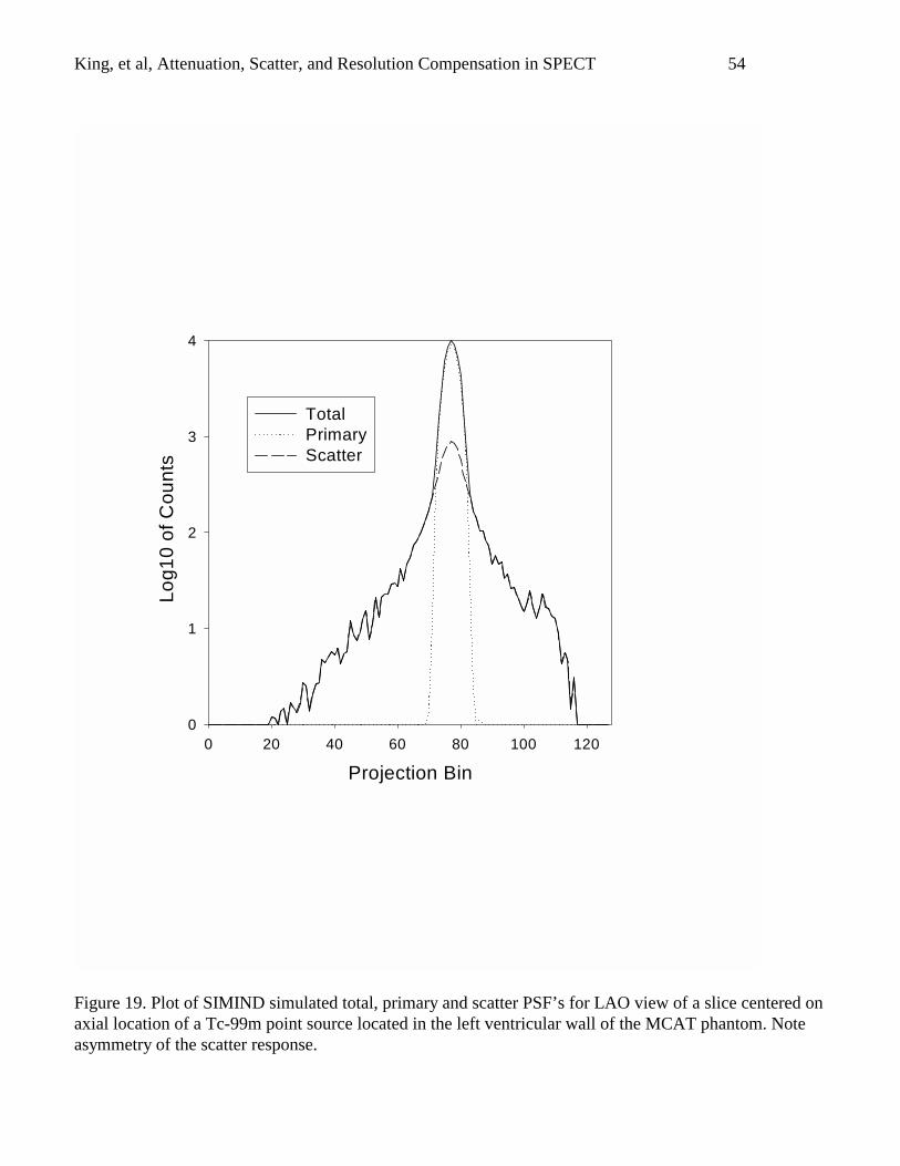
King, et al, Attenuation, Scatter, and Resolution Compensation in SPECT 54
Projection Bin
0 20 40 60 80 100 120
Lo
g1
0 o
f C
ou
nts
0
1
2
3
4
TotalPrimaryScatter
Figure 19. Plot of SIMIND simulated total, primary and scatter PSF’s for LAO view of a slice centered onaxial location of a Tc-99m point source located in the left ventricular wall of the MCAT phantom. Noteasymmetry of the scatter response.
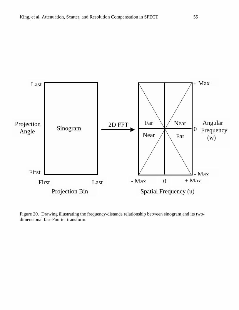
King, et al, Attenuation, Scatter, and Resolution Compensation in SPECT 55
Figure 20. Drawing illustrating the frequency-distance relationship between sinogram and its two-dimensional fast-Fourier transform.
Projection Angle
Last
First
2D FFT
+ Max
Angular Frequency (w)
0
+ Max
- Max
Far
Far
Near
Near
- Max 0
Spatial Frequency (u)
Sinogram
First Last
Projection Bin
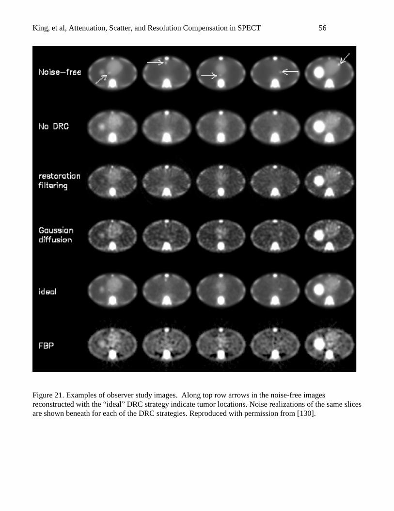
King, et al, Attenuation, Scatter, and Resolution Compensation in SPECT 56
Figure 21. Examples of observer study images. Along top row arrows in the noise-free imagesreconstructed with the “ideal” DRC strategy indicate tumor locations. Noise realizations of the same slicesare shown beneath for each of the DRC strategies. Reproduced with permission from [130].