This article was downloaded by: [Jérôme Pousin]On: 04 December 2012, At: 01:49Publisher: Taylor & FrancisInforma Ltd Registered in England and Wales Registered Number: 1072954 Registeredoffice: Mortimer House, 37-41 Mortimer Street, London W1T 3JH, UK

Applicable Analysis: An InternationalJournalPublication details, including instructions for authors andsubscription information:http://www.tandfonline.com/loi/gapa20

A posteriori estimate and asymptoticpartial domain decompositionGustavo C. Buscaglia a , Jérôme Pousin b & Kamel Slimani ba Instituto de Ciências Matemáticas e de Computação, Av. doTrabalhador Sãocarlense 400, Centro, CEP 13560-970 São Carlos,SP, Brasilb Université de Lyon CNRS, INSA-Lyon ICJ UMR 5208, bat. L. deVinci, 20 Av. A. Einstein, F-69100 Villeurbanne Cedex, FranceVersion of record first published: 04 Dec 2012.

To cite this article: Gustavo C. Buscaglia , Jérôme Pousin & Kamel Slimani (2012): A posterioriestimate and asymptotic partial domain decomposition, Applicable Analysis: An InternationalJournal, DOI:10.1080/00036811.2012.746965

To link to this article: http://dx.doi.org/10.1080/00036811.2012.746965

PLEASE SCROLL DOWN FOR ARTICLE

Full terms and conditions of use: http://www.tandfonline.com/page/terms-and-conditions

This article may be used for research, teaching, and private study purposes. Anysubstantial or systematic reproduction, redistribution, reselling, loan, sub-licensing,systematic supply, or distribution in any form to anyone is expressly forbidden.

The publisher does not give any warranty express or implied or make any representationthat the contents will be complete or accurate or up to date. The accuracy of anyinstructions, formulae, and drug doses should be independently verified with primarysources. The publisher shall not be liable for any loss, actions, claims, proceedings,demand, or costs or damages whatsoever or howsoever caused arising directly orindirectly in connection with or arising out of the use of this material.

Applicable Analysis2012, 1–17, iFirst

A posteriori estimate and asymptotic partial domain decomposition

Gustavo C. Buscagliaa, Jerome Pousinb* and Kamel Slimanib

aInstituto de Ciencias Matematicas e de Computacao, Av. do Trabalhador Saocarlense400, Centro, CEP 13560-970 Sao Carlos, SP, Brasil; bUniversite de Lyon CNRS,

INSA-Lyon ICJ UMR 5208, bat. L. de Vinci, 20 Av. A. Einstein,F-69100 Villeurbanne Cedex, France

Communicated by G. Panasenko

(Received 1 May 2012; final version received 1 November 2012)

The method of asymptotic partial decomposition of a domain aims atreplacing a 3D or 2D problem by a hybrid problem 3D� 1D; or 2D� 1D,where the dimension of the problem decreases in part of the domain.The location of the junction between the heterogeneous problems isasymptotically estimated in certain circumstances, but for numericalsimulations it is important to be able to determine the location of thejunction accurately. In this article, by reformulating the problem in a mixedformulation context and by using an a posteriori error estimate, we proposean indicator of the error due to a wrong position of the junction.Minimizing this indicator allows us to determine accurately the location ofthe junction. Some numerical results are presented for a toy problem.

Keywords: asymptotic partial domain decomposition; a posteriori errorestimates; error indicator

AMS Subject Classifications: 35F40; 65

1. Introduction

The method of asymptotic partial decomposition of a domain (MAPDD) originatesfrom the works of Panasenko [1]. The idea is to replace an original 3D or 2Dproblem by a hybrid one 3D� 1D; or 2D� 1D, where the dimension of the problemdecreases in part of the domain. Effective solution methods for the resulting hybridproblem have recently become available for several systems (linear/nonlinear, fluid/solid, etc.) which allow for each subproblem to be computed with an independentblack-box code [2–4]. The location of the junction between the heterogeneousproblems is asymptotically estimated in the works of Panasenko [5]. MAPDD hasbeen designed for handling problems where a small parameter appears, and providesa series expansion of the solution with solutions of simplified problems with respect

*Corresponding author. Email: jerome.pousin@insa-lyon.fr

ISSN 0003–6811 print/ISSN 1563–504X online

� 2012 Taylor & Francis

http://dx.doi.org/10.1080/00036811.2012.746965

http://www.tandfonline.com

Dow

nloa

ded

by [

Jérô

me

Pous

in]

at 0

1:49

04

Dec

embe

r 20

12

to this small parameter. In the problem considered here, no small parameter exists,but due to geometrical considerations concerning the domain � it is assumed that thesolution does not differ very much from a function which depends only on onevariable in a part of the domain. The MAPDD theory is not suited for such acontext, but if this theory is applied formally it does not provide any error estimate.The a posteriori error estimate proved in this article, is able to measure thediscrepancy between the exact solution and the hybrid solution which corresponds tothe zero-order term in the series expansion with respect to a small parameter whenit exists.

Numerically, independently of the existence of an asymptotical estimate of thelocation of the junction, it is essential to detect with accuracy the location of thejunction. Let us also mention the interest of locating with accuracy the position ofthe junction in blood flows simulations [6]. Here the method proposed is todetermine the location of the junction (i.e. the location of the boundary � in theexample treated) by using optimization techniques. First it is shown thatMAPDD can be expressed with a mixed domain decomposition formulation(as in [5,7–12]) in two different ways. Then it is proposed to use an a posteriori errorestimate for locating the best position of the junction. A posteriori error estimateshave been extensively used in optimization problems, the reader is referred to,e.g. [8,9].

In the following, the toy problem for which the method is presented is given, andthe introduction section is ended with the mixed formulation of the domaindecomposition of the problem. Section 2 is dedicated to the two asymptoticdecompositions proposed for a given location of the interface �. Oneasymptotic decomposition is based on a particular mortar subspace (the constantfunctions on �), and the other one is based on coupling a partial differential equation(PDE) with an ordinary differential equation (ODE). In Section 3, a posteriori errorestimates are given and an indicator is proposed. In Section 4, the optimal location ofthe junction is found by minimizing the indicator. Numerical results are providedshowing the efficiency of the proposed method.

Let f be a regular function defined by

f ðx1, x2Þ ¼f1ðx1, x2Þ, 05 x1 5 a,

f2ðx1Þ, a5 x5 1:

�ð1Þ

The domain �¼ (0, 1)� (0, 1) is decomposed in two subdomains �1¼ (0, a)� (0, 1)and �2¼ (a, 1)� (0, 1), the boundary � ¼ �1 \�2, and the boundary @� are dividedinto four subparts �1¼ {0}� (0, 1) �2¼ (0, 1)� {0} �3¼ {1}� (0, 1) �4¼ (0, 1)� {1}.

2 G.C. Buscaglia et al.

Dow

nloa

ded

by [

Jérô

me

Pous

in]

at 0

1:49

04

Dec

embe

r 20

12

Let U2H2(�) be the solution to:

�DUðx1, x2Þ ¼ f ðx1,x2Þ, in �,

@nU ¼ 0, on �2i; 1 � i � 2;

U ¼ 0, on �2i�1; 1 � i � 2:

8><>: ð2Þ

Now let us give a formulation of the problem in the domain decomposition context

with a L2-mortar subspace. We define the following functional spaces:

0H1ð�1Þ ¼ f’2H

1ð�1Þ, ’j�1 ¼ 0g,

0H1ð�2Þ ¼ f’2H

1ð�2Þ, ’j�3 ¼ 0g,

V ¼0 H1ð�1Þ �0 H

1ð�2Þ,

W ¼0 H1ð�1Þ �0 H

1ð�2Þ \ fD2’j�2¼ 0g,

� ¼ L2ð�Þ,

ð3Þ

equipped with the norms

jvj21 ¼X2i¼1

Z�i

rvi � rvi dx1 dx2, k�k2� ¼

Z�

�2 dx2: ð4Þ

Let us define (u1, u2, �)2V�� solution to

X2i¼1

Z�i

rui � rvi dx1 dx2 þ

Z�

�ðv1 � v2Þdx2 ¼X2i¼1

Z�i

fvi dx1 dx2, 8v2V

Z�

�ðu1 � u2Þ dx2 ¼ 0, 8�2�:

8>>><>>>:

ð5Þ

Introduce the following bilinear forms:

a :V� V�!R

u, v 7 �! aðu, vÞ ¼X2i¼1

Z�i

ruirvi dx1dx2,

b : �� V�!R

�, v 7 �! bð�, vÞ ¼

Z�

�ðv1 � v2Þdx2:

We have the following result.

LEMMA 1.1 Assume f2L2(�) then, there exists a unique (u1, u2, �)2V�� solution

to problem (5). Moreover, we have ui ¼ Uj�ifor 1� i� 2.

Proof Let K be the closed subset of space V defined by

K ¼ fv2V; v1 � v2j� 2�?g:

The existence result is a consequence of the following inf-sup condition: there exists

05� such that

infðw,�Þ 2K��

supðv,�Þ6¼ð0,0Þ 2V��

aðw, vÞ þ bð�, vÞ þ bð�,wÞ

k�k� þ jvj1� �: ð6Þ

Applicable Analysis 3

Dow

nloa

ded

by [

Jérô

me

Pous

in]

at 0

1:49

04

Dec

embe

r 20

12

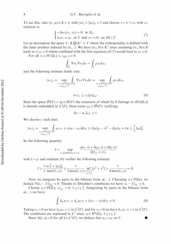
To see this, take (w, �)2K�� with jwj1þk�k�¼ 1 and choose v¼wþw1 with w1

solution to

�Dw1ðx1, x2Þ ¼ 0, in �1,

@nw1 ¼ �, on � and w1 ¼ 0, on @� n �:

�ð7Þ

Let us decompose the space V :KL

K? ¼ V where the orthogonality is defined with

the inner product induced by a(., .). We have (w1, 0)2K? since assuming (w1, 0)2K

leads to w1j�¼ 0 which combined with the first equation of (7) would lead to w1¼ 0.For all v1 2H

1ð�1Þ, v1 j@�1n�¼ 0Z�1

rw1rv1dx ¼

Z�

�v1dx2

and the following estimate holds true:

jw1j1 ¼ supv1 2H1ð�1Þv1 j@�1n�

¼0

Z�1

rw1rv1dx ¼ supv1 2H1ð�1Þv1 j@�1n�

¼0

Z�

�v1dx2,

jw1j1 � c2k�k0,�: ð8Þ

Since the space ~H12ð�Þ ¼ f’2H

12ð�Þ the extension of which by 0 belongs to H

12ð@�1Þg

is densely embedded in L2(�), there exists �" 2 ~H12ð�Þ: verifying:

k�� �"k0,� � ":

We choose " such that:

jw1j1 ¼ supv1 2H1ð�1Þv1 j@�1n�

¼0

Z�

�"v1 þ v1ð�� �"Þdx2 � ðk�k0 � "Þ2� ðk�k0 þ "Þ" �

1

2k�k20:

So the following quantity

I ¼ supðv,�Þ6¼ð0,0Þ 2V��

aðw, vÞ þ bð�, vÞ þ bð�,wÞ

k�k� þ jvj1

with �¼� and estimate (8) verifies the following estimate

I �1

2

jwj21 þ k�k20

maxð1, c2Þ�

1

2maxð1, c2Þinf

xþy¼1x�0, y�0

½x2 þ y2� �1

4maxð1, c2Þ¼ �:

Now we integrate by parts in the bilinear form a(�, �). Choosing vi2D(�i), we

deduce rðui �UÞj�i¼ 0. Thanks to Dirichlet’s conditions we have: ui �Uj�i

¼ 0.Choose vi 2Dð�iÞ; vij�2i ¼ 0; 1� i� 2. Integrating by parts in the bilinear form

a(�, �) we have: Z�

@n1u1v1 þ @n2u2v2 þ �ðv1 � v2Þ dx2 ¼ 0: ð9Þ

Taking v1¼ 0 we have @n2u2 ¼ � in L2(�) and for v2¼ 0 we have @n1u1 ¼ �� in L2(�).

The conditions are expressed in L2 since, ui2H2(�i), 1� i� 2.

Since b(�, u)¼ 0 for all �2L2(�), we deduce that u1¼ u2 on �. g

4 G.C. Buscaglia et al.

Dow

nloa

ded

by [

Jérô

me

Pous

in]

at 0

1:49

04

Dec

embe

r 20

12

2. Asymptotic domain decomposition

In this section, we propose two approximate domain decomposition problems by

using different mortar subspaces or different spaces for the solution. Let

�0¼ span{1} and let us define (u1, u2, �0)2V��0 solution of

að ~u, vÞ þ bð�0, vÞ ¼X2i¼1

Z�i

fvi dx1dx2, 8v2V,

bð�, ~uÞ ¼ 0, 8�2�0:

8><>: ð10Þ

LEMMA 2.1 Assume f2L2(�), then, there exists a unique (u1, u2, �0)2V��0

solution to problem (10). Moreover, we have

@n1 ~u1 ¼ �@n2 ~u2, in L2ð�Þ, ~u2j� ¼1

j�j

Z�

~u1 dx2:

Proof The existence result is a consequence of the inf-sup condition, which is

proved in the same way as in Lemma 1.1 with w1¼ cx1, and

�?0 ¼ f’2L2ð�Þ;

Z�

’ðx2Þdx2 ¼ 0g ) ðw1, 0Þ 2K?:

Integrating by parts in (10), thus, since ui2H2(�i), we have

@n2 ~u2j� ¼ �0 2�0:

Take v2¼ 0, whatever v1 is:

R�ð@n1 ~u1 þ �0Þv1dx2 ¼ 0) @n1 ~u1 þ �0 ¼ 0 in ~H

12ð�Þ0 ) @n1 ~u1 ¼ ��0:

Now, let us prove that u2W. Since �0 is constant, it is easy to prove that u2(x1)

solution to

� ~u002ðx1Þ ¼ f2ðx1Þ, in a5 x1 5 1,

~u02ðx1Þ ¼ �0, ~u2ð1Þ ¼ 0,

�

is the unique solution u2 in the domain �2.The condition b(1, u)¼ 0 implies ~u2 ¼

1�

R�

~u1 dx2: g

Remark 1 The previous result provides a justification for coupling an ODE with a

PDE in some circumstances which can also be justified with asymptotic

developments.

Now, set �2¼L2(�) as mortar subspace, and let us define (u1, u2, �2)2W��2

solution to

aðu, vÞ þ bð�2, vÞ ¼X2i¼1

Z�i

fvi dx1dx2, 8v2V,

bð�, uÞ ¼ 0, 8�2�2:

8><>: ð11Þ

Applicable Analysis 5

Dow

nloa

ded

by [

Jérô

me

Pous

in]

at 0

1:49

04

Dec

embe

r 20

12

LEMMA 2.2 Assume f2L2(�), then, there exists a unique (u1, u2, �2)2W��2

solution to problem (11). Moreover, we have

@n2 u2 ¼ �1

j�j

Z�

@n1 u1 dx2 u1 ¼ u2, in L2ð�Þ:

Proof The space W is a closed subspace of V thus the existence is proved in the

same way as in the previous lemma. The identity (9) with v1¼ 0 reads: for everyv22L

2(�)

Z�

ð@n2 u2 � �2Þv2dx2 ¼ 0: ð12Þ

Since @n2 u2 � �2 2�?2 we conclude that @n2 u2 ¼ �2. Take v2¼ 0, for every v12L2(�),

identity (9) reads: Z�

ð@n1 u1 þ �2Þv1dx2 ¼ 0) @n1 u1 ¼ ��2, in �2: ð13Þ

Since u22W, the relation (12) reads: @n2 u2 ¼ �1j�j

R� @n1 u1 dx2. The condition

b(�, u)¼ 0 for every �2�2 implies u2¼ u1. g

3. A posteriori error estimates

In this section an a posteriori error estimate is derived for the error between the exactsolution of the domain decomposition formulation of the problem, and the

approximate solution by using a mortar subspace.Let us define the operatorT : V�L

2(�)!V0 �L2(�)0 by

hTð ~u, �0Þ, ðv, �Þi ¼ að ~u, vÞ þ bð�0, vÞ þ bð�, ~uÞ:

Define the error e by

e ¼ ðu� ~u, �� �0Þ: ð14Þ

In what follows, an indicator for the error is proposed.The error equation reads:

hTe, ðv, �Þi ¼ aððu� ~uÞ, vÞ þ bð�� �0, vÞ þ bð�, u� ~uÞ

¼ �

Z�

ð@n1 ~u1v1 þ @n2 ~u2v2dx2 �

Z�

�0ðv1 � v2Þdx2 �

Z�

�ð ~u1 � ~u2Þ dx2

¼ L ~u, �0ðv, �Þ: ð15Þ

LEMMA 3.1 Assume f2L2(�), then, the following estimate holds true.

kL ~u, �0k�

kTkL� kek � kL ~u, �0k�kT

�1kL, ð16Þ

6 G.C. Buscaglia et al.

Dow

nloa

ded

by [

Jérô

me

Pous

in]

at 0

1:49

04

Dec

embe

r 20

12

with

kL ~u, �0k� ¼ k ~u1 �1

j�j

Z�

~u1 dx2k0,�,

� � kTkL; kT�1kL �1

�:

ð17Þ

Proof We have to evaluate:

kL ~u, �0k� ¼ supðv, �Þ 2V��ðv,�Þ6¼ð0,0Þ

aðu� ~u, vÞ þ bð�� �0, vÞ þ bð�, u� ~uÞ

k�k0,� þ jvj1:

ð18Þ

Observe that by integrating by parts in the bilinear form a(�, �), we have

aðu� ~u, vÞ ¼ �

Z�

@n1 ~u1v1 þ @n2 ~u2v2dx2 �

Z�

�ðv1 � v2Þdx2:

Gathering (18) with the previous inf-sup condition, we deduce

kek �1

�sup

ðv, �Þ 2V��ðv,�Þ6¼ð0,0Þ

�R

�@n1 ~u1v1 þ @n2 ~u2v2dx2 þ bð��0, vÞ þ bð�, u� ~uÞ

k�k0,� þ jvj1, ð19Þ

which proves the bound from above in (16). Accounting for the relation between

@n1 ~u1,@n1 ~u2 and �0 given in Lemma 2.1 we have:

kek �1

�sup

ðv, �Þ 2V��ðv,�Þ6¼ð0,0Þ

�R

� �ð ~u1 � ~u2Þ dx2

k�k0,� þ jvj1,

and finally

kek �1

�k ~u1 � ~u2k0,� ¼

1

�k ~u1 �

1

j�j

Z�

~u1 dx2k0,�: ð20Þ

Now, let us consider the second case where f2L2(�) and the mortar subspace is

�2¼L2(�). Starting from the inequality (19) accounting for results of Lemma 2.2

arguing in the same way as before, we get the following indicator:

kek �1

�k@n1 u1 þ @n2 u2k0,� ¼

1

�k@n1 u1 �

1

j�j

Z�

@n1 u1dx2k0,�: ð21Þ

4. Optimization with respect to the location of �

Let a denote the position of the boundary �. Due to relation (20), the proposed

strategy is to minimize the functional J(a) with respect to a defined by

JðaÞ ¼ k ~u1ða, x2Þ �1

j�aj

Z�a

~u1ða, x2Þ dx2k20,�:

Applicable Analysis 7

Dow

nloa

ded

by [

Jérô

me

Pous

in]

at 0

1:49

04

Dec

embe

r 20

12

The algorithm of minimization we propose is a simple descent algorithm. Let a0 and

Tol be fixed.

(1) evaluate the derivative DJ(an)(2) if jDJ(an)j �Tol stop and if not(3) anþ1¼ an� � DJ(an) where � is a fixed positive number.(4) n¼ nþ 1 return to the beginning.

Now we evaluate numerically the derivative with respect to the location of the

boundary �. To compute DJ(an) define:

Iða,x2Þ ¼ ~u1ða, x2Þ �

Z 1

0

~u1ða, x2Þdx2:

Observe that

JðaÞ ¼ ðIða,x2Þ, Iða, x2ÞÞL2ð�Þ,

its derivative DJðaÞ ¼ 2�@Iða,x2Þ@a

�, Iða,x2ÞL2ð�Þ where:

@I

@aða,x2Þ ¼

@ ~u1@aða, x2Þ �

Z 1

0

@ ~u1@aða, x2Þdx2:

To compute the derivative of u1 with respect to 05 a5 1, the location of �a we use

the following change of geometry which consists in mapping the domain � with a

moving boundary �a onto a domain with a fixed boundary �1/2. Thus the change of

geometry will yield a change in coefficients of PDEs. Define the transformation T by

½0, 1� � ½0, 1� ! ½0, 1� � ½0, 1�,

ðz, x2Þ ! ðx1, x2Þ ¼ ðTðz, aÞ ¼ ð2� 4aÞz2 þ ð4a� 1Þz, x2Þ,

thus the segment �12is mapped to �a. The unknown is defined by ¼U T.

Equation (2) becomes:

�DzT:D2zz � ðDzTÞ

3:D2x2x2

þD2zzT:Dz ¼ ðDzTÞ

3:f ðT, x2Þ,

@n ¼ 0 on �2i; 1 � i � 2,

¼ 0 on �2i�1; 1 � i � 2:

8><>: ð22Þ

A variational formulation for the decomposed domain problem corresponding

to the problem (22) with a mortar subspace �0 is: �1 ¼ ð0,12Þ � ð0, 1Þ and

�2 ¼ ð12 , 1Þ � ð0, 1Þ;

X2i¼1

Z�i

cðzÞ:r ~ i:rvi dx1dx2 þ 2X2i¼1

Z�i

D2zzT:Dz

~ i:vi dx1dx2

þ

Z�a

�ðv1 � v2Þ dx2 ¼X2i¼1

Z�i

ðDzTÞ3:fiðT, x2Þ:vi dx1dx2, 8v2V

Z�

�ð ~ 1 � ~ 2Þ dx2 ¼ 0, 8�2�0,

8>>>>>>>>><>>>>>>>>>:

ð23Þ

8 G.C. Buscaglia et al.

Dow

nloa

ded

by [

Jérô

me

Pous

in]

at 0

1:49

04

Dec

embe

r 20

12

where c is 2� 2 diagonal matrix such as c11¼DzT and c22¼ (DzT)3. Now we

calculate the derivative of the indicator J(a) with respect to a with function ~ :

DJðaÞ ¼ 2

Z 1

0

~u1ða, x2Þ �

Z 1

0

~u1ða, x2Þ dx2

� �@I

@aða, x2Þ dx2,

therefore,

DJðaÞ ¼ 2

Z 1

0

�~�1 �

Z 1

0

~�1dx2

��

�~�1a �

Z 1

0

~�1adx2

�dx2,

where ~�ia denotes the derivative with respect to a of function ~�i for 1� i� 2. In the

case where f2L2(�) and �2¼L2(�) we use the indicator given in (21), we have:

JðaÞ ¼

Z 1

0

ð@n1 u1ða, x2Þ �

Z 1

0

@n1 u1ða, x2Þdx2Þ2dx2, ð24Þ

DJðaÞ ¼ 2

Z 1

0

�@x1�1 �

Z 1

0

@x1�1dx2Þ

��@x1�1a �

Z 1

0

@x1�1adx2Þ

�dx2, ð25Þ

where �ia is the derivative of �i with respect to the variable a. Taking the derivative

of the first equation of (22) with respect to the variable a we have:

�DzT �D3azz��ðDzTÞ

3�D3

ax2x2�þD2

zzT �D2az�¼D2

azT �D2zz�þ3D2

az � ðDzTÞ2�D2

x2x2�

�D3azzT �Dz�þ3D2

azT � ðDzTÞ2� fðT,x2ÞþDaTðDzTÞ

3�Dx1 fðT,x2Þ: ð26Þ

Defining �a¼Da� Equation (26) becomes:

�DzT �Dzz�a�ðDzTÞ3�D2

x2x2�aþD2

zzT �Dz�a¼D2azT �D

2zz�þ3D2

azT � ðDzTÞ2�D2

x2x2�

�D3azzT �Dz�þ3D2

azT � ðDzTÞ2� f ðT,x2ÞþDaTðDzTÞ

3�Dx1 fðT,x2Þ,

@n�a¼ 0, on �2i; 1� i� 2,

�a¼ 0, on �2i�1; 1� i� 2:

8>>>><>>>>:

ð27Þ

A variational formulation for problem (27) in decomposed domain setting is:

X2i¼1

Z�i

ðcðzÞr ~ iarvi þ 2D2zzTDz

~ iaviÞdx1dx2 þ

Z�a

�ðv1 � v2Þdx2

¼X2i¼1

Z�i

ð�caðzÞr ~ irvi � 2D3azzTDz

~ iviÞdx1dx2

þX2i¼1

Z�i

½3D2azTðDzTÞ

2þDaTðDzTÞ

3Dx1 � fiðT, x2Þ:vidx1dx2, 8v2V,

Z�

�ð ~ 1a � ~ 2aÞ dx2 ¼ 0, 8�2�0,

8>>>>>>>>>>>>>>><>>>>>>>>>>>>>>>:

ð28Þ

where ca is a 2� 2 diagonal matrix such as ca11 ¼ �D2azT and ca22 ¼ �3D

2azTðDzTÞ

2.

Applicable Analysis 9

Dow

nloa

ded

by [

Jérô

me

Pous

in]

at 0

1:49

04

Dec

embe

r 20

12

Now this section is ended with some numerical examples. Let U be defined by

Uðx1, x2Þ ¼x1

��x1 �

1

2

�3

� ðx2 � x22Þ2þ ð1� x1Þ

2

�, 0 � x1 �

1

2,

x1ð1� x1Þ2,

1

2� x1 � 1,

8>><>>:

ð29Þ

and function f by

f ðx1, x2Þ ¼

ð12t� 2Þx41 þ ð�18tþ 3Þx31 þ

��3

2þ 9t� 12t2

�x21 þ

�9t2 �

3

2t�

23

4

�x1

�3

2t2 þ 4, 05 x1 5

1

2,

�6x1 þ 4,1

25 x1 5 1,

8>>>>>><>>>>>>:

ð30Þ

with t ¼ ðx2 � x22Þ2: It is straightforward to check that U solves

�DUðx1, x2Þ ¼ f ðx1, x2Þ, in �,

@nU ¼ 0, on �2i, 1 � i � 2,

U ¼ 0, on �2i�1, 1 � i � 2:

8><>: ð31Þ

Observe that U solves a domain decomposition formulation with an interface �

located at a ¼ 12.

Let us define Vh (respectively,Wh) as the space that approximates V (respectively,

W) with a triangular Lagrange finite element method of order one. The maximum

size of triangle’s diameter is h¼ 10�1. The space �2h consists of the traces of space Vh

on the interface �a. Let ðuh, �hÞÞ 2Vh ��2h be the solution to

X2i¼1

Z�i

ruihrvih dx1dx2 þ

Z�

�hðv1h � v2hÞ dx2 ¼X2i¼1

Z�i

fvih dx1dx2, 8vh 2Vh,

Z�

�hðu1h � u2hÞ dx2 ¼ 0, 8�h 2�2h :

8>>><>>>:

ð32Þ

Figure 1 shows the error between U and uh.The discontinuity of the error through � is due to the discontinuity of the

approximate solution through �.Now let us define (uh, �0))2Vh� {Cst} be solution to

X2i¼1

Z�i

r ~uihrvih dx1dx2 þ

Z�

�0ðv1h � v2h Þ dx2 ¼X2i¼1

Z�i

fvih dx1dx2, 8vh 2VhZ�

�ð ~u1h � ~u2hÞ dx2 ¼ 0, 8�2 fCstg:

8>>><>>>:

ð33Þ

Figure 2 shows the error between the exact solution and the solution to the domain

decomposition problem (33) for four locations of �a.

10 G.C. Buscaglia et al.

Dow

nloa

ded

by [

Jérô

me

Pous

in]

at 0

1:49

04

Dec

embe

r 20

12

Figure 1. Error function.

Figure 2. Error distribution for four locations of �a.

Applicable Analysis 11

Dow

nloa

ded

by [

Jérô

me

Pous

in]

at 0

1:49

04

Dec

embe

r 20

12

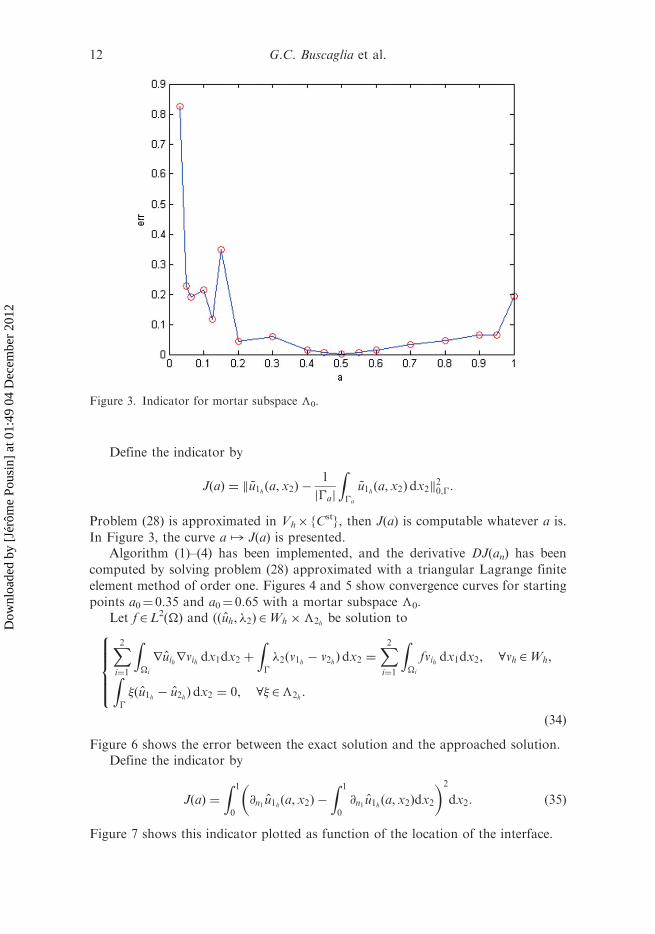
Define the indicator by

JðaÞ ¼ k ~u1hða, x2Þ �1

j�aj

Z�a

~u1hða, x2Þ dx2k20,�:

Problem (28) is approximated in Vh� {Cst}, then J(a) is computable whatever a is.

In Figure 3, the curve a � J(a) is presented.Algorithm (1)–(4) has been implemented, and the derivative DJ(an) has been

computed by solving problem (28) approximated with a triangular Lagrange finite

element method of order one. Figures 4 and 5 show convergence curves for starting

points a0¼ 0.35 and a0¼ 0.65 with a mortar subspace �0.Let f2L2(�) and ððuh, �2Þ 2Wh ��2h be solution to

X2i¼1

Z�i

ruihrvih dx1dx2 þ

Z�

�2ðv1h � v2hÞ dx2 ¼X2i¼1

Z�i

fvih dx1dx2, 8vh 2Wh,Z�

�ðu1h � u2hÞ dx2 ¼ 0, 8�2�2h :

8>>><>>>:

ð34Þ

Figure 6 shows the error between the exact solution and the approached solution.Define the indicator by

JðaÞ ¼

Z 1

0

@n1 u1hða,x2Þ �

Z 1

0

@n1 u1h ða, x2Þdx2

� �2

dx2: ð35Þ

Figure 7 shows this indicator plotted as function of the location of the interface.

Figure 3. Indicator for mortar subspace �0.

12 G.C. Buscaglia et al.

Dow

nloa

ded

by [

Jérô

me

Pous

in]

at 0

1:49

04

Dec

embe

r 20

12

Figure 5. Indicator as function of location of the interface (left) and location as function ofiterations (right).

Figure 4. Indicator as function of location of the interface (left) and position of the interfaceas function of iterations (right).

Figure 6. Error with a mortar subspace �2.

Applicable Analysis 13

Dow

nloa

ded

by [

Jérô

me

Pous

in]

at 0

1:49

04

Dec

embe

r 20

12

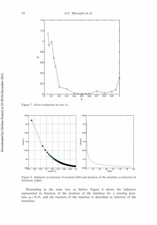
Proceeding in the same way as before, Figure 8 shows the indicatorrepresented as function of the position of the interface for a starting posi-tion a0¼ 0.35, and the location of the interface is described as function of theiterations.

Figure 7. Error evaluation in case �2.

Figure 8. Indicator as function of location (left) and position of the interface as function ofiterations (right).

14 G.C. Buscaglia et al.

Dow

nloa

ded

by [

Jérô

me

Pous

in]

at 0

1:49

04

Dec

embe

r 20

12

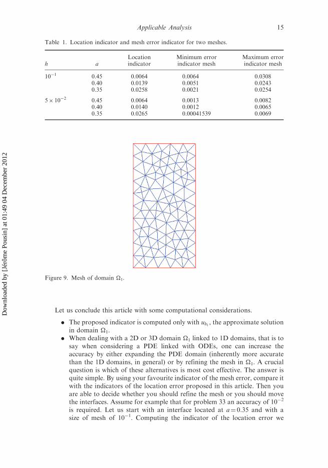
Let us conclude this article with some computational considerations.

. The proposed indicator is computed only with uh1 , the approximate solutionin domain �1.

. When dealing with a 2D or 3D domain �1 linked to 1D domains, that is tosay when considering a PDE linked with ODEs, one can increase theaccuracy by either expanding the PDE domain (inherently more accuratethan the 1D domains, in general) or by refining the mesh in �1. A crucialquestion is which of these alternatives is most cost effective. The answer isquite simple. By using your favourite indicator of the mesh error, compare itwith the indicators of the location error proposed in this article. Then youare able to decide whether you should refine the mesh or you should movethe interfaces. Assume for example that for problem 33 an accuracy of 10�2

is required. Let us start with an interface located at a¼ 0.35 and with asize of mesh of 10�1. Computing the indicator of the location error we

Table 1. Location indicator and mesh error indicator for two meshes.

h aLocationindicator

Minimum errorindicator mesh

Maximum errorindicator mesh

10�1 0.45 0.0064 0.0064 0.03080.40 0.0139 0.0051 0.02430.35 0.0258 0.0021 0.0254

5� 10�2 0.45 0.0064 0.0013 0.00820.40 0.0140 0.0012 0.00650.35 0.0265 0.00041539 0.0069

Figure 9. Mesh of domain �1.

Applicable Analysis 15

Dow

nloa

ded

by [

Jérô

me

Pous

in]

at 0

1:49

04

Dec

embe

r 20

12

get 0.0258, and the indicator of the mesh error is valued between 0.0034 and0.024 (Table 1). Thus the interface is moved to a¼ 0.4 in order to enlarge thesize of the domain �1. The indicator of the location error becomes 0.0139,and the indicator of the mesh error is valued between 0.0051 and 0.0243.The mesh is then refined in the domain �1 with a mesh size of 5� 10�2 andthe indicator of the mesh error is valued between 0.0012 and 0.0065. Theinterface is now moved to a¼ 0.45, the indicator of the location errorbecomes 0.0064. Figure 9 shows the mesh of domain �1. The meshrefinement strategy is quite crude (Figure 10), since the mesh is uniformlyrefined.

. Observe that whatever the values of the indicator of the mesh error is, it ispossible to reach the optimal location of the interface.

References

[1] G.P. Panasenko, Multi-scale Modelling for Structures and Composites, Springer, the

Netherlands, 2005.

[2] J. Leiva, P. Blanco, and G. Buscaglia, Iterative strong coupling of dimensionally

heterogeneous models, Int. J. Numer. Methods Eng. 81 (2009), pp. 1558–1580.[3] P. Blanco, J. Leiva, R. Feijoo, and G. Buscaglia, Black-box decomposition approach for

computational hemodynamics: One-dimensional models, Comput. Methods. Appl. Mech.

Eng. 200 (2010), pp. 1389–1405.

[4] J. Leiva, P. Blanco, and G. Buscaglia, Partitioned analysis for dimensionally-heterogeneous

hydraulic networks, SIAM Multiscale Model. Simul. 9 (2011), pp. 872–903.[5] G.P. Panasenko, Method of asymptotic partial decomposition of a domain, Math. Models

Methods Appl. Sci. 8(1) (1998), pp. 139–156.

Figure 10. Refined mesh of domain �1.

16 G.C. Buscaglia et al.

Dow

nloa

ded

by [

Jérô

me

Pous

in]

at 0

1:49

04

Dec

embe

r 20

12

[6] A. Quarteroni and A. Veneziani, Analysis of a geometrical multiscale model based on the

coupling of PDE’s and ODE’s for blood flow simulations, SIAM J. MMS. 1(2) (2003),

pp. 173–195.[7] F. Fontvielle, G. Panassenko, and J. Pousin, F.E.M. implementation for the asymptotic

partial decomposition, Appl. Anal. 86(5) (2007), pp. 519–536.[8] R. Becker and R. Rannacher, An optimal control approach to a posteriori error estimation

in finite element methods, Acta Numerica, Cambridge, University Press, Great Britain,

2001, pp. 1–102.[9] G. Buscaglia, R. Feijoo, and C. Padra, A posteriori error estimation in sensitivity analysis,

Struct. Multidisciplinary Optimi. 9 (1995), pp. 194–199.[10] G.P. Panasenko, Asymptotic partial decomposition of variational problem, C. R. Acad. Sci.

Paris. Serie IIb 327 (1999), pp. 1185–1190.[11] J.L. Guermont and A. Ern, Element Finis:Theorie, Applications, Mise en Oeuvre, Springer,

Berlin, Allemagne, 2000.[12] F. Fontvielle, Decomposition asymptotique et elements finis, Thesis, INSA de Lyon, Lyon

France, 2004.

Applicable Analysis 17

Dow

nloa

ded

by [

Jérô

me

Pous

in]

at 0

1:49

04

Dec

embe

r 20

12