A Multi-Attribute Tradeoff Analysis for Water Resource ...

A Multi-Attribute Tradeoff Analysis for Water Resource Planning: A Case Study of theMendoza River

by ALLEN JOSEPH CAVICCHI

M.S. Environmental EngineeringTufts University, 1993

B.S. Mechanical EngineeringUniversity of Connecticut, 1987

Submitted to the Department of Electrical Engineering and Computer Sciencein Partial Fulfillment of the Requirements for the Degree of

MASTER OF SCIENCE in TECHNOLOGY AND POLICY

at theMassachusetts Institute of Technology

May 1997

© 1997 Massachusetts Institute of TechnologyAll rights res rved. ,-

Signature of Author

it // ~-.-

Allen J. CavicchiVtJr"lary 7, 1997

ssor Frank E. PerkinsDepartrent of Civil nd nirnmental ineering

Thesis Supervisor

......................................... ........ ...... . .......Dr. Richard D. Tabors

Technology and Policy ProgramA 7 Thesis Reader

Accepted by

Accepted by

OF ~EC--IL '

_.. -3r-ofessor Richard de Neufville/ airm p~ngyxgPicy Program

Professor Arthur •SmithChairman, Committee for Graduate Students

JUL 24 1997-S

Certified by

Certified by

Acknowledgments

I want to acknowledge the great pleasure I had in completing this Thesis under the

guidance of Professor Frank Perkins. The opportunity to travel to Mendoza with Frank, as

well as our regular meetings, allowed me to resolve many curiosities that I had harbored.

Equally I enjoyed the opportunity to work with Dr. Richard Tabors as his support and

encouragement have been a source of motivation. I want to thank my research partner Luis

Paz-Galindo who was always supportive and with whom I had a great trip to Mendoza. I

also want to acknowledge the many people in Mendoza who have worked on the project

and thank them for their hospitality and assistance during my visit in the summer of 1996.

Finally I want to thank my long time friend Peter Janzen who allowed my to use his

computer throughout the execution of this research and the writing of this Thesis.

Table of Contents

Abstract ........................................................................... 6

Chapter 1. Background Information on the Mendoza River Basin and the Multi-Attribute Tradeoff Analysis ................................................. 7

Introduction............. . .............................. ............................... ... 77

Background . ...................................................... .................................... ..... 8

Basis of the Research Effort.......................................................................... . 8

W ater R esource Planning ................................................ .................................. .10

Situation in M endoza ............................................................................................ 12

Departmento General de Irrigaci6n......................................................... 14

Current Problem s ......................................................................... .. 16

Multi-Attribute Trade-Off Analysis (MATA)..............................................................20

Origin and Terminology .................................................................... 20

M A TA in M endoza ............................................................................................. 22

Chapter 2. Irrigation Methodology ............................................................................. 27

Irrigation Technologies ................................................................................... 27

M icro-A spiration..... ............................................................................. 28

D rip Irrigation ......................................................................................... 29

Sprinkler Irrigation................................................................................. 29

System C ost Estim ates ........................................... .......................................... 30

Chapter 3. Water Use Model ................................................................................ 31

D escription of the M odel .............................................................................. 31

Supply ...................................................................................................... . . 31

D em and ............................................................ . . .............................................. 36

Infiltration ................................................ 40

Strategy A nalysis ............................................................................................. ... 43

Analysis Limitations ............................ 4........... ...... 46

M odel O peration ............................................................................................. 47

Chapter 4. Analysis Results ........................................................................................ 48

Chapter 5. Economics of Water in Mendoza and Water Policy Options ......................... 58

Specific Market Failures in Mendoza ............................................... 59

Current Water Charges and Costs .......................................... ........ 60

Ground Water and River Water ........................................ .......... 60

Conjunctive Water Use Supply Costs ..................................... ..... 62

A Price for Water? .................................................................. ......... 63

Will New Irrigation Technologies be Demanded? ............................ ..... 64

Water Management Policy Considerations ....................................... ..... 66

C hapter 6: C onclusions ........................................... ..................................................... 69

B ibliography .............................................................................. ................................... 7 1

A p p en d ix ............................................................................................................................ 7 5

W ater U se M odel .................................................................................................. 76

R esu lts ...................................................................................................... 10 0

Figures and Tables

Figure 1.1: Rivers in the Province of Mendoza, 13

Figure 1.2: Depiction of the Unconfined/Confined Aquifer Division, 18

Figure 1.3: Example Trade-Off Graph, 26

Figure 3.1: Water Use Model Diagram with Dam, 32

Figure 3.2: Water Use Model Diagram without Dam, 33

Figure 3.3: Mendoza River Average Annual Flows, 34

Figure 3.4: Monthly Water Demands and River Water Flows, 35

Figure 3.5: Monthly Crop Water Requirements, 38

Figure 4.1: Trade-Off Graph 1, 52






Tables 1.1: Multi-Attribute Trade-Off Analysis Scenarios, 25

Table 2.1: Pressurized Irrigation System Cost Estimates, 30

Table 3.1: Typical Water Requirements for Various Crops in Mendoza, 38

Table 3.2: Monthly Irrigation Water Demands, 39

Table 3.3: Water Losses in Canals and on Farms, 42

Table 4.1: Futures Analyzed with the Water Use Model, 48

A Multi-Attribute Tradeoff Analysis for Water Resource Planning: A Case Study ofthe Mendoza River

by ALLEN JOSEPH CAVICCHI

Submitted to the Department of Electrical Engineering and Computer Sciencein Partial Fulfillment of the Requirements for the Degree of

MASTER OF SCIENCE in TECHNOLOGY AND POLICY

Abstract

This thesis presents the application of a Multi-Attribute Tradeoff Analysis to thewater resources planning problem associated with the Mendoza river. A conjunctive wateruse model that represents the Mendoza river basin was developed. The model simulates theperformance of several different strategies available for managing both water supply anddemand. More efficient water distribution and improved irrigation technologies arecompared with large infrastructure projects. Relevant attributes are calculated and presentedon tradeoff curves to communicate the performance of different strategies to theorganizations with vested interests. The initial results provide a basis from which a forumcan be created to discuss the water management options available.

The results demonstrate the viability of several structural and non structuralalternatives available to manage the supply and demand for water. Among the latter arethose alternatives that incorporate water conservation and improved efficiency in thedistribution system. These in turn require the development and implementation of policieswhich rectify the economic problems associated with an improperly valued resource. Theeffects of water pricing on farmer behavior are investigated and the results reveal that pricingis feasible. Unfortunately water pricing will not create demand for new irrigationtechnologies, but proper pricing can generate revenues necessary to improve the efficiencyof the distribution system. The results indicate that novel water use policies for the Mendozariver can be beneficial if the responsible agencies commit themselves to work as a team andultimately reach consensus on the implementation of acceptable water managementstrategies.

Thesis Supervisor: Professor Frank E. PerkinsTitle: Professor of Civil and Environmental Engineering

Chapter 1. Background Information on the Mendoza River Basinand the Multi-Attribute Tradeoff Analysis

Introduction

This thesis examines an arid region in northern Mendoza, a Province of Argentina.

The region considered is comprised of the city of Mendoza, several smaller towns, and

agricultural areas. The inhabitants receive their water supply from the Mendoza river. The

Mendoza river primarily supplies water to an agricultural area of between 50,000 and 80,000

hectares. The river also recharges a large ground water aquifer located in the area where

agricultural activities transpire. In response to a drought in the 1960's, farmers in the region

began to pump large quantities of ground water from the aquifer to meet their demands.

Thereafter ground water has been used to supplement river water supplies. Extensive

simultaneous use of surface and ground water has occurred without a suitable conjunctive use

plan or recognition of the renewable capacity of the river basin. Unmanaged use has

exacerbated the contamination of ground water with salt.

Numerous studies have been completed analyzing the economic viability of a dam and

reservoir project proposed on the Mendoza River. Additionally, several studies have been

completed identifying the potential harm that could be created by the construction of a dam

and reservoir. Other regions of the province have experienced notable problems ostensibly

associated with sediment settling in reservoirs leading to increased water infiltration in

irrigation canal distribution systems. Several different organizations have generated reports,

though one organization has control over both the ground water and river water supply. The

controlling organization has polarized its efforts and concentrated solely on a proposed dam

project. The current situation has resulted in an environment where conflict and disagreement

have been insurmountable.

The Mendoza River Basin provides opportunities for the construction of dams. The

river has an average yearly flow of 50 m3/s and flows through a region of the Andes

Mountains where there is substantial elevation change. The river provides water for irrigation,

industry, sewerage, and human consumption in the northern part of the Province of Mendoza.

Various officials in the Province, and at times the national government, suggest that the river

be controlled by the construction of a dam. A dam can provide water regulation enhancements

and additional electricity supply to the region, but the construction of a dam may produce a

number of different problems. Vitally important water and energy policy questions require

evaluation prior to the execution of a large scale project with uncertain costs and benefits.

This thesis examines water management policy options in Mendoza and their impact

on resource consumption. The analysis demonstrates the application of a multi-attribute

tradeoff analysis to the Mendoza River basin. A water use simulation model developed

specifically for the Mendoza River basin calculates parameters associated with water resource

planning problems. (electricity generation, water storage and infiltration, etc.) The capacity of

the system is investigated for different irrigation water demands. The results are displayed

graphically to permit those with vested interests (stakeholders) in Mendoza to examine the

outcomes of different development strategies. These tradeoff graphs provide a basis from

which stakeholders can actively discuss and evaluate the performance of different water

management policies. The results, combined with existing data characterizing farmer

behavior, are utilized to answer the following two questions: (i) Is it possible to establish a

price for water in Mendoza? and (ii) If a price is charged for water will new irrigation

technologies be demanded? The results establish an affirmative answer to the former question

and a negative answer to the latter. Most importantly the analysis reveals the numerous

options available to Mendozans to improve the use of water.

Background

Basis of the Research Effort

The objective of the research in this thesis is to evaluate the future interactions of

water and energy resources in the Province of Mendoza, Republic of Argentina. M.I.T.

executed an agreement with the Universidad Nacional de Cuyo (UNC) and the Provincial

Government of Mendoza which provided a framework for collaborative research projects.

The specific project that provided the impetus for this thesis has been the transfer of the multi-

attribute trade-off (MATA) analysis technique to a research group in Mendoza established for

this project. This was achieved through a demonstration application of the MATA analysis

under the auspices of the project: Evaluacion por Multi-Atributo de los Recursos Hidricos y

Energeticos de Mendoza. (EMARHE)

The project was divided into two components: energy and water. The emphasis on

energy and water for this research effort was a result of several changes in the country of

Argentina. The most significant change was the creation of a wholesale electricity market.

Prior to 1992, the supply of electricity in the country of Argentina was controlled by

government owned and operated organizations. These were referred to as State Society

companies. Between 1989 and 1992 these organizations were privatized through government

sanctioned sales. In conjunction with the privatization process a new framework for the

electricity industry was developed and promulgated.' This framework consists of a wholesalemarket operated by an independent organization with government involvement and

government regulated transmission and distribution companies.

These changes fundamentally restructured the previous methodology that the

government had utilized to plan the future supply of electricity. During several preceding

decades the government owned and operated two state societies: Aqua y Energia and

Hidronor. These organizations coordinated numerous studies throughout Argentina to identify

all possible locations for the development of hydroelectric electricity. While these companies

existed several hydroelectric projects were constructed; as a result, the installed Argentine

electricity capacity is approximately 50% hydroelectric. (Bastos 1993)

In addition to hydroelectric projects constructed primarily to supply electricity, there

have been several facilities constructed in river basins where water is utilized simultaneously

for electricity generation and irrigation. In many river basins the construction of a dam

provides numerous benefits. These benefits may include:

* Electricity generation;

* Intertemporal water storage;

* Tourism;

* Flood control;

* Improved agricultural yields;

* Ground water pumping reductions, etc.

The Province of Mendoza is a region where rivers present the opportunity for multiple benefit

water resource development projects.

The privatization of Agua y Energia and Hidronor substantially changed the way

electricity supply planning occurred in Argentina. The role of the State is now envisioned to

be minimal, while the wholesale market is expected to generate the signals required to

encourage the construction of new facilities. This fact is partly responsible for the Mendozan

interest in examining the interaction of water and energy resources within the framework of

the reformed electricity industry. The evaluation of electricity plants in Mendoza is

complicated by hydroelectric facilities that provide both electricity and irrigation benefits.

The viability of a hydroelectric project is different when compared with a fossil fuel plant.

IArgentine Government, Law 24065, 1992.

The newly established wholesale market represents a source of uncertainty that impacts theplanning process.

To confront this situation two models were developed to evaluate the future provisionof electricity and water use in Mendoza. A model which examines the supply and demand ofelectricity in Mendoza was developed by one investigator at M.I.T. while I developed a

computer model to study water resource planning options on the Mendoza River basin. The

simultaneous use of these models allows the investigation of the future consumption of water

and electricity. Various supply options can be analyzed not only from a financial perspective,

but also as a function of their environmental effects, long run suitability, and performance

when uncertainties are considered.

Water Resource Planning

Examination of pertinent information supplied by Mendozan researchers revealed that

a major element of this research work encompassed water resource planning. The nature of

the effort envisioned here was not as extensive as those executed by others during the 1960's

and 1970's. (Maass et al 1962 and Major et al 1979) The Mendoza river basin has significant

agricultural development in place as result of over 100 years of canal system construction.

The question was therefore not related to examination of numerous sites for both hydroelectric

and irrigation development, but how to utilize the existing system in a fashion which

maximizes the benefits available in the context of the current water supply available and

electricity market framework in Mendoza. To evaluate the situation a model facilitates the

consideration of numerous options available to manage the delivery of water.

The distribution of water in Mendoza is managed by the Departmento General de

Irrigaci6n. (DGI) This organization was established under the constitution of the Province and

enjoys substantial powers in its ability to deliver and regulate the usage of water in the

Province. The DGI is charged with distributing the water from rivers in Mendoza to the land

where crops are cultivated and to the organizations that distribute potable water or have

industrial use permits. The department is also responsible for insuring that farm drainage

networks are functional. During the previous two decades the department has supported the

idea that a dam/reservoir should be constructed on the Mendoza river in order to enhance the

supply of superficial water available during the spring season when river flows are minimal

and irrigation demands are significantly in excess of the flow. (DGI 1970, 1980, 1986)

In addition to the supply of superficial water available to irrigate farms there is a

substantial ground water aquifer available to supplement the river supply when necessary.

The administration of the water extracted from the aquifer is also under the jurisdiction of the

DGI. The existence of two sources of water, combined with the fact that many farmers in theregion have installed ground water pumps, creates a complex situation. The yearly

endowment of the Mendoza river is naturally variable and there exists no guarantee that

adequate supply will be available to satisfy the demand that the DGI is obligated to serve

through supply rights established over several decades. Many farmers have recognized this

potential shortage and have acted individually by installing their own ground water extraction

wells.

These well installations have resulted in changes in the ground water quality and

availability as the farmers are unable to take into account the effects their individual pumping

has on the ground water system. In addition to problems caused by ground water pumping,increased salinity levels have been detected in certain portions of the ground water supply

presumably as a result of extended agricultural activity in the region. This problem is

exacerbated in areas where drainage of excess irrigation water is inadequate. Research work

in Mendoza has revealed high salt concentrations in ground water aquifer layers near the

surface while ground water located at deeper levels has a lower salt concentration. (Alvarez

unpublished 1995) The researchers have reached the conclusion that the salt concentrations in

deeper layers have increased as a result of water transmission between layers. Previously the

deeper aquifer layers had lower salt concentrations. Substantial increases in ground water salt

concentrations have been observed following the installation and operation of numerous wells.

The increased ground water pumping can draw down the free water surface to the point where

the transmisivity between two distinct ground water layers is artificially impacted by the cones

of depression of the ground water wells. Ground water from an upper layer, nearer to the

surface, subsequently mixes with ground water in a layer deeper in the earth.

This exploitation of the ground water, combined with the variability of the flows in the

Mendoza river, results in a situation where water resource planning is critical. To date

planning activities have concentrated on the investigation of the installation of a dam on the

Mendoza river. The potential for multiple benefits exist. An important element of this thesis

is the modeling of water resources in this region in order to compare the benefits of several

different potential projects. The viability of the water projects that generate electricity is

important. Hydroelectric projects can be compared with other electricity sources in order to

examine the costs and benefits of both sources of electricity supply. The multiple benefit

nature of a hydro-project requires an extensive analysis when contrasted with a fossil fuel

facility.

The model also permits the investigation of other methods of improving the supply of

water. A planned conjunctive use is envisioned with the model. The recharge of the

11

unconfined aquifer is compared with the volume of ground water pumping required. A globalwater balance is calculated to evaluate the conjunctive water use. Ground water pumpingbatteries are planned in regions where water with low salt concentrations exist. The batteriescan replace supplies potentially available from a reservoir while allowing improvements inproblem areas to commence.

Equally important is the mitigation of losses in the water distribution system and the

potential for improved usage at the farm level. The distribution system is comprised of

numerous earthen canals and the primary technique employed for application is gravity

distribution. This system supplies a much larger quantity of water than is required to achieve

effective irrigation of the land in question. The current method of distributing the water does

not take into account the exact quantity a farm may require, but is delivered on the basis of

legal rights to the water whether it is needed or not. This can create substantial waste as there

exists no mechanism to equate the supply with demand or to provide an incentive for reduced

levels of use. A means of countering this problem is explored through the potential

application of water pricing which reflects its opportunity cost. This is a central issue in this

thesis as the question posed is whether a water usage policy, including pricing based on

scarcity, would modify consumptive patterns sufficiently to materially assist in managing the

long term water supply for Mendoza?

Through the use of a simple simulation model the impacts of improved supply

management with large and small scale projects is studied. Equally the positive effect of

demand management is explored to permit a fair comparison of the options available.

Combinations of various projects are analyzed to explore the alternatives. The objective of

insuring a guaranteed supply of water is envisioned throughout the analysis. Policies that

could be exercised by the DGI are proposed as a means of achieving the desired goal of a low

cost, properly employed source of water for the region.

Situation in Mendoza

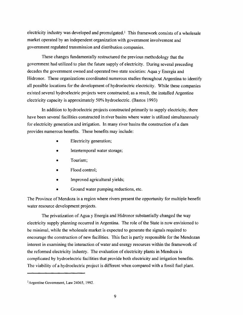
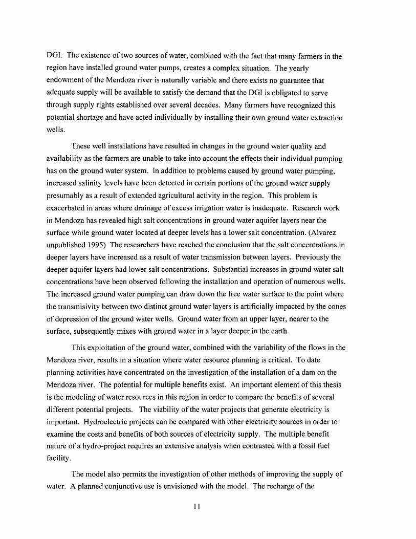
There are four significant rivers in Mendoza whose water is distributed by the DGI.

(see Figure 1.1) The Mendoza and Tunuyan rivers which are located in the north, and the

Diamante and Atuel rivers located just south of the center of the Province. The Diamante and

Atuel rivers have several man-made works. The focus of the research in this thesis is on the

Mendoza river, but it is beneficial to discuss other experiences elsewhere in the province as

many relevant concerns result from previous river basin developments.

The current state of affairs in Mendoza is complex and results from more than 100

years of agricultural development in the region. In order to familiarize one with the water use

12

/i /r 0 V / A/ C / 4 4

SA A./ J . A. AJ

/V C/A

OZA>4 KK

Source: CRAS ". ,." Z

'I

/ A C / -/,r'.4 Al1 F - ,LAr

(J-.4.A

Fig•re 1.: Rivers i. the Province of Medea

IT

I

k

\

zI

t=;

tp

'$:

issues in the region a brief discussion of pertinent matters is presented. The first issue relatesto the administration of water in the region. This is followed by examples of water workspreviously constructed in Mendoza to control the distribution of water. The concluding

portion relates to the effects of large scale water diversion and distribution on the local

environment.

Departmento General de Irrigaci6n

The DGI is charged with the distribution of water to all users. This responsibility

includes operation and maintenance of the entire water distribution system for the Province of

Mendoza.

The DGI operates as a function of their establishment by the provincial constitution,law #322 and the Water Law of 1884.2 The structure and hierarchy are defined by the

constitution. The structure contains the following elements: appeals council; administrative

commission; superintendent; water sub delegations; honorary assemblies; and the irrigation

channel inspection group. The primary power of the DGI is vested in the superintendent. The

responsibilities of the superintendent are defined by Provincial Law and Articles 3 and 6 of

Law # 322.. These functions are the following:

* Administer the water of the Province;

* Exercise police powers when investigations are necessary relating to the water supply, the

natural river channels, river banks, and service zones;

* Dictate all measures necessary to insure effective use and realization of benefits from the

resource;

* Resolve administrative questions that arise due to the distribution of the water, drainage,

or staff;

* Respond to complaints and claims made against employees of the DGI;

* Establish the distribution allotments in times when water is scarce;

* Impose sanctions on those who violate the prescriptions of the Water Law. These

sanctions can be a simple fine and elevate to a revocation of the right to the water;

* Understand all original paperwork associated with applications for concessions for

irrigation, industrial, and energy rights;

2Constitucion de la Provincia de Mendoza, Ley General de Aguas, 1884, Ley No. 322.

Know about appeals and in final instances the resolutions of the sub delegates of water andthe inspectors where sub delegations do not exist.

The sub delegates are organizationally beneath the superintendent and are in charge of

the administration of each particular river, carrying out the same functions in their respective

regions; the equitable distribution of water for irrigation and remaining uses. These groups are

responsible for the governing, administration, and policing of water in their respective

jurisdiction. They have responsibility for direction and control of the diversion works and the

canal systems. Additionally, they are in charge of administrative paperwork and accounting in

their region as well as the implementation of small projects that modify elements of the

distribution system. They are permitted to modify rights to the water in times of emergency or

danger.

The Honorary Assemblies of Irrigators collaborate with the sub delegations to obtain

optimum management of the river water and to achieve a smooth interaction amongst

irrigators in each jurisdiction. The assembly consists of the Sub delegate, a zone advisor, and

three irrigators elected to the assembly of inspectors. Their functions are limited to the

advising and supervision of the workings of the irrigation works, drainage, and the cleaning

and conservation of the canals as well as suggesting when canal lining is desirable. The intent

should always be to improve the distribution and utilization of the water.

The final group, Inspectors of the channels, is responsible for the physical operation of

the system. Their responsibilities include the operation of the canal system insuring proper

distribution of water, administration of funds resulting from fines, payment of staff who clean

and maintain the works, and financing of small projects. They are also permitted to adjudicate

conflicts between users up to the point where the problem does not extend beyond 300

hectares. The election of these authorities is determined by the Laws # 2503 and 322. This

group has several responsibilities and its function is a primary component of the decentralized

management structure of the DGI.

These groups comprise the structure responsible for the management of the water

distribution system. The creation of the DGI under the provincial constitution gives the

organization substantial autonomy. Historic data indicate that the department has

implemented few substantial capital projects during the most recent 25 years. (Braceli 1985)

The importance of this organization in relation to this thesis is the fact that any policies

developed for the improvement of water supply would be implemented by the DGI. Their

history and administrative capacity must be carefully considered when proposing any water

management policies.

Current Problems

Several administrative and physical problems have been identified by National andMendozan agencies including: El Instituto Nacional de Ciencia y T6chnica Hidricas

(INCYTH), El Centro de Economia, Legislaci6n y Administraci6n del Agua y del Ambiente

(CELAA) and El Centro Regional de Agua Subterrinea. (C.R.A.S.) A listing of several issuesis as follows:

* The water rights system utilized in Mendoza insures the delivery of water to those with

rights regardless of whether the water is actually utilized. The system is not regularly

updated though significant information exists which indicates that several thousand

hectares registered to receive water are not cultivated. This excess delivery reduces the

supply available to those who could utilize it and exacerbates salinization problems.

* The lack of attention given to conjunctive use of ground water and surface water has

perpetuated continued pumping of ground water. The result has been worsened

salinization problems in the ground water aquifer. The DGI has prevented continued

ground water extraction in certain regions, but this adversely affects farmers who do not

receive their river water supply.

* Those people with rights to the water have no guarantee that water will be delivered due to

seasonal and yearly stream flow variations. Many have acted individually and installed

ground water pumps to insure an adequate supply. These actions have not been managed

in conjunction with an understanding of the entire surface/subsurface water system.

* Few capital projects to reduce losses and improve use have been implemented.

* Enhanced ability to supply water from the river year round with a reservoir seems to have

been emphasized with little attention given to supply management options.

* Many alternatives have been proposed, but few studies exist analyzing the potential

improvements. This situation has been identified previously by Frederick in 1975.

Currently the Mendoza region has experienced two significant physical problems. The

first problem is elevated salt concentrations in the ground water. The second problem arises

due to the settling of sediment in a reservoir. Elaboration on each of these issues provides

insight into the benefits that the formulation of an overall conjunctive use plan can provide to

preclude future difficulties.

16

A problem associated with irrigation is that ground water salt concentrations tend torise due to repeated application of water to the land. The river water salt concentrations vary

between 500-1500 micromho/cm while concentrations as high as 5500 micromho/cm have

been measured in the ground water. (Alvarez unpublished 1995) This problem has become

more pronounced during the most recent twenty years due to increased exploitation of the

ground water which has caused interaction between upper levels of ground water and levels

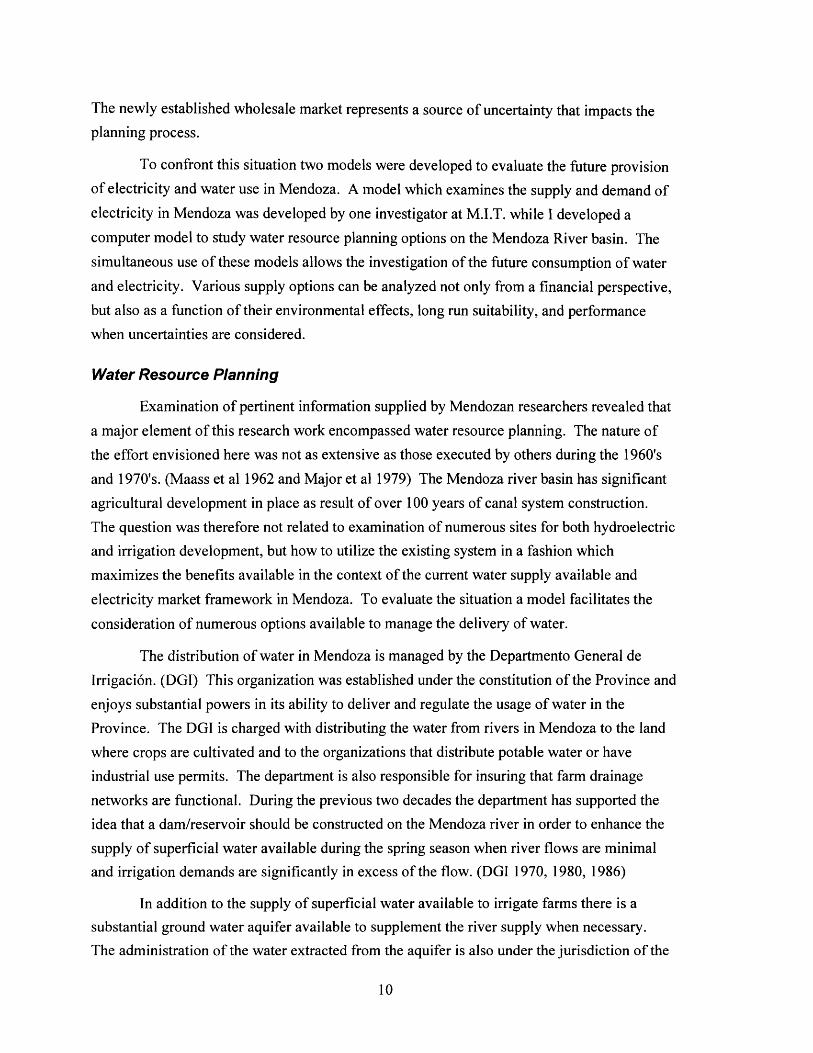
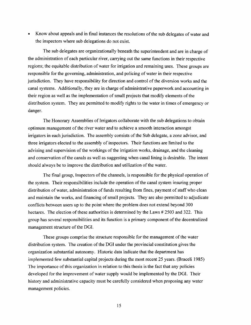
located deeper in the earth. The region in question has two distinct ground water aquifers.

The first is an unconfined aquifer located south west of the City of Mendoza. The second is a

multi-layered, confined aquifer located north east of the City of Mendoza. (see Figure 1.2)

The geology of the region creates these two distinctly different regions. The organization that

has studied this area most significantly is the Centro Regional de Agua Subterranea. (CRAS)

This group has generated numerous data which verify the existence of the two different

ground water aquifer areas. The confined area contains at least three lenses of low

permeability material that provide containment of water at substantial piezometric heads. The

water quality in each of these regions has been monitored extensively and the increased salt

concentrations have been observed in numerous locations.

Level I is the water located nearest to the surface (0-80 m), the second is between 80-

200 m, and the third occurs at depths greater than 200 m. Elevated levels of salt in the ground

water have been observed in the upper two levels while the third continues to be affected only

minimally. In certain regions observations of considerable interaction between the upper level

and the second level have been attributed to extensive ground water extraction in a region

where the transmisivity between levels is relatively high. Exacerbating this situation has been

the poor installation of numerous wells. These wells have casings that are known to leak due

to corrosion of the materials used for construction of the wells and thereby transmit water

between levels. The upper level has experienced serious elevations in the concentrations of

salt in the water which is the result of extensive irrigation. This phenomena is observed in

many regions throughout the world where irrigation continues for decades.

The second problem discussed commonly in Mendoza is a problem referred to as

"Aguas Claras." Defined literally this term signifies "clear water" and involves the following

phenomena: (i) sediment in the reservoir water settles to the bottom, (ii) water released from

the reservoir has an increased capacity to transport sediment, (iii) the water enters unlined

irrigation canals and carries away sediment accumulated in the canal, (iv) the rate of

infiltration in the canal system rises, (v) the free surface of the ground water rises flooding

irrigable land. This phenomenon has been observed in other parts of Argentina following the

construction of dams.

17

**1~~~'P-H "t.sPAIAii.)S

b4r!

sd

•

.4ev.

GRAIA U(ENOOZL

G.Cd-abrnua 2 P2.3 t.Wawar&a m Uhnm

('p~

'p'7c.OCH lAS

% ll,

LAkIA U

;;I

I

r

rrr

It

I i i

rr

,,,,,

- -- I

,,r,

"M 1SORO

021

CRcrc2La(.

C

mE

Ce14

The clear water problem is an important issue when considering the potential

construction of a dam/reservoir in a location near the city of Mendoza referred to as

Potrerillos. There is significant uncertainty associated with the quantification of the effects of

clear water. CELA, INCYTH, and CRAS believe that the lining of several irrigation canals is

necessary to combat this problem and limit infiltration. This problem is not treated explicitly

in this thesis for the following reasons: (i) an accurate quantification of the problem does not

exist, (ii) the exact cause of the problem has not yet been verified, (iii) mitigation of the

increased infiltration requires lining of unlined canals and increases the cost of a dam/reservoir

project substantially.

The increased costs of a dam/reservoir project reduce its economic viability

considerably. Lack of inclusion of the clear water problem with a dam project creates more

favorable results. The initial work presented in this thesis intends to demonstrate the tradeoff

analysis and identify feasible water management strategies. To date numerous options have

not been considered in Mendoza, nor has the critical requirement that conjunctive use of

ground water and surface water be managed together. The results indicate that, of several

projects examined to improve the supply of water to the farms, a large scale project has

significantly higher risks with benefits that rely on uncertain forecasts. The clear water

problem adds to the uncertainty. If a dam/reservoir project is part of the final set of interesting

options then a more detailed analysis can be executed to attempt to precisely integrate the

clear water problem.

Multi-Attribute Trade-Off Analysis (MATA)

Origin and Terminology

The past 25 years demonstrate the DGI's continued insistence that a multi-benefit dam

project is the optimal solution to Mendozan water management problems. (DGI 1970, 1980,1986) The DGI analyses consistently ignore other viable alternatives for water management.

Other concerned agencies have identified and characterized potential problems associated with

the construction of a dam, but no attempt has been made to unite interested parties in a forum

that permits a thorough discussion of alternatives. The utilization of an open planning process

presents the opportunity of identifying strategies for water management that are acceptable to

each stakeholder.

Previous analyses executed by the DGI in Mendoza have focused on the construction

of a dam in the town of Potrerillos. There seem to be several reasons to explain this emphasis.

The multiple benefits available from a dam/reservoir project motivate the overwhelming

interest. These multiple benefits include:

* Electricity generation;

* Water storage to meet irrigation demands;

* Flood control;

* Tourism;

* Potential improved agricultural production;

* Ground water pumping reductions, etc.

Additionally, a large infrastructure project provides jobs for the unemployed and tends

to enhance the local economy during construction. Equally a dam project has risks. The clear

water problem defined previously is a serious concern which is not well understood. Other

environmental impacts will result when the tourism developments are initiated and increased

numbers of people frequent the area.

The inability of all stakeholders to reach consensus on the effectiveness of a dam has

been a problem. The rapid privatization of the electricity market in Argentina removed the

emphasis on state led planning for electricity supply and forced provinces to carefully assess

their local conditions. This renewed interest has presented the opportunity to formulate a

MATA to analyze the problem.

The use of a MATA to assist in understanding the available alternatives presents anopportunity to examine the outcomes of numerous water management improvement strategies.The development of an effective long term strategy demands a multiple-issue, multiple-option

planning framework which the MATA analysis offers. The complexity, controversy, and

uncertainty inherent in large scale water resource system development has clearly been a

primary reason for the paralysis evidenced in Mendoza: no substantial modifications have

been implemented for 25 years though numerous problems have been identified. The MATA

analysis is utilized here to demonstrate the outcomes of different infrastructure developments

and to provide a forum for productive debate.

A succinct description of this analysis is given by Andrews 1990:

"Scenario-based multi-attribute tradeoff analysis is a technique that allows

negotiating parties to observe the performance of strategies, the effects of uncertainty,and the interactions among components of a complex system in multi-attribute space.

This helps the group to invent better strategies having more of the characteristics that

each party prefers, thus improving the potential for consensus. By involving the

parties in the analysis, their creativity is harnessed, a shared understanding of both

issues and options grows, and the results are more likely to be accepted by the group.

The analyst plays a non-traditional role in facilitating the joint fact-finding effort

among the parties."

The elements utilized to implement this methodology were initially outlined in work

completed by Merrill and Schweppe (1984) and Geraghty, Lethrop and Merrill, et al (1984).

This work developed as a result of placing emphasis on the choice of strategies in an open

decision environment and the explicit analysis of various tradeoffs considering a wide range of

uncertainty. These authors described a Multi-Objective Decision Analysis technique in which

scenarios are conceived through the combinations of options (strategies) and uncertainties.

The results are evaluated using decision analysis techniques and linear programming

algorithms. The terms defined for describing the components of the analysis are as follows:

Strategies (options): A strategy represents a decision over which the parties have

control and which can be implemented. These represent types of projects that can be

either combined or solely executed to achieve water usage planning objectives. 3

3A combination of distinct projects can represent a strategy or a single project can equally represent a strategy.

The defined strategies shown in Tables 1.1 & 1.2 show the projects associated with a strategy. I use the words

strategy and project interchangeably in many instances.

Uncertainties: An uncertainty is an event over which the parties do not have control.

Uncertainties represent demand forecasts, stream flow variances, economic variationsetc.

Scenarios: A scenario is a combination of a strategy with a set of uncertainties. Ascenario is then evaluated using applicable analysis techniques.

Attributes: An attribute is a measure of the performance of a strategy. Attributes are

defined by the stakeholders and utilized in assessing the merits or outcomes of a

scenario's simulation.

The MATA retains the describing function defined by Merrill and Schweppe using

strategies (options), uncertainties and attributes, though it eliminates the optimization

algorithms from the analysis technique. This permits the technique to be more readily applied

in an open decision environment. In the tradeoff analysis, computer simulation is used to

analyze scenarios. Results are displayed graphically to identify inferior strategies and to assist

in identifying reasonable compromises.

MATA in Mendoza

The planning of water use in Mendoza presents multiple attributes which provide a

forum for productive interactions among the stakeholders. The MATA technique is useful in

this situation where multiple attributes are definable and several investment strategies have

been proposed though no effective means of analyzing these strategies has been formulated.

Numerous stakeholders exist and notable conflict is apparent. Furthermore, there is a

substantial amount of uncertainty in future forecasts which include both water demand

variations and variable stream flows.

The use of the MATA envisions the identification of all attributes of interest prior to

commencement of the analysis. When vital attributes are identified one develops several

different scenarios which combine investment strategies with various futures. Each of these

scenarios is analyzed and the values of the attributes associated with them are displayed

graphically. Unfortunately the DGI was not involved in the attribute definition and model

development which are a part of the study reported on herein. Attributes were defined with

the Mendozan research group and follow-up analysis will be necessary when the DGI

involvement increases.

A water use simulation model is utilized to provide quantified values for the attributes.

Trade-off graphs are constructed and provide a means by which the results of the analysis can

be discussed amongst the constituencies interested in the strategies under consideration. The

/

graphic displays are plots of attributes in two dimensional space. This permits one to display

significant features of the project in a fashion where people can easily understand their

relevance. Attributes selected initially for this study are the following:

* Average quantity of ground water pumped calculated over a 25 year period 4;

* Electricity generated by facilities existing or proposed ;

* Quantity of water that recharges the unconfined aquifer;

* Quantity of water that infiltrates on the farms;

* Electricity consumed to pump ground water;

* Economic benefits associated with dam/reservoir projects;

* Present value costs of scenarios;

* Internal rates of return for scenarios;

* Net present values.

One important attribute related to water resource planning has not been considered.

Typically in a water resource analysis one examines the ability to meet demand in each period.

Penalties are conceived when the system is incapable of satisfying the water requirements.

The initial analysis executed for the Mendoza river assumes that the demand is always

satisfied with a combination of surface water and ground water and thus no penalties for

failure to meet demand are considered. The analysis can be broadened to include scenarios

that make greater demands on the water supply such that the ground water is mined. The

analysis presented in this thesis demonstrates the initial application of the MATA and the fact

that a conjunctive use can be planned for the water resource. A more extensive analysis can

be developed utilizing this initial work as its basis

Changes in the values of the attributes are examined under several different futures by

analyzing the scenarios with the water usage model. Table 1.1 provides examples of strategies

and futures combined into scenarios as well as example results that provide values for some of

the relevant attributes. A brief explanation of the key elements of the strategies is as follows:

0. Construction of a dam at Potrerillos with a useful reservoir capacity of 250 hm 3.

1. Construction of a dam at Potrerillos with a useful reservoir capacity of 500 hm 3.

4The 25 year period was identified by the Mendozan research group as the time period of interest.

2. Construction of a dam at Potrerillos with a useful reservoir capacity of 250 hm 3 and an

assumed increase in infiltration due to clear water of 15 %

3. Construction of a dam at Potrerillos with a useful reservoir capacity of 250 hm 3 and an

assumed increase in infiltration due to clear water of 30 %

4. Construction of a dam at Potrerillos with a useful reservoir capacity of 250 hm 3 and

construction of the marginal canal.5

5. Construction of the marginal canal.

6. Construction of the marginal canal and an enlargement of the electricity generation facility

at Condarco.

7. Construction of the marginal canal and a reduction in canal losses of 12 %.

8. Construction of the marginal canal and a reduction in canal losses of 24 %.

9. 24 % reduction in canal losses.

10. 12 % reduction in canal losses.

11. 12 % reduction in canal losses and 10 % loss reduction on farms.

12. Scenario 11 with Construction of the marginal canal

An example of a tradeoff graph is presented in Figure 1.3 to illustrate the process in

which one compares the attributes resulting from the analysis of numerous scenarios. In

Figure 1.3 a graph of two attributes is presented. The present value costs of each strategy

analyzed for future #1 are plotted versus the average yearly volume of ground water pumped

during the 25 year analysis period. The MATA is characterized by studying the values of the

relevant attributes plotted in this two dimensional space. The axes are designed so that the

origin represents the most desirable location for a point to be located. As points move away

from the origin, in either direction, there is a worsening of the performance of one or both

attributes. The interpretation of the performance of one scenario compared with anotherinvolves drawing a vertical and horizontal line from each point in a direction that represents a

degradation of the attribute. Any point that lies above and to the right, within the box defined

by the vertical and horizontal lines, is considered inferior when compared with the point from

which the lines are drawn. For example, in Figure 1.3 a vertical and horizontal line are drawn

from scenario 8 to illustrate the dominance of 8 over scenarios 6, 11, and 12.

5The marginal canal is a proposed project that would remove water from the river at Condarco and transport it to

Cipolletti. This canal eliminates the infiltration in this tract of the river.

Table 1.1: Multi-Attribute Trade-Off Analysis Scenarios

Scenarios ConsfidredrforManaging the Supply and Distribution of Water (1996-2021)

Strategy Water Demand Variations Water Loss VariationsPotable (OSM) Industnrial Irrigation Canal Marginal Canal Lining Aguas Glaras Improved

(Clear Water) Usagexisting Cach/Con b695 Forecast Constant 74,500u hectares No No No No

rrangement)Potrerillos 6/95 Forecast Constant 74,500 hectares No No No No)Potrerillos w/ 500hm3 Util. 6/95 Forecast Constant 74,500 hectares o No o No)Potrerillos w/clear water 6/9 Forecast Constant 74,500 hectare No Yes Yes (15%) No5%))Potrerillos w/clear water 6/95 Forecast Constant 74,500 hectares No Yes Yes (30%) No0%)) Potrerillos w/ Marginal 6/9 Forecast Constant 74,500 hectares Yes No No Noanal) Marginal Canal 6/95 Forecast Constant 74,500 hectares Yes No No No) Marginal Canal with 6/95 Forecast Constant 74,500 hectares Yes No No Nonlarged Condarco) Marginal Canal plus 12% 6/95 Forecast Constant 74,500 hectares Yes Yes (12%) No Noeduction in Canal Losses) Marginal Canal plus 24% 6/95 Forecast Constant 74,500 hectares Yes Yes (24%) NoNoeduction in Canal Losses) 24% Loss Reduction in 6/95 Forecast Constant 74,500 hectares No Yes (24%) Noanals0.) 12% Loss Reduction in 6/95 Forecast onstant 74,500 hectares No Yes (12%) No Noanals1.) Existing w/12% + 10% 6/95 Forecast Constant 74,500 hectares No Yes (12%) No Yes (10%)oss Reduction vs. existingach/Con2.) Existing w/MC+ 12% + 6/95 Forecast Constant 74,00 hectares Yes Yes (12%) No Yes (10%)D% Loss Reduction vs.xisting Cach/Conotes: 1) Estimates of impact of clear water problem are ARI I ARY and are offset by loss reductions through canal lining and/or marginal canal;

knowns: xtent and exact cause of the clear water problem; Historical variations in the free surface groundwater level in the area of the farms;Accurate estimates of canal losses for a full year. I I

Scenarios Considered for Managing the supply ancid Distribution of Water (1996-2021)

Scenario Pertinent Results Compiled From Multiple Model RunsTotal Quan. of Total Infnitration (hm3) Ave.quan.of (Uw Ave. quan. or total cost

GW Pmpd(hm3) Farms/Canals Cach-CIp pumped (hm3tyr) Elec. (Gwhlyr) PV ($000)xisting (;acn/h;on 4682.11 6935.95 !5170.8rrangement 187.28 245.84 N.A.Potre-nllos 2419.8 6935.95 251.17 96.79 876.17 238,862) Potrerillos w/ 500hm3 Util. 1575.67 693.95 273.81 63.03 938.8 360,36)Potrenllos w/clear water 2658.4 6935.95 6023.13 106.34 877.56 241,5595%)) Potr-eirios-wclear -water 6935.95 6789.8116.9 879.5 244,9190%)) Potrellos w/ Marginal 1443.39 6935.95 1774.58 57.74 861 247,711anal

) Marginal Canal with 3774.8 693.95 2531.68 150.99 304.52 62,227nlarged Condarco) Marginal Canal plus 12% 3442.55 6T59.12 3142.72 137.7 245.84 27,067eduction in Canal Losses) Marginal Canal plus 24% 3088.23 5278.26 3142.72 123.53 245.84 30,427eduction in Canal Losses) 24% Loss Reduction in 3903.6 5278.26 5170.75 156.14 245.14 21,578anals3.) 12% Loss Reduction in 4308.5 6159.1 5170.75 172.34 245.84 18212anals1.) Existing w/12% + 10% 3989 5465.5 5170.75 19. 245.84 96,393,ss Reduction vs. existingach/Con.) Existing w/MC+ 12% + 3162.25 5465.5 3142.72 126.49 245.84)% Loss Reduction vs.xisting Cach/Con

Total Demand 22908(hm3)

i- - - - -

A frontier is defined by the points located nearest to the attribute axes. These pointsdo not strictly dominate each other and represent those scenarios where there are tradeoffsbetween attributes. The selection of the most suitable strategy occurs through an opendecision-making process in which a group of stakeholders examine the results together and

discuss the impacts of the tradeoffs depicted by the graphs. Several tradeoff graphs are

generated to permit an examination of the performance of the different attributes. Scenariosthat consistently are located on the frontier, when compared with other attributes, are those

that form the potential group that stakeholders consider. Inferior scenarios are subsequently

eliminated.

lue Costs vs. Average Quantity of Ground Water Pun

.1

*4 *0 .2 .3

* 12

.8 *7

3.00 60.00 80.00 100.00 120.00 140.

Ave. Quantity of Ground Water Pumped (hm3/yr)

Figure 1.3: Example Trade-Off Graph

Scenarios that consistently yield desirable results are considered "robust." The

stakeholder group then determines whether better scenarios can be invented and, if so, these

are then analyzed and added to the graphs. The analysis presented in this thesis constitutes the

first step in the tradeoff analysis. With the assistance of the Mendozan team 13 strategies and

5 futures were identified for this initial analysis. The continued definition of strategies and

futures would comprise the next activity in the MATA. Those new scenarios would then be

analyzed to determine if they represent better solutions.

Chapter 2. Irrigation Methodology

The primary method of irrigation used in Mendoza is distribution of water by gravity.The water is applied to the fields either in furrows or by flooding. This method of waterdistribution typically results in an efficiency of 60 to 70 percent, indicating that 60 to 70percent of the water applied to the field is used by the crop for evapotranspiration while 30 to40 percent is lost. Losses are characterized by either deep percolation into the soil at the rootzone or runoff from the field. In this thesis the lost water is not considered available forirrigation. The water that percolates into the soil ultimately mixes with water at an elevatedsalt concentration. This ground water located near to the surface of the land has high saltconcentrations and is unable to be utilized for irrigation. Water that runs off the field is alsounavailable for use. This water either infiltrates into the contaminated upper layer of groundwater or evaporates. There is no evidence that excess water returns to the river. The waterlosses on the fields can be reduced through the use of modem irrigation technologies for theapplication of irrigation water.

Modern irrigation technologies achieve an application efficiency of 85 to 100 percent.(Verplancke 1992) The highest efficiencies can be obtained from a drip irrigation system.Significant improvements can also be realized utilizing a sprinkler or aspiration system. Thestrategies analyzed in the water usage model that envision improved use assume the utilizationof these modern irrigation technologies. A conservative estimate of the reduction in losses ismade to represent the additional water available through improved application. Reasonableestimates of the capital costs of new systems are employed. The technologies considered arecurrently available in Mendoza and the capacity to install and operate the systems correctly isconsidered in the implementation of the policies.

Irrigation Technologies

The province of Mendoza has investigated and applied several types of pressurizedirrigation technologies which deliver water to the plants more efficiently. The primaryobjective is to accurately estimate the quantity of water demanded by the crop being irrigatedand to deliver a quantity of water that just meets this demand. The methodology requiresestimates of the crop demand and a thorough knowledge of the physical characteristics of theirrigation technology considered. A suitable system design is developed as a function of thequantity of land requiring irrigation. The vital element for insuring success of these systems isthe ability of the farmers to operate them effectively. Pressurized irrigation systems areexamined in the water use model as a means to improve the efficiency of water use whilesimultaneously conserving the supply.

Three different systems have already been implemented on a limited scale inMendoza: sprinkler systems, micro-aspiration, and drip irrigation. The systems utilizepressurized water with the major differences being the method of delivery of the water and thedistribution system required. A description of the requirements of each of these systems andan estimate of the installation and operational costs were obtained from actual experiences inthe Province of Mendoza.

Micro-Aspiration

Micro-aspiration is a system that provides small volumes of irrigation water to thecrops. The water is emitted as a spray over an area of between 3-7.5 meters in diameter. Theprimary components of the system are the following: pump and filtration element, pressurecontrol device, principal and secondary water distribution networks, lateral delivery piping,and spray nozzles.

The pump extracts water from either a collection pond, a tank or a ground water well.The appropriate design of the water collection source is a function of the property beingirrigated The discharge pressure is monitored and adjusted to insure proper operation of thesystem as a function of the demand. This control system permits flow and pressure regulationand compensates for any losses in the filtration elements. After the water flows through thepump/filter/control system it is delivered to the distribution network. The primary andsecondary distribution network deliver the water to smaller lateral piping. These smaller pipescontain spray nozzles that atomize the water and apply it to the crops.

The spray nozzles can have moving parts or consist of only a nozzle. The precisequantity of distribution elements depends on the type of crop irrigated. The spray nozzles canbe obtained with a pressure control that permits constant flow above a specified inlet pressure.Typically the nozzles are not equipped with pressure controls and the flow varies as a functionof the system design.

The application of this system demands careful attention to the design parameters.The operational costs can vary significantly if the system is designed incorrectly. Theextensive water distribution network creates frictional losses. These losses, in combinationwith the nozzle pressure requirements and filter specifications, must be analyzed properly toselect an adequate pump. Frictional losses in the piping can be considerable if piping isimproperly sized. Errors can increase the operational costs of the system considerably. Thissituation must be specifically analyzed as a function of the area that will be irrigated.

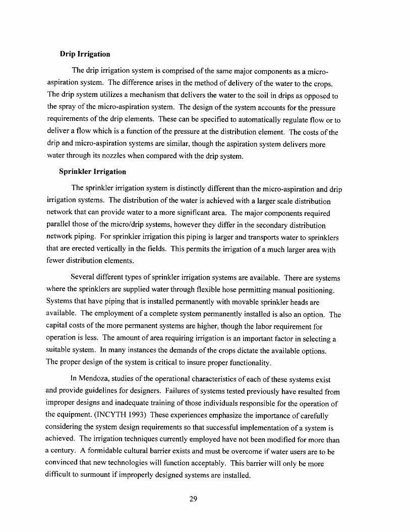
Drip Irrigation

The drip irrigation system is comprised of the same major components as a micro-aspiration system. The difference arises in the method of delivery of the water to the crops.The drip system utilizes a mechanism that delivers the water to the soil in drips as opposed tothe spray of the micro-aspiration system. The design of the system accounts for the pressurerequirements of the drip elements. These can be specified to automatically regulate flow or todeliver a flow which is a function of the pressure at the distribution element. The costs of thedrip and micro-aspiration systems are similar, though the aspiration system delivers morewater through its nozzles when compared with the drip system.

Sprinkler Irrigation

The sprinkler irrigation system is distinctly different than the micro-aspiration and dripirrigation systems. The distribution of the water is achieved with a larger scale distributionnetwork that can provide water to a more significant area. The major components requiredparallel those of the micro/drip systems, however they differ in the secondary distributionnetwork piping. For sprinkler irrigation this piping is larger and transports water to sprinklersthat are erected vertically in the fields. This permits the irrigation of a much larger area withfewer distribution elements.

Several different types of sprinkler irrigation systems are available. There are systemswhere the sprinklers are supplied water through flexible hose permitting manual positioning.Systems that have piping that is installed permanently with movable sprinkler heads areavailable. The employment of a complete system permanently installed is also an option. Thecapital costs of the more permanent systems are higher, though the labor requirement foroperation is less. The amount of area requiring irrigation is an important factor in selecting asuitable system. In many instances the demands of the crops dictate the available options.The proper design of the system is critical to insure proper functionality.

In Mendoza, studies of the operational characteristics of each of these systems existand provide guidelines for designers. Failures of systems tested previously have resulted fromimproper designs and inadequate training of those individuals responsible for the operation ofthe equipment. (INCYTH 1993) These experiences emphasize the importance of carefullyconsidering the system design requirements so that successful implementation of a system isachieved. The irrigation techniques currently employed have not been modified for more thana century. A formidable cultural barrier exists and must be overcome if water users are to beconvinced that new technologies will function acceptably. This barrier will only be moredifficult to surmount if improperly designed systems are installed.

System Cost Estimates

The costs of previously installed pressurized irrigation systems in the provinces ofMendoza and San Juan provide a basis for the cost estimates utilized in the analysis. The dataare shown in Table 2.1.

Table 2.1: Pressurized Irrigation System Cost Estimates

Source: Instituto Nacional de Ciencia y T6chnica Hidricas, Seminario Nacional de RiegoPresurizado, Centro Regional Andino, Mendoza, Argentina 1993.

The figures presented in Table 2.1 are obtained from distinct experiences orpreliminary estimates available in Mendoza. These values should not be considered highlyaccurate, but only representative of the level of costs associated with the implementation ofthe technologies investigated. The costs can vary considerably as a function of specificcircumstances. For example, the applicable electricity tariff affects the operational costsignificantly. The operational cost differences shown are derived from electricity tariffsbetween .03 and .085 $/kwh. Equally the installation of the pumping system can affect costsconsiderably. If a system employs a ground water pump the costs are lower when compared tothe extensive development required to install a system that utilizes water provided from acanal system. In the latter case a storage facility is required to permit proper pump operation.

The installation of pressurized irrigation systems results in a more efficient use of thewater. (Verplancke 1992) This improved utilization permits conservation of the availablesupply by applying a volume of water that is commensurate with the crop requirement. Thepotential improvements realized through the use of these systems is investigated with thewater usage model. The quantity saved is available to fulfill the water usage rights of thosefarmers who do not always receive adequate amounts.

Chapter 3. Water Use Model

Description of the Model

A model was developed to evaluate the water supply available from the Mendoza

river. The model facilitates the evaluation of supply and demand in the Mendoza river basin

on a monthly basis over a 25 year horizon.6 The model incorporates the supply available from

the river, supply available from the ground water aquifer, demands made upon the supply,

infiltration realized during the distribution of the water, and potential projects which could be

implemented to insure that the supply and demand are equated. The model allows one to

investigate multiple options for improving the supply and managing the demand. The results

calculated are the attributes used to evaluate the performance of strategies. The results can be

presented in several different forms depending on the interest of the audience reviewing the

output.

In order to facilitate the analysis of different types of projects two similar models are

employed simultaneously to yield useful output. One model is a representation of the system

without a dam/reservoir arrangement while the other is a representation of the system with a

dam/reservoir arrangement. Flow diagrams for each version are shown on Figures 3.1 and 3.2.

The employment of two separate versions facilitates the comparison between the current

exploitation of the river and projects which could feasibly be constructed on the river. A

single output file compiles the results from the two models and permits economical storage of

the data. The basic idea is to repeatedly execute the models and examine the attribute values

resulting from different strategies. Attributes are then presented on trade-off curves and/or as

variations depicted graphically over a twenty five year period. The following sections

separately describe each part of the model and the relevant assumptions incorporated in the

analysis.

Supply

The Mendoza river basin offers two significant sources of water supply. The river

provides an annual average quantity, measured over the period 1909-1994, of approximately

1600 hm 3 . (Secretaria de Energia 1994) In addition, a large ground water aquifer has been

created by the infiltration of river water during many centuries. The exact quantity


Figure 3.1: Water Use Model Diagram with Dam

Model Diagram with Dam

Co

YPF, CTM,& OSM

Return Flow

OSMIrrigation

Losses

Lujain (6)

ct

Losses

Losses

1

Figure 3.2: Water Use Model Diagram without Dam

Model Diagram without Dam

Co

YPF, CTM,& OSM

Return FlowCipolletti (5)

Guido (1)

SLosses

SLosses

OSMIrrigation

stored in the aquifer is difficult to estimate, but ground water hydrologists in Mendoza have

suggested that its total volume is 20,000 hm 3 with an exploitable volume of 5,000 hm 3.(Alvarez unpublished 1995) During the most recent 30 years, thousands of ground water

pumps have been installed to exploit this source when droughts occurred. This has created

one source of concern in the region as the extraction is not managed in conjunction with the

superficial supply.

The primary river flow input to the model is the flow measured at the Guido river

gauging station. This flow is manually entered in the model on the worksheet that represents

the year being analyzed. (see appendix) This flow has been measured primarily by a

government agency responsible for monitoring river flows throughout Argentina. The average

monthly data have been published for several decades. (Secretaria de Energia 1994) The

flows utilized as inputs are the values measured between 1969-1994. This historical sample

exhibits 3 to 1 variations in the annual flows measured in the Mendoza River. (see Figure 3.3)

This sample is acceptable and is used as a forecast for an initial analysis.

Annual Supply Ri

0- :v- ~3500. 0u

3000.00

" 2500.00

6 2000.00

1500.00

Sooo1000.ooa

500.00

0.00r- (3) 0 ( LOC

(D CC) 0 04 IT CODC) D 0 0 0 0

DC DC 0 0 0 004 04 NC N0

Figure 3.3: Mendoza River Average Annual Flows

The flow at Guido is utilized in an equation which relates the flow at this location with

the flow at a downstream location referred to as Cacheuta. The source of this equation is a

statistical analysis performed on the flows at Guido and Cacheuta during several decades. The

flow at Cacheuta has been recorded for the longest period of time (1909-1996), but during the

1980's a change in the data measured at Cacheuta was observed.

A description of the data difference is as follows: (i) the flow values measured at

Guido have usually been slightly less than the concurrent flow values measured at Cacheuta,

(ii) there are some months when the flow is slightly larger at Guido, but the difference

generally indicates that water is lost to the river bed between Guido and Cacheuta. In the

1980's large variations appeared contrary to this previously observed pattern. The flow

i

measured at Cacheuta was suddenly much lower than normally observed when compared with

the flow at Guido. Prior to the observation of this new pattern, the Mendoza river flooded.

Mendozan researchers believe the channel in the river bed where the flow is measured was

physically modified during the flood. Therefore, these large variations were considered a

result of a measurement error and prompted a statistical correlation of the flows measured at

Guido and Cacheuta. To replace the unreliable flow values measured at Cacheuta an equation

was developed at the Universisdad Nacional de Cuyo. It relates the flows between Guido and

Cacheuta during the period prior to the observation of an anomaly. (UNC 1994) This equation

is:

Flow at Cacheuta (hm 3/mnth) = 1.559 + 1.06 * Flow at Guido (hm3/mnth) (1)

Monthly demand and river flow variations observed during a given year are equally

important and were carefully reviewed for several different historical variations in the river

flows. The Mendoza river provides inadequate flow in the spring months, and considerable

excess flow in the summer. This is depicted in Figure 3.4 where various demands associated

with different quantities of irrigated land are plotted versus the historical average monthly

river flows recorded at Cacheuta.

Figure 3.4: Monthly Water Demands and River Water Flows

Various Total Water Demands and Average River Supply versusMonth of Year

350.00

300.00

.200.00,.

S150.00

S100.00

50.00

0.00

Month

The shortfall in supply that occurs during the winter and spring months (approx.

August to December) can either be satisfied by a reservoir with storage capacity or, when this

option is inadequate or does not exist, fulfilled with ground water. In both versions of the

model the option of extracting ground water is available in the event there is insufficient

supply. In each scenario without a dam/reservoir arrangement, it is assumed that 400 new

ground water pumps are installed. These pumps extract water from the unconfined aquifer and

deliver it directly to the canal system. Their combined capacity of approximately 65 hm 3

/month satisfies the typical spring shortages shown in Figure 3.4. The model with a reservoir

utilizes existing ground water pumping capacity when no water remains stored in the

reservoir. It is assumed that the reservoir is full when the simulation is commenced.

These assumptions do not precisely represent the actual usage in the region. There are

agricultural regions that are not connected to the river water distribution network. These areas

utilize ground water on a continuous basis to irrigate their farms. In the model the irrigated

acreage is considered as a single quantity and the farms that use only ground water are not

separated. The difficulty with this assumption arises in two places: (i) when there is adequate

flow in the river, in which case the model indicates ground water is unnecessary, and (ii) when

a reservoir is present and groundwater pumping is also unnecessary. In both these instances

the quantity of groundwater pumped is underestimated.

In the case where a reservoir is present the results will overestimate the financial

savings associated with the reduction in ground water pumping. The ground water pumping

necessary is underestimated by 10-20 % depending on the irrigation demand. The financial

benefits associated with a reduction in pumping are 10-15 % of the total benefits accrued

when a reservoir exists. Therefore, the net effect is to reduce the benefits by 1-3%; this

difference does not significantly alter the results. Without a reservoir present, ground water is

required each year in order to satisfy the demand. Therefore, as long as the ground water

demanded is greater than the quantity required to irrigate the acreage that is exclusively

supplied with ground water, there exists no discrepancy. This situation prevails in most years,and when an underestimate occurs, it can be similarly argued that the difference in benefits

does not significantly alter the results.

Demand

The models incorporate three types of demand for water: (1) industrial water uses, (2)

water works requirements (potable and sewerage), and (3) water to irrigate farms. These three

demands comprise the major uses of the water from the river. The demand is presented on a

separate table included on the worksheet for the year analyzed. (see appendix) Both models

i,

incorporate the same demands in order to insure proper comparisons of the results. Each

demand has different characteristics and is discussed separately.

Industrial demands are the simplest to explain. In Mendoza the rights to utilize water

from the river are awarded under the sanction of the Water Law. There are currently only two

industrial organizations which are allowed to utilize river water. The first organization

operates a thermal power plant adjacent to the river. They are permitted to divert 12 m3/s. A

portion of this flow--5.5 m3/s--is returned to the river while the balance is then delivered to the

second industry, an oil refinery. These industrial flows are removed by a dike located at

Compuertas and depicted on the model diagram. The incorporation of future variations in the

demand can be achieved by modifying the input table.

Potable water is delivered to Obras Sanitarias de Mendoza. (OSM) This company is

responsible for the distribution and provision of potable water of acceptable quality. They

receive a large quantity of their required water from the dike located at Compuertas while a

smaller quantity is obtained from the diversion at Cipolletti. The potable demand can be

varied by modifying the input table.

Irrigation requirements are satisfied with a large diversion works which diverts water

from the Mendoza river into a large canal system at Cipolletti. Irrigation demands tend to be

the most complex to estimate and incorporate into the models. This is due to the difficulty in

obtaining data which accurately represent the acreage currently cultivated and potential

changes in the future demand. Fluctuations in the quantity of land cultivated are related to the

ability of the farming community to realize sufficient profits given the crop mixture selected.

The most accurate estimates of cultivated land are obtained from the DGI; their estimates have

been utilized with the water demand per hectare as a function of crop distribution to determine

irrigation water demand. Uncertainty in the total demand is incorporated in the model by

varying the quantity of land irrigated.

Simplifying the input of the agricultural demand was important as the information

available is not always abundant. The basic procedure employed by the irrigation department

is to examine a moment in time and utilize the crop distribution determined by census to

develop the demands. The crop distribution is available as a function of three primary areas

where irrigation water is delivered. In Mendoza these areas are referred to as Superior, Medio,and Inferior tracts. The three tract delineation is utilized in the model to separate the demands.

In Table 3.1 and Figure 3.5 the monthly variations in demand as a function of crop

type are presented. The amount of water typically required to satisfactorily generate an

acceptable yield has been calculated by Instituto Nacional de Technologia Agropecuario

(INTA). These data, shown in Table 3.1 and Figure 3.5, are available by crop type in

mm/mnth.

Table 3.1: Typical Water Requirements for Various Crops in Mendoza

Analysis of Typical Agricultural Water Requirements for Various Crops in MendozaCrop Monthly Evapotranspiration' (mm)

July August September October November December January February March April May June TotalGrapes 0 82 36 83 121 176 161 131 126 69 50 0 1016Veges 12 19 24 81 120 119 112 63 0 0 9 10 569Olives 15 32 46 81 113 141 143 118 124 80 63 35 991Fruit 0 50 52 97 134 164 164 130 122 68 50 0 1028Alflafa 24 51 74 118 158 200 200 153 122 65 0 0 1165Trees 0 0 52 97 134 163 163 130 122 65 50 0 976

1. Source: R. Bagini, Como, Cuando, Cuanto Regar, Ins ituto Nacional de I echnologia Agropecuanria, 1988.

Table 3.1 reveals that the variations in yearly demand are not large when different

crops are considered. Though the yearly demand does not vary significantly, the monthly

demands do vary considerably as shown in Figure 3.5. The crop structure must change

considerably to affect the monthly demands shown. It is assumed that a rapid crop structure

change is unlikely and that these data sufficiently represent crop variations for the 25 year

analysis period.

Figure 3.5: Monthly Crop Water Requirements

The INTA data are used to calculate the water demand for each hectare cultivated.Table 3.2 presents water demand data as a function of the crop distributions of the three tractsrecently determined by census. The data in Table 3.2 are utilized to generate a weighted

Crop Monthly Water Requirements (INTA)

20C

15(

E

- 10C

5C

0

Grapes

VegetablesSOlives

- - Fruit

_ _Alfiafa

Trees

Month

demand that takes into account the different demands of the land cultivated as a function of

the crop structure. (see example calculation in Table 3.2) These values are then added to

obtain a quantity of water demanded for each month as a function of a given crop distribution.

The monthly demands per tract are manually input to the water use model.

The conditions of the market are difficult to estimate and therefore the potential to

vary demand is incorporated in the model by varying the quantity of land irrigated, though the

actual quantity of land being irrigated is a function of the markets for the agricultural products.

Table 3.2: Monthly Irrigation Water DemandsIrrigation Water Demands Expressed as a Function of the Most Recently Observed Crop Distribution Complied by the Associated Region

TramosSuperiores Irrigation Water Demand 2 (m31ha)Crop % of Total July August September October November December January February March April May June Total (m3/ha/yr)

Grapes 47.9 0 393 172 398 580 752 771 627 604 331 240 0 2726Veges 23.4 28 44 56 190 281 278 262 147 0 0 21 23 2319Olives 9.5 14 30 44 77 107 134 136 112 118 76 60 33 977Fruits 11.4 0 57 59 111 153 187 187 148 139 74 57 0 1328Trees 2.2 5 11 16 26 35 44 44 34 27 14 0 0 215Animal 5.6 0 0 29 54 75 91 91 73 68 36 28 0 0Feed

Monthly 48 536 377 855 1230 1487 1491 1142 956 531 405 57 9114TotalsEffec. 40 25 50 127 160 238 286 300 224 122 50 45 1667Precip.Net 8 511 327 728 1070 1249 1205 842 732 409 355 12 7447Demand

2. This number is obtained as follows: e.g. - for grapes in August; .479 (%) * 82 am, 1 m/1000mm* 10000 m2/ 1 ha = 393 m

3/ha

Tramos Medios Irrigation Water Demand (m3lha)Crop

3 % of Total July August September October November December January February March April May June Total (m3/halyr)

Grapes 49.7 0 408 179 413 601 780 800 651 626 343 249 0 2828Veges 18.8 23 36 45 152 226 224 211 118 0 0 17 19 1863Olives 16.4 25 52 75 133 185 231 235 194 203 131 103 57 1686Fruits 13.3 0 67 69 129 178 218 218 173 162 86 67 0 1549Alfalfa 1.4 3 7 10 17 22 28 28 21 17 9 0 0 137Trees 0.4 0 0 2 4 5 7 7 5 5 3 2 0 0

Monthly 51 569 381 847 1218 1488 1498 1163 1014 572 437 76 9314TotalsEffec. 40 25 50 127 160 238 286 300 224 122 50 45 1667Precip.Net 11 544 331 720 1058 1250 1212 863 790 450 387 31 7647Demand

Tramos Inferiores Irrigation Water Demand (m31ha)

Crop' % of Total July August September October November December January February March April May June Total(m3/ha/yr)

Grapes 65.9 0 540 237 547 797 1035 1061 863 830 455 330 0 3750Vegas 11 13 21 26 89 132 131 123 69 0 0 10 11 1090Olives 1.6 2 5 7 13 18 23 23 19 20 13 10 6 164Fruits 14 0 70 73 136 188 230 230 182 171 91 70 0 1631Alfalfa 5.3 13 27 39 63 84 106 106 81 65 34 0 0 517Trees 2.2 0 0 11 21 29 36 36 29 27 14 11 0 0

-Monthly 28 663 394 869 1248 1560 1579 1243 1112 607 430 17 9751TotalsEffec. 40 25 50 127 160 238 286 300 224 122 50 45 1667Precip.Net 0 638 344 742 1088 1322 1293 943 888 485 380 0 8084Demand

3. Source: Juan Gustavo Satlari, La Demanda Agricola en al Area de Riego del Rio Mendoza, DGI, 1994.

This analysis is designed to screen the effects of different changes in the supply methodology

employed and does not examine the markets for agricultural goods. The lower and upper

bounds utilized for the quantity of land irrigated are derived from historical information on theregional economy during different eras. The model can be easily modified to incorporatevarying crop structures, as a function of market demands, if a more detailed analysis isdesired.

Infiltration

Infiltration is a significant source of water losses in the distribution system, the riverbed between Cacheuta and Cipolletti, and on the farms themselves where the usage efficiencyis low. The first significant source of infiltration encountered is in the river bed betweenCacheuta and Cipolletti. An equation has been developed by C.R.A.S. to represent thisinfiltration. (Hernmndez, 1987) This equation relates the losses due to infiltration to the flowat Cacheuta and is used in the model:

Infiltration (hm3/mnth) = 1.086 * (Flow at Cacheuta (hm 3/mnth)) .58 (2)

Though the study on which this equation is based measured the infiltration betweenCacheuta and Cipolletti, the primary zone where infiltration occurs is between Condarco andCipolletti.7 Therefore in the model we have chosen to neglect any infiltration betweenCacheuta and Condarco. The water volume lost according to equation (2) is then apportionedinto two parts: the tract between Condarco and Compuertas and the tract between Compuertasand Cipolletti. This separation is effected by calculating the losses as a function of the lengthof the river bed through which the water flows. This lineal distance is then divided by thetotal distance between Condarco and Cipolletti and this fractional quantity is multiplied by thelosses as calculated by equation 2. This permits the calculation of a distinct flow at theCompuertas location.

This section of the river bed is the only location where significant infiltration has beenobserved and carefully measured. There is infiltration in the river bed downstream ofCipolletti, but the primary extraction point for irrigation water is the dike installed atCipolletti. The losses between Cipolletti and Lujan are estimated to be 14 % of the flow in theriver, but data based on measurements do not exist. The model calculates this loss using theestimate of 14 % to incorporate the fact that there is infiltration. Realistically, little flow

7Personal communication with Amilcar Alvarez.

40

passes downstream of Cipolletti, though there is a location where water can be diverted tosupply portions of the Inferior tract. It appears that when water is available it is diverted, andat other times those who cultivate this land utilize ground water.

Infiltration in the canal system is a significant source of water losses. There arenumerous earthen distribution canals that have no defense against infiltration. Currently thelosses are assumed to be a percentage of the total water demanded for irrigation. The DGI hasbeen utilizing an estimate of losses due to infiltration of 50 % of the agricultural demand.(DGI 1995) An additional source of information has been a report written by C.R.A.S. thatanalyzes losses in the secondary canal network. (Hernandez 1982) The C.R.A.S. report onlyinvestigates three months of the year and measurements of the quantity of water lost due toinfiltration vary considerably. The extension of the results to represent a full year produces avalue for total losses twice as large as the acknowledged total. Incorporating the specificresults of the CRAS study directly substantially overestimates the amount of losses that occurin the canal network. The CRAS report does state that generally 15-20 % of water deliveredto secondary canals is lost, but this value is an estimate.

Specific findings in the CRAS study are in agreement with canal losses measured inother parts of the world. The variance in the losses is large and losses in earthen canals can beas low as 5 percent or as high as 50 percent. (Kraatz 1977) Numerous variables affect theactual losses: sediment concentration of the water in the canal, canal material, wetted area,flow rate, and plants growing in the canal are some of the important variables. These factsemphasize the importance of measuring actual losses prior to making an assumption of thelosses that can be mitigated by canal lining. The analysis performed herein to approximatelosses provides acceptable estimates, but insufficient information is available to specificallyidentify individual canal losses.

Losses in the canals and on the farms were estimated in the model as presented inTable 3.3. The estimates were derived by examining the amount of land irrigated byindividual canals and the volume of water delivered to the canals. These data were obtainedfrom reports published by the DGI. The amount of land corresponds to the acreage registeredto receive water from the river. The acreage associated with each canal, with cropdistributions as a function of tract, is multiplied by the demand per hectare shown in Table 3.3.This provides an estimate of the amount of water actually required to successfully irrigate theregistered land. This is then compared with the volume of water that the DGI indicates isdelivered to the specific canal on a yearly basis.

Table 3.3: Water Losses in Canals and on Farms

Derivation of Water Losses in Canals and on FarmsIrrigation Water Demanded by Crops and Delivered by Canal Infiltration as % of Excess Flow

Area Served Demand-Crops Total Demand Flow Delivered Excess Flow % of Total Worst=1 Infiltr. on Farm Infiltr. in CanalMain System Secondary Canal Names (hectares) (m3/halyr) (hm3/yr) (hm3/yr) (hm3/yr) Delivered (>40%) 60%-hm3/yr 40%-hm3/yr

Canal CaciqueGuaymallen(Tramos Lima/Lulunta 2217.5 7447 16.514 31.824 15.310 48.11% 1 9.186 6.124Superiores) Chacras de C. y la Falda 1223.3 7447 9.110 12.618 3.508 27.80% 2.105 1.403

SolaJMoralJVillJCald. 1631.9 7447 12.153 14.066 1.913 13.60% 1.148 0.7652nd Guinazu 600.2 7447 4.470 17.098 12.628 73.86% 1 7.577 5.051Matriz Gil 3216 7447 23.951 41.653 17.702 42.50% 1 10.621 7.081Jarillal 2684.2 7447 19.990 47.046 27.056 57.51% 1 16.234 10.822Sobremonte 2277.3 7447 16.960 21.274 4.314 20.28% 2.589 1.726Mathus Hoyos 3824.4 7447 28.482 41.075 12.593 30.66% 7.556 5.037Tajamar/Tobar 1574.7 7447 11.727 10.083 n/aAlgarrobal 1418.5 7447 10.564 26.129 15.565 59.57% 1 9.339 6.226Estaben 1366.5 7447 10.177 11.845 1.668 14.08% 1.001 0.667Tulumaya 5603.2 7447 41.729 32.704 n/aJocoli 7551.9 7447 56.241 85.4 29.159 34.14% 17.495 11.663

Totals 35189.6 262.069Canal MatrizSan Martin(Tramos Barrancas/Espino 1440.8 7647 11.018 13.054 2.036 15.60% 1.222 0.815Medios) Naciente 4565.5 7647 34.912 51.118 16.206 31.70% 9.724 6.483

Ortega 912.5 7647 6.978 13.123 6.145 46.83% 1 3.687 2.458Chachingo 2987.2 7647 22.843 42.349 19.506 46.06% 1 11.704 7.803Cespedes 2828.5 7647 21.629 26.915 5.286 19.64% 3.172 2.114

Totals 12734.5 97.379Gran CanalMatriz

2nd Vistalba 693.9 7647 5.306 7.607 2.301 30.25% 1.381 0.920Ist Guinaz 220.8 7647 1.688 2.768 1.080 39.00% 0.648 0.432

Totals 914.7 6.995

Tomas Dirs. Compuertas& 1st Vistalba 1699.93 7647 12.999 20.011 7.012 35.04% 4.207 2.805Ramo Num. 1 32.1 7647 0.245 n/a

Totals 1732.03 13.245

Marg. Derec.Flores 2773.3 7647 21.207 34.01 12.803 37.64% 7.682 5.121Corvalan-Santander 3203.3 7647 24.495 36.35 11.855 32.61% 7.113 4.742

Totals 5976.6 45.702TramosInferiores GalignJReina/M. Hoff 8010.7 8084 64.761 118.998 54.237 45.58% 1 32.542 21.695

Villa Central 1168.3 8084 9.445 n/aBajada de Araujo 3844.5 8084 31.080 55.847 24.767 44.35% 1 14.860 9.907San Pedro y San Pablo 3829.4 8084 30.958 56.123 25.165 44.84% 1 15.099 10.066Conc. California 2826.5 8084 22.850 61.203 38.353 62.66% 1 23.012 15.341Natalio Estrella 1784.9 8084 14.430 25.924 11.494 44.34% 1 6.897 4.598Gustavo Andre 2723.3 8084 22.016 32.011 9.995 31.22% 5.997 3.998

Totals 24187.6 195.539 233.795 155.863Total Hectares 80735.03

DemandSummary Total-Crops (hm3/yr) 620.928

Total-Losses (hm3/yr) 389.658Total - 80735 Ha 1010.586

Source: DGI

The difference between the amount delivered and the amount necessary is assumed torepresent the losses. The result is between 40-50% of the total demand depending on thespecific DGI data utilized to obtain the water volume delivered to the canals. The DGIrecords do not contain the same quantities on a yearly basis though variations are notconsiderable in most cases. It is impossible to determine the accuracy of these data. The datautilized were from years where there was in fact an ample quantity of water available to satisfythe demands as registered by the amount of land which has rights to the water. The generalfinding indicates that the estimates are in agreement with what is conventionally believed in

Mendoza. Those canals identified as having the highest losses are selected for lining in the

strategies where lining is indicated.

The infiltration in the canals and on the farms is considered unrecoverable and

subsequently unavailable for future usage. The free surface ground water table exhibits

elevated salt concentrations and CRAS advises that this water does not appear to be rapidly

transmitted to confined aquifers located deeper in the earth. A major concern with this source

of infiltration is the resulting level of the ground water table. If the level is too close to the

land surface the crops can be adversely impacted by the water. This is not currently a problem

in the region irrigated by the Mendoza river, but is thought to be the origin of a substantial

problem in regions where the clear water problem is observed. The resultant free surface level

and the salt concentration need to be carefully considered in the ground water model. It is

assumed that a reduction in infiltration on farms and in canals is acceptable. The ground water

table should not rise when actual infiltration is reduced below current levels.

Strategy Analysis

The model has been developed to permit an examination of different types of

strategies which affect the management of the water supply and its distribution. The

performance of specific supply options is examined by varying the demand for water. The

financial indicators, internal rate of return and net present value, are used to determine the

financial performance of supply management options. The costs to implement a project are

input on the worksheet and the benefits that result during the life of the project are either

calculated by the model or input manually. Different projects can be studied and compared

against the current way in which water is obtained from both the river and the ground water

aquifer.

The costs input into the model are simply the costs associated with implementing a

strategy. These are entered as negative cash flows in the years during which they occur. The

sources of the cost estimates for the projects considered are the numerous documents that

present multiple projects considered to be feasible. These data were provided by the research

group in Mendoza and are referenced in this document.

The model output analysis contains numerous results associated with a defined

scenario. These results permit the calculation and subsequent study of attributes associated

with each scenario. The Mendoza river basin presents a situation where conjunctive water use

is clearly an option. Planned conjunctive use demands careful attention to the ground water

recharge and pumping volumes. The output of the model includes flows, infiltration,electricity generated, demands, water supplied from the river and the groundwater aquifer and

quantifiable benefits. These outputs comprise the majority of the relevant attributes. The

depiction of the output data is achieved with tradeoff graphs and graphs containing 25 year

variations in flows, losses, and ground water consumption. The variation of yearly flows is

utilized to examine the water supply in years of low precipitation. During these years the

reliance on groundwater increases and adequate pumping capacity is necessary to meet

demand. In this situation one can examine the actual performance of a project over 25 years

as presented in specific graphs which display, for example, ground water pumped versus

years. Examples of the graphs available are provided in the appendix.

The benefits associated with different strategies can be difficult to calculate accurately

due to their dependence on assumptions. For example, different sources in Mendoza have

calculated numerical values for benefits such as tourism, increased agricultural output, and

flood control which are associated with the construction of a dam. Estimates of agricultural

output and tourism benefits are highly susceptible to market behavior and, most importantly,the behavior of individual investors and land owners. As a result of this Mendozans have

estimated different values for the benefits associated with a dam project, but do not agree

amongst themselves with the monetary values utilized to quantify the benefits. Estimates of

these benefits generated in Mendoza are utilized in scenarios with a proposed dam, but it is not

possible to validate the accuracy of these data given the uncertainty associated with them.

Other benefits such as the cost savings when groundwater pumping is reduced or the

value of the electricity generated are less contentious. These benefits are common to all

scenarios analyzed, and when quantified, the selected value is used in each scenario. For

example, a value for electricity generated is input and utilized by the model for an entire

future. This permits a fair comparison of the performance of different scenarios. This

methodology works well when examining the costs to extract ground water and the value of

electricity generated.

The benefit most accurately represented is the value of electricity obtained from a

hydroelectric power plant. This value will be a function of the prevailing value of electricity

on the wholesale market in Argentina. This value is utilized in the electricity model described

previously (Paz-Galindo 1996) and can be varied to examine the increase or decrease in

benefits received from a hydroelectric facility. The value most commonly employed is

$30/Mwh. This figure originates from careful examination of the forecasts provided by the

company which operates the wholesale market, CAMMESA. (CAMMESA 1995) This value

is subject to substantial debate, but is considered stable as a result of the extensive excess

supply that currently exists in the country of Argentina. There is approximately an excess of

supply over demand of 40%. This permits some degree of confidence in this assumption.

The quantity of electricity generated each month by the model is simply a function of

the flow, density of water, and available head and is calculated by the formula:

Electricity (Mwh) = 2.73 * Flow (hm 3/mnth) * il * Head (m) (3)

The coefficient, 2.73, is a conversion factor which includes the density of water and ri is the

efficiency of the turbine and associated electrical generation equipment. The head is relatively

constant in the case of a plant where there is a small reservoir to collect the water. This type

of plant is similar to the current facilities at Cacheuta and Condarco which are commonly

referred to as run-of-the-river plants. The head is variable when there is a dam/reservoir

associated with the generation facility. The variance is then calculated by averaging the

minimum and maximum quantity of water in the reservoir for the month being examined. The

change in volume is related to the head thorough the use of a reservoir volume/elevation

relationship curve developed for each specific dam/reservoir project examined.

The electricity generated when a dam/reservoir exists is modeled as a function of the

demand for water downstream. This assumes that the primary usage of the stored water is for

irrigation and electricity is generated when irrigation water is released. Current and future

forecasts of the wholesale electricity market have not indicated a substantial difference in peak

and off-peak electricity values. If this situation were to change it might be important to

analyze the highest value use of the stored water. The analysis in this thesis does not

investigate a variety of reservoir operational rules. In the case of a run-of-the-river facility an

operating rule is employed which limits the quantity of water diverted to the plant to no more

than 80% of the average flow of the river during the month under consideration. This

operating rule was derived by comparing model results with actual data. All plants analyzed

have limits on the quantity of water which can be utilized to generate electricity during a

month. This limit is the maximum flow rating of the equipment in hectometers cubed per

month. The maximum flow ratings are either the nameplate capacities of existing equipment

or the capacities of plant equipment proposed for future facilities.

The amount of electricity consumed to pump ground water is difficult to obtain

accurately. The difficulty arises from a lack of information describing the actual installationof the wells and pumps, the flow rate achievable, and the actual lift required to elevate the

water to the surface. The model determines the volume of ground water required monthly.

This value can then be multiplied by a cost per unit of volume pumped to obtain total costs.

The most comprehensive study available examining these costs was executed in 1995 by

University personnel. (Pizzi 1995) However, the amount of electricity required to pump

ground water as predicted by the model is much lower than the quantity that the local utility,E.M.S.E., indicates is actually consumed. A possible explanation for this apparent

discrepancy is found in the report of several Mendozans who indicate that several industries

are utilizing ground water to cool equipment or in other industrial processes. Estimates by the

writer indicate that half of the electricity consumed could be industrial users taking advantage

of the subsidized tariff.

The model allows the comparison of different alternatives available to improve the

supply of water. In each scenario investigated the value of interest is the difference in the

quantity of ground water required to satisfy the demand. This difference is then multiplied by

the cost per unit pumped to generate a financial benefit. The cost per unit pumped is the same

in all the alternatives examined and therefore there is no bias in the results. The inaccuracy is

that the magnitude of moneys expended to pump could be incorrect and should be the subject

of further investigation in subsequent studies.

Analysis Limitations

The model concentrates on the implementation of global improvements assumed to

result from a variety of smaller scale management options. The assumption is made that the

capacity to execute these projects exists and that the only requirement is recognition of the

need for a conjunctive use plan and appropriate policies to insure modifications. These could

be questionable assumptions when one considers the history of the previous twenty years. (see

Frederick 1975 and Braceli 1985)

The model does not attempt to include valuation of benefits from the realization of

regional economic goals. For example, the value of improved agriculture is not analyzed

quantitatively in the model. The assumption is that improved water supply creates the

opportunity for improved cultivation. The potential benefits can be exploited under any

scenario. Increased agricultural activity is incorporated by the ability to vary the quantity of

land being cultivated. This variation affects the demand for water which then affects the

performance of supply management options. Similarly a value for potential economic gains

from tourism is not calculated by the model, however the scenarios which examine the

performance of a reservoir do include estimates of these benefits. These estimates have been

obtained from other studies performed in the region. These can not be neglected in the

analysis of a reservoir, but it is important to recognize that the electricity value is the source of

more than half of the revenue from a dam project. (see results in appendix)

These limitations do not prevent productive study of potential improvements of thesupply. The costs of the improvements can be compared with quantifiable benefits as well as

benefits related to improved management. Similarly, the risk of clear water problems from

sediment settling in a reservoir, an issue which does not currently have quantitative definition,can be envisioned.

Model Operation

The computer code executed to operate the model is depicted graphically in Flow

Charts 1 and 2 in the appendix. Flow Chart 1 depicts the methodology employed to analyze a

situation where a dam/reservoir exists. Flow Chart 2 depicts the methodology utilized when

there is no dam/reservoir. The significant difference is the analysis of storage in the version

with a dam/reservoir. The code utilized to program the model is Visual Basic and the model

operates satisfactorily in Microsoft Excel Version 5.0. The appendix contains examples of the

code required to execute the scenarios examined.

The output for the model is generated on a year by year basis. The output table,located on a separate worksheet for each year analyzed, allows one to examine all pertinent

information related to each node on a month by month basis. The nodes are defined as shown

in Figures 3.1 and 3.2. A simple application of conservation of mass rules permits an

individual to verify that the calculations are performed correctly. Additionally one can verify

that the formulas have been executed correctly by making test calculations with a hand held

calculator. A summary comparison of the output for two twenty five year periods is generated

in a separate output analysis file.

A major difficulty with formulating futures was the limited participation of the DGI.

At the beginning of the research effort it became apparent that the DGI was an extremely

important stakeholder who did not have a representative involved in the project. Several

attempts were made to obtain data from the DGI and to provide a detailed explanation of the

tradeoff analysis. Unfortunately the DGI did not become an active participant until after

preliminary results had been obtained. The writer was hesitant to act individually and define

several futures without first reviewing the model with the DGI and discussing the assumptions.

Thus, the initial analysis was conceived to demonstrate the tradeoff technique and provide

preliminary output which supports the idea that options are available and must be considered.

The futures and strategies were reviewed with those Mendozans who participated in the first

phase of the research. When the DGI has the opportunity to understand the analysis,

additional futures and strategies will undoubtedly be identified and can then be analyzed.

Preliminary runs of the model demonstrated that the quantity of land being irrigated

significantly impacts the results. An increase in the acreage irrigated increases both the

volume of water necessary to insure proper plant growth and the volume of water lost in the

canals and on the farms. According to the DGI, 74,500 hectares is the approximate amount of

land currently with water rights. Current estimates indicate that between 50,000 and 60,000

Chapter 4. Analysis Results

The thirteen strategies presented in Tables 1.1 and 1.2 were analyzed over five

different futures. Four of the futures studied concentrated on analyzing variations in the

demand for water as a function of the amount of land receiving water for irrigation. One

variation in the potable water demand was analyzed. In each future the water usage model

equates supply and demand for all scenarios analyzed. The five futures investigated are shown

on Table 4.1.

Table 4.1: Futures Analyzed with the Water Use Model

hectares are actually irrigated. The first phase is limited to 4 different acreage's that represent

feasible possibilities. This permitted the analysis of substantial fluctuations in the demand.

The potable demand utilized in four futures was obtained from a 1995 forecast that

Obras Sanitarias Mendoza had completed for the period 1995-2025. This forecast was

developed assuming that a water metering system would be installed over the next few years.

The system would permit OSM to charge customers on the basis of the volume utilized. The

assumption is that demand will decrease when the system is implemented and begin to rise in

later years. The forecast data were input into the model for the analysis. One future assumed

a constant 3 percent yearly growth in potable water demand. This alternative permits an

examination of how variations in potable demand compare with variations in land irrigated.

The amount of water consumed by industrial users was considered constant for all

futures. This value was not varied because the endowments provided to industry have been

the same for some twenty years. The current industrial uses are for the refinery and power

plant located at the Compuertas diversion. There is no indication that these demands are going

to change. Many industrial organizations either have ground water pumps or can install pumps

if necessary. They are not completely dependent on the river, and when water is delivered

they naturally use it since there is no electricity cost. There are other industrial organizations

that pump groundwater, but information sufficient to evaluate their usage was unavailable.

The industrial ground water pumping issue is discussed in Chapter 3.

The model calculated the nine attributes defined in Chapter 3 for 13 strategies over 5

futures or 65 scenarios. The attributes are as follows:

* Average quantity of ground water pumped calculated over a 25 year period8;

* Electricity generated by existing or proposed facilities;

* Quantity of water that recharges the unconfined aquifer;

* Quantity of water that infiltrates on the farms;

* Electricity consumed to pump ground water;

* Economic benefits associated with dam/reservoir projects;

* Present value costs of scenarios;

* Internal rates of return for scenarios;


These attributes were defined in conjunction with the Mendozan research group. Theattributes represent important indices of scenario performance. Attributes allowing the

determination of the limits of the water supply as well as economic benefits associated withthe different scenarios are calculated and displayed. Future involvement of the DGI will

surely identify other important attributes.

The results are presented on 6 tradeoff graphs for each of the 5 futures. The nine

attributes are defined to insure that the origin of the graphs represents the optimal value of

both attributes. This can create confusion and careful examination of the graphs is required to

insure that the representation of the attribute is understood. The graphs listed below illustrate

the definitions of the attributes necessary to insure the origin is optimal. The six tradeoff

graphs presented are as follows:

* (1) 1 minus the electricity generation facility capacity factor versus average yearly

quantity of ground water pumped over a 25 year period;

* (2) A measure of a strategy's financial performance (.35 minus internal rate of return

(IRR))9 versus average yearly quantity of ground water pumped over a 25 year period;

* (3) The net present value of the scenario versus .35 minus IRR;

* (4) The net present value of a scenario versus the water cost of the scenario;

* (5) Present value costs of strategies versus average yearly quantity of ground water

pumped over a 25 year period;

* (6) Present value costs of strategies versus total quantity of ground water pumped during

25 years divided by the quantity that infiltrates into the unconfined aquifer between

Cacheuta and Cipoletti.'o

The following comments provide additional explanation of several of the specific

attributes defined to construct the tradeoff graphs. The capacity factor (see attribute no. 1)is

defined as the average yearly quantity of electricity generated by the facility divided by the

maximum quantity of electricity the facility could generate if it was operated at full capacity

9The selection of .35 is arbitrary and is based on the observed results. The definition of .35 - IRR is necessary to

make the origin the optimal location when presenting this attribute graphically.

10The primary recharge of the confined aquifer has been identified by CRAS as the unconfined aquifer which

receives the majority of its recharge from the river bed between Cacheuta and Cipolletti.

* Net present values for scenarios.

for an entire year. The capacity factor is subtracted from one to define the origin of the graphas the most desirable location. The water cost (see attribute no. 4)is obtained by dividing thenet present value of a scenario by the total water demand for the 25 year period. Recognizing

that the NPV's are negative for every scenario analyzed, the result can be thought of as the costto provide water as a function of the scenario being analyzed. One can imagine this value as a

representation of the water supply cost.

The ratio of total quantity of groundwater pumped to the quantity that infiltrates

between Cacheuta and Cipolletti (see attribute no. 6)provides insight into the conjunctive use

of the surface and ground water in Mendoza. CRAS indicates that the recharge source of the

confined aquifers is the infiltration between Cacheuta and Cipolletti. The ground water pumps

in the Mendoza river valley obtain water from the confined aquifer. This ratio represents a

measure of whether or not the ground water is being mined. A value less than one signifies

less pumping than infiltration while a value greater than one signifies excessive pumping. The

infiltration volume does not include water that infiltrates into the unconfined aquifer from

canals and farms situated on the land above the unconfined aquifer. This assumption must be

reconsidered following a detailed analysis of the ground water flow currently underway by

CRAS. The ground water model will permit a simulation of the entire ground water system

for each scenario of interest. The best value for this attribute will be determined from the

ground water flow model results. The current infiltration/pumping condition is assumed to be

an initial indicator of an acceptable conjunctive use.

An example of the six graphs for one future is included here for discussion. The

complete set can be seen in the appendix. It is important to recognize that the results

presented in this thesis are sufficient to demonstrate the tradeoff analysis applied to the water

resource management problem in Mendoza, but have not been generated with the intent of

reaching final conclusions. The primary objective has been to incorporate more flexibility

into the planning process and create a forum where different strategies can be discussed

amongst stakeholders. The output represents the first phase of a comprehensive tradeoff

analysis. Improvements are easily conceived and implemented to broaden the analysis and

generate ample data to identify strategies that belong in the final decision set.

Examination of Figure 4.1 reveals that scenarios 1, 4, and 8 are those that lie along the

frontier." Results from futures 2-4 revealed that variations between scenarios 1 and 4 appear

1 Scenario 1 is Potrerillos, Scenario 4 is Potrerillos with the marginal canal, and Scenario 8 is the marginal canal

combined with a reduction in canal water losses.

Figure 4.1: Trade-Off Graph 1(1-Capacity Factor) Vs. Ave. Quan. Groundwater Pumped

.4 .0 .2 .3

._1*Future#41

8 12 7S 5* ' 11 10 *now

0.100

0.050

0.000

0.00 20.00 40.00 60.00 80.00 100.00 120.00 140.00 160.00 180.00 200.00

Ave. Quan. of Groundwater Pumped (hm3/yr)

Figure 4.2: Trade-Off Graph 2

(.35 - IRR) vs. Ave. Quan. of Groundwater Pumped

*1 .7 .9

.4 0 , 2 , 3 8

* .Future #1

0.00 20.00 40.00 60.00 80.00 100.00 120.00 140.00 160.00 180.00Ave. Quan. of Groundwater Pumped (hm3lyr)

0.500

0.450

0.400

0.350

0.300

0.250

q 0.200

0.150

25%

20%

15%

10%

5%

0%I

(50,000)

(100,000)

(150,000)

(200,000)

(250,000).354RR


NPV vs. Scenario Water Cost

Scenario Water cost ($Ihm3)

0

(50,000)

(100,000)

(150,000)

(200,000)

(250,000)

5

8 * 10

6

12

0 11

2 •43 * .4

1 uue#

B 7510 2,000 4,000 6,000 8,000 10,000 12,9

11, 12F

00 34


Scenario NPV versus .35-IRR

10% 15% 20% 25% 30% 35%

when water demand is varied. (see tradeoff graphs for futures 2-4 in Appendix) Scenario 4 ismore effective when demand is high due to the presence of the marginal canal in this scenario.The marginal canal prevents infiltration and provides a greater supply in scenario 4 and the

ground water pumping required is lower. Because the river can provide nearly ample flow in

the spring when demands are small, the effectiveness of the marginal canal is reduced. The

marginal canal is essentially desirable in the spring months when the demand is greater than

the supply. In the summer there is typically sufficient river flow to satisfy demand and the

marginal canal is unnecessary. Selecting 1 or 4 as the more dominant scenario of the two is

not possible. Scenario 8 represents the tradeoff on the graph. The utilization of the electricity

facility in scenario 8 is much greater that in scenarios 1 or 4, but the average yearly quantity of

groundwater pumped is larger. The graph reveals the potential to invent other scenarios that

might fall in between scenario 8 and scenarios 1 and 4. This stage of the analysis clearly

indicates that scenarios 1, 4 and 8 are feasible.

Figure 4.2 does not clearly depict a frontier. Essentially scenarios 1 and 4 appear

feasible, but the financial measure, internal rate of return, proved problematic in several of the

scenarios. The source of these problems was the lack of significant benefits in the years

following the initial investments. IRR can not be calculated when the net present values are

negative for several discount rates. The future benefits associated with the scenario are very

small when compared with the initial costs and there exists no discount rate for which the net

present value is zero. This occurred regularly in future 2 where demand is very low and

extensive ground water pumping is unnecessary. The scenarios with improved irrigation

technologies require high initial costs, but produce small benefits in relation to costs. Internal

rate of return is not a good indicator for these projects. Scenarios 1 and 4 perform well

consistently though the financial measure does not permit a fair comparison of all scenarios.

Figure 4.3 compares the net present value with .35 minus the internal rate of return.

This plot has the same problems identified previously, but presents more strategies that lie on

a definable frontier. For the futures where acceptable results are obtained, scenarios 0, 2, 3

and 8 lie on the border. Scenario 4 becomes dominated by 0, 2 and 3 because the cost

associated with the marginal canal produces a lower NPV, though the IRR is still comparable

with the other scenarios. Scenario 8 has the least negative NPV, but the IRR is lower. The

tradeoff between scenario 8 and scenarios 0, 2, and 3 was examined carefully for futures 2-4.

(see tradeoff graphs for futures 2-4 in Appendix) Results from future 2 reveal a reduction in

IRR for scenario 8 from 7% to 1 % when compared with future 1, while scenarios 0,2, and 3

remain at approximately 6%. The IRR for scenario 8 is observed to increase with the water

demand. The NPV's do not vary significantly though IRR is sensitive to the water demand for

350,000

300,000o

250,000

200,000

150,000

I. 100,000

50,000

00.00

Ave. Quantity of Ground Water Pumped (hm3/yr)

the future. Taking into consideration different futures the results show that the position of

scenario 8 changes significantly.

The presentation of NPV versus water cost in Figure 4.4 represents a result in which

scatter is not observed. These attributes are directly related: i.e., the water cost is the NPV

divided by the 25 year water supply. The result is a grouping of scenarios 5, 7, 8, 9, 10 near

the origin. These scenarios all have the most desirable NPV's and therefore the lowest water

costs. The relation of the attributes renders this plot insignificant and it is ignored.


AMoook

Present Value Costs vs. Ratio of GW Pumped and Infiltration Between Cach-Cip

Annnn4

0 0.2 0.4 0.6 0.8 1 1.2 1.4 1.6

Ground Water Pumped/Infiltration Cach-Cip

Figure 4.5 compares the present value costs with the average yearly quantity of

groundwater pumped. Scenarios 4 and 8 consistently define the frontier for these attributes.

Scenario 8 represents a very low cost option when compared to scenario 4. (Potrerillos w/

marginal canal) The tradeoff is between making a large risky investment to lower average

yearly ground water pumping approximately 30 hm 3 or making a much smaller investment

that requires more careful water distribution management. A similar graphic representation

would be obtained if the attribute was total ground water pumped compared with present value

costs. In many cases attributes can exhibit colinearity and the set of those that permit

complete analysis can be reduced.

An interesting observation can be seen on the final tradeoff graph, Figure 4.6. The

attribute on the abscissa defines a limit on the conjunctive use of the water supply in the

Mendoza river basin. Points greater than 1 represent ground water pumping that is greater

than the recharge in the unconfined aquifer. Several scenarios lie on the frontier of this

tradeoff graph. This plot provides insights into which futures demand more water than the

available supply. If demand grew to large values there would not be adequate supply even

with conjunctive use. A new source would be necessary if more water usage was envisioned.

The opportunity cost of additional supply would then need to be determined.

The initial results demonstrate the important tradeoff that exists between a large scale

infrastructure project (Potrerillos) and a much smaller scale conservation effort that

.1*Future #1

32 4

11 12

9 8 7 5 610


350000

300000 -a

250000

0200000-

S150000

(. 100000

50000

0

emphasizes demand side management and distribution system improvements. The ultimate

decision between the identified tradeoffs would be reached in a forum where the stakeholder

group actively discusses the pros and cons associated with the tradeoffs. Typically, further

analysis needs to be identified and executed to search for more desirable strategies. In this

research project the discussion forum and inventing sessions are the next steps. This analysis

only sets the stage for a productive debate.

An important idea investigated in this analysis is the utilization of the higher quality

source of water available in the unconfined aquifer in conjunction with the river to permit the

elimination of excessive ground water pumping in those areas where salinization and

interaction between ground water levels is occurring. The elimination or reduction of ground

water pumping in low water quality regions is vital to create the opportunity for water quality

improvement. These benefits are not valued in the analysis, but clearly exist if the proposed

shift in ground water pumping is permissible and implemented

These preliminary results concentrate on identifying and presenting alternative options

for the usage of water in Mendoza. It is hoped that they will generate substantial commentary

in Mendoza, and they will certainly require some degree of additional analysis for perfection

and acceptance by all those involved in this project.

Chapter 5. Economics of Water in Mendoza and Water PolicyOptions

A well functioning market is the normal efficient mechanism to allocate resources

among users. To function acceptably markets require certain fundamental conditions to be

met. For example, property rights over the resource must be clear and secure. A resource

must enter an active market that determines a price according to supply and demand. Actions

should not have deleterious side effects. Competition is vital. Uncertainty should be

eliminated. When these conditions are not met, resource allocation is non optimal. The

absence of a market for water in the Mendoza river basin is the source of problems that

currently exist. Identifiable market failures associated with water distribution in Mendoza

provide insight into the nature of the problems and permit identification of potential

improvements.

The following are some relevant sources of market failure:

* poorly defined or nonexistent property rights

* unpriced resources and absent or thin markets

* spillover effects or externalities

* public goods that cannot or should not be provided by the private sector

In Mendoza water is considered a public good. The distribution of the resource is meant to

proceed so that the overall welfare of the society is maximized. When water was available in

ample quantities this method of distribution was functional. As water became scarce the

absence of a market was more apparent and significant problems surfaced. Clearly the lack of

a market is a primary concern, but the desire to provide water as a public good overrides the

impetus to create a market. In this situation it is useful to study the problems associated with

an incomplete or absent market and propose measures that can improve the allocation of a

resource which is considered a public good. Given that the DGI is legally responsible to

distribute water, what actions can be taken to confront existing disparities and improve the

overall allocation of water?

The tradeoff analysis yields results that provide information to the stakeholders

concerned with the allocation of water. The water use model simulates a market by equating

the supply and demand over a 25 year horizon. The model simplifies the interaction amongst

agents by assuming all demands are satisfied: i.e. ample water is available in all scenarios

analyzed. The analysis is a tool which is employed to permit groups with varied viewpoints to

actively discuss the impacts of their specific interests on the performance, in this case, of a

conjunctive water use plan. The results provide relevant information useful for formulatingproposals to confront the typical problems associated with an absent market. For example: (i)the water supply costs of different infrastructure developments can be compared, and (ii) thecapacity of the ground water and surface water supplies are determined. The results provideinformation which is otherwise unavailable due to the absence of a market.

Throughout the balance of this chapter the assumption is made a priori that the DGI

manages and administrates any changes proposed to improve water allocation and

consumption. The argument is made that a more centralized management of the ground water

and surface water is necessary to ultimately eradicate the problems described in this thesis.

The DGI acts as a monopoly provider of the resource and water price regulation is required.

This suggestion may conflict with the idea that water should be a public good, but its historic

provision as a free resource has resulted in several problems. (see chapter 1)

Specific Market Failures in Mendoza

Numerous reports have been written investigating the links between irrigation water

distribution and economic welfare of the region. Specifically, the impacts of excessive ground

water pumping and elevated salt concentrations have been investigated by Mendozan

economists. (Zapata 1969, Llop 1992) Two important issues have been carefully examined:

(i) the effects of externalities created by the farmers' individual use of ground water wells, and

(ii) the demand for water under conditions of elevated salt concentrations. These two matters

represent significant problems for the province of Mendoza through their potential impact on

the local economy.

The salinity and individual pumping problems are related to the absence of a market.

The lack of a market price for water reduces incentives to use the resource optimally and

prohibits internalization of externalities. Excess use of water results in increased soil and

ground water salinity. Externalities caused by individual ground water pumping that

disregards the state of the ground water aquifer, and others who use it, can not be mitigated.

To address these problems, the establishment of a price for water should be considered.

Furthermore, in this situation where the DGI would manage the supply, there must be a

guarantee to the consumers that a reliable supply exists. The current variability could not be

tolerated if investments are made to improve supply, and a pricing system is implemented.

The current water rights system in Mendoza can be described as operating on the

principle of prior appropriation. This system provides sustained historic access to river water

irrigation rights. These rights are a function of the quantity of land a farmer owns and are

envisioned to provide the supply of water necessary to successfully grow the crop. The rights

59

do not address the stochastic variation in water supply, varying costs in the provision of water,the quality of the water, or the changes in use that naturally occur as time passes. Practically,the water right offers little guarantee that the quantity of water stipulated will be delivered.

The farmers' response to water right uncertainty has been the DGI sanctioned

installation of ground water pumps. The ground water pumping right is fundamentally

different than the river water use right. The landowner is permitted to pump an unlimited

quantity of groundwater regardless of the effects on the aquifer. This lack of consistency

between water rights substantially affects the farmers' access to a primary input to their

production process. Water right inconsistencies combined with the size and crop distribution

differences between farms create a situation where the capacity for farmers to generate

acceptable profits varies considerably. The inconsistencies in the water rights system must be

rectified to permit recipients of the water equal opportunities to successfully cultivate crops.

A secure, defined property right is necessary.

These water allocation inconsistencies were recognized and measures were

incorporated into the tradeoff analysis to eliminate distribution inadequacies. The scenario

analyses equate supply and demand through centralized management of the ground water.

New ground water pumping batteries--strategically situated to optimize ground water

withdrawal--are incorporated into the scenarios. The DGI would manage the ground water

supply and exercise their authority over the ground water to encourage better utilization. The

primary difference is that those farmers with water rights will have certainty that water of

acceptable quality will be delivered when required as opposed to the current situation where

farmers have no certainty that water will be available. The argument that changes are feasible,

given the current situation, is presented to provide the foundation necessary to suggest positive

changes. The first important element is an evaluation of the current system of water charges.

Current Water Charges and Costs

Ground Water and River Water

In Mendoza the DGI is responsible for collecting fees for the delivery of water to the

farms and for maintenance of the distribution system. The fee associated with the water right

(as described previously) is $35/ha/yr. The costs for canal cleaning and administration are

managed by the inspection groups. 12 The fees are collected by the inspection groups from the

areas they represent. A $250 fee is charged for the use of a ground water pump. Thus, for

12Information on the magnitude of these costs was unavailable.

example, if a farm consists of 10 hectares, and has a ground water pump in addition to surfacewater rights, the fee charged by the DGI would be $600/yr. If the 10 hectares requires 8000m3/ha/yr, the fee per hm 3 is $7,500/hm 3.13 Clearly this figure varies considerably with the

smaller farms effectively facing a higher rate.

The pump fee is in addition to the electricity consumed by the pump motor during its

operation. An estimate of the cost to pump ground water is simple to calculate, but the costs

vary considerably between farms. The source of the differences are: (i) the water depths in the

wells vary and therefore different size pumps are required, and (ii) the efficiency of the older

pumping systems is much lower when compared with the newer pumping systems. These

facts create significant problems in accurately estimating the actual costs to pump the ground

water. The estimate utilized herein as an initial approximation was developed to represent a

conservative estimate of the cost given known conditions.

The primary source of data necessary to estimate the cost is obtained from the Pizzi

report (1995) which estimates ground water pumping costs. Information on the ground water

pumps installed in Mendoza is collected by the DGI and entered into a ground water pump

data base. The year when the pump was installed and its location are included in this

information. These data are available for all the pumps situated in the Mendoza river basin.

Pizzi compiled the number of pumps as a function of the installation year. The pumps

are then divided into three groups: (i) those older than 20 years, (ii) those between 10 and 20

years old, and (iii) those less than 10 years old. Information on the technology available in the

era when the pumps were installed provides an estimate of the efficiency, while location

provides information on the pump size required to insure adequate lift. Even with knowledge

of the location, actual depths to the water tables are not always known with certainty. To

overcome this problem a conservative estimate of 60 meters of depth to the ground water level

in the well was assumed. This value is the highest value typically observed and produces a

conservative estimate of the water pumping energy requirement. The efficiency value was

varied as a function of the age of the pumps. A weighted average energy demand was

calculated for the 60 m depth. The energy requirement combined with the electricity tariff

yielded a marginal ground water pumping cost of $16,048/hm 3 . Because this cost only

represents the energy required to run the pump, it is referred to as the marginal cost.

13This value is obatined as follows: 8000 m3/ha/yr * 10ha = 80,000m 3/yr = .08 hm 3/yr and $600/yr/.08 hm3 =

$7,500/yr.

Two points are important in relation to the derived cost. First, the electricity tariffobtained from the local electricity distribution company is subsidized. The subsidized value of.0398 cents/kwh is utilized to determine the marginal pumping cost. An unsubsidizedelectricity cost would approach .10 cents/kwh. Second, the cost is assumed to be the same forall the farmers that have ground water pumps. To simplify the study the marginal costdisregards the costs associated with the installation of the wells. This assumption is supportedby the fact that the majority of the pumps (> 85%) were installed more than ten years ago and

several were subsidized with government funds. (Pizzi 1995, Frederick 1975)

Conjunctive Water Use Supply Costs

The investigation of conjunctive water use supply costs is facilitated with the water

use model. The net present value (NPV) of each scenario is calculated. The NPV is used to

derive what is effectively a long range marginal cost for the provision of water. It is important

to recognize that the NPV for all the scenarios analyzed is negative. The NPV is divided by

the water demand over the 25 year period analyzed to yield the volumetric cost to supply

water. The supply cost represents the long run cost of the scenario assuming the demand is

satisfied with a combination of surface and ground water. The supply cost is useful for

comparing the different scenario volumetric water costs with the marginal cost to pump water.

The supply cost is not a true marginal cost: it combines estimates of the DGI operational costs

with water supply system infrastructure investments. Because accurate DGI operational costs

were unavailable, an estimate was made from historical data. The DGI budget varies

considerably and actual cost are difficult to identify accurately. (Braceli 1985) Additional

research is required to accurately determine costs and benefits.

Supply costs calculated by the water use model are combined with DGI operational

costs and compared with the price the farmer is willing to pay to pump ground water. DGI

operational costs are estimated at $250/hm 3. The scenario water supply costs calculated by

the model vary from $300-400/hm 3 to as much as $10,000-12,000/hm 3 . The scenarios that

yield high costs are those that include construction of a dam. Values of $3,000-4,000/hm 3 are

obtained for those scenarios that envision the implementation of new irrigation technologies.

The lowest values obtained emerge from scenarios with the marginal canal and canal

infiltration reductions. The farmers' current marginal cost to pump ground water as presented

previously is $16,000/hm 3.

This comparison reveals two important facts: (i) the supply costs for all scenarios are

lower than the farmers' marginal cost to pump ground water, and (ii) a feasible price for water

can be conceived that incorporates observed behavior and actual supply costs. Those farmers

who primarily pump ground water are exposed to higher costs than necessary and are notfacing prices that internalize externalities. The costs associated with ground water tablelowering and increased salinity in regions are internalized in the water use model. Farmerswith river water irrigation rights are not provided a guaranteed supply, but actually may paymore than necessary considering the uncertainty they confront.

A significant concern associated with these cost observations is that farmers are treated

in the model as a homogenous group which is, of course, not strictly correct. The production

optimization process clearly varies when individuals are faced with water supplies that have

different costs and qualities. Furthermore, those farmers who have rights to river water are not

guaranteed a supply. Even though the water costs may be lower, there is no certainty that the

water will be supplied. An equalization of the water costs faced by all farmers would create a

situation where each individual farmer can make optimal production decisions.

A Price for Water?

The critical issue associated with a proposal to define a price for water in Mendoza is

the potential deleterious effects an improper price could have on some farmers. Several

different types of crops are cultivated and numerous different size farms exist. The derivation

of a price that properly charges all those who receive water is a significant challenge. As a

first approximation the price should reflect the cost of supplying the water, or even better, the

willingness to pay for the water. In Mendoza the farmers' willingness to pay is demonstrated

by their ground water pumping. The marginal cost is a surrogate for their actual willingness to

pay for the water. Preliminary long range marginal supply costs are estimated with the water

use model. The data presented here demonstrate that a price can be developed , though a more

detailed analysis of the welfare effects is necessary to precisely quantify the long term

benefits.

The current conjunctive usage of the surface and ground water provides an opportunity

to measure the farmer's willingness to pay for water. Many farmers have ground water pumps

and utilize the pumps regularly to supplement the surface water supply. (Llop 1992) An

analysis was performed by Llop to evaluate the farmers' response under the conditions of

elevated salinity. The analysis was executed in regions where ground water is either the

primary source of irrigation water or is utilized a significant part of the year due to inadequate

availability of river water. Marginal costs for pumping ground water in different regions were

determined as a function of the electricity cost. In each region surveyed price elasticities were

determined from the cross sectional data sample obtained from farm level interviews.

The price elasticities are a measure of the sensitivity of the farmers' water demand tothe cost of pumping ground water. The quantity demanded in the price elasticity analysis isthe amount of ground water pumped per hectare. In the situation where ground water is theonly water source, and the capital cost of the pump has been absorbed, the price in theelasticity is a representation of the marginal cost of water to the farmer. The elasticities usedare point elasticities and are useful as an initial measure of the farmers' potential response toprice changes. The available analysis does not contain adequate information to examine the

long run impacts of price changes.

The fact that farmers can be observed pumping ground water at a known cost permits

one to envision a structure where the farmers pay for river water as a function of the volume

delivered. The potential to charge a price for water which is commensurate with its value is

critically important. Equally important is the idea of defining guaranteed water rights. The

guarantee would provide a farmer with the security that a primary input to the production

process is available. This security is essential if a central organization charges a price for the

product delivered: there must be a guarantee that the water will be available if more than a

nominal fee is charged.

Will the farmers pay a price for the water? The data presented conclusively

demonstrate that farmers will pay for the water; indeed they currently invest some

$16,000/hm 3 to pump groundwater. All of the supply improvement strategies that were

analyzed provide water at a lower cost. A price can easily be derived that permits the

establishment of a more efficient supply management system while eliminating the most

detrimental externalities through centralized allocation of ground water and river water.

A price system will insure a more structured usage of the ground water and surface

water, improve water quality, and provide farmers with greater certainty that water will be

available intertemporally. The current differences in the prices of surface water and ground

water preclude an optimal conjunctive use. The externalities associated with individual

ground water pumping are not accounted for and the external effects are observable. The

opportunity to implement beneficial changes can no longer be ignored.

Will New Irrigation Technologies be Demanded?

To consider whether or not farmers would demand advanced irrigation technologies

the farmers' price elasticities with respect to ground water pumped are utilized to study

potential changes in demand under various water pumping costs. Ground water pumping cost

increases are assumed and the effect on demand is studied through the price elasticities. The

analysis only analyzes local movements along the demand curve near the point where the

elasticity is defined. It does not take into account potential shifts in the demand curve due toprice changes. The values are a rough estimate of the demand change with respect to the priceto pump ground water. The change in demand is quantified and compared with the costs ofinstalling a more efficient irrigation system.

The farmers' price elasticity presented in Mendozan publications ranges from -.48 to -.66. (Llop 1992) These values are very inelastic and large variations in price do not change

demand considerably. Assuming that the elasticity estimates are accurate, it is apparent that

price increases will not change demand significantly in the short run. Demand will decrease,though minimally. For example, a 50% increase in the price results in approximately a 23%

decrease in the demand. These elasticity figures are used to ask if new irrigation technologies

will be demanded.

Assume a high technology irrigation system installation cost of $9000/ha and a yearly

system operations cost of $300/yr. (see Table 2.1) A farm size of 10 hectares is estimated to

have a water demand of 80,000 m3/yr or .08 hm3/yr. If the new irrigation system is 90

percent efficient then the farmer requires .088 hm3/yr. Assuming the previous application

efficiency was 60 percent, then .112 hm3/yr was demanded. This results in a net savings of

.024 hm 3/yr. The installation cost of a 10 hectare irrigation system amortized for 20 years at

10 percent interest is $10,575/yr. The water saved valued at the marginal cost to pump is .024

hm 3/yr * $16,000/hm 3 which equals $384/yr. The difference between these two costs is

greater than an order of magnitude. Higher water prices may reduce demand, but will not

generate interest in new irrigation technology. This example demonstrates conclusively that

advanced irrigation systems must produce benefits far in excess of water savings to be

attractive.

Farmers will not demand new irrigation technologies unless significant additional

benefits are realized. The installation of an advanced irrigation system generates benefits that

are not included in this analysis. Some of these benefits are: (i) lower farm production costs,(ii) reduced irrigation labor requirements, and (iii) higher yields as a result of improved water

application. The quantification of these benefits requires the analysis of farm production costs

and is beyond the scope of this thesis. If these additional benefits are large enough to compel

farmers to install pressurized irrigation systems then water savings are possible. The historical

absence of advanced irrigation systems in Mendoza attests to a degree of non-profitability.

Beyond the benefits each individual farmer would consider when analyzing the

installation of a pressurized irrigation system are the benefits the farming community would

realize if water quality is improved. Newer irrigation technologies reduce the amount of water

applied to the field. This reduction lowers infiltration and makes water available to those whomay not receive reliable supplies currently. Reduced infiltration will eventually result inreduced ground water aquifer salinity. The need to examine global benefits is obvious and isone of the important refinements necessary to improve the tradeoff analysis results.

Water Management Policy Considerations

The results of the water use model have demonstrated the viability of a variety of

water management options available for the Mendoza river basin. Regardless of the

infrastructure development and water use options identified, and ultimately selected through

the tradeoff analysis process, water management policy modifications are necessary to

adequately address the current water problems. Specific sources of market failure associated

with the distribution and management of water from the Mendoza river were identified

previously in this Chapter. These market failures must be considered in parallel with

infrastructure improvements in order to insure a coherent approach to rectifying water use

problems in the Mendoza river basin. Traditional water management policy suggestions

directed at rectifying the specific Mendoza market failures are presented in this section.

Though these specific suggestions can be considered subjective, the problems they are

combating are very real.

An effective policy must contain clear objectives which can be implemented.

Objectives formulated here are developed from analyzing the existing water allocation system

and current ground water quality data. The feasibility of their implementation is supported in

part by the results of the tradeoff analysis. For example, results from the analysis combined

with existing observations of farmer behavior demonstrate that water can be priced. As a

result of these considerations the primary objectives established are as follows:

1. The provision of water to all those with water rights must be guaranteed;

2. The water delivered to those with rights must be of acceptable quality;

3. The external effects of individual farmer ground water pumping must be

internalized to prevent further ground water contamination and/or excess use;

4. Potential adverse impacts on individuals as a result of policy changes must be

foreseen and mitigated;

5. A more efficient use of water is desirable to reduce system losses.

The fulfillment of these objectives in Mendoza requires significant changes in the currentsystem of water management. Modifications to the water right allocations and themanagement of the ground water aquifer withdrawals are vital to achieve the identifiedobjectives. Legislative action may be necessary to implement a new water management

policy.

The first element of a successful policy is a modified system of water rights. The

current system of water rights does not endow all those individuals with access to the same

resource. The disparity results in part from an antiquated system that does not permit dynamic

adjustment to changing conditions. Moreover, ground water use rights are separate from the

primary river water rights. Those that utilize ground water possess a different right when

compared with those with river water rights. Farmers with both river water rights and ground

water rights have distinct advantages when compared to those with rights to only one or the

other.

A water right system developed on the basis of the principle of symmetric treatment of

sources can eliminate the problems inherent in the current inequitable system. The symmetric

treatment principle requires that rights to water resources be specified in terms of water of

common characteristics. The rights need not be directly linked to the source. The idea of

symmetric treatment of the resource is to promote economic efficiency in conjunction with the

value system of the irrigating society. Economic welfare must be of value to the society for

this system to be accepted. Adoption of symmetric treatment of the resource will equalize the

value of the water across all different users.

The current bond between land ownership and water rights must be severed to allow

equal access to irrigation water. Water rights can either be modified such that a market for

rights is created or water can be supplied as a function of actual demand and not land

ownership. The current water supply and demand analysis demonstrates that an adequate

supply is available. Initial establishment of rights can proceed without contention. A price

can be charged for water on a volumetric basis as delivered to those with rights. Water

availability must be guaranteed to convince farmers that changes are desirable. The

responsibility of insuring that water is delivered would fall upon the DGI. The DGI similarly

must guarantee the quality of the water.

The internalization of the externalities related to individual ground water pumping

wells would be achieved by the central management of the water supply. The DGI will

evaluate ground water pumping locations and determine the most favorable areas to install and

operate wells. The DGI has the authority to retract ground water pumping rights. Control of

ground water extraction is critical to eliminate aquifer contamination and lower salt

concentrations. The DGI must guarantee an alternate source of water for the farmers and

provide the water at a comparable cost. Farmers will need to be convinced that water will be

available if they are to accept a modified system.

A modified water right system that guarantees availability will establish a price for

water that reflects its scarcity. Currently it is impossible to determine a price for water.

Access to water and its unreliable availability and quality prohibit the development of a fair

system for allocation. If each user is guaranteed that water will meet certain guidelines, their

observed behavior indicates they will be willing to pay for the water. The current pumping of

ground water by farmers concretely demonstrates this willingness to pay for a reliable water

source.

The implementation of water policy management modifications will be arduous. The

water use problems in Mendoza have developed during a period of several decades.

Modifications require the commitment of all stakeholders in Mendoza. The role of the DGI

will change considerably and modified organizational structures will have to be created. A

detailed discussion of specific changes necessary to implement the proposals is beyond the

scope of this Thesis, but can not be overlooked.

The tradeoff analysis presented herein to study water resource planning options in theMendoza river basin yields many important results. Of these, most significant is that severalstrategies exist to insure that demand is satisfied. Important tradeoffs exist between scenario

costs and a renewable supply of water. Scenarios that require the construction of a dam and

reservoir have high costs, but provide over year storage of water. This storage reduces ground

water pumping requirements, but does not exploit the potential for water conservation and a

planned conjunctive use. Scenarios that emphasize conservation and more controlled

conjunctive use make greater demands on the ground water supply, but have the potential to

eliminate several localized ground water aquifer problems. The analysis demonstrates that the

installation of the marginal canal combined with irrigation canal lining lies on the frontier with

the construction of Potrerillos. These scenarios represent very different options and the

tradeoff between them can not be ignored.

Regardless of the tradeoffs between scenarios, the current problems associated with

the absence of a water market promise to persist if allowed to continue unchecked. Water use

must improve to mitigate problems associated with externalities and localized salinization

problems. The installation of a dam, such as Potrerillos, does not address the real irrigation

water system difficulties: lack of incentives to improve use and equalization of the benefits all

farmers receive from the irrigation water. The current system of charges and uncontrolled

ground water pumping have been shown to create large inequities amongst users.

The potential to use insights obtained from the water use model to price water and

improve use is extremely important. The derivation of an applicable pricing system,

combined with guaranteed water rights, is necessary to encourage better usage and mitigate

long term problems attributable to absent markets. Water right modifications will not be

easily accepted. A concentrated group effort is necessary to identify acceptable modifications

to the current system while recognizing the future benefits. Short term solutions, like the

installation of numerous ground water pumps in the early 70's, have proven detrimental. The

obvious need is clear water use policy.

The derivation of a price for water will not produce a demand for advanced irrigation

technologies. A more detailed analysis at the farmer production level is necessary to

determine if such systems are potentially beneficial. If at this level the systems still are

unattractive, it is necessary to examine potential global benefits. If global benefits beyond the

water savings are favorable, then a program to assist the deployment of these systems may be

desirable.

Chapter 6: Conclusions

The data presented in this thesis are preliminary. The application of the tradeoff

analysis yields insights, but at the same time generates numerous questions. The investigation

into the economic issues only brushes the surface of the problem. The fact that certain policy

options must be considered is concretely demonstrated. The gathering of more detailed data in

order to quantify the farm level effects of these proposals requires additional analysis. The

analysis presented herein emphasizes identifying options and proposing suitable policies. An

examination of social welfare and the pursuit of "optimum" developments is beyond the scope

of this thesis. On the contrary the emphasis in this thesis is to examine the numerous

strategies available and create a forum where all stakeholders can participate. History

demonstrates that there is never a single optimal plan that satisfies everyone; however, it is

important that there be a process by which the essential features of each individual's ideal plan

are considered and evaluated.

Bibliography

Alvarez, Amilcar, 1995, Centro Regional de Agua Subterrainea (CRAS), unpublished.

Andrews, C, 1990, Improving the Analytics of Open Planning Processes: Scenario-based

Multiple Attribute Tradeoff Analysis for Regional Electric Power Planning, PhD Dissertation,MIT, Cambridge, MA.

Bastos, Carlos Manuel and Manuel Angel Abdala, December 1993, Transformaci6n del Sector

Electrico Argentino, Editorial Antirtice S.A. Chile.

Braceli, Orlando Andr6s, Mario Alberto Tomba and Erica Estela Fellinger, August 1985,

Estudio Presupuestario para la Administraci6n de Riego de Mendoza Informe No. 1: El

Departmento General de Irrigaci6n a Trav6s del Analisis de Variables Presupuestarias.

Periodos: 1955-1985, 1970-1985, 1974-1985, Instituto Nacional de Ciencia y T6chnica

Hidricas (INCYTH), Mendoza.

CAMMESA, 1995, Informe Anual 1995, Buenos Aires, Argentina.

Castillo, Alberto P, November, 1995, Evaluaci6n Econ6mica del Proyecto Potrerillos.

Centro Regional de Agua Subterrainea, 1987, Recopilaci6n, Procesamiento, y Sistematizaci6n

de Datos Hidrometeorol6gicos y Afores de Ingresos y Egresos Superficiales de la Zona Norte

Mendoza. Periodos 1985/86-1986/87.

Connors, S, 1989, Integrated Resource Planning as a Tool for Technical Mediation: A Case

Study in Electric Power Planning, Masters Thesis in Technology and Policy, MIT, Cambridge,

MA.

Consorcio Empresas Mendocinas para Potrerillos Sociedad An6nima (CEMPPSA), 1995 Para

la Elaboraci6n de los Proyectos Complementarios, la Construcci6n y la Explotaci6n

Energ6tica y Anexas del Aprovechamiento Integral del Rio Mendoza Proyecto Potrerillos,CEMPPSA.

Coria, Eduardo, Jorge I. Hernindez and Mario A. Poblete, July 1984, Consumos Especiales

Riego por Bombeo Zona Norte-Provincia de Mendoza San Juan-Republica Argentina. # D-

084, Centro Regional de Agua Subterrinea (C.R.A.S.).

de Nuefville, Richard, 1990, Applied Systems Analysis, McGraw-Hill Inc., U.S.A.

Departmento General de Irrigaci6n, 1986, Aprovechamiento Integral del Rio Mendoza enPotrerillos, Comisi6n de Evaluaci6n Econ6mica--Informe Sobre La Rentabilidad del Proyecto,Mendoza.

Departmento General de Irrigaci6n, 1980, Aprovechamiento Multiple Potrerillos:

"Actualizaci6n de Beneficios por la Construcci6n del Aprovechamiento Multiple Potrerillos"--

Informe Final, DGI.

Departmento General de Irrigaci6n, Cappe, O.E, 1970, "Calculo de los Requerimientos

Mensuales de Agua para Irrigaci6n y Programa de Manejo del Embalse Potrerillos--Orden de

Servicio No. 71," DGI.

DiLello, Federico Antonio, et al, 1995, Evaluaci6n Catastro del Potencial Hidroelectrico de la

Provincia de Mendoza, Primera Etapa: Cuenca del Rio Mendoza. Consejo de Investigaciones

de la Universidad Nacional de Cuyo.

Frederick, Kenneth D., Water Management and Agricultural Development: A Case Study of

the Cuyo Region of Argentina, 1975, Published for Resources for the Future Inc. by The Johns

Hopkins University Press, Baltimore, Md.

Geraghty, D, J. Lathrop, H. Merrill, D. Smith, and M. Whyte, 1984, Strategic Planning: Why

Do We Need It?, IEEE Trans. on Power Apparatus and Systems, Vol. PAS-103, No.7, July,

pp. 1592-1598.

Gobierno de Mendoza, Departmento General de Irrigaci6n, 1995, Dirrecci6n de Ingeneria,

Aprovechamiento Integral del Rio Mendoza "Proyecto Potrerillos", Movimiento de Embalse,

p. 25.

Hernandez, Jorge, 1982, Infiltraci6n en la Red Secundaria del Rio Mendoza, CRAS.

Hernandez, Jorge, 1987, Rio Mendoza-Ifilitraci6n en el Tramo Cacheuta-Cipolletti, Provincia

de Mendoza, # D-87, CRAS.

Instituto Nacional de Ciencia y T6chnica Hidricas (INCYTH), 1993, Seminario Nacional de

Riego Presurizado, Centro Regional Andino, Mendoza, Argentina.

Kraatz, D.B., Irrigation Canal Lining, 1977, Food and Agricultural Organization of the United

Nations. Rome, Italy.

Llop, Ing. Armando, October 1992, La Demanda de Agua de Riego en Condiciones de

Salinidad, Curso de Postgrado en Gesti6n Integral de Los Recursos Hidricos, INCYTH-

CELAA, Mendoza Argentina.

Llop, Armando and Coloma Ferra, October 1995, Evaluaci6n Socio-Econ6mica del Proyectode Aprovechamiento Integral del Rio Mendoza en Potrerillos, INCYTH.

Maass, Arthur, Maynard M. Hufschmidt, Robert Dorfman, Harold A. Thomas, Jr, Stephen A.Marglin, and Gordon Maskew Fair, 1962, Design of Water-Resource Systems Planning.

Harvard University Press, Cambridge, Ma.

Magnani, C6sar Raiil Jorge I. Hernindez, Juan Carlos Saa, October 1995, Fen6meno Aguas

Claras: Su Impacto Ambiental y Socioecon6mico en San Rafael, Mendoza, Tomo IV, Curso-

Taller sobre Derecho, Economia y Administraci6n en el Manejo Integral del Agua a Nivel de

Cuencas, INCYTH, Centro de Economia, Legislaci6n y Administraci6n del Agua y del

Ambiente (CELAA).

Major, D.C. and Roberto Lenton, 1979, Applied Water Resource Systems Planning.

Englewood Cliffs, N.J.: Prentice-Hall, Inc.

Mendoza, Maria Valeria, June 1995, Ampliaci6n de la Oferta de Agua Potable-Gran

Mendoza-Evaluaci6n Econ6mica, Obras Sanitarias Mendoza.

Merrill, H, and F.Schweppe, 1984, Strategic Planning for Electric Utilities: Problems and

Analytic Methods, Interfaces, Vol. 14, No. 1, Jan/Feb, pp. 72-83.

Ministerio de Economia, Subsecretaria de Asuntos Agrarios and Direcci6n de Technologia

Fruitihorticola, 1993, Primer Censo Fruiticola de Mendoza, Gobierno de Mendoza.

Montafiis, Ing. Jose Liria, April 1995, Mejoramiento Tramo Inferior Rio Mendoza,

Departmento General de Irrigaci6n, Mendoza.

Organisation for Economic Cooperation and Development, 1994, Applying Economic

Instruments to Environmental Policies in OECD and Dynamic Non-Member Economies,

OECD, Paris.

Organisation for Economic Cooperation and Development, 1994,Project and Policy Appraisal

Integrating Economics and Environment, OECD, Paris.

Paz-Galindo, L. A, 1996, Strategies for Electricity Supply in the Province of Mendoza: A

Multi-Attribute Trade-Off Analysis Application, Masters Thesis in Technology and Policy,

MIT, Cambridge, MA.

Pizzi, Daniel Ricardo and Kiyoe Hiramatsu de Carballo, May 1995, Cailculo de Costo de

Bombeo de Agua Subterrinea (Provincia de Mendoza), UNC.

Satlari, Ing. Agr. Juan Gustavo, 1994, Analisis del Uso de los Derechos de Agua--Su

Reasignaci6n--, Departmento General de Irrigaci6n, Mendoza-Argentina.

Secretaria de Energia, Ministerio de Economia y Obras y Servicios Pfiblicos, Estadistica

Hidrologica, 1994, Cuenca: Rio Mendoza pps. 300-318. Evaluaci6n de Recursos Sociedad

An6nima.

UNC, 1994, Fundaci6n de la Regulaci6n del Rio Mendoza en Uspallata, Nivel Esquema,Convenio Universidad Nacional de Cuyo-Instituto de Politica Energ6tica

Verplancke, H.J.W, E.B.A. De Strooper and M.F.L. De Boodt, Editors, 1992, Water Saving

Techniques for Plant Growth, Kluwer Academic Publishers, Netherlands.

World Bank, 1988, Efficiency in Irrigation: The Conjunctive Use of Surface and Groundwater

Resources, Ed. Gerald T. O'Mara, The World Bank.

Yaron, Dan, Editor, 1981, Salinity in Irrigation and Water Resources, Marcel Dekker, Inc.

New York.

Zapata, J. A, 1988, Estimating the Externalities of Groundwater use in Western Argentina, in

Efficiency in Irrigation: The Conjunctive Use of Surface and Groundwater Resources, Ed.

Gerald T. O'Mara, The World Bank.

Appendix

Water Use Model

m

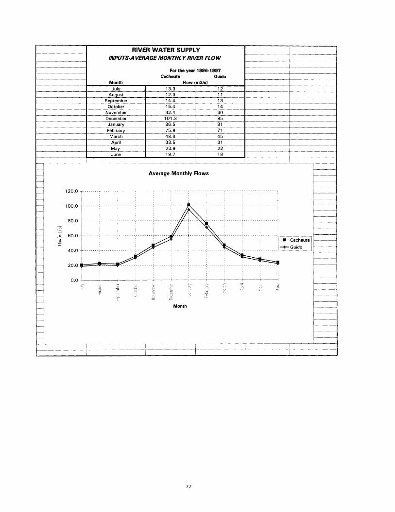
WATER DEMANDS (hm3)

Consumptive Demands Non-Consumptive Demands (Cachut & Computesl)

IRRIGATION Tract Demands Compuertae Potable Water Total INDUSTRIAL (YPFCTM,ORAS) Net Demand Beotrily

Month demnd/ha of heatares totalhm3) Superor Medo Inf'rior (S.5 m3/s) CTM(12m3/eI Consumed (6.5m3/s) (Compuertae) (Caoheuta)

July 8 74500 1 0 0 0 16.84 16.28 33.72 31.10 -16.84 14.26 26.76

~st 511 74500 38 19.30 6.40 12.37 16.84 16.28 71.19 31.10 -16.84 14.26 26.76

September 327 74500 24 12.35 4.09 7.92 16.84 16.28 57.48 31.10 -16.84 14.26 26.76

October 728 74500 54 27.50 9.11 17.63 16.84 16.28 87.36 31.10 16.84 14.26 26.76

November 1070 74500 80 40.42 13.39 25.91 16.84 16.28 112.84 31.10 -16.84 14.26 26.76

December 1249 74500 93 47.18 15.63 30.24 16.84 16.28 126.17 31.10 16.84 14.26 26.76

January 1205 74500 90 45.51 15.08 29.18 16.84 16.28 122.89 31.10 -16.84 14.26 28.76

February 842 74500 63 31.80 10.54 20.39 186.84 16.28 95.85 31.10 16.84 14.26 26.76

March 732 74500 55 27.65 9.16 17.72 16.84 16.28 87.65 31.10 -16.84 14.26 26.76

rl 409 74500 30 15.45 5.12 9.90 168.84 16.28 63.59 31.10 16.84 14.26 26.76

May 355 74500 26 13.41 4.44 8.60 16.84 16.28 59.57 31.10 -16.84 14.26 26.76

June 12 74500 1 0 0 0 16.84 16.28 34.01 31.10 16.84 14.26 26.76

Yearly Total 554.88 281.32 93.22 180.33 202.08 195.36 952.32 373.20 -202.08 171.12 321.12

Output Data for 1996-97 Flow ThroughStorage Flow in the Turbines for Spill

Flow Loss/Gain Demand Storage Electricity Release/Add. River Bed Elec. Gener. ReleaseMonth Nodes hm3/Mnth hm3/Mnth hm3/Mnth hm3 Mwh hm3/Mnth hm3/Mnth hm3/Mnth hm3/Mnth

July 1 -Guido 31.10 3.432-Cacheuta 34.53 0.00 420.00 18581.75 -15.49 5.00 45.02 0.003-Condarco 50.02 -1.77 9356.54 50.02 45.024-Compuertas 48.25 -2.23 16.845-Cipolletti 29.19 -1.68 34.016-Lujan 10.33 -0.30Groundwater 0.00

August 1-Guido 28.51 3.272-Cacheuta 31.78 0.00 404.51 38017.23 -67.44 5.00 94.23 0.003-Condarco 99.23 -1.77 19582.23 99.23 94.234-Compuertas 97.46 -2.23 16.845-Cipolletti 78.39 -0.70 90.226-Lujan 4.31 -19.03Groundwater 0.00 1

September 1-Guido 33.70 3.582-Cacheuta 37.28 0.00 337.06 28826.19 -41.39 5.00 73.66 0.003-Condarco 78.66 -1.77 15309.01 78.66 73.664-Compuertas 76.90 -2.23 16.845-Cipolletti 57.83 -0.70 69.666-Lujan 4.31 -12.18Groundwater 0.00

October 1-Guido 36.29 3.742-Cacheuta 40.02 0.00 295.68 30794.83 -45.68 5.00 80.70 0.003-Condarco 85.70 -1.77 16771.04 85.70 80.704-Compuertas 83.93 -2.23 16.845-Cipolletti 64.87 -0.70 114.476-Lujan 4.30 -27.12Groundwater 37.77

November 1-Guido 77.76 6.222-Cacheuta 83.98 0.00 250.00 29737.77 0.00 5.00 78.98 0.003-Condarco 83.98 -1.77 16414.68 83.98 78.984-Compuertas 82.22 -2.23 16.845-Cipolletti 63.15 -0.70 152.696-Lujan 4.30 -39.86Groundwater 77.70

December 1-Guido 246.24 16.332-Cacheuta 262.57 0.00 250.00 68122.12 80.88 5.00 176.70 0.003-Condarco 181.70 -1.77 36721.56 181.70 176.704-Compuertas 179.93 -2.23 16.845-Cipolletti 160.86 -0.70 172.706-Lujan 4.31 -46.53Groundwater 0.00

January 1-Guido 209.95 14.162-Cacheuta 224.11 0.00 330.88 68684.88 47.33 5.00 171.78 0.003-Condarco 176.78 -1.77 35699.70 176.78 171.784-Compuertas 175.01 -2.23 16.845-Cipolletti 155.95 -0.70 167.786-Lujan 4.31 -44.89

Groundwater 0.00February 1-G uido 184 .0 3 12 .60 3 8 2 6 .808_

2-Cacheuta 196.63 0.00 378.20 61401.10 41.80 5.00 149.84 0.003-Condarco 154.84 -1.77 31139.07 154.84 149.844-Compuertas 153.07 -2.23 16.845-Cipolletti 134.00 -3.31 127.216-Lujan 20.32 -31.36Groundwater 0.00

March 1-Guido 116.64 8.562-Cacheuta 125.20 0.00 420.00 49816.41 0.00 5.00 120.20 0.003-Condarco 125.20 -1.77 24979.57 125.20 120.204-Compuertas 123.43 -2.23 16.845-Cipolletti 104.36 -0.88 114.926-Lujan 5.40 -27.27Groundwater 0.00

April 1-Guido 80.35 6.382-Cacheuta 86.73 0.00 420.00 34318.26 -1.10 5.00 82.83 0.003-Condarco 87.83 -1.77 17213.38 87.83 82.834-Compuertas 86.06 -2.23 16.845-Cipolletti 66.99 -0.70 78.836-Lujan 4.31 -15.24Groundwater 0.00

May 1 -Guido 57.02 4.98

2-Cacheuta 62.00 0.00 418.90 31638.94 -19.79 5.00 76.79 0.003-Condarco 81.79 -1.77 15959.28 81.79 76.794-Compuertas 80.03 -2.23 16.84

5-Cipolletti 60.96 -0.70 72.796-Lujan 4.31 -13.22Groundwater 0.00

June 1 -Guido 46.66 4.362-Cacheuta 51.01 0.00 399.12 18454.68 0.99 5.00 45.02 0.003-Condarco 50.02 -1.77 9356.54 50.02 45.02

4-Compuertas 48.25 -2.23 16.845-Cipolletti 29.19 -1.62 34.466-Luian 9.95 -0.45Groundwater 0.00

Otput SummaryTotal Groundwater Pumped (hm3/yr) 115.47 Annual River Supply (hm3) 1235.86Electricity Generated at Cacheuta (Mwh) 478394.15 at CacheutalElectricity Generated at Condarco (Mwh) 248502.59Total Electricity Generated (Mwh) 726896.75Total Water Infiltration in Canal System (hm3/yr) -277.44Total Water Infiltration between Cach-Cippoll. -47.93

'Procedure which calculates water usage as a function of demands-Copyright Joseph Cavicchi 1996

'Declare Module variables

Dim FlowCach, FlowGuid, Demcons, Demnoncons, LossCachCon, LossConComDim DemCon, DemNCon, DemCip, StorCa, ElecCa, FlowCip, FlowLu, FlowGrwatDim LossCaCip, LossCipLu, LossCanals, LossComCip, StorReCa, SpillRe, DemConComDim StorAdd, StorSp, ElecFlowCa, ElecFlowCon, ReExc, LossCaCipMin, GainGuCaDim FlowCon, FlowCom, ElecCon, DemNConCom, DemNConCach, StorAddRe, FlowRivCa,FlowRivCon

'Declare constants

Const VolConv = 2.592Const StorMin = 250Const FlowLuMin = 5Const StorMax = 420Const ElecFlowMax = 207Const LF = 0.5Const AC = 1

'Procedures

Sub WaterUsageCalcsO

Static StorCanext(0 To 300) As VariantStorCanext(0) = StorMax

'Loops are begun to index model through both sheets and months

For J = 1 To 25 Step 1Sheets(J).Select

For I = 0 To 11 Step 1

'River water flows are taken from the input table to the water usage model

FlowGuid = Cells(43 + I, 12) * VolConv

'Determine the flows at Cacheuta/Condarco and the increase in flow between'Guido and Cacheuta

FlowCach = 1.559 + 1.06 * FlowGuidGainGuCa = FlowCach - FlowGuidFlowCon = FlowCach

'Operational decisions are made as a function of reservoir constraints

'Insert Storage value at beginning of period into model

StorCa = StorCanext(((J - 1) * 12) + I)StorSp = StorMax - StorCa

'Consumptive and non-consumptive demands are calculated or taken from demand table'Note: Non-Consumptive demand is used during June and July

DemNConCom = Cells(6 + I, 29)DemNConCach = Cells(6 + I, 30)DemNCon = DemNConCach + DemNConComDemConCom = Cells(6 + I, 24)LossCanals = Cells(6 + I, 21) * LF * -1 +

Cells(6 + I, 22) * LF * -1 +Cells(6 + I, 23) * LF * -1

DemCon = Cells(6 + I, 26) - LossCanals

'Determine the minimum losses that will occur between Cacheuta and Cipolletti'for usage in determining storage releases or additions

If DemCon > DemNCon And DemCon > ElecFlowMax ThenLossCaCipMinl = ((DemCon + FlowLuMin) A 0.58 * 1.086) * 1.1 * ACElseLossCaCipMinl = (FlowLuMin A 0.58) * 1.086 * AC + 1.24End If

'Check to see if demands are greater than electric station capacities

If DemCon + LossCaCipMinl / 1.1 + FlowLuMin > ElecFlowMax Then

LossCaCipMin = ((FlowLuMin + DemCon + (DemCon + LossCaCipMinl- ElecFlowMax)) A 0.58 * 1.086) * 1.05 * AC

ElseLossCaCipMin = LossCaCipMinl

End If

'Determine release from or addition to storage for the current period

'Examine situations where consumptive demand is greater than non-consumptive demand

'Determine if a release is required:

If DemCon > DemNCon And FlowCach < DemCon + FlowLuMin + LossCaCipMin _And StorCa - StorMin > DemCon + FlowLuMin + LossCaCipMin - FlowCachThenStorReCa = DemCon + FlowLuMin + LossCaCipMin - FlowCachStorAdd = 0

Elself DemCon > DemNCon And FlowCach < DemCon + FlowLuMin + LossCaCipMin _And StorCa - StorMin < DemCon + FlowLuMin + LossCaCipMin - FlowCachThenStorReCa = StorCa - StorMinStorAdd = 0

End If

'Determine if an addition should occur:

If DemCon > DemNCon And FlowCach > DemCon + FlowLuMin + LossCaCipMin AndFlowCach - DemCon - FlowLuMin - LossCaCipMin > StorSp _ThenStorAdd = StorSpStorReCa = 0

Elself DemCon > DemNCon And FlowCach > DemCon + FlowLuMin + LossCaCipMin AndFlowCach - DemCon - FlowLuMin - LossCaCipMin < StorSp_ThenStorAdd = FlowCach - DemCon - FlowLuMin - LossCaCipMinStorReCa = 0

End If

'Examine situations where non-consumptive demand is greater than consumptive demand

'Determine if a release is required:

If DemCon < DemNCon And FlowCach < DemNCon + FlowLuMin + LossCaCipMinAnd StorCa - StorMin > DemNCon + FlowLuMin + LossCaCipMin - FlowCach _ThenStorReCa = DemNCon + FlowLuMin + LossCaCipMin - FlowCachStorAdd = 0

Elself DemCon < DemNCon And FlowCach < DemNCon + FlowLuMin + LossCaCipMin _And StorCa - StorMin < DemNCon + FlowLuMin + LossCaCipMin - FlowCach _ThenStorReCa = StorCa - StorMinStorAdd = 0

End If

'Determine if an addition should occur:

If DemCon < DemNCon And FlowCach > DemNCon + FlowLuMin + LossCaCipMin And _FlowCach - DemNCon - FlowLuMin - LossCaCipMin > StorSp _ThenStorAdd = StorSpStorReCa = 0

Elself DemCon < DemNCon And FlowCach > DemNCon + FlowLuMin + LossCaCipMin AndFlowCach - DemNCon - FlowLuMin - LossCaCipMin < StorSp _ThenStorAdd = FlowCach - DemNCon - FlowLuMin - LossCaCipMinStorReCa = 0

'Caculate the quantity of water that is in storage at the end of the period

StorCanext(((J - 1) * 12) + I + 1) = StorCa - StorReCa + StorAdd

'Generate a release/addition value for the output table

If StorReCa = 0 ThenStorAddRe = StorAddElseStorAddRe = -StorReCaEnd If

'Determine the quantity of electricity generated at Cacheuta

If FlowCach - StorAdd + StorReCa - FlowLuMin > ElecFlowMax Then

ElecCa = ElecFlowMax * 0.87 * 2.73 *(174.5 - (StorMax - (StorCanext(((J - 1) * 12) + I + 1) + StorCa) / 2) * 0.094)

ElseElecCa = (FlowCach + StorReCa - StorAdd - FlowLuMin) * 0.87 * 2.73 *

(174.5 - (StorMax - (StorCanext(((J - 1) * 12)+ I + 1) + StorCa) / 2) * 0.094)

End If

'Determine the quantity of electricity generated at Condarco

If FlowCon - StorAdd + StorReCa - FlowLuMin > ElecFlowMax Then

ElecCon = ElecFlowMax * 0.87 * 2.73 * 87.5

ElseElecCon = (FlowCon + StorReCa - StorAdd - FlowLuMin) * 0.87 * 2.73 * 87.5

End If

'Determine what quantity of water was spilled during the current period

If FlowCach - StorAdd + StorReCa - FlowLuMin > ElecFlowMax AndStorCanext(((J - 1) * 12) + I + 1) = 420 ThenSpillRe = FlowCach - StorAdd + StorReCa - ElecFlowMax - FlowLuMin

ElseSpillRe = 0End If

End If

'Determine flow through the Cacheuta electricity station for the month

If FlowCach - StorAdd + StorReCa - FlowLuMin > ElecFlowMax ThenElecFlowCa = ElecFlowMax

ElseElecFlowCa = FlowCach + StorReCa - StorAdd - SpillRe - FlowLuMin

End If

'Determine flow through the Condarco electricity station for the month

If FlowCon - StorAdd + StorReCa - FlowLuMin > ElecFlowMax ThenElecFlowCon = ElecFlowMax

ElseElecFlowCon = FlowCon + StorReCa - StorAdd - SpillRe - FlowLuMin

End If

'Determine the flow that was in the river bed starting at dam gates during the period

If SpillRe = 0 ThenFlowRivCa = FlowCach + StorReCa - StorAdd - ElecFlowCa

ElseFlowRivCa = SpillRe + FlowLuMin

End If

LossCachCon = 0

'Determine the flow in the river at the outlet of the Condarco power station

FlowRivCon = FlowRivCa + LossCachCon + ElecFlowCon

'Calculate the losses between Condarco and Compuertas

LossConCom = (FlowRivCon - ElecFlowCon) ^ 0.58 * 1.086 * -1 * 0.64 * AC

'Determine the flow at Compuertas

FlowCom = FlowRivCon + LossConCom

'Calculate the flow at Cipolletti and the losses between Compuertas and Cipolletti

If FlowCom > ElecFlowCon + DemConCom + FlowLuMin ThenLossComCip = (FlowCom - ElecFlowCon) ^ 0.58 * 1.086 * -1 * 0.36 * ACFlowCip = FlowCom + LossComCip - DemConComElse

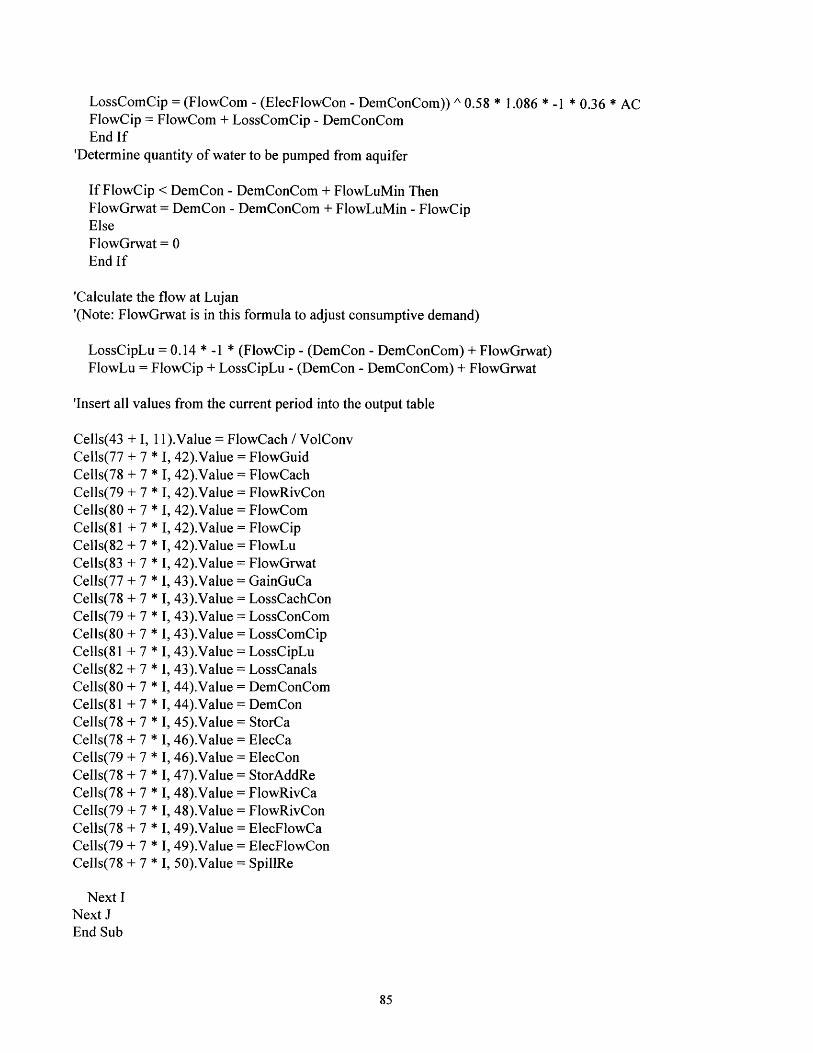
LossComCip = (FlowCom - (ElecFlowCon - DemConCom)) ^ 0.58 * 1.086 * -1 * 0.36 * ACFlowCip = FlowCom + LossComCip - DemConComEnd If

'Determine quantity of water to be pumped from aquifer

If FlowCip < DemCon - DemConCom + FlowLuMin ThenFlowGrwat = DemCon - DemConCom + FlowLuMin - FlowCipElseFlowGrwat = 0End If

'Calculate the flow at Lujan'(Note: FlowGrwat is in this formula to adjust consumptive demand)

LossCipLu = 0.14 * -1 * (FlowCip - (DemCon - DemConCom) + FlowGrwat)FlowLu = FlowCip + LossCipLu - (DemCon - DemConCom) + FlowGrwat

'Insert all values from the current period into the output table

Cells(43 + I, 11).Value = FlowCach / VolConvCells(77 + 7 * I, 42).Value = FlowGuidCells(78 + 7 * I, 42).Value = FlowCachCells(79 + 7 * I, 42).Value = FlowRivConCells(80 + 7 * I, 42).Value = FlowComCells(81 + 7 * I, 42).Value = FlowCipCells(82 + 7 * I, 42).Value = FlowLuCells(83 + 7 * I, 42).Value = FlowGrwatCells(77 + 7 * I, 43).Value = GainGuCaCells(78 + 7 * I, 43).Value = LossCachConCells(79 + 7 * I, 43).Value = LossConComCells(80 + 7 * I, 43).Value = LossComCipCells(81 + 7 * I, 43).Value = LossCipLuCells(82 + 7 * I, 43).Value = LossCanalsCells(80 + 7 * I, 44).Value = DemConComCells(81 + 7 * I, 44).Value = DemConCells(78 + 7 * I, 45).Value = StorCaCells(78 + 7 * I, 46).Value = ElecCaCells(79 + 7 * I, 46).Value = ElecConCells(78 + 7 * I, 47).Value = StorAddReCells(78 + 7 * I, 48).Value = FlowRivCaCells(79 + 7 * I, 48).Value = FlowRivConCells(78 + 7 * I, 49).Value = ElecFlowCaCells(79 + 7 * I, 49).Value = ElecFlowConCells(78 + 7 * I, 50).Value = SpillRe

Next INext JEnd Sub

Output Data for 1996-97 (No Damn) Flow ThroughStorage Flow in the Turbines for Spill

Flow Loss/Gain Demand Storage Electricity Release River Bed Elec. Gener. ReleaseMonth Nodes hm3/Mnth hm3/Mnth hm3/Mnth hm3 Mwh hm3/Mnth hm3/Mnth hm3/Mnth hm3/Mnth

July 1 -Guido 31.10 3.432-Cacheuta 34.53 0.00 0.00 1830.47 0.00 27.62 0.003-Condarco 34.53 -2.13 5593.11 27.624-Compuertas 32.40 -2.32 16.845-Cipolletti 13.23 -0.70 33.786-Lujan 4.30 -0.22

Groundwater 8.71August 1 -Guido 28.51 3.27

2-Cacheuta 31.78 0.00 0.00 1684.82 0.00 25.43 0.003-Condarco 31.78 -2.03 5148.06 25.434-Compuertas 29.75 -2.30 16.845-Cipolletti 10.61 -0.70 75.28

4.30 -14.05Groundwater 52.82

September 1 -Guido 33.70 3.582-Cacheuta 37.28 0.00 0.00 1976.12 0.00 29.82 0.003-Condarco 37.28 -2.23 6038.16 29.824-Compuertas 35.05 -2.35 16.845-Cipolletti 15.86 -0.70 60.106-Lujan 4.30 -8.99Groundwater 32.40

October 1 -Guido 36.29 3.74

2-Cacheuta 40.02 0.00 0.00 2121.78 0.00 32.02 0.03-Condarco 40.02 -2.32 6483.21 32.024-Compuertas 37.70 -2.38 16.84


November 1-Guido 77.76 6.222-Cacheuta 83.98 0.00 0.00 4452.21 0.00 67.19 0.003-Condarco 83.98 -3.57 13603.98 67.194-Compuertas 80.41 -2.81 16.84

5-Cipolletti 60.76 -0.70 121.406-Lujan 4.30 -29.43

Groundwater 48.79December 1-Guido 246.24 16.33

2-Cacheuta 262.57 0.00 0.00 6593.40 0.00 99.50 0.003-Condarco 262.57 -13.34 20146.49 99.504-Compuertas 249.23 -7.60 16.845-Cipolletti 224.79 -14.77 136.166-Lujan 90.71 -34.35

Groundwater 0.00January 1-Guido 209.95 14.16

2-Cacheuta 224.11 0.00 0.00 6593.40 0.00 99.50 0.003-Condarco 224.11 -11.41 20146.49 99.504-Compuertas 212.69 -6.58 16.84


February 1 -Guido 184.03 12.602-Cacheuta 196.63 0.00 0.00 6593.40 0.00 99.50 0.003-Condarco 196.63 -9.88 20146.49 99.504-Compuertas 186.75 -5.78 16.84


March 1-Guido 116.64 8.562-Cacheuta 125.20 0.00 0.00 6593.40 0.00 99.50 0.003-Condarco 125.20 -4.57 20146.49 99.504-Compuertas 120.63 -3.22 16.84

5-Cipolletti 100.57 -3.35 93.51S6-Lujan 20.55 -20.13 -

Groundwater 0.00 .3

April 1 -Guido 80.35 6.382-Cacheuta 86.73 0.00 0.00 4597.86 0.00 69.39 0.003-Condarco 86.73 -3.64 14049.03 69.39

4-Compuertas 83.10 -2.84 16.84


May 1-Guido 57.02 4.982-Cacheuta 62.00 0.00 0.00 3286.99 0.00 49.60 0.003-Condarco 62.00 -2.99 10043.59 49.60

4-Compuertas 59.01 -2.60 16.84

5-Cipolletti 39.57 -0.70 62.41

6-Lujan 4.30 -9.76Groundwater 11.00

June 1 -Guido 46.66 4.362-Cacheuta 51.01 0.00 0.00 2704.39 0.00 40.81 0.003-Condarco 51.01 -2.67 8263.40 40.81

4-Compuertas 48.34 -2.49 16.845-Cipolletti 29.01 -1.64 34.11

6-Lujan 10.10 -0.33Groundwater 0.00

on ut summar,Total Groundwater Pumped (hm3/yr) 216.58Electricity Generated at Cacheuta (Mwh) 49028.23Electricity Generated at Condarco (Mwh) 149808.48Total Electricity Generated (Mwh) 1 198836.72Total Water Infiltration in Canal System (hm3/yr) -204.82Total Water Infiltration between Cach-Cippoll. -104.08

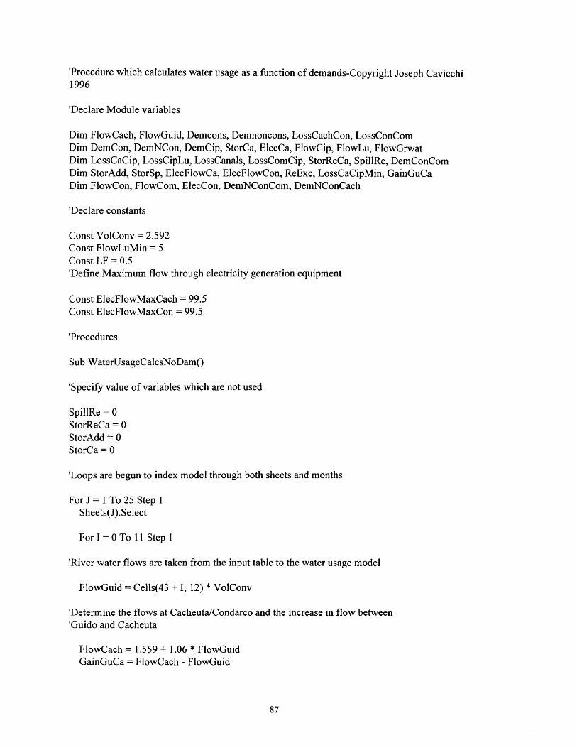
'Procedure which calculates water usage as a function of demands-Copyright Joseph Cavicchi1996

'Declare Module variables

Dim FlowCach, FlowGuid, Demcons, Demnoncons, LossCachCon, LossConComDim DemCon, DemNCon, DemCip, StorCa, ElecCa, FlowCip, FlowLu, FlowGrwatDim LossCaCip, LossCipLu, LossCanals, LossComCip, StorReCa, SpillRe, DemConComDim StorAdd, StorSp, ElecFlowCa, ElecFlowCon, ReExc, LossCaCipMin, GainGuCaDim FlowCon, FlowCom, ElecCon, DemNConCom, DemNConCach

'Declare constants

Const VolConv = 2.592Const FlowLuMin = 5Const LF = 0.5'Define Maximum flow through electricity generation equipment

Const ElecFlowMaxCach = 99.5Const ElecFlowMaxCon = 99.5

'Procedures

Sub WaterUsageCalcsNoDamO

'Specify value of variables which are not used

SpillRe = 0StorReCa = 0StorAdd = 0StorCa = 0

'Loops are begun to index model through both sheets and months

For J = 1 To 25 Step 1Sheets(J).Select

For I = 0 To 11 Step 1

'River water flows are taken from the input table to the water usage model

FlowGuid = Cells(43 + I, 12) * VolConv

'Determine the flows at Cacheuta/Condarco and the increase in flow between'Guido and Cacheuta

FlowCach = 1.559 + 1.06 * FlowGuidGainGuCa = FlowCach - FlowGuid

'Consumptive and non-consumptive demands are calculated or taken from demand table'Note: Non-Consumptive demand is used during June and July

DemNConCom = Cells(6 + I, 29)DemNCon = DemNConComDemConCom = Cells(6 + I, 24)LossCanals = Cells(6 + I, 21) * LF * -1 +

Cells(6 + I, 22) * LF * -1 +Cells(6 + I, 23) * LF * -1

DemCon = Cells(6 + I, 26) - LossCanals

'Examine the flow for the month to determine amount which can be used to generate electricity'I have decided that 80% can be used to generate electricity

'Determine the quantity of electricity generated at Cacheuta

If FlowCach > ElecFlowMaxCach * 1.2 Then

ElecCa = ElecFlowMaxCach * 0.87 * 2.73 * 27.9

ElseElecCa = (FlowCach * 0.87 * 2.73 * 27.9) * 0.8

End If'Determine flow through the Cacheuta electricity station for the month

If FlowCach > ElecFlowMaxCach ThenElecFlowCa = ElecFlowMaxCach

ElseElecFlowCa = FlowCach * 0.8

End If

'Calculate the losses between Cacheuta and Condarco

LossCachCon = 0

'Determine the flow at Condarco

FlowCon = FlowCach + LossCachCon

'Determine the quantity of electricity generated at Condarco

If FlowCon > ElecFlowMaxCon * 1.2 Then

ElecCon = ElecFlowMaxCon * 0.87 * 2.73 * 85.25

ElseElecCon = (FlowCon * 0.87 * 2.73 * 85.25) * 0.8

End If

'Determine flow through the Condarco electricity station for the month

If FlowCon > ElecFlowMaxCon ThenElecFlowCon = ElecFlowMaxCon

ElseElecFlowCon = FlowCon * 0.8

End If

'Calculate the losses between Condarco and Compuertas

LossConCom = (FlowCon - ElecFlowCon) ^ 0.58 * 1.086 * -1 * 0.64

'Determine the flow at Compuertas

FlowCom = FlowCon + LossConCom

'Calculate the flow at Cipolletti and the losses between Compuertas'and Cipolletti

LossComCip = (FlowCom - (ElecFlowCon - DemConCom)) ^ 0.58 * 1.086 * -1 * 0.36FlowCip = FlowCom + LossComCip - DemConCom

'Determine quantity of water to be pumped from aquifer

If FlowCip < DemCon - DemConCom + FlowLuMin ThenFlowGrwat = DemCon - DemConCom + FlowLuMin - FlowCipElseFlowGrwat = 0End If

'Calculate the flow at Lujan'(Note: FlowGrwat is in this formula to adjust consumptive demand)

LossCipLu = 0.14 * -1 * (FlowCip - (DemCon - DemConCom) + FlowGrwat)FlowLu = FlowCip + LossCipLu - (DemCon - DemConCom) + FlowGrwat

'Insert all values from the current period into the output table

Cells(43 + I, 11).Value = FlowCach / VolConvCells(77 + 7 * I, 42).Value = FlowGuidCells(78 + 7 * I, 42).Value = FlowCachCells(79 + 7 * I, 42).Value = FlowConCells(80 + 7 * I, 42).Value = FlowComCells(78 + 7 * I, 44).Value = EmptyCells(81 + 7 * I, 42).Value = FlowCip

Cells(82 + 7 * I, 42).Value = FlowLuCells(83 + 7 * I, 42).Value = FlowGrwatCells(77 + 7 * I, 43).Value = GainGuCaCells(78 + 7 * I, 43).Value = LossCachConCells(79 + 7 * I, 43).Value = LossConComCells(80 + 7 * I, 43).Value = LossComCipCells(81 + 7 * I, 43).Value = LossCipLuCells(82 + 7 * I, 43).Value = LossCanalsCells(80 + 7 * I, 44).Value = DemConComCells(81 + 7 * I, 44).Value = DemConCells(78 + 7 * I, 45).Value = StorCaCells(78 + 7 * I, 46).Value = ElecCaCells(79 + 7 * I, 46).Value = ElecConCells(78 + 7 * I, 47).Value = StorReCaCells(78 + 7 * I, 49).Value = ElecFlowCaCells(79 + 7 * I, 49).Value = ElecFlowConCells(78 + 7 * I, 50).Value = SpillRe

Next INext JEnd Sub

Declare Variablesand Constants

Set Initial Storage

ogin Loops

J = 1 to 25 Years

= 1 to 12 Months

Obtain FlowGuid fromRiver Flow Table

Calculate FlowCach

Input Initial Storage

Evalaute Demand

Calculate Minimum LossesBetween Cach & Cip

Determine Whether Release orAddition to Storage is Required

Calculate Storage at theEnd of the Period I

Calculate theAmount of Electricity

Generated at Cach.

Calculate the SpillRelease for the Period

4I I

I I

I I

I I

I II I

I I

I I

Determine the FlowGenerating Electricityat Con. During Period

Determine the Flowin the River Bed

Calculate the Lossesand Flows Between

Con. and Cip.

Calculate the Amount ofGroundwater Required

Calculate theAmount of Electricity

Generated at Con.

Determine the FlowGenerating Electricityat Cach. During Period

y

r

b;-, ---

i ; r

r

-A

I

Flow Chart - Model with Dam

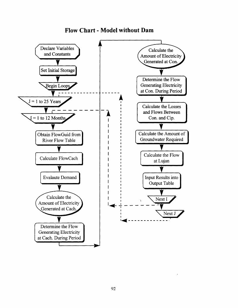
Obtain FlowGuid fromRiver Flow Table

/ Calculate the ,Amount of Electricity,Generated at Con. ,

Determine the FlowGenerating Electricityat Con. During Period

Calculate the Lossesand Flows Between

Con. and Cip.

Calculate the Amount ofGroundwater Required

'14--- -. -------------Determine the Flow

Generating Electricityat Cach. During Period

1

Irt

Flow Chart - Model without Dam

Investment ($000) 1 Benefits (8000)Dam Projects Interest during Construction 10%

Discount rate 12% Benefit Factor 1 1Elec.Value($/Mwh) 30

Potrerillos (state) Potrerillos (Inves.) Total Electricity Tourism Floods Agriculture(net)

-69,695 -6,969 0 -6,969 0 0 0

-32,952 -10,265 0 -10,265 0 0 0

-87,191 -18,984 0 -18,984 0 0 0

-72,903 -26,274 0 -26,274 0 0 0-28,869 -29,161 0 -29,161 11,364 0 0

-48,866 -1,441 -50,307 15,842 7,983 1,000 412

-48,866 -1,441 -50,307 10,522 7,983 1,000 1,036-48,866 -1,441 -50,307 11,514 7,983 1,000 1,888-48,866 -1,441 -50,307 17,745 7,983 1,000 2,200

-48,866 -1,441 -50,307 17,032 7,983 1,000 874-48,866 -1,441 -50,307 16,055 7,983 1,000 903-48,866 -1,441 -50,307 15,088 7,983 1,000 768

-48,866 -1,441 -50,307 9,398 7,983 1,000 2,040

-48,866 -1,441 -50,307 17,558 7,983 1,000 2,088-48,866 -1,441 -50,307 20,699 7,983 1,000 1,595-48,866 -1,441 -50,307 20,915 4,160 1,000 1,960-48,866 -1,441 -50,307 21,658 4,160 1,000 2,303

-48,866 -1,441 -50,307 16,376 4,160 1,000 1,943

-48,866 -1,441 -50,307 23,714 4,160 1,000 2,836-48,866 -1,441 -50,307 24,038 4,160 1,000 2,634

-48,866 -1,441 -50,307 22,132 4,160 1,000 2,510-48,866 -1,441 -50,307 20,501 4,160 1,000 1,948

-48,866 -1,441 -50,307 22,725 4,160 1,000 2,622-48,866 -1,441 -50,307 25,974 4,160 1,000 2,888

-48,866 -1,441 -50,307 20,039 4,160 1,000 1,729

-48,866 -1,441 -50,307 19,114 0 1,000 3,213

-48,866 -1,441 -50,307 15,291 0 1,000 4,550

-48,866 -1,441 -50,307 21,451 0 1,000 4,894

-48,866 -1,441 -50,307 20,449 0 1,000 3,657

-48,866 -1,441 -50,307 19,291 0 1,000 3,316

($238,862.17) ($279,047.04) ($11,301.96) ($317,164.54) $91 098.49 $33,475.08 $4,984.46 $13,007.56

93

S 831 T-1.1as5

162

3

PI

460 -724

T [

444556

-740-633

.n~n-220-222

637966

-548218

,,.o

I

800.00

700.00

600.00

500.00

E

EE400.00

300.00

7w--

I -I ICC) C) ~ - i ') 1 L :lriij ,z i~ ,7 < c . c i• ,;• <• ,• 1 i:: l-

Year

----------:--l

I --l-l_--------l-- Cl

200.00 1

100.00

0.00

--------1

---- --------- -------;----i----:---

--- With Reservoir

--- tWithout Reservoir

-----------. . .--- _ _- -- --------

--------

j

Groundwater Pumped with and without Reservoir

I I I 1 7-t u, rr,

I·, t u

i,1 ~-1 ~I -1 ~.I I'

Electricity Generated with and without Dam

--- Electricity Generated Without Dam

1200 -- Electricity Generated with Dam

1000

800

600

400

200

0

( k( -I I- -, [ ,

I I j

Year

97

m

~ ------ · ·

-------- -- ----- ---- ----- ---- -----------

--- ---- ----7 1 .... ... ........... 2 ------------------- ---------- ....... ....

----- -- --- ---- ---- ----------------------------------- ----------------------- -----------

----------- -- ---- -- ---- -------

------------- --------- ------I ------- ---- ------------ ------- ----- ----- ------------- - ---

, -) --

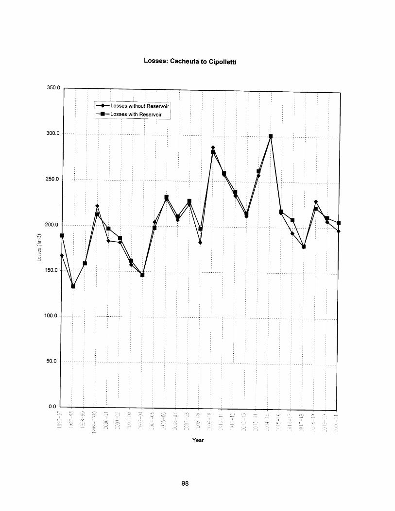
Losses: Cacheuta to Cipolletti

C- x I

Year

98

300.C

250.C

200.0

150.0

100.0

50.0

i I i C

r

Year

800000.00

700000.00

600000.00

500000.00

400000.00

300000.00

200000.00

100000.00

0.00

Electricity Generation Comparison

'1, C (-: D l CD CI) I i,--

Results

100

1

lm

101

FUTURE #1Scenario Water Demand Variations Water Loss Variations

Potable (OSM) Industrial Irrigation Canal Marginal Canal Lining Aguas Claras Improved Total Quan. of(Clear Water) Usage GW Pmpd(hm3)

Existing Cach/Con Arrangement 6/95 Forecast Constant 74,500 hectares No No No No 4682.110.) Potrerillos 6/95 Forecast Constant 74,500 hectares No No No No 2419.81.) Potrerillos w/ 500hm3 Util. 6/95 Forecast Constant 74,500 hectares No No No No 1575.672.) Potrenlos w/clear water (15%) 6/95 Forecast Constant 74,500 hectares No Yes Yes (15%) No 2658.43.) Potrerillos w/clear water (30%) 6/95 Forecast Constant 74,500 hectares No Yes Yes (30%) No 2922.644.) Potrerillos w/ Marginal Canal 6/95 Forecast Constant 74,500 hectares Yes No No No 1443.395.) Marginal Canal 6/95 Forecast Constant 74,500 hectares Yes No No No 3777.686.) Marginal Canal with Enlarged 6/95 Forecast Constant 74,500 hectares Yes No No No 3774.8Condarco7.) Marginal Canal plus 12% 6/95 Forecast Constant 74,500 hectares Yes Yes (12%) No No 3442.55Reduction in Canal Losses8.) Marginal Canal plus 24% 6/95 Forecast Constant 74,500 hectares Yes Yes (24%) No No 3088.23Reduction in Canal Losses9.) 24% Loss Reduction in Canals 6/95 Forecast Constant 74,500 hectares No Yes (24%) No No 3903.610.) 12% Loss Reduction in Canals 6/95 Forecast Constant 74,500 hectares No Yes (12%) No No 4308.511.) Existing w 112% + 10% Loss 6/95 Forecast Constant 74,500 hectares No Yes (12%) No Yes (10%) 3989Reduction vs. existing Cach/Con12.) Existing w/MC+ 12% + 10% 6/95 Forecast Constant 74,500 hectares Yes Yes (12%) No Yes (10%) 3162.25Loss Reduction vs. ExistingCach/Con

Scenario Pertinent Results Compiled From MultipleiModel Run*s .Total Infiltration (hm3) Ave.quan.of G Ave. quan. of NPV NPV Total Cost IRR

Farms/Canals Cach-Cip pumped (hm3/y Elec. (Gwh/yr) Investor State Finan. NPV ($000) State Finan.Existing Cach/Con Arrangement 6935.95 5170.8 187.28 245.84 N.A. N.A. N.A. N.A.0.) Potrerillos 6935.95 5251.17 96.79 876.17 (173,622) (93,190) 238,862 7%1.) Potrerillos w/ 500hm3 Util. 6935.95 5273.81 63.03 938.8 (365,703) (236,722) 360,356 4%2.) Potrerillos w/clear water (15%) 6935.95 6023.13 106.34 877.56 (178,154) (97,872) 241,559 7%3.) Potrerillos w/clear water (30%) 6935.95 6789.8 116.9 879.5 (182,330) (102,167) 244,919 7%4.) Potrerillos w/ Marginal Canal 6935.95 1774.58 57.74 866 (182,891) (102,853) 247,711 6%5.) Marginal Canal 6935.95 3142.72 151.11 245.84 (14,360) (12,519) 24,370 2%6.) Marginal Canal with Enlarged 6935.95 2531.68 150.99 304.52 (40,594) (35,908) 62,227 2%Condarco7.) Marginal Canal plus 12% 6159.12 3142.72 137.7 245.84 (13,087) (11,057) 27,067 4%Reduction in Canal Losses8.) Marginal Canal plus 24% 5278.26 3142.72 123.53 245.84 (12,370) (10,086) 30,427 6%Reduction in Canal Losses9.) 24% Loss Reduction in Canals 5278.26 5170.75 156.14 245.84 (11,473) (9,857) 21,578 3%10.) 12% Loss Reduction in Canals 6159.1 5170.75 172.34 245.84 (13,451) (12,089) 18,21811.) Existing w /12% + 10% Loss 5465.5 5170.75 159.57 245.84 (83,923) (76,656) 96,393Reduction vs. existing Cach/Con12.) Existing w/MC+ 12% + 10% 5465.5 3142.72 126.49 245.84 (85,658) (77,723) 105,242Loss Reduction vs. ExistingCach/Con

i

FUTURE #2Scenario Water Demand Variations Water Loss Varlations


Existing Cach/Con Arrangement 6/95 Forecast Constant 55,000 hectares No No No No 23830.) Potrerillos 6/95 Forecast Constant 55,000 hectares No No No No 873.891.) Potrerillos w/ 500hm3 Util. 6/95 Forecast Constant 55,000 hectares No No No No 258.722.) Potrerillos w/clear water (15%) 6/95 Forecast Constant 55,000 hectares No Yes Yes (15%) No 977.693.) Potrerillos w/clear water (30%) 6/95 Forecast Constant 55,000 hectares No Yes Yes (30%) No 1087.34.) Potrerillos w/ Marginal Canal 6/95 Forecast Constant 55,000 hectares Yes No No No 388.465.) Marginal Canal 6/95 Forecast Constant 55,000 hectares Yes No No No 1781.046.) Marginal Canal with Enlarged 6/95 Forecast Constant 55,000 hectares Yes No No No 1796.78Condarco7.) Marginal Canal plus 12% 6/95 Forecast Constant 55,000 hectares Yes Yes (12%) No No 1614.68Reduction in Canal Losses8.) Marginal Canal plus 24% 6/95 Forecast Constant 55,000 hectares Yes Yes (24%) No No 1436.35Reduction in Canal Losses9.) 24% Loss Reduction in Canals 6/95 Forecast Constant 55,000 hectares No Yes (24%) No No 1973.910.) 12% Loss Reduction in Canals 6/95 Forecast Constant 55,000 hectares No Yes (12%) No No 2187.0711.) Existing w /12% + 10% Loss 6/95 Forecast Constant 55,000 hectares No Yes (12%) No Yes (10%) 2018.62Reduction vs. existing Cach/Con12.) Existing w/MC+ 12% + 10% 6/95 Forecast Constant 55,000 hectares Yes Yes (12%) No Yes (10%) 1473.16Loss Reduction vs. ExistingCach/Con

Scenario Pertinent Results Compiled From Multiple Model RunsTotal Infiltration (hm3) Ave.quan.of G Ave. quan. of NPV NPV Total Cost IRR

Farms/Canals Cach-Cip pumped (hm3/y Elec. (Gwhlyr) Investor State Finan. NPV ($000) State Finan.Existing Cach/Con Arrangement 5120.5 5170.8 95.32 245.84 N.A. N.A. N.A. N.A.0.) Potrerillos 5120.5 5227.5 34.96 860.10 (176,987) (96,554) 238,862 7%1.) Potrerillos w/ 500hm3 Util. 5120.5 5249.5 10.35 925.25 (368,901) (239,920) 360,356 3%2.) Potrerillos w/clear water (15%) 5120.5 5994 39.11 861.4 (180,071) (99,759) 241,559 7%3.) Potrerillos w/clear water (30%) 5120.5 6758.6 43.49 863.11 (183,628) (103,466) 244,919 6%4.) Potrerillos w/ Marginal Canal 5120.5 1841 15.54 857.82 (186,812) (106,774) 247,711 6%5.) Marginal Canal 5120.5 3142.72 71.24 245.84 (16,868) (15,027) 24,370 n/a6.) Marginal Canal with Enlarged 5120.5 2531.68 71.87 304.52 (45,924) (41,034) 62,227 0%Condarco7.) Marginal Canal plus 12% 4547 3142.72 64.59 245.84 (17,249) (15,218) 27,067 0%Reduction in Canal Losses8.) Marginal Canal plus 24% 3896.7 3142.72 57.45 245.84 (18,266) (15,982) 30,427 0%Reduction in Canal Losses9.) 24% Loss Reduction in Canals 3896.7 5170.8 78.96 245.84 (15,957) (14,342) 21,578 n/a10.) 12% Loss Reduction in Canals 4547 5170.8 87.48 245.84 (15,183) (13,821) 18,218 n/a11.) Existing w 1/12% + 10% Loss 4034.95 5170.8 80.74 245.84 (88,929) (81,663) 96,393 n/aReduction vs. existing Cach/Con12.) Existing w/MC+ 12% + 10% 4034.95 3142.72 58.93 245.84 (91,180) (83,245) 105,242 n/aLoss Reduction vs. ExistingCach/Con

Scenar•o Water D•eqnhnd Variations __Wa _______ Loss Variations _________ ______.._


Existing Cach/Con Arrangement 6/95 Forecast Constant 65,000 hectares No No No No 3454.230.) Potrerillos 6/95 Forecast Constant 65,000 hectares No No No No 1464.51.) Potrerillos w/ 500hm3 Util. 6/95 Forecast Constant 65,000 hectares No No No No 821.882.) Potrerillos w/clear water (15%) 6/95 Forecast Constant 65,000 hectares No Yes Yes (15%) No 16373.) Potrerillos w/clear water (30%) 6/95 Forecast Constant 65,000 hectares No Yes Yes (30%) No 1843.14.) Potrerillos w/ Marginal Canal 6/95 Forecast Constant 65,000 hectares Yes No No No 913.385.) Marginal Canal 6/95 Forecast Constant 65,000 hectares Yes No No No 2711.86.) Marginal Canal with Enlarged 6/95 Forecast Constant 65,000 hectares Yes No No No 2725.4Condarco7.) Marginal Canal plus 12% 6/95 Forecast Constant 65,000 hectares Yes Yes (12%) No No 2466.47Reduction in Canal Losses8.) Marginal Canal plus 24% 6/95 Forecast Constant 65,000 hectares Yes Yes (24%) No No 2204.23Reduction in Canal Losses9.) 24% Loss Reduction in Canals 6/95 Forecast Constant 65,000 hectares No Yes (24%) No No 2869.410.) 12% Loss Reduction in Canals 6/95 Forecast Constant 65,000 hectares No Yes (12%) No No 3167.811.) Existing w /12% + 10% Loss 6/95 Forecast Constant 65,000 hectares No Yes (12%) No Yes (10%) 2931.79Reduction vs. existing Cach/Con12.) Existing w/MC+ 12% + 10% 6/95 Forecast Constant 65,000 hectares Yes Yes (12%) No Yes (10%) 2258.83Loss Reduction vs. ExistingCach/Con

Scenario Pertinent Results Compiled From MultlpeModel RunsTotal Infiltration (hm3) Ave.quan.of G Ave. quan. of NPV NPV Total Cost IRR

Farms/Canals Cach-CIp pumped (hm3/y Elec. (Gwhlyr) Investor State Finan. NPV ($000) State Finan.Existing Cach/Con Arrangement 6051.5 5170.8 138.17 245.84 N.A. N.A. N.A. N.A.0.) Potredllos 6051.5 5239.52 58.58 867.81 (174,399) (93,966) 238,862 7%1.) Potrerillos w/ 500hm3 Util. 6051.5 5261.31 32.88 932.91 (383,665) (254,684) 360,356 3%2.) Potrerillos w/clear water (15%) 6051.5 6010.5 65.48 870 (177,965) (97,653) 241,559 7%3.) Potrerillos w/clear water (30%) 6051.5 6777.34 73.72 871.88 (182,208) (102,045) 244,919 7%4.) Potrerillos w/ Marginal Canal 6051.5 1818.44 36.54 859.55 (186,812) (106,774) 247,711 6%5.) Marginal Canal 6051.5 3142.72 108.47 245.84 (15,728) (13,887) 24,370 0%6.) Marginal Canal with Enlarged 6051.5 2531.68 109.02 304.52 (42,111) (37,425) 62,227 1%Condarco7.) Marginal Canal plus 12% 5373.7 3142.72 98.66 245.84 (15,335) (13,304) 27,067 2%Reduction in Canal Losses8.) Marginal Canal plus 24% 4605.2 3142.72 88.17 245.84 (15,529) (13,245) 30,427 3%Reduction in Canal Losses9.) 24% Loss Reduction in Canals 4605.2 5170.8 114.8 245.84 (14,228) (12,612) 21,57810.) 12% Loss Reduction in Canals 5373.7 5170.8 126.71 245.84 (14,305) (12,943) 18,21811.) Existing w /12% + 10% Loss 4768.58 5170.8 117.27 245.84 (87,381) (80,114) 96,393Reduction vs. existing Cach/Con12.) Existing w/MC+ 12% + 10% 4768.58 3142.72 90.35 245.84 (88,619) (80,684) 105,242Loss Reduction vs. ExistingCach/Con

II

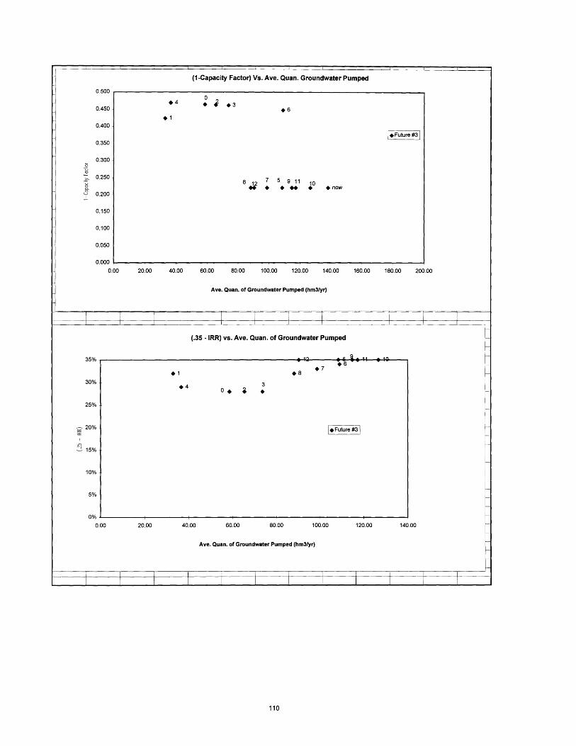
0.00 20.00 40.00 60.00 80.00 100.00 120.00 140.00 160.00 180.00 200.00


I I I I

(.35 - IRR) vs. Ave. Quan. of Groundwater Pumped

Ca 44

0.00 20.00 40.00 60.00 80.00


I I- I-- I I Iri-Tti-~

0.500

0.450

0.400

0.350 -

0.300

0.250

0.200

0.150 -

0.100 -

0.050

0.000

30%

25%

20%

15%

10%

5%

-68 7

30o

F Future #3

100.00 120.00 140.00

/ I I I II I - - 7 -

I 1I - ! - I1 t1 - -

- · · · · ·

i

(1-Capacity Factor) Vs. Ave. Quan. Groundwater Pumped

0e4 * *3

*6e1

F*Future #3]

7 5 9 11 10S* * * now

I I I I I I I I I I

+

L

Present Value Costs Vs. Average Quantity of Ground Water Pumped

400,000

350,000

300,000

250,000

200,000

150,000-

100,000 -

50,000 -

0

0.00 20.00 40.00 60.00 80.00 100.00

Ave. Quantity of Ground Water Pumped (hm3lyr)

i

*Future#3

*4 *0 *2 *3

*12

S6

*8 *9 #5 #9 10

120.00 140.00

Present Value Costs vs. Ratio of GW Pumped and Infiltration Between Cach-Cip'fuu~uu

10u,uuu

350,000

300,000-

~250,000

200,000-

150,000o

100,000

50,000 -

0

0.00 0.20 0.40 0.60 0.80 1.00 1.20

Ground Water Pumpedllnfiltration Cach-Cip

01

3

2%

* 1211

7 59 10 *8

i

I

---~-----~---~----~----~----~--

/ I I I I I

' ; : FUTU I E4Scenar~io WaterDemand Variations WaterLoss Vari ions _


Existing Cach/Con Arrangement 6/95 Forecast Constant 85,000 hectares No No No No 6267.30.) Potrerillos 6/95 Forecast Constant 85,000 hectares No No No No 3780.11 .) Potrerillos w/ 500hm3 Util. 6/95 Forecast Constant 85,000 hectares No No No No 2577.82.) Potrerillos w/clear water (15%) 6/95 Forecast Constant 85,000 hectares No Yes Yes (15%) No 4103.983.) Potrerillos w/clear water (30%) 6/95 Forecast Constant 85,000 hectares No Yes Yes (30%) No 4431.234.) Potrerillos w/ Marginal Canal 6/95 Forecast Constant 85,000 hectares Yes No No No 2405.745.) Marginal Canal 6/95 Forecast Constant 85,000 hectares Yes No No No 5204.266.) Marginal Canal with Enlarged 6/95 Forecast Constant 85,000 hectares Yes No No No 5155.66Condarco7.) Marginal Canal plus 12% 6/95 Forecast Constant 85,000 hectares Yes Yes (12%) No No 4750.7Reduction in Canal Losses8.) Marginal Canal plus 24% 6/95 Forecast Constant 85,000 hectares Yes Yes (24%) No No 4254.45Reduction in Canal Losses9.) 24% Loss Reduction in Canals 6/95 Forecast Constant 85,000 hectares No Yes (24%) No No 5219.9110.) 12% Loss Reduction in Canals 6/95 Forecast Constant 85,000 hectares No Yes (12%) No No 5767.9211.) Existing w /12% + 10% Loss 6/95 Forecast Constant 85,000 hectares No Yes (12%) No Yes (10%) 5346.33Reduction vs. existing Cach/Con12.) Existing w/MC+ 12% + 10% 6/95 Forecast Constant 85,000 hectares Yes Yes (12%) No Yes (10%) 4358,25Loss Reduction vs. ExistingCach/Con

Scenario PertUnent Resuts Compiled From Multiple Model RunsTotal Infiltration (hm3) Ave.quan.of GW Ave. quan. of NPV NPV Total Cost IRR

FarmslCanals Cach-CIp pumped (hm3ly Elec. (Gwhlyr) Investor State Finan. NPV ($000) State Finan.Existing Cach/Con Arrangement 7913.5 5170.75 250.70 245.84 N.A. N.A. N.A. N.A.0.) Potrerillos 7913.5 5257.47 151.21 882.15 (173,229) (92,797) 238,862 7%1.) Potrerillos w/ 500hm3 Util. 7913.5 5286.24 103.11 940.53 (364,187) (235,206) 360,356 4%2.) Potrerillos w/clear water (15%) 7913.5 6016.62 164.16 881.9 (177,988) (97,676) 241,559 7%3.) Potrerillos w/clear water (30%) 7913.5 6788.16 177.25 881.47 (183,193) (103,031) 244,919 7%4.) Potrerillos w/ Marginal Canal 7913.5 1720.36 96.23 874.33 (167,038) (87,000) 247,711 8%5.) Marginal Canal 7913.5 3142.72 208.17 245.84 (13,191) (11,350) 24,370 3%6.) Marginal Canal with Enlarged 7913.5 2531.68 206.23 304.52 (39,274) (34,574) 62,227 2%Condarco7.) Marginal Canal plus 12% 7027.19 3142.72 190.03 245.84 (11,034) (8,990) 27,067 6%Reduction in Canal Losses8.) Marginal Canal plus 24% 6022.17 3142.72 170.18 245.84 (9,028) (6,730) 30,427 8%Reduction in Canal Losses9.) 24% Loss Reduction in Canals 6022.17 5170.75 208.8 245.84 (9,993) (8,377) 21,578 5%10.) 12% Loss Reduction in Canals 7027.19 5170.75 230.72 245.84 (12,387) (11,025) 18,218 n/a11.) Existing w /12% + 10% Loss 6235.84 5170.75 213.85 245.84 (83,635) (76,368) 96,393 n/aReduction vs. existing Cach/Con12.) Existing wlMC+ 12% + 10% 6235.84 3142.72 174.33 245.84 (82,586) (74,636) 105,242 n/aLoss Reduction vs. ExistingCach/Con

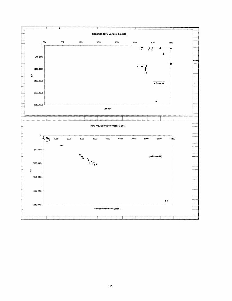
Scenario NPV versus .35-IRR

10% 15% 20% 25% 30% 35%0%0

(50,000)

(100,000)

(150,000)

(200,000)

(250,000)

Scenario Water cost ($1hm3)

.35-IRR

8 7 9

3

*FUtr #

19 1000 2000 3000 4000 5000 6000 7000 8000 9000 101

12

0 2

•1

NPV vs. Scenario Water Cost

0

(50,000)

(100,000)

(150,000)

(200,000)

(~50n non

00

S I J 1 i i I i I i I 1 i

---~-~--~---~'~-~--~----~---7----~-----~

!00

V

---

Potable (OSM) Industrial Irrigation Canal Marginal Canal ining Aguas Claras Improved Total Quan. of(Clear Water) Usage GW Pmpd(hm3)

Existing Cach/Con Arrangement % Yearly Growt Constant 74,500 hectares No No No No 5164.640.) Potrerillos % Yearly Growt Constant 74,500 hectares No No No No 2780.461.) Potrerillos w/ 500hm3 Util. % Yearly Growt Constant 74,500 hectares No No No No 1854.012.) Potrerillos w/clear water (15%) % Yearly Growt Constant 74,500 hectares No Yes Yes (15%) No 3061.63.) Potrerillos w/clear water (30%) % Yearly Growt Constant 74,500 hectares No Yes Yes (30%) No 3362.834.) Potrerillos w/ Marginal Canal % Yearly Growt Constant 74,500 hectares Yes No No No 1665.515.) Marginal Canal % Yearly Growt Constant 74,500 hectares Yes No No No 4201.76.) Marginal Canal with Enlarged % Yearly Growt Constant 74,500 hectares Yes No No No 4199.04Condarco7.) Marginal Canal plus 12% % Yearly Growt Constant 74,500 hectares Yes Yes (12%) No No 3849.9Reduction in Canal Losses8.) Marginal Canal plus 24% % Yearly Growt Constant 74,500 hectares Yes Yes (24%) No No 3464.25Reduction in Canal Losses9.) 24% Loss Reduction in Canals % Yeady Growt Constant 74,500 hectares No Yes (24%) No No 4346.2510.) 12% Loss Reduction in Canals % Yearly Growt Constant 74,500 hectares No Yes (12%) No No 4765.9311.) Existing w 1/12% + 10% Loss % Yearly Growt Constant 74,500 hectares No Yes (12%) No Yes (10%) 4433.62Reduction vs. existing Cach/Con12.) Existing w/MC+ 12% + 10% % Yearly Growt Constant 74,500 hectares Yes Yes (12%) No Yes (10%) 3543.95Loss Reduction vs. ExistingCach/Con

Total Infiltration (hm3) Ave.quan.of G Ave. quan. of NPV NPV Total Cost IRRFarms/Canals Cach-CIp pumped (hm3ly Elec. (Gwhlyr) Investor State Flnan. NPV ($000) State Finan.

Existing Cach/Con Arrangement 6935.95 5170.8 206.59 245.84 N.A. N.A. N.A. N.A.0.) Potrerillos 6935.95 5266.26 111.22 877.99 (172,890) (92,458) 238,862 7%1.) Potrerillos w/ 500hm3 Util. 6935.95 5289.79 74.16 940.4 (364,644) (235,663) 360,356 4%2.) Potrerillos w/clear water (15%) 6935.95 6038.07 122.46 880.14 (178,987) (98,795) 241,559 7%3.) Potrerillos w/clear water (30%) 6935.95 6805.3 134.51 882.09 (186,066) (106,174) 244,919 6%4.) Potrerillos w/ Marginal Canal 6935.95 1782.83 66.62 867.64 (162,116) (81,684) 247,711 8%5.) Marginal Canal 6935.95 3204.03 168.07 245.84 (13,774) (11,933) 24,370 2%6.) Marginal Canal with Enlarged 6935.95 2593.9 167.96 304.52 (40,194) (35,494) 62,227 2%Condarco7.) Marginal Canal plus 12% 6159.1 3204.03 154 245.84 (15,156) (12,908) 27,067 4%Reduction in Canal Losses8.) Marginal Canal plus 24% 5278.26 3204.03 138.57 245.84 (17,446) (14,690) 30,427 4%Reduction in Canal Losses9.) 24% Loss Reduction in Canals 5278.26 5170.8 173.85 245.84 (17,980) (15,893) 21,578 0%10.) 12% Loss Reduction in Canals 6159.1 5170.8 190.64 245.84 (16,011) (14,431) 18,21811.) Existing w 1/12% + 10% Loss 5465.53 5170.8 177.34 245.84 (88,125) (80,640) 96,393Reduction vs. existing Cach/Con12.) Existing w/MC+ 12% + 10% 5465.53 3204.03 141.76 245.84 (87,525) (79,371) 105,242Loss Reduction vs. ExistingCach/Con

A Multi-Attribute Tradeoff Analysis for Water Resource ...

Documents

Transcript of A Multi-Attribute Tradeoff Analysis for Water Resource ...