A Mathematical Model of Biofilm Growth onDegradable Substratum

Jack M. Hughes*

Sponsor: Hermann J. Eberl�

Department of Mathematics and Statistics, University of Guelph

Guelph, Ontario, Canada N1G2W1

April 12, 2020

Abstract

We derive a mathematical model for biofilm growth on a degradable substra-tum. The starting point is the one-dimensional Wanner-Gujer biofilm model. Theprocesses included are diffusion of a dissolved growth controlling substrate into thebiofilm, cell lysis, detachment of biomass, and growth from substrate conversionand substratum degradation. The resulting model is a system of two non-linearordinary differential equations, the evaluation of the right-hand side of which re-quires the solution of a semi-linear two-point boundary value problem. We performstandard analysis from the existence and uniqueness of solutions to equilibriumand stability analysis. Finally, we study our model through numerical simulationsand investigate how biofilms evolve on degradable substratum. We find in our set-ting that the addition of substratum degradation has no effect on the long-termbehaviour of the biofilm, but does affect the transient behaviour.

Keywords: Biofilm, Degradable substratum, Mathematical model.

1 Introduction

A large proportion of the planet’s microbial biomass reside in compact, sessile commu-nities called bacterial biofilms [2,5, 9]. These biofilms attach to biotic or abiotic surfacescalled substratum. When the bacteria attach to the substratum, they become sessile andform a gel-like matrix of extracellular polymeric substances (EPS), in which the bacteriaare themselves embedded [8,13]. This EPS provides both mechanical protection and pro-tection against antimicrobials. This complex structure allows biofilms to adapt to manyenvironments, including living tissue, implanted medical devices, aquatic systems, andfood processing plants [2, 9].

Biofilm based technologies have been developed for environmental engineering appli-cations for many decades, originally in wastewater treatment, and more recently in soil

*jhughe12@uoguelph.ca�heberl@uoguelph.ca

94 Copyright © SIAM Unauthorized reproduction of this article is prohibited

remediation and groundwater protection [2]. Other occurrences of biofilms are gener-ally negative. For example, in food processing equipment, biofilms pose a public healthrisk, which in some circumstances may lead to bacterial infections. In a medical context,biofilms can lead to bacterial infections. In industrial equipment, biofilms can lead tobiocorrosion or biofouling, which reduces the overall efficiency of the machinery.

Biofilms are spatially structured microbial populations. Substrates that are necessaryto sustain bacterial growth diffuse through the biofilm/EPS matrix, generally from thebulk substrate. As the substrate diffuses through the biofilm, the bacteria consumethe substrate, which causes different living conditions for the bacteria inside the biofilm.Specifically, the bacteria at the biofilm/bulk aqueous phase layer have plenty of nutrients,while the bacteria at the biofilm/substratum interface have limited access to the substrate.Hence, variations in metabolic activities within the biofilm occur.

Biofilm detachment is a complex process with many complex mechanisms. The de-tachment process mediates the accumulation of biofilms and affects the long-term be-haviour of the biofilm [2]. Detachment also contributes to the production of suspendedflocs [5]. However, we assume that when biomass detaches from the biofilm, it immedi-ately washes out. Throughout the biofilm modelling literature, there are many differentdetachment rates proposed with their effects on biofilm growth and formation investi-gated. Common detachment expressions include a constant detachment rate, detachmentproportional to the biofilm thickness, and shear dependent detachment rates. We limitourselves to detachment rate functions that satisfy certain properties, outlined in Sec-tion 2. Our prescribed properties permit the constant and proportional detachment ratesmentioned above, along with two shear dependent detachment expressions outlined in [1].

Typically, models in the literature assume that the substratum on which the biofilmsgrow is inert [1, 2, 5, 7, 9], which is the case for most biofilm systems. However, we willbe investigating biofilm growth on a degradable substratum. This phenomenon occursin many different environmental engineering applications, including soil remediation andbioenergy/bioethanol production [10], which uses bacteria to degrade organic material,which produces ethanol. Therefore, there is a need to investigate the effects of substratumdegradation on biofilm growth.

We start by using the one-dimensional Wanner-Gujer model [14], which has becomethe basis for most biofilm engineering applications over the past few decades [13]. Themodel consists of a mass balance based on conservation principles. The underlying as-sumptions in the model are (i) the biofilm covers the substratum in a homogeneous layer,(ii) the properties of the biofilm change only in the direction perpendicular to the substra-tum, (iii) the biomass density inside the biofilm is constant; therefore, biomass produc-tion corresponds 1:1 to biofilm growth, (iv) the flux of substrate into the biofilm followsFick’s first law [14]. These substrate fluxes are usually computed based on a steady-stateassumption, which depends on the disparity of time scales between processes inside thebiofilm and biofilm growth [13]. From here, we add the notion of biomass detachment andsubstratum degradation, where we assume the degradation promotes bacterial growth.

The notion of substratum degradation that we use in our model is a first look into howsubstratum degradation may affect biofilm dynamics in a specific system. The notionis not based on any biological data, but is derived from qualitative phenomenologicalassumptions, which appears the simplest conceivable scenario and therefore is suitable asa starting point for the modelling of substratum degradation by biofilms. We assume thatsubstratum degradation occurs whenever the bacteria inside the biofilm at the biofilm-substratum interface layer are active. For our model, this requires a sufficiently large

95

amount of substrate inside the biofilm at the interface layer for substratum degradationto occur. As an example, this notion of substratum degradation reflects a multi-speciesbiofilm system where one bacteria favours the bulk substrate and the other favours thenutrients produced by degrading the substratum. We see that in these systems, thebacteria which favour the substratum would need to be active to degrade the substratum.Multi-species biofilm models are very complicated and are very computationally intensiveto simulate. Therefore, as this is the first look into the effects of substratum degradationon biofilm growth, we limit ourselves to a single-species biofilm.

The resulting model is a system of two first-order non-linear ordinary differential equa-tions (ODEs) coupled with a second-order semi-linear boundary value problem (BVP).The system of ODEs describes the change in biofilm and substratum thicknesses and theBVP describes the substrate concentration inside the biofilm. We show that this modelcan be reduced to a planar autonomous ODE that can be studied in the phase plane.Furthermore, we study the existence and uniqueness of solutions and characterize long-term behaviour. Lastly, we perform numerical simulations of the model to investigatethe time evolution of the system, along with some sensitivity analysis to investigate therole of certain parameters.

2 Mathematical model

2.1 Model assumptions

1. We use the Wanner-Gujer 1-D biofilm model, i.e. we assume that the biofilmthickness is spatially constant, and the biomass density is also constant. Thus, theproduction of new biomass corresponds 1:1 to biofilm expansion [13]. Similarly,biomass loss corresponds 1:1 to biofilm contraction.

2. The biofilm is submerged in some aqueous solution of a substrate with a constantconcentration. The substrate concentration inside the biofilm at the biofilm-aqueoussolution layer is equal to the concentration of the aqueous solution.

3. The biofilm can degrade the substratum, which leads to a decrease in the thicknessof the substratum. This degradation promotes bacterial growth inside the biofilm,which by assumption 1 implies an expansion of the biofilm. Furthermore, thebiofilm degrades the substratum based on the substrate concentration at the biofilm-substratum interface. If the concentration is too low, then no degradation willoccur. If the threshold is exceeded, the degradation rate increases with the increasein concentration up to a constant rate.

2.2 Governing equations

2.2.1 Substrate concentration in the biofilm and substrate flux between theaqueous phase and the biofilm

The dissolved growth-limiting substrate inside the biofilm is transported via Fickiandiffusion in the z-direction, the direction of biofilm growth, and is consumed by bacteriato promote growth. We apply the standard time scale argument in biofilm modelling thatsubstrate diffusion and utilization are much quicker than biofilm growth. This allows fora quasi-steady-state assumption [13]. Let λ be the thickness of the biofilm, then the

96

substrate concentration C(z) inside the biofilm is given by the solution to the two-pointboundary value problem

Dcd2C

dz2=µX

Y

C

KS + C,

dC

dz(0) = 0, C(λ) = C∞, 0 < z < λ, (1)

where Dc is the diffusion coefficient, X is the biomass density of the biofilm, µ is theper capita growth rate for the biofilm, C∞ is the concentration of substrate in the aque-ous phase, also referred to as the bulk substrate concentration, Y is the biofilm yieldcoefficient, and KS is the biofilm half-saturation constant. µC/(KS + C) is the Monodkinetics, which is the standard uptake function used in biofilm modelling [2,5,9,13]. Thelocation z = 0 is the biofilm/substratum interface layer and z = λ is the biofilm/bulkaqueous phase layer. The Fickian flux J of substrate into the biofilm, which describesthe transport of substrate into and throughout the biofilm, is given by

J(λ;C∞) =Y Dc

X

dC

dz(λ). (2)

2.2.2 Biofilm and substratum thickness model

We determine the biofilm thickness λ from a mass balance of biofilm growth, detachment,and substratum degradation. In our model formulation, we use a generic detachmentfunction d and a generic substratum degradation rate function g, both of which are mademore precise later. Therefore, we can calculate the change in biofilm thickness as

dλ

dt=

λ∫0

µC(z)

KS + C(z)dz −

λ∫0

kldz −λ∫

0

d(λ)dz + Ag(C(0))H(S)L(λ), (3)

where kl is the natural cell lysis rate, A is the yield coefficient between substratumdegradation and biofilm growth, g is the rate of substratum degradation, which is afunction of C(0) by model assumption 3, d is the detachment rate function, and S is thethickness of the substratum. The three integrals in (3) correspond to the total growth/lossfrom substrate consumption, cell lysis, and detachment, respectively. We assume that thecoordinates placed on our system always put z = 0 at the biofilm-substratum interface,which gives the limits of integration 0 to λ as is used above. Lastly,

L(λ) :=λ

λ+ ελand H(S) :=

S

S + εS

are approximations of the Heaviside function. We introduce these terms since no degrada-tion should occur when λ = 0 or S = 0, but the degradation rate should be approximatelyg whenever S and λ are positive.

The substratum cannot grow and is solely degraded by the biofilm, so we write thechange in substratum thickness as

dS

dt= −g(C(0))H(S)L(λ) (4)

If we integrate (1) from 0 to λ and apply the no flux boundary condition we obtain

λ∫0

µC

KS + Cdz =

Y Dc

X

dC

dz(λ) = J(λ;C∞).

97

We note that the concentration at the biofilm-substratum interface C(0), is solely afunction of λ by (1). Therefore, we define G(λ) := g(C(0)); this allows us to write ourmodel for biofilm and substratum thickness as an autonomous system of ODEs given by

dλ

dt= J(λ;C∞)− (kl + d(λ))λ+ AG(λ)H(S)L(λ),

dS

dt= −G(λ)H(S)L(λ).

(5)

Furthermore, we assume that g and d are sufficiently smooth and that g satisfies g(C) = 0for all C ∈ [0, c], dg/dC > 0 for all C > c, and limC→∞ g(C) = k where c is the thresholdconcentration described in model assumption 3. These conditions on g all follow frommodel assumption 3. We also assume that the function d, along with both its first andsecond derivatives, are all non-negative.

Remark 2.1. The conditions on the detachment rate function d satisfy some of thestandard detachment rate functions used in the literature. These include,

� d(λ) = const

� d(λ) = δλγ, γ ≥ 1, δ ≥ 0

as well as certain shear dependent detachment functions described in [1].

Lastly, for the purposes of this work, we assume that all parameters are positive.

3 Properties of the mathematical model

In this section we outline important properties related to (1) and (5). We begin byshowing that any solution to (1) is non-negative and less than or equal to the bulksubstrate concentration.

Proposition 3.1. Any solution, C = C(z), to (1) satisfies 0 ≤ C(z) ≤ C∞.

Proof. We begin by showing that C(z) is non-negative. To do this we consider thedifferential equation

d2c

dx2= k1

|c|k2 + |c|

, 0 < x < 1 (6)

where k1, k2 > 0. We consider (6) with boundary conditions

dc

dx(0) = 0 and c(1) = 1. (7)

Since |c| ≥ 0 we have

k1|c|

k2 + |c|≤ k1k2|c|.

Let c1(x) denote the solution to

d2c

dx2=k1k2|c|, 0 < x < 1 (8)

98

with the boundary conditions (7). Then by comparison theorems for Sturm-Liouvilletype boundary value problems [12], we get c1(x) ≤ c(x). Solving (8) with (7) gives

c1(x) = sech

(√k1k2

)cosh

(√k1k2x

)(9)

Since c1(x) > 0 we have that c(x) ≥ 0. Therefore, this solution satisfies

d2c

dx2= k1

c

k2 + c,

dc

dx(0) = 0, c(1) = 1. (10)

with (7). Since (10) is the non-dimensionalized version of (1) with x = z/λ, c = C/C∞,k1 = µXλ2/(C∞Y Dc), and k2 = KS/C∞, we have C(z) ≥ 0 where C(z) is a solution to(1). Now because C(z) ≥ 0 we know that

d2C

dz2=

µX

Y Dc

C

KS + C≥ 0.

Therefore, we know the maximum value of C must occur on the boundary. Since

dC

dz(0) = 0 and

d2C

dz2≥ 0,

we have that C(0) ≤ C(λ). Therefore, C(z) ≤ C(λ) = C∞.

Remark 3.2. Since 0 ≤ C(z) ≤ C∞, we can define upper and lower estimates on c(x)using comparison theorems for Sturm-Liouville type boundary value problems [12]. Since

k1k2 + 1

c ≤ k1c

k2 + c≤ k1k2c,

we have

sech

(√k1k2

)cosh

(√k1k2x

)≤ c(x) ≤ sech

(√k1

k2 + 1

)cosh

(√k1

k2 + 1x

).

Reversing the non-dimensionalization and noting

k1k2 + 1

=θλ2

KS + C∞and

k1k2

=θλ2

KS

where θ := µX/(Y Dc), we obtain

sech

(√θλ2

KS

)cosh

(√θ

KS

z

)≤ C(z)

C∞≤ sech

(√θλ2

KS + C∞

)cosh

(√θ

KS + C∞z

).

We define

c1(x) := sech

(√k1k2

)cosh

(√k1k2x

),

c2(x) := sech

(√k1

k2 + 1

)cosh

(√k1

k2 + 1x

),

C1(z) := C∞ sech

(√θλ2

KS

)cosh

(√θ

KS

z

),

C2(z) := C∞ sech

(√θλ2

KS + C∞

)cosh

(√θ

KS + C∞z

).

99

Now we show that a unique solution to (1) exists.

Proposition 3.3. There exists a unique solution to (1).

Proof. We first show the existence of a solution by considering the two point boundaryvalue problem

d2C

dz2=µX

Y

|C|KS + |C|

,dC

dz(0) = 0, C(λ) = C∞, 0 < z < λ. (11)

From [12] we have that a solution to (11) exists if

f(C) =µX

Y

|C|KS + |C|

is continuous and bounded, and the corresponding homogeneous problem

d2C

dz2= 0,

dC

dz(0) = 0, C(λ) = 0, 0 < z < λ, (12)

has only the trivial solution. We note that f(C) is continuous and bounded, since KS > 0and 0 ≤ f(C) ≤ µX/Y . From [12] we have that (12) possess only the trivial solution ifand only if

det

(dCadz

(0)dCbdz

(0)

Ca(λ) Cb(λ)

)6= 0 (13)

where Ca and Cb form any fundamental solution set to d2C/dz2 = 0. A fundamental setof solutions to (12) is Ca(z) = z and Cb(z) = 1. Substituting into (13) gives

det

(1 0λ 1

)= 1 6= 0.

From Proposition 3.1 we know that solutions to (11) are non-negative. Therefore, anysolution to (11) is a solution to (1).

To show uniqueness we consider the two point boundary value problem

d2c

dx2= f(c) := k1

c

k2 + c, −1 < x < 1, c(−1) = 1 = c(1). (14)

where k1, k2 > 0. Let c1 and c2 be two solutions to (14) and let w := c1 − c2. Since c1and c2 are continuous functions we know that either w ≡ 0 or there are open intervalsfor which c1 > c2 or c1 < c2. Since f is monotonically increasing we know that if w > 0,then d2w/dx2 > 0 and if w < 0, then d2w/dx2 < 0. Let (a, b) be an interval where w > 0and w(a) = 0 = w(b). Then by the mean value theorem, there must exist a maximumin (a, b), but since w is twice differentiable we know that d2w/dx2 < 0 at the maximum.Therefore, there exists no intervals for which w > 0. Similarly, if w < 0 on an interval(c, d) and w(c) = 0 = w(d), then w must attain a minimum but d2w/dx2 < 0. Therefore,there are no intervals where w < 0 and hence c1 − c2 = w ≡ 0.

Now let c = c(x) be a solution to (10). Then c = c(−x) is a solution to

d2c

dx2= k1

c

k2 + c, −1 < x < 0,

dc

dx(0) = 0, c(−1) = 1. (15)

100

Therefore,

c(x) :=

{c(x) 0 ≤ x ≤ 1

c(−x) −1 ≤ x < 0. (16)

is a solution to (14). Since there exists exactly one solution to (14), we know thatthe solution to (10) is unique. Since (10) is a non-dimensionalized version of (1), seeProposition 3.1 and Remark 3.2, we conclude that solutions to (1) are unique.

Proposition 3.4. G(λ) := g(C(0)) is a decreasing function.

Proof. We again consider the non-dimensionalization of (1), i.e. (10). We see that ifλ1 > λ2 > 0, then d2c1/dx

2 > d2c2/dx2 where d2c1/dx

2 and d2c2/dx2 denote the left

hand side of (10) with λ = λ1 and λ = λ2 plugged in respectively. Then denoting c1(x)and c2(x) as the respective solutions we get that c1(x) < c2(x), by comparison theoremsfor Sturm-Liouville type boundary value problems [12]. Thus taking x = 0 we havec1(0) < c2(0). Reversing the non-dimensionalization gives C1(0) < C2(0). Since g(C) isincreasing we see that G(λ) is decreasing.

With these results established we move on to properties of the flux function. Theresults given below were all proved in [9], with the exception of property (4), which wasshown in [7]. We give a quick sketch of the proof.

Theorem 3.5 (Properties of J(λ;C∞)). The flux function J(λ;C∞) for λ ≥ 0, C∞ ≥ 0is well defined, non-negative, differentiable, and monotonically increasing. FurthermoreJ(λ;C∞) has the following properties:

(1) J(λ; 0) = 0 = J(0;C∞).

(2)µC∞

KS + C∞≤ ∂J

∂λ(0;C∞) ≤ µC∞

KS

.

(3) C∞

√φ

KS + C∞tanh

(√θ

KS + C∞λ

)≤ J(λ;C∞) ≤ C∞

√φ

KS

tanh

(√θ

KS

λ

)where φ := µY Dc/X.

(4)∂2J

∂λ2≤ 0.

Here we give a quick sketch of the proof of everything but property (4). By definition,the function J(λ;C∞) for λ ≥ 0 and C∞ ≥ 0 is non-negative and monotonically increasing.Since J(λ;C∞) is defined by the derivative of the concentration gradient C(z) we knowthat the function is well-defined and differentiable. Property (1) follows directly from thedefinition. Properties (2) and (3) are derived from the upper and lower solutions outlinedin Remark 3.2.

Definition 3.6.

Jl(λ,C∞) := C∞

√φ

KS + C∞tanh

(√θ

KS + C∞λ

),

Ju(λ;C∞) := C∞

√φ

KS

tanh

(√θ

KS

λ

).

101

The following result shows us that the model (5) is well-posed.

Theorem 3.7. The model (5) with non-negative initial data possesses a unique, non-negative solution that exists for all t > 0.

Proof. From Theorem 3.5 we know that J(0;C∞) = 0. Therefore, using the tangentcriterion from [12], it follows that the non-negative cone is positively invariant. Note thatC is differentiable with respect to λ [12], as λ is a parameter, so G(λ) is continuouslydifferentiable by the properties of g. Hence, in the non-negative cone, the right hand sidesof (5) are continuously differentiable, so the system satisfies a Lipschitz condition. Thisimplies the local existence and uniqueness of a non-negative solution of the initial valueproblem (5) with non-negative initial data. Since dS/dt ≤ 0, we have that 0 ≤ S ≤ S(0).Furthermore, there exists a positive constant K1 such that K1 > AG(λ)H(S)L(λ). SinceJu(λ;C∞) is bounded, we know that J(λ;C∞) < K2 for some positive constant K2.Therefore, the solution, y = y(t), to dy/dt = K1 + K2 − kly is an upper bound for λ(t).Since y(t) is bounded, we know that λ(t) is bounded above. Therefore, (5) possesses aunique, non-negative solution that exists for all t > 0.

4 Equilibrium and stability analysis

Proposition 4.1. A line of trivial equilibria, (λ, S) = (0, S), of the system defined by(5), exists for all parameters.

Proof. By Proposition 3.5 property (1), J(0;C∞) = 0. Furthermore, L(0) = 0. Thus, ifλ = 0, then dS/dt = 0 and dλ/dt = 0.

Since equilibrium values of (5) must have 0 = G(λ)H(S)L(λ) for every S, we performanalysis of the biofilm model without substratum degradation, i.e.

dλ

dt= J(λ;C∞)− (kl + d(λ))λ. (17)

Lemma 4.2. There are at most two non-negative solutions to

J(λ;C∞)− (kl + d(λ))λ = 0. (18)

The first is the trivial solution λ = 0, which exists for all parameters and the second is apositive solution, which depends on model parameters and exists if and only if

∂J

∂λ(0;C∞) > kl + d(0)

Proof. The existence of the trivial equilibrium follows directly from Theorem 3.5 property(1). For the second solution we consider the two functions

f(λ) := J(λ;C∞)

h(λ) := (kl + d(λ))λ

where we note that the intersection points of f and h are the only solutions to (18).We have that h(0) = 0 and from the properties of d(λ) we have that dh/dλ > 0 andd2h/dλ2 ≥ 0 for all λ ≥ 0. From Theorem 3.5 we have that f(0) = 0, df/dλ ≥ 0 andd2f/dλ2 ≤ 0. Therefore, the non-trivial solution will exist if and only if df/dλ(0) >dh/dλ(0) and is unique, since d2f/dλ2 ≤ 0 and d2h/dλ2 ≥ 0.

102

Remark 4.3.

� From the proof given above we see that if λ∗ > 0 is the non-trivial solution to (18),then J(λ;C∞) > (kl + d(λ))λ for all λ < λ∗ and J(λ;C∞) < (kl + d(λ))λ for allλ > λ∗. Furthermore, if λ∗ does not exist, then J(λ;C∞)− (kl + d(λ))λ < 0.

� The functions Ju and Jl, which denote the upper and lower solutions of the fluxfunction J respectively, can both be written in the form a tanh(bλ) where a and bare positive constants. Therefore, we know that both estimates satisfy the criteriaused in the above proof. Therefore, each Ji(λ;C∞) = (kl +d(λ))λ, for i ∈ {l, u} hasat most two solutions where the non-trivial solution exists if and only if

∂Ji∂λ

(0) > kl + d(0).

We will use these results to give sufficient conditions for the existence and uniqueness ofnon-trivial equilibria of (5).

The function J(λ,C∞) and its derivatives are not easy to evaluate. However, using theestimates from Theorem 3.5 we can derive the following weaker criterion for the existenceof the non-trivial solution to (17).

Corollary 4.4. If µC∞/(KS + C∞) > kl + d(0), then the non-trivial solution to (18)exists.

Proof. This follows directly from Theorem 3.5 property (2) and Lemma 4.2.

We now give sufficient conditions for which G vanishes and for which G is positive.

Proposition 4.5. Let

η :=

√Y Dc (KS + C∞)

µX.

If c < C∞ and λ ≥ η arcsech (c/C∞), then G(λ) = 0. Furthermore, if c ≥ C∞, thenG(λ) = 0.

Proof. Suppose c ≥ C∞. Then by Proposition 3.1, C(0) ≤ c. Therefore, G(λ) =g(C(0)) = 0. Now suppose c < C∞. Then, G(λ) = g(C(0)) = 0 whenever C(0) ∈ [0, c].Using the upper estimate from Remark 3.2 we have that C(0) ≤ C2(0). Therefore, ifC2(0) = C∞ sech (λ/η) ≤ c, then C(0) ≤ c. Thus G(λ) = 0. Suppose

λ ≥ η arcsech

(c

C∞

), (19)

then since 0 ≤ c < C∞, the range of arcsech(x) is [0,∞), and sech(x) is a decreasingfunction for [0,∞) we can rearrange (19) to obtain

C∞ sech

(λ

η

)≤ c.

103

Proposition 4.6. Let

η0 :=

√Y DcKS

µX.

If c < C∞ and λ < η0 arcsech (c/C∞), then G(λ) > 0.

Proof. Suppose c < C∞. Then, G(λ) = g(C(0)) > 0 whenever C(0) > c. Using the lowerestimate from Remark 3.2 we have C1(0) ≤ C(0). Therefore, if c < C∞ sech (λ/η0) =C1(0), then c < C(0). Thus G(λ) > 0. Suppose

λ < η0 arcsech

(c

C∞

), (20)

then since 0 ≤ c < C∞, the range of arcsech(x) is [0,∞), and sech(x) is a decreasingfunction for [0,∞) we can rearrange (20) to obtain

c < C∞ sech

(λ

η0

).

From Lemma 4.2 and Proposition 4.5 we see that there are two critical λ values inour model. These values correspond to the non-trivial solution to (18) and the thresholdvalue for which G(λ) = 0. We define these critical points below.

Definition 4.7. Let λ be the critical λ value for which G(λ) = 0 for all λ ≥ λ andG(λ) > 0 for all λ < λ. Furthermore, let λ∗ denote the unique positive solution to (18).

Remark 4.8.

� By Proposition 4.5, λ always exists and is always non-negative. By Lemma 4.2 andCorollary 4.4, λ∗ exists under certain conditions on the growth of the biofilm.

� If c ≥ C∞, then λ = 0. Furthermore, if c < C∞, then λ > 0.

� λ∗ and λ can be controlled independently. This leads to three different cases:

1. λ∗ exists and λ∗ > λ,

2. λ∗ exists and λ∗ < λ,

3. λ∗ does not exist.

We will show below that each case has its own distinct long-term behaviour. Furthermore,λ∗ and λ cannot be computed easily, thus for each case we give a sufficient condition, whichdepends only on model parameters, that guarantees each case holds.

104

4.1 Case 1: λ∗ exists and λ∗ > λ

Theorem 4.9. If λ∗ exists and λ∗ > λ, then there exists a line of non-trivial equilibria,(λ, S) = (λ∗, S).

Proof. Suppose λ∗ > λ ≥ 0 are fixed. Then by the definition of λ, we have that dS/dt = 0at λ∗ and since λ∗ is the unique non-trivial solution for which (17) vanishes, we havedλ/dt = 0 for every S ≥ 0.

We now give a weaker condition for the existence of the line of non-trivial equilibria,which depends only on model parameters.

Corollary 4.10. If either of these two conditions holds

1. c ≥ C∞ and kl + d(0) <µC∞

KS + C∞,

2. c < C∞ and

kl + d

(η arcsech

(c

C∞

))<

µC∞√

(1− (c/C∞)2)

(KS + C∞) arcsech(

cC∞

) (21)

Then there exists a line of non-trivial equilibria, (λ, S) = (λ∗, S).

Proof. We show that when either of these two conditions holds, λ∗ exists and λ∗ > λ.Since d(λ) is non-decreasing and 0 ≤

√1− (c/C∞)2/ arcsech(c/C∞)) ≤ 1 we have

kl + d(0) ≤ kl + d

(η arcsech

(c

C∞

))<

µC∞√

(1− (c/C∞)2)

(KS + C∞) arcsech(

cC∞

) ≤ µC∞KS + C∞

.

We note that kl+d(0) < µC∞/(KS+C∞), which is satisfied by both conditions, guaranteesthe existence of λ∗ from Corollary 4.4 and the non-trivial solution to Jl(λ;C∞) = (kl +d(λ))λ. If c ≥ C∞, then from Proposition 4.5 we have that λ = 0. Therefore, λ∗ > λ. Nowsuppose c < C∞ and let λ = λ1 denote the non-trivial solution to Jl(λ;C∞) = (kl+d(λ))λ.By Remark 4.3, we know that λ1 is unique. Since Jl(λ;C∞) ≤ J(λ,C∞) and d(λ) is anon-decreasing function, we know λ1 ≤ λ∗. Therefore, if λ1 > λ, then λ∗ > λ. So if

λ1 > η arcsech

(c

C∞

), (22)

then by Proposition 4.5 and the definition of λ, λ∗ > λ. We finish by showing thathypothesis (21) is sufficient for (22) to hold. By Remark 4.3 we know that if kl + d(λ) <Jl(λ;C∞)/λ, then λ < λ1. Since tanh(arcsech(x)) =

√1− x2, we have that

Jl

(η arcsech

(cC∞

);C∞

)η arcsech

(cC∞

) =µ√

(C2∞ − c2)

(KS + C∞) arcsech(

cC∞

) .Therefore, (21) guarantees that (22) holds.

Proposition 4.11. If λ∗ exists and λ∗ > λ, then the only steady states of (5) are(λ, S) = (0, S) and (λ, S) = (λ∗, S).

105

Proof. Suppose λ∗ exists and λ∗ > λ. Then whenever 0 < λ < λ we have by Remark 4.3and the fact that AG(λ)H(S)L(λ) ≥ 0 that dλ/dt > 0. When λ∗ 6= λ and λ > λ we havethat dλ/dt = J(λ;C∞)− (kl + d(λ))λ 6= 0 by Lemma 4.2.

We now begin analysis of the long-term behaviour of the system whenever λ∗ existsand λ∗ > λ. We first note that all equilibria points are non-hyperbolic. Therefore, wecannot use the traditional linearisation arguments to get a full picture of the long-termbehaviour. We proceed by investigating solution trajectories in the phase plane.

Proposition 4.12. Suppose λ∗ exists and λ∗ > λ. Then,

1. If λ > λ∗, then dλ/dt < 0, and

2. If 0 < λ < λ∗, then dλ/dt > 0.

Therefore, all non-constant solutions approach the line of non-trivial equilibria (λ∗, S).

Proof. Follows directly from Lemma 4.2, Remark 4.3, and AG(λ)H(S)L(λ) ≥ 0.

Figure 4.1 provides a reference phase portrait. As we can see the solution trajectorieswhich start below λ = λ∗ travel upwards towards λ = λ∗. These trajectories also travelin the negative S-direction up until they reach λ = λ where they then travel solely in thepositive λ-direction. All solution trajectories which start above λ = λ∗ travel solely inthe negative λ-direction towards λ = λ∗.

Figure 4.1: Sample phase portrait in the Sλ-plane of (5), for long-term behaviour case1. We see monotonic growth toward the final biofilm thickness. The trajectories at thebottom of the graph start at a small λ value because the system (5) is in equilibriumwhenever λ = 0.

4.2 Case 2: λ∗ exists and λ∗ < λ

Theorem 4.13. If λ∗ exists and λ∗ < λ, then we have a non-trivial equilibrium point(λ∗, 0).

106

Proof. This follows directly from the definition of λ∗.

We now give a weaker criterion for which the equilibrium point (λ∗, 0) exists.

Corollary 4.14. If c < C∞, kl + d(0) < µC∞/(KS + C∞), and

kl + d

(η0 arcsech

(c

C∞

))>

µ√

(C2∞ − c2)

KS arcsech(

cC∞

) (23)

Then we have a non-trivial equilibrium point (λ∗, 0).

Proof. We show that when the hypotheses hold, λ∗ exists and λ∗ < λ. Suppose c < C∞.Since kl + d(0) < µC∞/(KS + C∞) guarantees the existence of λ∗, and Ju ≥ J we havethe existence of λ = λ2 which is the solution to Ju(λ;C∞) = (kl + d(λ))λ. By Remark4.3, we know that λ2 is unique. Since Ju(λ;C∞) ≥ J(λ,C∞) and d(λ) is a non-decreasingfunction, we know λ2 ≥ λ∗. Therefore, if λ2 < λ, then λ∗ < λ. So if

λ2 < η0 arcsech

(c

C∞

)(24)

then by Proposition 4.6 and the definition of λ, λ∗ < λ. We finish by showing thathypothesis (23) is sufficient for (24) to hold. By Remark 4.3 we know that if kl + d(λ) >Ju(λ;C∞)/λ, then λ > λ2. Since tanh(arcsech(x)) =

√1− x2, we have that

Ju

(η0 arcsech

(cC∞

);C∞

)η0 arcsech

(cC∞

) =µ√

(C2∞ − c2)

KS arcsech(

cC∞

) .Therefore, (23) guarantees that (24) holds.

Proposition 4.15. If λ∗ exists and λ∗ < λ, then the only steady states of (5) are(λ, S) = (0, S) and (λ∗, 0).

Proof. Suppose λ∗ exists and λ∗ < λ. Then by Lemma 4.2 we have that if λ < λ, thendλ/dt 6= 0. When 0 < λ < λ and λ 6= λ∗, we have by the definition of λ and λ∗ thateither dS/dt < 0 or dλ/dt 6= 0. When λ = λ∗ and S > 0, we have dS/dt < 0.

We now begin analysis of the long-term behaviour of (5) when λ∗ exists and λ∗ < λ.We note again that not all equilibria points are hyperbolic. Therefore, we cannot usethe traditional linearisation arguments to get a full picture of long-term behaviour. Weproceed by investigating solution trajectories in the phase plane.

Proposition 4.16. Suppose λ∗ exists and λ∗ < λ. Then

1. If λ > λ, then dλ/dt < 0,

2. If λ∗ < λ < λ and S > 0, then dS/dt < 0,

3. If 0 < λ < λ∗ and S > 0, then dS/dt < 0 and dλ/dt > 0,

4. If λ > 0 and S = 0, then dS/dt = 0 and λ→ λ∗ as t→∞.

Therefore, all non-constant solutions approach (λ∗, 0).

107

Proof. We begin with property 1. Suppose λ > λ, then by the definition of λ andProposition 4.5 we have that dλ/dt = J(λ;C∞)−(kl+d(λ))λ. By Lemma 4.2 and Remark4.3 we have that dλ/dt < 0. Now we move on to property 2. Suppose λ∗ < λ < λ andS > 0. Then G(λ), H(S), L(λ) > 0, therefore dS/dt < 0. For property 3, we see that if0 < λ < λ∗ < λ and S > 0, then since AG(λ)H(S)L(λ) > 0, we have dλ/dt > 0 anddS/dt < 0. We finish with property 4. Suppose λ > 0 and S = 0. Then dS/dt = 0,which implies dλ/dt = J(λ;C∞) − (kl + d(λ))λ. From Lemma 4.2 and Remark 4.3 weknow that if λ < λ∗, then dλ/dt = J(λ;C∞) − (kl + d(λ))λ > 0 and if λ > λ∗, thendλ/dt = J(λ;C∞)− (kl + d(λ))λ < 0. Therefore, λ→ λ∗ as t→∞.

Figure 4.2 provides a reference phase portrait. Solutions where S, λ > 0 travel towardssome λ = λ′ value between λ∗ and λ. Solutions where λ > λ travel solely in the negativeλ-direction, while solutions where λ < λ travel in the negative S-direction and towards λ′.Once the solutions reach λ′ they travel in the negative S-direction until S = 0, then alltrajectories travel solely in the λ-direction until they reach steady state at (S, λ) = (0, λ∗).We see that the biofilm doesn’t necessarily grow monotonically in this case.

Figure 4.2: Sample phase portrait in the Sλ-plane of (5), for long-term behaviour case2. We see in this case that the biofilm thickness over shoots the final biofilm thicknessλ∗ whenever λ(0) < λ∗. The trajectories at the bottom of the graph start at a small λvalue because the system (5) is in equilibrium whenever λ = 0.

4.3 Case 3: λ∗ does not exist

Proposition 4.17. If λ∗ does not exist, then the line of trivial equilibria are the onlyequilibria of (5).

Proof. Suppose λ∗ does not exist. For any equilibrium to exist we need G(λ)H(S)L(λ) =0. Therefore, dλ/dt = J(λ;C∞) − (kl + d(λ))λ; which from Lemma 4.2 we know onlyvanishes if λ = 0 or λ = λ∗. Since λ∗ does not exist, we conclude that λ = 0 must holdfor all equilibria of (5).

Corollary 4.18. If µC∞/KS < kl + d(0), then the line of trivial equilibria are the onlyequilibria of (5).

108

Proof. From Theorem 3.5 property (2) and Lemma 4.2 it follows that if µC∞/KS <kl + d(0), then λ∗ does not exist. So by Proposition 4.17, the line of trivial equilibria isthe only equilibria of (5).

As all equilibrium points are non-hyperbolic, we move to analysis in the phase plane.

Proposition 4.19. Suppose λ∗ does not exist. Then λ→ 0 as t→∞.

Proof. Suppose λ∗ does not exist. Then if 0 < λ < λ and S > 0, then dS/dt < 0. Ifλ > λ, then dλ/dt < 0. Finally, if λ > 0, and S = 0, then by Remark 4.3, λ→ 0.

Figure 4.3 provides a reference phase portrait. For S > 0, solution trajectories traveltowards a positive λ = λ′ value less than λ. However, once S = 0 the model simplifies to(17), which has trajectories decaying to λ = 0 as λ∗ does not exist.

Figure 4.3: Sample phase portrait in the Sλ-plane of (5), for long-term behaviour case 3.We see that the biofilm initially grows toward a positive thickness and then once S = 0,the biofilm degrades down towards λ = 0. The trajectories at the bottom of the graphstart at a small λ value because the system (5) is in equilibrium whenever λ = 0.

In all cases of long-term behaviour the equilibria and the stability conditions of (5)are the same as in (17). Therefore, the long-term behaviour of (5) and (17) are the same.

5 Simulations

Numerical simulations of (5) were performed in Python using solve ivp from the SciPypackage [11]. This routine implements the Dormand-Prince-Runge-Kutta 4(5) method,see [4] for more details. The embedded two-point boundary value problem (1) was solvedwith the routine solve bvp from the SciPy package [11]. This routine implements a 4thorder collocation algorithm with the control of residuals similar to [6] and the collocationsystem is solved by a damped Newton method with an affine-invariant criterion function[3]. For all simulations, the model was solved until the euclidean norm of the right-handside of (5) was less than 10−7, i.e a steady state was reached.

In the following sections, we provide simulation results of the system (5). Parametervalues are summarized in Table 1, along with the definitions of d and g given by (25).

109

5.1 Simulation parameters

For purposes of the simulation we assume the functions d and g are of the form

d(λ) = δ = const, g(C) =

0 0 ≤ C ≤ c

k(C − c)2

κ2 + (C − c)2C > c

. (25)

The function d represents a constant detachment rate. The function g is a Hill function,where for small values of C(0), g(C(0)) = 0 and for large values g(C(0)) ≈ k. Since werewrite g(C(0)) as G(λ) in (5), we give two plots of the function G(λ) = g(C(0)), asdescribed in (25), for λ ∈ [0, 0.0015], c = 0.0002, 0.002, and the relevant parameters inTable 1. The two values for c are the values used in the simulations used to investigatethe role of the biofilm/substratum yield coefficient A and represent case 1 and case 2 oflong-term behaviour under the parameters in Table 1. The plots are given in Figure 5.1.

Figure 5.1: Plot of the substratum degradation rate function G(λ) = g(C(0)) for g givenin (25), λ ∈ [0, 0.0015], c = 0.002 (left), c = 0.0002 (right), and k and κ given in Table 1.

5.2 Effects of the threshold concentration

In the first simulation, we investigate how the threshold concentration value affects thegrowth of the biofilm and the degradation of substratum when we are in the first case oflong-term behaviour. In these simulations, we set the biofilm/substratum yield coefficientto A = 0.5 and investigate threshold concentration values in the range of 0.002 to 0.005.Furthermore, we compare these simulations to the base case biofilm model (17). Thesimulation results are reported in Figure 5.2.

We see that as the threshold concentration increases, the biofilm grows more slowly,and the substratum equilibrates at a larger final thickness. We also see that as thethreshold concentration increases, the time to equilibration for the substratum thicknessdecreases. This is caused by the relationship between the threshold concentration andthe value λ, as defined in Definition 4.7. Since λ is the threshold value for which G(λ)vanishes, and by considering the plots in Figure 5.1, we see that as c decreases, λ mustincrease and hence the substratum will be degraded for longer. This explains why thebiofilm grows more slowly with larger threshold concentrations. We see that these sim-ulations follow the first case of long-term behaviour; see Figure 4.1, i.e. λ∗ exists and

110

Table 1: Model parameters used in simulations.

Parameter Symbol Value Units Reference

Diffusion coefficient Dc 10−4 m2/day [13]Biofilm biomass density X 10000 g/m3 [13]Biofilm yield coefficient Y 0.63 − [13]Biofilm maximum growth rate µ 6 1/day [13]Biofilm half saturation constant KS 4 g/m3 [13]Aqueous phase concentration C∞ 10 g/m3 AssumedCell death rate kl 0.4 1/day [13]Detachment coefficient δ 0.5 1/day [1]Substratum maximal decay rate k 0.005 1/day AssumedSubstratum decay half saturation constant κ 0.002 g/m3 AssumedThreshold concentration c Varied g/m3 AssumedBiofilm/substratum yield coefficient A Varied − AssumedBiofilm regularization parameter ελ 10−6 m AssumedSubstratum regularization parameter εS 10−6 m AssumedInitial biofilm thickness λ0 0.00055 m AssumedInitial substratum thickness S0 0.0005 m Assumed

Figure 5.2: Comparison of the full system (5) and the base model (17) (dashed line),with varying threshold concentrations c. Each simulation uses the parameter valuessummarized in Table 1 with c = {0.002, 0.003, 0.004, 0.005} and A = 0.5. The biofilmthickness λ and substratum thickness S are given on the left and right respectively. Thissimulation follows the first case of long-term behaviour.

λ∗ > λ, since the substratum thicknesses are equilibrating at positive values. Lastly, asshown in the analysis, all final biofilm thicknesses are the same as in the base case model.

In the second simulation, we investigate how the threshold concentration value affectsthe growth of the biofilm and the degradation of the substratum when we are in thesecond case of long-term behaviour. In these simulations, we set the biofilm/substratumyield coefficient to A = 0.5 and investigate threshold concentration values in the rangeof 0.0002 to 0.0005. Moreover, we compare these simulations with the base case biofilmmodel (17). The simulation results are reported in Figure 5.3.

We first note that the biofilm thickness, in the full model, reaches a maximum thick-

111

Figure 5.3: Comparison of the full system (5) and the base model (17) (dashed line),with varying threshold concentrations c. Each simulation uses the parameter valuessummarized in Table 1 with c = {0.0002, 0.0003, 0.0004, 0.0005} and A = 0.5. The biofilmthickness λ and substratum thickness S are given on the left and right respectively. Thissimulation follows the second case of long-term behaviour.

ness on a plateau before equilibrating, unlike in the base case model. Additionally, wesee that the longer the plateau phase, the more constant the substratum degradationrate. We see that as the threshold concentration increases, the biofilm thickness reachesa smaller maximum thickness, takes longer to equilibrate, and has a longer plateau phase,as described above. The increase in time to equilibrium is due to the degradation of thesubstratum. We see that increasing the threshold concentration decreases the rate ofsubstratum degradation. Therefore, the biofilm degrades the substratum for longer. Fur-thermore, we can see that these simulations all follow the long-term behaviour describedby case 2; see Figure 4.2, i.e. λ∗ exists and λ∗ < λ, since the final biofilm thickness ispositive and the biofilm thickness achieved a maximum. Lastly, as shown in the analysis,all final biofilm thicknesses are the same as in the base case model.

5.3 Effects of the biofilm/substratum yield coefficient

In the third simulation, we investigate how the biofilm/substratum yield coefficient affectsthe growth of the biofilm and the degradation of the substratum in the first case of long-term behaviour. In these simulations, we set the threshold concentration to c = 0.002and investigate biofilm/substratum yield coefficients in the range of 0.1 to 0.75. We alsoinclude the base case biofilm model (17). The simulation results are given in Figure 5.4.

We see that an increase in the biofilm/substratum yield coefficient increases the growthrate of the biofilm and the final substratum thickness. The increase in the final substra-tum thickness is due to the increased biofilm thickness, since an increase in the biofilmthickness, decreases the substratum degradation rate. We also see that the substratumcompletely degrades in this setting when the biofilm/substratum yield coefficient A = 0.1.This still follows case 1 of long-term behaviour since that case does not exclude this pos-sibility. Therefore, these simulations follow the first case of long-term behaviour; seeFigure 4.1, i.e. λ∗ exists and λ∗ > λ, since the substratum thicknesses are equilibratingat non-negative values and the biofilm growth is monotonic. Lastly, as shown in theanalysis, all final biofilm thicknesses are the same as in the base case model.

112

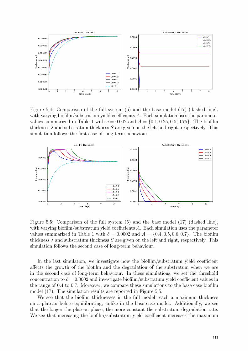
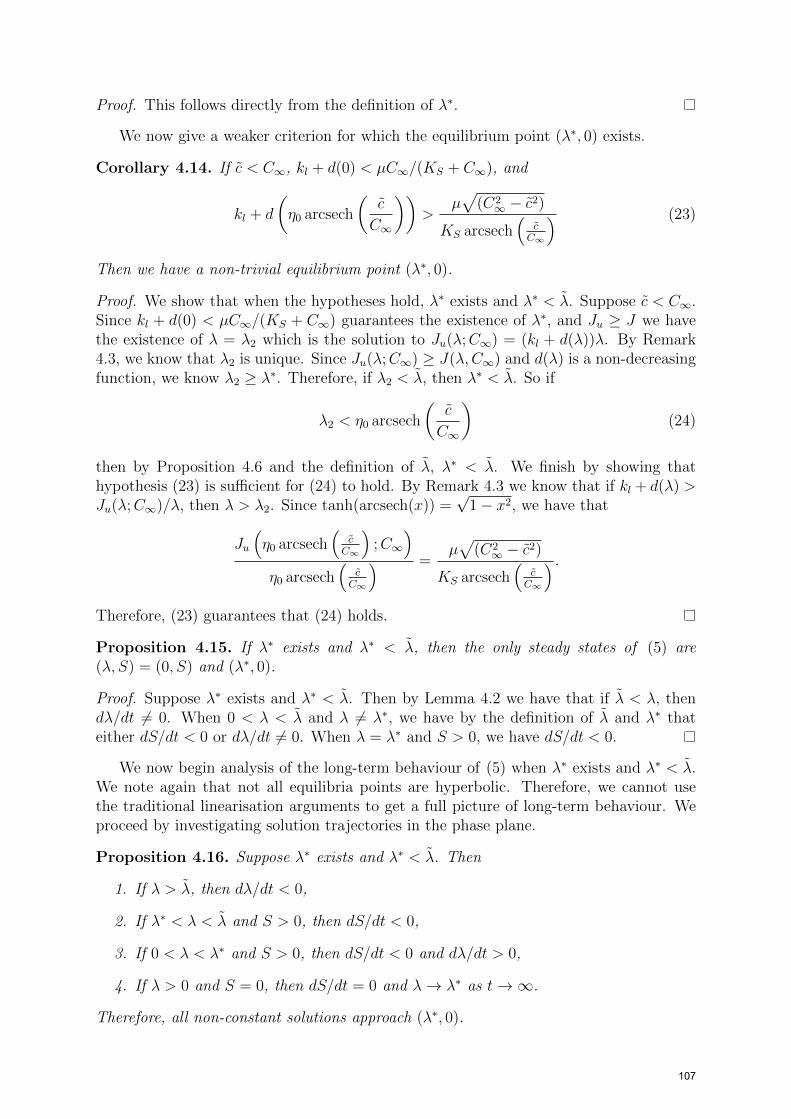
Figure 5.4: Comparison of the full system (5) and the base model (17) (dashed line),with varying biofilm/substratum yield coefficients A. Each simulation uses the parametervalues summarized in Table 1 with c = 0.002 and A = {0.1, 0.25, 0.5, 0.75}. The biofilmthickness λ and substratum thickness S are given on the left and right, respectively. Thissimulation follows the first case of long-term behaviour.

Figure 5.5: Comparison of the full system (5) and the base model (17) (dashed line),with varying biofilm/substratum yield coefficients A. Each simulation uses the parametervalues summarized in Table 1 with c = 0.0002 and A = {0.4, 0.5, 0.6, 0.7}. The biofilmthickness λ and substratum thickness S are given on the left and right, respectively. Thissimulation follows the second case of long-term behaviour.

In the last simulation, we investigate how the biofilm/substratum yield coefficientaffects the growth of the biofilm and the degradation of the substratum when we arein the second case of long-term behaviour. In these simulations, we set the thresholdconcentration to c = 0.0002 and investigate biofilm/substratum yield coefficient values inthe range of 0.4 to 0.7. Moreover, we compare these simulations to the base case biofilmmodel (17). The simulation results are reported in Figure 5.5.

We see that the biofilm thicknesses in the full model reach a maximum thicknesson a plateau before equilibrating, unlike in the base case model. Additionally, we seethat the longer the plateau phase, the more constant the substratum degradation rate.We see that increasing the biofilm/substratum yield coefficient increases the maximum

113

thickness achieved by the biofilm along with the time to equilibrium and the length ofthe plateau phase. The increase in the time to equilibrium is due to the degradation ofthe substratum. As the value of the biofilm/substratum yield coefficient increases, therate of substratum degradation decreases, and thus, the biofilm degrades the substratumfor longer. Furthermore, we can see that these simulations all follow the second case oflong-term behaviour; see Figure 4.2, i.e. λ∗ exists and λ∗ < λ, since the final biofilmthickness is positive and the biofilm thickness achieved a maximum. Lastly, as shown inthe analysis, all final biofilm thicknesses are the same as in the base case model.

6 Conclusion

In this paper, we studied a mathematical model of biofilm growth on a degradable sub-stratum, which is an extension of a simpler model (17) where the biofilm was growingon an inert substratum. The purpose was to study the effect of substratum degradationon such models that permit this. We started with the simple case where substratumdegradation occurs if and only if the bacteria at the biofilm-substratum interface layerare active. With this model, we were interested in investigating whether or not such anextension would yield different system behaviour. We found that the equilibria of thesystem and the stability conditions were the same as in the simpler model, i.e. the ex-tension with substratum degradation produced the same long-term behaviour. However,the time evolution of the system is different. We saw that the biofilm thickness doesnot necessarily grow monotonically, which is different from the growth of the biofilm inthe base case model. Therefore, the addition of substratum degradation in systems thatsatisfy our model assumptions is necessary to describe system behaviour accurately.

The non-monotonic growth of the biofilm thickness in certain simulations leads tointeresting consequences for systems satisfying our model assumptions. For example,suppose we are modelling a reactor where there is a biofilm growing, and these biofilmsdegrade the substratum based on our model assumptions. If we are concerned withsubstrate removal inside the reactor, then if we used the simpler biofilm growth model(17) instead of our model (5) we would see an underestimate in the substrate removal.The underestimate of the substrate removal would be caused by the underprediction ofthe total flux of substrate into the biofilm. Which we can see by considering Figure 5.3and that the flux function J(λ;C∞) is increasing in λ. Therefore, for systems satisfyingour model assumptions, it is necessary to include the effects of substratum degradation.

When considering our biofilm growth model, the only way to change the biofilmthickness in the long-term is to scrape off part of the biofilm. In the context of our model,this would be the increase of the detachment rate d(λ). As we can see from our results inSections 4.1 and 4.2, specifically corollaries 4.10 and 4.14 respectively, an increase in thedetachment rate can cause a change in long-term behaviour, namely from case 1 to case2. This change in long-term behaviour is a reflection of the change in the inactive layerof the biofilm. A thicker biofilm means less dissolved substrate for the bacteria at thebase of the biofilm, which means a larger inactive layer and, in the context of our model,no substratum degradation. This system behaviour reflects biological phenomenon as weexpect a thinner biofilm to have a smaller inactive layer.

While the model is simplified, it still provides beneficial first insight into the effects ofsubstratum degradation on biofilm growth. The simplicity of the model allowed for de-tailed analytical results from existence and uniqueness to equilibria and stability analysis.

114

However, an investigation into different degradation kinetics could prove very useful toour understanding of the interactions between biofilms and the substratum. For specificapplications, one would likely need to adapt the substratum degradation kinetics to fittheir system best, but what we have shown is that the addition of substratum degradationcan have a significant impact on the dynamics of these systems. Thus, when applicable,substratum degradation should be implemented in such models.

There are plenty of biofilm growth models in the literature that investigates biofilmformation/growth on inert substratum in more complex settings. For example, modelsthat account for variable bulk substrate concentration and suspended bacterial flocs [5,9],or models which assume a multi-species biofilm as in [14]. Therefore, a further study ofbiofilm growth on degradable substratum in various settings would also be beneficial tothe understanding of biofilm/substratum interactions.

References

[1] F. Abbas and H. J. Eberl, Investigation of the role of mesoscale detachment rate expressionsin a macroscale model of a porous medium biofilm reactor, Int. J. Biomath. Biostat., 2 (2013),pp. 123–143

[2] F. Abbas, R. Sudarsan, and H. J. Eberl, Longtime behaviour of one-dimensional biofilm modelswith shear dependent detachment rates, Math. Biosci. Eng., 9 (2012), pp. 215–239

[3] U. M. Ascher, R. M. M. Mattheij, and R. D. Russell, Numerical solution of boundary valueproblems for ordinary differential equations, SIAM, Philadelphia, PA, 1995

[4] J. R. Dormand and P. J. Prince, A family of embedded Runge-Kutta formulae, J. Comput.Appl. Math., 6 (1980), pp. 19—26

[5] H. J. Gaebler and H. J. Eberl, A simple model of biofilm growth in a porous medium thataccounts for detachment and attachment of suspended biomass and their contribution to substratedegradation, European J. Appl. Math., 29 (2018), pp. 1110–1140

[6] J. Kierzenka and L. F. Shampine, A BVP solver based on residual control and the Maltab PSE,ACM Trans. Math. Software, 27 (2001), pp. 299—316

[7] I. Klapper, Productivity and equilibrium in simple biofilm models, Bull. Math. Biol., 74 (2012),pp. 2917—2934

[8] Z. Lewandowski and H. Beyenal, Fundamentals of Biofilm Research, CBC Press, Boca Raton,FL, 2007

[9] A. Masic, H. J. Eberl, Persistence in a single species CSTR model with suspended flocs and wallattached biofilms, Bull. Math. Biol., 74 (2012), pp. 1001—1026

[10] Y. G. Maksimova, Microbial biofilms in biotechnological processes, Appl. Biochem. Micro., 50(2014), pp. 750—760

[11] P. Virtanen, R. Gommers, T. E. Oliphant, M. Haberland, T. Reddy, D. Cournapeau,E. Burovski, P. Peterson, W. Weckesser, J. Bright, S. J. van der Walt, M. Brett, J.Wilson, K. J. Millman, N. Mayorov, A. R. J. Nelson, E. Jones, R. Kern, E. Larson, C.Carey, I. Polat, Y. Feng, E. W. Moore, J. VanderPlas, D. Laxalde, J. Perktold, R.Cimrman, I. Henriksen, E. A. Quintero, C. R. Harris, A. M. Archibald, A. H. Ribeiro,F. Pedregosa, P. van Mulbregt, and SciPy 1.0 Contributors, SciPy 1.0: fundamentalalgorithms for scientific computing in Python, Nat. Methods, 17 (2020), pp. 261–272

[12] W. Walter and R. Thompson, Ordinary Differential Equations, Springer, New York, NY, 1998

[13] O. Wanner, H. J. Eberl, E. Morgenroth, D. R. Noguera, C. Picioreanu, B. E.Rittmann, and M. Van Loosdrecht, Mathematical Modelling of Biofilms, IWA Publishing,London, England, 2006

[14] O. Wanner and W. Gujer, A multispecies biofilm model, Biotechnol. Bioeng., 28 (1986), pp. 314—328

115