A manual for - LARSA 4D 4D Reference Manual Self Weight 95 Weight Factor and Gravity Load Directions...
296
Transcript of A manual for - LARSA 4D 4D Reference Manual Self Weight 95 Weight Factor and Gravity Load Directions...


LARSA 4D Reference Manual
A manual for
LARSA 4DFinite Element Analysis and Design Software
Last Revised October 2016
Copyright (C) 2001-2016 LARSA, Inc. All rights reserved. Information in this document issubject to change without notice and does not represent a commitment on the part of LARSA,Inc. The software described in this document is furnished under a license or nondisclosureagreement. No part of the documentation may be reproduced or transmitted in any form or byany means, electronic or mechanical including photocopying, recording, or information storageor retrieval systems, for any purpose without the express written permission of LARSA, Inc.

LARSA 4D Reference Manual
Table of ContentsIntroduction 11
Model Data Reference 13
Properties 17
Materials 19Basic Isotropic Material Properties 19
Other Material Properties for Time Dependent and Inelastic Analyses 19
Sections 21General Section Properties 21
Properties for Time-Dependent Analysis 21
Properties for Inelastic Analysis 22
Stress Recovery Points 22
Section Dimensions 22
Centroid Offset 23
Spring Property Definitions 25Nonlinear Elastic Spring Properties 25
6x6 Stiffness Matrix Properties 25
Inelastic (Hysteretic) Spring Properties 25
Nonlinear Spring Curve 26
Isolator Property Definitions 29
User Coordinate Systems 31The Global Coordinate System 31
Defining Coordinate Systems 31
Cylindrical Coordinate Systems 32
Spherical Coordinate Systems 33
Bridge Paths 33
Bridge Paths 37Bridge Axes 37
Horizontal Geometry 38
Vertical Geometry 39
Superstructure Rotation 40
Time-Dependent Material Property Definitions 41Creep and Shrinkage Properties for CEBFIP-78 41
Creep and Shrinkage Properties for CEBFIP-90 42
Other Properties 42
Material Curves 43
Relaxation Coefficients 43
Geometry 45
Joints 47General Properties 47
Translational and Rotational Degrees of Freedom (DOF) 47
Displacement User Coordinate System 48
3

LARSA 4D Reference Manual
Members 49Member Properties 49
Connection Beam Properties 53
Properties for Time-Dependent Material Effects 53
Member Coordinate Systems (Local Axes) 54
Self-Weight Computation 56
Spans 59
Plates 61Usage Notes 61
Element Formulation 61
Attributes of Plates 62
Plate Local Axes 63
Self-Weight Computation 63
Springs 65Usage Notes 65
Grounded Spring Element 65
Two-Node Spring Element 65
Inelastic (Hysteretic) Spring Element 66
General Attributes 66
Stiffness Attributes 67
Isolators 69
Mass Elements 71
Slave/Master Constraints 73
Tendons 75About the Tendon 75
Friction Losses 75
Anchorage Slip Losses 76
Elastic Shortening of Concrete Losses 76
Other Losses 76
Attributes 76
Path Geometry 77
Example Path 81
Lanes 83Basic Properties 83
Path Geometry 84
Lane Path Example 85
Loads 89
Static Load Cases 91Load Classes for Code-Based Results 91
Load Combinations 93Including Response Spectra Cases 93
Including Moving Load Cases 93
Use in Nonlinear Analysis 93
4
LARSA 4D Reference Manual
Self Weight 95Weight Factor and Gravity Load Directions 95
Self Weight Computation 95
In Staged Construction Analysis 95
Joint Loads 97
Support Displacements 99
Member Loads 101
Member Thermal Loads 103Load Input 103
Nonlinear Thermal Gradient Curves 104
Plate Loads 105Plate Load Fields 105
Point Load Coordinates 106
Moving Loads 107
Influence Loads 109
Time History Loads 111Excitation Functions 111
Initial Conditions 112
Construction Activities 113
Construct and Deconstruct Activities 115Deconstruction 115
Self Weight and Mass 115
Segmental Construction Methods 116
Load Activities 119Creating Load Activities 119
Using Load Activities 119
Self-Weight Load Cases 119
Support and Hoist Activities 121Activity Fields 121
Slave/Master Change Activities 123Activity Fields 123
Tendon Stressing and Slackening Activities 125Activity Fields 125
Displacement Initializations 127What It Does 127
Activity Fields 128
Analysis Scenarios 129
Analysis Reference 131
Static Analysis 135
Linear Static Analysis 137Structure Model for Linear Static Analysis 137
5

LARSA 4D Reference Manual
Analysis Results 137
Assumptions in a Linear Static Analysis 138
P-Delta Analysis 139Using Load Combinations for the P-Delta 139
Caveats 139
Method 139
Convergence Criteria 139
Nonlinear Static Analysis 141Why a Nonlinear Analysis 141
Applications of the Nonlinear Analysis 142
Equations of Equilibrium and Solution 142
Caveats 142
Incremental Loading 143
Convergence Criteria 143
Displacement Convergence and Unbalanced Forces 143
Load Case Data for Nonlinear Static Analysis 144
Nonlinear Buckling Analysis 145Advantages of a Nonlinear Analysis 145
Using the Nonlinear Buckling Analysis 145
Nonlinear Pushover Analysis 147
Nonlinear Static Analysis Options 149
Incremental Nonlinear and Nonlinear Buckling Analysis Options 151
Nonlinear Pushover Analysis Options 153
Eigenvalue Analysis 155
Eigenvalue and Stressed Eigenvalue Analysis 157Unstressed (Standard) Eigenvalue Analysis 157
Stressed Eigenvalue Analysis 157
Response Spectra Analysis 159Response Spectra Curve 159
Modal Damping 159
Modal Combination 160
Spatial Combination 160
Ground Motion Directions 160
Response Spectra Load Cases 161
Caveat About Sign 162
Analysis Options for Response Spectra 162
Eigenvalue Analysis Options 163
Stressed Eigenvalue Analysis Options 165
Time History Analysis 167
Linear Time History Analysis 169Time History Load Cases 169
Applied Loads 169
Nonlinear Time History Analysis 171
6

LARSA 4D Reference Manual
Overview 171
Newmark-Beta with Newton-Raphson 171
Sparse Solver Technology 171
Nonlinear Time History Data 171
Time History Analysis Options 173
Nonlinear Time-History Analysis Options 175Geometric Nonlinearity 175
Live Load Analysis 177
Moving Load Analysis 179Vehicle Paths: Lanes 179
Load Cases for Moving Load Analysis 179
Influence Line & Surface Analysis 181
Influence Analysis Overview and Options 183The Assumption of Linearity 183
The Vehicle Loading Algorithm 183
Performing an Influence Analysis 184
General Loading Parameters 185
Vehicular Loading Options 187
Vehicular Options for the 7.01 Compatible Solution Method 190
Uniform/Patch Loading Options 190
Procedure: Getting Results 190
Suggestions for Influence Analysis 193Suggestions for Speed 193
Influence Surfaces in LARSA 4D Version 7.01 195Design Lane Options 195
Vehicle Type and Placement Options 196
AASHTO LFD Point Loading in LARSA 4D Version 7.01 197
Standard Vehicles 199AASHTO and CALTRANS Vehicles 199
AASHTO Load Patterns for Influence Analysis 199
IRC Load Patterns for Influence Analysis 200
Moving Load Analysis Options 203
Staged Construction Analysis 205
Overview of Staged Construction Analysis 207
Staged Construction Activities 209
Setting Up the Model 211Preparation 211
Creating Activities in the Explorer 212
Creating Activities in the Stage Editor 213
Time Effects on Materials 217Definitions 217
General Options 218
7
LARSA 4D Reference Manual
Load Class Tracking 221Setting up the model 221
The Load Classes of Result Cases 221
Accessing Class-Based Results 222
Staged Construction Analysis Options 223Options for Analysis Scenarios 224
Solver Options 227
Analysis Results Reference 229
Joint Results 231
Joint Displacements 233Definitions 233
Joint Reactions 235Definitions 235
Joint Velocities & Accelerations 237Definitions 237
Camber Adjustment 239Definitions 239
Member Results 241
Member End Forces 243Definitions - General 243
Definitions - When Reported in Global Directions 243
Definitions - When Reported in Local Directions 243
Member Sectional Forces 245Definitions 245
Member Stresses 247Computation of Normal Stresses 247
Definitions 247
Member Displacements 249Definitions 249
Member Plastic Deformation 251Definitions 251
Member Yield and Strains 253Definitions 253
Span Displacements and Forces 255Span Displacements 255
Span Sectional Forces 255
Analyzed Member Loads 257Definitions 257
Plate Results 259
Plate Forces on Center 261Definitions 261
8

LARSA 4D Reference Manual
Plate Forces at Joints - External 263Definitions 263
Plate Forces at Joints - Internal 265Definitions 265
Plate Stresses on Center and at Joints 267Definitions 267
Spring Results 269
Spring Forces 271Local Axial/Local Torsional Springs 271
Translation/Rotation X/Y/Z Directions 271
Spring Deformations 273Local Axial/Local Torsional Springs 273
Translation/Rotation X/Y/Z Directions 273
Spring Yield 275
Connection Beam Yield 277
Tendon Results 279
Eigenvalue Results 281
Modal Frequencies 283Definitions 283
Mode Shapes 285Definitions 285
Modal Reactions and Modal Member/Plate Forces 287
9

LARSA 4D Reference Manual
10

LARSA 4D Reference Manual
Introduction
LARSA 4D is the premier general purpose structural analysis and design software. In use throughout the world,LARSA 4D boasts advanced analytical features, from influence surface based analysis to nonlinear time historyanalysis, and an all-new user interface. LARSA 4D: 4th Dimension, the most advanced program in the LARSA 4Dseries, features staged construction analysis and time-dependent material properties.
Clients have turned to LARSA for over 25 years for their structural analysis needs. The LARSA structural analysisengine was originally developed to perform nonlinear static analysis of structures with large displacements, such assuspension and cable-stayed bridges. But, LARSA has come a long way since it was first available on the VAX super-mini computers decades ago. Today, LARSA 4D has the only truly 3D analysis engine providing all of the toolssegmental bridge and large-scale structures engineers can no longer live without.
This is the LARSA 4D Reference Manual, a part of the series of manuals for LARSA 4D. This manual is split intothree sections. In the first, Model Data, LARSA's element library and model definitions are explained. The secondsection, Analysis Reference, describes how the various types of analysis are performed by the LARSA analysis engineand explains analysis parameters. The last section, Analysis Results, explains how to interpret the results of an analysis.
Separate manuals are available that delve deeper into specific uses of LARSA 4D: staged construction analysis, bridgeanalysis, and pushover analysis. In addition, the User's Guide explains how to use LARSA 4D's user interface, and theSamples and Tutorials manual provides a hands-on method for learning about the program.
11

LARSA 4D Reference Manual
12

LARSA 4D Reference Manual
Part IModel Data Reference
The Model Data Reference details the input data describing the structural geometry, element behavior properties, andloading of the structure.
Properties 17
Materials 19Basic Isotropic Material Properties 19
Other Material Properties for Time Dependent and Inelastic Analyses 19
Sections 21General Section Properties 21
Properties for Time-Dependent Analysis 21
Properties for Inelastic Analysis 22
Stress Recovery Points 22
Section Dimensions 22
Centroid Offset 23
Spring Property Definitions 25Nonlinear Elastic Spring Properties 25
6x6 Stiffness Matrix Properties 25
Inelastic (Hysteretic) Spring Properties 25
Nonlinear Spring Curve 26
Isolator Property Definitions 29
User Coordinate Systems 31The Global Coordinate System 31
Defining Coordinate Systems 31
Cylindrical Coordinate Systems 32
Spherical Coordinate Systems 33
Bridge Paths 33
Bridge Paths 37Bridge Axes 37
Horizontal Geometry 38
Vertical Geometry 39
Superstructure Rotation 40
Time-Dependent Material Property Definitions 41Creep and Shrinkage Properties for CEBFIP-78 41
Creep and Shrinkage Properties for CEBFIP-90 42
Other Properties 42
Material Curves 43
13

LARSA 4D Reference Manual
Relaxation Coefficients 43
Geometry 45
Joints 47General Properties 47
Translational and Rotational Degrees of Freedom (DOF) 47
Displacement User Coordinate System 48
Members 49Member Properties 49
Connection Beam Properties 53
Properties for Time-Dependent Material Effects 53
Member Coordinate Systems (Local Axes) 54
Self-Weight Computation 56
Spans 59
Plates 61Usage Notes 61
Element Formulation 61
Attributes of Plates 62
Plate Local Axes 63
Self-Weight Computation 63
Springs 65Usage Notes 65
Grounded Spring Element 65
Two-Node Spring Element 65
Inelastic (Hysteretic) Spring Element 66
General Attributes 66
Stiffness Attributes 67
Isolators 69
Mass Elements 71
Slave/Master Constraints 73
Tendons 75About the Tendon 75
Friction Losses 75
Anchorage Slip Losses 76
Elastic Shortening of Concrete Losses 76
Other Losses 76
Attributes 76
Path Geometry 77
Example Path 81
Lanes 83Basic Properties 83
Path Geometry 84
Lane Path Example 85
14
LARSA 4D Reference Manual
Loads 89
Static Load Cases 91Load Classes for Code-Based Results 91
Load Combinations 93Including Response Spectra Cases 93
Including Moving Load Cases 93
Use in Nonlinear Analysis 93
Self Weight 95Weight Factor and Gravity Load Directions 95
Self Weight Computation 95
In Staged Construction Analysis 95
Joint Loads 97
Support Displacements 99
Member Loads 101
Member Thermal Loads 103Load Input 103
Nonlinear Thermal Gradient Curves 104
Plate Loads 105Plate Load Fields 105
Point Load Coordinates 106
Moving Loads 107
Influence Loads 109
Time History Loads 111Excitation Functions 111
Initial Conditions 112
Construction Activities 113
Construct and Deconstruct Activities 115Deconstruction 115
Self Weight and Mass 115
Segmental Construction Methods 116
Load Activities 119Creating Load Activities 119
Using Load Activities 119
Self-Weight Load Cases 119
Support and Hoist Activities 121Activity Fields 121
Slave/Master Change Activities 123Activity Fields 123
Tendon Stressing and Slackening Activities 125Activity Fields 125
Displacement Initializations 127
15

LARSA 4D Reference Manual
What It Does 127
Activity Fields 128
Analysis Scenarios 129
16

LARSA 4D Reference Manual
Properties
Property data are specifications of element behavioral properties that are used for one or more elements in the structure.These include materials, sections, nonlinear spring behavior definitions, isolator and bearing property definitions, andtime-dependent material property definitions. User coordinate systems are also defined in this section.
Materials 19Basic Isotropic Material Properties 19
Other Material Properties for Time Dependent and Inelastic Analyses 19
Sections 21General Section Properties 21
Properties for Time-Dependent Analysis 21
Properties for Inelastic Analysis 22
Stress Recovery Points 22
Section Dimensions 22
Centroid Offset 23
Spring Property Definitions 25Nonlinear Elastic Spring Properties 25
6x6 Stiffness Matrix Properties 25
Inelastic (Hysteretic) Spring Properties 25
Nonlinear Spring Curve 26
Isolator Property Definitions 29
User Coordinate Systems 31The Global Coordinate System 31
Defining Coordinate Systems 31
Cylindrical Coordinate Systems 32
Spherical Coordinate Systems 33
Bridge Paths 33
Bridge Paths 37Bridge Axes 37
Horizontal Geometry 38
Vertical Geometry 39
Superstructure Rotation 40
Time-Dependent Material Property Definitions 41Creep and Shrinkage Properties for CEBFIP-78 41
Creep and Shrinkage Properties for CEBFIP-90 42
Other Properties 42
Material Curves 43
17

LARSA 4D Reference Manual
Relaxation Coefficients 43
18

LARSA 4D Reference Manual
Materials
Material property data is for defining the properties for various materials in the structural model. These materialproperties are assigned to members, plates, and tendons.
Material properties most often define linearly elastic behavior; however, when assigned to hysteretic beam elements(page 49), these properties can define inelastic behavior.
Basic Isotropic Material Properties
The behavior of an isotropic material does not depend on the direction of loading or the orientation of the material.Shearing behavior is uncoupled from extensional behavior.
NameA material's name is used to refer to the material throughout the project.
Modulus of ElasticityYoung's Modulus (Elastic Modulus) of the material.
Poisson RatioPoisson ratio of the material. The range from 0.0 to 0.5 is common, but the ratio must be less than 0.50.
Shear ModulusShear Modulus of the material. The Poisson ratio can be calculated using the Young's modulus and shearmodulus. When any two of the Young's Modulus, Poisson ratio, and shear modulus are specified, the third isautomatically calculated.
Unit WeightWeight density (weight per unit volume) of the material. The self-weight of elements in a static analysis and themass due to self-weight in a dynamic analysis are computed using this entry. If the unit weight is not entered(zero), the element is assumed weightless.
Coefficient of Thermal ExpansionThe coefficient of thermal expansion is used when thermal loadings are specified for the structure. If there are
no thermal loads, this field is optional. The unit of this field is x10-6, meaning a value of 6.5x10⁻⁶ should beentered as simply 6.5.
Other Material Properties for Time Dependent and Inelastic Analyses
These fields are used for steel design, time dependent analyses and inelastic elements in nonlinear analyses.
Yield StressThe yield stress is used to compute the plastic moment capacity for beams. The plastic moment capacity iscomputed as the plastic section modulus times the material yield stress. In pushover analysis, element stiffnessis reduced by the Post-Yield to Initial Slope Ratio after this point is reached.
Post-Yield to Initial Slope RatioThis entry defines the slope of the stress-strain curve after the material yields. The field is the ratio of the post-yield stress-strain slope to the pre-yield stress-strain slope.
19

LARSA 4D Reference Manual
Concrete Strength SpecimenThe specimen type used to get the 28 day strength of the material. It can be either cylinder or cube.
Concrete fc28 or Steel FuCompressive strength of concrete at day 28 or ultimate stress for steel. This entry is used in time-dependentstaged construction analysis if the material is concrete. Fu of steel is used in steel design.
Concrete Cement Hardening TypeCement hardening type to be used in a time-dependent analysis. If the material is not subject to creep andshrinkage, select Not Concrete.
Tendon GUTS (Guaranteed Ultimate Tensile Stress)Required data for tendons. This is the guaranteed ultimate yield stress.
Material Time-EffectThis entry determines long-term material time effects, such as relaxation in tendons, creep and shrinkage in aconcrete members and also the elastic modulus variation of the all elements as a function of age, that membersor tendons assigned this material are subject to during the Staged Construction Analysis (page 205) (see TimeEffects on Materials (page 217)). Choices are drawn from time-dependent material property definitions (page 41).A time-dependent material property definition can also be assigned to a member via its section (page 21). Itis invalid to have a member for which both its material and its section have been assigned a time-dependentmaterial property definition.
For More Information, please refer to the following documentation.
• Members on page 49.
• Time Effects on Materials on page 217.
• For help on using spreadsheets, see Using the Model Spreadsheets in LARSA 4D User’s Manual.
20

LARSA 4D Reference Manual
Sections
Section data is for describing the geometric and analytic cross-sectional properties of members. Section properties areassigned to members.
The section property data is arranged in three groups:
General PropertiesThe first group is for the most often used property data in the analysis such as area and inertias.
Stress Recovery PointsThe second group is for stress recovery points, which are the coordinates of the extreme points or edge pointson the section. These points are also used for defining tendon and lane paths.
Section DimensionsThe last group is for physical section dimensions, which is used for graphical rendering and computationof section properties.
All section properties are entered with respect to the reference coordinate system of the member (see Members (page
49)).
General Section Properties
NameA section's name is used to identify the section throughout the project.
Section AreaThe gross cross-sectional area of the section for axial stiffness. Since truss and cable elements have only axialstiffness, the cross-sectional area is the only property needed for truss and cable elements.
Shear Areas
The shear areas Ay and Az are for transverse shear in the xy- and xz-planes of with corresponding transverseshear stiffness as Ay*G and Az*G.
Torsional ConstantTorsional constant is the area moment about the member x-axis for torsional stiffness.
Moment of Inertias Iyy and IzzThese are the area moments of inertia Iyy and Izz about the member local y- and z-axes, respectively. Thesevalues are used for the bending stiffness of beam elements.
Properties for Time-Dependent Analysis
PerimeterThe perimeter of the section. This is used to determine the notional thickness of the section.
Material Time-Effect
21
LARSA 4D Reference Manual
This entry determines long-term material time effects, such as creep and shrinkage in a concrete members andthe elastic modulus variation of the all elements as a function of age, that members assigned this section aresubject to during the Staged Construction Analysis (page 205) (see Time Effects on Materials (page 217)). Choicesare drawn from time-dependent material property definitions (page 41). A time-dependent material propertydefinition can also be assigned to a member via its material (page 19). It is invalid to have a member for whichboth its material and its section have been assigned a time-dependent material property definition.
Properties for Inelastic Analysis
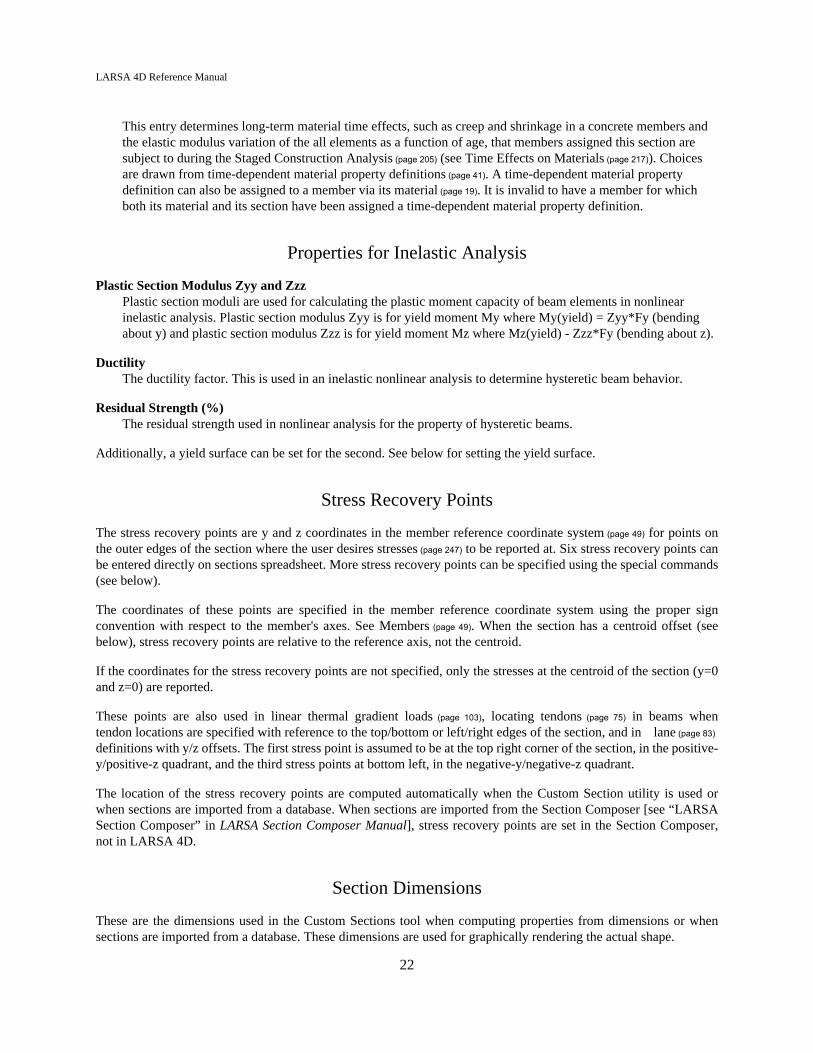
Plastic Section Modulus Zyy and ZzzPlastic section moduli are used for calculating the plastic moment capacity of beam elements in nonlinearinelastic analysis. Plastic section modulus Zyy is for yield moment My where My(yield) = Zyy*Fy (bendingabout y) and plastic section modulus Zzz is for yield moment Mz where Mz(yield) - Zzz*Fy (bending about z).
DuctilityThe ductility factor. This is used in an inelastic nonlinear analysis to determine hysteretic beam behavior.
Residual Strength (%)The residual strength used in nonlinear analysis for the property of hysteretic beams.
Additionally, a yield surface can be set for the second. See below for setting the yield surface.
Stress Recovery Points
The stress recovery points are y and z coordinates in the member reference coordinate system (page 49) for points onthe outer edges of the section where the user desires stresses (page 247) to be reported at. Six stress recovery points canbe entered directly on sections spreadsheet. More stress recovery points can be specified using the special commands(see below).
The coordinates of these points are specified in the member reference coordinate system using the proper signconvention with respect to the member's axes. See Members (page 49). When the section has a centroid offset (seebelow), stress recovery points are relative to the reference axis, not the centroid.
If the coordinates for the stress recovery points are not specified, only the stresses at the centroid of the section (y=0and z=0) are reported.
These points are also used in linear thermal gradient loads (page 103), locating tendons (page 75) in beams whentendon locations are specified with reference to the top/bottom or left/right edges of the section, and in lane (page 83)
definitions with y/z offsets. The first stress point is assumed to be at the top right corner of the section, in the positive-y/positive-z quadrant, and the third stress points at bottom left, in the negative-y/negative-z quadrant.
The location of the stress recovery points are computed automatically when the Custom Section utility is used orwhen sections are imported from a database. When sections are imported from the Section Composer [see “LARSASection Composer” in LARSA Section Composer Manual], stress recovery points are set in the Section Composer,not in LARSA 4D.
Section Dimensions
These are the dimensions used in the Custom Sections tool when computing properties from dimensions or whensections are imported from a database. These dimensions are used for graphically rendering the actual shape.
22

LARSA 4D Reference Manual
The types of dimension measurements for a section vary according to the shape.
Centroid Offset
Sections defined in the Section Composer [see “LARSA Section Composer” in LARSA Section Composer Manual]may not have their COG lined up with the member reference x-axis, which is the joint-to-joint line for the member(plus member end offsets). When this is the case, the section is said to have a centroid offset. In these cases, the memberlocal axes, which are at the COG, do not match the member reference axes. The local axes are used in the placementof member loads (page 101) and in the reporting of member end forces (page 243), sectional forces (page 245), and stresses(page 247). The reference axes, however, are used in the definitions of tendons (page 75) and lanes (page 83).
Additional Commands
Some additional related commands are available. These commands are used to modify input data or to accessadditional attributes of the data referenced above. The commands can generally be accessed in one of several ways.
In the Sections spreadsheet, the commands are available in the Sections menu, or by right-clicking the spreadsheet.Some commands can be applied to more than one row in the spreadsheet at once by selecting multiple rows beforeactivating the command.
The additional commands are as follows:
Calculate Properties
When the section shape and dimensions are given in the Section Dimensions spreadsheet, this commandcomputes the analytic properties of the cross-section based on the shape and dimensions provided. Theproperties computed are: area, Iyy, Izz, J, shear areas, perimeter, and plastic section moduli. This commandmust be activated whenever the shape or dimensions are changed to update the analytic properties.
Edit Parameters
When a section has been imported from the Section Composer, this command brings up a window where thegeometric parameters used to define the section can be viewed and edited. Nonprismatic variation and theanalytic properties at points along the span can also be inspected.
Edit Yield Surface
Opens a spreadsheet to edit the yield surface of the section, which is used to determine the behavior of inelastichysteretic members (page 49). The yield surface is defined by planar surfaces given by the user. The resultingyield surface is the surface of the volume enclosed by the planes. Each plane is given as 1) a vector <a,b,c>normal to the plane and 2) an offset distance d from the origin to the plane, in the direction of the normal vector.This defines the plane ax + by + cz + d = 0. The component a corresponds to the bending moment about thelocal z axis of the member. The component b corresponds to the bending moment about the local y axis of themember. And the component c corresponds to the axial force in the member.
As a simplified example, a cube is made of six planar surfaces with the vectors and offsets shown in the imagebelow.
23

LARSA 4D Reference Manual
Cube-Shaped Yield Surface Definition
More Stress Points
This command is available in the Section Stress Recovery Points spreadsheet and allows the user to entermore than six stress recovery points.
Section Fiber Width vs Depth
This will be used for nonlinear temperature gradients.
Section Fiber Depth vs Width
This will be used for nonlinear temperature gradients.
Rebars
This command opens a spreadsheet to define the rebars present in the section. Rebar information will be usedfor concrete design.
Moment (y) Curvature
For hysteretic connection beam members (see the member element (page 49)), a family of moment-curvaturespring curves can be entered to specify the inelastic behavior of the beam. With this method, the user isresponsible for determining the moment-curvature relation data for the member at different axial loads.Moment curvature relations are entered as spring curve definitions (page 25) with the type field set toMoment curvature. Additionally, the Axial Force field of the spring curve is set to the axial force at whichthe curve is applicable. The Moment (y) Curvature tool opens a spreadsheet where the family of momentcurvature curves for y-moment can be chosen.
Moment (z) Curvature
See the description of the Moment (y) Curvature tool. This tool opens a spreadsheet where the family ofmoment curvature curves for z-moment can be chosen.
For More Information, please refer to the following documentation.
• For help on using spreadsheets, see Using the Model Spreadsheets in LARSA 4D User’s Manual.
• Members on page 49.
• Tendons on page 75.
• LARSA Section Composer in LARSA Section Composer Manual.
24
LARSA 4D Reference Manual
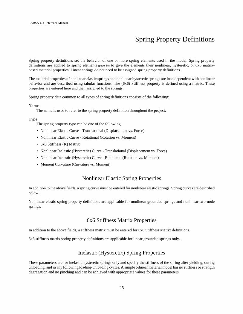
Spring Property Definitions
Spring property definitions set the behavior of one or more spring elements used in the model. Spring propertydefinitions are applied to spring elements (page 65) to give the elements their nonlinear, hysteretic, or 6x6 matrix-based material properties. Linear springs do not need to be assigned spring property definitions.
The material properties of nonlinear elastic springs and nonlinear hysteretic springs are load dependent with nonlinearbehavior and are described using tabular functions. The (6x6) Stiffness property is defined using a matrix. Theseproperties are entered here and then assigned to the springs.
Spring property data common to all types of spring definitions consists of the following:
NameThe name is used to refer to the spring property definition throughout the project.
TypeThe spring property type can be one of the following:
• Nonlinear Elastic Curve - Translational (Displacement vs. Force)
• Nonlinear Elastic Curve - Rotational (Rotation vs. Moment)
• 6x6 Stiffness (K) Matrix
• Nonlinear Inelastic (Hysteretic) Curve - Translational (Displacement vs. Force)
• Nonlinear Inelastic (Hysteretic) Curve - Rotational (Rotation vs. Moment)
• Moment Curvature (Curvature vs. Moment)
Nonlinear Elastic Spring Properties
In addition to the above fields, a spring curve must be entered for nonlinear elastic springs. Spring curves are describedbelow.
Nonlinear elastic spring property definitions are applicable for nonlinear grounded springs and nonlinear two-nodesprings.
6x6 Stiffness Matrix Properties
In addition to the above fields, a stiffness matrix must be entered for 6x6 Stiffness Matrix definitions.
6x6 stiffness matrix spring property definitions are applicable for linear grounded springs only.
Inelastic (Hysteretic) Spring Properties
These parameters are for inelastic hysteretic springs only and specify the stiffness of the spring after yielding, duringunloading, and in any following loading-unloading cycles. A simple bilinear material model has no stiffness or strengthdegregation and no pinching and can be achieved with appropriate values for these parameters.
25
LARSA 4D Reference Manual
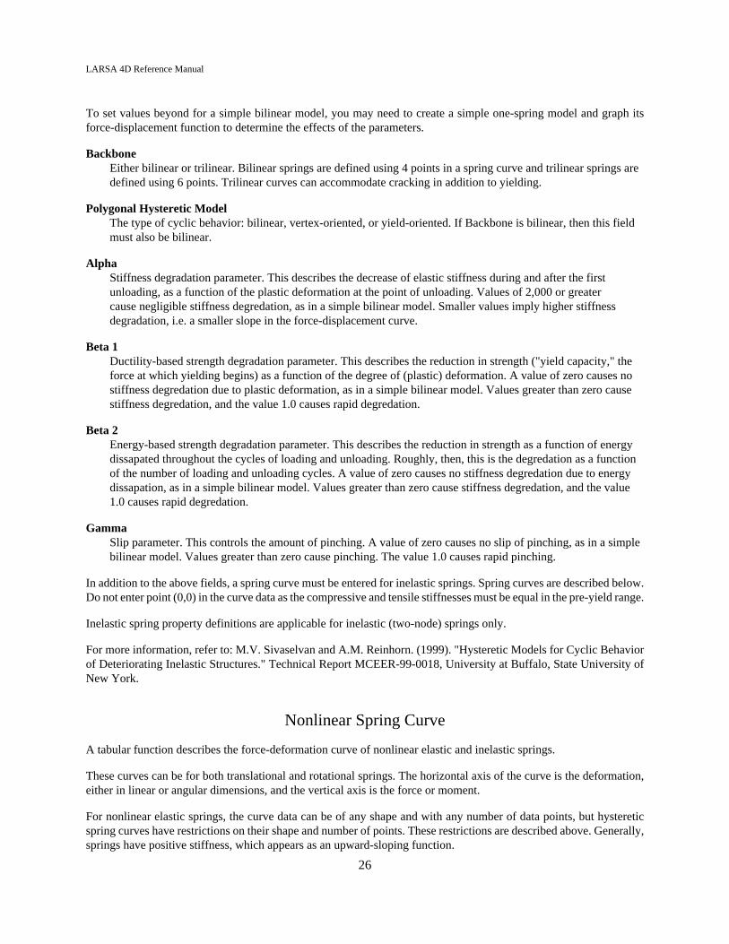
To set values beyond for a simple bilinear model, you may need to create a simple one-spring model and graph itsforce-displacement function to determine the effects of the parameters.
BackboneEither bilinear or trilinear. Bilinear springs are defined using 4 points in a spring curve and trilinear springs aredefined using 6 points. Trilinear curves can accommodate cracking in addition to yielding.
Polygonal Hysteretic ModelThe type of cyclic behavior: bilinear, vertex-oriented, or yield-oriented. If Backbone is bilinear, then this fieldmust also be bilinear.
AlphaStiffness degradation parameter. This describes the decrease of elastic stiffness during and after the firstunloading, as a function of the plastic deformation at the point of unloading. Values of 2,000 or greatercause negligible stiffness degredation, as in a simple bilinear model. Smaller values imply higher stiffnessdegradation, i.e. a smaller slope in the force-displacement curve.
Beta 1Ductility-based strength degradation parameter. This describes the reduction in strength ("yield capacity," theforce at which yielding begins) as a function of the degree of (plastic) deformation. A value of zero causes nostiffness degredation due to plastic deformation, as in a simple bilinear model. Values greater than zero causestiffness degredation, and the value 1.0 causes rapid degredation.
Beta 2Energy-based strength degradation parameter. This describes the reduction in strength as a function of energydissapated throughout the cycles of loading and unloading. Roughly, then, this is the degredation as a functionof the number of loading and unloading cycles. A value of zero causes no stiffness degredation due to energydissapation, as in a simple bilinear model. Values greater than zero cause stiffness degredation, and the value1.0 causes rapid degredation.
GammaSlip parameter. This controls the amount of pinching. A value of zero causes no slip of pinching, as in a simplebilinear model. Values greater than zero cause pinching. The value 1.0 causes rapid pinching.
In addition to the above fields, a spring curve must be entered for inelastic springs. Spring curves are described below.Do not enter point (0,0) in the curve data as the compressive and tensile stiffnesses must be equal in the pre-yield range.
Inelastic spring property definitions are applicable for inelastic (two-node) springs only.
For more information, refer to: M.V. Sivaselvan and A.M. Reinhorn. (1999). "Hysteretic Models for Cyclic Behaviorof Deteriorating Inelastic Structures." Technical Report MCEER-99-0018, University at Buffalo, State University ofNew York.
Nonlinear Spring Curve
A tabular function describes the force-deformation curve of nonlinear elastic and inelastic springs.
These curves can be for both translational and rotational springs. The horizontal axis of the curve is the deformation,either in linear or angular dimensions, and the vertical axis is the force or moment.
For nonlinear elastic springs, the curve data can be of any shape and with any number of data points, but hystereticspring curves have restrictions on their shape and number of points. These restrictions are described above. Generally,springs have positive stiffness, which appears as an upward-sloping function.
26
LARSA 4D Reference Manual
All spring curves must have a point on both sides of (0,0). Hysteretic spring curves prohibit the (0,0) point, as describedabove.
For curves assigned to two-node springs acting in the axial direction, the sign convention is as follows: Extensionsand tensile forces have positive signs; Shortening and compressive forces have negative signs.
For curves assigned to two-node springs acting in the torsional direction, positive displacement corresponds to positiverotation of the end joint relative to the start joint, following the right-hand rule, about the joint-to-joint line.
For curves assigned to two-node springs acting in the translational or rotational x, y, or z directions, positivedisplacement corresponds to positive displacement or rotation of the end joint relative to the start joint in that direction.That is, positive displacement does not necessarily correspond with tension or extension. Rather, it follows the relativedisplacement of the end joint compared to the start joint.
For curves assigned to grounded (i.e. one-node) springs, the sign convention is as follows: Positive displacements willproduce positive forces and negative reactions. That is, if the joint connected to a grounded spring displaces in thepositive-z direction, then the force in the spring will be determined from the positive side of the spring curve.
The stiffness k of a spring in the tangent stiffness matrix is the slope of the curve and varies as a function of thedeformations in the spring. The value is computed in LARSA in the following manner:
• Assume an iteration in nonlinear analysis is performed and joint displacements are known for this iteration.
• Deformation (elongation or rotational deformation) of the element is computed using the nodaldisplacements of the element.
• With deformation known, the spring force is determined from the tabular deformation-force curve assignedas the material property. The table look-up is performed using linear interpolation within the table and linearextrapolation outside the table using the last two end points at the appropriate table end.
• Note that the familiar rule of linear elastic spring FORCE = K x ÐL does not apply to nonlinear springs.
• The stiffness is computed as the slope of the curve corresponding to the computed deformation where x-axisis the deformation.
• The spring force and the new stiffness is used in the next iteration of the nonlinear analysis to establish theunbalanced load vector and tangent stiffness matrix of the structure.
Additional Commands
Some additional related commands are available. These commands are used to modify input data or to accessadditional attributes of the data referenced above. The commands can generally be accessed in one of several ways.
In the Springs spreadsheet, the commands are available in the Springs menu, or by right-clicking the spreadsheet.Some commands can be applied to more than one row in the spreadsheet at once by selecting multiple rows beforeactivating the command.
The additional commands are as follows:
Edit Curve
This command opens a new spreadsheet window where the spring curve can be modified and view as agraph. The curve is entered as a list of points on the curve. The analysis engine will linearly interpolate thecurve to find intermediate values. Special restrictions on the number and positions of the points may applydepending on the curve type (see above).
27

LARSA 4D Reference Manual
Edit Stiffness Matrix
When the spring property type is 6x6 Stiffness Matrix, this command opens a new spreadsheet windowwhere the 6x6 stiffness matrix can be entered. The matrix must be symmetric, so only the upper half of thematrix is editable.
Edit Damping Matrix
When the spring property type is 6x6 Damping Matrix, this command opens a new spreadsheet windowwhere the 6x6 damping matrix can be entered. The matrix must be symmetric, so only the upper half of thematrix is editable.
For More Information, please refer to the following documentation.
• Springs on page 65.
• For help on using spreadsheets, see Using the Model Spreadsheets in LARSA 4D User’s Manual.
28

LARSA 4D Reference Manual
Isolator Property Definitions
Isolator property definitions set the behavior for one or more isolator elements used in the model. These propertydefinitions are assigned to isolator elements (page 69) to give the elements their behavioral properties.
An isolator element has the behavior of a dashpot, such as a viscous damping device. These devices are widely usedas structural protective systems for extreme loading (wind and earthquake) cases. Due to their combined benefits interms of overall displacement reduction and energy dissipation, dampers are considered to be one of the most effectivestructural protective systems.
The dashpot element in LARSA is suitable for modeling the behavior of fluid viscous dampers or other devicesdisplaying viscous behavior. This element can only be used in the time history analysis (and only in the nonlinear timehistory analysis before LARSA 4D version 8.0) because the response of the element is velocity-dependent.
The dashpot is controlled by a damping coefficient C and a velocity power n. The force in the dashpot, F, is a function
of the velocity across the element (v, the difference in velocity at the end joints), where F = Cvn.
Fluid dampers which operate on the principle of fluid orificing, produce an output force which is proportional to thepower of the velocity. That power n can take values in the range of 0.5 to 2.0. This element has linear behavior whenn=1 (but note that the element cannot be used in a linear time history analysis before LARSA 4D version 8.0).
It should be noted that when the velocity exponent n is not 1.0, then the damping coefficient and velocity power mustbe chosen with respect to a particular choice of units. Care should be taken for units of C and v when using nonlineardamping properties.
The following fields are required for dashpot elements:
NameThe name is used to refer to the property definition throughout the project.
ClassCurrently only Dashpot is supported.
Damping CoefficientThe damping coefficient, C, used in time history analysis. The coefficient is in units of force-per-velocity. If theisolator property definition is used on an isolator element whose direction is rotational, the unit is given in unitsof moment per units of velocity.
Velocity PowerThe power that the velocity is raised to, typically in the range of 0.5 to 1.2. If the value is 1.0, then the elementhas linear behavior (see above).
For More Information, please refer to the following documentation.
• Isolators on page 69.
• For help on using spreadsheets, see Using the Model Spreadsheets in LARSA 4D User’s Manual.
29

LARSA 4D Reference Manual
30

LARSA 4D Reference Manual
User Coordinate Systems
User coordinate systems (UCSs) are used to describe the geometry of the structure in alternative coordinate systems andalso to specify the directions of joint degrees of freedom, loads and displacements applied at joints, and the orientationof springs and isolators. There are four types of UCSs: rectangular, cylindrical, spherical, and bridge path.
In most structures, the coordinates of the joints are specified in the Global Coordinate System and joint degrees offreedom, loads and displacements applied at joints, and the orientation of springs and isolators follow the global axes.However, when a user coordinate system is assigned to the Displacement Coordinate System property of a joint (seeJoints (page 47)), then the directions of the joint's degrees of freedom, and loads and displacements applied at thatjoint, are with respect to the user coordinate system. In addition, the orientation of springs (page 65) and isolators (page
69) connected to that joint may be affected.
The use of the additional user coordinate systems is merely a user convenience. The structures with curve beams,tunnels, domes, or structures with inclined supports can be modeled much easier using multiple displacementcoordinate systems. For example, it is more convenient to specify radial and tangential loads or supports on curvedstructures by using a cylindrical rather than rectangular coordinate system.
Coordinate systems can be edited using the Properties spreadsheets or with the Model Data Explorer [see “UserCoordinate Systems” in LARSA 4D User’s Manual].
The Global Coordinate System
The structure model has always one Global Coordinate System. The Global Coordinate system is a rectangularcoordinate system with the axes X, Y and Z. The axes are perpendicular and right-handed. The origin and directionsare chosen arbitrarily by the user, however the direction of the Z-axis is used in interpreting the orientation angle ofmembers.
Defining Coordinate Systems
A user coordinate system definition consists of the following:
TypeThe coordinate system type can be rectangular, cylindrical, spherical, or bridge path. The type of a usercoordinate system affects how coordinates are entered and displayed, but not the location or orientation of theuser coordinate system.
Origin (X/Y/Z)This is the origin of the user coordinate system, in global coordinates.
For rectangular UCSs, the origin is the (0, 0, 0) point in local coordinates; for cylindrical UCSs, this is the centerof the cylinder at z = 0; for spherical UCS, this is the center of the sphere; and for bridge paths, this is the locationof the first point on the path.
In the spreadsheets, the following two fields are used to define UCSs:
Axis Point (X/Y/Z)The vector from the origin to this point defines the positive x-axis of the user coordinate system. The axis pointis specified in global coordinates.
31

LARSA 4D Reference Manual
Point on XY Plane (X/Y/Z)This is a point on the positive-y side of the x-y plane of the user coordinate system, given in global coordinates.It may, of course, be a point on the UCS's +y-axis itself, but it need not be because the y-axis can bedetermined with any point on the +y side of the x-y plane.
The x-axis of the UCS is the vector from the Origin to the Axis Point.
The z-axis of the UCS is determined by taking the normal to the plane defined by the Origin, Axis Point, and Pointon XY Plane.
The y-axis of the UCS is determined by taking the cross product of the z-axis and the x-axis.
The right-hand-rule applies.
Cylindrical Coordinate Systems
Cylindrical Coordinate System
Cylindrical coordinate systems are three-dimensional extensions to polar coordinates. The concentric circles of polarcoordinates are on the x-y plane of the UCS and are extruded through the UCS's z-axis. A cylindrical coordinate hasthe components r, theta, and z. The z-coordinate is the same as when the coordinate is expressed in rectangular form.R and theta are computed as in polar coordinates as if all points are on the x-y plane.
R is the perpendicular distance from a point to the z-axis of the user coordinate system.
Theta is the projected angle from the x-axis to a point, generally expressed in degrees.
Z is the perpendicular distance from a point to the x-y plane.
Cylindrical coordinate systems are often used to restrain joints in radial or tangential directions, or to apply joint loadsin those directions. To apply radial loads, for instance, create a cylindrical UCS and set its origin to the center ofthe circle about which the loads radiate. For each joint on which a radial load will be applied, set its displacementcoordinate system to the cylindrical UCS. Loads applied to these joints will act in the local directions of the UCS,which means the loads x, y, and z components correspond to r, theta, and z. Applying loads with x-components setto 5 will result in loads of magnitude 5 directed radially away from the origin of the UCS. Using the y-componentinstead would produce tangential loads.
32

LARSA 4D Reference Manual
Using a Cylindrical Coordinate System to Apply Radial Loads
Spherical Coordinate Systems
Spherical coordinate systems have coordinates in r, phi, theta form. R and theta are the same as in cylindrical coordinatesystems, the perpendicular distance to the z-axis and angle from the x-axis, respectively.
Phi is the angle between the z-axis vector and the vector from the origin to a point. It is usually expressed in degrees.
Spherical Coordinate System
Bridge Paths
Bridge path coordinate systems are special "traveling" coordinate systems whose axes are station, transverse offset,and elevation. The station axis follows the curved path of the bridge. It is the arc-distance along the center of thepath, like the distance traveled by a car going down the center of a bridge. The station axis is shown as a thick linein the image below.
The tranverse offset axis is perpendicular to the heading of the bridge at any station. That is, it is always theperpendicular distance from a point to the center line of the bridge, in the plane of the bridge. The transverse lines inthe image are lines of the transverse offset axis.
The elevation axis is perpendicular to the station and offset axes, according to the right-hand rule. This axis is shownas the single arrow going up.
33

LARSA 4D Reference Manual
Bridge Path Coordinate Systems
Bridge paths are defined in two planes. Geometry control points at stations along the bridge with their directionalheadings and curve fitting options define the path in the plan or horizontal view. The elevation or vertical path isdefined by a series of elevation control points at stations along the path, with the elevation and grade at each point.The vertical path is parabolically curve-fit.
For more information, see Bridge Paths (page 37).
Additional Commands
Some additional related commands are available. These commands are used to modify input data or to accessadditional attributes of the data referenced above. The commands can generally be accessed in one of several ways.
In the UCSs spreadsheet, the commands are available in the UCSs menu, or by right-clicking the spreadsheet.Some commands can be applied to more than one row in the spreadsheet at once by selecting multiple rows beforeactivating the command.
In the Model Data Explorer, change to the display for UCSs. Then right-click an object to get this list of commands.You can also apply the command to multiple at once by clicking on the first object, then holding the SHIFT key andclicking on the last object, and last right-clicking any of the to get the list of commands.
In the graphics window, activate the Pointer mouse tool from the toolbar, and then right-click an object in thegraphical display to get the list of commands to apply to that object.
The additional commands are as follows:
Edit UCS...
This command opens the UCS editing window. See User Coordinate Systems [in LARSA 4D User’sManual].
Make This the Current UCS
This command sets the UCS to be the active coordinate system. See User Coordinate Systems [in LARSA 4DUser’s Manual].
Make Global System the Current UCS
This command sets the global coordinate system to be the active coordinate system. See User CoordinateSystems [in LARSA 4D User’s Manual].
Move UCS To Joint
34

LARSA 4D Reference Manual
This command lets the user change the origin of a UCS by clicking on a joint in the graphics window. Awindow titled Move UCS to Joint appears. Click a joint to choose a new origin. Otherwise, click Done tocancel choosing a new origin.
Translate UCS in X/Y/Z
After activating this command, the user is prompted for the distance to move the UCS in either the x, y, or zdirections in global coordinates.
Rotate UCS in X/Y/Z
After activating this command, the user is prompted for an angle in degrees to rotate the UCS axes abouteither the x, y, or z global axes.
For More Information, please refer to the following documentation.
• For help on using spreadsheets, see Using the Model Spreadsheets in LARSA 4D User’s Manual.
35

LARSA 4D Reference Manual
36

LARSA 4D Reference Manual
Bridge Paths
Bridge path coordinate systems are special coordinate systems whose axes are station, transverse offset, and elevation.
Like the cylindrical user coordinate system (page 31), the bridge path user coordinate system is a tool of convenience formodeling. Bridge paths are particularly useful in the setup of model geometry because they allow the user to work invery simple coordinates despite any curvature of the structure. This is accomplished by warping the usual x-axis intoa curve that follows the curvature of the bridge. In bridge path UCSs, this is called the station axis, and it is the thickline down the center of the bridge in the image below.
Bridge Path Coordinate Systems
The curvature of the station axis is given by defining the path in two planes. Geometry control points at stations alongthe bridge with their directional headings and curve fitting options define the path in the plan or horizontal view. Theelevation or vertical path is defined by a series of elevation control points at stations along the path, with the elevationand grade at each point.
Bridge path coordinate systems can also be set as the displacement coordinate system of joints in order to change thedirection of supports, springs, and loads to be parallel or perpendicular to the heading of the bridge at the location ofthe joint. This saves the effort of creating a separate rectangular user coordinate system at each pier, for instance, toset the directions of the supports at the piers.
Coordinate systems can be edited using the User Coordinate Systems (page 31) Properties spreadsheets or with the ModelData Explorer [see “User Coordinate Systems” in LARSA 4D User’s Manual].
Bridge Axes
Like the usual x-axis, the station axis is measured in length units. But the station axis is according to arc length. That is,station axis coordinates are distances that a vehicle would travel as it follows the centerline of the bridge. The benefitof this system is that any coordinate (x, 0, 0) is on the centerline of the bridge. Without a bridge path, trigonometricfunctions would be needed to locate points on the centerline.
The second axis of bridge paths is the tranverse offset axis, which is perpendicular to the station axis at any station, inthe horizontal plane. For example, at station 1000 on the curved bridge, two parallel girders 10 units apart are passingthrough. The bridge path coordinates of the girders at this station are (1000, -5, 0) and (1000, 5, 0), regardless of thecurvature at this point.
The elevation axis is always straight up, with the station axis at zero elevation. This is useful for setting coordinatesrelative to a bridge deck. Sometimes it is also useful to set coordinates relative to a ground line, especially when the
37

LARSA 4D Reference Manual
bridge deck's elevation is not constant. In that case it may be helpful to create two bridge path user coordinate systems,both with the same horizontal geometry, but one with elevations set to the elevation of the deck, and the other withelevations set flat to the ground line.
Horizontal Geometry
Station and Heading
Horizontal geometry is set through geometry control points and curve fitting options. Geometry control points set thedirectional heading at stations along the bridge, usually before and after curved segments. For instance, if a bridgegoes through an arc from station 2500, where the bridge is headed toward the east, to station 3000, where the bridgeis headed at N 30° E, two geometry control points are set:
Station Heading2500 03000 N 30 E
Headings can be entered as counter-clockwise degree measures from east, in either decimal format or DMS format.For DMS format, you may omit the symbols, e.g. enter "30 15 5" for 30° 15' 5. You may also enter surveyor notation,such as N 30 15 5 E, for 30.251 degrees from north going toward east.
Horizontal Curve Definition
Curve Types
The segments between each geometry control point are connected by a curve. The options for curve fitting are enteredinto the spreadsheet on the righthand side of the Horizontal Cuve tab. The curve specified in row 1 of that spreadsheetcorresponds to the segment between the points in rows 1 and 2 in the lefthand spreadsheet, and so on.
Three types of curve fitting are available: straight line, cicle, and spiral.
Straight lines are automatically fit between two points that have the same heading.
For circular curve fitting, choose the Largest Arc option. This will choose the radius of curvature automatically basedon the formula R=S/T, where S is the arc-length of the segment and T is the change in heading from the start pointto the end point in radians.
38

LARSA 4D Reference Manual
Choose Circular Arc to specify a particular radius. If the radius is smaller than the largest radius that can fit betweenthe points, the circular segment will be placed symmetrically between two straight line segments on either end of thesegment.
Spirals
Euler spirals (also known as clothoids or Talbot transition spirals) can also be fit between control points. The spiral is asmooth transition between a circular curve and a straight line. Four spiral options are available. “Spiral Off” is used forspirals from straight lines to circular segments. “Spiral On” is used for spirals from circular segments to striaght lines.The mnemonic is getting “on” the highway (i.e. from circular on-ramp to straight highway) or getting “off” the highway(from striaght highway to circular off-ramp). “Right” spirals go clockwise, while “left” spirals go counter-clockwise.
For example, the Spiral Off Right option creates a clockwise spiral between a straight line and a circle.
The radius of curvature at the circular end is computed automatically from the formula R=S/2T, where S is the arc-length if the spiral and T is the change in heading from the start point to the end point in radians.
Vertical Geometry
The vertical geometry of the station axis is determined by a series of elevation control points. Each point specifies astation, the elevation at that station, and the grade of the deck at that station. The elevation is relative to coordinateset as the origin of the user coordinate system (page 31), in the direction of the z-axis of the UCS. If the UCS origin anddirections are left as the default, elevations are measured from the global xy-plane.
Vertical Curve Definition
The grade and elevation are used to fit curves between the elevation control points. Where possible, parabolic curvefitting is used. Parabolic curve fitting is only applicable when a point of intersection exists for adjacent elevationcontrol points. PI points won't exist between elevation control points with the same grade but different elevations, forinstance. In these cases, cubic curve fitting is applied.
Elevation Curve Fitting
39

LARSA 4D Reference Manual
Superstructure Rotation
Rotation of the superstructure can be set using the "Bank Rotation" spreadsheet. Rotations are specified at controlpoints (stations) along the bridge path, and are given in degrees. The degree angle specifies a rotation about the bridge'sstation axis using the right-hand-rule (clockwise rotation).
Rotation values are linearly interpolated between the control points.
The effect of a rotation is to skew the local cross-sectional coordinate system at that point on the bridge path. Thetransverse offset axis is rotated according to the bank rotation angle, but the elevation axis remains vertical. This isshown in the image below, which displays the transverse offset and elevation axes at a particular cross-section on abridge path.
Bank Rotation
Although the coordinate system is skewed for the purposes of model geometry, a non-skewed (orthogonal) coordinatesystem must be used when a bridge path is used as a joint displacement coordinate system or as the reference systemfor compound element forces results. In these cases, the local directions ignore any bank rotation. This is shown asthe "displacement directions" axes in the image.
40
LARSA 4D Reference Manual
Time-Dependent Material Property Definitions
Time-dependent material property definitions are used only in the time-dependent staged construction analysis. Thesedefinitions define both concrete creep and shrinkage as well as steel relaxation behavior.
The use of time-dependent material property definitions depends on what type of material properties they represent.
For Concrete Creep and ShrinkageTime-dependent material property definitions are assigned to materials (page 19) or to sections (page 21) whenthey are used to calculate creep and shrinkage for members (page 49).
For Steel RelaxationTime-dependent material property definitions are assigned to materials (page 19) when they are used tocalculate relaxation for tendons (page 75).
Creep and Shrinkage Properties for CEBFIP-78
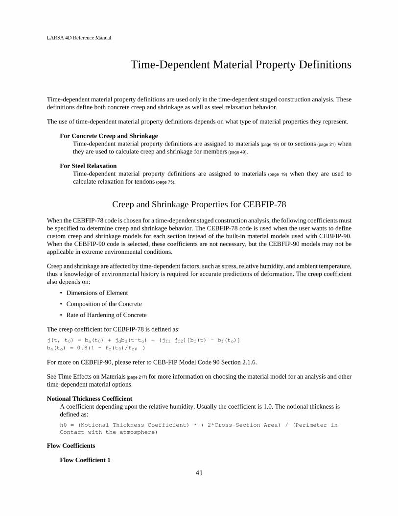
When the CEBFIP-78 code is chosen for a time-dependent staged construction analysis, the following coefficients mustbe specified to determine creep and shrinkage behavior. The CEBFIP-78 code is used when the user wants to definecustom creep and shrinkage models for each section instead of the built-in material models used with CEBFIP-90.When the CEBFIP-90 code is selected, these coefficients are not necessary, but the CEBFIP-90 models may not beapplicable in extreme environmental conditions.
Creep and shrinkage are affected by time-dependent factors, such as stress, relative humidity, and ambient temperature,thus a knowledge of environmental history is required for accurate predictions of deformation. The creep coefficientalso depends on:
• Dimensions of Element
• Composition of the Concrete
• Rate of Hardening of Concrete
The creep coefficient for CEBFIP-78 is defined as:
j(t, t0) = ba(t0) + jdbd(t-to) + (jf1 jf2)[bf(t) - bf(to)]
ba(to) = 0.8(1 - fc(t0)/fc¥ )
For more on CEBFIP-90, please refer to CEB-FIP Model Code 90 Section 2.1.6.
See Time Effects on Materials (page 217) for more information on choosing the material model for an analysis and othertime-dependent material options.
Notional Thickness CoefficientA coefficient depending upon the relative humidity. Usually the coefficient is 1.0. The notional thickness isdefined as:
h0 = (Notional Thickness Coefficient) * ( 2*Cross-Section Area) / (Perimeter inContact with the atmosphere)
Flow Coefficients
Flow Coefficient 1
41

LARSA 4D Reference Manual
jf1. This coefficient is 0.80 for water, 1.00 for very damp atmosphere, 2.00 for outside in general, and 3.00 for avery dry environment
Flow Coefficient 2jf2. Depends on the notional thickness.
The flow coefficients are used in computing the irreversible delayed deformation (flow) which is very muchaffected by the age at which loading commences. Their definitions are in accordance with CEBFIP-78.
LARSA uses the product of these coefficients, jf1 and jf2.
Note: jf1 = 2 and jf2 = 1.4 will represent an average concrete setting and aging in average conditions with a notionalthickness of 0.40m.
Delayed Modulus of Elasticityjd. Used in computing the recoverable part of the delayed deformation (delayed elasticity). It is assumed to beindependent of aging in its development and it is defined by a constant value.
Shrinkage Coefficients
Shrinkage Coefficient 1es1 . Depends on the environment. This coefficient is +0.00010 for water, -0.00013 for very damp atmosphere,-0.00032 for outside in general, -0.00052 for very dry atmosphere.
Shrinkage Coefficient 2es2 . Depends on the notional thickness. This coefficient is usually available in the form of a curve withhorizontal axis as the notional thickness (mm) and vertical axis as the value of for the shrinkage coefficient 2.
The shrinkage coefficient definitions are in accordance with CEBFIP-78.
The strain due to shrinkage which develops in an interval of time (t-t0) is given by
e0 = es1 · es2 (This is the basic shrinkage coefficient.)
es(t, t0) = e0[bs(t) - bs(t0)]
The basic shrinkage coefficient corresponds to EPS in the BC software program.
bs is a user-supplied function corresponding to the change of shrinkage with time depending on the notionalthickness of the section.
The recoverable creep function bd, flow function bf and shrinkage function bs are entered as functions of time (days).The value is computed from the given curve by interpolation. These functions are used in accordance with CEBFIP-78.
Creep and Shrinkage Properties for CEBFIP-90
No values need to be entered when using CEBFIP-90 for creep and shrinkage.
Other Properties
The following other properties can be specified:
Creep Factor
42

LARSA 4D Reference Manual
A factor to apply to the effect of creep for elements to which this time-dependent material property definition isrelevant.
Shrinkage FactorA factor to apply to the effect of shrinkages for elements to which this time-dependent material propertydefinition is relevant.
Relaxation FactorA factor to apply to the effect of relaxation for tendons to which this time-dependent material propertydefinition is relevant.
Material Curves
See Time Effects on Materials (page 217) for more information on which of these curves are needed under differentconditions, choosing the material model for an analysis, and other time-dependent material options.
Concrete Shrinkage Curve (S)Time (in days) versus Strain, the change in shrinkage at this time. A function corresponding to the changeof shrinkage with time, depending on the notional thickness (h0). This curve is only used with CEBFIP-78.This corresponds to the bS function.
Concrete Delayed Plastic Strain Curve (F)Time (in days) versus Plastic Strain. A function corresponding to the development of delayed plasticstrain over time, depending on the notional thickness (h0). This curve is only used with CEBFIP-78. Thiscorresponds to the bF function.
Concrete Delayed Elastic Strain Curve (D)Time (in days) versus Elastic Strain. A function corresponding to the development of delayed elasticstrain over time, depending on the notional thickness (h0). This curve is only used with CEBFIP-78. Thiscorresponds to the bD function.
Time versus Elastic Modulus CurveThis curve is not currently used by LARSA. Instead, a built-in function is applied when called for bychosen code.
Stress/GUTS vs. Relaxation Curve (for Tendons)Relaxation losses for different stress levels in the tendon. This curve is used for all creep and shrinkagecodes. Stress/GUTS is the stress in the tendon divided by the guaranteed ultimate tensile strength. Thisvalue is usually less than 1.0. Higher stress values in the tendon cause higher relaxation losses. Relaxationis the total relaxation. For 6 percent relaxation, specify 0.06.
Time vs. Relaxation Curve (for Tendons)Time (in hours) versus Relaxation (a proportion). A function corresponding to how relaxation varies overtime. This curve is used for all creep and shrinkage codes. If a tendon experiences 100 percent loss ofrelaxation in 1,000 hours, then the value for Time = 1,000 should be 1.0.
Relaxation Coefficients
Relaxation is derived from the product of the coefficients from the Stress/GUTS vs. Relaxation and Time vs. Relaxationcurves. The coefficients are the values of the curves with time being the number of days since the tendon was stressed.
43

LARSA 4D Reference Manual
Additional Commands
Some additional related commands are available. These commands are used to modify input data or to accessadditional attributes of the data referenced above. The commands can generally be accessed in one of several ways.
In the Time Material spreadsheet, the commands are available in the Time Material menu, or by right-clicking thespreadsheet. Some commands can be applied to more than one row in the spreadsheet at once by selecting multiplerows before activating the command.
The additional commands are as follows:
Edit Shrinkage Curve S
This command opens a new spreadsheet window where the S curve can be edited. The use of this curvedepends on the code being used.
Edit Delayed Plastic Strain Curve F
This command opens a new spreadsheet window where the F curve can be edited. The use of this curvedepends on the code being used.
Edit Delayed Elastic Strain Curve D
This command opens a new spreadsheet window where the D curve can be edited. The use of this curvedepends on the code being used.
Edit Curve: Time VS Modulus of Elasticity
This command opens a new spreadsheet window where the time versus modulus of elasticity curve can beedited. The use of this curve depends on the code being used.
Edit Curve: Stress/GUTS VS Relaxation
This command opens a new spreadsheet window where the stress/GUTS versus relaxation curve can beedited. The use of this curve depends on the code being used.
Edit Curve: Time VS Relaxation
This command opens a new spreadsheet window where the time versus relaxation curve can be edited. Theuse of this curve depends on the code being used.
For More Information, please refer to the following documentation.
• For help on using spreadsheets, see Using the Model Spreadsheets in LARSA 4D User’s Manual.
44

LARSA 4D Reference Manual
Geometry
In a finite element analysis, model geometry is defined by the locations of joints, support conditions at joints,constraints between joint degrees of freedom, and a set of elements interconnected at those joints. In addition to generalFEM geometry elements, model geometry includes lanes, tendons, and other miscellaneous objects.
Joints 47General Properties 47
Translational and Rotational Degrees of Freedom (DOF) 47
Displacement User Coordinate System 48
Members 49Member Properties 49
Connection Beam Properties 53
Properties for Time-Dependent Material Effects 53
Member Coordinate Systems (Local Axes) 54
Self-Weight Computation 56
Spans 59
Plates 61Usage Notes 61
Element Formulation 61
Attributes of Plates 62
Plate Local Axes 63
Self-Weight Computation 63
Springs 65Usage Notes 65
Grounded Spring Element 65
Two-Node Spring Element 65
Inelastic (Hysteretic) Spring Element 66
General Attributes 66
Stiffness Attributes 67
Isolators 69
Mass Elements 71
Slave/Master Constraints 73
Tendons 75About the Tendon 75
Friction Losses 75
45

LARSA 4D Reference Manual
Anchorage Slip Losses 76
Elastic Shortening of Concrete Losses 76
Other Losses 76
Attributes 76
Path Geometry 77
Example Path 81
Lanes 83Basic Properties 83
Path Geometry 84
Lane Path Example 85
46

LARSA 4D Reference Manual
Joints
Joints, also known as nodes, are the connection points for stiffness-carrying elements. They are the primary locationswhere displacements are computed. Joints define the physical geometry of the structure and are the sites of supportconditions.
Degrees of freedom are the components of displacement at a joint. Joints can have up to six degrees of freedom,corresponding to translation along the three axes and rotation about the three axes. The number of unrestrained jointdegrees of freedom in a model determines the number of equations to be solved in an analysis.
General Properties
IDNumbers are assigned to joints for identification purposes. They can be any integer, and they must be uniquelyassigned among all joints in a project, but they need not be assigned consecutively.
CoordinatesJoint locations are generally specified using x-, y-, and z-coordinates in the global coordinate system. When auser coordinate system (page 31) is the active coordinate system, then the coordinates are specified with respect tothat coordinate system. (See User Coordinate Systems [in LARSA 4D User’s Manual].)
Translational and Rotational Degrees of Freedom (DOF)
Each degree of freedom can be either free or fixed. A free degree of freedom indicates the joint is free to move, whilea fixed degree of freedom indicates that the joint is not free to move because of the presence of a support.
Without any restraint, the structure will float in space. A free floating structure will have six rigid body degrees offreedom. The structure must be restrained against its rigid body motions. In general, the rule is that degrees of freedomwithout stiffness need to be restrained to prevent rigid body motions as well as ill-conditioning of the system stiffnessmatrix.
For example, 2D structures such as a 2D frame in the xz-plane must have y-translation and x- and z-rotations restrainedfor all joints. To eliminate the rigid body motion at least three additional degrees of freedom must be restrained inthe xz-plane.
The restraint directions are always in the displacement coordinate system of the joint (see below). If the joint is assigneda cylindrical coordinate system as the displacement coordinate system, then X translation represents the radial and Ytranslation represents the tangential motion at the joint.
Universal Restraints [in LARSA 4D User’s Manual] is used to fix a set of degrees of freedom for all joints. Any degreesof freedom restrained universally will apply to all joints, regardless of the DOF selected for a joint.
If the displacement of a joint along any one of its degrees of freedom is known ahead of time, then the degree offreedom is restrained. It should be set to fixed, and a joint displacement load (page 99) should be applied.
Joints can be constrained using Slave/Master Constraints (page 73). Slaved degrees of freedom are removed from thesystem of equations to be solved.
To model other support conditions, such as soil-structure interaction, see Springs (page 65).
47
LARSA 4D Reference Manual
Displacement User Coordinate System
The directions of motion (displacements) of a joint are specified and computed in a coordinate system identified as thejoint displacement coordinate system. The default system is the Global Coordinate System. Any user coordinate system(page 31) (including a Bridge Path Coordinate System) can be assigned to a joint as the displacement coordinate system.
Supports, spring elements, constraints such as slave/masters, joint loads, and support displacements all act in thedirections specified by the joint displacement coordinate system.
Additional Commands
Some additional related commands are available. These commands are used to modify input data or to accessadditional attributes of the data referenced above. The commands can generally be accessed in one of several ways.
In the Joints spreadsheet, the commands are available in the Joints menu, or by right-clicking the spreadsheet.Some commands can be applied to more than one row in the spreadsheet at once by selecting multiple rows beforeactivating the command.
In the graphics window, activate the Pointer mouse tool from the toolbar, and then right-click an object in thegraphical display to get the list of commands to apply to that object only.
To apply the command to multiple joints at once, first select those joints and unselect everything else, then go tothe Modify menu, find the Joints menu, and choose a command from within that menu. Activating these commandsfrom the Modify menu will apply the action to all selected joints.
The additional commands are as follows:
Renumbering Setup
This command sets up renumbering options for joints. The user can choose the starting ID and the step.
Renumber
Renumbers the selected joints according to the renumbering setup options, which must be set first.
For More Information, please refer to the following documentation.
• For help on using spreadsheets, see Using the Model Spreadsheets in LARSA 4D User’s Manual.
• User Coordinate Systems on page 31.
48

LARSA 4D Reference Manual
Members
Members are structural elements connecting two joints and are used to model beams, columns, cables, and trusses.The members can also be used to model yielding connections and plastic hinging within the element.
Member Properties
IDMember numbers are assigned to beams for identification purposes. They can be any integer, and they must beuniquely assigned among all members in a project, but they need not be assigned consecutively.
Start (I) and End (J) JointsA member's connectivity is described using two non-coincident joints. Members may not have zero length. Thejoints' IDs are used here.
Member TypeThe member types that can be selected are Beam, Truss, Cable, Compression-Only Truss, Tension-Only Truss,and Hysteretic Beam. The types Inactive and Construction Line are available to have the analysis engine ignorethe stiffness of the member in the analysis. There is no difference between Inactive and Construction Line, butthe user may decide to make use of the distinction.
Cable, Compression-Only Truss, Tension-Only Truss, and Hysteretic Beam elements and a beam with member-end nonlinear springs are nonlinear elements when used in a nonlinear analysis. If cable or truss elements areused in a linear analysis, they are treated as simple truss elements. The hysteretic beam elements fall back to thestandard beam element in a linear analysis.
Beam Element
The beam element has six degrees of freedom at each end joint: translational displacements in X, Y and Zdirections and rotational displacements about X, Y and Z directions. This element includes axial and sheardeformations, twisting about its x-axis, bending in two perpendicular planes, and associated shears. The beamelement is capable of exactly representing constant axial deformation along the beam with constant torsionalshear deformation and linear bending deformations within the element. This is sufficient for analyzingstructures with loads applied at joint points. However, modeling these deformations requires a higher orderrepresentation due to axial loads, torsional loads, lateral loads, and moments along the elements. Use of thefixed end forces allows these higher-order deformations without the need of additional degrees of freedomfor the beam elements.
This element has geometric nonlinearity and stress-stiffening or softening in all nonlinear analysis types. Italso includes beam-column properties.
When member-end nonlinear springs are assigned, the beam becomes the Connection Beam Element (seebelow).
Truss Element
The truss element has only translational displacements in X, Y and Z directions at each end and it has norotational stiffness. These elements can carry axial force only. The cross-sectional area determines the axialstiffness of the element, and it is the only stiffness required to be entered for sections assigned to trusselement members. The values for Ix, Iy, Iz and shear areas are ignored for truss and cable elements.
49

LARSA 4D Reference Manual
This element has geometric nonlinearity and stress-stiffening or softening in all nonlinear analysis types.
Cable Element
The cable element is identical to the truss element except a cable element cannot resist compressive force.The cable element can only be used in a nonlinear analysis. If during the analysis, the axial force in a cableelement becomes compressive, then the cable element is assumed to have no axial stiffness and cannot carryany load. It is kept in the model as an inactive element with no contributing stiffness. During the loadingprocess of a nonlinear analysis, if the element can become tensile again, it is included in the model withcontributing stiffness to the system.
This element has geometric nonlinearity and stress-stiffening in all nonlinear analysis types.
Compression- and Tension-Only Truss Elements
These elements are identical to the truss element except the compression-only element cannot resist tensionforces and the tension-only element cannot resist compressive forces.
This element has geometric nonlinearity and stress-stiffening or softening in all nonlinear analysis types.This element cannot be used in any linear analysis.
Inelastic Hysteretic Beam Element
This advanced element is used in nonlinear analyses for plastic pushover and progressive collapse. Theformulation of the element is based on spread plasticity to capture the variation of section flexibility andcombine them to determine the element stiffness matrix. It has nonlinear material properties includinghysteretic behavior and geometric nonlinearity for tension stiffening.
Instead of using the material stress-strain relations directly, the hysteretic beam element uses the section axialforce-centroidal strain and moment-curvature relationships to reduce computation. Hence the term strain inthe context of the hysteretic beam element refers to the vector consisting of centroidal axial strain, curvatureabout the element y-axis, and the curvature about the element z-axis.
The interaction between the axial force and the two bending moments at the sections located at the elementGauss points is taken into account using a yield surface and the rules of plasticity: (i) Normal Flow rule and(ii) Kinematic Hardening rule. Normal flow rule states that plastic strain increments are orthogonal to theyield surface. Shear deformations and material nonlinearity in torsion are ignored.
Conventional finite elements use the stiffness formulation where the nodal displacements are interpolatedwithin the element using displacement interpolation functions. In contrast, the hysteretic beam element usesforce interpolation functions, i.e., the element end forces are interpolated within the element. This is because,for beam-elements, while displacement interpolation functions are accurate only for prismatic members withlinear material behavior, the force interpolation functions are always accurate.
This necessitates an element level state determination procedure to determine the element end forces andstrains at the Gauss Points. The Newton-Raphson method is used within the element for this purpose. Thenumber of equations for each hysteretic beam element depends on the number of Gauss points. This numberis set to 10 and cannot be modified by the user.
For the consideration of geometric nonlinearity, the element deformation is split into two parts: (i) the rigidbody rotation of the element coordinate system and (ii) the deformation of the element within this coordinatesystem. Only the former is included in geometric nonlinarity.
50

LARSA 4D Reference Manual
The ignoring of the deformations within the element coordinate system may lead to greater inaccuracieswhen the element is in single curvature and when there is significant deformation before yielding in doublecurvature. In such cases, to increase accuracy the element should be subdivided.
Member loads applied to hysteretic beam elements are non-consistent. These loads are transferredimmediately to the I- and J-joints at the ends of the member. Mid-span point loads, for instance, will betreated instead as split between the end joints.
Connection Beam Element
The connection beam element consists of an elastic beam with built-in yielding springs at the ends. Therecan be up to four such end-springs, two springs at each end, one for each direction of bending. The propertiesof these springs can be assigned so as to model the elastic-plastic behavior of the beam itself and/or to modelthe flexibility and inelastic behavior of the end connections.
The spring properties are assigned using spring curves (page 25) representing the moment-rotation behaviorand by selecting the appropriate parameters that determine hysteretic behavior.
This element is used by specifying member end nonlinear springs for members whose type is beam.
Super Cable Element
The Super Cable Element has multiple internal Gaussian points that simplifies cable modeling. Self-weightand other types of distributed and concentrated loads imposed within the element are analyzed as equivalentconcentrated loads at internal Gaussian points. While simplifying the modeling of cables, the elementprovides a realistic and reliable solution considering geometric nonlinearity due to the sagging effect underarbitrary loading.
Section: At Start, EndThe sectional properties of members are established by assigning a section type (page 21) from the list of sectionsdefined in the project. The section's name is used here.
A member is assigned one or two sections (page 21), which give the cross-sectional properties of the member. Ifone section is assigned, the section applies throughout the member. If two sections are assigned, the sectionalproperties of the member vary linearly, with the start of the member taking sectional properties from the firstassigned section, and the end of the member taking sectional properties from the end of the section.
Sections may have nonprismatic properties, in which the dimensions of the section change over the length of themember, either through assigning two section properties as above, or using a nonprismatic section defined in theSection Composer. When a Section Composer nonprismatic section is assigned to a member, a second sectioncannot also be assigned. When a nonprismatic section from the Section Composer is assigned, use Spans (page
59) to extend the nonprismatic variation over multiple connected members.
The beam element can carry axial forces, shear forces, bending moments and torsion. The data for cross-sectionalarea gives axial stiffness in the x-direction; the torsional moment of inertia gives stiffness for rotation about theelement x-axis; the moment of inertia about the y-axis gives stiffness for translation in the z-direction and forrotation about the y-axis. The moment of inertia about the z-axis gives stiffness for translation in the y-directionand for rotation about the z-axis. The shear areas are for shear deformations. If you set any of the cross-sectionalvariables are set to zero on the section property data, the corresponding stiffness is zero and the correspondingforce at both ends is released.
The orientation of the principal axis of a member is defined with an orientation angle (see below), which sets therelative orientation of the member's local axes. The relation of the principal axis to the local axes of a memberis dependent on the definition of the member's sectional properties.
51

LARSA 4D Reference Manual
MaterialThe material properties of members are established by assigning a material type (page 19). The material's name isused here. Material properties are constant throughout the member, except when a composite section defined inthe Section Composer has been assigned as the section of the member.
Prestress ForceThe initial prestressing force can be set for beam, cable, and truss elements. This type of prestressing can onlybe used in a nonlinear analysis. For prestressing with tendons, see Tendons (page 75). Member loads (page 101)
can also be used.
Rigid Zones
The structural model is normally idealized representing the center line of the beams, columns, and braces. Thistechnique of center-line modeling ignores the thickness of elements and results in greater lengths than is actuallythe case because a portion of element thickness is included in the idealized length of other elements. For instance,the thickness of a column is not accounted for in the lengths of beams attached to the column.
When the joint thickness is small compared to the actual member length, errors due to ignoring the thickness areinsignificant. If the joint thickness is large compared to the actual member length, the error may be significant.
Rigid end zones can be specified to include the actual characteristics of the element end condition. A rigid end isspecified as the length along the member from the start or end joint, or both, which is to be considered infinitelystiff, specified normally as a relative length from zero (i.e. no rigid end) to 0.5 (i.e. half the length of the memberis rigid). It is also possible to specify rigid zones in absolute length units. See the Additional Commands sectionbelow.
Use of rigid end zones produces more realistic displacements and element forces. The element loads areconsidered to be acting only on the elastic length of the beam. The moment and shear force distribution along themember is computed accordingly. Loads placed in rigid zones are ignored.
While the total member length for the purposes of self-weight computation is from joint to joint, the memberlength used in stiffness computation is the length of the elastic portion of the member (i.e. excluding the rigidzones). To shorten the length of the member for the purposes of automatic self-weight computation, use EndOffsets.
Orientation AngleMembers can be situated in any angle about their centroidal axis, such as placing flanges horizontal or vertical.The orientation angle of a member determines this angle. It is crucially important to define the memberorientation properly so that the strong axis of the member is in the right direction.
The orientation angle is used to determine the orientation of the local coordinate system of the member, whichis explained below. Roughly speaking, the orientation angle sets the angle between the global Z-axis and themember's local z-axis. Member sectional properties are given in member local directions. A member whosesection's Izz is greater than its Iyy, which is the case for standard I-shape sections, has its strong axis in its localz-axis direction. If the global Z-axis is "up" and the member is a horizontal beam, the the strong axis needs tobe made horizontal by specifying an orientation angle of 90 degrees. For vertical members, the orientation anglespecifies the angle between the global X-axis and the local z-axis.
See the section on member coordinate systems below for a detailed explanation of member local axes and theorientation angle.
End Offsets
52

LARSA 4D Reference Manual
The centerline of a member is normally the straight line between the member's two joints. End offsets can beapplied to move the end-points of the member, relative to the locations of the joints. Offsets can be applied at thestart and end of a member and are given in global coordinate system directions.
The actual length of the member is computed after the end offsets are applied. This length is used for stiffnesscomputation and load application (including self-weight).
An end offset is equivalent to a rigid link between the offsetted end of the member and the joint it is connectedto at that end.
See the section on member coordinate systems below.
End Releases
The end connections of beam elements are by default perfectly rigid. Beam-joint connections can be also specifiedas pinned or semi-rigid. If a member end release is specified, then the corresponding force is set to zero. Theeffect of the hinge is to free the force at the end of the beam, not at the joint.
The release components are in the member local coordinate system. All directions except Fy and Fz may bereleased. Semi-rigid releases can be applied only for My and Mz. The semi-rigid end connections are specifiedas a percent of fixity. A value of 0 represents a perfect hinge (free) and 100 represents full fixity. Semi-rigidconnections are ignored when applied to hysteretic and connection beams. Fy and Fz can be effectively releasedby making use of slave/master constraints (page 73).
Note that a ridid/fixed member-joint end connection does not prevent the joint itself from translating or rotating,subject to its own degrees of freedom restraint conditions. Instead, a fixed member-joint connection ensures thatall other member rigidly connected to the same joint undergo the same displacement at the joint.
Structure/Construction GroupStructure groups can be assigned directly to members. It is possible to select an existing structure group hereor specify a new one. Structure groups are used to modularize the geometry of the model and plays a key rolein staged construction analysis. For more information see Structure Groups Explorer [see “Structure GroupsExplorer” in LARSA 4D User’s Manual].
Connection Beam Properties
Member End Nonlinear SpringsApplication of these springs makes the member a connection beam element. The connection beam elementconsists of an elastic beam with built-in yielding springs at the ends. There can be up to two springs at eachend, one for each direction of bending. The properties of these springs can be assigned so as to model theelastic/plastic behavior of the beam itself and/or to model the inelastic behavior of the end connections. Thetype of connection beam members must be beam.
Properties for Time-Dependent Material Effects
In the Time-Dependent Staged Construction Analysis (page 205), members can be subject to time-dependent materialeffects including creep, shrinkage, and the time-effect on elastic modulus. The following fields are relevant to thisanalysis:
Casting Day
53

LARSA 4D Reference Manual
The day the member is cast, for use in the Time-Dependent Staged Construction Analysis (page 205). The age ofthe member when constructed is determined by subtracting the casting day from the day of construction set forthe construction stage being analyzed. The casting day of a member must be less than the day of constructionwhen the member is assembled.
Starting in LARSA 4D version 7.2, there is also a cast concrete activity [see “Cast Concrete Activities” in ] inStaged Construction Analysis which can be used to set the casting day of the member. It is also possible to castindividual shapes within a built-up section created in the Section Composer. In this case, the cast concrete stagedconstruction activity must be used rather than the Casting Day attribute of the member element as a whole.
Additionally, a time-dependent material property definition (page 41) must be assigned to either the material or the sectionthat is assigned to the member, but not both. The time-dependent properties are thus indirectly associated with themember element.
Member Coordinate Systems (Local Axes)
Members have two "local" coordinate systems for the purposes of the alignment of cross-section geometry andproperties, loading, the alignment of tendons and lanes, and reporting forces, stresses, and other results. The localcoordinate systems of members determine both the location of the member centroid and the orientation of a memberabout its centroid: which way the wedges and flanges are pointing, for instance. Because these coordinate systemsdefine the position of the centroid and the orientation of the member's strong axis, it is crucially important to understandand set up these systems properly.
The two systems are the reference coordinate system and the local coordinate system. In most cases, the two systemsare the same. They differ only when a member has been assigned a section from the Section Composer [see “LARSASection Composer” in LARSA Section Composer Manual] with a centroid offset from the reference coordinate system.
The reference coordinate system is used to determine the placement of the member's cross-sectional geometry andtendons (page 75). Its origin is located at the I-Joint of the member, plus any end offset specified at the I-Joint. Thex-axis of the reference coordinate system is directed toward the J-Joint of the member, plus any end offset specifiedat the J-Joint.
Member Reference Axes - Alignment With Joints
The y- and z-axes of the reference coordinate system are oriented according to the orientation angle of the member,as follows:
The direction of the reference coordinate system z-axis is determined as follows:
Call the global coordinate axes X, Y, Z and the reference member axes x, y, z. The orientation angle is definedas follows:
• Let A be a plane containing the reference x-axis and a line parallel to the global Z-axis. Plane A will thereforebe perpendicular to the XY plane.
54

LARSA 4D Reference Manual
• Let z' be a point on a line connected to the origin of the reference coordinate system in the plane A andperpendicular to the reference x-axis. The location of z' must be taken so that the projection of the line fromreference origin to z' is in the positive Z direction.
• Then, the orientation angle is defined as the angle from z' to z, positive by the right-hand rule about the memberlocal x-axis.
In other words, the orientation angle is the angle between the global Z-axis and the reference z-axis
Member Reference Axes - Horizontal Members
This definition is valid for all members except when the reference x-axis is parallel to the global Z-axis. Insuch a case, the plane A cannot be defined as described above. If the reference x-axis is parallel to the globalZ-axis, the following rules are used:
• When the reference x-axis is in the same direction as the global Z-axis, the orientation angle is defined as theangle from the minus X-axis to the z-axis.
• When the reference x-axis is in the direction opposite to the global Z-axis, the orientation angle is defined asthe angle from positive X-axis to the z-axis.
Member Reference Axes - Vertical Members
The member local coordinate system x-axis corresponds to the member centroid, with the y- and z-axes the axesabout which the sectional properties (page 21) Iyy and Izz are given and the directions in which member loads (page 101)
and results such as Member End Forces (page 243) are entered and reported in. For standard sections (i.e. those notcreated in the Section Composer), the local x-axis (i.e. the centroid of the member) is placed along the x-axis of thereference coordinate system, and the member local coordinate system coincides with the reference coordinate system.
Note that the local member axes are not necessarily principal axes. If the product of inertia Iyz is zero for the member,the local axes coincide with the principal axes of the member.
For sections created in the Section Composer [see “LARSA Section Composer” in LARSA Section Composer Manual]when the centroid of the section is not placed at the member reference coordinate system origin, the centroid is offsetfrom the reference axis according to the section definition. For sections without nonprismatic variation, this merely
55
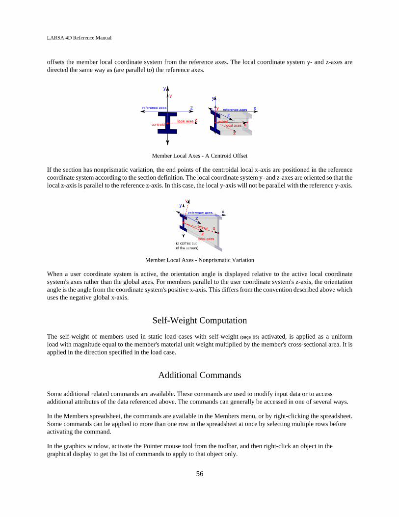
LARSA 4D Reference Manual
offsets the member local coordinate system from the reference axes. The local coordinate system y- and z-axes aredirected the same way as (are parallel to) the reference axes.
Member Local Axes - A Centroid Offset
If the section has nonprismatic variation, the end points of the centroidal local x-axis are positioned in the referencecoordinate system according to the section definition. The local coordinate system y- and z-axes are oriented so that thelocal z-axis is parallel to the reference z-axis. In this case, the local y-axis will not be parallel with the reference y-axis.
Member Local Axes - Nonprismatic Variation
When a user coordinate system is active, the orientation angle is displayed relative to the active local coordinatesystem's axes rather than the global axes. For members parallel to the user coordinate system's z-axis, the orientationangle is the angle from the coordinate system's positive x-axis. This differs from the convention described above whichuses the negative global x-axis.
Self-Weight Computation
The self-weight of members used in static load cases with self-weight (page 95) activated, is applied as a uniformload with magnitude equal to the member's material unit weight multiplied by the member's cross-sectional area. It isapplied in the direction specified in the load case.
Additional Commands
Some additional related commands are available. These commands are used to modify input data or to accessadditional attributes of the data referenced above. The commands can generally be accessed in one of several ways.
In the Members spreadsheet, the commands are available in the Members menu, or by right-clicking the spreadsheet.Some commands can be applied to more than one row in the spreadsheet at once by selecting multiple rows beforeactivating the command.
In the graphics window, activate the Pointer mouse tool from the toolbar, and then right-click an object in thegraphical display to get the list of commands to apply to that object only.
56

LARSA 4D Reference Manual
To apply the command to multiple members at once, first select those members and unselect everything else, thengo to the Modify menu, find the Members menu, and choose a command from within that menu. Activating thesecommands from the Modify menu will apply the action to all selected members.
The additional commands are as follows:
Edit Section
When the member is assigned to a standard section, this command opens the sections spreadsheet to themember's section. When the member is assigned a nonprismatic section, this command opens a new windowto edit the parameters of the section and to view its nonprismatic variation.
See Section Stresses
When analysis results are available and there is an active result case, this command opens a new windowshowing the stresses throughout the member's cross-section, at any point along the length of the member.
Member Section Stresses
Rotate Principal Axis
The member's orientation angle is increased by 90 degrees.
Enter Relative Positions
Choosing this option sets the rigid zone fields to be entered in relative dimensions, where 0 is no rigid zoneand 1 is the entire length of the member.
Enter Absolute Positions
Choosing this option sets the rigid zone fields to be entered in true length dimensions.
Break Member to Existing Joints
If the member passes through joints but is not connected to the joints, the member is broken into pieces sothat it connects to each joint it passes through.
Reverse Direction
The member's start (I) and end (J) joints are reversed, which reverses the direction of the local x-axis of themember.
Select Chain
This command starts with the chosen member, or the selected members, and selects all members on the samechain. A chain is a series of members connected by joints all going in the same direction, like a physicalmember or girder modeled as many members.
Orient Principal Axis to Joint...
This command prompts the user to choose a joint, and then orients the member's local z-axis so that it pointstoward the chosen joint.
Renumbering Setup
57

LARSA 4D Reference Manual
This command sets up renumbering options for members. The user can choose the starting ID and the step.
Renumber
Renumbers the selected members according to the renumbering setup options, which must be set first.
Renumber Chain
This command renumbers the members in the chosen member's chain according to the renumbering options.If the member is selected, only selected members on the chain will be renumbered. Otherwise, all memberson the chain will be renumbered.
Span Properties
If the member is part of a span (page 59), the span's properties are shown.
For More Information, please refer to the following documentation.
• Spans on page 59.
• For help on using spreadsheets, see Using the Model Spreadsheets in LARSA 4D User’s Manual.
• Joints on page 47.
• Materials on page 19.
• Sections on page 21.
• Member Reference Line and Local Coordinate System in LARSA Section Composer Manual.
58

LARSA 4D Reference Manual
Spans
Spans are special entities that represent physical members in the real world. Spans are collections of one or moremembers that usually form a straight line. They must be used in certain cases of sections with nonprismatic variation.
A beam in the real world must often be modeled as multiple members in LARSA so that connections along the membercan be made. Such members are called analytical members, as opposed to physical members, because they only existfor the sake of the analysis.
It is sometimes necessary to treat groups of members that represent one physical member in a special way, such as forcode checks and design [see “Steel Design” in LARSA 4D User’s Manual], for obtaining analysis results (page 255), orwhen the physical member's cross-section has nonprismatic variation [see “Nonprismatic Variation” in LARSA SectionComposer Manual].
All members in a span must have the same section and material properties and must be of the same type. For moreinformation on span properties, see member properties (page 49).
Additional Commands
Some additional related commands are available. These commands are used to modify input data or to accessadditional attributes of the data referenced above. The commands can generally be accessed in one of several ways.
In the Spans spreadsheet, the commands are available in the Spans menu, or by right-clicking the spreadsheet.Some commands can be applied to more than one row in the spreadsheet at once by selecting multiple rows beforeactivating the command.
The additional commands are as follows:
Properties
This command opens a window which allows the user to add and remove members from the span, and tochange the span's material and section properties.
For More Information, please refer to the following documentation.
• For help on using spreadsheets, see Using the Model Spreadsheets in LARSA 4D User’s Manual.
• Members on page 49.
• Steel Design in LARSA 4D User’s Manual.
• Nonprismatic Variation in LARSA Section Composer Manual.
59

LARSA 4D Reference Manual
60

LARSA 4D Reference Manual
Plates
The plate is a planar element with constant thickness, either triangular or quadrilateral in shape, with isotropic materialproperties. It has both plate bending (out-of-plane action) and plane stress (membrane actions, in-plane action) stiffness.
Usage Notes
The plate element is a linear element with linear material properties (page 19). Geometric nonlinearity is only introducedthrough the updating of the deformed shape that occurs in the nonlinear static analysis (but not in Staged ConstructionAnalysis).
The use of the triangular element should be limited to transition zones where quadrilateral elements cannot be easilyused. Triangular elements with interior angles close to 60 degrees each are ideal, and interior angles in excess of 120degrees will distort results around the element.
The aspect ratio for quadrilateral plates, defined as width-to-length, should not be so large as to skew the element. Theinterior angles for quadrilateral elements should not be much greater than 90 degrees.
Plates must have non-zero area and thickness. When the thickness is large in comparison to the width of the plate, athick-plate element behavior must be chosen.
Element Formulation
The user has the ability to choose the plate and membrane behavior of the element separately (starting in LARSA4D version 7.1.13). A shell element is a plate element with both plate and membrane behavior. Except for the classicelement behaviors, all plate behaviors are compatible with all membrane behaviors.
Plate (Out-of-Plane) Action
The following plate behavior formulations are available. Plate behavior adds stiffness in one translational and tworotational degrees of freedom at each joint.
InactiveThe element has no plate stiffness.
ClassicThe classic plate behavior was the only plate element formulation available in LARSA 4D through version7.1.12. A cubic polynomial is used to describe the displacement of the mid-plane. This plate behavior isrecommended for thin plates when shear deformations are negligible. In version 7.1.13 and later, it canonly be used with the classic membrane formulation. Time-dependent material effects such as creep andshrinkage are not supported.
Thin (Discrete Kirchoff Thin Plate)This plate behavior is an alternative to the classic plate behavior which can be used with the bilinear orwith-drilling-DOF membrane behavior. Like the classic plate behavior, it is suitable for plates with smallthickness relative to their width.
61

LARSA 4D Reference Manual
Thick (PQ3/PQ2)This plate behavior should be used when shear deformations and shear force are important such as in deepfoundations, or when the plate thickness is large relative to the plate width. It should be avoided in coarsemeshes or when a point load is applied to a joint. This element is versatile in the analysis of both thick andthin plates, as well as skewed plates, and takes into account shear deformations. It provides a more reliablerepresentation of the three-dimensional solution. The PQ3 formulation is used for quadrilateral elements,while the PQ2 formulation is used for triangular elements.
Membrane (In-Plane) Behavior
The following in-plane membrane behaviors are available:
InactiveThe element has no membrane stiffness.
ClassicThis behavior has no stiffness for rotation about the axis perpendicular to the element surface. It is anincompatible element (bilinear shape functions with incompatible modes). For triangular elements, aconstant strain formulation is used. The classic membrane behavior was the only membrane elementformulation available in LARSA 4D through version 7.1.12. In version 7.1.13 and later, it can only beused with the classic plate formulation. Time-dependent material effects such as creep and shrinkage arenot supported.
Bilinear / CSTFor quadrilateral elements, a bilinear membrane behavior, which is a compatible formulation. Fortriangular elements, a constant strain formulation is used. Like the classic membrane, the bilinear / CSTmembrane has no stiffness for rotation about the axis perpendicular to the element surface.
With Drilling DOFQuadrilateral elements only. This membrane behavior is a separate formulation based on Ibrahimbegovic,Wilson and Taylor’s element which includes drilling degrees of freedom at each node. The drilling DOFmembrane behavior should be used when frame and shell elements are used together and the membraneaction couples with the bending of the frame element (e.g. a beam joining to a wall). For triangularelements, the CST membrane behavior is used instead.
In LARSA 4D prior to version 7.1, the user has the option between plate (classic plate behavior, no membranebehavior), membrane (classic membrane behavior, no plate behavior), or shell (classic plate and membrane behavior).In LARSA 4D version 7.1.00 through 7.1.12, an additional option called thick shell was added which had thick platebehavior and classic membrane behavior.
The same thickness is used for both the plate and membrane behavior.
Attributes of Plates
IDPlate numbers are assigned for identification purposes. They can be any integer, and they must be uniquelyassigned among all plates in a project, but they need not be assigned consecutively.
Plate TypeThe plate behavior, as described above. (Prior to LARSA 4D 7.1.13, only a single Type field was available.)
Membrane Type
62
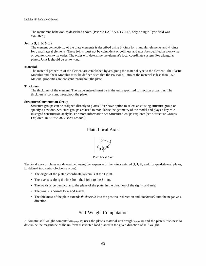
LARSA 4D Reference Manual
The membrane behavior, as described above. (Prior to LARSA 4D 7.1.13, only a single Type field wasavailable.)
Joints (I, J, K & L)The element connectivity of the plate elements is described using 3 joints for triangular elements and 4 jointsfor quadrilateral elements. These joints must not be coincident or collinear and must be specified in clockwiseor counter-clockwise order. The order will determine the element's local coordinate system. For triangularplates, Joint L should be set to none.
MaterialThe material properties of the element are established by assigning the material type to the element. The ElasticModulus and Shear Modulus must be defined such that the Poisson's Ratio of the material is less than 0.50.Material properties are constant throughout the plate.
ThicknessThe thickness of the element. The value entered must be in the units specified for section properties. Thethickness is constant throughout the plate.
Structure/Construction GroupStructure groups can be assigned directly to plates. User have option to select an existing structure group orspecify a new one. Structure groups are used to modularize the geometry of the model and plays a key rolein staged construction analysis. For more information see Structure Groups Explorer [see “Structure GroupsExplorer” in LARSA 4D User’s Manual].
Plate Local Axes
Plate Local Axis
The local axes of plates are determined using the sequence of the joints entered (I, J, K, and, for quadrilateral plates,L, defined in counter-clockwise order).
• The origin of the plate's coordinate system is at the I joint.
• The x-axis is along the line from the I joint to the J joint.
• The z-axis is perpendicular to the plane of the plate, in the direction of the right-hand rule.
• The y-axis is normal to x- and z-axes.
• The thickness of the plate extends thickness/2 into the positive-z direction and thickness/2 into the negative-zdirection.
Self-Weight Computation
Automatic self-weight computation (page 95) uses the plate's material unit weight (page 19) and the plate's thickness todetermine the magnitude of the uniform distributed load placed in the given direction of self-weight.
63

LARSA 4D Reference Manual
Additional Commands
Some additional related commands are available. These commands are used to modify input data or to accessadditional attributes of the data referenced above. The commands can generally be accessed in one of several ways.
In the Plates spreadsheet, the commands are available in the Plates menu, or by right-clicking the spreadsheet.Some commands can be applied to more than one row in the spreadsheet at once by selecting multiple rows beforeactivating the command.
In the graphics window, activate the Pointer mouse tool from the toolbar, and then right-click an object in thegraphical display to get the list of commands to apply to that object only.
To apply the command to multiple plates at once, first select those plates and unselect everything else, then go tothe Modify menu, find the Plates menu, and choose a command from within that menu. Activating these commandsfrom the Modify menu will apply the action to all selected plates.
The additional commands are as follows:
Renumbering Setup
This command sets up renumbering options for plates. The user can choose the starting ID and the step.
Renumber
Renumbers the selected plates according to the renumbering setup options, which must be set first.
Reverse Joint Order
The order of the I, J, K, and L joints are reversed. The effect is to keep the origin of the plate's local axes atthe I joint, but to direct the local x-axis not toward the second joint but instead toward the last joint, and toreverse the direction of the local z-axis.
Shift Joint Order
The order of the I, J, K, and L joints are shifted so that the origin of the plate's local axes moves to the J-joint.
Put Local Axes in Same Direction
When many plates are selected, this command ensures that all of the plates' local z-axes are directed in thesame direction, i.e. all up or all down.
Break Plates to Existing Joints
The plate is meshed so that any joints within the plate are connected to the meshed surface.
For More Information, please refer to the following documentation.
• For help on using spreadsheets, see Using the Model Spreadsheets in LARSA 4D User’s Manual.
• Materials on page 19.
• Joints on page 47.
64

LARSA 4D Reference Manual
Springs
The spring is a very general element that can be used to model foundations, soil-structure interaction, gaps, bearings,and isolators, and it can be used as a general stiffness element. The spring element can be grounded (one-node) or two-node and can have linear, nonlinear, elastic, and inelastic material properties. All springs have one degree of freedomat the joints they are connected to, except when a 6x6 matrix is assigned to the spring.
Usage Notes
For coupled springs, see Isolators (page 69).
The spring element is weightless. Joint loads (page 97) for static analysis or mass elements (page 71) for dynamicanalysis can be used to model the weight or mass of springs, if necessary.
Grounded Spring Element
The grounded spring element (i.e. the one-node spring) is defined using a single joint and there is no length associatedwith the element. The element represents a spring connecting a joint in the structure to the ground at its undeformedlocation.
The linear grounded spring element has the same stiffness in both tension and compression. Either a single springconstant is specified, or a 6x6 stiffness matrix (page 25) is applied to the spring. If a spring constant is given, the elementcan act in one direction only: either translation along or rotation about an axis of the global coordinate system, or thejoint displacement directions (page 47) assigned to the joint the spring is connected to if a joint displacement system hasbeen assigned to the joint
The nonlinear grounded spring element is a general foundation element. This element is a versatile element foruse in mat foundations, beams on elastic foundations and in structures supported by contact only. It is used tomodel foundations where soil has stiffness in compression and no resistance in tension or to model piles withvarying resistance in tension versus compression. For nonlinear grounded springs, k-tension, k-compression, maximumtension, maximum compression, hook, and gap values can be specified. Alternatively, a spring curve (page 25) can beassigned describing the force-deformation curve of the element. The spring acts in a single direction only.
Two-Node Spring Element
This element is defined using two joints. The element represents a spring connecting the joints, or represents arbitrarystiffness between the two joints in the direction specified. The length of the element may be zero, depending on thespring's direction property.
This element can act in one of several directions:
1) It can act in either the axial or torsional direction along or about the straight line connecting the spring's ends,provided the length of the element is non-zero. An axial spring acts according to the lengthening or shortening ofthe straight-line distance between the joints. For torsional springs, "tension" is rotation about the joint-to-joint linefollowing the right-hand rule by the end joint, relative to the start joint.
65

LARSA 4D Reference Manual
2) It can also act in a direction given by either the global coordinate system or a user coordinate system. In thesecases, the length of the element may be zero. The directions are along or about the global coordinate system axes ifthe spring's start-joint has not been assigned a joint displacement coordinate system (page 47), or along or about a usercoordinate system (page 31) if it has been assigned as the start-joint's displacement coordinate system. (The end-joint'sdisplacement coordinate system is ignored for determining the direction of the spring.) Positive forces result frompositive displacement of the end joint, in the direction chosen, relative to the start joint. That is, positive displacementdoes not necessarily correspond with tension or extension. Rather, it follows the relative displacement of the end jointcompared to the start joint.
The linear two-node spring element has the same stiffness in both tension and compression and acts in a single directiononly. Only one spring constant can be specified (see Springs (page 65)). The 6x6 stiffness matrix option for groundedsprings is not available for two-node springs.
The nonlinear two-node spring is defined using a spring curve (page 25) describing the force-deformation curve of thespring. The nonlinear elastic spring element loads and unloads along the same path. Its stiffness can only be specifiedin this manner.
Gap and hook distances, yield force, and different behavior for compression and tension can be included in the springmaterial curve with the proper definition of the tabular function representing the behavior.
The two-node spring is an uncoupled element, meaning the behavior of the spring in one direction does not affect otherdirections. Isolators and bearings are coupled elements. (page 69)
The nonlinear two-node spring element can be elastic or inelastic. The inelastic (hysteretic) spring element is describedbelow.
Inelastic (Hysteretic) Spring Element
This element is defined using two joints. The element represents an inelastic, nonlinear connection between the joints.The length of the element may be zero, depending on the spring's direction property.
Compared to the elastic nonlinear two-node spring, selection of material properties is more restrictive for the hystereticspring. The spring curves are restricted based on the selected backbone and polygonal hysteretic models. The backbonetype of the hysteretic spring may be one of bilinear, trilinear, or fractural. The polygonal hysteretic model may bebilinear, yield-oriented, or vertex-oriented.
The material model is based on polygonial hysteretic models, which are models with piece-wise linear behavior.These are also referred to as multi-linear models. This material model can include stiffness and strength degradation,pinching, and slip.
General Attributes
IDSpring numbers are assigned for identification purposes. They can be any integer, and they must be uniquelyassigned among all springs in a project, but they need not be assigned consecutively.
Start Joint (I Joint)The starting connectivity of the spring.
End Joint (J Joint)The end connectivity of the spring. For grounded springs, leave this field unset.
66

LARSA 4D Reference Manual
TypeThe behavior of the spring: linear, nonlinear, or hysteretic. For more information on the different types, seeabove.
DirectionDefines the direction of force or moment to which the spring reacts.
Local Axial & Local Torsional - Only available for two-node springs. The axis from joint I to jointJ establishes the direction of the spring. For Local Axial, the motion is in the I-J direction. For LocalTorsional, the motion is about the axis joining the joints. The length of the spring must be nonzero.
Translation X/Y/Z or Rotation X/Y/Z - Used to specifiy that the direction of the spring is relative to theglobal coordinate system or the displacement coordinate system of the spring's start joint. The directionsare along or about the global coordinate system axes if the spring's start-joint has not been assigned a jointdisplacement coordinate system (page 47), or along or about a user coordinate system (page 31) if it has beenassigned as the start-joint's displacement coordinate system. The end-joint's displacement coordinate systemis ignored for determining the direction of the spring.
Structure/Construction GroupStructure groups can be assigned directly to the springs. User have option to select an existing structure groupor specify a new one. Structure groups are used to modularize the geometry of the model and plays a key rolein staged construction analysis. For more information see Structure Groups Explorer [see “Structure GroupsExplorer” in LARSA 4D User’s Manual].
Stiffness Attributes
The stiffness of linear grounded springs, nonlinear grounded springs, and linear two-node springs can be given usingthe following properties. For linear springs, only K Tension may be used. K Compression is automatically given thesame value. A 6x6 stiffness matrix may be provided instead for linear grounded springs, and a nonlinear spring curvemay be provided instead for nonlinear grounded springs (see below).
These fields are not used for nonlinear two-node springs, which require a nonlinear spring curve. To model thenonlinear properties for a nonlinear two-node spring, modify the nonlinear spring curve property definition assignedto the spring accordingly.
K TensionThe elastic stiffness for the spring in tension in the specified spring direction. The spring stiffness fortranslation is force per linear translational displacement, such as kip/in. The spring stiffness for rotation ismoment per unit rotation, such as kip-ft/radian. This number must be positive or zero.
K CompressionThe elastic stiffness for the spring in compression in the specified spring direction. The nonlinear springelement can have compressive stiffness that differs from its tensile stiffness, but the linear spring cannot. Thisnumber must be positive or zero.
Maximum Tension/CompressionThe spring element force can be restricted to a maximum specified value. Once this capacity is reached, theelement will deform without any increase in the element force. The element can have a different force capacityfor tension and compression.
Hook DistanceThe element can be restricted to react to tension after the displacement exceeds the specified hook distance.
67

LARSA 4D Reference Manual
Gap DistanceThe element can be restricted to react to compression after the displacement exceeds the specified gap distance.
The following can be used to define the nonlinear behavior of nonlinear elastic grounded springs and is used to definethe behavior of all nonlinear two-node springs.
Spring Properties DefinitionThe string property definition specifies other spring properties (page 25).
Additional Commands
Some additional related commands are available. These commands are used to modify input data or to accessadditional attributes of the data referenced above. The commands can generally be accessed in one of several ways.
In the Springs spreadsheet, the commands are available in the Springs menu, or by right-clicking the spreadsheet.Some commands can be applied to more than one row in the spreadsheet at once by selecting multiple rows beforeactivating the command.
In the graphics window, activate the Pointer mouse tool from the toolbar, and then right-click an object in thegraphical display to get the list of commands to apply to that object only.
To apply the command to multiple springs at once, first select those springs and unselect everything else, thengo to the Modify menu, find the Springs menu, and choose a command from within that menu. Activating thesecommands from the Modify menu will apply the action to all selected springs.
The additional commands are as follows:
Edit Spring Curve
This command opens the spring property spreadsheet on the spring property definition assigned to the spring.
Renumbering Setup
This command sets up renumbering options for springs. The user can choose the starting ID and the step.
Renumber
Renumbers the selected plates according to the renumbering setup options, which must be set first.
For More Information, please refer to the following documentation.
• For help on using spreadsheets, see Using the Model Spreadsheets in LARSA 4D User’s Manual.
• Spring Property Definitions on page 25.
• Joints on page 47.
68

LARSA 4D Reference Manual
Isolators
Isolators are two-node elements often used for protection from seismic forces. They have the behavior of a dashpot.
An isolator element has the behavior of a dashpot, such as a viscous damping device. These devices are widely usedas structural protective systems for extreme loading (wind and earthquake) cases. Due to their combined benefits interms of overall displacement reduction and energy dissipation, dampers are considered to be one of the most effectivestructural protective systems. For more details, see Isolator Property Definitions (page 29).
This element can only be used in the time history analysis (and only in the nonlinear time history analysis beforeLARSA 4D version 8.0) because the response of the element is velocity-dependent.
The fields required for isolator elements are given below:
IDIsolator numbers are assigned to these elements for identification purposes. They can be any integer, and theymust be uniquely assigned among all isolators in a project, but they need not be assigned consecutively.
Start (I) and End (J) JointsAn isolator's connectivity is described using two non-coincident joints. Isolators must have two joints and maynot have zero length. The joints' IDs are used here.
Properties DefinitionThe behavior of the isolator is determined by the isolator property definition (page 29) selected for this field.
DirectionDefines the direction of velocity to which the isolator reacts.
Local Axial - The isolator reacts to velocities parallel to the axis from the I-Joint to the J-Joint of theisolator.
Trans. X/Y/Z - The isolator reacts to velocities parallel to one of the three global directions, or if theisolator's I-Joint has a joint displacement coordinate system (page 47) assigned then parallel to the X, Y, orZ local direction of that displacement coordinate system. The J-Joint's displacement coordinate system isignored for determining the direction of the isolator.
Local Torsional - The isolator reacts to angular velocities about the axis from the I-Joint to the J-Joint. Thedamping coefficient must be given in units of moment per units of velocity.
Rot. X/Y/Z - The isolator reacts to angular velocities about one of the three global directions, or if theisolator's I-Joint has a joint displacement coordinate system (page 47) assigned then about the X, Y, or Z localdirection of that displacement coordinate system. The J-Joint's displacement coordinate system is ignored fordetermining the direction of the isolator. The damping coefficient must be given in units of moment per unitsof velocity.
For More Information, please refer to the following documentation.
• For help on using spreadsheets, see Using the Model Spreadsheets in LARSA 4D User’s Manual.
• Isolator Property Definitions on page 29.
69

LARSA 4D Reference Manual
70

LARSA 4D Reference Manual
Mass Elements
Mass elements represent concentrated masses or mass moments of inertia at joints for dynamic analyses. They are notused to apply static weight loads.
The mass of the structure is used to compute inertial forces in a dynamic analysis. The mass matrix of the structure isobtained by computing the contribution of each element connected to that joint using the weight density of the materialand the volume of the element. If the weight density is zero, then the contribution of that element to the mass of thestructure becomes zero.
If it is necessary to place additional concentrated masses or mass moments of inertia at the joints, the lumped massesand rotational mass moments inertia can be defined at the joints of the structure using Mass Elements. The mass ata joint includes the mass assigned to that joint using the mass element data plus the contributions from the weight ofall elements connected to the joint.
Mass at restrained degrees of freedom are ignored in the analysis. The masses are always specified in the directionsof the displacement coordinate systems assigned to the joints, if one has been assigned. If the joint is not assigned adisplacement coordinate system, then the masses are in the global directions.
Mass values are entered as weights. The mass is automatically calculated by dividing the weight by gravitationalacceleration.
JointThe ID of the joint (page 47) to which this mass will be applied.
Translational Mass (X/Y/Z)The applied translational mass.
Rotational Mass (X/Y/Z)The applied rotational mass.
For More Information, please refer to the following documentation.
• For help on using spreadsheets, see Using the Model Spreadsheets in LARSA 4D User’s Manual.
• Joints on page 47.
71

LARSA 4D Reference Manual
72

LARSA 4D Reference Manual
Slave/Master Constraints
Slave/masters can be used to enforce equal-displacement behavior of two joints in any degree of freedom.
A practical use of slave/master constraints is for connecting different parts of a model or in reducing the number ofequilibrium equations for certain types of structures.
The use of this feature can be illustrated where a bridge girder is supported vertically on a pier but is free to movelaterally. To model such behavior, the joint on the beam and the joint on the column are defined as two separate jointssharing the same location. To simulate the interfacing with equal vertical displacement, the degree of freedom in thevertical direction of the column joint is slaved to the vertical displacement direction of the joint on the beam. The jointswill move independently in the horizontal direction while they will have the same vertical displacement.
The directions of motion are with respect to the displacement coordinate systems of the slave and master joints. Whenno displacement coordinate systems are specified, the global coordinate system is used.
When the displacement directions of a slave and master joint are not the same, bear in mind that degrees of freedom,and not particular directions of displacement, are being linked. For instance, if the X-Translation degree of freedomfor the slave joint is in the direction of the global y-axis, and the X-Translation degree of freedom for the master jointis in the direction of the global z-axis, then applying a slave/master for X-Translation between these joints will causethe slave joint's global y-displacement to be equal to the master joint's global z-displacement.
Slave Joint IDThe joint ID of the slaved joint. The slave joint will move together with equal displacement as of the masterjoint specified for each direction (degree of freedom). The slave joint will move independently in the degrees offreedom where a master joint is not specified.
Master Joint for X-TranslationIf a Joint ID is specified, then the X-Translation of the Slave Joint will be equal to X-Translation of this joint.
Master Joint for Y-TranslationIf a Joint ID is specified, then the Y-Translation of the Slave Joint will be equal to Y-Translation of this joint.
Master Joint for Z-TranslationIf a Joint ID is specified, then the Z-Translation of the Slave Joint will be equal to Z-Translation of this joint.
Master Joint for X-RotationIf a Joint ID is specified, then the X-Rotation of the Slave Joint will be equal to X-Rotation of this joint.
Master Joint for Y-RotationIf a Joint ID is specified, then the Y-Rotation of the Slave Joint will be equal to Y-Rotation of this joint.
Master Joint for Z-RotationIf a Joint ID is specified, then the Z-Rotation of the Slave Joint will be equal to Z-Rotation of this joint.
For More Information, please refer to the following documentation.
• For help on using spreadsheets, see Using the Model Spreadsheets in LARSA 4D User’s Manual.
• Joints on page 47.
73

LARSA 4D Reference Manual
74

LARSA 4D Reference Manual
Tendons
Tendons can be included in a structure for modeling the pre- and post-tensioning of members. Tendons are generallyused in the Staged Construction Analysis (page 205) and include both short-term and long-term losses.
Tendons are groups of strands, wires, or rods that are stressed against a concrete member after the concrete is set. Thetendons are typically given a profile to enhance their load resisting characteristics.
Tendons are defined in two parts. First, the basic properties like material and jacking force are set in the Tendonsspreadsheet. Then, the tendon path geometry through the structure is set.
About the Tendon
The tendon modeling technique used in LARSA is known as Equivalent Load through Discretization of Tendon Force.The tendon force is discretized along its length to account for the following:
• Variation of force along the tendon length caused by the short-term effects of friction and seating of the tendonat stressing.
• Long-term losses in prestressing due to relaxation, creep, shrinkage, and elastic shortening.
This method has the advantage of implicitly accounting for the change in geometry of nonprismatic sections, whichare commonly used in bridge construction projects. An added advantage is that when the primary moment at eachsection is computed using the adjusted force at the section, the prestress losses along the tendon are included.
For an internal tendon idealized as a series of straight segments there is a gradual stress loss along each segmentdue to wobble friction and curvature. External tendons are subject to losses due to curvature at the deviators. Thecomponent of friction due to curvature (angle change) is concentrated at the intersection of the segments. Hence theforce distribution is represented by a series of sloping lines with steps at the discretization points.
Using this method, both the immediate prestress losses and the long-term losses are rigorously accounted for. With theiterative solution method employed in the nonlinear analysis, at each load step (construction stage) the prestress lossesare adjusted based on the current prestressing force, deformation caused by subsequently stressed tendons, appliedloads, creep, and shrinkage. The current prestressing force is then used to compute the equivalent forces which willin turn change the long-term losses.
Friction Losses
For post-tensioned members, tendons are usually anchored at one end and stretched with the jacks at the other end.As the steel tendon slides through the duct, frictional resistance is developed. The tension at the anchored end is lessthan the tension at the jack. The total friction loss is the sum of the wobble friction due to unintentional misalignment,and the curvature friction due to the intentional curvature of the tendon. These effects are considered separately andthen combined. The following is the relationship between the jacking force and the reduced force due to friction ata distance on the tendon:
ln(Ps/Px) = KL + ma
where Ps is the prestress force at the jack and Px is the reduced value at a distance L from the jack. K is the wobblecoefficient. m is the curvature friction and a is the change in angle.
75

LARSA 4D Reference Manual
External tendons are not subject to friction loss, and since they do not have curvature between deviators, loss due toangle change occurs only at deviators.
Anchorage Slip Losses
In post-tensioned members, when the jacking force is released, the steel tension is transferred to the concrete by specialanchorages. Inevitably, there is small amount of slip at the anchorages upon transfer, as the wedges seat themselvesinto the tendons or as the anchorage hardware deforms.
Losses due to anchor slip are computed and displayed along with short-term losses prior to an analysis.
Elastic Shortening of Concrete Losses
The stress loss in each tendon due to elastic shortening of concrete will depend on the total number of tendons in theconcrete member and the sequence of stressing.
When the prestressing force is transferred to a concrete member, there will be elastic shortening of the concrete as it iscompressed. For post-tensioned members having a single tendon, the elastic deformation of the concrete takes placewhen the jacking force is applied, and there is automatic compensation for elastic shortening loss, which thereforeneed not be calculated. If all the steel tendons in a post-tensioned beam are tensioned at the same time, there will beno loss due to elastic shortening.
However, for the common case where multiple tendons are used, with the tendons tensioned in sequence, there willbe losses due to elastic shortening of the concrete. As each tendon is stressed, the compression in concrete membersincreases. The elastic shortening of the concrete due to the increase in compressive stress causes a loss of prestressingforce in tendons which were previously stressed and anchored. For example, the first tendon will lose stress when thesecond is tensioned, and the first and second will lose stress when the third tendon is stressed. The elastic shorteningloss is calculated for each tendon starting with the last tendon, for which there will be no loss due to elastic shortening.
This type of loss is included with long-term losses, calculated in the time-dependent staged construction analysis.
Other Losses
Creep and shrinkage of concrete and the application of other loads result in stress loss in post-tensioning. These arecomputed and accumulated through the Staged Construction Analysis.
There is a gradual reduction of stress in post-tensioning resulting from relaxation even though the length of the tendonis held constant. The amount of relaxation depends on the intensity of steel stress as well as time.
Attributes
These properties are in the Tendons tab of the Geometry Spreadsheets, which is under the Input Data menu.Alternatively, double-click the name of the tendon in the tendons section of the Model Data Explorer [in LARSA 4DUser’s Manual].
Tendon NameNames are assigned to identify tendons.
Design Group
76

LARSA 4D Reference Manual
This is a name assigned by the user and does not affect the analysis.
MaterialThe material (page 19) of the tendon.
Strand AreaCross-sectional area of each strand.
# of StrandsTotal number of strands in the tendon.
Proposed Jacking ForceThe proposed jacking force applied to the tendon from which the applied jacking forces are computed.
Applied Jacking Force (at Start/End)The jacking force applied to the tendon in the analysis. It is automatically computed based on the proposedjacking force, anchor set, and peak stress ratios. This field must be manually updated by the Compute JackingForce command (see below).
Jacking EndThe application point or sequence of the jacking force: At Start, At End, or At Start Then End.
Anchor SetThe length of the anchor set.
Wobble CoefficientThe wobble coefficient. Wobble friction is due to unintentional misalignment. It is specified per unit length.External tendons may not have a wobble coefficient.
Curvature Friction CoefficientThe curvature friction coefficient, which is due to the intentional curvature of the tendon. This coefficient isunitless. Since external tendons may only have curvature at deviators, the wobble coefficient is only applied atdeviators.
Peak Stress Ratio - InteriorThe limiting stress for the interior points of the tendon as a proportion from 0.0 to 1.0 of the guaranteedultimate tensile strenght (GUTS) specified in the tendon's material, used to compute the Applied Jacking Force.
Peak Stress Ratio - EndsThe limiting stress for the start and end points of the tendon as a proportion from 0.0 to 1.0 of the guaranteedultimate tensile strenght (GUTS) specified in the tendon's material, used to compute the Applied Jacking Force.
ElongationThe elongation of the tendon after each pull and at each stationary, automatically computed by LARSA forinformational purposes.
Path Geometry
Path geometry for a tendon is accessed from the tendons spreadsheet above by right-clicking a tendon and choosingEdit Path & View. Alternatively, right-click the name of the tendon in the tendons section of the Model Data Explorer[in LARSA 4D User’s Manual] and choose the same command.
77

LARSA 4D Reference Manual
Paths consist of a list of geometry points that determine the points in space that the path follows. A path can containany number of geometry points, and they are specified with reference to the member that the point falls within. Theforce in the tendon will be applied to the structure only within the members specified in the path.
By default, the path will consist of straight line segments connecting each of the geometry points. Parabolic, cubic,and circular curve fitting may be applied at geometry points to smooth out transitions between segments, as describedbelow.
The following describes the data used to define each point in a path.
Point TypeNot every member that a tendon passes through will need a geometry point, but each member passed throughmust be specified in the path, in the order in which the tendon passes through them. For those membersthe tendon passes through but in which no geometry control point is needed, use the path only point type.Otherwise, use the geometry point type. The span break point type is not used for tendons.
Reference Object TypeOnly the member option is applicable for tendons.
Reference Object or Range
• For geometry points, specify the ID of the member that this point is within. The offset coordinate for thispoint is specified in the local coordinate system of this member. Specify a range of IDs, such as 12-36, oreven 36-12, to repeat this point for each member in the range, in the order specified.
• For path only points, specify an ID or range of IDs for the members that this point is acting as a placeholderfor.
The remaining fields are for geometry point only.
Offset (X, Y and Z)The offset of this point from some reference position within the member given above.
Offset directions are in the member's reference axis directions, rather that in global axis directions. The referenceaxis is generally the same as the member local axis, along the joint-to-joint line of the member. However, ifmember end offsets (page 49) or section centroid offsets (page 21) are appplied to the member, the reference axismay not match either the joint-to-joint line or the member local axis. If there are member end offsets (page 49), thereference line follows the member local axis, shifted from the joint-to-joint line by the end offsets. The referenceaxis is not affected by section centroid offsets (page 21), which means the reference line is constant despite anynonprismatic variation in the section affecting the location of the centroid. If there are section centroid offsets(page 21), which do affect the member local axis, then the reference axis and the member local axis will not match.
The meaning of the x, y, and z offset fields depends on the choices made in the x, y, and z reference fields,described next. The X offset is specified in coordinate units, for convenience, while the Y and Z offsets arespecified in section units.
X ReferenceThe position that the X Offset starts from.
Start: The X Offset is the x-distance from the start of the member, going toward the end of the member.
End: The X Offset is the x-distance from the end of the member, going toward the start. Positive values for XOffset are toward the start of the member.
Y ReferenceThe position that the Y Offset starts from.
78

LARSA 4D Reference Manual
+Y1 Local Edge: The Y Offset is the y-distance from the 1st stress recovery point of the member's section,which is generally used to specify the top of a member. Positive values are "down" into the member, in thenegative-y direction. (Note that this differs from the Z Offset.)
Reference Line: The Y Offset is the y-distance from the reference line of the member, which is the joint-to-joint line of the member. For standard sections, the reference line is the same as the COG. Positive values are"up" or in the positive direction of the member y-axis.
-Y3 Local Edge: The Y Offset is the y-distance from the 3rd stress recovery point of the member's section,which is generally used to specify the bottom of a member. Positive values are "up" into the member, in thepositive-y direction. (Note that this differs from the Z Offset.)
Z ReferenceThe position that the Z Offset starts from.
-Z3 Local Edge: The Z Offset is the z-distance from the 3rd stress recovery point of the member's section,which is generally used to specify the left side of a member. Positive values are "left" away from the member,in the negative-z direction. (Note that this differs from the Y Offset.)
Reference Line: The Z Offset is the z-distance from the centerline of the member (the center of gravity,generally speaking). Positive values are "toward the right" or in the positive direction of the member z-axis.
+Z1 Local Edge: The Z Offset is the z-distance from the 1st stress recovery point of the member's section,which is generally used to specify the right side of a member. Positive values are "right" away from themember, in the positive-z direction. (Note that this differs from the Y Offset.)
The figure below shows three geometry points in a tendon path. The first two points have X Reference set to "start",so their X Offset is the distance from the start of the member; for the third point, whose X Reference is "end", theX Offset is the distance from the end of the member. Each point also has a different Y Reference, changing how theY Offset is applied.
Using Offsets and References
In a nonprismatic section, the reference axis does not match the member local axis at the centroid. The figure belowshows two geometry points and that they are offset perpendicularly from the joint-to-joint line of the member, whichis the reference axis.
Offsets and Reference in a Nonprismatic Section
Curvature TypeDetermines how curve fitting is applied at this point.
79

LARSA 4D Reference Manual
No Curve: No curve fitting will be used at this point. There will be a sharp corner at this point if the tendonturns.
The "No Curve" Curve Type
Parabolic:
Parabolic curve fitting is used on either side of this point. The direction of a tangent line to the path at this pointis specified as tangency angles in the XY and XZ planes of the member reference axis. Zero degrees specifies thecurve's tangent at this point is parallel to the member reference axis.
Note that each segment between consecutive rows in the path spreadsheet is fit as a separate curve. Since eachsegment is between two points, and not three, LARSA 4D does not do the typical process of fitting a parabolabetween three points. Instead, it fits the curve between two points according to the tangent directions at eachpoint. The largest curve that fits between the two points will be used. Two independent parabolic equations aresolved in separate planes and then combined to produce the three-dimensional curve.
To solve the parabolic equation, the tangent lines must intersect. If no such point exists in one of the two planes,cubic curve fitting may be used in that plane. If no such point exists in either plane, cubic curve fitting will beused in an arbitrary plane instead.
Tangent directions perpendicular to the reference axis (plus or minus 90 degrees), or perpendicular to the linesconnecting this point with the previous or next point, will not be accepted. To use parabolic curve fitting, specifythe parabolic curve type for the two points on either side of the curve.
Parabolic Curve Fitting
Circular Radius.: A sharp corner at this point is smoothed using the arc of a circle. The radius of the arcis specified, and the tendon will not actually pass through this point. The coordinates of this point give thePI point (point of intersection) for the curve. The PT and PC points are automatically determined from theradius. This method is similar to parabolic curve fitting, except the PI point is given to determine the tangentdirections, and the radius of the arc is given by the user. Circular radius curvature cannot be used at the start orend of a tendon path.
The circular arc is created in the plane defined by the PI point and the geometry points immediately before andafter the PI point.
Circular Radius Curve Fitting
80
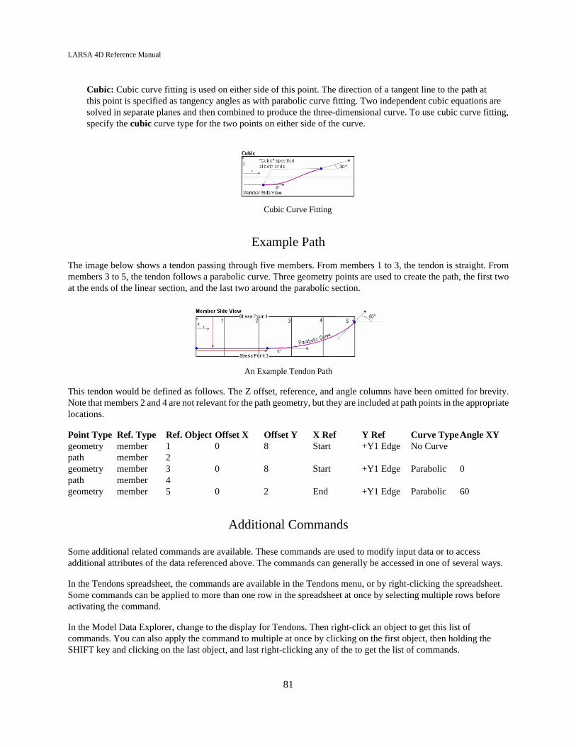
LARSA 4D Reference Manual
Cubic: Cubic curve fitting is used on either side of this point. The direction of a tangent line to the path atthis point is specified as tangency angles as with parabolic curve fitting. Two independent cubic equations aresolved in separate planes and then combined to produce the three-dimensional curve. To use cubic curve fitting,specify the cubic curve type for the two points on either side of the curve.
Cubic Curve Fitting
Example Path
The image below shows a tendon passing through five members. From members 1 to 3, the tendon is straight. Frommembers 3 to 5, the tendon follows a parabolic curve. Three geometry points are used to create the path, the first twoat the ends of the linear section, and the last two around the parabolic section.
An Example Tendon Path
This tendon would be defined as follows. The Z offset, reference, and angle columns have been omitted for brevity.Note that members 2 and 4 are not relevant for the path geometry, but they are included at path points in the appropriatelocations.
Point Type Ref. Type Ref. Object Offset X Offset Y X Ref Y Ref Curve TypeAngle XYgeometry member 1 0 8 Start +Y1 Edge No Curvepath member 2geometry member 3 0 8 Start +Y1 Edge Parabolic 0path member 4geometry member 5 0 2 End +Y1 Edge Parabolic 60
Additional Commands
Some additional related commands are available. These commands are used to modify input data or to accessadditional attributes of the data referenced above. The commands can generally be accessed in one of several ways.
In the Tendons spreadsheet, the commands are available in the Tendons menu, or by right-clicking the spreadsheet.Some commands can be applied to more than one row in the spreadsheet at once by selecting multiple rows beforeactivating the command.
In the Model Data Explorer, change to the display for Tendons. Then right-click an object to get this list ofcommands. You can also apply the command to multiple at once by clicking on the first object, then holding theSHIFT key and clicking on the last object, and last right-clicking any of the to get the list of commands.
81

LARSA 4D Reference Manual
In the graphics window, activate the Pointer mouse tool from the toolbar, and then right-click an object in thegraphical display to get the list of commands to apply to that object.
The additional commands are as follows:
Edit Path and View
This command opens a new spreadsheet window for editing the tendon path and a new graphics window forviewing the path.
Edit Material
This command opens the materials spreadsheet to the material assigned to the tendon.
Duplicate Tendon
This command duplicates the tendon.
Generate Equivalent Loads
This command creates a new load case (page 91) with equivalent member loads based on the forces in thetendon, including anchor set.
Generate Equivalent Loads (before Anchor Set)
This command creates a new load case (page 91) with equivalent member loads based on the forces in thetendon before anchor set is applied.
Compute Jacking Force
Based on the limiting peak stress ratio, proposed jacking force, and short term losses, the applied jacking forceis computed. After changing any values that alter the computation of the applied jacking force, this commandmust be re-run.
The applied jacking force is determined as follows. The limiting force is calculated as the product of the peakstress ratio, material GUTS, strand area, and number of strands. The maximum proposed force is calculated asthe maximum force in the tendon jacked with the proposed jacking force, immediately after anchor set. If themaximum proposed force does not exceed the limiting force, the applied jacking force is set to the proposedjacking force. Otherwise, the applied jacking force is taken as the proposed jacking force multiplied by theratio of the limiting force to the maximum proposed force. This procedure is done twice, first using the interiorpeak stress ratio and the forces all along the tendon, then using the end peak stress ratio and only the force atthe start and end of the tendon. The minimum of the two applied jacking forces found is used.
Mirror Y Offsets
This tool changes all y-offsets in the tendon path to the negative of the offset provided
Mirror Z Offsets
This tool changes all z-offsets in the tendon path to the negative of the offset provided
For More Information, please refer to the following documentation.
• For help on using spreadsheets, see Using the Model Spreadsheets in LARSA 4D User’s Manual.
82

LARSA 4D Reference Manual
Lanes
Lanes define loading paths for vehicles in the moving load analysis (page 179) and for influence-based analysis (page 181).
A lane is a line or surface that travels through a structure. In moving load and influence analysis, the load patternapplied to the structure follows a defined lane path, starting at one end of the path and moving toward the other end.The path of a lane is determined by geometry control points between which straight lines or curves are fit.
Geometry control points are given as offsets relative to members or plates in the model. A lane's geometry points mayreference either all members or all plates. When a lane is defined with reference to members, every member that thelane passes through must be present in the path. Loads will be applied directly to the members listed in the path, withadded moment loads as needed if the lane does not follow the member centroid. If the path references plates, onlyplates containing geometry control points need to be included in the path. Loads will be applied to any plates thatthe path passes through.
For influence surfaces, the lane must be defined with reference to plates, and not members. Only in this case may alane width be specified. For a standard moving load analysis and for influence line analysis when the lane referencemembers, the lane width is ignored for the purposes of the analysis. It may be used by design tools, however.
The type of vehicle to march on the lane is set independently of the lane definition. Use Moving Loads (page 107) toset vehicle parameters.
Basic Properties
These properties are in the Lanes tab of the Geometry Spreadsheets, which is under the Input Data menu. Alternatively,double-click the name of the lane in the lanes section of the Model Data Explorer [in LARSA 4D User’s Manual].
Lane NameA name is assigned by the user to identify the lane.
Lane WidthThe width of the lane where loads can be positioned. This field is used only for influence surface analysis. Notethat for influence surfaces, the lane path must reference only plates and not members, and must have a nonzerowidth.
Skew at Start/EndWhen the lane width is nonzero, skews the start and end of the lane so that the lane is trapezoidal rather thanrectangular. The skew value represents the slope of the edge, with 0 being perpendicular to the direction of thelane and 1 being a 45-degree skew. To compute the skew, find the values of x and y in the figure below. Thevalue of skew-at-start is x/y. In an influence-based live load analysis with UDL patch loading, skew-at-start andskew-at-end must be equal.
83

LARSA 4D Reference Manual
Skew at Start
Path Geometry
Path geometry for a lane is accessed from the lanes spreadsheet above by right-clicking a lane and choosing Edit Path& View. Alternatively, right-click the name of the lane in the lanes section of the Model Data Explorer [in LARSA 4DUser’s Manual] and choose the same command.
Paths consist of a list of geometry control points and path-only points. Geometry points determine the points in spacethat the path follows. A path can contain any number of geometry points, and they are specified with reference tothe member or plate that the point falls within. Geometry points can be offset from member centroids to model laneswith eccentricity.
A path may reference either members or plates, but not both. When a path references members, it must list everymember the path passes through in the right order. Although every member must be listed, there does not need to bea geometry control point in each member. For instance, a straight line lane needs only two geometry points, one atthe start and one at the end, but must list every member that the lane passes through between the geometry points.Include those members with path-only points.
When a path is used to create an influence surface, bear in mind that the geometry of the surface (a rectangle in 3Dspace) is distinct from the set of plates to which influence surface unit loading will be applied. It is typically notnecessary to list all of the plate elements to which influence surface loading will be applied in the path spreadsheet.When the surface geometry intersects with the physical dimensions of every plate, LARSA 4D will automaticallydetermine which plates to load. However, if the surface is elevated above the plate elements, or if the plate elementshave a cross-slope such that the surface geometry does not intersect with the physical dimensions of plate elements,then plate elements that do not intersect the surface geometry must be listed in the path spreadsheet as path-only points.These points can be listed anywhere on the path, including at the end.
The following describes the data used to define each point in a path.
Point TypeNot every member that a lane passes through will need a geometry point, but each member passed throughmust be specified in the path, in the order in which the lane passes through them. For those members the lanepasses through but in which no geometry control point is needed, use the path only point type. Otherwise, usethe geometry point type.
The span break point type is a marker indicating that the lane has crossed into another span on a bridge, fordesign purposes. This does not affect the computation of the influence coefficients, but the location of span breaksare used in influence-based results (page 181) for compliance with the AASHTO LFD and BS5400 codes. Thespan break marker indicates that the previous geometry point gives the coordinates of the end of a span; thus,span break markers should immediately follow a geometry point positioned over a support.
Reference Object Type
84

LARSA 4D Reference Manual
Select whether this point references a member or plate.
Reference Object or Range
• For geometry points, specify the ID of the member or plate that this point is within. The offset coordinate forthis point is specified in the local coordinate system of this member or plate. Specify a range of IDs, such as12-36, or even 36-12, to repeat this point for each member or plate in the range, in the order specified.
• For path only points, specify an ID or range of IDs for the members that this point is acting as a placeholderfor.
The remaining fields are for geometry point only.
Offset (X, Y and Z)For geometry points, the offset of this point from some position within the referenced object. Offset directionsare in the element's reference axis directions, rather that in global axis directions. The offset is by defaultrelative to the start of the member or the I-joint of the plate. Y- and z-offsets in lanes on members will createmoments. For influence surfaces, a z-offset will create a moment if the load direction is either Local X or LocalY.
Reference (X, Y and Z)
For points referencing members, set the X Reference to End to position the point relative to the end of the member.Positive values for X Offset are then toward the beginning of the member.
The y and z reference fields are not normally changed from Reference Line so that the y and z offset fields arein the member reference axes. See the documentation for tendon paths (page 75) for more on the other choices forthe y and z reference fields.
By default, geometry points on members will fall at the start of the member on its reference line, which normally is atits centroid (except see section centroid offsets (page 21)). Loading at this position will be applied directly to the memberwithout any eccentricity. To apply eccentricity, use the offset fields described above.
Points that reference plates by default will fall at the I-joint of the plate. Use the X and Y offsets, which are in theplate's local coordinate system, to position the geometry point.
The geometry points on the path will by default be connected by straight lines, meeting at hard corners if the laneturns. For descriptions of the curve fitting options, see the documentation for tendon paths (page 75).
Lane Path Example
A straight lane that passes through members 1 through 10 should be defined as follows:
Point Type Ref. Type Ref. Objector Range
Offset X Offset Y Offset Z X Ref Y Ref Z Ref
geometry member 1 0 0 0 Start ReferenceLine
ReferenceLine
path member 2-9geometry member 10 0 0 0 End Reference
LineReferenceLine
Note that the last point has its X Reference set to End so that the lane goes through all of member 10, rather thanstopping at its start joint.
85
LARSA 4D Reference Manual
If members 1 through 10 are on a curve, the lane above will not follow the curve. It will only be a straight line betweenthe two geometry points defined. To have the lane follow the curve, there should be a geometry point at the start andend of every member. Without these geometry points, the lane will not exactly following the centroids of the members,leading to inadvertent eccentricities. That lane is defined as follows:
Point Type Ref. Type Ref. Objector Range
Offset X Offset Y Offset Z X Ref Y Ref Z Ref
geometry member 1 0 0 0 Start ReferenceLine
ReferenceLine
geometry member 2 0 0 0 Start ReferenceLine
ReferenceLine
geometry member 3 0 0 0 Start ReferenceLine
ReferenceLine
...geometry member 10 0 0 0 Start Reference
LineReferenceLine
geometry member 10 0 0 0 End ReferenceLine
ReferenceLine
Note that member 10 is referenced twice so that a point is placed at its start and end. This can be abbreviated as:
Point Type Ref. Type Ref. Objector Range
Offset X Offset Y Offset Z X Ref Y Ref Z Ref
geometry member 1-10 0 0 0 Start ReferenceLine
ReferenceLine
geometry member 10 0 0 0 End ReferenceLine
ReferenceLine
Additional Commands
Some additional related commands are available. These commands are used to modify input data or to accessadditional attributes of the data referenced above. The commands can generally be accessed in one of several ways.
In the Lanes spreadsheet, the commands are available in the Lanes menu, or by right-clicking the spreadsheet.Some commands can be applied to more than one row in the spreadsheet at once by selecting multiple rows beforeactivating the command.
In the Model Data Explorer, change to the display for Lanes. Then right-click an object to get this list of commands.You can also apply the command to multiple at once by clicking on the first object, then holding the SHIFT key andclicking on the last object, and last right-clicking any of the to get the list of commands.
In the graphics window, activate the Pointer mouse tool from the toolbar, and then right-click an object in thegraphical display to get the list of commands to apply to that object.
The additional commands are as follows:
Edit Path and View
This command opens a new spreadsheet window for editing the lane path and a new graphics window forviewing the path.
Transfer to Plates
86

LARSA 4D Reference Manual
This command duplicates the lane and modifies all member-based geometry points in the path that fallwithin a plate element to reference the plate element instead. The offset fields are updated appropriately.
For More Information, please refer to the following documentation.
• For help on using spreadsheets, see Using the Model Spreadsheets in LARSA 4D User’s Manual.
• Moving Load Analysis on page 179.
87

LARSA 4D Reference Manual
88

LARSA 4D Reference Manual
Loads
Structure loading is defined in load cases. There are several types of load cases, the most commonly used of which isthe static load case. In static load cases, joint, member, plate, thermal, and other types of static loads can be applied tothe structure. The other load case types include moving load cases, time history cases, and response spectra cases.
The type of analysis chosen determines how load cases are used. Static analyses (Linear Static Analysis (page 137),P-Delta Analysis (page 139), and Nonlinear Static Analysis (page 141)) require static load cases and load combinationsof static load cases. Eigenvalue analyses (page 157) do not make use of load cases at all. The moving load analyses(Moving Load Analysis (page 179) and Influence Line & Surface Analysis (page 181)) require moving load cases withmoving loads. The time history analyses (page 169) require a time history load case with time history excitation loadsand, for some models, initial conditions.
The Response Spectra Analysis (page 159) can be performed with or without static load cases, but it requires a responsespectra case with setup information.
In Staged Construction Analysis (page 205), static load cases are used to define the patterns of loading that will be appliedon the structure at points throughout construction, but they are not applied to the structure until they are assigned toconstruction stages.
Static Load Cases 91Load Classes for Code-Based Results 91
Load Combinations 93Including Response Spectra Cases 93
Including Moving Load Cases 93
Use in Nonlinear Analysis 93
Self Weight 95Weight Factor and Gravity Load Directions 95
Self Weight Computation 95
In Staged Construction Analysis 95
Joint Loads 97
Support Displacements 99
Member Loads 101
Member Thermal Loads 103Load Input 103
Nonlinear Thermal Gradient Curves 104
Plate Loads 105Plate Load Fields 105
Point Load Coordinates 106
89

LARSA 4D Reference Manual
Moving Loads 107
Influence Loads 109
Time History Loads 111Excitation Functions 111
Initial Conditions 112
90

LARSA 4D Reference Manual
Static Load Cases
A static load case represents one scenario of static loading.
The following loads may be applied in static load cases.
• Self Weight (page 95) for automatic computation of gravitational loading based on section and materialproperties of elements.
• Joint Loads (page 97): Forces and moments applied at joints
• Support Displacements (page 99)
• Member Loads (page 101) on beams (point loads, uniformly or partially distributed loads, and triangularloads), including pre- and post-tensioning of members such as cables
• Member Thermal Loads (page 103): Uniform thermal loads for beam, truss, and cable elements, and thermalgradients for beam elements
• Plate Loads (page 105): Concentrated and uniform loads applied on plate and shell elements
• Thermal Plate Loads (page 105): Temperature change through the thickness of plate and shell elementsresulting in uniform and thermal gradients
Load cases can be marked Inactive. Inactive load cases are excluded from analysis runs.
Load cases also have the option "Is Dynamic Mass?" This option affects the dynamic analysis types only, includingeigenvalue, RSA, and time history. When this option is Yes, the loads in this case are treated as representing mass.All load cases with the option set to Yes are included as dynamic mass, in addition to any other mass specified in themodel, in all dynamc analysis types.
Load Classes for Code-Based Results
Load cases can be assigned a load class, such as dead load, rain, and vehicular live load. These classes have beengathered from various codes and are used to pick out class-based results and to automate the process of creating class-based load combinations. Load classes can be chosen from the Load Cases Explorer [in LARSA 4D User’s Manual].
To create code-based load combinations, the Automatic Code-Based Load Combinations [in LARSA 4D User’sManual] tool is useful. Class-based cumulative results can be obtained in the results spreadsheets [see “ResultsSpreadsheets” in LARSA 4D User’s Manual] in staged construction analysis.
For More Information, please refer to the following documentation.
• For help creating and editing load cases, see Load Cases Explorer in LARSA 4D User’s Manual.
• For help on using spreadsheets, see Using the Model Spreadsheets in LARSA 4D User’s Manual.
• Analysis Reference on page 131.
91

LARSA 4D Reference Manual
92

LARSA 4D Reference Manual
Load Combinations
Load combinations represent the combined application of load cases. They are defined before an analysis is run.
In a linear analysis, load combinations are computed by linearly combining the results of the static cases. However,in the nonlinear anlysis types, load combinations are computed by analyzing the load combination's load casesconsecutively, carrying the effect from each case into the next.
Load combinations are most often used for combining static load cases with other static load cases and combiningstatic cases with seismic cases. They can also combine static cases with moving load cases, but the behavior of loadcombinations varies slightly when non-static load cases are included. Use Linear Result Combinations [in LARSA 4DUser’s Manual] to combine the results of a Time History Analysis with other results.
Load combinations can be analyzed in static, moving load, and response spectra analyses.
Each load case in a combination can be assigned a Load Factor which determines its contribution to the combination.
Load combinations are primarily needed for codes, to check or design the structure under various loading conditions.Linear Result Combinations [in LARSA 4D User’s Manual] can also be used to combine results. Automatic Code-BasedLoad Combinations [in LARSA 4D User’s Manual] can be used to automatically create code-based combinations.
Including Response Spectra Cases
Response Spectra Analysis (page 159) results generally do not have a sign convention. When an RSA case is includedin any combination, its contribution is included with positive sign multiplied by the load factor.
To account for both the positive and negative directions of an earthquake, create two load combinations using the RSAcase, one with a positive load factor for the RSA case and the other with a negative load factor.
Including Moving Load Cases
Up to two Moving Load Analysis (page 179) cases can be included in a Load Combination. If one moving load case isincluded in a combination, then LARSA creates a group of result cases, one for each generated case for the moving loadcase, each combining the effects of the static loads in the combination and the corresponding moving load result case.
If two moving load cases are included in a combination, then LARSA generates a group of generated load cases, onefor each combination of a generated case from the first moving load case and a generated case from the second movingload case. If there are 1,000 generated cases in the first group and 1,000 in the second group, then one million caseswill be generated. Because the number of generated load cases can quickly grow out of hand, using the Influence Line& Surface Analysis (page 181) is recommended instead.
Use in Nonlinear Analysis
In a nonlinear static analysis, load combinations are treated differently than in a linear static analysis, and their behaviorcan vary between analysis types.
93

LARSA 4D Reference Manual
Nonlinear Static Analysis (page 141)
Load cases within a Load Combination represent increments. The analysis is performed for each case inthe combination as the load vector of the case multiplied by the corresponding load factor. The results ofeach increment are not saved and cannot be viewed later. Only the results after all cases have been appliedare reported.
Nonlinear Buckling (page 145) and Restart AnalysisLoad combinations themselves are treated as incremental load steps. Results are accumulated from one loadcombination to the next. Only static load cases can be included in the combinations.
For More Information, please refer to the following documentation.
• For help on using spreadsheets, see Using the Model Spreadsheets in LARSA 4D User’s Manual.
• For help on using the Load Cases Explorer, see Load Cases Explorer in LARSA 4D User’s Manual.
• Linear Result Combinations in LARSA 4D User’s Manual.
94
LARSA 4D Reference Manual
Self Weight
The automatic computation of self-weight (gravity loading) can be included in static load cases (page 91) by specifying aweight factor in the direction of gravity. The weight factor for X, Y and Z are specified with the load case descriptiondata.
Weight Factor and Gravity Load Directions
The gravity load directions are the directions of the Global Coordinate System. A positive factor implies that self-weight is acting in the positive direction of the axes. A negative factor implies that self-weight is acting in the negativedirection.
The user may choose to apply the gravity loading in one direction at a time or in any combination of X, Y and Zdirections.
A value of -1.00 for Weight Factor Z would instruct the program to apply 100 percent of the computed self weight ofthe structure in the negative Z-axis direction, which properly simulates gravity for a structure where the Z-axis is up.A value of 1.00 for Weight Factor X and 0.50 for Weight Factor Y would instruct the program to apply 100 percentof the computed self weight in the direction of X-axis and 50 percent in the direction of Y-axis simultaneously.
The self weight factors are used in static analyses only. For dynamic analysis, the mass due to the weight of an elementis computed and applied automatically in all translational directions X, Y and Z when the weight density of the materialis specified as nonzero. See also Mass elements (page 71). You can create additional mass with the dynamic mass optionon static load cases (page 91).
Self Weight Computation
The weight of members (page 49) are computed using the cross sectional area, element length and weight density. Theweight of plates (page 61) are computed using the element volume and the weight density.
The self-weight of beam elements are modeled using uniformly distributed loads. This approach generates a consistentload vector considering the bending and shear effects due to the self-weight. The program computes the equivalentuniform load using the gravitational factors, direction, section area and weight density. Nonprismatic members use theaverage of the cross-sectional area at the member ends.
For plates, self-weight is computed based on material weight and thickness. Uniform pressure loads are used.
Springs, isolators, and tendons do not contribute to the weight of the model.
In Staged Construction Analysis
In a Staged Construction Analysis (page 205), self-weight loading must be applied to include the self-weight of elementsin the analysis. Place a load case with self-weight turned on in every step in which new elements are constructed ifself-weight is desired for those elements.
95

LARSA 4D Reference Manual
Self-weight load cases only apply self-weight to elements constructed in the same construction step as the self-weightload case. Therefore you must place a self-weight load case in the same construction step in which elements areconstructed.
If a self-weight load case is placed in a construction step without a construction activity, self-weight loading will beapplied (possibly again) to all elements in the model constructed up to that point.
To omit self-weight for elements in Staged Construction Analysis, there are two options. You may omit the self-weight load case in the construction step in which the elements are constructed. Alternatively, you may construct theelements with the stiffness-only option. In the Construction Stages Explorer [in LARSA 4D User’s Manual] right-clickthe structure group of elements and choose Stiffness Only. With this option, self-weight will be skipped even if a self-weight load case is present.
When a dynamic analysis is performed as an analysis scenario (page 129) in Staged Construction Analysis, element massis computed automatically for elements constructed normally. Elements constructed with the stiffness-only option willnot have mass. (If an element is constructed normally, that is with stiffness and weight, but a self-weight load caseis not applied, mass will still be included.)
For More Information, please refer to the following documentation.
• For help on using spreadsheets, see Using the Model Spreadsheets in LARSA 4D User’s Manual.
96

LARSA 4D Reference Manual
Joint Loads
Joint loads can be applied at the joints of the structure. The applied forces are specified in the displacement coordinatesystem of the joint, which is by default the Global Coordinate System.
Multiple joint loads can be applied to the same joint in a load case.
Joint loads are static loads and are applied in static load cases (page 91).
JointThe ID of the joint to which this joint load will be applied.
Force X/Y/ZThe applied translational force in the joint's displacement coordinate system.
Moment X/Y/ZThe applied moment in the joint's displacement coordinate system.
If the joint is assigned a cylindrical coordinate system, the X, Y, and Z components of the load correspond to the R,Theta, and Z axes of the UCS. Specifying an x-component results in a load directed radially from the center of theUCS, with positive loads directed away from the origin. Specifying a y-component results in a tangentially-directedload, with positive loads directed counter-clockwise about the origin.
If the joint is assigned a spherical coordinate system, the X, Y, and Z components of the load correspond to the R, Phi,and Theta axes of the UCS. Specifying an x-component results in a load directed radially from the center of the UCS,with positive loads directed away from the origin. Specifying a y- or z-component results in a tangentially-directedload in the phi and theta directions, respectively.
For More Information, please refer to the following documentation.
• For help on using spreadsheets, see Using the Model Spreadsheets in LARSA 4D User’s Manual.
• Joints on page 47.
97

LARSA 4D Reference Manual
98
LARSA 4D Reference Manual
Support Displacements
Support displacement loads can be applied at the joints of the structure. The applied displacements are specified in thedisplacement coordinate system of the joint, which is by default the Global Coordinate System.
Support displacement loads can only be applied to joints in degrees of freedom that are fixed at the joint. If a supportdisplacement load in any load case is applied to a joint in a direction in which the joint is not restrained, the joint willbecome restrained in that direction in all load cases in the project.
Support displacement loads are static loads and are applied in static load cases (page 91). A joint can have only onesupport displacement in a load case.
Support displacements are also referred to as support settlements and joint displacement loads.
JointThe ID of the joint to which this joint load will be applied.
Translation X/Y/ZThe translational displacement in the joint's displacement coordinate system.
Rotation X/Y/ZThe rotational displacement in the joint's displacement coordinate system.
For More Information, please refer to the following documentation.
• For help on using spreadsheets, see Using the Model Spreadsheets in LARSA 4D User’s Manual.
99

LARSA 4D Reference Manual
100

LARSA 4D Reference Manual
Member Loads
Member loads encompass a wide range of loads that can be applied to members, including concentrated forces andmoments and distributed forces and moments.
Member loads can be specified in the local coordinate directions of the member or in the Global Coordinate System.Distributed loads can also be specified as projected loads in the Global Coordinate System directions.
These loads are positive when acting on the member in the positive direction of the specified reference axis. The loadsare always assumed to act on the centroid axis of the member.
Because truss and cable elements have only axial stiffness, laterally applied loads are transferred to the joints themember is connected to, unlike in beam elements for which the fixed-end-force concept is used.
Multiple member loads may be applied to the same member in a load case.
MemberThe ID of the member to which the load will be applied.
TypeThe type of the load.
• Point Force/Point Moment - A force or moment applied at a single point on the member.
• Uniform Force/Moment - A uniform force or moment applied along a part or all of the length of themember.
• Trapezoidal Force/Moment - A force or moment applied along a part of the length of the member withvarying magnitude at the beginning and at the end of the applied load.
• Pre-Tension - This load type is usually used for cable elements in shape finding or for construction analysisof cable structures. The pre-tension load is the initial cable force at the beginning of the analysis step, but thecable force may be reduced or increased due to applied loads or other structural changes as they are applied.
• Post-Tension - This load type is usually used for cable elements in shape finding or for construction analysisof cable structures. The post-tension load will force the rest of the structure to adjust in order to keep thecable force constant at the specified magnitude, simulating the jacking operation at a constant force on acable.
• Jacking Elongation - Simulates the jacking operation in cable tensioning. The jacking elongation loadspecifies the change in the length of the member, which is used only in nonlinear analyses.
The pre- and post-tension load types are only used in a nonlinear analysis, both static and Staged Construction Analysis.
DirectionLoads can be applied in the local or the global coordinate system. Positive magnitude loads are in the directionof the positive axis selected. Specify negative magnitudes to apply the load in the negative axis direction.
Local X/Y/Z. The load acts in the direction of the local axis of the member.
Global X/Y/Z. The load acts in the direction of the global axis.
Projection on Global X/Y/Z. Applies to uniform or partially distributed loads. The direction of the load is in thedirection of the global axis, and the magnitude of the load is measured per projected length. The projected lengthis in the plane perpendicular to the direction of loading.
101

LARSA 4D Reference Manual
The direction is not applicable for pre/post-tension loads or jacking elongation, which are applied axially.
Magnitude at StartFor point and uniform loads, the magnitude of the load. For trapezoidal loads, the magnitude at the beginningof the load application.
Magnitude at EndFor trapezoidal loads, the magnitude at the end of the load application. Not applicable for other load types.
Start PositionFor point loads and pre-/post-tension loads, the location of the load. For distributed loads, the location of thestart of the load application. Specified relative to the member length (e.g. 0.0 is the start of the member at the I-Joint and 1.0 is the end of the member at the J-Joint), or in absolute length units, measured along the length ofthe member. If the member has an end offset, the position is not measured from the joints but instead from theoffsetted end positions.
End PositionFor distributed loads, the location of the end of the load application, specified in the same way as the StartPosition, relative to the start of the member. Not applicable for other load types.
ShorteningThe shortening length. Only applicable for Jacking Elongation loads.
Additional Commands
Some additional related commands are available. These commands are used to modify input data or to accessadditional attributes of the data referenced above. The commands can generally be accessed in one of several ways.
In the Member Loads spreadsheet, the commands are available in the Member Loads menu, or by right-clicking thespreadsheet. Some commands can be applied to more than one row in the spreadsheet at once by selecting multiplerows before activating the command.
The additional commands are as follows:
Enter Absolute Positions
Choosing this option sets the start and end position fields to use absolute length units. 0.0 represents the startof the member, and the length of the member is used to give the position at the end of the member.
Enter Relative Positions
Choosing this option sets the start and end position fields to use relative units. 0.0 represents the start of themember, and 1.0 represents the end of the member.
For More Information, please refer to the following documentation.
• Members on page 49.
• For help on using spreadsheets, see Using the Model Spreadsheets in LARSA 4D User’s Manual.
102

LARSA 4D Reference Manual
Member Thermal Loads
The loading due to temperature change in a member can be specified using Member Thermal Loads.
With uniform thermal loading, a constant temperature change is applied to the entire member cross-section. Uniformthermal loading normally produces axial strain only. Linear and nonlinear thermal gradients create a temperaturechange that is uniform along the length of the member but that varies either from section top to bottom or from sectionleft to section right. All thermal loads are constant along the length of the member.
When applied to composite sections starting in LARSA 4D 7.9, thermal loading will use the material assigned to eachshape in the section if a material is assigned to section shapes. If either the material modulus of elasticity or coefficientof thermal expansion differ between shapes in the section, rotational strain may result and self-equilibriating stresses(also known as eigenstresses) will be accumulated and included in member stress results (page 247). Prior to LARSA4D 7.9, the material assigned to the member was assumed constant throughout the cross-section (and, therefore, noself-equilibriating stresses were possible).
Nonlinear gradients are available starting in LARSA 4D 7.9. The resulting self-equilibriating stresses will beaccumulated and included in member stress results (page 247).
The coefficient of thermal expansion specified in the material data of the element (or shapes) must have a nonzerovalue, otherwise there will be no thermal effects for the element. Only uniform thermal loads should be applied totruss and cable elements.
Multiple member thermal loads can be applied to a member in a load case.
Load Input
MemberThe ID of the member to which the load will be applied.
TypeThe type of the load: Uniform, Linear, or Nonlinear.
Variation DirectionFor linear or nonlinear gradient thermal loading, specifies whether the variation changes along the local-y orlocal-z axis of the member.
Temperature Change at TopFor uniform loads, specifies the change in temperature. For linearly varying loads, specifies the temperaturechange at the top edge (+y) or right edge (+z) of the member. In LARSA 4D through version 7.7, the locationof the top or right is determined by the location of the first section stress recovery point (page 21), which isassumed to be at an extreme fiber. Starting in LARSA 4D 7.9, the section geometry from the Section Composeror the section dimensions (page 21) spreadsheet is used to compute the section extents (and the stress recoverypoints are ignored). Top and right refer to the location of the fiber at the highest y or z coordinate.
Temperature Change at BottomFor linearly varying loads, specifies the temperature change at the bottom edge (-y) or left edge (-z) ofthe member. Not applicable for uniform loads. The location of the bottom and left edge follows a similarconvention for the top and right edges. In LARSA 4D through version 7.7, the third section stress recovery
103

LARSA 4D Reference Manual
point is assumed to be at an extreme -y/-z fiber. Starting in LARSA 4D 7.9, the section geometry is usedinstead.
Nonlinear Temperature CurveSpecifies the nonlinear temperature curve to apply. Create a curve in the Input Data # Properties #Temperature Curve spreadsheet first.
Nonlinear Thermal Gradient Curves
Nonlinear thermal gradient curves are entered in a spreadsheet located at Input Data # Properties # TemperatureCurve . Add a row to this spreadsheet and name the curve. Then right-click the spreadsheet and choose Edit Curve .
Add rows to this spreadsheet to specify location and temperature change values on the curve.
Temperature ChangeEach temperature value is specified in load-temperature units (see Model Units [in LARSA 4D User’sManual]). It is the temperature change at a location in the cross-section.
Location ReferenceThe location of each temperature coordinate is specified in one of four ways: + Edge indicates the locationis measured from the extreme +y or +z fiber (depending on the Variation Direction specified in the loadspreadsheet). - Edge indicates the location is measured from the extreme -y or -z fiber. In both cases positivevalues are toward the centroid. Rel. indicates that the location is specified relative to the member depth orwidth in the range from 0.0 to 1.0. Abs. indicates the location is specified in section length units. For instance,using the + Edge, Rel. option, the value 0.0 indicates the top or right edge of the section and 0.25 specifies alocation 1/4th the way into the section from the top or right. Or, using the - Edge, Abs. option, the value 0.0indicates the bottom or left edge of the section and 5.8 specifies a location 5.8 section units into the sectionmeasured from the left or bottom.
For More Information, please refer to the following documentation.
• Members on page 49.
• For help on using spreadsheets, see Using the Model Spreadsheets in LARSA 4D User’s Manual.
104

LARSA 4D Reference Manual
Plate Loads
Uniformly distributed pressure loads, concentrated forces, and thermal loads can be applied to plates.
Uniformly distributed loads can be specified in the local coordinate directions of the plate or in the Global CoordinateSystem directions, or as projected loads in the Global Coordinate System directions. Point loads can be specified inthe local coordinate directions of the plate or in the Global Coordinate System directions.
Temperature loads on plates can be specified as a uniform change or as a linear temperature gradient through thethickness of the element. The temperature effects are assumed to be constant over the lateral directions of the element.The coefficient of thermal expansion specified in the material data of the element must have a nonzero value, otherwisethere will be no thermal effects.
Temperature increase is positive for uniform temperature change. Uniform temperature loading causes in-plane(lateral) expansion. Temperature gradient loading causes out-of-plane bending only.
Multiple plate loads can be applied to a plate in a load case.
Plate Load Fields
PlateThe ID of the plate to which the load will be applied.
TypeDetermines the type of the load.
• Point Force - A force applied at a single point on the element.
• Uniform Force - A uniform force applied on the surface of the element.
DirectionLoads can be applied in the local or the Global Coordinate System. Positive magnitude loads are in thedirection of the positive axis selected.
Local X/Y/Z. The load acts in the direction of the local axis of the plate.
Global X/Y/Z. The load acts in the direction of the global axis.
Projection on Global X/Y/Z. Applies to uniform loads. The direction of the load is in the direction of the globalaxis, and the magnitude of the load is measured per projected area. The projected area is in the plane perpendicularto the direction of loading.
MagnitudeThe magnitude of the load. For uniform loads, the load is constant throughout the plate.
Relative X Location (x/XL)For point loads, the relative distance of the load with respect to the I-J or K-L sides of the element, as explainedbelow.
Relative Y Location (x/XL)
105

LARSA 4D Reference Manual
For point loads, the relative distance of the load with respect to the J-K side of the element for quadrilateralplates and with respect to the local y-axis for triangular plates, as explained below.
Uniform TemperatureThe uniform temperature change. Positive values are an increase in temperature by that many degrees.
Temperature GradientThe temperature change per unit of length measured perpendicular to the plate, i.e. through the thickness of theelement. Positive values mean the top (+z side) is subject to a temperature increase while the bottom (-z side)is subject to a temperature decrease. The middle of the plate (z=0) has no temperature change. For example,if a plate 3 inches thick is given a 4 degrees/foot temperature gradient, it experiences a 1-degree temperatureincrease on its top surface, no temperature change at z=0, and a -1 degree temperature change at its bottomsurface.
Point Load Coordinates
The locations of point force loads on plates are specified in a special coordinate system which is neither the globalnor plate local coordinates. The choice of coordinate system is intended to simplify the specification of the locationso that the x- and y-coordinates are both in the range [0, 1].
For quadrilateral plates, the load coordinates of the four corners of the plate from I to L are (0,0), (1,0), (1,1), (0,1).For rectangular plates, the load coordinates are simply scaled plate local coordinates. For irregularly shaped plates, theload coordinates are essentially warped to fit in the quadrilateral shape. See the following figure:
Load coordinate specification for quadrilateral plates
(I-, J-, K-, and L-joints refer to the first, second, third, and fourth joints, respectively, that define the plate geometryin the plates spreadsheet (page 61).)
The load location specification for triangular plates is on a scaled local coordinate system, as with perfectly rectangularplates. The load coordinates of the three corners of the plate from I to K are (0,0), (1,0), and (q,1), for some q. Fortriangular plates, unlike quadrilateral plates, not every coordinate with components in the range [0, 1] will actually fallwithin the plate area. The coordinate grid for load specification on triangular plates is shown below:
Load coordinate specification for triangular plates
For More Information, please refer to the following documentation.
• Plates on page 61.
• For help on using spreadsheets, see Using the Model Spreadsheets in LARSA 4D User’s Manual.
106

LARSA 4D Reference Manual
Moving Loads
Moving loads are added into moving load cases for the Moving Load Analysis (page 179). These loads specify how togenerate the result cases for a vehicle moving on a user-defined path (lane) on a structure.
The analysis requires a database file containing the load patterns [see “Connecting Databases” in LARSA 4D User’sManual], geometry definition of lanes (page 83), and load cases in which the user can specify the load pattern, the loadedlane and related data for a traveling load pattern.
A single load case with multiple moving loads simulates the simultaneous marching of the loads. Multiple load casescan be used to simulate multiple independent vehicles on the same lane or multiple lanes.
Moving load cases can be combined with static load cases, response spectra cases, and with other moving load cases.Combinations can be made within the analysis using Load Combinations (page 93) or after the analysis using LinearResult Combinations [in LARSA 4D User’s Manual].
Lane LoadedThe lane (page 83) on which the load pattern will be marching.
Load PatternThe load pattern to march on the lane. All load patterns from connected moving load pattern databases areavailable to choose from. See Connecting Databases [in LARSA 4D User’s Manual].
Applied Load DirectionThe direction of the load application. The direction can be in the local coordinate systems of the members thelane passes through, or in global directions. Positive magnitude loads are in the direction of the positive axisselected.
Load FactorA factor to scale the load pattern. The default is 1.0.
Direction of TravelThe load pattern can march forward on the lane, backward, or both, meaning first forward then backward.
Position IncrementThe distance between each successive position of the load pattern as it marches along the lane. Smallerincrements will generate more result cases but may be more informative and accurate.
Start PositionThe starting position of the load, measured in length units along the lane from the start of the lane. 0.0 is thestart of the lane.
For More Information, please refer to the following documentation.
• For help on using spreadsheets, see Using the Model Spreadsheets in LARSA 4D User’s Manual.
• Lanes on page 83.
• Standard Vehicles on page 199.
• Moving Load Analysis on page 179.
• Connecting Databases in LARSA 4D User’s Manual.
107

LARSA 4D Reference Manual
• Influence Loads on page 109.
108

LARSA 4D Reference Manual
Influence Loads
Influence loads are added into moving load cases for the Influence Line & Surface Analysis (page 181). These loadsspecify how to generate the result cases for a unit load moving on a user-defined path or surface.
The analysis requires the geometry definition of lanes (page 83) and load cases in which the the loaded lane and relateddata for a traveling load pattern are specified.
A separate moving load case is required for each lane to be considered. In each load case, a single influence load isapplied to that lane. In some circumstance, it may be appropriate to apply two or more influence loads into a singlemoving load case to simulate the distribution of vehicle axle loads onto multiple girders. In these cases, the factorsshould sum to 1.0 and the lanes must all be of the same length.
Lane LoadedThe lane (page 83) on which the unit load will be marching. If the lane is defined with reference to members, it isa linear path for an influence line. If the lane is defined with reference to plates, it is a surface for an influencesurface analysis and width should be specified for the lane.
Applied Load DirectionThe direction of the load application. The direction can be in the local coordinate systems of the membersor plates the lane passes through or in global directions. Local directions are recommended. When the laneincludes offsets from the member centroid (such as for live load centrifugal and braking forces conditions),local directions must be used. Moments due to the offset will not be created when the applied load direction isin a global direction. Positive magnitude loads are in the direction of the positive axis selected.
Load FactorA factor to scale the unit load. The default is 1.0.
Forward IncrementThe distance between each successive position of the load pattern as it marches along the lane.
Transverse IncrementUsed for influence surfaces only. The transverse distance between lateral strips used to approximate thesurface. The transverse increment must divide the lane width evenly; if it does not, LARSA will round-upthe increment. A transverse increment of zero instructs LARSA to choose a sensible increment based on theforward increment.
Smaller increments will generate more result cases but may be more informative and accurate.
For More Information, please refer to the following documentation.
• For help on using spreadsheets, see Using the Model Spreadsheets in LARSA 4D User’s Manual.
• Lanes on page 83.
• Standard Vehicles on page 199.
• Moving Load Analysis on page 179.
• Influence Line & Surface Analysis on page 181.
109

LARSA 4D Reference Manual
110

LARSA 4D Reference Manual
Time History Loads
Time history loads include Applied Excitation Functions and Initial Conditions. They are applied in time history loadcases for the Linear Time History Analysis (page 169) and Nonlinear Time History Analysis (page 171).
Excitation Functions
Time-based excitation functions are applied at joints in any of the six directions of motion. There are two types ofexcitation functions.
Uniform base excitations, which must be force or acceleration functions, are applied to all free joints in the model.
Joint-localized excitations are applied at one or more specified joints. Multiple excitation functions can besimultaneously applied in more than one direction at the same joint, or at more than one joint. Displacement excitationfunctions can be applied only to joints with fixed DOF in the direction of the excitation function, while force andacceleration excitation functions can be applied only at joints free to move in the direction of the excitation function.
Before entering the load data for a time history case, the database file containing the time history curves must beconnected to the project. See Connecting Databases [in LARSA 4D User’s Manual].
The data required for excitations is below:
JointThe ID of the joint to which the excitation will be applied. For uniform base excitation, leave blank.
Time History CurveThe time history records curve to be applied at this joint, selected from all of the time history curves indatabases connected to the project.
Displacement FunctionMay only be applied at joints restrained in the direction of the excitation, which are usually supports.Displacement functions are not applicable as a uniform base excitation.
Force FunctionsAs a joint-localized excitation, this type of function may only be applied at joints free in the direction ofthe excitation. As a uniform base excitation, the force is applied to all such joints.
Acceleration FunctionsAs a joint-localized excitation, this type of function may only be applied at joints free in the direction ofthe excitation. As a uniform base excitation, the force is applied to all such joints. An equivalent force isapplied at the joint computed as acceleration multiplied by the mass at the joint. The mass is the sum ofthe mass due to elements connected to the joint (computed in the same way as self-weight (page 95)), massspecified on a mass element (page 71) at the joint (in the applied direction of the excitation function), andequivalent mass specified in load cases (page 91) with the Is Dynamic Mass option turned on.
A single time history case must have either displacement or force/acceleration curve types.
Applied DirectionThis is the direction of the applied load. The excitation function is applied in the joint's displacement coordinatesystem, which is by default the Global Coordinate System.
111

LARSA 4D Reference Manual
• Translation X/Y/Z - Indicates the direction of the translational excitation function, for force, displacement,or acceleration curves.
• Rotation X/Y/Z - Indicates the direction of the rotational excitation function, for force, displacement, oracceleration curves.
Initial Conditions
Initial conditions are for initial nonzero displacements, velocities, and accelerations. When no initial conditions arespecified, the structure is assumed at rest initially.
The following data is used for initial conditions:
JointThe ID of the joint for which this initial condition applies.
DisplacementThe initial displacement of the joint.
VelocityThe initial velocity of the joint.
AccelarationThe initial acceleration of the joint.
DirectionThe direction of the specified displacement, velocity, and acceleration. May be translational or rotational in x,y, or z. The directions are in the joint's displacement coordinate system.
Additional Commands
Some additional related commands are available. These commands are used to modify input data or to accessadditional attributes of the data referenced above. The commands can generally be accessed in one of several ways.
In the Time History Excitations spreadsheet, the commands are available in the Time History Excitations menu, orby right-clicking the spreadsheet. Some commands can be applied to more than one row in the spreadsheet at onceby selecting multiple rows before activating the command.
The additional commands are as follows:
Add Excitation for Selected Joints
This command adds excitation records to the active load case for every selected joint.
For More Information, please refer to the following documentation.
• For help on using spreadsheets, see Using the Model Spreadsheets in LARSA 4D User’s Manual.
• Linear Time History Analysis on page 169.
• Nonlinear Time History Analysis on page 171.
• Connecting Databases in LARSA 4D User’s Manual.
112
LARSA 4D Reference Manual
Construction Activities
In the Staged Construction Analysis, changes to the structure are modeled as construction activities. Data input forconstruction activities is described in this section.
Construction activities are used in the Staged Construction Analysis (page 205) and are added in the Construction StagesExplorer [in LARSA 4D User’s Manual], or with the Construction Stage Editor [see “Construction Stage Editor” inLARSA 4D User’s Manual] in the Input Data menu.
For More Information, please refer to the following documentation.
• Staged Construction Analysis on page 205.
• Construction Stages Explorer in LARSA 4D User’s Manual.
Construct and Deconstruct Activities 115Deconstruction 115
Self Weight and Mass 115
Segmental Construction Methods 116
Load Activities 119Creating Load Activities 119
Using Load Activities 119
Self-Weight Load Cases 119
Support and Hoist Activities 121Activity Fields 121
Slave/Master Change Activities 123Activity Fields 123
Tendon Stressing and Slackening Activities 125Activity Fields 125
Displacement Initializations 127What It Does 127
Activity Fields 128
Analysis Scenarios 129
113

LARSA 4D Reference Manual
114

LARSA 4D Reference Manual
Construct and Deconstruct Activities
The construct and deconstruct staged construction activities add and remove structural elements from the model.
Structural elements are at any point constructed or unconstructed. Constructed elements are used in the analysis ofthe structure, while unconstructed elements are ignored. Elements start off unconstructed until they are explicitlyconstructed in a step.
To construct or deconstruct a part of the model, form a structure group [see “Structure Groups Explorer” in LARSA 4DUser’s Manual] and then drag that group from the Structure Groups Explorer into the Construction Stages Explorer[in LARSA 4D User’s Manual]. The elements in that group will be constructed. To deconstruct those elements, right-click the stage, choose Properties, and mark the Deconstruct option.
Elements may be constructed in locations relative to the deformed state of the structure. Segmental constructionmethods (described below), Support and Hoist Activities (page 121), and Displacement Initializations (page 127) are usedto specify such behavior. Normally, elements are constructed in the position that they are initially defined in.
Deconstruction
Unless otherwise marked, structure groups included in a stage are constructed in that stage.
To deconstruct elements, right-click the step in which the elements are to be deconstructed, choose Properties , andthen choose the Deconstruct option. All structure groups included in the step are deconstructed.
When elements are deconstructed, the internal forces in the elements are removed, resulting in unbalanced forcesat the joints that connected the deconstructed elements to the model. These unbalanced forces are resolved duringthe construction step. Any automatic self-weight applied to deconstructed elements is also removed. See Load ClassTracking (page 221).
Self Weight and Mass
Self-weight is not automatically included in Staged Construction Analysis. To include self-weight for newlyconstructed elements, add a load activity (page 119) for a self-weight (page 95) load case in the same step the constructionactivity is placed in. Self-weight will be applied to all and only the elements constructed in that stage. Self-weight willnot be applied again on elements already constructed. However, if an element is included a second time in a groupincluded in a stage, and self-weight is applied in both stages, self-weight loads may be applied twice to that element.
If a self-weight load case is placed in a construction step without a construction activity, self-weight loading will beapplied (possibly again) to all elements in the model constructed up to that point.
When a dynamic analysis is performed as an analysis scenario (page 129) in Staged Construction Analysis, element massis computed automatically for elements constructed normally. Elements constructed with the stiffness-only option willnot have mass. (If an element is constructed normally, that is with stiffness and weight, but a self-weight load caseis not applied, mass will still be included.)
115
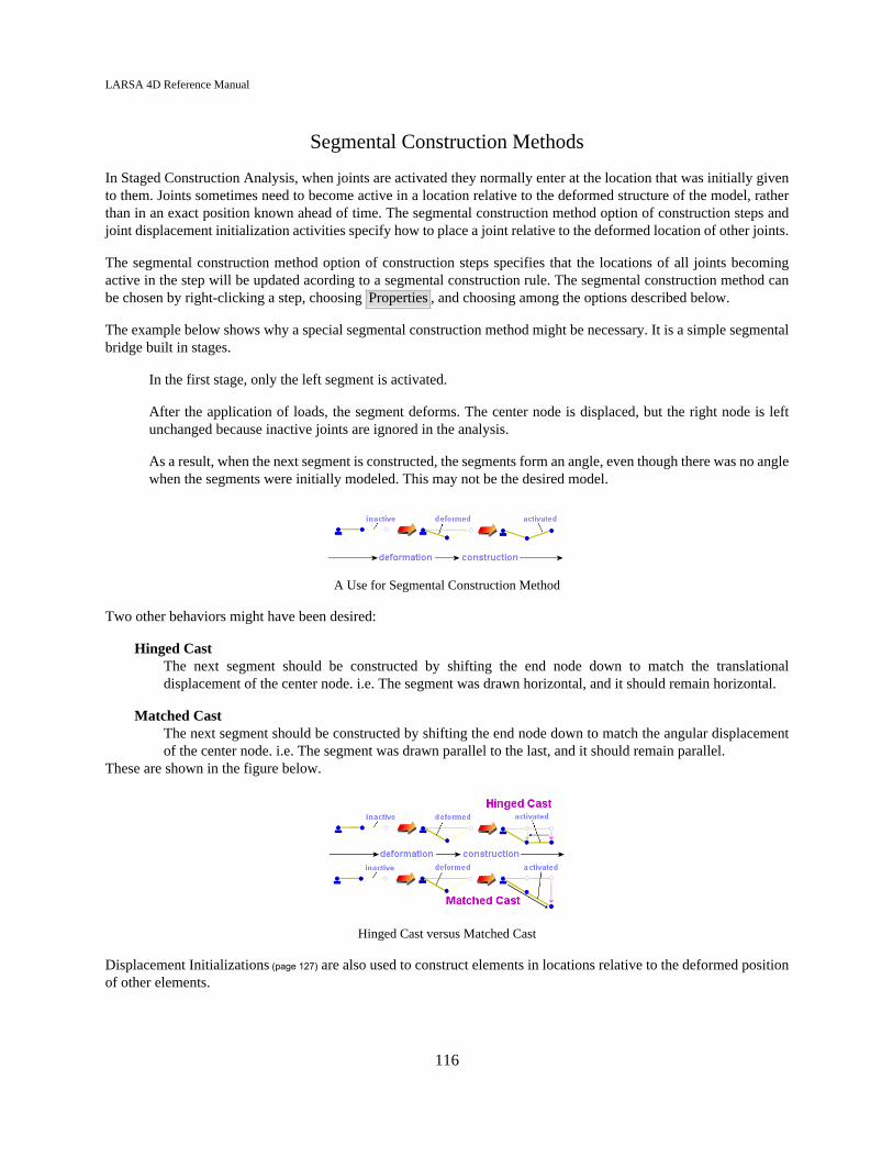
LARSA 4D Reference Manual
Segmental Construction Methods
In Staged Construction Analysis, when joints are activated they normally enter at the location that was initially givento them. Joints sometimes need to become active in a location relative to the deformed structure of the model, ratherthan in an exact position known ahead of time. The segmental construction method option of construction steps andjoint displacement initialization activities specify how to place a joint relative to the deformed location of other joints.
The segmental construction method option of construction steps specifies that the locations of all joints becomingactive in the step will be updated acording to a segmental construction rule. The segmental construction method canbe chosen by right-clicking a step, choosing Properties , and choosing among the options described below.
The example below shows why a special segmental construction method might be necessary. It is a simple segmentalbridge built in stages.
In the first stage, only the left segment is activated.
After the application of loads, the segment deforms. The center node is displaced, but the right node is leftunchanged because inactive joints are ignored in the analysis.
As a result, when the next segment is constructed, the segments form an angle, even though there was no anglewhen the segments were initially modeled. This may not be the desired model.
A Use for Segmental Construction Method
Two other behaviors might have been desired:
Hinged CastThe next segment should be constructed by shifting the end node down to match the translationaldisplacement of the center node. i.e. The segment was drawn horizontal, and it should remain horizontal.
Matched CastThe next segment should be constructed by shifting the end node down to match the angular displacementof the center node. i.e. The segment was drawn parallel to the last, and it should remain parallel.
These are shown in the figure below.
Hinged Cast versus Matched Cast
Displacement Initializations (page 127) are also used to construct elements in locations relative to the deformed positionof other elements.
116

LARSA 4D Reference Manual
For More Information, please refer to the following documentation.
• Staged Construction Analysis on page 205.
• Geometry on page 45.
• Construction Stages Explorer in LARSA 4D User’s Manual.
• Structure Groups Explorer in LARSA 4D User’s Manual.
• Displacement Initializations on page 127.
117

LARSA 4D Reference Manual
118
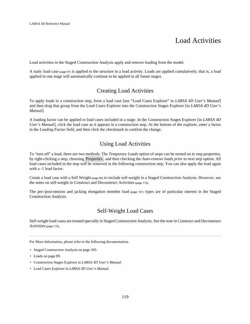
LARSA 4D Reference Manual
Load Activities
Load activities in the Staged Construction Analysis apply and remove loading from the model.
A static load case (page 91) is applied to the structure in a load activity. Loads are applied cumulatively; that is, a loadapplied in one stage will automatically continue to be applied in all future stages.
Creating Load Activities
To apply loads in a construction step, form a load case [see “Load Cases Explorer” in LARSA 4D User’s Manual]and then drag that group from the Load Cases Explorer into the Construction Stages Explorer [in LARSA 4D User’sManual].
A loading factor can be applied to load cases included in a stage. In the Construction Stages Explorer [in LARSA 4DUser’s Manual], click the load case as it appears in a construction step. At the bottom of the explorer, enter a factorin the Loading Factor field, and then click the checkmark to confirm the change.
Using Load Activities
To "turn off" a load, there are two methods. The Temporary Loads option of steps can be turned on in step properties,by right-clicking a step, choosing Properties , and then checking the Auto-remove loads prior to next step option. Allload cases included in the step will be removed in the following construction step. You can also apply the load againwith a -1 load factor.
Create a load case with a Self Weight (page 95) to include self-weight in a Staged Construction Analysis. However, seethe notes on self-weight in Construct and Deconstruct Activities (page 115).
The pre-/post-tension and jacking elongation member load (page 101) types are of particular interest in the StagedConstruction Analysis.
Self-Weight Load Cases
Self-weight load cases are treated specially in Staged Construction Analysis. See the note in Construct and DeconstructActivities (page 115).
For More Information, please refer to the following documentation.
• Staged Construction Analysis on page 205.
• Loads on page 89.
• Construction Stages Explorer in LARSA 4D User’s Manual.
• Load Cases Explorer in LARSA 4D User’s Manual.
119

LARSA 4D Reference Manual
120

LARSA 4D Reference Manual
Support and Hoist Activities
Support activities are used to change support conditions in a model during construction. Hoist activities are used tohoist a joint in a direction by the same but opposite amount it deformed.
A support activitiy changes the support conditions of a joint in the model. A hoist activity applies a displacement to ajoint, in one of its six directions of displacement, with a magnitude equal and opposite to the total displacement of thejoint since initial conditions in that direction, and then restrains the joint in that direction.
When a support or hoist activity is applied to a joint, the new support conditions for all six degrees of freedom at thejoint must be specified. In each of the six directions, which as with joint restraints (page 47) are in global directions unlessa joint displacement coordinate system is set on the joint, the joint must be specified as free, fixed, or hoisted.
Do not leave a direction as free to mean that the joint's support conditions have not changed. This will remove a supportin that direction if one was previously specified.
When hoist is chosen in a given direction, the joint is forced to deform back to its initial coordinate in the directionand then is supported in that direction.
When a support is removed, by changing a direction to free if the joint was already supported in that direction, thereactions at that joint are applied back into the model. See Load Class Tracking (page 221).
Activity Fields
JointThe ID of the joint whose support conditions are changing.
X/Y/Z-Translation and X/Y/Z-RotationThe new support condition of the joint in each direction: free, fixed, or hoist. These are described above.
For More Information, please refer to the following documentation.
• Staged Construction Analysis on page 205.
• Construction Stages Explorer in LARSA 4D User’s Manual.
• Joints on page 47.
121

LARSA 4D Reference Manual
122

LARSA 4D Reference Manual
Slave/Master Change Activities
Slave/master activities in the Staged Construction Analysis apply and remove slave/master restraints between degreesof freedom of two joints.
Like the Slave/Master Constraints (page 73) specified for other analysis types and for initial conditions in the StagedConstruction Analysis (page 205), slave/master activities are used to manage equal-displacement constrained behaviorbetween two degrees of freedom in the model. A slave/master activity adds or removes such constraints during a stepof construction.
When a slave/master activity is applied to a slave joint, the conditions of each of that joint's six degrees of freedommust be specified. A condition for a direction can be left as (none) when the joint is free to move in that direction, orthe ID number of a so-called "master" joint can be specified to ensure that displacements in that direction are equalbetween the master and the slave.
Do not leave a condition field (master joint ID) as (none) to mean that the slave conditions do not change in the step.Leaving a field as (none) means that the joint becomes free in that direction in the step.
If a slave/master constraint is removed through an activity, the new unbalanced forces from the elements on the jointare added back into the structure. See Load Class Tracking (page 221).
Activity Fields
Slave JointThe joint ID of the slaved joint.
Master Joint for X/Y/Z-Translation and X/Y/Z-RotationIf a Joint ID is specified, then the displacement in this direction of the slave joint will be equal the displacementin the same direction as this master joint. If no joint ID is speicified, then the displacement in this direction ofthe slave joint is free.
For More Information, please refer to the following documentation.
• Staged Construction Analysis on page 205.
• Slave/Master Constraints on page 73.
• Construction Stages Explorer in LARSA 4D User’s Manual.
123

LARSA 4D Reference Manual
124

LARSA 4D Reference Manual
Tendon Stressing and Slackening Activities
Tendon stress/slacken activities apply or remove the effect of pre- and post-tensioning tendons (page 75) in the model.
The effect of Tendons (page 75) defined in the model is not applied until they are stressed in a Staged ConstructionAnalysis (page 205) activity. A tendon stressing activity indicates that the equivalent loading representing the tendonis to be added into the model.
If a Time-Dependent Staged Construction Analysis is run and the appropriate time-dependent effects are selected,these effects on tendons will be automatically included in the results. See Time Effects on Materials (page 217).
It is also possible to slacken a tendon by choosing Slacken as the activity type.
Activity Fields
TendonThe tendon being stressed or slackened.
ActivityStress or Slacken
For More Information, please refer to the following documentation.
• Staged Construction Analysis on page 205.
• Tendons on page 75.
• Construction Stages Explorer in LARSA 4D User’s Manual.
125

LARSA 4D Reference Manual
126

LARSA 4D Reference Manual
Displacement Initializations
Displacement initialization construction activities specify that a joint's location should be updated based on thedisplacements of one or two other joints or a fixed offset.
When joints are constructed at different times, geometrical relationships between joints may be altered due todisplacements in the model. For instance, although three joints may be colinear in initial conditions specified inthe geometry spreadsheet, displacement at two of the joints before the third is constructed may alter that geometricrelationship. When the third joint is constructed, the members connecting the joints may form an angle rather than astraight line. This is depicted in the figure below.
A Use for Displacement Initializations
Displacement initializations are used to update the initial conditions of a joint before it is constructed based on thedisplacement of one or two other joints. Displacement initializations can also be used to specify an exact geometryupdate so that the joint coordinates in the joints spreadsheet (page 47) can be overridden in Staged Construction Analysis.
Displacement initializations cannot be used in the first construction step.
See also the segmental construction methods (page 115) for other options to update joint coordinates based ondisplacement during Staged Construction Analysis.
What It Does
One slave and up to two master joints are specified. The slave joint is the non-constructed joint whose location is to beupdated. The master joint(s) are already constructed and probably have had displacement by the time of the previousconstruction step.
If no master joints are specified, then the slave joint's coordinates are updated by adding in the values in theDisplacement X/Y/Z columns.
If one master joint is specified, or if two master joints are specified but they are coincident in initial conditions, thenthe slave joint's location is updated by adding to it the total displacement of the (first) master joint at the end of theprevious construction step, plus any additional displacement entered into the Displacement X/Y/Z columns.
If two master joints are specified and they are not coincident in initial conditions, then the slave joint's location isupdated by adding to it a linear interpolation between the two master joint's total displacements at the end of theprevious construction step, plus any additional displacement entered into the Displacement X/Y/Z columns. If thethree joints are colinear in initial conditions (master 1--slave--master 2), then the interpolation is simply linear alongthat line. For instance, if the slave is mid-way between the two master joints, then it will be adjusted by an amount
127

LARSA 4D Reference Manual
equal to the average of the two displacements. However, in the general case, the interpolation is linear using the ratioof the distance between the first master and the slave to the distance between the two master joints.
The Direction column limits the update to only certain components of the slave joint's location. If the Direction isall, the coordinate update is as describe above. If the Direction is y, for instance, then the x- and z-components of thecomputed slave joint displacement are reset to zero.
Activity Fields
JointThe ID of the slave joint whose location is to be updated.
Master Joint 1/2The zero, one, or two master joints whose displacements in the previous construction step are used to adjust thelocation of the slave joint.
DirectionThe translational degrees of freedom of the joint to update. Select all to update the joint normally. Or, forexample, specify just x to update the joint's x location only, leaving its y and z coordinates unchanged.
Displacement X/Y/ZAdditional displacement values to apply to the slave joint. Displacements in directions that are not specified inthe Direction column are ignored.
For More Information, please refer to the following documentation.
• Staged Construction Analysis on page 205.
• Construction Stages Explorer in LARSA 4D User’s Manual.
• Construct and Deconstruct Activities on page 115.
• Joints on page 47.
128
LARSA 4D Reference Manual
Analysis Scenarios
Analysis Scenarios are analyses performed during a Staged Construction Analysis (page 205), such as a live load analysisor pushover, based on the deformed state of the structure at any time.
Any time of analysis can be performed in a construction step. To change the analysis type, right-click the constructionstep and choose Properties . Then at the bottom right of the window, choose the analysis type.
You will also need to add a load case into the construction step as a load activity (page 119) that specifies the parametersfor the scenario. For instance, for a live load (moving load or influence) scenario, include a load case with a movingload or influence set-up load.
For More Information, please refer to the following documentation.
• Staged Construction Analysis on page 205.
• Construction Stages Explorer in LARSA 4D User’s Manual.
• Load Cases Explorer in LARSA 4D User’s Manual.
129

LARSA 4D Reference Manual
130
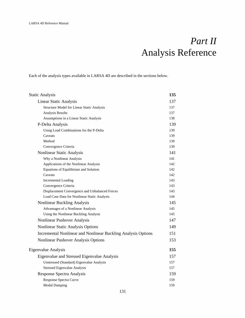
LARSA 4D Reference Manual
Part IIAnalysis Reference
Each of the analysis types available in LARSA 4D are described in the sections below.
Static Analysis 135
Linear Static Analysis 137Structure Model for Linear Static Analysis 137
Analysis Results 137
Assumptions in a Linear Static Analysis 138
P-Delta Analysis 139Using Load Combinations for the P-Delta 139
Caveats 139
Method 139
Convergence Criteria 139
Nonlinear Static Analysis 141Why a Nonlinear Analysis 141
Applications of the Nonlinear Analysis 142
Equations of Equilibrium and Solution 142
Caveats 142
Incremental Loading 143
Convergence Criteria 143
Displacement Convergence and Unbalanced Forces 143
Load Case Data for Nonlinear Static Analysis 144
Nonlinear Buckling Analysis 145Advantages of a Nonlinear Analysis 145
Using the Nonlinear Buckling Analysis 145
Nonlinear Pushover Analysis 147
Nonlinear Static Analysis Options 149
Incremental Nonlinear and Nonlinear Buckling Analysis Options 151
Nonlinear Pushover Analysis Options 153
Eigenvalue Analysis 155
Eigenvalue and Stressed Eigenvalue Analysis 157Unstressed (Standard) Eigenvalue Analysis 157
Stressed Eigenvalue Analysis 157
Response Spectra Analysis 159Response Spectra Curve 159
Modal Damping 159
131

LARSA 4D Reference Manual
Modal Combination 160
Spatial Combination 160
Ground Motion Directions 160
Response Spectra Load Cases 161
Caveat About Sign 162
Analysis Options for Response Spectra 162
Eigenvalue Analysis Options 163
Stressed Eigenvalue Analysis Options 165
Time History Analysis 167
Linear Time History Analysis 169Time History Load Cases 169
Applied Loads 169
Nonlinear Time History Analysis 171Overview 171
Newmark-Beta with Newton-Raphson 171
Sparse Solver Technology 171
Nonlinear Time History Data 171
Time History Analysis Options 173
Nonlinear Time-History Analysis Options 175Geometric Nonlinearity 175
Live Load Analysis 177
Moving Load Analysis 179Vehicle Paths: Lanes 179
Load Cases for Moving Load Analysis 179
Influence Line & Surface Analysis 181
Influence Analysis Overview and Options 183The Assumption of Linearity 183
The Vehicle Loading Algorithm 183
Performing an Influence Analysis 184
General Loading Parameters 185
Vehicular Loading Options 187
Vehicular Options for the 7.01 Compatible Solution Method 190
Uniform/Patch Loading Options 190
Procedure: Getting Results 190
Suggestions for Influence Analysis 193Suggestions for Speed 193
Influence Surfaces in LARSA 4D Version 7.01 195Design Lane Options 195
Vehicle Type and Placement Options 196
AASHTO LFD Point Loading in LARSA 4D Version 7.01 197
Standard Vehicles 199AASHTO and CALTRANS Vehicles 199
132

LARSA 4D Reference Manual
AASHTO Load Patterns for Influence Analysis 199
IRC Load Patterns for Influence Analysis 200
Moving Load Analysis Options 203
Staged Construction Analysis 205
Overview of Staged Construction Analysis 207
Staged Construction Activities 209
Setting Up the Model 211Preparation 211
Creating Activities in the Explorer 212
Creating Activities in the Stage Editor 213
Time Effects on Materials 217Definitions 217
General Options 218
Load Class Tracking 221Setting up the model 221
The Load Classes of Result Cases 221
Accessing Class-Based Results 222
Staged Construction Analysis Options 223Options for Analysis Scenarios 224
Solver Options 227
133

LARSA 4D Reference Manual
134
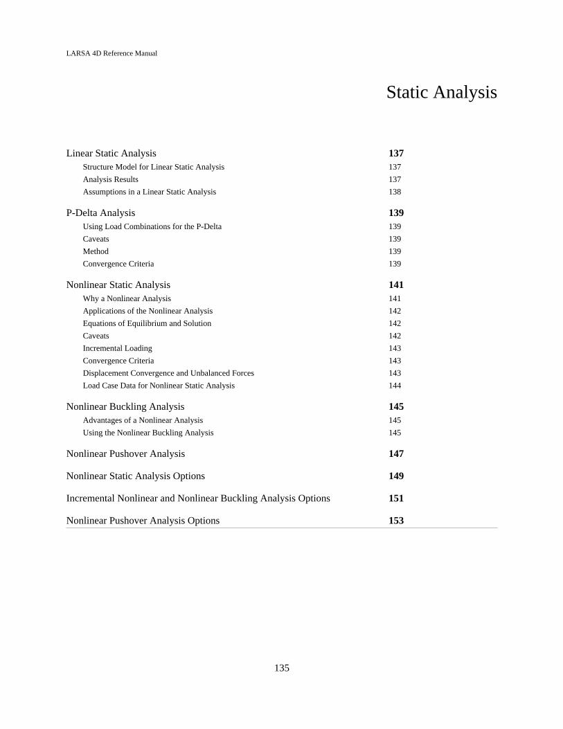
LARSA 4D Reference Manual
Static Analysis
Linear Static Analysis 137Structure Model for Linear Static Analysis 137
Analysis Results 137
Assumptions in a Linear Static Analysis 138
P-Delta Analysis 139Using Load Combinations for the P-Delta 139
Caveats 139
Method 139
Convergence Criteria 139
Nonlinear Static Analysis 141Why a Nonlinear Analysis 141
Applications of the Nonlinear Analysis 142
Equations of Equilibrium and Solution 142
Caveats 142
Incremental Loading 143
Convergence Criteria 143
Displacement Convergence and Unbalanced Forces 143
Load Case Data for Nonlinear Static Analysis 144
Nonlinear Buckling Analysis 145Advantages of a Nonlinear Analysis 145
Using the Nonlinear Buckling Analysis 145
Nonlinear Pushover Analysis 147
Nonlinear Static Analysis Options 149
Incremental Nonlinear and Nonlinear Buckling Analysis Options 151
Nonlinear Pushover Analysis Options 153
135

LARSA 4D Reference Manual
136

LARSA 4D Reference Manual
Linear Static Analysis
The linear elastic static analysis is a first order analysis that excludes nonlinearity.
The following are the basic assumptions:
• Materials are assumed to be elastic and unyielding with their properties invariable.
• The equations of equilibrium are formulated on the geometry of the unloaded structure.
• The deformations are assumed to be so small as to be insignificant in their effect on the equilibrium.
• Strains are small and stresses are proportional to strains.
Linear static analysis can compute the response of the structure to various types of static loads in the form of selfweight, joint loads, joint displacements, loads applied to beam elements, thermal loads applied to beam, truss, andcable elements, and surface and thermal loads applied on plate and shell elements.
Linear static analysis is performed on load cases (page 91) whose types are set to Static and factored combination of theseload cases (load combinations (page 93)). The load conditions are solved simultaneously in a single solution.
Structure Model for Linear Static Analysis
In the linear static analysis, the structure must include only linear elements. Cable and compression only foundationspring elements are examples of nonlinear elements that cannot be used in the linear static analysis. If nonlinearelements are used in the structure model while performing linear static analysis, LARSA will replace these elementswith their equivalent linear elements on-the-fly without modifying the model data. For example, a cable element isautomatically replaced by a truss element in linear static analysis.
Here is a list of nonlinear elements that are replaced with their linear equivalent if used in a linear static analysis:
• Cable Element
• Tension-Only and Compression-Only Truss Elements
• Grounded Spring Element with different stiffness for tension and compression
• One- or Two-Node Spring Element with a nonlinear spring property definition
• Hysteretic Beam Element
• Connection Beam Element
• Hysteretic Spring Element
• Seismic Isolator and Bearing Elements
Analysis Results
Typical results from the linear static analysis are:
• Joint displacements
• Reaction forces at support joints
• Member end forces in global XYZ or in member local directions
137

LARSA 4D Reference Manual
• Member sectional forces, stresses, and displacements
• Plate center forces and stresses, and joint forces
• Spring forces
Assumptions in a Linear Static Analysis
By definition, the linear elastic static analysis is a first order analysis that excludes both geometric and materialnonlinearity. In practical terms the assumptions of this analysis means:
• The geometry of the elements remains unchanged during the loading.
• First order, infinitesimal, and linear strain approximations can be used.
• The material behavior of the elements is linear.
When the acceleration dependent inertia forces and velocity dependent damping forces are ignored, the equations ofequilibrium for static analysis are reduced to the following:
Kt U = RwhereU = Joint displacement vectorR = Applied joint force vectorwith the tangent stiffness matrix, in the following form:Kt = Ko + Kg + Ks
where
• Kt = Tangent stiffness
• Ko = Small displacement stiffness
• Kg = Large displacement stiffness for geometry change
• Ks = Geometric stiffness (stress stiffening)
In the linear static analysis, the displacements are assumed small, the effect of stress stiffening is ignored, and materialbehavior is assumed linear elastic. Therefore, the stiffness due to the change of geometry (Kg) and stress stiffening(Ks) are not considered. Then tangent stiffness matrix (Kt) becomes the same as the stiffness matrix corresponding tolinear small displacement behavior:
Kt= Ko
It should be noted that for the linear analysis, the terms in the stiffness matrix are constant values and do not depend onthe unknown displacements. The equilibrium equations are linear simultaneous equations and the closed-form solutionis obtained directly for the unknown joint displacements. The element end forces are computed by simply multiplyingthe element end deformations by the element stiffness matrix.
For More Information, please refer to the following documentation.
• Running an Analysis in LARSA 4D User’s Manual.
138

LARSA 4D Reference Manual
P-Delta Analysis
If the loads applied to the structure change the geometry and stiffness, the first order linear elastic static analysis maynot be satisfactory. It is then recommended to use some form of nonlinear analysis where second-order effects areconsidered. P-Delta is the most basic type of second order or nonlinear analysis.
The P-Delta can be defined as the secondary effect of column axial loads and lateral deflections on the moments inmembers. These effects can be separated as:
• A destabilizing moment equal to a gravity load times the horizontal displacement it undergoes as a result ofthe lateral displacement of the supporting structure.
• The influence of axial force on the flexural stiffness of individual members.
The most common situation where a second-order effect must be considered is a multi-story building under lateralloading (wind and/or earthquake) that must rely on the stiffness of the beams and columns to resist sway. A membersubjected to a large axial force combined with transverse loads or to transverse end translation or rotation represents atypical P-Delta or geometric nonlinear problem.These type of second-order effects are often referred to as the beam-column problem, or a P-Delta problem.
Using Load Combinations for the P-Delta
When performing a P-Delta analysis, only active load combinations will be analyzed. The load cases within the loadcombination must be static load cases. The load combinations are solved separately but within a single analysis run.
The load cases are applied incrementally in the same order as entered in the load combination data. For the loadcombination 1.2*(Dead Load) + 1.6*(Live Load), LARSA will first apply and solve for the load vector as 1.2 timesDead Load and after convergence is established, 1.6 times the live load is applied and solved for.
Caveats
P-Delta analysis should not be used as a substitute for a nonlinear static analysis for any type of cable structure suchas suspension bridges, cable-stayed bridges, and other cable structures like stadium roofs or guyed towers.
Method
The method for P-Delta in LARSA is the same method employed in all nonlinear analysis options but with a limitednumber of iterations and without any nonlinear elements. The method used here is the iterative full Newton-Raphsonmethod, updating the tangent stiffness matrix in every iteration for the P-Delta effects. The equilibrium at the joints arebased on the deformed shape of the elements in the structure. Therefore, the P-Delta effects are incorporated directlyinto the stiffness matrix as part of the geometric stiffness including geometry change and stress-stiffening.
Convergence Criteria
The Displacement Tolerance, Force Tolerance, and Maximum Number of Iterations are the basic convergence criteriaspecified in any of the nonlinear static analysis based options. However, for the P-Delta analysis, these values arepreset.
139
LARSA 4D Reference Manual
The Displacement Tolerance is the ratio of the incremental displacement computed in the last iteration to the totaldisplacement for the same degree of freedom. This criteria is set to 0.01 (1%) for P-Delta.
The Maximum Number of Iterations is the maximum number of iterations that can be performed for each load step.The value is set to 5 for P-Delta. The iterative analysis continues untill all degrees of freedom in the model satisfyDisplacement Tolerance of 0.01 but up to the maximum 5 iterations.
If the solution for a load step within a load combination is not convergent when number of iterations performed isequal or exceeds the maximum specified, a message is displayed on the screen and captured in the run log reportingnonconvergence. If there are additional load steps for the same load combination, analysis will continue if the structurehas not become unstable. The unbalanced forces are carried into the next load step and a convergent solution may beobtained in the next load step. This may imply that your structure is fine and you either have to use smaller factoredload steps within the load combinations or use a nonlinear static analysis where the user can increase the maximumnumber of iterations or use less restrictive tolerances.
For More Information, please refer to the following documentation.
• Running an Analysis in LARSA 4D User’s Manual.
140

LARSA 4D Reference Manual
Nonlinear Static Analysis
In structures, nonlinearity can be classified as material nonlinearity or as geometric nonlinearity. Material nonlinearityis associated with changes in material properties: inelastic behavior. Geometric nonlinearity is associated with changesin configuration, such as large deflections of a slender elastic beam or structures with cables.
The nonlinear static analysis takes into account geometric and material nonlinearity by iteratively solving for thedisplacements of a structure, stopping when convergence criteria have been met.
Deformations can significantly alter the location or distribution of loads so that equilibrium equations must be writtenwith respect to the deformed geometry, which is not known in advance. One seeks a displacement state in which thedeformed structure is in equilibrium with the loads applied to it.
Geometric nonlinearity in LARSA includes both the change in geometry and the effects of stress stiffening such asthat encountered when a cable or a thin member is stressed in tension or in compression.
Structures can include several types of material nonlinearities at the element level. The inelastic beam element (ahysteretic beam element based on spread plasticity using a yield surface), the connection beam element with inelasticrotational connection springs, the nonlinear elastic and nonlinear inelastic springs, gap and hook elements, andfoundation springs with nonlinear elastic or inelastic material behavior all exhibit these properties.
The nonlinear static analysis takes into consideration the following:
• Large displacements. The stiffness matrices of the elements are based on deformed geometry.
• Stress stiffening due to the internal axial forces in beam, truss, and cable elements, but not plate elements.
• Effects of follower forces from joint loads due to displaced geometry.
• Gaps and hooks which open, close, and slide.
• Nonlinear elastic and inelastic material behavior of spring elements.
• Compression-only grounded springs with zero stiffness when open.
• Yield force capacity in foundation elements.
• Inelastic material behavior in beam elements using tri-axial yield surfaces.
• Ability to have plastic hinges along the member length without specifying locations.
• Different paths during post-yield.
• Plastic moment capacity in beams.
Why a Nonlinear Analysis
It is fortunate that the linear analysis based on linear approximations works quite well for many problems in structures.In a linear analysis, the material is assumed to be unyielding and its properties invariable, and the equations ofequilibrium are formulated on the geometry of the unloaded structure.
Although most analyses and designs stay within the linear elastic range, many physical situations present nonlinearities,and more and more structures demand that nonlinearities be considered for more accurate analysis and design. Slenderstructures such as suspension systems, arches, tall buildings, and structures subject to local yielding and cracking arebasic types among structures requiring nonlinear analysis.
141

LARSA 4D Reference Manual
The fundamental goal of using the nonlinear analysis is to improve the quality of design with a more reliable predictionof performance of a structure. Nonlinear analysis can help us reduce the uncertainty regarding actual behavior ofa structure. Meanwhile, the effort for modeling the structure and handling the equations of analysis is significantlyincreased.
Applications of the Nonlinear Analysis
Suspension bridges, cable-stay bridges, and cable domes are structures with high geometric nonlinearity. Thesestructures are complex in shape, and usually the final deformed shape of the structure is given. The analysis involvesfinding the initial shape of the structure along with the prestress forces to be applied to bring the structure to its finalshape under given loading conditions. The analysis needs to consider the deformed geometry and the stress stiffeningeffects.
Similarly, for the computation of the eigenvalues and mode shapes for suspension bridges and similar structures, theeffects of large displacements and stress stiffening need to be considered. Neglecting the nonlinear effects may resultin incorrect values for natural frequencies of the structure.
Consider foundations and bridge piers. These structures are usually supported by soil or friction bearing piles whichmay not sustain tensile forces. The model for these structures may consist of a combination of beam and plate elementsrepresenting the bridge structure. The piles and soil can be represented using the nonlinear foundation elements. Thestiffness of the foundation elements will depend on the displacements. The solution can be obtained in one singleanalysis run using the nonlinear analysis.
Many of the seismic design and analysis procedures for bridges require consideration of nonlinear behavior. Thesemethods assume plastic hinges will form to utilize the full displacement capacity during an earthquake. Abutments,hinges, and restrainers in bridge structures are nonlinear elements. Abutments and hinges can transfer only load incompression. Restrainers transfer only load in tension. Nonlinear analysis is a more reasonable tool to use than a seriesof linear analyses for these types of analyses.
Plastic deformations of steel structures, cracking or creep of reinforced concrete structures, inelastic interaction ofaxial force and bending moments, connection deformations, and panel zone deformations are among the many sourcesof nonlinearity. Rarely is it possible to model all sources of nonlinearity for a practical structure. Normally, the goalis to choose a model that does provide adequate analytical simulation of the actual behavior.
Equations of Equilibrium and Solution
In a nonlinear analysis, the equilibrium equations are formulated with respect to the deformed geometry of the structure,which is not known in advance and will change with the applied loads. The stiffness matrix depends on the unknowndisplacements. The result is a set of nonlinear simultaneous equations. It is necessary to employ an iterative technique toobtain a solution in nonlinear analysis. An iterative scheme based on Newton-Raphson Method has been implementedin LARSA.
Caveats
Using nonlinear analysis is not difficult, but misuse of it without understanding the methodology may lead to disasters.It is always a good practice to explore and understand the implementation of the nonlinear analysis in the computerprogram that is used. Users should always keep in mind that a nonlinear analysis may not have a unique solution aswith the linear analysis. Therefore, any solution obtained must be verified by the user. We recommend the user knows:
• Sources of nonlinearity that are significant.
142

LARSA 4D Reference Manual
• How to represent these nonlinearities in the model.
• The formulation of the element stiffness matrices: tangent, secant or initial.
• The material nonlinearity formulation of the elements.
• The solution technique used - Full or Modified Newton-Raphson.
• How convergence criteria are satisfied.
• The number of iterations required for convergence.
• The magnitudes of unbalanced forces on the structure.
Incremental Loading
It must be kept in mind that in computing displacements for a given set of loads within a range of nonlinear behavior,it is essential to apply the loads incrementally. In general, it may not be possible to start from the unloaded state andapply the total loading in a single step due to numerical instabilities in the solution of the simultaneous equations.
The user must be cautioned that the solutions for nonlinear analyses are not direct closed form solutions as in linearanalysis. Any loading causing abnormal displacements may not result in convergence.
The computed displacements, reactions and element forces at the end of any load step are the accumulated effectsfrom all the load steps considered.
Convergence Criteria
The convergence criteria are specified by the user as the tolerable error ratio for displacement, maximum unbalancedforce and maximum number of iterations. The tolerable error ratio is the incremental displacement computed in thelast iteration divided by the total displacement for the same degree of freedom. The default value is 0.001 (0.10%). Theiterative analysis continues untill all degrees of freedom in the model satisfy both criteria. However, the number ofiterations performed for each load step is limited not to exceed the maximum number of iterations specified by the user.
If the solution is not convergent for a load step, a message is displayed on the screen. If there are additional load steps,analysis continues as long as the structure is not unstable. LARSA carries the unbalanced forces into the next load stepand a convergent solution may be obtained in the next load step. This may imply that your structure model is fine andyou either have to increase the maximum number of iterations or use a less restrictive error ratio.
Displacement Convergence and Unbalanced Forces
The displacement convergence and unbalanced force reports include important information in evaluating the resultsof the nonlinear analysis. These reports are used for accepting the convergence of the results for the solution.Thedisplacement convergence report provides the maximum error in the displacements during each iteration. Theunbalanced force report tells us the error about the internal force equilibrium of the structure.
The structure must be in equilibrium for a convergent solution. When any unbalanced force remains, the structure isnot in equilibrium. The unbalanced forces at the end of each load step are recorded in the log file. The report includesthe joints with significant unbalanced forces and summarizes the maximum and total unbalanced force vector for allsix DOF in the structure.
It is imperative that the user comprehend the information provided in these reports. In the best case, both reports haveall zeros.
143

LARSA 4D Reference Manual
Load Case Data for Nonlinear Static Analysis
In LARSA, the nonlinear static analysis can be performed for:
• Computing the response of the structure to several load cases.
• Computing the response of the structure to several independent factored load cases.
• Tracing the load-deflection response of the structure.
Most of the nonlinear analysis falls in the second category where the response of the structure is computed for severalload combinations in the same run. The complete load-deflection response of the structure to a series of incrementalloads is required in a pushover analysis (page 147) or in a nonlinear buckling analysis (page 145).
The load cases and applied loads are defined exactly in the same manner as for the linear static analysis.
For More Information, please refer to the following documentation.
• Nonlinear Static Analysis Options on page 149.
• Nonlinear Buckling Analysis on page 145.
• Nonlinear Pushover Analysis on page 147.
144

LARSA 4D Reference Manual
Nonlinear Buckling Analysis
The nonlinear buckling analysis provides an accurate indication of the loads that will cause a structure to fail. Theanalysis traces the deformation of the structure using incremental load applications until the structure becomes unstable.After the analysis, load-deformation curves throughout the structure show the nature of buckling leading up to collapse.
Buckling occurs when compressive membrane forces in elements are large enough to cause a reduction in bendingstiffness. In beam-column elements, this is when compressive axial force reduces bending stiffness. In plates, bucklingoccurs when in-plane forces reduce out-of-plane stiffness.
This analysis effectively plots load versus displacements for all parts of the structure up to collapse. The slope of theseplots indicates how different parts of the structure are buckling before collapse. Just before buckling, small changesin force will yield rapid deformations.
Collapse occurs when the stiffness matrix of the structure becomes singular and thus unsolvable. A singular matrixindicates the structure has no predictable deformation under any loading. Analysis stops at this point.
Advantages of a Nonlinear Analysis
The nonlinear buckling analysis provides a more accurate indication of buckling than other methods. A linearbifurcation buckling analysis, usually based on eigenvalue solutions, oversimplifies buckling behavior and often under-or over-estimates buckling conditions. A linear analysis cannot account for important nonlinearities in a structurethat play a crucial role in buckling. For instance, post-buckling strength in inelastic elements could not be accountedfor, and the effects of changes in geometry and load directions are also ignored. By applying small load incrementsin a nonlinear analysis, the nonlinear buckling analysis accurately computes the effect of buckling as the structureapproaches collapse.
Using the Nonlinear Buckling Analysis
The nonlinear buckling analysis is usually performed by first applying loads known not to cause buckling, and thenincrementally applying additional loads until further analysis cannot be performed because the structure has becomeunstable. Loads are defined in static load cases (page 91).
Appropriate increment sizes depend entirely on the structure and nature of loads. Practically, the increment on the firstcondition should be 1.0 because the first condition should not cause buckling. The next condition may start with afactor of 1.0, and if it causes buckling the factor should be reduced to find the point of collapse. Once the point ofcollapse is known, the final loading condition should be applied in small increments, such as 10 increments of 0.1factors. The increments and number of load applications can then be refined as needed.
When performing the analysis, the analysis engine will treat all load combinations (page 93) in the project cumulatively.Each load combination will be analyzed based on the deformation that occured in the previous combination. Factorswithin the load combinations determine how to incrementally load the structure.
For instance, to apply a load case in 10 increments, create a load combination that includes the static load case to apply.Assign the static load case a factor of 0.1 in the combination, and then repeat the combination 10 times.
Factors need not be equal, and load combinations can be repeated as many times as is necessary to obtain results forthe desired loading conditions.
145

LARSA 4D Reference Manual
For More Information, please refer to the following documentation.
• Nonlinear Static Analysis on page 141.
• Incremental Nonlinear and Nonlinear Buckling Analysis Options on page 151.
146
LARSA 4D Reference Manual
Nonlinear Pushover Analysis
Pushover analysis is the application of a static load case with progressively increasing scale. The pushover analysis isgenerally used along with the response spectra analysis (page 159) for seismic analysis, and can be used for bucklinganalysis as well. It is a nonlinear analysis.
Models analyzed with the pushover analysis usually contain elements with inelastic material properties, such asinelastic members (page 49) and springs (page 65), because the behavior of the model beyond its elastic limits is generallythe interest of the analysis. For example, plastic hinges can be modeled with inelastic hysteretic springs. Elastic beamswith yielding end connections can be modeled with the connection beam element, a type of member. When spread ofplasticity with a beam is of interest, the beam can be modeled as a hyseretic beam, which is also a type of member.
The initial load factor is given by the user. The stopping criteria can be specified as a maximum displacement of ajoint in a particular direction.
The analysis engine automatically chooses load factor increments based on auto-stepping and arc-length options. Theuser can specifiy the minimum and maximum step size. The maximum step size will be used except when the solutiondoes not converge or it converges too slowly, in which case smaller step sizes are used.
For More Information, please refer to the following documentation.
• Nonlinear Pushover Analysis Options on page 153.
• Nonlinear Static Analysis on page 141.
147

LARSA 4D Reference Manual
148

LARSA 4D Reference Manual
Nonlinear Static Analysis Options
Solution Convergence
Equilibrium iterations at a given load level can cease when the result is "close enough" according to one or morecriteria. Two criteria used in LARSA are that the unbalanced force be a small fraction of the total applied force in thecurrent load level and that the current displacement increment be a small fraction of the displacement increment. Theconvergence criteria are specified by the user as the displacement tolerance, force tolerance and maximum number ofiterations. The iterative analysis continues untill all degrees of freedom in the model satisfy displacement and forcetolerance criteria within the maximum number of iterations.
If the solution is not convergent for a load step, a message is displayed on the screen. If there are additional load steps,analysis will continue if the structure is not unstable. LARSA carries the unbalanced forces into the next load step anda convergent solution may be obtained in the next load step. This may imply that your structure is fine and you eitherhave to increase the maximum number of iterations or use a less restrictive error ratio.
Max # of IterationsThe number of iterations performed for each load step will not exceed the maximum number of iterationsspecified by the user. We recommend 10 to 20 as a maximum number of iterations.
Displacement ToleranceThe displacement tolerance is the error ratio of the incremental displacement computed in the last iterationdivided by the total displacement for the same degree of freedom. The default value is 0.001 (0.10%).
Force ToleranceThe force tolerance is the maximum unbalanced force at any degree of freedom.
Analyze For
Nonlinear static analysis can be performed for load cases and for load combinations in the same analysis run.
Analyze Load CasesIf this option is checked, nonlinear static analysis is performed for all active load cases.
IncrementsWhen analyzing load cases, each load case is the divided into this many equal load steps.
Analyze Load Combinations
The nonlinear static analysis is performed for each load combination by accumulating the loads on the structurein the same sequence as specified in the load combination data.
For More Information, please refer to the following documentation.
• Nonlinear Static Analysis on page 141.
• Running an Analysis in LARSA 4D User’s Manual.
149

LARSA 4D Reference Manual
150

LARSA 4D Reference Manual
Incremental Nonlinear and Nonlinear BucklingAnalysis Options
The Incremental Nonlinear Analysis is used for computing the load-deflection response of the structure as in the plasticpush-over or nonlinear buckling analysis. It can also be used as a simplified staged construction analysis.
Solution convergence control from the nonlinear static analysis (page 149) applies to this analysis type as well.
Load Combinations
In this analysis option, all active load combination cases are treated as load increments. A nonlinear static analysis isperformed by accummulating the loads on the structure in the same sequence as specified from all load combinations.LARSA starts with the load cases specified for the starting load combination and performs nonlinear static analysisfor all load combination steps until it reaches the ending load combination.
For example, a push-over analysis will be performed on a structure to compute the nonlinear load-deflection responseof the structure as the lateral loads are incremented by 10% after its dead load is applied. We want to have the resultsfor the following load combinations:
• Dead
• Dead + 10% Lateral
• Dead + 20% Lateral
• Dead + 30% Lateral
• Dead + 40% Lateral
The load combination data for this problem will be specified as shown below:
Description Case FactorDead Dead 1.0Dead + 0.10*Lateral Lateral 0.10Dead + 0.20*Lateral Lateral 0.10Dead + 0.30*Lateral Lateral 0.10Dead + 0.40*Lateral Lateral 0.10
This load combination data will instruct the program to do the following sequence of load applications in RestartNonlinear Static:
• Load combination 1 (Step 1) - apply 100% of 'Dead'.
• Load combination 2 (Step 2) - add 10% of 'Lateral'.
• Load combination 3 (Step 3) - add 10% more 'Lateral'.
• Load combination 4 (Step 4) - add 10% more 'Lateral'.
• Load combination 5 (Step 5) - add 10% more 'Lateral'.
Starting Load CombinationThe nonlinear static analysis starts with loads applied from this load combination case. Normally you willselect the very first load combination in the data as the starting load combination. However the analysis can
151

LARSA 4D Reference Manual
also start from a combination where the previous load combination has been solved in a prior run. There arelimitations on the type of elements that can be used in a restart analysis performed from a previously solvedload combination.
Ending Load CombinationThe analysis is performed for all load combinations including the one specified as the ending one.
For More Information, please refer to the following documentation.
• Nonlinear Static Analysis on page 141.
• Running an Analysis in LARSA 4D User’s Manual.
152

LARSA 4D Reference Manual
Nonlinear Pushover Analysis Options
Solution convergence control from the nonlinear static analysis (page 149) applies to this analysis type as well.
Pushover Stopping Criteria
Analysis will stop based upon the criteria specified here. Select the joint, the direction and the value for maximumdisplacement.
Auto-Increment Options
The pushover analysis is based on automatically incrementing the load vector. Specify here the multipliers for the loadvector that will be used in computing the initial load vector and the incremental load vector limitation.
InitialThis is the factor multiplying the load vector for computing the load to be applied on the structure in the firstload step.
MinimumThe minimum factor multiplying the load vector that is used in any load step. When the iterative analysisrequires reduction in the magnitude of the load vector, the multiplier cannot be smaller than this value.
MaximumThe maximum factor multiplying the load vector that is used in any load step.
For More Information, please refer to the following documentation.
• Running an Analysis in LARSA 4D User’s Manual.
153

LARSA 4D Reference Manual
154
LARSA 4D Reference Manual
Eigenvalue Analysis
Eigenvalue and Stressed Eigenvalue Analysis 157Unstressed (Standard) Eigenvalue Analysis 157
Stressed Eigenvalue Analysis 157
Response Spectra Analysis 159Response Spectra Curve 159
Modal Damping 159
Modal Combination 160
Spatial Combination 160
Ground Motion Directions 160
Response Spectra Load Cases 161
Caveat About Sign 162
Analysis Options for Response Spectra 162
Eigenvalue Analysis Options 163
Stressed Eigenvalue Analysis Options 165
155

LARSA 4D Reference Manual
156

LARSA 4D Reference Manual
Eigenvalue and Stressed Eigenvalue Analysis
The eigenvalue analysis is performed to extract the undamped free-vibration mode shapes and frequencies of astructure. The eigenvalue analysis is important as a precursor to any dynamic analysis because knowledge of thestructure's natural frequencies and modes can help to characterize its dynamic response. The results of an eigenvalueanalysis also help determine the number of modes to be used in a response spectra analysis.
Each eigenvalue-eigenvector pair is called a natural vibration mode of the structure. The modes are identified bynumbers from 1 to n in the order of increasing frequency. The eigenvalue is the square of the circular frequency forthat mode. The cyclic frequency, f, and period, T, of the mode are multiplicative inverses.
The mass matrix automatically includes the mass of members if section area and weight density are provided, and forplates if weight density is provided. No other elements automatically include mass in dynamic analysis. Mass elements(page 71), which are ignored in static analysis, are used to add additional (usually nonstructural) mass for eigenvalueanalysis. It is also possible to compute mass from static loads by putting static loads in a load case (page 91) marked asrepresenting dynamic mass rather than static loading.
When an eigenvalue analysis is performed, the results from a previous eigenvalue analysis are automaticallyoverwritten in the results database.
Unstressed (Standard) Eigenvalue Analysis
When an eigenvalue analysis of the undeformed structure is requested, the stiffness matrix is computed using theundeformed geometry of the structure. Because no loads are applied, stress stiffening is not included. Static load casesare not used in this type of eigenvalue analysis.
Stressed Eigenvalue Analysis
In the stressed eigenvalue analysis, an eigenvalue analysis performed based on a nonlinear static analysis. The stiffnessmatrix includes the effects of static loads (stress stiffening) and the deformed geometry of the structure.
The user selects the load case for which the program performs a nonlinear static analysis. Eigenvalues are extractedbased on the stiffness of the structure after the applied load.
For More Information, please refer to the following documentation.
• Eigenvalue Analysis Options on page 163.
• Stressed Eigenvalue Analysis Options on page 165.
157

LARSA 4D Reference Manual
158

LARSA 4D Reference Manual
Response Spectra Analysis
Response spectra analysis (RSA) is a statistical type of analysis where the peak response of a multi-degree-freedomsystem can be calculated. Results of RSA are not exact but are accurate enough for structural design applications. RSAprovides an estimate for the response of forces and deformations of a structure to shock loading conditions, such asin seismic analysis.
RSA is not a dynamic analysis but a procedure for dynamic analysis, excluding response history. Although this analysisinvolves only static analysis, RSA is still considered a dynamic analysis procedure because it uses the vibrationproperties such as natural frequencies, corrpesponding mode shapes, and modal damping ratios of the structure andthe dynamic characteristics of the ground motion through its response spectrum.
RSA requires the results of an eigenvalue analysis along with a known spectrum to calculate the most likely peakresponses for displacements, forces and stresses that occur in the structure. To perform the response spectra analysis,the natural frequencies and mode shapes are either calculated prior to RSA within the same analysis run or must havealready been computed in a previous run.
The response spectra analysis can be performed using natural frequencies and mode shapes of the undeformed structure(Eigenvalue Analysis) or of the deformed structure subject to loads (Stressed Eigenvalue Analysis).
Response Spectra Curve
Response spectra curves are graphs of the maximum response (displacement, velocity, or accelaration) to a specifiedexcitation for a single degree-of-freedom system. The abscissa of the curve is the natural frequency (or period) of thestructure, and the ordinate is the maximum response.
The construction of these plots requires the solution of single degree-of-freedom systems for a sequence of valuesof the natural frequency and of the damping ratio. Each solution provides only one point of the response spectrumand the task is lengthy to obtain the maximum response value for all frequencies of interest. Once these curves areavailable for the seismic excitation, the RSA is reduced to calculation of the natural frequencies and mode shapes ofthe structure and the use of the response spectra curves.
In general, the user does not develop the response spectra curves but obtains and use them in the program as a databaseof RSA curves. See The Database Editor [in LARSA 4D User’s Manual] and Connecting Databases [in LARSA 4DUser’s Manual].
It is important to note that the values for the abscissa and ordinate of response spectra curves must be positive or zero.The ordinates can be the actual values or values normalized with respect to a ground accelaration of 1.0 g. If the curveordinate is normalized with respect to g, then you must enter the appropriate g value for the curve in the database editor.
Modal Damping
The damping in the structure affects the shape of the response spectra curve and it also affects the coupling betweenthe modes for modal combination when using CQC. The damping in the structure is included in the shape of theresponse spectra curve.
Modal damping is given as either a critical damping ratio or as a modal damping curve. A damping ratio must beentered if the CQC modal combination rule is used.
159

LARSA 4D Reference Manual
Modal Combination
The modal combination rules are for combining the peak modal responses to determine the peak value of the totalresponse. In general, the peaks for modal responses are at different instants and the peak for combined response isat a different instant with no information about when the peak modal values occur. Modal combination rules areapproximations introduced in combining the peaks of all modal responses determined using the earthquake responsespectra.
The absolute sum (ABSSUM) modal combination rule is based on the assumption that all modal peaks occur at thesame instant, ignoring thesign of response. This leads to an upper bound of the peak value of the total response. Thismethod is not popular in structural design because it is usually considered too conservative.
The square-root-of-sum-of-squares (SRSS) modal combination rule, developed by E. Rosenblueth (1951), providesgood response estimates for structures with well-separated natural frequencies. In SRSS, the peak response in eachmode is squared, the squared modal peaks are summed, and the square root of the sum is the estimate of the peaktotal response.
Starting in the late 1960s, there have been several formulations for the complete quadratic combination (CQC)modal combination rule that is applicable to a wider class of structures. CQC eliminates the limitations of SRSS.E. Rosenblueth and J. Elorduy (1969) were the earliest in CQC formulation. However, the most widely used CQCformulation now is by A. Der Kiureghian (1981) and his formulation is used in LARSA.
According to the CQC rule, the product of the modal peak responses of the ith mode and jth mode and the correlationcoefficient relating these 2 modes are summed and the square root of the sum becomes the estimate of the peak totalreponse. The correlation coefficient varies from 0 to 1 with the value as 1 when i and j refer to the same mode. When iis not equal to j, each of the modal peak values may be positive or negative. A cross term is negative when the modalstatic responses assume opposite signs. Therefore, the estimate obtained by the CQC rule may be larger or smallerthan the estimate provided by the SRSS rule.
Spatial Combination
Usually ground excitation occurs simultaneously in three directions (X, Y and Z). The ground excitation for eachdirection can be specified using three independent load cases, and their effects can be combined to yield the resultanteffect. All three excitations can also be specified in the same load case. If more than one ground excitation is specifiedin a load case, you must also select the spatial combination method for combining the results from each direction.The spatial combination method can be SRSS for Square Root of Sum of Squares or ABS for Absolute Sum. If theexcitation is for a single direction, the spatial combination method is ignored.
Ground Motion Directions
Ground motion in up to three directions can be specified in a response spectra load case. The directions usually coincidewith the global x/y/z directions. By default, spectrum curves 1 and 2 are applied in the global x- and y- directions,respectively. The angle parameter specifies a rotation about the global z-axis to change those directions. The thirddirection is always in the direction of the global z-axis.
Generally, only one spectrum curve is applied per load case. If more than one curve is specified, their results arecombined using the spatial combination method specified.
160
LARSA 4D Reference Manual
Response Spectra Load Cases
The computations in response spectra analysis are organized into response cases similar to load cases in a static analysis.Various response cases of ground motion can be defined as separate load cases, and they can be analyzed in a single run.
Before entering the load data for a response spectra case, the database file containing the spectrum curves must beconnected to the project. See Connecting Databases [in LARSA 4D User’s Manual].
Spectrum Curve in Direction 1The response spectra curve describing the ground motion applied in the first direction.
Scale in Direction 1A multiplier applied to the amplitudes on the curve applied in the first direction
Spectrum Curve in Direction 2The response spectra curve describing the ground motion applied in the second direction.
Scale in Direction 2A multiplier applied to the amplitudes on the curve applied in the second direction.
Spectrum Curve in Global ZThe response spectra curve describing the ground motion applied in the global-Z direction.
Scale in Global ZA multiplier applied to the amplitudes on the curve applied in Z.
AngleThe angle in the xy-plane from the global x-axis to the direction of the first spectrum curve, in degrees.
Modal Combination MethodThe modal combination method determines how the modal values are to be combined into final results. Themodal combination options are CQC for Complete Quadratic Combination and SRSS for Square Root of Sumof Squares.
Spatial Combination MethodIf more than one ground excitation is specified in a load case, you must also select the Spatial Combinationmethod for combining the results from each direction. The Spatial Combination Method can be SRSS forSquare Root of Sum of Squares or ABS for Absolute Sum. If the excitation is for a single direction, the SpatialCombination Method is ignored.
Sign ConventionUsually the results from a response spectra analysis are displayed with no signs. However LARSA gives theuser the option to select sign compatible results that are assigned using the sign convention from the mode withlargest mass participation.
Modal Combination SystemSelect the coordinate system for the modal combination of joint results such as reaction forces anddisplacements. Transformations are not mathematically applicable on the results obtained using modalcombinations. For example, reaction forces computed cannot be transformed to obtain the reaction forces inanother set of directions. The displacements and reaction forces at joints assigned displacement coordinatesystems can be displayed in reference to the global coordinate system when the Modal Combination System isselected as "Global" and the same results can be examined in reference to the displacement coordinate systemof the joint when the selection is "Displacement Coordinate System."
161

LARSA 4D Reference Manual
Modal Damping CurveIf the damping is not constant throughout the frequency range of the structure,a curve where the criticaldamping ratio can be defined as a function frequency can be assigned. This curve data is created and savedwithin the same database file as the response spectrum curves.
Critical Damping RatioUsed in CQC based modal combination in computation of correlation coefficients. The value must be thedamping ratio used to develop the response spectra curve used in the load case. The default is 0.05%.
Caveat About Sign
Response spectra analysis combines the maxima of all modes and for all spatial directions. The response maxima ofthe modes are first combined for a given motion in a spatial direction. Then it is followed by a spatial combinationif more than one excitation direction is specified. Due to the nature of the modal and spatial combination methods,sign information is lost in producing results.
The sign of the results is important for many reasons. Without the sign, the deformed shape of the structure can bedisplayed using only node-to-node displacements. The force diagrams cannot be displayed in a meaningful manner.
Analysis Options for Response Spectra
The Linear Static + Eigenvalue + Response Spectra analysis type performs multiple analysis types in the same run.With this option, LARSA will perform a linear static analysis on static load cases, an eigenvalue analysis for thenumber of mode shapes requested, and finally a response spectra analysis. It will also perform any combinations thathave been set up in load combinations (page 93).
The standard Response Spectra Analysis will require an eigenvalue analysis that has been previously analyzed andsaved.
For More Information, please refer to the following documentation.
• Running an Analysis in LARSA 4D User’s Manual.
• Connecting Databases in LARSA 4D User’s Manual.
162

LARSA 4D Reference Manual
Eigenvalue Analysis Options
Modal Analysis
The eigenvalue analysis is used to determine the natural frequencies and mode shapes of a structure. The equations ofmotion are solved for an undamped system without any applied forces.
The dynamic characteristics, which are the resonant frequencies (eigenvalues) and mode shapes (eigenvectors) of theundamped structure are determined.
Number of Mode ShapesThe number of mode shapes to be extracted. The requested number of mode shapes can not be greater than thenumber of mass degrees of freedom.
For More Information, please refer to the following documentation.
• Running an Analysis in LARSA 4D User’s Manual.
• Eigenvalue and Stressed Eigenvalue Analysis on page 157.
163

LARSA 4D Reference Manual
164

LARSA 4D Reference Manual
Stressed Eigenvalue Analysis Options
Solution convergence control from the nonlinear static analysis (page 149) and mode shape options from the standardeigenvalue analysis (page 163) apply to this analysis type as well.
Load Case
Stressed eigenvalue analysis requires finding the deformed position of a structure along with the forces in the membersprior to calculating the mode shapes. These options determine which static loads will be applied on the structure.
Load CaseThis option is not currently supported.
Load CombinationSelect a load combination from which the static loads will be applied to the structure.
For More Information, please refer to the following documentation.
• Running an Analysis in LARSA 4D User’s Manual.
• Eigenvalue and Stressed Eigenvalue Analysis on page 157.
165

LARSA 4D Reference Manual
166

LARSA 4D Reference Manual
Time History Analysis
Linear Time History Analysis 169Time History Load Cases 169
Applied Loads 169
Nonlinear Time History Analysis 171Overview 171
Newmark-Beta with Newton-Raphson 171
Sparse Solver Technology 171
Nonlinear Time History Data 171
Time History Analysis Options 173
Nonlinear Time-History Analysis Options 175Geometric Nonlinearity 175
167

LARSA 4D Reference Manual
168

LARSA 4D Reference Manual
Linear Time History Analysis
A time history analysis can be performed either as linear or nonlinear time history analysis. This section describesthe common aspects of both types.
Time history analysis is for computing the response of the structure to time-dependent loads which are specified asexcitation records or curves. Excitation curves may be in the form of force, displacement, or acceleration. Multiplecurves can be applied to one or more joints, and there is no upper limit on the number of points in a curve.
Time History Load Cases
The computations in a time history analysis are organized into time history load cases (page 111), which are similar toload cases in the static analysis. Various response cases can be defined as separate load cases and an analysis canbe performed on each case. Each time history load case generates a group of result cases for all the integration timesteps solved and saved.
Time history loads are specified as excitation curves assigned to joints or as uniform base excitation curves. Excitationcurves are loaded from external time-history databases. See Connecting Databases [in LARSA 4D User’s Manual].
The initial displacement, velocity, and acceleration conditions of the structure can be specified in time history loadcases. The default assumes the structure is initially at rest with zero displacements, velocities and accelerations.
Applied Loads
Time-dependent excitation functions are applied at joints in any of the six directions. Multiple excitation functions canbe applied to the same joint and there is no limitation on the number of joints with force functions applied.
Different displacement-based time history excitations at different supports can be applied to simulate variable multi-support excitation such as in long-span bridge structures.
Uniform base acceleration excitations are available in the Nonlinear Time History Analysis (page 171).
For more, see Time History Loads (page 111).
For More Information, please refer to the following documentation.
• Nonlinear Time History Analysis on page 171.
• Time History Analysis Options on page 173.
169

LARSA 4D Reference Manual
170

LARSA 4D Reference Manual
Nonlinear Time History Analysis
Overview
The nonlinear time history analysis is an extension of the linear time history analysis in which elements with geometricnonlinearity (e.g. cables) and elements with material nonlinear behavior (e.g. nonlinear elastic and inelastic springs)can be included. The use of such an advanced analysis method also may be the most cost effective approach to estimatethe response of a structure to dynamic loads when nonlinear behavior needs to be accounted for realistically.
The most common applications of nonlinear time history in structural engineering are dynamic response to seismic andblast loadings when the structure includes elements with geometric nonlinearity like cables, or protective devices likeseismic isolators, or elements with material nonlinearity such as inelastic springs with energy dissipater characteristics.
Newmark-Beta with Newton-Raphson
The nonlinear time history analysis is carried out by using the Newmark-Beta time integration algorithm with the(full) Newton-Raphson method using iterations within each integration time step. The number of iterations performedwithin each time step is controlled by user specified convergence criteria.
Newark and Newton-Raphson methods are used because of their superior accuracy. The solution is carried out inan incremental form. The forces from the seismic isolation elements and the energy dissipation elements (viscous,frictional and hysteretic devices) are computed at every iteration during the solution process.
The solution algorithm has the option of using a constant time step or adaptive variable time step. In the variable timestep option, the step size is reduced automatically to a fraction of its value when needed for better convergence.
Sparse Solver Technology
The nonlinear time history analysis requires significant computational effort and computer time. With the use of thesparse solver technology, the computational effort is drastically reduced when compared to more widely known andused skyline methods. The nonlinear time history analysis in LARSA 4D requires the Direct Sparse Solver.
Nonlinear Time History Data
The setup for a nonlinear time history analysis is identical to that of the Linear Time History Analysis (page 169), withextra analysis options specified.
The nonlinear time history analysis requires more solution control parameters than other analysis options. Theseparameters include options to choose integration method, constant or self-adaptive time steps, choice of iterativemethod, and setting the convergence criteria. See Nonlinear Time-History Analysis Options (page 175).
For More Information, please refer to the following documentation.
• Linear Time History Analysis on page 169.
• Nonlinear Time-History Analysis Options on page 175.
171

LARSA 4D Reference Manual
172

LARSA 4D Reference Manual
Time History Analysis Options
Time Stepping Method
The integration method is for choosing the type of time stepping used in the integration. Throughout the integration,the time step can be kept constant or can vary using an adaptive procedure.
Constant StepThe same step size is used for all integration steps.
Adaptive StepAvailable only for the nonlinear time history analysis. The time step size is adjusted within user-specifiedlimitations. Step sizes are based on the number of iterations required for previous steps to converge. Though thestep size is automatic, an excessive number of iterations can be prevented.
Integration Step Size
Specify the time step sizes used in Newmark Integration. For constant step size, enter only the initial step size whichwill be used throughout the integration. For adaptive stepping, provide initial, minimum (smallest), and maximum stepsizes to be employed in numerical integration.
InitialThis is the initial step size for variable and adaptive integration methods and it is the step size used if ConstantStep is chosen for the stepping method.
MinimumThe minimum step size that can be used in the adaptive integration method.
MaximumThe maximum step size that can be used in the adaptive integration method.
Save/End Options
This entry determines the ending time step to be analyzed and at what time interval solutions should be recorded.
Solution Ending TimeThe analysis starts at time zero and ends with the time specified here. The value specified here depends on howtime is measured in the excitation records.
Step Interval for Saving ResultsThe step interval for saving results. The results for the computed displacements, velocities, accelerations,and element forces are saved at the interval specified here. If the interval is 1, the results are saved for allintegration steps. Two, for instance, specifies to save every other integration step.
173

LARSA 4D Reference Manual
Rayleigh Damping Constants
Rayleigh damping, c, is defined as a0m + a1k, where a0 is the mass-proportional Rayleigh damping constant and a1
is the stiffness-proportional Rayleigh damping constant.
The coefficients a0 and a1 can be determined from specified modal damping ratios, ri and rj, for the i and j modes,respectively. If both modes are assumed to have the same damping ratio r, then
a0 = (2 r wi wj)/(wi + wj) a1 = 2 r / (wi + wj) where wi and wj are the two natural frequencies in rad per sec.
Note: Rayleigh damping constants are not the modal damping ratios.
For More Information, please refer to the following documentation.
• Running an Analysis in LARSA 4D User’s Manual.
• Linear Time History Analysis on page 169.
174

LARSA 4D Reference Manual
Nonlinear Time-History Analysis Options
Solution convergence control from the nonlinear static analysis (page 149) and time history options from the linear timehistory analysis (page 173) apply to this analysis type as well.
Geometric Nonlinearity
Include Geometric NonlinearityIf this option is checked, geometric nonlinearity is included in the analysis.
For More Information, please refer to the following documentation.
• Running an Analysis in LARSA 4D User’s Manual.
• Nonlinear Time History Analysis on page 171.
175

LARSA 4D Reference Manual
176

LARSA 4D Reference Manual
Live Load Analysis
Moving Load Analysis 179Vehicle Paths: Lanes 179
Load Cases for Moving Load Analysis 179
Influence Line & Surface Analysis 181
Influence Analysis Overview and Options 183The Assumption of Linearity 183
The Vehicle Loading Algorithm 183
Performing an Influence Analysis 184
General Loading Parameters 185
Vehicular Loading Options 187
Vehicular Options for the 7.01 Compatible Solution Method 190
Uniform/Patch Loading Options 190
Procedure: Getting Results 190
Suggestions for Influence Analysis 193Suggestions for Speed 193
Influence Surfaces in LARSA 4D Version 7.01 195Design Lane Options 195
Vehicle Type and Placement Options 196
AASHTO LFD Point Loading in LARSA 4D Version 7.01 197
Standard Vehicles 199AASHTO and CALTRANS Vehicles 199
AASHTO Load Patterns for Influence Analysis 199
IRC Load Patterns for Influence Analysis 200
Moving Load Analysis Options 203
177

LARSA 4D Reference Manual
178
LARSA 4D Reference Manual
Moving Load Analysis
The moving load analysis simulates the movement of a vehicle or multiple vehicles passing over a structure. It providesa powerful method of generating the load cases for a vehicle moving on a user-defined path or vehicles on multiplepaths.
This analysis automatically generates all of the load cases for various vehicle positions and performs a linear staticanalysis for the cases generated. The results generated are normally the ones generated in any linear static analysis.
The results of the generated moving load cases can be combined with any other load case using Load Combinations(page 93) or Linear Result Combinations [in LARSA 4D User’s Manual], and envelopes are simplified with ExtremeEffect Groups [in LARSA 4D User’s Manual].
The moving load analysis requires definitions of lanes (page 83) and the availability of moving load vehicle patterns inexternal databases [see “Connecting Databases” in LARSA 4D User’s Manual].
The moving load analysis is a linear analysis and therefore the structure should not include nonlinear elements such ascable elements or compression only foundation spring type nonlinear elements. If nonlinear elements are used in themodel during moving load analysis, the elements will be replaced with an equivalent linear element without modifyingthe actual model data. See Linear Static Analysis (page 137).
Vehicle Paths: Lanes
Vehicle paths (lanes) (page 83) can be defined using beam elements or plate elements.
The torsion effects on beam elements are computed and included if lane eccentricity is specified.
By loading multiple lanes simultaneously with loading factors, the effect of distributing the load of a vehicle acrosslanes can be simulated.
Load Cases for Moving Load Analysis
The computations in a moving load analysis are organized into load cases similar to load cases in the static analysis.Various moving load cases can be defined as separate load cases and an analysis can be performed on each case inthe same analysis run. Each moving load case generates a group of result cases for all the vehicle positions solvedand saved.
A moving load case (page 107) is required for the moving load analysis. The moving loads are specified as load patternsapplied to user-defined lanes. Moving load patterns (vehicle or train loads) are loaded from external moving-loaddatabases. See Connecting Databases [in LARSA 4D User’s Manual].
For More Information, please refer to the following documentation.
• Moving Load Analysis Options on page 203.
• Influence Line & Surface Analysis on page 181.
• Lanes on page 83.
• Standard Vehicles on page 199.
179

LARSA 4D Reference Manual
180

LARSA 4D Reference Manual
Influence Line & Surface Analysis
Influence line and surface analysis is an extension of the moving load analysis which uses the effects of a unit loadplaced at many locations to rapidly compute the envelope of effects of arbitrarily complex load patterns.
Influence Analysis Overview and Options 183The Assumption of Linearity 183
The Vehicle Loading Algorithm 183
Performing an Influence Analysis 184
General Loading Parameters 185
Vehicular Loading Options 187
Vehicular Options for the 7.01 Compatible Solution Method 190
Uniform/Patch Loading Options 190
Procedure: Getting Results 190
Suggestions for Influence Analysis 193Suggestions for Speed 193
Influence Surfaces in LARSA 4D Version 7.01 195Design Lane Options 195
Vehicle Type and Placement Options 196
AASHTO LFD Point Loading in LARSA 4D Version 7.01 197
181

LARSA 4D Reference Manual
182

LARSA 4D Reference Manual
Influence Analysis Overview and Options
Influence line and surface analysis is an extension of the moving load analysis which uses the effects of a unit loadplaced at many locations to rapidly compute the envelope of effects of arbitrarily complex load patterns.
An influence line or surface analysis is often needed to determine the design conditions that are required in bridgedesign codes. In these codes, it is not sufficient to envelope the results of a single vehicle placed at each station alonga girder. There are a large number of variables, including vehicle location and length, number of vehicles, and lanelocations, that need to be controlled simultanesouly to determine the worst case scenarios. In many cases there are somany loading possibilities that it would not be cost effective to run a complete analysis for each.
Influence analysis is the combination of 1) an assumption of linearity, and 2) efficiently searching the loadingpossibilities for the extreme effects using an appropriate algorithm.
The Assumption of Linearity
The core of an influence line or surface analysis is the assumption of linearity, that is, that the result of two simultaneousloads is equal to the sum of the results of the two loads when each is placed alone. This assumption allows results tobe computed for different design conditions without the need to re-run a full model analysis because new results canbe determined simply by adding and multiplying previous results.
In practice, influence analysis is carried out by first computing the results for a load of magnitude 1.0 (a unit load)either at pre-set increments along a line or curve (an influence line) or on a grid of locations (an influence surface).For instance, an influence line analysis of a 100-foot span with a 1-foot increment would require 100 result cases; aninfluence surface analysis of a 100-foot by 24-foot lane surface, with a 1-foot longitudinal and half-foot transverse gridspacing would require 4,800 result cases. The results are called influence coefficients. The effect of a wheel or axle iscomputed by multiplying the results of the unit load (the coefficient) at the location of the wheel/axle by the magnitudeof the wheel/axle (or, if the wheel/axle does not fall directly on the location of a unit load, then by interpolating theresults of the two (for influence lines) or four (for influence surfaces) nearest unit loads). The effect of vehicle is thesum of the effects of its wheels or axles, etc.
Uniform lane loading is similarly computed from unit loads by adding together the effects of the unit loads withinthe region of lane loading, and multiplying by an appropriate factor according to the magnitude of the load (and forinfluence surfaces, the transverse width over which the load is placed).
Bear in mind that the quality of influence analysis results rests on the suitability of the assumption of linearity as wellas on the choice of unit load spacing.
For use with AASHTO LRFD, please see Guide to AASHTO LRFD 2007 Section 3.6: Live Loads [in LARSA 4DUser’s Manual].
The Vehicle Loading Algorithm
The second part of influence analysis is the vehicle loading algorithm. No loading algorithm could try each possiblecombination of vehicle locations one-by-one. Such a process would take an inordinate amount of computing time.
The current algorithm implemented by LARSA 4D (starting with version 7.5) will find the worst-case loadingconfigurations of vehicles and lane load. Note that although the unit loads are computed at a finite number of locations
183

LARSA 4D Reference Manual
(i.e. at fixed spacing), through interpolation it is possible to compute the effects of loading at at any location on oroff the grid of influence coefficients. Nevertheless, LARSA 4D's influence algorithm assumes that if two loads arespaced no closer than the coefficient spacing, then one must have the maximum effect (that is, the maximum cannotoccur between them). Additionally, vehicles with variable axle spacing are in some cases assumed to have either theirminimum or maximum spacing. Only point force loads are supported in vehicle patterns.
This so-called "standard solution method" replaces and improves on the algorithm used in LARSA 4D version 7.01 andearlier. The improvements include the ability for trucks to be placed at the very edges of design lanes regardless of thetransverse coefficient spacing, improved accuracy by solving for the best lane and vehicle positions simultaneously,improved speed especially on multi-core/multi-processor computers, simultaneous optimization over multiple laneconfigurations (different truck types and limits on the number of trucks of any type), and the ability to combine thespan-by-span requirement of AASHTO LFD with multiple presence factors. The previous algorithm was a heuristicwhich for a large number of vehicles approximated and did not necessarily solve for the most extreme effect.
The influence algorithm effectively simulates all of the vehicle configurations that arise from the different numberand location of design (traffic) lanes and vehicles placed, the direction of each vehicle (forward or backward), andthe length of variable-axle-position load patterns. A traffic lane is a single row of vehicles. Design lanes are alwaysparallel to the centerline of the influence surface. An influence line is always exactly one design lane.
One advantage of the influence surface method over the influence line method is the ability to apply "two-dimensional"load patterns. The load patterns are so named because the axles are arranged over a surface, rather than in a line. It isalways recommended to use "2D" vehicle load patterns when using influence surfaces. For AASHTO LFD and LRFD,see the standard database AASHTO Vehicle Patterns. Only 2D load patterns model the width of vehicles, which playsa role in the requirements for vehicle placement within lanes.
Performing an Influence Analysis
An influence analysis is performed in the following manner:
• A lane or surface (page 83) is defined specifying the path of vehicles on the structure (for influence lines) orthe surface on plate elements on which vehicles will be placed (for influence surface). This defines the pathor surface on which unit loads are placed to compute the coefficients that make up the influence line orinfluence surface. A lane can be placed on member or plate elements, while a surface must be defined onplate elements only and its width must be given.
• Note that for influence surfaces, what LARSA 4D calls a "lane" is the complete deck surface with possiblymultiple rows of traffic, not an individual traffic or design lane. This rectangular "lane" surface may extendover the bounds of the structure in the case that the structure is skewed or otherwise non-rectangular.
• An influence load (page 109) is created on each lane. The influence load is simply a point load with amagnitude of 1 with forward (longitudinal) and for influence surfaces transverse grid spacing. The elementsin the lane (or surface) determine how the loading is distributed onto the structure. For influence lineanalysis that requires the distribution of the axles across multiple girders, specify multiple lanes, one on eachgirder, within a single load case, and use factors that add to 1.0. (In this case, each influence coefficient willactually by generated by two loads whose magnitude sums to 1.0, with the loads marching along the girderssimultaneously.)
• Run a Moving Load Analysis (page 179) to generate an influence line or surface, i.e. the results of unit loadingcalled influence coefficients.
• Influence result cases described below are set up with the design-appropriate vehicle and lane loadingparameters. These result cases will compute and show the worst-case results and corresponding loadingconfiguration.
184
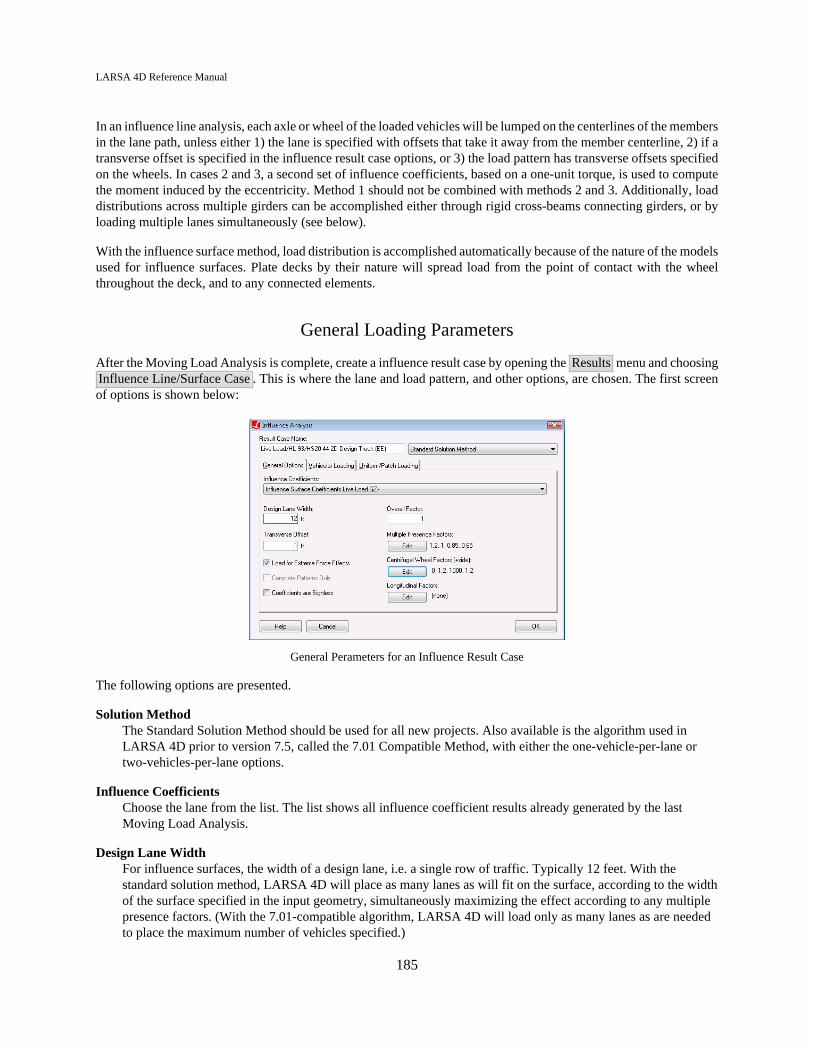
LARSA 4D Reference Manual
In an influence line analysis, each axle or wheel of the loaded vehicles will be lumped on the centerlines of the membersin the lane path, unless either 1) the lane is specified with offsets that take it away from the member centerline, 2) if atransverse offset is specified in the influence result case options, or 3) the load pattern has transverse offsets specifiedon the wheels. In cases 2 and 3, a second set of influence coefficients, based on a one-unit torque, is used to computethe moment induced by the eccentricity. Method 1 should not be combined with methods 2 and 3. Additionally, loaddistributions across multiple girders can be accomplished either through rigid cross-beams connecting girders, or byloading multiple lanes simultaneously (see below).
With the influence surface method, load distribution is accomplished automatically because of the nature of the modelsused for influence surfaces. Plate decks by their nature will spread load from the point of contact with the wheelthroughout the deck, and to any connected elements.
General Loading Parameters
After the Moving Load Analysis is complete, create a influence result case by opening the Results menu and choosingInfluence Line/Surface Case . This is where the lane and load pattern, and other options, are chosen. The first screenof options is shown below:
General Perameters for an Influence Result Case
The following options are presented.
Solution MethodThe Standard Solution Method should be used for all new projects. Also available is the algorithm used inLARSA 4D prior to version 7.5, called the 7.01 Compatible Method, with either the one-vehicle-per-lane ortwo-vehicles-per-lane options.
Influence CoefficientsChoose the lane from the list. The list shows all influence coefficient results already generated by the lastMoving Load Analysis.
Design Lane WidthFor influence surfaces, the width of a design lane, i.e. a single row of traffic. Typically 12 feet. With thestandard solution method, LARSA 4D will place as many lanes as will fit on the surface, according to the widthof the surface specified in the input geometry, simultaneously maximizing the effect according to any multiplepresence factors. (With the 7.01-compatible algorithm, LARSA 4D will load only as many lanes as are neededto place the maximum number of vehicles specified.)
185

LARSA 4D Reference Manual
Transverse OffsetThis option for influence lines simplifies the creation of multiple lanes at different transverse locations. Withthis method, moments on the girder are computed by adding in the effect of special unit-torque influencecoefficients, multiplied by the transverse offset and the axle/wheel magnitude. This method may be more usefulthan adjusting the lane geometry because it eliminates the need to create a separate lane definition (page 83) foreach traffic lane. Only a single lane definition, specified on the centerline of the bridge girder, is necessary tocompute the effects of vehicles on parallel lanes. The sign convention generally follows the right-hand-rule butis truly determined by the orientation of the member elements and the direction of the unit force loading, so it isalways best to verify this by inspection.
Load for Extreme Force EffectsWhen this option is checked, vehicle wheels/axles and lane loading locations that do not contribute to extremeforces are not considered. For example, when enveloping for maximum forces, axles that cause negative forcesare ignored. Normally this option should be on. In LARSA 4D 7.6, this option does not affect lane loadingwhich is always applied in a patch loading manner. In LARSA 4D 7.1, this option must be turned on to applylane loading as patch loading.
Complete Patterns OnlyOften the worst position of a vehicle is when it is only partially on the lane or surface. When this option ischecked, only vehicle positions where all wheels/axles fall on the lane or surface are considered. When nowheel/axle is at the zero-position of the vehicle load pattern, the zero-position must also be on the surface.When this option is not checked, the vehicle may extend past the beginning or end of the line or surface(longitudinally), but for an influence surface vehicles will never extend transversely outside of a design lane,which are always fully contained within the defined surface area.
Overall FactorThe overall factor is applied to the final influence results. Usually this is 1.0.
Multiple Presence FactorsFor influence surfaces, this is a set of factors to apply to the final results depending on the number of lanesactually loaded. The number of lanes loaded will depend on how many lanes fit on the roadway surface andwhether adding additional vehicles can produce a more extreme effect (since more lanes usually means areduced factor). When editing multiple presence factors, enter a table whose first column is the number of lanesloaded and whose second column is the corresponding factor (see below). (With the 7.01-compatible solutionalgorithm, this option applies only to the one- or two-vehicles-per-lane option.)
Multiple Presence Factors
The following advanced options are for modeling centrifugal and braking effects.
Centrifugal Wheel Factors
186

LARSA 4D Reference Manual
For influence surfaces, this option allows the vehicle load pattern to be modified according to a commonfactoring scheme used with centrifugal effects. Load factors are specified to the wheels on the positive-transverse side of the vehicle (always check which way this is by inspection). If the span is curving towardthe positive-transverse direction, the overturning effect will cause vehicle load to shift toward the negative-transverse side. In this case, specify a factor f between zero and one. On the assumption of two wheels per axle,a corresponding factor of 2.0-f will be applied to the wheels on the negative-transverse side of the vehicle (thusresulting in no overall change in applied force). To accommodate multiple spans with different degrees anddirections of curvature, it is possible to specify different factor for different spans. Tbe factor is entered as acurve. The figure below shows how to enter a factor that is constant along the length of a 1000-foot bridgecurving clockwise. (Note that these factors are for vertical loads. For centrifugal force effects, see Guide toAASHTO LRFD 2007 Section 3.6: Live Loads [in LARSA 4D User’s Manual].)
Centrifugal Wheel Factors
Longitudinal FactorsThis option allows an overall factor to be applied that varies longitudinally. It is primarily intended to be usedwhen modeling centrifugal forces on a multi-curve bridge. For an example, see Guide to AASHTO LRFD 2007Section 3.6: Live Loads [in LARSA 4D User’s Manual].
Coefficients are SignlessThis option is used to model braking forces, which can occur in either longitudinal direction if vehicles arepermitted to travel in either direction. When this option is on, each influence coefficient is treated as if it wereits absolute value.
Vehicular Loading Options
The second set of options pertains to vehicular loading. With the standard solution method, vehicular loading may beomitted to apply only uniform lane loading. The options are shown in the following figure and are described below.The figure shows standard options for AASHTO LRFD.
187

LARSA 4D Reference Manual
Combined Cases
The following explanation applies to the standard solution method only.
In the vehicular loading options tab, the user specifies the vehicle type(s) to apply to the structure, and associatedoptions. In the simplest case, a single vehicle type is applied to the structure. However, it is also possible to applydifferent vehicle types in each lane. This is explained later.
Vehicle Load PatternThe load pattern to apply to the structure, from the load patterns in any connected databases (see ConnectingDatabases [in LARSA 4D User’s Manual]). The vehicle load pattern does not include lane loading.
FactorFor each load pattern, a factor may be applied to the magnitudes of the loads. The factor is applied to thevehicle axles only, and not any additional uniform lane loading specified.
To place two vehicles within a design lane, click the Add Vehicle button and then set the load pattern and factor ofthe second vehicle. (By default it will copy the settings of the first vehicle.)
The following options apply to all lane types (explained below):
Min. Back-to-Front SpacingWhen multiple vehicles are placed in the same lane configuration, this is the smallest space allowed betweenthe rear-most axle of one vehicle and the start of another (station zero in the vehicle definition).
Design Lane MarginFor influence surfaces, the margin on each side of design lanes in which vehicle loading is excluded. Thus for a12 foot lane, a 1 foot margin means a possible loading area of 10 feet. This is depicted in the following figure:
188

LARSA 4D Reference Manual
Design Lanes and Vehicle Margin
One Load Pattern Per SpanThe AASHTO LFD design code requires that in certain cases loads be applied only once per span. This optionenforces that constraint. Be sure to add multiple load patterns to the lane configuration and to place spanbreak markers in the lane path definition (page 83). Place span break markers between geometry points that fallon different spans in the structure. Span break markers should be placed in the row immediately followinga geometry point positioned at the end of a span. For instance, if a span ends between members 3 and 4, ageometry point should be created either on member 3 but with an x-offset of end or, as is usually done, onmember 4 but with the default x-offset of start. A span break marker then follows this row. Thus note that aspan break marker usually follows a geometry point on a member that is actually on the next span. Span breakmarkers must be added to the lane definition before the moving load analysis is performed.
Span Break Markers in the Lane Path Definition
The standard solution method supports the notion of a lane type. A lane type is a loading scenario. In AASHTO LRFD,for instance, there are three loading scenarios which can be entered as three lane types: 1) one design truck, 2) twodesign trucks with a factor, and 3) a design tandem. To create additional lane types after the first, click the Add LaneType button and then set the Vehicle Load Pattern and Factor options for each vehicle entered within the new lane type.
The LARSA 4D influence vehicle loading algorithm will choose the lane type for each design lane that causes themost extreme effect. Each design lane may be assigned a different lane type.
Each lane type has two additional options:
Max Lanes
189
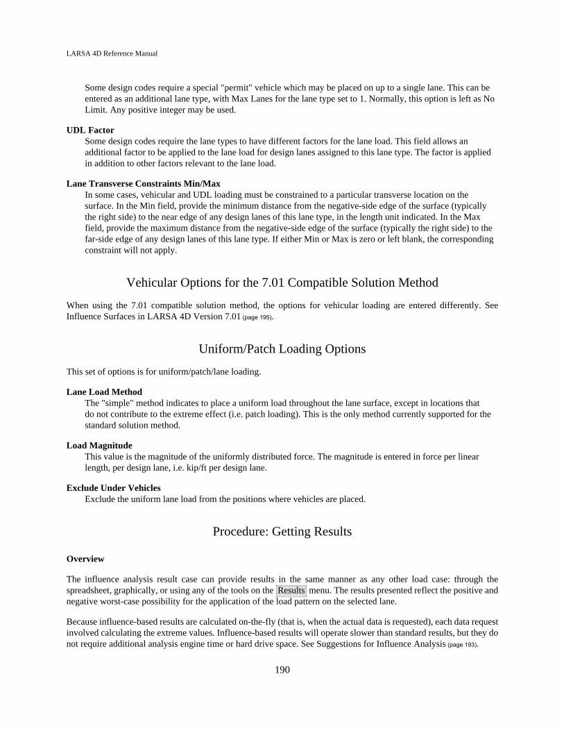
LARSA 4D Reference Manual
Some design codes require a special "permit" vehicle which may be placed on up to a single lane. This can beentered as an additional lane type, with Max Lanes for the lane type set to 1. Normally, this option is left as NoLimit. Any positive integer may be used.
UDL FactorSome design codes require the lane types to have different factors for the lane load. This field allows anadditional factor to be applied to the lane load for design lanes assigned to this lane type. The factor is appliedin addition to other factors relevant to the lane load.
Lane Transverse Constraints Min/MaxIn some cases, vehicular and UDL loading must be constrained to a particular transverse location on thesurface. In the Min field, provide the minimum distance from the negative-side edge of the surface (typicallythe right side) to the near edge of any design lanes of this lane type, in the length unit indicated. In the Maxfield, provide the maximum distance from the negative-side edge of the surface (typically the right side) to thefar-side edge of any design lanes of this lane type. If either Min or Max is zero or left blank, the correspondingconstraint will not apply.
Vehicular Options for the 7.01 Compatible Solution Method
When using the 7.01 compatible solution method, the options for vehicular loading are entered differently. SeeInfluence Surfaces in LARSA 4D Version 7.01 (page 195).
Uniform/Patch Loading Options
This set of options is for uniform/patch/lane loading.
Lane Load MethodThe "simple" method indicates to place a uniform load throughout the lane surface, except in locations thatdo not contribute to the extreme effect (i.e. patch loading). This is the only method currently supported for thestandard solution method.
Load MagnitudeThis value is the magnitude of the uniformly distributed force. The magnitude is entered in force per linearlength, per design lane, i.e. kip/ft per design lane.
Exclude Under VehiclesExclude the uniform lane load from the positions where vehicles are placed.
Procedure: Getting Results
Overview
The influence analysis result case can provide results in the same manner as any other load case: through thespreadsheet, graphically, or using any of the tools on the Results menu. The results presented reflect the positive andnegative worst-case possibility for the application of the load pattern on the selected lane.
Because influence-based results are calculated on-the-fly (that is, when the actual data is requested), each data requestinvolved calculating the extreme values. Influence-based results will operate slower than standard results, but they donot require additional analysis engine time or hard drive space. See Suggestions for Influence Analysis (page 193).
190

LARSA 4D Reference Manual
Envelopes
Because influence-based results search for a minimum and maximum, LARSA 4D must know which column from aresult spreadsheet to envelope on. If LARSA 4D is enveloping on the member's z-moment, the member's correspondingy-moment will not be the minimum/maximum y-moment but instead will be the y-moment produced from the sameaxle positions that produced the greatest z-moment. In this way, an entire row of a spreadsheet comes from the sameaxle positions. You must use envelopes to view influence-based results so that LARSA 4D knows which value toenvelope on.
Not all graphical results use envelopes automatically. The other results, such as member forces and stresses,automatically envelope on the result column being displayed. If axial force is being shown graphically, then theinfluence results will envelope on axial force.
Special Graphical Results Tools
A special influence coefficients graphical view [see “Influence Coefficients Graphical View” in LARSA 4D User’sManual] is available, showing the influence coefficients as well as computed truck axle positions.
Special Spreadsheet Results Features
In results spreadsheets, the Result Case column of influence-based results indicates the specific loading configurationthat yielded the extreme result of each row.
The cell value lists the coordinate of each placed vehicle in the form of “s4./t35.25”, for example, which means thehead of the vehicle is 4 coordinate units from the start of the surface (“s” stands for “station”) and at a transverselocation of 35.25 coordinate units (where zero is at the centerline of the surface and sign follows the right hand rule).The head of the vehicle is the (0,0) coordinate in the load pattern definition, which is typically at the location of thefront wheels on the centerline of the vehicle.
If the configuration text is followed by “UDL”, it indicates that uniform lane loading was applied.
If the configuration text is followed by “* 1.2 (mp)”, a multiple presence factor (such as 1.2) was applied.
If the configuration text is followed by “* .9”, it indicates an overall factor was applied.
For More Information, please refer to the following documentation.
• Lanes on page 83.
• Influence Loads on page 109.
• Moving Load Analysis on page 179.
191

LARSA 4D Reference Manual
192

LARSA 4D Reference Manual
Suggestions for Influence Analysis
This section provides some suggestions for running influence analysis.
Suggestions for Speed
Because of the large number of computations involved in influence analysis, speed can be a concern.
Using Larger IncrementsTry increasing the forward and transverse increments in the influence coefficients load case. With fewercoefficients generated, there are fewer results to scan through to optimize vehicle and UDL positions.
Cache Results ( Tools # Options # General Options )As influence based results are requested, the computed results are saved into a cache file. This way, thenext time same influence result is requested, it can be retrieved from the cache quickly. Optimizationoccurs as user requests data.
Pre-cache Results ( Results # Pre-cache Results )You may want to use this tool before the leaving office so that it works during the night. The next day youcan access all influence results just like static runs.
I/O Optimization ( Results # I/O Optimization )The first time LARSA tries to access a result file, the complete file will be loaded into system memory(assuming enough memory exist on the system). This way repeated disk access is avoided. The files areloaded into the memory as they are requested. This feature only loads original analysis engine generatedresult files, not the files generated by the above methods.
193

LARSA 4D Reference Manual
194

LARSA 4D Reference Manual
Influence Surfaces in LARSA 4D Version 7.01
This section describes options of an earlier version of LARSA 4D.
Design Lane Options
Since version 7.01, LARSA 4D can automatically determine the placement of design lanes on a roadway surface.Before this version, lane definitions were considered design lanes, and loading was applied accordingly. Since version7.01, lane definitions can represent roadway surfaces, and the locations of design lanes will be found automatically.In the 7.01 solution method there are three options for loading placement for influence surfaces which are chosen inthe influence loading setup window:
Place Vehicles Anywhere
The lane definition is taken as a single design lane, with vehicles allowed to be placed anywhere on the lane.UDL lane loading is applied across the entire width of the lane. (This was the method always in effect beforeLARSA 4D version 7.01.) With this option, you may need to create multiple lane definitions and mutlipleinfluence cases to cover the different scenarios of live loads.
Place Vehicles Anywhere Option: The "lane" definition represents a single design lane.
One Vehicle Per Lane
The lane definition is considered a roadway surface, and the user must additionally specify the Design LaneWidth and Design Lane Margin . With this option, trucks are loaded subject to a lane placement constraint.Only as many trucks listed in the Max # field will be placed, so the user must be sure to specify a number atleast as large as the potential number of lanes that may fit on the roadway surface.
The lane placement constraint is that each vehicle must fall entirely within its own design lane, whose widthis given as Design Lane Width, and cannot fall in a margin on each side of the lane (specified as the DesignLane Margin, meaning the width on either side of the lane that loading is excluded from), and of courselanes cannot overlap.
Any UDL lane load specified is applied only on the portion of the roadway surface that design lanes wereplaced at, excluding design lane margins. The UDL magnitude is applied per design lane, which means thatunlike with the previous option, the magnitude of the UDL per liner foot across the entire roadway surfacewill depend on the number of design lanes automatically placed.
195
LARSA 4D Reference Manual
One Vehicle Per Lane: The "lane" definition represents a roadway surface. Designlanes are placed automatically on the surface, with one vehicle per design lane.
Two Vehicles Per Lane
This option works similarly as with One Vehicle Per Lane, except that at most two vehicles are placed ineach lane. As above, only as many trucks listed in the Max # field will be placed, so the user must be sureto specify a number at least twice the potential number of lanes that may fit on the roadway surface. Theplacement of the second truck on any lane is constrained to be at the same transverse offset as the first truck.
Vehicle Type and Placement Options
Enter the total set of vehicles to be applied to the structure. Note that while in the standard solution method each typeof vehicle is entered once, with the 7.01 compatible solution method a vehicle must be entered for as many times asit could be applied to the structure. On a three-lane span, the vehicle must be entered either three times or once butwith the Max # field set to 3.
The UDL factor is not applicable. The design lane vehicle margin option is applicable with the one- or two-vehicles-per-design-lane option. The following additional option is available:
Min. Side-to-Side SpacingFor influence surfaces only, the smallest space allowed between the sides of two nearby vehicles, as determinedby the (transverse) distance from the centerline of the leftmost load of one vehicle to the centerline of therightmost load of another.
The one vehicle per span option has a different meaning with this solution method. See AASHTO LFD Point Loadingin LARSA 4D Version 7.01 (page 197).
196

LARSA 4D Reference Manual
AASHTO LFD Point Loading in LARSA 4DVersion 7.01
This section describes options for a previous version of LARSA 4D.
The AASHTO LFD Point Loading option adds extra processing to the influence case for use with the AAHSTO LFDprovision that when applying point loads to determine negative moments, a second point load of equal magnitude isto be placed on a different span from the first point load.
To use this option, span break markers must be added to the lane path definition (page 83). Place span break markersbetween geometry points that fall on different spans in the structure. Span break markers should be placed in the rowimmediately following a geometry point positioned at the end of a span. For instance, if a span ends between members3 and 4, a geometry point should be created either on member 3 but with an x-offset of end or, as is usually done, onmember 4 but with the default x-offset of start. A span break marker then follows this row. Thus note that a span breakmarker usually follows a geometry point on a member that is actually on the next span. Span break markers must beadded to the lane definition before the moving load analysis is performed.
Span Break Markers in the Lane Path Definition
Then set up an influence case with two single-point-load load patterns and check the AASHTO LFD Point Loadingoption, as shown in the figure below.
AASHTO LFD Point Loading Option
197

LARSA 4D Reference Manual
Results produced by this case will reflect the application the first point load always, and in addition the second pointload when negative moments in Member End Forces or Member Sectional Forces are being viewed.
Here, 'negative moments' is taken the mean the moments at the top of horizontal members, with the global-z axis being'up'. For any given member, negative moments are applicable to either the Moment Y or Moment Z column, and eitherthe envelope minimums or the envelope maximums. Which column and extreme is used depends on the orientation ofthe member and the sign convention of the result type, according to the following table:Member Orientation Orientation Angle Negative
Moments Are...Sign Used forEnd Forces
Sign Used forSectional Forces
Local-Y is Up 90 (or close to 90) Moment Z Maximums at Start,Minimums at End
Minimums
Local-Y is Down 270 Moment Z Minimums at Start,Maximums at End
Minimums
Local-Z is Up 0 Moment Y Minimums at Start,Maximums at End
Maximums
Local-Z is Down 180 Moment Y Maximums at Start,Minimums at End
Maximums
198

LARSA 4D Reference Manual
Standard Vehicles
Various standard vehicle types are supplied with LARSA 4D. These vehicles include AASHTO (American Associationof State Highway and Transportation Officials) trucks, AASHTO alternate military loads, CALTRANS P type permitloads and Indian Roads Congress vehicles.
AASHTO and CALTRANS Vehicles
The AASTHO H loadings consist of a two-axle truck, the HS loadings consist of a tractor with semi-trailers, andCALTRANS P loadings are special vehicular loads. These loads are found in the file movedata.dml .
The patterns are one dimensional: Axles are point loads applied to the center-line of lanes.
• HS20-44 is an AASHTO HS truck consisting of a tractor truck with a semi-trailer. The total weight is 72kips.
• HS15-44 is an AASHTO HS truck with 75 percent loading of HS20.
• H20-44 is an AASHTO H truck consisting of a two-axle truck. The total weight is 40 kips.
• H15-44 is the Standard H truck with 75 percent loading of H20.
• H20-S16-T16 consists of five axles with total weight of 104 kips.
• HN-72 is a highway normal truck with total weight of 54 kips.
• HO-72 is a highway overweight truck with total weight of 108 kips.
• LEGAL-TYPE3 is an AASHTO Legal Load Type 3 with three axles and the total weight is 50 kips.
• LEGAL-TYPE3S2 is an AASHTO Legal Load Type 3S2 with five axles and the total weight is 72 kips.Input Data Description 9-137
• LEGAL-TYPE3-3 is an AASHTO Legal Load Type 3-3 with six axles and the total weight is 80 kips.
• P5, P7, P9, P11 and P13 are CALTRANS-P loads (permit design live loads). The distance between each axleis 18 feet. The first axle is 26 kips and the remaining axles are 48 kips. The vehicles have 3, 4, 5, 6, and 7axles, respectively.
AASHTO Load Patterns for Influence Analysis
These load patterns are provided primarily for use in influence-based analysis following the AASHTO LRFD designcode for live load analysis. Some are defined with variable axle spacing, which only applies in that type of analysis.These patterns are found in the files movedata.dml or AASHTO Vehicle Patterns.dml .
Some of these patterns are two dimensional. 2D load patterns can only be used with influence-based analysis.
• HL-93/HS20-44 Design Truck has three axles of 8, 32, and 32 kips. The spacing between the front two axlesis 14 feet, and in influence-based analysis the spacing between the rear axles varies between 14 and 30 feet.This load pattern does not specify a width for the vehicle, so should not be used in influence surface analysiswithout noting the implications for vehicle placement and the side-to-side spacing option.
• HL-93 Design Tandem consists of two 25 kip loads spaced 4 feet apart. This load pattern does not specify awidth for the vehicle, so should not be used in influence surface analysis without noting the implications forvehicle placement and the side-to-side spacing option.
199

LARSA 4D Reference Manual
• HL-93/HS20-44 2D Design Truck has six wheels, modeled as point loads offset 3 feet each way from thevehicle center. It has the same spacing, including variable axle spacing, as the one-dimensional HL-93pattern above, except that the axles are split into pairs of wheels.
• AASHTO Point 18 kip moment/26 kip shear/13.5 kip moment/19.5 kip shear are point load patterns with thegiven type and magnitude. They are provided for using the influence-based analysis with span loading in theAASHTO code.
There are two vehicle load patterns that model tire contact area with distributed loads. Tire contact area is specified asuniformly distributed loads over a rectangular surface at the appropriate transverse coordinates.
• HL-93 Design Truck T/C is similar to the HL-93 Design Truck, except that tire contact area is moreprecisely modeled by specifying two tires per axle at the appropriate transverse positions, and by includingtransverse width and tire length. This pattern does not include variable axle spacing, however, and tirecontact area rarely plays a role, so the HL-93/HS20-44 2D Design Truck Pattern is recommended to be usedin place of this pattern.
• HL-93 Design Tandem T/C or HL-93 Design Tandem 2D is similar to the HL-93 Design Tandem, except ithas four loads, two for the front axle and two for the back, each 12.5 kips distributed over a 10x20 inch area.The tires are laterally offset from the center-line by 3 feet.
Other load patterns are available but are no longer recommended for use:
• HL-93 Design Two Trucks consists of two HL-93 design trucks at variable spacing, but each truck havingfixed axle spacing at 14'. The use of this load pattern is deprecated in favor of using the number of vehiclesto load and minimum vehicle spacing options of the influence-based analysis.
IRC Load Patterns for Influence Analysis
These load patterns are provided primarily for use in influence-based analysis following the Indian Roads Congressdesign code for live load analysis. These patterns are found in the file IRC Load Patterns.dml .
These patterns are all two dimensional: Rather than specifying axles, the actual wheels of the load patterns are specified(generally two per axle) at the appropriate transverse position. In patterns marked "Distributed," tire contact areais specified as uniformly distributed loads over a rectangular surface. Those not marked "Distributed" have wheelsmodeled as point loads. Distributed patterns are provided for the influence surface analysis.
When used in the standard moving load analysis, transverse positions of wheels are ignored. All wheels are lumpedon the center-line of the lane.
• IRC Class AA Tracked is the Class AA tracked tank pattern, comprising two 350 kN distributed loads 3.6meters long and .85 meters wide, offset by 1 meter in each direction from the lane center-line.
• IRC Class AA Wheeled is the Class AA wheeled tank pattern, comprising two axles with four wheels peraxle of 37.5 and 62.5 kN.
• IRC Class 70R Tracked is the Class 70R tracked tank similar to the Class AA tracked tank but with a lengthof 4.57 meters.
• IRC Class 70R Load Train is the 7-axle train with load intensities of 40, 60, and 85 kN per wheel (twowheels per axle).
• IRC Class 70R Bogie is the bogie pattern with two axles comprising four wheels of 100 kN each.
• IRC Class A Train is the 8-axle train with load intensities of 13.5, 57, and 34 kN per wheel (two wheels peraxle).
200

LARSA 4D Reference Manual
• IRC Class B Train is the 8-axle train with load intensities of 8, 34, and 20.5 kN per wheel (two wheels peraxle).
For More Information, please refer to the following documentation.
• Moving Load Analysis on page 179.
201

LARSA 4D Reference Manual
202
LARSA 4D Reference Manual
Moving Load Analysis Options
Solution convergence options (Nonlinear Static Analysis Options (page 149)) apply only to the Nonlinear/Linear and FullNonlinear moving load analysis types.
For More Information, please refer to the following documentation.
• Running an Analysis in LARSA 4D User’s Manual.
• Moving Load Analysis on page 179.
203

LARSA 4D Reference Manual
204

LARSA 4D Reference Manual
Staged Construction Analysis
Staged Construction Analysis analyzes a series of construction steps, which represent the steps in the evolution of astructure's construction, demolition, or rehabilitation. The Staged Construction Analysis is a form of nonlinear staticanalysis (page 141) that retains the state of the structure from step to step, automatically applying construction activitiesspecified by the user. Staged Construction Analysis makes scenario testing an automated process.
Overview of Staged Construction Analysis 207
Staged Construction Activities 209
Setting Up the Model 211Preparation 211
Creating Activities in the Explorer 212
Creating Activities in the Stage Editor 213
Time Effects on Materials 217Definitions 217
General Options 218
Load Class Tracking 221Setting up the model 221
The Load Classes of Result Cases 221
Accessing Class-Based Results 222
Staged Construction Analysis Options 223Options for Analysis Scenarios 224
205

LARSA 4D Reference Manual
206

LARSA 4D Reference Manual
Overview of Staged Construction Analysis
Changes to a structure over time are defined in a series of construction steps. Construction steps can includeconstruction activities, such as constructing parts of the structure, applying loads, and modifying support conditions.Time-effects on material behavior, including the effect of super-imposed loads, can be automatically accounted for.
Because the Staged Construction Analysis is a nonlinear analysis, geometric nonlinearity is included, a necessaryfeature for any structure with nonlinear elements, such as cables.
Staged Construction Analysis comes in two types. In the Standard type, a Nonlinear Static Analysis (page 141) isperformed for each construction step, retaining the deformed properties of the structure from step to step. Time-effectson materials are ignored. In the Time-Dependent type, the same nonlinear analysis is performed, but time-effects onmaterials are included.
Elements are activated and deactivated through their inclusion in construction activities. When a Staged ConstructionAnalysis begins, LARSA assumes no elements have been activated. Only elements explicitly constructed inconstruction activities contribute to the stiffness of the structure. If the structure is to start off constructed, the firstconstruction activity should assemble the structure into its constructed state.
A structure can change over time any number of ways in the real world. LARSA supports the following constructionactivities:
• Construction: Parts to the structure are added (assembled). Joint locations can be automatically adjusted basedon the deformed shape of the structure according to contruction methods, a necessary tool for segmental projectssuch as balanced cantilever bridges.
• Deconstruction: Parts of the structure are removed (disassembled).
• Weight and Stiffness: Self-weight and stiffness can be activated in different steps.
• Supports: Joints are restrained or released (globally or slaved to other joints).
• Loads: Loads are applied or removed.
• Tendons: Stressed or slackened.
• Materials: Creep and shrinkage for concrete, and relaxation for steel.
Staged construction often comes hand-in-hand with pre- and post-tensioning elements. Such tensioning is generallyaccomplished with tendons, which are discussed in the tendons section in the Model Data Reference (page 75).
207

LARSA 4D Reference Manual
208

LARSA 4D Reference Manual
Staged Construction Activities
LARSA is able to model continuous changes to a structure over time involving a useful set of construction activities.
Construction activities are specified in two ways, using the Construction Stages Explorer or the Construction StagesEditor. See Setting Up the Model (page 211).
LARSA arranges construction activities into stages and steps.
StagesA stage represents one day of construction, which can consist of one or more steps. Stages are labeled witha day number, a temperature and a humidity value, which apply to all steps within the stage. The day of thestage is used for computing time-effects on materials.
StepsA step represents one set of construction activities to accomplish a goal. Steps occur within stages. Allconstruction activities occur within steps.
Both stages and steps can be given descriptive names.
The construction activities that can be placed within steps are given below. They are described in more detail inConstruction Activities (page 113).
Construction/Deconstruction
Structural elements are at any point constructed or unconstructed. Constructed elements are used in theanalysis of the structure, while unconstructed elements are ignored. Elements start off unconstructed untilthey are explicitly constructed in a step.
To construct or deconstruct (page 115) a part of the model, form a structure group [see “Structure GroupsExplorer” in LARSA 4D User’s Manual] and then drag that group from the Structure Groups Explorer into theConstruction Stages Explorer [in LARSA 4D User’s Manual]. The elements in that group will be constructed.To deconstruct those elements, right-click the stage, choose Properties, and mark the Deconstruct option.
Elements may be constructed in locations relative to the deformed state of the structure. The segmentalconstruction methods (page 115) and joint displacement initialization (below) are used to specify such behavior.Normally, elements are constructed in the position that they are initially defined in.
See Construct and Deconstruct Activities (page 115).
Support Change and Hoist Activitiy
A support's properties have changed, or a joint is becoming a support. Support activities (page 121) specify thenew restraints of a joint (page 47) in all six degrees of freedom.
See Support and Hoist Activities (page 121).
Slave/Master Change
A joint (page 47)'s slave/master (page 73) connectivity is changed. Slave/Master activities specify the new slave/master connections of a joint. Old slave/master connections in all degrees of freedom are discarded for ajoint whenever a new slave/master activity for that joint is encountered.
209

LARSA 4D Reference Manual
See Slave/Master Change Activities (page 123).
Load Application
A static load case (page 91) is applied to the structure. Loads are applied cumulatively; that is, a load appliedin one stage will automatically continue to be applied in all future stages. To "turn off" a load, apply theload again with a negative load factor.
Tendon Application
A tendon (page 75) is stressed or slackened.
See Tendon Stressing and Slackening Activities (page 125).
Displacement Initialization
Alters the initial location of a joint. Normally, when joints are activated they enter at the location that wasinitially given to them. Joints sometimes need to become active in a location relative to the deformed structureof the model, rather than in an exact position known ahead of time. Displacement Initializations specify howto place a joint relative to the deformed location of other joints..
See Displacement Initializations (page 127).
210

LARSA 4D Reference Manual
Setting Up the Model
Construction activities are specified in two ways, using the Construction Stages Explorer or the Construction StagesEditor. This section explains how to use each method.
Structural changes occur in a serial or linear fashion. An example of staged construction might be . . .
1. Construct Left Pier
2. Construct Right Pier
3. Construct Center Temporary Pier (modeled as fixing center joint in space)
4. Construct Span from Left to Temporary Pier
5. Construct Span from Right to Temporary Pier
6. Stress Tendons
7. Deconstruct Temporary Pier (modeled as releasing center joint)
Each of those steps is refered to as a construction activity.
Preparation
Before defining construction activities in LARSA,
1. All elements in the structure that will ever be assembled must be modeled.
Structures should be modeled as if every member, plate, and spring used at any point during construction areall present at the same time. The time at which elements are constructed will be specified later.
As a result, all joints that will ever be a part of the model must be in the project. Joints are automaticallyincluded in the model when elements attached to it become constructed and are automatically removed fromthe model when all attached elements are deconstructed.
Tendons (page 75) and other structural objects must also be entered before proceeding on to modelingconstruction activities.
2. Restraints must be set to initial conditions
Joints will be initially restrained as their restraints are specified in the project, taking into account standardrestraints (page 47) and slave/masters (page 73).
3. Groups of elements that will be constructed or deconstructed together should be put into structure groups[see “Structure Groups Explorer” in LARSA 4D User’s Manual].
Although structure groups need not be defined ahead of time, it will save time later.
The steps outlined from this point on assume that the above tasks have been completed.
211

LARSA 4D Reference Manual
Creating Activities in the Explorer
Construction Stages Explorer
The Construction Stages Explorer presents the construction stages and steps in the same style as the example above.A screenshot is on the right.
For more information on the meaning of each type of construction activity, see Staged Construction Activities (page 209).
Using the Explorer:
• To open the Explorer if it is not already open, right click the title bar area of the open Explorer (where it reads"Construction Stages" in the figure) and choose Construction Stages.
• To add a construction stage, click the Add Stage button, which looks like a folder. A new stage will be addedto the bottom of the list of stages. Each stage is labeled with the day on which its steps' activity occurs, whichis "day 0" by default.
• To add a construction step to the project, select the stage in which to add the new step, and then click theAdd Step button, which looks like a small frame.
• To delete a stage or step, select the stage or step and then click the Delete button, which looks like an X.
• To rename a stage or a step, select the stage or step, and then hit F2 . Type the new name, and then hit Enter .
• If after adding various stages they have become out of chronological order, click the Sort button. The stageswill be sorted by Day.
Preparing for Time Effects in the Explorer:
• To include time-effects on materials in construction analysis, each construction stage must have a timeassigned, determined by a stage's Day. To edit a stage's day, select the stage. Then, make the change in the textbox at the bottom of the explorer. Hit the checkmark to finalize the change.
• To modify the humidity or temperature of a stage, which is used to compute time-effects on materials inconstruction analysis, open the Load Groups & Stages spreadsheet window, which can be found in the InputData menu. Select the Construction Stages tab. This spreadsheet will show a list of the stages added to theproject, but not the construction steps.
Adding Construction Activities in the Explorer:
212

LARSA 4D Reference Manual
• If part of the structure is to be constructed or deconstructed in a step, click and drag a Structure Group[see “Structure Groups Explorer” in LARSA 4D User’s Manual] of those elements from the Structure GroupsExplorer onto the step in the Construction Stages Explorer during which they will be constructed.
To see the two Explorers at once, double-click the title bar area of the open Explorer (where it reads"Construction Stages" in the figure). The right click the title area of the Explorer on the bottom and chooseStructure Groups. Double click the title area of the top Explorer again to close the lower Explorer.
Structure groups in a step must be either all constructed or all deconstructed. Use multiple steps if bothconstruction and deconstruction will occur.
If that structure group is to be deconstructed, right-click the construction step (not the group). Click Propertiesand choose the Deconstruct option. The step will become a deconstruction step, indicated by a red X throughthe step's icon.
Structure groups can be constructed in weight-only mode in which the self-weight of the group is applied tothe structure but the group adds no stiffness to the structure. This is useful when a concrete member is pouredbut not immediately hardened. To specify that a structure group be weight-only, right click the group and selectWeight Only. To have the group contribute stiffness in a later stage, add the group to the Construction StagesExplorer again, but without the weight-only option.
• Static load cases are be applied during a step by dragging a load case from the Load Cases Explorer [see “LoadCases Explorer” in LARSA 4D User’s Manual] onto the step in the Construction Stages Explorer during whichthe load case should be applied. To see the two Explorers at once, see the previous point.
• Other activities are accessed
• Using the Construction Stage Editor, which is explained below, or
• Through spreadsheets [see “Using the Model Spreadsheets” in LARSA 4D User’s Manual]. To add theseactivities to a step, right-click the step and then select Support, Slave, Tendon Activity .
Creating Activities in the Stage Editor
The construction stage editor is an alternative way of building/editing the stage construction data in LARSA 4D. Unlikethe Construction Stages Explorer, the Construction Stage Editor uses a spreadsheet based approach to orginize the data.
The spreadsheet does not only contains the data but also some commands with a self explanatory label to theirfunctionality. These commands can be easily distinguised by their red, italic, underlined format. Double clicking onthese commands will activate them.
Each spreadsheet contains the commands to add, remove, and rename stages and steps.
The dialog box is composed of six tab menus. Each menu represents a type of spreadsheet. Below you find theexplanation on each tab menu and how it is being used.
For more information on the meaning of each type of construction activity, see Staged Construction Activities (page 209).
On the Stage/Steps spreadsheet, you can:
• Add, remove, and rename stages and steps,
• Specify whether each step is for construction or deconstruction, and
• Define the segmental construction method (page 115) of each step. Unless your model needs to update jointlocations to account for deformation, the Standard method should be chosen.
213
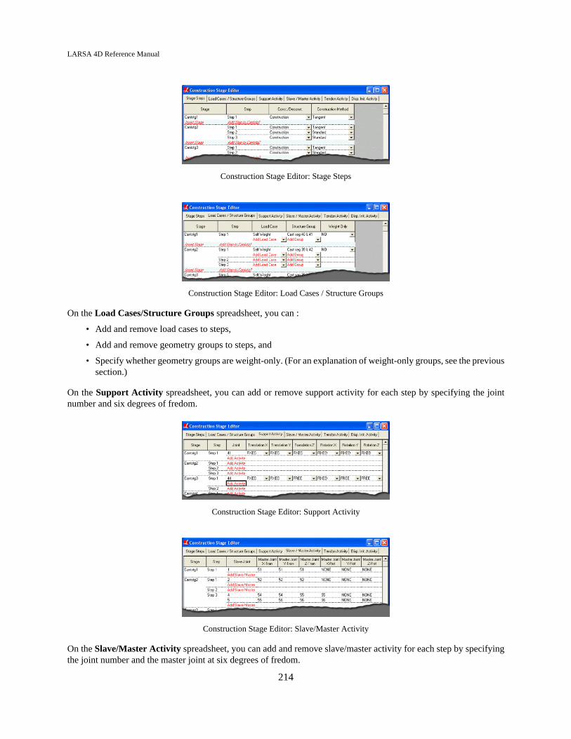
LARSA 4D Reference Manual
Construction Stage Editor: Stage Steps
Construction Stage Editor: Load Cases / Structure Groups
On the Load Cases/Structure Groups spreadsheet, you can :
• Add and remove load cases to steps,
• Add and remove geometry groups to steps, and
• Specify whether geometry groups are weight-only. (For an explanation of weight-only groups, see the previoussection.)
On the Support Activity spreadsheet, you can add or remove support activity for each step by specifying the jointnumber and six degrees of fredom.
Construction Stage Editor: Support Activity
Construction Stage Editor: Slave/Master Activity
On the Slave/Master Activity spreadsheet, you can add and remove slave/master activity for each step by specifyingthe joint number and the master joint at six degrees of fredom.
214

LARSA 4D Reference Manual
On the Tendon Activity spreadsheet, you can
• Add and remove tendon activity for each step, and
• Specify whether each tendon is stressed or slackened.
Construction Stage Editor: Tendon Activity
Construction Stage Editor: Displacement Initialization Activity
On the Displacement Initialization Activity spreadsheet, you can add and remove displacement initializationactivities for each step by specifying the joint number that the initialization process will take place, the joints at bothends, and the adjustment direction.
215

LARSA 4D Reference Manual
216

LARSA 4D Reference Manual
Time Effects on Materials
Time effects on materials account for concrete creep and shrinkage, steel creep and relaxation, and other materialchanges.
Conventional analyses do not account for materials whose properties change over time. Concrete is subject to creepand shrinkage. Steel is subject to relaxation, and in fire it is subject to creep as well. These changes and elastic modulusvariation are accounted for in LARSA's time-dependent staged construction analysis.
Time-dependent deformation of concrete resulting from creep and shrinkage is of crucial importance in the design ofprestressed concrete structures because these changes result in a partial loss of prestress force with significant changesin deflections.
Concrete creep and shrinkage, tendon relaxation, the time-effect on elastic modulus are based on the prediction modelsand equations from FIP-CEB90 and FIP-CEB78, AASHTO, ACI, BS5400-4, BS8110-2 codes or user-defined materialproperty curves for time-dependent behavior.
Time-Dependent Stage Construction Analysis also requires time, temperature, and humidity conditions at each stage.
Definitions
The following time-dependent material effects can be computed by LARSA. Which effects to include are specifiedin options, which are explained below.
Concrete CreepCreep is the property of many materials by which they continue deforming over considerable lengthsof time at constant stress or load. Creep strain for concrete depends not only time, but on the mixproportions, humidity, curing conditions and the age of concrete when it is first loaded. The rate of strainincrease is rapid at first, but decreases with time until a constant value is approached asymptotically. InLARSA 4D, creep is available for member elements and includes creep due to axial force and the twobending moments.
Concrete ShrinkageNormal concrete mixes contain more water than is required for hydration of the cement where the freewater evaporates in time. Drying of concrete is accompanied by a reduction in volume. The rate of dryingdepends on the humidity, ambient temperature, and the size and shape of the concrete element and thechange in volume occurs at a higher rate initially.
Steel Relaxation
When prestressing steel is stressed to the levels that are customary during initial tensioning and at serviceloads, it exhibits a property known as relaxation. Relaxation is defined as the loss of stress in a stressedmaterial held at a constant length. This same phenomenon is known as creep when defined in terms of changein length of a material under constant stress. In prestressed concrete members, creep and shrinkage of theconcrete as well as fluctuations in superimposed loads cause change in tendon length. Relaxation is not ashort-lived phenomenon, it continues almost indefinitely, although at a diminishing rate.
Relaxation must accurately be accounted for in the design because it produces significant loss of prestressforce. The amount of relaxation varies depending on the type and grade of steel, but most significantparameters are time and intensity of the initial stress.
217
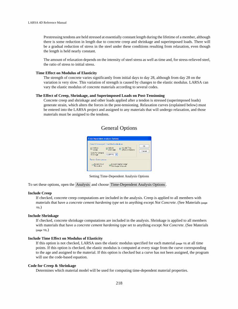
LARSA 4D Reference Manual
Prestressing tendons are held stressed at essentially constant length during the lifetime of a member, althoughthere is some reduction in length due to concrete creep and shrinkage and superimposed loads. There willbe a gradual reduction of stress in the steel under these conditions resulting from relaxation, even thoughthe length is held nearly constant.
The amount of relaxation depends on the intensity of steel stress as well as time and, for stress-relieved steel,the ratio of stress to initial stress.
Time Effect on Modulus of ElasticityThe strength of concrete varies significantly from initial days to day 28, although from day 28 on thevariation is very slow. This variation of strength is caused by changes to the elastic modulus. LARSA canvary the elastic modulus of concrete materials according to several codes.
The Effect of Creep, Shrinkage, and Superimposed Loads on Post-TensioningConcrete creep and shrinkage and other loads applied after a tendon is stressed (superimposed loads)generate strain, which alters the forces in the post-tensioning. Relaxation curves (explained below) mustbe entered into the LARSA project and assigned to any materials that will undergo relaxation, and thosematerials must be assigned to the tendons.
General Options
Setting Time-Dependent Analysis Options
To set these options, open the Analysis and choose Time-Dependent Analysis Options .
Include CreepIf checked, concrete creep computations are included in the analysis. Creep is applied to all members withmaterials that have a concrete cement hardening type set to anything except Not Concrete. (See Materials (page
19).)
Include ShrinkageIf checked, concrete shrinkage computations are included in the analysis. Shrinkage is applied to all memberswith materials that have a concrete cement hardening type set to anything except Not Concrete. (See Materials(page 19).)
Include Time Effect on Modulus of ElasticityIf this option is not checked, LARSA uses the elastic modulus specified for each material (page 19) at all timepoints. If this option is checked, the elastic modulus is computed at every stage from the curve correspondingto the age and assigned to the material. If this option is checked but a curve has not been assigned, the programwill use the code-based equation.
Code for Creep & ShrinkageDetermines which material model will be used for computing time-dependent material properties.
218

LARSA 4D Reference Manual
CEBFIP78This code uses a user-defined material model based on the CEBFIP78 guidelines. Use this option tosupply custom curves for special environmental conditions. This code requires the following time-dependent material curves (page 41) to be entered by the user:
• Concrete Shrinkage Curve
• Concrete Delayed Plastic Strain Curve
• Concrete Delayed Elastic Strain Curve
• Stress/GUTS vs. Relaxation Curve
• Time vs. Relaxation Curve
• Time versus Elastic Modulus Curve.
CEBFIP90This code requires the following time-dependent material curves (page 41) to be entered by the user:
• Stress/GUTS vs. Relaxation Curve
• Time vs. Relaxation Curve
This code has built-in equations for the computation of creep and shrinkage coefficients and therefore doesnot require the following curves to be entered by the user.
• Concrete Shrinkage Curve
• Concrete Delayed Plastic Strain Curve
• Concrete Delayed Elastic Strain Curve
• Time versus Elastic Modulus Curve
Include Steel RelaxationWhen this option is checked, prestressing losses in tendons from steel relaxation are included. Relaxationcurves (explained above) must be entered into the project and assigned to any material that will undergorelaxation, and those materials must be assigned to the tendons.
Losses due to Creep/Shrinkage/SI LoadsIn addition, reduction in prestressing will be computed from the effects of concrete creep and shrinkage, othertendon activity and other loads applied after the tendon is stressed (superimposed loads).
219

LARSA 4D Reference Manual
220

LARSA 4D Reference Manual
Load Class Tracking
Code compliance requires creating factored load combinations, with different factors applied to different classes ofloading, such as dead load, live load, creep, and shrinkage. The Staged Construction Analysis of LARSA 4D reportscumulative effects after each construction step, but it is also possible to extract the partial effects of each load class.Starting with 7.01.60, the partial class-based effects of support, slave/master, and element deconstruction activities arenow available, and these are crucial for creating code-based load combinations in a Staged Construction Analysis.
We discuss below setting up a model for tracking class-based loading in Staged Construction Analysis and how thismethod applies to support changes and element deconstruction.
Setting up the model
In a Staged Construction Analysis model that will use class-based load tracking, it is necessary to ensure that eachload case is assigned a load class. Load classes can be chosen from a pre-set list of 45 classes including "Dead Load","Live Load", "Creep", "Snow Load", and "Prestress". The choice of class does not impact the analysis and is usedonly for reporting partial effects during post-processing. To choose a load class for a load case, use the Load Cases& Combinations Spreadsheet or the Load Cases Explorer [see “Load Cases Explorer” in LARSA 4D User’s Manual].In the Load Cases Explorer, right-click on a load case, choose Properties, and select a load class. Don't forget to setthe "Dead Load" load class to load cases for self-weight.
When setting up construction stages and steps, do not group activities together into a single step if they are assigneddifferent load classes. For example, dead load and live load cases should be placed into separate construction steps.Element construction and support addition activities do not add forces to the model and can be grouped with any otheractivity. Tendon stressing activities are analyzed separately from other activities and are automatically assigned thePrestress Load class in results.
Three other types of activities redistribute existing forces in the structure: support removal, slave/master removal, andelement deconstruction. Each of these activities must be handled properly if load class tracking is needed. Because areaction force may be the result of loading from several load classes, when the support and reaction are removed theeffects on the structure must be attributed correctly to the load classes that created the reaction force. For example, ifDead Load is responsible for a reaction at a support, then when the support is removed the resulting deformation of thestructure must be attributed to Dead Load. If loading from several load classes has contributed to the reaction, LARSA4D uses an incremental balanced removal procedure that generates a separate result case during the analysis for eachload class’s component of the reaction, allowing the effect of each load class to be included in factored combinationslater. Slave/mater removal and element deconstruction are handled similarly.
Before running a Staged Construction Analysis, activate load class tracking in the analysis window by changing to theStaged Construction Options tab and selecting "Enable Class-Based Load Tracking." If this option is not turned on,redisributed forces from the construction activities mentioned above will be assigned to the "none" load class or willbe grouped with loading from a load case applied within the construction step.
The Load Classes of Result Cases
In analysis results, each result case is assigned a single load class. You can check which class a result case is marked asby clicking the case in the Analysis Results Explorer [see “Analysis Results Explorer” in LARSA 4D User’s Manual]and then looking at the information box below the explorer.
221

LARSA 4D Reference Manual
For result cases that correspond directly to a construction step in the input data, the load class will be the same asthe load class of any load cases applied in the construction step. If a self-weight load case marked as the Dead Loadclass is applied in a construction step, the results for that step will be marked as Dead Load as well. If the constructionstep contained only element construction and support additions but no load cases, the results will have the "none"load class for that step.
LARSA 4D will also generate special result cases. "PT Activity" result cases are generated for construction steps inwhich tendons are stressed: these load cases are marked as "Prestress Load" automatically. In the Time-DependentStaged Construction Analysis, special Creep, Shrinkage, PT Relaxation, and Other PT Losses cases are created. Thesecases are assigned to separate load classes for these effects.
When a construction step contains a support or slave/master removal or element deconstruction, LARSA 4Dautomatically redistributes forces separately by load class, as described above. When this occurs, separate result caseswill be generated for each load class that contributed to the element internal forces. By creating separate result cases,the partial effects of each load class in the support, slave/master or element removal can be inspected.
Accessing Class-Based Results
LARSA 4D has several results tools which make use of load classes.
In spreadsheets [see “Results Spreadsheets” in LARSA 4D User’s Manual] and graphical results [see “Viewing ResultsGraphically” in LARSA 4D User’s Manual], the user has the option to view 1) full cumulative results, meaning thetotal effect on the structure of all loading and activities up to the construction step selected, 2) incremental results,meaning the changes since the immediately preceding result case, and 3) load-class extracted results, which reportsthe partial effect due to a single load class up to the construction step selected, by adding together the incrementaleffects of all construction steps for that load class up to and including the selected construction step. See Incrementaland Cumulative Results [in LARSA 4D User’s Manual].
Factored combinations of class-based results can be created with Linear Result Combinations [see “Linear ResultCombinations” in LARSA 4D User’s Manual], found in the Results menu. Using Linear Result Combinations, one cancombine both the full cumulative results reported by a result case or the load-class extracted results. Full cumulativeresults are normally used to combine separate result cases of a basic static analysis. In Staged Construction Analysis,one can use load-class extracted results to make a factored combination of the partial effects at the last constructionstep. Here, one factors the extracted effects of different load classes but for the same result case. For instance, onecan combine the dead load at the last step of construction with the prestress losses at the last step of construction, orat any other step of construction.
The Auto Load Combinations [see “Automatic Code-Based Load Combinations” in LARSA 4D User’s Manual] toolin the results menu can be used to create linear result combinations automatically for code-specified combinations byselecting from the available results cases for each of the load classes referred to by the code.
222

LARSA 4D Reference Manual
Staged Construction Analysis Options
If you will be including time-effects on materials, please read the section Time Effects on Materials (page 217) to seehow to set those options.
For the difference between the Standardand Time Dependent analysis types, see Overview of Staged ConstructionAnalysis (page 207).
Because the Staged Construction Analysis is a derivative of the nonlinear static analysis, the analysis shares some ofthe same options, which are explained below. In addition, the Standard analysis may perform plastic pushover analysesat certain stages. Plastic pushover's auto-increment options for those steps are explained below.
Construction Stages
Choose which construction stages are to be analyzed. The analysis can only pick up from any stage up to where itlast left off, or from the start.
Starting Construction StageThe stage that the analysis will begin at.
Ending Construction StageThe stage that the analysis will stop at.
Staged Construction Options
Choose whether geometric nonlinear will be included in the analysis.
Included Geometric NonlinearityWhether geometric nonlinearity will be included in the analysis. For models involving tendons, this optionshould be unchecked as the equivalent loads used to represent tendons do not currently follow the deformationof the model. For models involving cables, this option must be selected.
Enable Class-Based Load TrackingClass-based load tracking is enabled so that support change and deconstruction activities apply the proportionof the reactions and element internal forces back onto the structure grouped under the load class in whichthe forces were created. If this option is checked, result cases will be generated as needed for each load classinvolved in each construction step. If this option is not checked, class-based load tracking is not enabled andsupport change and deconstruction activities cause reactions and element internal forces to be applied back intothe model under the load class set for the deconstruction step.
Analyze Load Cases IncrementallyEach load case applied within a construction step is analyzed independently so that the structure can be loadedincrementally by load case which may improve solution convergence. using this option may slow down theanalysis.
223

LARSA 4D Reference Manual
Solution Convergence
Equilibrium iterations at a given load level can cease when the result is "close enough" according to one or morecriteria. Two criteria used in LARSA are that the unbalanced force be a small fraction of the total applied force in thecurrent load level and that the current displacement increment be a small fraction of the displacement increment. Theconvergence criteria are specified by the user as the displacement tolerance, force tolerance and maximum number ofiterations. The iterative analysis continues untill all degrees of freedom in the model satisfy displacement and forcetolerance criteria within the maximum number of iterations.
If the solution is not convergent for a load step, a message is displayed on the screen. If there are additional load steps,analysis will continue if the structure is not unstable. LARSA carries the unbalanced forces into the next load step anda convergent solution may be obtained in the next load step. This may imply that your structure is fine and you eitherhave to increase the maximum number of iterations or use a less restrictive error ratio.
Max # of IterationsThe number of iterations performed for each load step will not exceed the maximum number of iterationsspecified by the user. We recommend 10 to 20 as a maximum number of iterations.
Displacement ToleranceThe displacement tolerance is the error ratio of the incremental displacement computed in the last iterationdivided by the total displacement for the same degree of freedom. The default value is 0.001 (0.10%).
Force ToleranceThe force tolerance is the maximum unbalanced force at any degree of freedom.
Options for Analysis Scenarios
The options below are available for pushover analysis scenarios, i.e. pushover analysis steps within StagedConstruction Analysis.
Auto-Increment Options
The pushover analysis is based on automatically incrementing the load vector. Specify here the multipliers for the loadvector that will be used in computing the initial load vector and the incremental load vector limitation.
InitialThis is the factor multiplying the load vector for computing the load to be applied on the structure in the firstload step.
MinimumThe minimum factor multiplying the load vector that is used in any load step. When the iterative analysisrequires reduction in the magnitude of the load vector, the multiplier cannot be smaller than this value.
MaximumThe maximum factor multiplying the load vector that is used in any load step.
Auto-Increment Options
The pushover analysis is based on automatically incrementing the load vector. Specify here the multipliers for the loadvector that will be used in computing the initial load vector and the incremental load vector limitation.
224

LARSA 4D Reference Manual
InitialThis is the factor multiplying the load vector for computing the load to be applied on the structure in the firstload step.
MinimumThe minimum factor multiplying the load vector that is used in any load step. When the iterative analysisrequires reduction in the magnitude of the load vector, the multiplier cannot be smaller than this value.
MaximumThe maximum factor multiplying the load vector that is used in any load step.
For More Information, please refer to the following documentation.
• Running an Analysis in LARSA 4D User’s Manual.
225

LARSA 4D Reference Manual
226

LARSA 4D Reference Manual
Solver Options
The core of the LARSA 4D analysis is the solution of the stiffness equations for displacements given forces at joints.The stiffness equations form the stiffness matrix K such that Kd = p, where d is a displacement vector and p is aforce vector. Several numerical methods are provided to solve this system for d. The options are listed in Analysis# Solver Options .
The choice of solver is a trade-off between speed and error checking. Fast numerical methods often come at the costof not detecting all forms of numerical instability or reporting less detailed error messages. The stiffness matrix isnumerically unstable when there are free degrees of freedom, also called rigid body motions. In other words, thestructure is unstable. The solvers able to report which degrees of freedom are free are also the slowest.
Models may not have rigid body motions, meaning unconstrained motions. For example, two-dimensional modelsmust have constraints in all three directions (or use Universal Restraints [in LARSA 4D User’s Manual]) even whenall loading is limited to two dimensions. A model with unconstrained motion results in a stiffness matrix K that is"singular." Some solvers detect some cases of a singular stiffness matrix and will report the problem and halt.
It is computationally expensive to know for sure whether a matrix is singular. Fast solvers will not attempt detect alltypes of instability. It is up to the user to ensure the model is entered correctly. These solvers may continue to reportresults even in these cases, but an inspection of the deformed model by the user typically will reveal there is a problem.
The LAPACK Banded Storage Solver is the recommended solver for small to medium sized models. This solveris optimized for Intel processors and uses a banded storage format to reduce memory consumption. It uses LUfactorization with partial pivoting (similar to Gaussian elimination) and then forward/backward substitution. If thestiffness matrix is singular, the LAPACK Banded Storage Solver will report at least one degree of freedom (a jointnumber and direction) involved in rigid body motion.
The Intel PARDISO Direct Sparse Solver is recommended for large models. It is the fastest and most memory-efficient solver. As a sparse solver, it only stores the non-zero terms of the stiffness matrix in memory. The PARDISOsolver is also multi-threaded, meaning it can take advantage of multi-core processors. This solver does not check thestiffness matrix for instability and may continue to produce results even for unstable models.
The Skyline Solver is LARSA 4D's oldest solver. It uses banded storage and a solution procedure similar to theLAPACK Banded Storage Solver. The Skyline solver currently reports the most informative error messages in thecase of model instability. It is also the slowest solver.
The Vectorized Direct Sparse Solver was LARSA 4D's first sparse solver, with performance considerably fasterthan the Skyline Solver. As with the Intel PARDISO Solver, this solver uses sparse matrix storage, which means it ismemory efficient for large models. On single-core processors the two sparse solvers have similar speeds. On multi-core processors, the Intel PARDISO Solver may be faster. This solver does not check the stiffness matrix for instabilityand may continue to produce results even for unstable models.
The Dense Matrix Storage Solver is used for debugging unstable models only. It stores the complete matrix inmemory as a dense 2D array and uses a diagonal pivoting factorization method to solve the system of equations. Withthe Run Instability Check option turned on, Singular Value Decomposition is used to compute the largest and smallesteigenvalues of the stiffness matrix. An eigenvalue of zero, or extremely close to zero, indicates instability. Degrees offreedom (joint number and direction) in rigid body motions are reported.
As a convenience, all solvers remove degrees of freedom with no stiffness on the diagonal of the stiffness matrix. Thisusually occurs in joints that are not connected to active elements or intermediate joints on spans of cable elements
227

LARSA 4D Reference Manual
where there is no rotational stiffness. If these degrees of freedom were not removed, the stiffness matrix would besingular and unsolvable.
The default solver selection is Automatic Selection, which uses the LAPACK Banded Storage Solver for small modelsand the PARDISO Direct Sparse Solver for large models.
228

LARSA 4D Reference Manual
Part IIIAnalysis Results Reference
This section is a reference for each type of result produced by the analysis engine.
For More Information, please refer to the following documentation.
• Getting Results in LARSA 4D User’s Manual.
Joint Results 231
Joint Displacements 233Definitions 233
Joint Reactions 235Definitions 235
Joint Velocities & Accelerations 237Definitions 237
Camber Adjustment 239Definitions 239
Member Results 241
Member End Forces 243Definitions - General 243
Definitions - When Reported in Global Directions 243
Definitions - When Reported in Local Directions 243
Member Sectional Forces 245Definitions 245
Member Stresses 247Computation of Normal Stresses 247
Definitions 247
Member Displacements 249Definitions 249
Member Plastic Deformation 251Definitions 251
Member Yield and Strains 253Definitions 253
Span Displacements and Forces 255Span Displacements 255
Span Sectional Forces 255
229
LARSA 4D Reference Manual
Analyzed Member Loads 257Definitions 257
Plate Results 259
Plate Forces on Center 261Definitions 261
Plate Forces at Joints - External 263Definitions 263
Plate Forces at Joints - Internal 265Definitions 265
Plate Stresses on Center and at Joints 267Definitions 267
Spring Results 269
Spring Forces 271Local Axial/Local Torsional Springs 271
Translation/Rotation X/Y/Z Directions 271
Spring Deformations 273Local Axial/Local Torsional Springs 273
Translation/Rotation X/Y/Z Directions 273
Spring Yield 275
Connection Beam Yield 277
Tendon Results 279
Eigenvalue Results 281
Modal Frequencies 283Definitions 283
Mode Shapes 285Definitions 285
Modal Reactions and Modal Member/Plate Forces 287
230

LARSA 4D Reference Manual
Joint Results
Joint Displacements 233Definitions 233
Joint Reactions 235Definitions 235
Joint Velocities & Accelerations 237Definitions 237
Camber Adjustment 239Definitions 239
231

LARSA 4D Reference Manual
232

LARSA 4D Reference Manual
Joint Displacements
Joint displacements are the translational and rotational displacements of the joints as a result of the loading on thestructure.
Every joint has, by default, six degrees of freedom: translation x/y/z and rotation x/y/z. Unless a joint's degree offreedom has been restrained by a support the joint is free to displace in that direction. (To exclude degrees of freedomfrom an analysis, see Universal Restraints [in LARSA 4D User’s Manual].)
In Staged Construction or incremental nonlinear analysis, displacements are acumulated from the start of the analysisand reflect the total displacement of the joint from its undeformed position.
Definitions
JointThe ID of the joint that this row of data refers to.
Result CaseThe name of the result case that this row of data refers to.
Translation (X/Y/Z)The translation of the joint in x, y, and z.
specified w.r.t. global coordinates, or, if Report in Local UCS is chosen, the displacement coordinate system ofthe joint (see Joints (page 47))
positive values are in the positive direction of the corresponding axis
units: displacement-category units (see Results Units)
Rotation (X/Y/Z)The rotation of the joint about the x-, y-, and z-axes.
specified w.r.t. global coordinates, or, if Report in Local UCS is chosen, the displacement coordinate system ofthe joint (see Joints (page 47))
positive values are about the corresponding axis using the right-hand rule
units: displacement-category units (see Results Units)
For More Information, please refer to the following documentation.
• Joints on page 47.
233

LARSA 4D Reference Manual
234

LARSA 4D Reference Manual
Joint Reactions
Joint reactions are the restraining forces caused by supports: joint restraints and grounded springs.
Reactions are only reported for joints that are fully or partially supported in at least one degree of freedom.
Definitions
JointThe ID of the joint that this row of data refers to. Reactions only apply for joints restrained in one or moredegrees of freedom.
Result CaseThe name of the result case that this row of data refers to.
Force (X/Y/Z)The force reactions at the joint in x, y, and z.
specified w.r.t. global coordinates, or, if Report in Local UCS is chosen, the displacement coordinate system ofthe joint (see Joints (page 47))
positive values are in the positive direction of the corresponding axis
units: force-category units (see Results Units)
Moment (X/Y/Z)The moment reactions at the joint about the x-, y-, and z-axes.
specified w.r.t. global coordinates, or, if Report in Local UCS is chosen, the displacement coordinate system ofthe joint (see Joints (page 47))
positive values are about the corresponding axis using the right-hand rule
units: force-category units (see Results Units)
For More Information, please refer to the following documentation.
• Joints on page 47.
235

LARSA 4D Reference Manual
236

LARSA 4D Reference Manual
Joint Velocities & Accelerations
Joint velocities and accelerations are the velocities and accelerations at the joints.
Definitions
JointThe ID of the joint that this row of data refers to.
Result CaseThe name of the result case that this row of data refers to.
Translation (X/Y/Z)The translational velocity or acceleration of the joint in x, y, and z.
specified w.r.t. global coordinates, or, if Report in Local UCS is chosen, the displacement coordinate system ofthe joint (see Joints (page 47))
positive values are in the positive direction of the corresponding axis
units: displacement-category units (see Results Units)
Rotation (X/Y/Z)The rotational velocity or acceleration of the joint about the x-, y-, and z-axes.
specified w.r.t. global coordinates, or, if Report in Local UCS is chosen, the displacement coordinate system ofthe joint (see Joints (page 47))
positive values are about the corresponding axis using the right-hand rule
units: displacement-category units (see Results Units)
For More Information, please refer to the following documentation.
• Joints on page 47.
237

LARSA 4D Reference Manual
238

LARSA 4D Reference Manual
Camber Adjustment
Camber is the value by which the position of a point on a structure at construction time must be adjusted, so thatat a given subsequent time, the displacements of the structure would result in the cambered point to be at a locationdetermined by the installer.
On order to use this result type, you must run a staged construction analysis and use matched cast method duringconstruction.
Definitions
JointThe ID of the joint that this row of data refers to.
Result CaseThe name of the result case that this row of data refers to.
Construction StepThe step at which the joint is constructed.
Camber Adjustment (Tx/Ty/Tz)The required adjustment to the joint to bring the structure to zero displacement at the selected result step.
units: displacement-category units (see Results Units)
Unadjusted Installation Position (Tx/Ty/Tz)The installation position (from the initial location) without the camber adjustment. This position is determineby the engine during the construction when matched cast method is used.
units: displacement-category units (see Results Units)
239

LARSA 4D Reference Manual
240

LARSA 4D Reference Manual
Member Results
Member End Forces 243Definitions - General 243
Definitions - When Reported in Global Directions 243
Definitions - When Reported in Local Directions 243
Member Sectional Forces 245Definitions 245
Member Stresses 247Computation of Normal Stresses 247
Definitions 247
Member Displacements 249Definitions 249
Member Plastic Deformation 251Definitions 251
Member Yield and Strains 253Definitions 253
Span Displacements and Forces 255Span Displacements 255
Span Sectional Forces 255
Analyzed Member Loads 257Definitions 257
241

LARSA 4D Reference Manual
242

LARSA 4D Reference Manual
Member End Forces
Member end forces are the resultant forces and moments acting on the joints of members, representing the effect ofthe structure that caused deformation of the members. Member end forces can be reported in either global directionsor in the members' local coordinate systems.
If member end forces are reported in the local systems, the results should not be summed across members unless themembers are all parallel and have the same orientation angle.
Definitions - General
MemberThe ID of the member that this row of data refers to.
JointThe ID of the joint at one of the ends of the member that this row of data refers to.
Result CaseThe name of the result case that this row of data refers to.
Definitions - When Reported in Global Directions
This section describes the meaning of the forces and moments when member end forces are reported in globaldirections.
Force (X/Y/Z)The forces at the joint in x, y, and z.
specified w.r.t. global directions
positive values are in the positive direction of the corresponding axis
units: force-category units (see Results Units)
Moment (X/Y/Z)The moments at the joint about the x-, y-, and z-axes.
specified w.r.t. global directions
positive values are about the corresponding axis using the right-hand rule
units: force-category units (see Results Units)
Definitions - When Reported in Local Directions
This section describes the meaning of the forces and moments when member end forces are reported in local directions.
Force XThe axial force at the joint.
specified w.r.t. the local coordinate system of the member (see Members (page 49))
243

LARSA 4D Reference Manual
positive values For the start joint, positive values are compressive. For the end joint, positive values are tensile.
units: force-category units (see Results Units)
Force YThe shear force at the joint in the member's local xy-plane.
specified w.r.t. the local coordinate system of the member (see Members (page 49))
positive values are in the positive direction of the local y-axis
units: force-category units (see Results Units)
Force ZThe shear force at the joint in the member's local xz-plane.
specified w.r.t. the local coordinate system of the member (see Members (page 49))
positive values are in the positive direction of the local z-axis
units: force-category units (see Results Units)
Moment XThe axial torque (torsion) at the joint.
specified w.r.t. the local coordinate system of the member (see Members (page 49))
positive values are about the member's local x-axis using the right-hand rule
units: force-category units (see Results Units)
Moment YThe bending moment in the member's xz-plane (about the member local y-axis) at the joint.
specified w.r.t. the local coordinate system of the member (see Members (page 49))
positive values are about the member's local y-axis using the right-hand rule
units: force-category units (see Results Units)
Moment ZThe bending moment in the member's xy-plane (about the member local z-axis) at the joint.
specified w.r.t. the local coordinate system of the member (see Members (page 49))
positive values are about the member's local z-axis using the right-hand rule
units: force-category units (see Results Units)
For More Information, please refer to the following documentation.
• Joints on page 47.
• Members on page 49.
244

LARSA 4D Reference Manual
Member Sectional Forces
Member sectional forces are the internal forces and moments along the length of the member, in member localdirections.
Sectional forces are computed using numerical integration over the length of the element, based on the joint forcesat the start joint and applied member loads. They are reported at stations along the member. The number of stations(which is also used for the number of integration points) is set in Graphical Results Options [in LARSA 4D User’sManual]. Because numerical integration is an approximation, results toward the ends of members may have a smalldegree of error.
Sectional forces are reported at sections (faces) with a positive normal directed along the member's positive x-axis.
Because sectional forces are reported in the local systems of the members, the results should not be summed acrossmembers unless the members are all parallel and have the same orientation angle.
Please note that x- and z-moments are reported with the right-hand rule, while y-moments are reported with the left-hand rule. This inconsistency has been kept for compatibility reasons over the years.
Definitions
MemberThe ID of the member that this row of data refers to.
StationThe station along the member that this row of data refers to. Stations range from 0 (the start of the member) tothe number of segments specified in Graphical Results Options [in LARSA 4D User’s Manual] (the end of themember). Stations are equally spaced.
Result CaseThe name of the result case that this row of data refers to.
Force XThe axial force at the station.
specified w.r.t. the local coordinate system of the member (see Members (page 49))
positive values are always tensile (in the direction of the local x-axis)
units: force-category units (see Results Units)
Force YThe shear force at the station in the member's local xy-plane.
specified w.r.t. the local coordinate system of the member (see Members (page 49))
positive values are in the positive direction of the local y-axis
units: force-category units (see Results Units)
Force ZThe shear force at the station in the member's local xz-plane.
specified w.r.t. the local coordinate system of the member (see Members (page 49))
245

LARSA 4D Reference Manual
positive values are in the positive direction of the local z-axis
units: force-category units (see Results Units)
Moment XThe axial torque (torsion) at the station.
specified w.r.t. the local coordinate system of the member (see Members (page 49))
positive values are about the member's local x-axis using the right-hand rule
units: force-category units (see Results Units)
Moment YThe bending moment in the member's xz-plane (about the member local y-axis) at the station.
specified w.r.t. the local coordinate system of the member (see Members (page 49))
positive values cause compression at the positive-z side of the member (positive y-moments are about themember's local y-axis using the left-hand rule)
units: force-category units (see Results Units)
Moment ZThe bending moment in the member's xy-plane (about the member local z-axis) at the station.
specified w.r.t. the local coordinate system of the member (see Members (page 49))
positive values cause compression at the positive-y side of the member (positive z-moments are about themember's local z-axis using the right-hand rule)
units: force-category units (see Results Units)
For More Information, please refer to the following documentation.
• Joints on page 47.
• Members on page 49.
246
LARSA 4D Reference Manual
Member Stresses
Member stresses are the internal stresses along the length of the member, in member local directions.
Stresses are reported at stations along the member. The number of stations is set in Graphical Results Options [inLARSA 4D User’s Manual].
Stresses are reported at sections (faces) with a positive normal directed along the member's positive x-axis. Becausestresses are reported in the local systems of the members, the results should not be summed across members unlessthe members are all parallel and have the same orientation angle.
Computation of Normal Stresses
Normal stress is the sum of continuity stress and self-equilibriating stress. Continuity stress is computed through theformula Fx/Area + z*My/Iyy + y*Mz/Izz. For non-built-up sections, Area, Iyy, and Izz are determined from sectionalproperties (page 21) and Fx, My, and Mz come from sectional force results (page 245).
For built-up sections defined in the Section Composer, Area, Iyy, and Izz reflect the properties of the shape containingthe stress point. Fx, My, and Mz are the sectional forces in the shape containing the stress point. If the section iscomposed of multiple shapes, the sectional forces in the shapes may differ from the total member sectional forces,either due to force distribution or self-equilibriating stress. Forces are distributed to shapes according to incrementalchanges in strain. Stresses at mid-span locations are not currently available for members with cross-sections comprisingmore than one shape.
Starting in LARSA 4D version 7.9, nonlinear thermal gradients (page 103) may cause self-equilibriating stress. Stressesat mid-span locations are not available for members with loading that causes self-equilibriating stress.
Definitions
MemberThe ID of the member that this row of data refers to.
StationThe station along the member that this row of data refers to. Stations range from 0 (the start of the member) tothe number of segments specified in Graphical Results Options [in LARSA 4D User’s Manual] (the end of themember). Stations are equally spaced.
Result CaseThe name of the result case that this row of data refers to.
P/A at CentroidThe axial stress at the station at the centroid of the member. This is also the component of any normal stresscaused only by the axial force at the station. For built-up sections this value is reported as not-applicablebecause the component of stress due to axial force varies from location to location on the cross-sectiondepending on the material at the point and the history of activity of the shape containing the point.
positive values are tensile
specified w.r.t. the local coordinate system of the member (see Members (page 49))
247

LARSA 4D Reference Manual
units: stress-category units (see Results Units)
Normal Stress (at Point 1..4)The normal stress at the four points on the plane of the station defined by the user-specified stress recoverypoints (page 21). Normal stress is the sum of extensional stresses caused by the axial force, extensional stressescaused by bending moments, and self-equilibriating stresses.
positive values are always tensile
specified w.r.t. the local x-axis of the member (see Members (page 49)) at the member's section's stress recoverypoints (see Sections (page 21))
units: stress-category units (see Results Units)
Max ABS Total StressThe maximum absolute value of the normal stresses.
positive values are always tensile
specified w.r.t. the local x-axis of the member (see Members (page 49)) at the member's section's stress recoverypoints (see Sections (page 21))
units: stress-category units (see Results Units)
Shear Stress (Y/Z)The shear stresses are Fy/Ay and Fz/Az. Shear stresses can only be reported if sectional shear areas have beenspecified (see Sections (page 21)). Shear stresses caused by torsion are not included. For built-up sections thisvalue is reported as not-applicable because the component of stress due to axial force varies from location tolocation on the cross-section depending on the material at the point and the history of activity of the shapecontaining the point.
positive values are in the direction of the corresponding positive member local y- or z-axis
specified w.r.t. the local coordinate system of the member (see Members (page 49))
units: stress-category units (see Results Units)
For More Information, please refer to the following documentation.
• Members on page 49.
248

LARSA 4D Reference Manual
Member Displacements
Member displacements are the span deflections and deformations along the members.
Member displacements are computed using numerical integration over the length of the element, based on the jointforces at the start joint and applied member loads. They are reported at stations along the member. The number ofstations (which is also used for the number of integration points) is set in Graphical Results Options [in LARSA 4DUser’s Manual]. Because numerical integration is an approximation, results toward the ends of members may havea small degree of error.
Member displacements are with respect to the undeformed position of the member and so include the diplacements ofthe member end joints. These are not displacements from the chord connecting the deformed location of the end joints.
Definitions
MemberThe ID of the member that this row of data refers to.
StationThe station along the member that this row of data refers to. Stations range from 0 (the start of the member) tothe number of segments specified in Graphical Results Options [in LARSA 4D User’s Manual] (the end of themember). Stations are equally spaced.
Result CaseThe name of the result case that this row of data refers to.
Translation (X/Y/Z)The translational displacement of the member at this station in x, y, and z from its undeformed position.
specified w.r.t. the local coordinate system of the member (see Members (page 49))
units: displacement-category units (see Results Units)
Rotation (X/Y/Z)The rotational displacement of the member at this station about the x-, y-, and z-axes.
specified w.r.t. the local coordinate system of the member (see Members (page 49))
units: displacement-category units (see Results Units)
For More Information, please refer to the following documentation.
• Joints on page 47.
• Members on page 49.
249

LARSA 4D Reference Manual
250

LARSA 4D Reference Manual
Member Plastic Deformation
Member plastic deformations are the components of the deformation of a members that result from yielding, whichcan occur in members with hysteretic behavior. Unlike elastic deformation, plastic deformation cannot be recovered.
The hysteretic beam inelastic behavior includes both axial force-moment-moment interaction (3D coupled plasticity)and the spread of yielding along the length of the member due to hardening (distributed yield model).
Definitions
MemberThe ID of the member that this row of data refers to.
Result CaseThe name of the result case that this row of data refers to.
Axial Plastic Deformation[This information has not yet been entered into the documentation. We apologize for the delay.]
Start Joint Plastic Rotation YY/ZZ[This information has not yet been entered into the documentation. We apologize for the delay.]
positive values
specified w.r.t. the local coordinate system of the member (see Members (page 49))
units: displacement-category units (see Results Units)
End Joint Plastic Rotation YY/ZZ[This information has not yet been entered into the documentation. We apologize for the delay.]
positive values
specified w.r.t. the local coordinate system of the member (see Members (page 49))
units: displacement-category units (see Results Units)
For More Information, please refer to the following documentation.
• Members on page 49.
• Materials on page 19.
251

LARSA 4D Reference Manual
252

LARSA 4D Reference Manual
Member Yield and Strains
Member yield and strains are reported for hysteretic beam elements. The hysteretic beam inelastic behavior includesboth axial force-moment-moment interaction (3D coupled plasticity) and the spread of yielding along the length ofthe member due to hardening (distributed yield model).
Yielding of connection beams and hysteretic springs are reported in Connection Beam Yield (page 277) and SpringYield (page 275), respectively.
Total strain is the summation of the axial strain and the curvature multiplied by the distance from the centroid to thefiber.
Definitions
MemberThe ID of the member that this row of data refers to.
Result CaseThe name of the result case that this row of data refers to.
StationThe station along the member that this row of data refers to. Stations range from 0 (the start of the member) to1 (the end of the member). There are always 5 stations reported. Stations are at the Gauss integration points ofthe member.
Yield RatioAn indication of the amount of yielding at this station on the member. Zero indicates there is no stress on themember. One indicates the member is at the point of yielding. Values greater than 1 indicate the extent of post-yielding.
Strain (Axial Only)The total axial strain at this station on the member.
Curvature YY/ZZThe curvature at this station on the member about the local y- or z-axis of the member.
positive values are about the corresponding axis using the right-hand rule
specified w.r.t. the local coordinate system of the member (see Members (page 49))
units: displacement-category units (see Results Units)
253

LARSA 4D Reference Manual
254

LARSA 4D Reference Manual
Span Displacements and Forces
Span displacements and forces report the member deflections and forces for an entire span. Spans are special entitiesin LARSA that describe a series of connected members.
Span Displacements
Span displacements are reported in the same manner as Member Displacements (page 249) with the following exceptions:
• The locations of the stations on the members is distributed evenly throughout the span according to thenumber of stations set in Graphical Results Options [in LARSA 4D User’s Manual].
• The displacement of a station is the distance from its deformed position to the chord from the beginning ofthe span to the end of the span.
• As a result, the first and last points in a span always have zero displacement.
Span Sectional Forces
Span sectional forces are reported in the same manner as Member Sectional Forces (page 245) with the followingexception:
• The locations of the stations on the members is distributed evenly throughout the span according to thenumber of stations set in Graphical Results Options [in LARSA 4D User’s Manual].
For More Information, please refer to the following documentation.
• Members on page 49.
• Spans on page 59.
• Member Displacements on page 249.
• Member Sectional Forces on page 245.
255

LARSA 4D Reference Manual
256
LARSA 4D Reference Manual
Analyzed Member Loads
LARSA reports back what member loads were included in the analysis for verification purposes. The reported loadsinclude input loads (page 89) entered by the user, computed self-weight (page 95), moving load patterns (page 107) for eachgenerarated moving load case, and tendon (page 75) equivalent forces.
For an explanation of member loads, see Member Loads (page 101) and Member Thermal Loads (page 103).
Definitions
MemberThe ID of the member that the load described by this row of data is applied to.
Result CaseThe name of the result case that this row of data refers to.
Load TypeWhether the load is a point force, point moment, uniform force, uniform moment, trapezoidal force or moment,thermal load, or other type of member load.
Load DirectionThe direction that the load is applied in.
Magnitude at StartThe magnitude of the load at its start. For point loads, this is just the magnitude of the load.
Magnitude at EndThe magnitude of the load at its end, if applicable.
Start PositionThe position of the start of the load, in relative units where 0 is the start of the member and 1 is the end of themember.
End PositionThe position of the end of the load, if applicable, in relative units where 0 is the start of the member and 1 is theend of the member.
For More Information, please refer to the following documentation.
• Member Loads on page 101.
• Moving Load Analysis on page 179.
257

LARSA 4D Reference Manual
258

LARSA 4D Reference Manual
Plate Results
Plate Forces on Center 261Definitions 261
Plate Forces at Joints - External 263Definitions 263
Plate Forces at Joints - Internal 265Definitions 265
Plate Stresses on Center and at Joints 267Definitions 267
259

LARSA 4D Reference Manual
260

LARSA 4D Reference Manual
Plate Forces on Center
Plate forces on center are the internal forces and moments of plates calculated at the centroid of the element andreported in the element's local coordinate system.
Plate forces are reported per unit of in-plane length.
Definitions
PlateThe ID of the plate that this row of data refers to.
Result CaseThe name of the result case that this row of data refers to.
Membrane Force FxxMembrane force in the element's local x-axis, caused by the membrane behavior of the element.
positive values are tensile
specified w.r.t. the local coordinate system of the plate (see Plates (page 61))
units: force-category units (see Results Units)
Membrane Force FyyMembrane force in the element's local y-axis, caused by the membrane behavior of the element.
positive values are tensile
specified w.r.t. the local coordinate system of the plate (see Plates (page 61))
units: force-category units (see Results Units)
In-Plane Shear FxyThe in-plane shear force, caused by the membrane behavior of the element. Fxy, the in-plane shear force on theface normal to the x-axis and in the direction of y, is equal to Fyx, the in-plane shear force on the face normalto the y-axis and in the direction of x.
positive values are in the direction of the positive local x- and y-axes
specified w.r.t. the local coordinate system of the plate (see Plates (page 61))
units: force-category units (see Results Units)
Moment MxxBending moment in the face normal to the local x-axis in the y direction, caused by the plate bending behaviorof the element.
positive values cause tension on the top (positive local z) surface of the element
specified w.r.t. the local coordinate system of the plate (see Plates (page 61))
units: force-category units (see Results Units)
Moment Myy
261
LARSA 4D Reference Manual
Bending moment in the face normal to the local y-axis in the x direction, caused by the plate bending behaviorof the element.
positive values cause tension on the top (positive local z) surface of the element
specified w.r.t. the local coordinate system of the plate (see Plates (page 61))
units: force-category units (see Results Units)
Torsion MxyTwisting (torsional) moment on the x- and y-faces of the element, caused by the plate bending behavior of theelement.
positive values cause tension on the top (positive local z) surface of the element
specified w.r.t. the local coordinate system of the plate (see Plates (page 61))
units: force-category units (see Results Units)
Shear QxShear force corresponding to the moment Mxx, in the local z direction.
units: force-category units (see Results Units)
Shear QyShear force corresponding to the moment Myy, in the local z direction.
units: force-category units (see Results Units)
For More Information, please refer to the following documentation.
• Plates on page 61.
• Plate Forces at Joints - External on page 263.
• Plate Forces at Joints - Internal on page 265.
262

LARSA 4D Reference Manual
Plate Forces at Joints - External
External plate forces at joints are the resultant forces and moments acting on the joints of plates, representing the effectof the structure that caused deformation of the plates.
External plate forces at joints are reported in global coordinates.
The forces represent the total force at the joints, as opposed to plate forces on center or internal plate forces at jointswhich are per unit of in-plane length.
Definitions
PlateThe ID of the plate that this row of data refers to.
JointThe ID of the joint at the corner of the plate that this row of data refers to.
Result CaseThe name of the result case that this row of data refers to.
Force (Fx/Fy/Fz)The forces at the joint in x, y, and z.
specified w.r.t. global directions
positive values are in the positive direction of the corresponding axis
units: force-category units (see Results Units)
Moment (Mx/My/Mz)The moments at the joint about the x-, y-, and z-axes.
specified w.r.t. global directions
positive values are about the corresponding axis using the right-hand rule
units: force-category units (see Results Units)
For More Information, please refer to the following documentation.
• Plates on page 61.
• Plate Forces at Joints - Internal on page 265.
• Plate Forces on Center on page 261.
263

LARSA 4D Reference Manual
264

LARSA 4D Reference Manual
Plate Forces at Joints - Internal
Internal plate forces at joints are the resultant forces and moments acting on the joints of plates, representing the effectof the structure that caused deformation of the plates.
Internal plate forces at joints are reported in plate local directions (page 61) per unit of in-plane length. See also PlateForces at Joints - External (page 263) for resultant forces reported at joints, and also Plate Forces on Center (page 261).
Definitions
PlateThe ID of the plate that this row of data refers to.
JointThe ID of the joint at the corner of the plate that this row of data refers to.
Result CaseThe name of the result case that this row of data refers to.
Membrane Force (Fxx/Fyy)Membrane force in the element's local x- and y-axes, caused by the membrane behavior of the element, in localdirections, per unit of in-plane length.
specified w.r.t. local directions
positive values are in the positive direction of the corresponding axis
units: force-category units (see Results Units)
In-Plane Shear FxyThe in-plane shear force, caused by the membrane behavior of the element, in local directions, per unit of in-plane length. Fxy, the in-plane shear force on the face normal to the x-axis and in the direction of y, is equal toFyx, the in-plane shear force on the face normal to the y-axis and in the direction of x.
specified w.r.t. local directions
positive values are in the positive direction of the corresponding axis
units: force-category units (see Results Units)
Moment (Mx/My)Bending moment in the face normal to the local x-axis in the y direction, caused by the plate bending behaviorof the element, in local directions, per unit of in-plane length.
specified w.r.t. local directions
positive values are about the corresponding axis using the right-hand rule
units: force-category units (see Results Units)
Torsion (Mxy)Twisting (torsional) moment on the x- and y-faces of the element, caused by the plate bending behavior of theelement, in local directions, per unit of in-plane length.
specified w.r.t. local directions
265

LARSA 4D Reference Manual
positive values are about the corresponding axis using the right-hand rule
units: force-category units (see Results Units)
Shear (Qx/Qy)Shear force Qx corresponding to the moment Mx, and likewise for Qy and My, in the local z direction, per unitof in-plane length.
specified w.r.t. local directions
units: force-category units (see Results Units)
For More Information, please refer to the following documentation.
• Plates on page 61.
• Plate Forces at Joints - External on page 263.
• Plate Forces on Center on page 261.
266

LARSA 4D Reference Manual
Plate Stresses on Center and at Joints
Plate stresses are the internal stresses of plates. Stresses are reported either at the center of the plate, in the spreadsheetnamed Plate Stresses on Center, or at the joint locations, in the spreadsheet named Plate Stresses at Joints.
For each plate, three results are available: stresses at the top (local +z), middle, and bottom (local -z) of the plate. ForPlate Stresses at Joints, these three stresses are reported at each of the plate's three (for triangular plates) or four (forquadrilateral plates) joints.
Definitions
PlateThe ID of the plate that this row of data refers to.
Result CaseThe name of the result case that this row of data refers to.
JointFor Plate Stresses at Joints, this column indicates the joint ID at which the stress is being reported at. Fortriangular plates, a blank row may be entered in the spreadsheet for the K-Joint field although it is not used.
LocationThe location on the plate for where the stress is reported: Top (+z local), Middle (z=0), Bottom (-z local).
Stress SxxThe stress on the face normal to the local x-axis and in the direction of the local x-axis.
positive values are always tensile
specified w.r.t. the local coordinate system of the plate (see Plates (page 61))
units: stress-category units (see Results Units)
Stress SyyThe stress on the face normal to the local y-axis and in the direction of the local y-axis.
positive values are always tensile
specified w.r.t. the local coordinate system of the plate (see Plates (page 61))
units: stress-category units (see Results Units)
Stress SxyThe stress on the face normal to the local x- or y-axis and in the direction of the other. The stress on the x-facein the direction of y is equal to the stress on the y-face in the direction of x.
positive values are always tensile
specified w.r.t. the local coordinate system of the plate (see Plates (page 61))
units: stress-category units (see Results Units)
Principal Max/MinThe largest possible normal stress and the smallest possible normal stress, which are always in orthogonaldirections and may not be aligned with the x- and y-axes of the plate. On planes on which maximum or
267

LARSA 4D Reference Manual
minimum normal stresses occur, there are no shear stresses. These planes are called the principal planes ofstress. The direction of the principal planes of stress with respect to the local coordinate system of the plate isreported in the Angle field, described below.
The maximum shear stress can be computed by using the principal stresses as follows:
Tmax = (Principalmax - Principalmin) / 2
Tmin = -(Principalmax - Principalmin) / 2
positive values are always tensile
units: stress-category units (see Results Units)
Von Misses StressThe average of the principal stresses. Von Misses Stress is usually used in yield and fracture criteria.
positive values are always tensile
units: stress-category units (see Results Units)
AngleThe direction of the principal max stress as the angular offset from the local x-axis, in degrees. If Angle is 0,the principal max stress is in the direction of the positive local x-axis.
specified w.r.t. the local coordinate system of the plate (see Plates (page 61))
units: stress-category units (see Results Units)
For More Information, please refer to the following documentation.
• Plates on page 61.
268

LARSA 4D Reference Manual
Spring Results
Spring Forces 271Local Axial/Local Torsional Springs 271
Translation/Rotation X/Y/Z Directions 271
Spring Deformations 273Local Axial/Local Torsional Springs 273
Translation/Rotation X/Y/Z Directions 273
Spring Yield 275
Connection Beam Yield 277
269

LARSA 4D Reference Manual
270
LARSA 4D Reference Manual
Spring Forces
Spring forces report the forces and moments acting on grounded and two-node springs.
The spring element has forces that are equal at both ends.
Forces are reported differently for the different spring directions. The following two fields are common to all springforce results.
SpringThe ID of the spring that this row of data refers to.
Result CaseThe name of the result case that this row of data refers to.
The meaning of the remaining fields vary depending on the spring's direction attribute.
Local Axial/Local Torsional Springs
Spring forces for local axial and local torsional springs are reported in or about the axis from the start joint to the endjoint. These directions are applicable to two-node springs only.
Either Force Fx or Moment Mx will have a nonzero value, depending on the spring direction.
Force FxThe axial translational force in the spring.
positive values are compressive
units: force-category units (see Results Units)
Moment MxThe axial moment in the spring.
positive values are about the local axis in the direction of the right-hand rule
units: force-category units (see Results Units)
Translation/Rotation X/Y/Z Directions
Springs acting in these directions have forces reported in global directions, except when a spring's start joint (or for agrounded spring its only joint) has a displacement coordinate system assigned, in which case the displacement systemdirections of that joint are used (regardless of any displacement coordinate system assigned to the end joint).
Only springs with 6x6 stiffness matrices assigned can have stiffness in more than one direction. Other springs willonly have one non-zero force component.
For these springs, there is no notion of tension or compression. Positive forces correspond to a relative displacementof the end joint in the positive directive compared to the displacement of the start joint, in the direction chosen. Forinstance, for a spring acting in translation-x, its force has the same sign as the sign of the end joint's x-displacementminus the start joint's x-displacement. For a grounded spring, the sign is the same as that of the displacement of the joint.
271

LARSA 4D Reference Manual
Force Fx/Fy/FzThe translational forces in the x-, y-, and z-directions.
positive values are in the direction of the positive axis
units: force-category units (see Results Units)
Moment Mx/My/MzThe moments about the x-, y-, and z-axes.
positive values are about the axis in the direction of the right-hand rule
units: force-category units (see Results Units)
For More Information, please refer to the following documentation.
• Springs on page 65.
272

LARSA 4D Reference Manual
Spring Deformations
Spring deformations report the deformation (elongation) of grounded and two-node springs.
Deformations are reported differently for the different spring directions. The following two fields are common to allspring force results.
SpringThe ID of the spring that this row of data refers to.
Result CaseThe name of the result case that this row of data refers to.
The meaning of the remaining fields vary depending on the spring's direction attribute.
Local Axial/Local Torsional Springs
Spring deformations for local axial and local torsional springs are reported in or about the axis from the start joint tothe end joint. These directions are applicable to two-node springs only.
Either Translation X or Rotation X will have a nonzero value, depending on the spring direction.
Translation XThe axial elongation of the spring.
positive values are elongation
units: length-category units (see Results Units)
Rotation XThe axial rotation of the spring.
positive values are about the local axis in the direction of the right-hand rule
units: angle-category units (see Results Units)
Translation/Rotation X/Y/Z Directions
Springs acting in these directions have deformation reported in global directions, except when a spring's start joint (orfor a grounded spring its only joint) has a displacement coordinate system assigned, in which case the displacementsystem directions of that joint are used (regardless of any displacement coordinate system assigned to the end joint).
Only springs with 6x6 stiffness matrices assigned can have deformation in more than one direction. Other springs willonly have one non-zero deformation component. A spring's deformation may not match the relative displacements ofthe spring's joint or end joints because deformation is only counted in the direction(s) the spring acts in.
For these springs, there is no notion of elongation or shortening. Positive values correspond to a relative displacementof the end joint in the positive directive compared to the displacement of the start joint, in the direction chosen. Forinstance, for a spring acting in translation-x, its force has the same sign as the sign of the end joint's x-displacementminus the start joint's x-displacement. For a grounded spring, the sign is the same as that of the displacement of the joint.
273

LARSA 4D Reference Manual
Translation X/Y/ZThe translational deformation in the x-, y-, and z-directions.
positive values are in the direction of the positive axis
units: length-category units (see Results Units)
Moment Mx/My/MzThe rotations about the x-, y-, and z-axes.
positive values are about the axis in the direction of the right-hand rule
units: length-category units (see Results Units)
For More Information, please refer to the following documentation.
• Springs on page 65.
274

LARSA 4D Reference Manual
Spring Yield
[This information has not yet been entered into the documentation. We apologize for the delay.]
275

LARSA 4D Reference Manual
276

LARSA 4D Reference Manual
Connection Beam Yield
[This information has not yet been entered into the documentation. We apologize for the delay.]
277

LARSA 4D Reference Manual
278

LARSA 4D Reference Manual
Tendon Results
Tendon results include tendon forces along the tendon, forces at member ends, and detailed forces at member ends.These results are available in the Staged Construction Analysis.
This section describes the four related tendon results.
Tendon Forces Variation Along LengthReports the forces of a specific tendon along its path. Forces are reported at roughly 1-foot intervals.
Tendon Forces Total at Member EndsFor selected members, reports the total of all tendon forces passing through the ends of the member.
Tendon Forces Detailed at Member EndsFor selected members, reports the forces of each tendon passing through the member's ends.
Tendon Forces Detailed at Member Ends for PT PathFor a selected tendon, reports each member along the path of the tendon and the forces of each tendonpassing through the members' ends.
TendonThe name of the tendon that this row of data refers to.
MemberThe ID of the member that this point on the tendon falls within.
LocationSpecifies whether this row of data refers to a point at the start or end of the member.
# of TendonsThe total number of tendons passing through at the given location.
DistanceThe distance of the station from the start of the specified tendon path.
StageThe construction stage result case for which this result applies.
Force in TendonTotal force in the tendon at the given distance.
Force Fx/Fy/FzThe force in the tendon at the given distance in each direction in member local directions.
X/Y/Z in Member LocalThe coordinates of the tendon at the given distance along the tendon path relative to the member localcoordinate system.
Primary Mx/My/MzThe primary moment caused by this tendon in each direction in member local directions.
Secondary Mx/My/Mz
279

LARSA 4D Reference Manual
The secondary moment caused by this tendon in each direction in member local directions.
For More Information, please refer to the following documentation.
• Tendons on page 75.
• Tendon Results Tools in LARSA 4D User’s Manual.
280

LARSA 4D Reference Manual
Eigenvalue Results
Modal Frequencies 283Definitions 283
Mode Shapes 285Definitions 285
Modal Reactions and Modal Member/Plate Forces 287
281

LARSA 4D Reference Manual
282

LARSA 4D Reference Manual
Modal Frequencies
Modal frequencies are the undamped, free vibration frequencies of the structure, computed by an eigenvalue analysis.
LARSA computes the modes starting with the lowest frequency modes of a structure. The number of modes computedis limited by the number of modes requested when the analysis is run (Eigenvalue Analysis Options (page 163)) and thenumber of mass degrees of freedom.
Mode frequencies are reported in order of increasing frequency.
The participating mass ratio indicates the importance of this mode in the computation of the dynamic response, suchas in Response Spectra Analysis (page 159).
Mode Shapes (page 285) are available for each mode frequency.
Definitions
Mode ShapeThe name of the mode shape.
FrequencyThe frequency of the mode shape.
units: cycles per second
PeriodThe period of the mode shape.
units: seconds
Participating Mass Percent (X/Y/Z)The modal participating mass in each global direction, reported as a percent of the total mass.
Cumulative Participating Mass Percent (X/Y/Z)The cumulative sum of all participating mass ratios for all mode frequencies below and including this one,reported as a percent of the total mass.
283

LARSA 4D Reference Manual
284

LARSA 4D Reference Manual
Mode Shapes
Mode shapes (eigenvectors, characteristic vectors, or normal modes) represent the amplitudes of motion of the structurefor each dynamic mode.
The amplitudes are normalized with respect to the mass matrix of the structure.
Mode shapes are reported for each modal frequency (page 283).
Definitions
JointThe ID of the joint that this row of data refers to.
Result Case (Mode Shape)The name of the mode shape that this row of data refers to.
Translation (X/Y/Z)The translation of the joint in x, y, and z. These values are unitless.
positive values are in the positive directions of the global coordinate system
specified w.r.t. global coordinates
Rotation (X/Y/Z)The rotation of the joint about the x-, y-, and z-axes. These values are unitless.
positive values are about the global axes using the right-hand rule
specified w.r.t. global coordinates
For More Information, please refer to the following documentation.
• Modal Frequencies on page 283.
285

LARSA 4D Reference Manual
286

LARSA 4D Reference Manual
Modal Reactions and Modal Member/PlateForces
Modal internal forces and reactions are computed for each mode (page 283) using the mode shapes (page 285) as thedisplacements of the structure.
For more information on these modal results, see the corresponding results for a static/dynamic analysis:
• Joint Reactions (page 235)
• Member End Forces (page 243)
• Plate Forces on Center (page 261)
287

LARSA 4D Reference Manual
288

LARSA 4D Reference Manual
Index
AASHTO LFD Point Loading, 197acceleration, 237acceleration excitation function, 111active/inactive option, 91analysis options, 227analysis scenarios, 129analytical members, 59analyzed loads, 257anchor set, 75axial force
Member End Forces, 243Member Sectional Forces, 245Spring Forces, 271
backbone, 25banded storage solver, 227beams, 49bearings
Isolator Property Definitions, 29Isolators, 69
beta angle, 49bridge coordinate systems, 37bridge paths, 37buckling, 145cables, 49camber, 239cantilever, 239cast, 239cast in place, 115casting day, 49cement hardening, 19chains of members, 59characteristic vectors, 285coefficient of thermal expansion, 19collapse, 145combining results, 93compression
Member End Forces, 243Member Sectional Forces, 245
compressive strength, 19concrete, 49concrete creep and shrinkage, 41constraints
Joints, 47Slave/Master Constraints, 73
construct activity, 209constructing elements, 115construction activities
Analysis Scenarios, 129Construct and Deconstruct Activities, 115Construction Activities, 113Displacement Initializations, 127Load Activities, 119
289
LARSA 4D Reference Manual
Slave/Master Change Activities, 123Support and Hoist Activities, 121Tendon Stressing and Slackening Activities, 125
construction steps, 207coordinate systems
Bridge Paths, 37User Coordinate Systems, 31
coordinates, 47creep
Sections, 21Time-Dependent Material Property Definitions, 41
cross-sectional properties, 21curvature, 253cylindrical coordinate systems, 31deconstruct activity
Load Class Tracking, 221Staged Construction Activities, 209
deconstructing elements, 115deconstruction/demolition, 207deflection, 239deformation, 251deformations, 273dense matrix storage solver, 227design lanes, 195direct sparse solver, 227displacement, 273displacement excitation function, 111displacement initialization, 209displacement initializations, 127displacement loads, 99displacements
Joint Displacements, 233Member Displacements, 249Span Displacements and Forces, 255
distributed loadsMember Loads, 101Plate Loads, 105
ductility, 21dynamic analysis
Linear Time History Analysis, 169Nonlinear Time History Analysis, 171Response Spectra Analysis, 159Time History Loads, 111
dynamic mass, 111eigenstress, 103eigenvalue analysis
Eigenvalue Analysis Options, 163Eigenvalue and Stressed Eigenvalue Analysis, 157Response Spectra Analysis, 159Stressed Eigenvalue Analysis Options, 165
eigenvectors, 285elastic modulus, 19end offsets and releases, 49excitations, 111Fc28, 19follower forces, 141force excitation function, 111forces
290

LARSA 4D Reference Manual
Joint Reactions, 235Member End Forces, 243Member Sectional Forces, 245Plate Forces at Joints - External, 263Plate Forces at Joints - Internal, 265Plate Forces on Center, 261Spring Forces, 271Tendon Results, 279
frequencies, 283generated loads, 257groups of members, 59guaranteed ultimate tensile strength, 19hinged cast, 115hoist, 121hoist activity, 209HSXX vehicles, 199hysteretic members
Member Yield and Strains, 253Members, 49
hysteretic springsSpring Property Definitions, 25Springs, 65
incremental loading, 145inelastic material properties, 19inelastic members, 253influence lines and surfaces
Influence Analysis Overview and Options, 183Influence Line & Surface Analysis, 181Influence Loads, 109
influence surfaces, 195initial conditions, 111in-plane shear, 261instability, 227Intel PARDISO Direct Sparse Solver, 227IRC vehicles, 199Is Dynamic Mass option, 91isolators
Isolator Property Definitions, 29Isolators, 69
isotropic material properties, 19joint displacement
Joint Displacements, 233Joint Velocities & Accelerations, 237
joint displacement loads, 99joint loads
Joint Loads, 97Support Displacements, 99
joint reactions, 235joints, 47lane (UDL) loading, 195lane width (design lane), 195lanes, 83LAPACK Banded Storage Solver, 227large displacements, 141linear static analysis, 137live load analysis
Influence Line & Surface Analysis, 181Moving Load Analysis, 179
291

LARSA 4D Reference Manual
live loadsInfluence Loads, 109Moving Loads, 107
load activity, 209load cases
Load Activities, 119Static Load Cases, 91Tendon Stressing and Slackening Activities, 125
load classes, 221load combinations, 93loads, 89loads in Staged Construction Analysis
Load Activities, 119Tendon Stressing and Slackening Activities, 125
local coordinate systemMembers, 49Plates, 61
locking translation, 73mass, 111mass elements, 71master joints, 73matched, 239matched cast, 115materials, 19maximum absolute stress, 247member deflections
Member Displacements, 249Span Displacements and Forces, 255
member deformation/displacements, 251member forces
Member End Forces, 243Member Sectional Forces, 245Span Displacements and Forces, 255
member loadsAnalyzed Member Loads, 257Member Loads, 101Member Thermal Loads, 103
member sectional stresses, 247member stresses, 247member thermal loads, 103member yield and strains, 253members
Members, 49Spans, 59
membrane force, 261modal frequencies, 283mode shapes
Eigenvalue and Stressed Eigenvalue Analysis, 157Mode Shapes, 285Response Spectra Analysis, 159
modulus of elasticity, 19moment of inertia, 21moments
Joint Reactions, 235Member End Forces, 243Member Sectional Forces, 245Plate Forces at Joints - External, 263Plate Forces at Joints - Internal, 265
292

LARSA 4D Reference Manual
Plate Forces on Center, 261Spring Forces, 271
moving load analysisInfluence Line & Surface Analysis, 181Lanes, 83Moving Load Analysis, 179Moving Load Analysis Options, 203
moving loadsInfluence Loads, 109Moving Loads, 107
natural frequenciesEigenvalue and Stressed Eigenvalue Analysis, 157Response Spectra Analysis, 159
Newmark-Beta, 171Newton-Raphson, 171nodes, 47nonlinear buckling analysis, 145nonlinear pushover analysis, 147nonlinear restart analysis, 151nonlinear springs
Spring Property Definitions, 25Springs, 65
nonlinear static analysisNonlinear Static Analysis, 141Nonlinear Static Analysis Options, 149Overview of Staged Construction Analysis, 207P-Delta Analysis, 139
nonlinear thermal gradient, 103nonlinear time history analysis
Nonlinear Time History Analysis, 171Nonlinear Time-History Analysis Options, 175
normal modes, 285normal stress, 247orientation angle, 49orthotropic material properties, 19P/A, 247PARDISO solver, 227partial loads, 101participating mass, 283pastic section modulus, 21p-delta analysis, 139perimeter, 21physical members, 59pin connection, 49plastic deformation, 251plate forces
Plate Forces at Joints - External, 263Plate Forces at Joints - Internal, 265Plate Forces on Center, 261
plate loads, 105plate stresses, 267plates, 61point loads
Joint Loads, 97Member Loads, 101Plate Loads, 105
Poisson ratio, 19post-tensioning
293

LARSA 4D Reference Manual
Tendon Results, 279Tendons, 75
precamber, 239prestress force, 49pre-tensioned tendons, 75primary moments, 279principal stress, 267pushover analysis
Nonlinear Pushover Analysis, 147Nonlinear Pushover Analysis Options, 153
reactions, 235rehabilitation, 207relaxation, 41releases, 49removing elements in Staged Construction Analysis, 115residual strength, 21response spectra analysis, 159restraints
Joints, 47Slave/Master Change Activities, 123Slave/Master Constraints, 73
rigid body motion, 227rigid zones, 49rotation
Joint Displacements, 233Joint Velocities & Accelerations, 237Member Displacements, 249Mode Shapes, 285Span Displacements and Forces, 255Spring Deformations, 273
section properties and dimensions, 21segmental construction methods
Construct and Deconstruct Activities, 115Support and Hoist Activities, 121
seismic analysis, 159self-equilibriating stresses, 103self-weight, 95self-weight in Staged Construction Analysis
Construct and Deconstruct Activities, 115Load Activities, 119Tendon Stressing and Slackening Activities, 125
semi-rigid end connections, 49shear area, 21shear force
Member End Forces, 243Member Sectional Forces, 245Spring Forces, 271
shear forces, 261shear modulus, 19shear stress, 247shells, 61shock loading, 159shrinkage
Sections, 21Time-Dependent Material Property Definitions, 41
Skyline Solver, 227slave/master change activity
Load Class Tracking, 221
294

LARSA 4D Reference Manual
Staged Construction Activities, 209slave/masters
Slave/Master Change Activities, 123Slave/Master Constraints, 73
solution convergence, 149solvers, 227span displacements, 255span forces, 255spans, 59sparse solver, 227spherical coordinate systems, 31spring deformations, 273spring forces, 271spring properties, 25springs
Spring Property Definitions, 25Springs, 65
staged construction activities, 209staged construction analysis, 205Staged Construction Analysis
Analysis Scenarios, 129Construct and Deconstruct Activities, 115Construction Activities, 113Displacement Initializations, 127Load Activities, 119Slave/Master Change Activities, 123Support and Hoist Activities, 121Tendon Stressing and Slackening Activities, 125
stages, 209static analysis
Linear Static Analysis, 137Nonlinear Static Analysis, 141P-Delta Analysis, 139
static loads, 91steel relaxation, 41steps, 209stiffness degredation, 25stiffness matrix, 227strain, 253strand area, 75stress
Member Stresses, 247Plate Stresses on Center and at Joints, 267
stress direction, 267stress recovery points, 21stress stiffening, 141stress tendon activity, 209stress trajectory, 267stressed eigenvalue analysis, 157structure groups, 115support change activity
Load Class Tracking, 221Staged Construction Activities, 209
support changes, 121support displacements, 99support settlements, 99tendon GUTS, 19tendon relaxation, 19
295

LARSA 4D Reference Manual
tendon results, 279tendon stressing activity, 209tendons
Tendon Results, 279Tendons, 75
tensionMember End Forces, 243Member Sectional Forces, 245
thermal expansion, 19thermal loads
Member Thermal Loads, 103Plate Loads, 105
time history analysisLinear Time History Analysis, 169Nonlinear Time History Analysis, 171Nonlinear Time-History Analysis Options, 175Time History Analysis Options, 173Time History Loads, 111
time-dependent material propertiesOverview of Staged Construction Analysis, 207Time-Dependent Material Property Definitions, 41
torsionPlate Forces on Center, 261Spring Forces, 271
torsional constant, 21translation
Joint Displacements, 233Joint Velocities & Accelerations, 237Member Displacements, 249Mode Shapes, 285Span Displacements and Forces, 255Spring Deformations, 273
trapezoidal loads, 101trusses, 49ultimate stress, 19uniform base excitation, 111uniform loads, 101unit weight, 19unstable model, 227user coordinate systems
Bridge Paths, 37User Coordinate Systems, 31
Vectorized Direct Sparse Solver, 227vehicles
Lanes, 83Standard Vehicles, 199
vehicular loadsInfluence Loads, 109Moving Load Analysis, 179Moving Loads, 107
velocity, 237Von Misses stress, 267weight, 95wobble, 75yield ratio, 253yield stress, 19Young's modulus, 19
296