ii

THE DENSITY EXPANSIONS OF THE TRANSPORT COEFFICIENTS*

David K. Hoffman

Universi ty of Wisconsin Theore t ica l Chemistry I n s t i t u t e

Madison, Wis c ons i n

ABSTRACT

The theory of t ranspor t phenomena i n a gas i s considered from a

s t a t i s t i c a l mechanical viewpoint. The theory i s based on t h e L iouv i l l e

equation f o r t h e t i m e evolut ion of an ensemble of systems and the

B.B.G.K.Y. equations which a r e i n t e g r a l s of t h e L iouv i l l e equation,

The B. B.G.K.Y. h ierarchy i s truncated by a f a c t o r i z a t i o n p r i n c i p l e

which i s a gene ra l i za t ion of the molecular chaos assumption. For

purely repuls ive po ten t i a l s , the set of equations obtained by

t runca t ing a t

a c t i o n t e r m obtained by Hollinger and Cur t i s s and by a d i f f e r e n t

i s shown t o give r ise t o the t h r e e body i n t e r - ; (3’

argument by Bogolubov.

The two coupled equations obtained by t runca t ing t h e B.B.G.K.Y.

h ierarchy a t .f’”’ are considered i n d e t a i l . An approximation t o

these equations leads t o a Boltzmann equation which i s a s o f t

p o t e n t i a l gene ra l i za t ion of the.Enskog dense gas equa t ion . fo r r i g i d

spheres , This Boltzmann equation includes both c o l l i s i o n a l t r a n s f e r

and th ree body c o l l i s i o n e f f e c t s . The equation i s solved and

expressions f o r t he t r anspor t c o e f f i c i e n t s based on t h i s so lu t ion

c . .

?re_ o_bt_a&ned, *

This research was ca r r i ed out i n pa r t under Grant NsG-275-62(4180) from t h e National Aeronautics and Space Administration and i n ’ part under a grant from t h e National Science Foundation.

*I ?

iii

Numerical calculations of the three body collision corrections

to the transport coefficients are made for a Lennard-Jones gas.

These calculations, along with the collisional corrections obtained

in a previous paper by Curtiss, McElroy and Hoffman, give in

approximation, the contribution of the non-bound states to the full

first density corrections, The calculations are compared with

experimental values.

i V

ACKNOWLEDGEMENTS

?

I .

The author would l i k e t o express h i s apprec ia t ion t o the

following people:

D r . C. F. C u r t i s s , who suggested t h e problem and supervised

t h e research.

d i r e c t ion.

The author f e e l s pr iv i leged t o have worked under h i s

D r . J. 0. Hirschfelder , whose e f f o r t s have made t h e Theore t ica l

Chemistry I n s t i t u t e a s t imula t ing environment f o r t h e o r e t i c a l

res ear ch . D r . W. Byers-Brown and W i l l i a m Meath who made some he lp fu l

suggest ions concerning t h e so lu t ion of the i n t e g r a l equations.

John Mueller and Herbert Wood with whom t h e author held many

use fu l discussions.

Grace Rahjes, Marion Taylor and D r , Michael McElroy who d id

t h e CDC 1604 programming.

Bowen Liu, Raymond Beshinske and John Huntington who helped

with o ther aspec ts of the computing.

Beth Slocum, who provided e d i t o r i a l a s s i s t ance ; Gary Schroeder,

who drew the f i g u r e s ; Mary Wilson, who did t h e typ ing and

reproduction; and Karen Rick, who helped with t h e reproduction.

h

V

TABLE OF CONTENTS

ABSTRACT

ACKNOWLEDGEMENTS

LIST OF TABLES

LIST OF FIGURES

CHAPTER I INTRODUCTION

CHAPTER I1 GENERALIZED BOLTZMANN EQUATIONS

Sect ion 2 , l

Sect ion 2 .2

Page ii

. i v

v i i i

i x

1

8

8

9

Sect ion 2.3

Section 2 . 4

Sect ion 2.5

Section 2 .6

Sect ion 2 . 7

33

Sect ion 2 . 8

Sect ion 2.9

D i s t r ibu t ion Functions

The Liouvi l le Equation and t h e

B. B. G. K. Y. Equations

Molecular Chaos and t h e Boltzmann

Equation 11

The Factor izat ion P r i n c i p l e 16

The Fac to r i za t ion P r i n c i p l e and

o the r Termination Procedures of

t h e B. B. G. K. Y. Hierarchy 19

The Dynamics of Binary Co l l i s ions 24

The Truncation of t h e B. B. G.K.Y. Equations - The F i r s t Order

Approximat ion

The Truncation of t h e B. B. G. K. Y.

Equations - The Second Order

Approx i m a t ion

The Rigid Sphere L i m i t and t h e

Enskog Dense Gas Equation

4 1

4 6

..

vi

TABLE OF CONTENTS (cont'd)

CHAPTER I11 SOLUTION OF THE TRUNCATED B, B. G. K. Y. EQUATIONS

f I )

Section 3.1 Linearization of the f Equation

Section 3 . 2 The Integral Equations for the Pert urbat ion

Section 3 . 3

Section 3 .4 Approximations to the Solutions

Solution of the Integral Equations

Section 3 . 5 Components of the Nan-homogeneous Terms

Section 3 . 6 Evaluation of the Matrix Elements

Section 3.7 The Density Expansion of the Perturbation of the Distribution Func t Con

CHAPTER IV TRANSPORT COEFFICIENTS

Section 4 . 1 Flux Vectors

Section 4 . 2 The Density Expansions of the Transport Coefficients

Section 4 . 3 The Rigid Sphere Limit and the Enskog Dense Gas Transport Coefficients

CHAPTER V EVALUATION OF THE TRANSPORT COEFFICIENTS

Section 5 . 1 The Reduction of the Integrals to Computational Form

Section 5 . 2 Numerical Evaluation of & Section 5 . 3 Numerical Values of the Reduced

Transport Virial Coefficients

50

50

5 5

63

68

70

72

78

80

80

82

88

92

92

7 n7 A V I

112

c

I I .

vi i

TABLE OF CONTENTS (cont'd) Page

CHAPTER VI SUMMARY 118

APPENDIX A 12 1

APPENDIX B 124

BIBLIOGRAPHY 129

viii

L I S T OF TABLES

I TABLE 1 VALUES OF ,&J qral - d TABLE 2 ANALYTIC APPROXIMAT IONS

TABLE 3 VALUES OF THE SECOND V I R I A L

COEFFICIENTS FOR VISCOSITY AND

THERMAL CONDUCTIVITY

110

113

114

.

ix

LIST OF FIGURES

FIGURE 1 DYNAMICS OF A MOLECULAR COLLISION 25

FIGURE 2 THE LENNARD-JONES POTENTIAL 93 bSZ uz-

FIGURE 3 THE PSEUDO-POTENTIAL, 22 7 FOR AN ORBITING ANGULAR MOMENTUM 95

FIGURE 4 THE INTEGRATION REGION FOR

100

FOR VARIOUS TEMPERATURES 111

FIGURE 6 THE VISCOSITY SECOND V I R I A L

COEFFICIENT 115

FIGURE 7 THE THERMAL CONDUCTIVITY SECOND

V I R I A L COEFFICIENT 116

f

CHAPTER I

INTRODUCTION

In this study we consider one of the classic problems of

statistical mechanics, the determination of the transport coefficients

of a gas.

:t,r,uly great theoreticians such as Maxwell, Boltzmann -and Hilbert and

culminated in the now-classic book The Mathematical Theory of Non-

uniform Gases by Chapman and Cowling . continued attention to the present day and still presents many

unanswered questions and avenues for further research.

Early research on this subject was carried on by some of the

1 The problem has received

The methods of both continuum mechanics and particle mechanics

have been used extensively in the theoretical study of gases.

two approaches give complimentary descriptions,

approach yields relations (such as the relation between the

temperature gradient and the energy flux vector) which link

macroscopically observed properties. However, to complete the

description of any particular gas certain parameters characteristic

of that gas (for example, the thermal conductivity) must be specified.

In the continuum approach, these characteristic parameters can only

be determined empirically. However, by the methods of statistical

mechanics, they can be calculated, at least in principle, in terms

of the intermolecular potential.

The

The continuum

From che continuum view, a non-equilibrium state of a gas

composed of a single chemical component is specified by the density,

temperature and stream velocity a8 functions of position. The

w

2

macroscopic s ta te determined by these q u a n t i t i e s evolves i n t i m e

according t o the equation of cont inui ty , t he equat ion of motion,

and t h e equation of energy balance.

known as the equations of change, involve e x p l i c i t l y the f l u x of

momentum o r pressure tensor, # , and t h e f l u x of energy,

Under conditions not t oo f a r removed from equilibrium, these f luxer

depend l i n e a r l y on t h e g t ad ien t r wi th tn t h e syrtem, The c o e f f i c i e n t @

r e l a t i n g the f luxes and gradien ts are known a8 t h e t r anspor t

coe f f i c i en t s .

coe f f i c i en t8 i n terms of the intermolecular po ten t i a l .

These equations, which a r e

% *

It is t h e role of k i n e t i c theory t o express these

A t a po in t 3 i n t h e gas, t h e dependence of t h e f luxes on t h e

grad ien ts of t h e temperature, 7 , and t h e etreamvelocity, ,u , can be wr i t t en i n the general t ensor forme

c /!j: 3y # to '3

and

. - r

where #e , y and A a r e i s o t r o p i c tensors which depend only - on t h e dens i ty and temperature. By an i s o t r o p i c tensor we mean a

tensor tha t is inva r i an t under any r o t a t i o n o r invers ion of the

coordinate system.

t h e gradient L7 The pressure tensor , .# , does not depend on

because t h e r e a r e no odd order i s o t r o p i c tensors. J2

S i m i l a r l y , 8 does not depend on - ai+ , 3 3

A l l i s o t r o p i c t enso r s of second order are scalar mul t ip l e s of

3

t h e u n i t tensor , u , defined by -

Hence, w e have

and

The coe f f i c i en t f is the hydros ta t ic pressure and A i s the

coe f f i c i en t of thermal conductivity.

Every fou r th order i so t rop tc tensor i s a l i n e a r combination

of the tensors , and c/o which are defined by - - a

d - -

and

The tensor

4 :

This particular grouping of the isotropic fourth order tensors is 2

convenient because the tensors [ $ ( W + g 4 L - -4uul = s ’ =

1

- and Ilc/ divide the gradient 9 , in +? I- C

5 c 5

equation (1 - l), into its traceless symmetric, antisymmetric and

trace parts.

it can be shown that the pressure tensor is symmetric; and hence

For spherically symmetric intermolecular potentials, Y

1 I

(1 - 10) t p = o

We restrict our attention to this case. The quantity 7 is the

coefficient of shear viscosity and ,&t I

is the coefficient of bulk

viscosity,

If we write equations (1 - 1) and (1 - 2) in terms of the

hydrostatic pressure and the transport coefficients, we have

and

? = - A - 2 7 - Jdt

where

(1 - 11)

(1 - 12)

(1 - 13)

The symbol f indicates a transposed tensor. The tensor s is

known as the rate of shear tensor. s

The hydrostatic pressure is essentially an equilibrium property

since it is the only contribution to the pressure tensor at

c

5

thin the ryrtem. equllfbriwr, Le., when there .re no grd-mtq Y

2 In 1908 ornotein developed an exprer8loa for t& rccond coefficient

in the virial e x p ~ ~ i o a of 4 . Tblr a 4 the rubaeqaent development I

-< ”! I . df “rimilao eroprerr$sru fer tb bighea virial coeff icLentr were early

. . triumph6 of th@ rtatirtlcal mechanical method.-

The transport coefficients , r and K depend on the one

and two particle non-equilibrium distribution functions. A fundamental

problem of kinetic theory hao been to derive equations which govern

the time evolution of these distribution functions. In 1872

Boltrmann 3 obtained hi6 now famous equation for the one particle

dirtrtbution function.

composed of molecules which undergo only binary collirionr by

interacting, according to clarrical mschanicr, thraugh a spherically

symmetric potential.

This equation i8 valid for dilute gaser

Some forty yearr after the original derivation, 4 Chapman and Enekog’, proceeding independently, obtained ident ical

solutions of the Boltxmcmnn equation. From thlr rofution they

developed low denrity exprersionr for the tranrport coefficients.

In 1922 Enskog propored a modified Boltamann equation which

His modification

6

is applicable to a dense gas of rigid spherer.

takes into account two separate effects which ultimately qontribute

to all but the constant terms in the density expanrionr of the

transport coefficients. First, rincc rigid rpheres are of finite

size, molecular colliuions reeult in an instantanewr transfer of

amer?turn and energy between molecular centerr. Second, since the

molecules in a real gas ate not rertricted to binary collisions,

higher order collirions affect the t @ e evolution of the one particle

. I

6

d i s t r i b u t i o n function. Enskog allowed f o r t he second e f f e c t i n only

an approximat e manner.

Subsequent e f f o r t s have been made t o genera l ize t h e e f f e c t s 7

Enskog considered t o s o f t po ten t i a l s . Green has developed *

c o l l i s i o n a l cont r ibu t ions t o the Boltzmann equat ion, Bogolubov 8,9

and Hollinger and Curt iss" have sepa ra t e ly developed cor rec t ions

t o t h e Boltzmann equation i n s e r i e s expansions. These, i n p r inc ip l e ,

a r e exact expansions; but they a r e va l id only f o r purely r epu l s ive

po ten t i a l s . The r e s u l t s of Bogolubov and tho'se o f Hollinger and

Cur t i s s are i n agreement.

t o t he r e s u l t s of Green.

I n t h e lowest order they a r e i d e n t i c a l

Snider'and Cur t i se l ' have solved the

Boltzmann equat ion with c o l l i s i o n a l co r rec t ions ( a s obtained by

Green), and from t h e i r so lu t ion have developed expressions f o r t h e

t ranspor t coe f f i c i en t s .

terms i n t h e series expansions of the Boltzmann equation, no

attempt has y e t been made t o develop higher order c o l l i s i o n a l

cor rec t ions t o t h e t r anspor t c o e f f i c i e n t s on t h e b a s i s of t hese

Due t o t h e complexity of multibody c o l l i s i o n

expansions. The r e s t r i c t i o n t o purely r epu l s ive p o t e n t i a l s e l imina tes

t h e cont r ibu t ion of bound states t o the t r anspor t c o e f f i c i e n t s .

Bound s t a t e s have not ye t been t r e a t e d i n a s a t i s f a c t o r y t h e o r e t i c a l

12 manner, although approximate t reatments have been given . The study of t h e o r i g i n and gene ra l i za t ion of t he Boltzmann

equation is i n t e rna t iona l .

a p a r t i c u l a r hierarchy of equations, known as t h e B. B. G. K. Y.

This is ind ica ted by t h e men f o r which

equations, is named.

is named fo r Bogolubov of Russia, Born and Green13 who worked i n

This hierarchy, which w e d i scuss i n d e t a i l l a t e r ,

i.

7

England, Rirlrw~od~~ of the United States, and Yvon15 of France.

werks of these authors share as a common starting point the Liouville

The

uation for the ensemble distribution function, but vary considerably

in concept and methoddogy.

the Bogolubov development in detail,

has been given by M. S. Green . The rigid sphere gas has been

discussed by a number of authors from a variety of approaches -

Choh and Uhlenbeck 16, l7 have considered

A somewhat similar development 18,19

particularly by Rice, Kirkwood, Ross and Zwanzig2'; RiceP1; Dahler 24 . and O'Toole 22'23; and Livingston and Curtiss

In the present work we develop equations which are formally

equivalent to the series expansions of the Boltzmann equation

mentioned above.

interactions and show that these effects, when considered in

approximation, lead to a soft potential generalization of the Enskog

equation. This generalized equation is solved; and expressions for

the transport coefficients are derived from the solution. Finally,

we reduce our expressions for the transport coefficients to a

We consider specifically the effect of three body

computational form, and obtain some numerical results for a

particular intermolecular potential.

Our approach is not essentially restricted to non-bound states;

but the bound state problem is not considered in detail.

CHAPTER I1

GEWJULIZED BOLT- EQUATIONS

In this chapter we develop a system of equations which govern

the time evolution of the lower order distribution functions, We

consider in detail the equations for the first two distribution

functions and an approximation to these equations which gives rise

to a generalization of the Enskog rigid sphere treatment to soft

potentials.

Section 1, Distribution Functions

The molecular description of fluids is a statistical problem

and is thus conveniently formulated in terms of distribution

functions,

of identical molecules ( /tr is typically of the order 10 ) , Further,

let us suppose the forces between molecules in the system to be

Let us consider a system containing a large number, r / , 23

limited to purely repulsive two body forces arising from a potential

of interaction which is spherically symmetric,

completely specified by 3d position and 3 n/ velocity coordinates

or, equivalently, by a point in a

velocity space.

The system is

L d dimensional position- The probabilistic bkhavior of this system is

described by an ensemble of dynamically similar systems.

Let US define the function f /A/)on the particle position-

velocity space equal to M,' times the probability density of

finding one system in the ensemble at a specified point in the 6d

dimensional space. The factor /t/? in the definition of !'"l!s the

number of permutations of r / molecules which give rise to the same

mechanical state of the system except for molecule interchange,

8

9 ( A l )

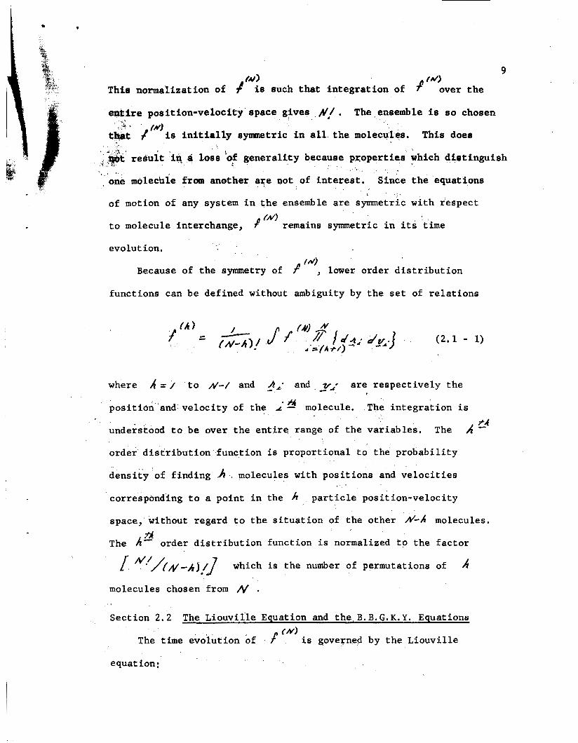
Thie normalization of 1 is such that integration of

en$ire position-velocity space gives N / . The,ensemble is so chosen

'?mer the

/NJ is initially synrmetric in all the molecules. This does

result in ai loss 'af generality because pqoperties which distinguish . 1 . , one molecble from another are not of interest. Since the equations

I ,

of motion of any system in the ensemble are symmetric with respect

to molecule interchange, +''' remains symmetric in its 'time evolu t ion.

f 4 Because of the symmetry of f , lower order distribution

functions can be defined without ambiguity by the set of relations

where A = / to A/-/ and 4,. and zA- are respectively the position and velocity of the A'* molecule. The integration is

understood to be over the entire range of the variables. The 254

order distribution function is proportional to the probability

density of finding .h . molecules with positions and velocities

corresponding to a point in the k particle position-velocity

space, without regard to the situation of the other &A molecules.

The A - order distribution function is normalized to the factor tA

1 N.' / ( M - ~ ) / J which is the number of permutations of 4

molecules chosen from N . Section 2.2 The Liouville Equation and the, E. B. G. K. Y. Equations

The time evolution of f is governed by the Liouville f 4

equat ion:

I

1

1 1

- - /4 -

P T

i - - d P)+ if; = (2 .2 - 1) )r

d t

tu) (4 *

10

are def ined by t he r e l a t i o n s ' 9 4 1

(2 .2 - 2)

and

where nt is the p a r t i c l e mass, M* is t h e momentum of t h e &'a par t icle, is the p o t e n t i a l of i n t e r a c t i o n between molecules

4' and 3' , and Q and 5 are a r b i t r a r y funct ions of t h e

pos i t i on and momentum of the p a r t i c l e s .

t he cont inui ty equat ion f o r po in ts i n pos i t ion-ve loc i ty space.

The L iouv i l l e equation i s

Equations f o r t he t i m e evolut ion of t h e lower order d i s t r i b u t i o n

funct ions are obtained by in t eg ra t ion of t he L iouv i l l e equation:

In theder iva t ion of t hese equations, # (#) i s assumed t o approach

zero r ap id ly as e i t h e r &' o r V i approaches i n f i n i t y . This

set of equations form an i n t e r r e l a t e d h ie rarchy known as t h e

-

t

.R.Y. e q u a t i p e . . To rolve euy one eqy8t+on exac t ly wmld ,

re’a ao lu t ion t+ the o r i g i n a l Liauville equation.

< W e wiah t o d e r e n d n e t h e lower ordgr d i s t r i b r t t ~ o n , f u n c t i o n s of

eystem uniquely 1 . .fa Qenpe of the mecmscopic stat+y fn k i n e t i c

theory t h e number deneaty, stream v e l o c i t y aqd .temperature, which,

when spec i f ied throughout space determine t h e macroscopic s t a t e ,

are s t a t i s t i c a l averages over . However, as. w e have seen,

t h e reduced d i s t r i b u t i o n functions which a r e so lu t ions t o the

B.B.G.K.Y. equations depend u l t imate ly on # .. There are many

choices of the ensemble which give rise t o the same macroscopic

# (4 I

I

s t a t e . Hence the so lu t ion w e wish seems t o be underdetermined.

This is a paradox which u l t imate ly must be resolved i n t h e s t a t i s t i c s

of systems which a r e composed of extremely la rge numbers of molecules,

The reso lu t ion of t h i s paradox has not been carried out completely

s a t i s f a c t o r i l y on a theo re t i ca l basis. Operat ional ly the problem

can be solved by terminat ing the B.B.G.K.Y. h ierarchy and solving

t h e r e s u l t i n g equat:ions on the basis of physical ly re i sonable

assumptions about t h e nature of t h e lower order d i s t r i b u t i o n

funct ions, The e f f e c t of t h i s procedure is t o l i m i t so lu t ions f o r

t he lower order d i s t r i b u t i o n funct ions t o a set of funct ions

determined by t h e macroscopic state.

Sect ion 2.3 Molecular Chaos and t h e Boltrmann Equation \

We now d i scuss a der iva t ion of t he Boltrnunn equation from t h e

/ ‘‘I B. B. G. K. Y. equat iQn. The de r iva t ion involves terminating

t h e B.B.G.K.Y. h ierarchy by t h e so-cal led molecular chaos assumption.

This assumptian is t h a t # ( 2 ) f ac to r s i n t o a product of p t’?

11

12

in those regions of the two particle position-velocity space which

correspond to pre-collision positions and velocities of two particles.

The ratiopale for this assumption is that in a realistic gas there

can be little correlation between t w o molecules prior to their

collieion,

history prior to collisions.

on each other's history after collision.

differentiation between pre-collision and post-collision portions of

the position-velocity space is to introduce irreversibility into

the equations.

That is, they have very little influence on each other's

They, of course, have great inflvence

The effect of this

12 1 It remains to express f everywhere in the two particle

position-velocity space in terms of f") in pre-collision portions of

the position-velocity apace. This can be done by a method used by

Hollinger and Curtire*' based on formal solutions of the

equatione. The A - order B . B . G . K . Y . equation is A4

which can be written

B. B, G. K. Y.

(2.3 - 1)

(2.3 - 2)

14) is the total time derivative considering position and

trl A - Here

velocity coordinates to be implicit functions of time along an 0) ( A 4

order collision trajectory. The quantity J /f ) is a

notation for the rinht side of eauation (2.3 - 1) and 6 is an I- -

13

ordering parameter which w i l l u l t imate ly be ret equal t o one. (4)

We def ine an operator 7 tr ) by t h e relationr

and

(2.3 - I 4)

I A ) The e f f e c t of 7 f r ) on a funct ion is t o transform the

pos i t i on and ve loc i ty var iab les of t he funct ion t o t h e i r value a

t i m e T l a t e r on the A p a r t i c l e t r a j ec to ry . We can then

in t eg ra t e equation (2.3 - 2) and write t h e r e s u l t i n terms of ( A )

T ( r ) ,

For c l a r i t y , we have indicated t h e e x p l i c i t time dependence of t he

operators and d i s t r i b u t i o n functions in equation (2.3 - 5). We now make use of t h e fac t t h a t t h e force between any two

molecules i s purely repuls ive and hence the re are no bound

molecular pa i r s . Then i f 8 - r. is pos i t i ve and s u f f i c i e n t l y

la rge w e can use the molecular chaos assumption t o write

(2.3 - 6)

where the subsc r ip t s on the ~ " ~ s denote the p a r t i c l e t o which

the func t iona l var iab le8 re fer , From equations (2.3 - 5) and

.

14

(2.3 - 6 ) w e have

+ Q

(2.3 - 7) . .. ,,

/4>

Equation (2.3 - 5.) can s i m i l a r l y be used t o express f f f e ) in terms

From equations (2.3 - 7) and (2.3 - 8) we have

I

Equation (2.3 - 9) can be expanded i n an i n f i n i t e power series i n

i f w e assume t h a t a l l d i s t r i b u t i o n funct ions f a c t o r i n t o a product

of

ve loc i ty spaces,

6

!‘‘; B in p r e - c o l l i s i o n regions of t h e i r r e spec t ive pos i t ion-

We can use equation ( 2 . 3 - 5) t o c a r r y out t h e

15 14

f a c t o t i z a t i o n s and transform the t i m e dependence of t h e

manner similar t o what we have done above.

J i n a

We will be concerned with only the f @ term of t h e expansion , '

of f;:;. A l l other terms contai l& t i m e integrations which

are extremely ' d i f f i c u l t t o deal with. I f t h e intermolecular fo rces . L

has a l i m i t as $a+'- which w i l l be denoted by J'". We can

m 0 rep lace f)/t) i n t h e {") B.B.G.K.Y. equat ion by t h e 8 term

' o f equat ion (2.3 - 9). Then i n terms of Sir' we. have

By s t ra ightforward manipulation equation (2.3 - 10) can be transformed

i n t o the ordinary Boltzmann equation plus t h e c o l l i s i o n a l t r a n s f e r

cor rec t ions due t o Green . 7

Equation (2.3 - 10) s u f f e r s from two disadvantages as a

t h e o r e t i c a l d e s c r i p t i o n of gases. F i r s t it takes i n t o account only

b inary c o l l i s i o n s i n t h e sense t h a t i t considers only the t e r m

of t h e series expansion f o r f " ' . Higher terms i n t h e expansion

0

8

r equ i r e e x p l i c i t l y taking in to account t h e dynamics of higher order

co l l i s ions . Second, s ince equation (2.3 - 10) is based on the

molecular chaos assumption, it t a c i t l y ignores bound molecular pairs.

Theore t i ca l ly t h i s d i f f i c u l t y i s overcome by consider ing purely

repuls ive molecular forces . This, however, is not r e a l i s t i c . We

w i l l now develop a formalism which overcomes the f irst disadvantage

of equation (2.3 - 10). The general formalism may a l s o be adequate

16

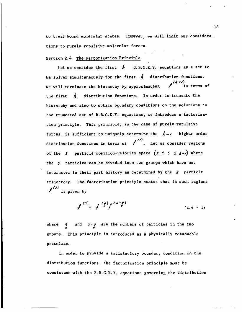
t o treat bound molecular states.

t i o n s t o purely r epu l s ive molecular forces .

€@wever, w e w i l l lkmit our considera-

Sec t ion 2.4 The Fac to r i za t ion P r i n c i p l e

Let us consider t he f i r s t A B.B.G.K.Y. equat ions as a set t o

be solved simultaneously f o r t h e f i r s t 4 d i s t r i b u t i o n funct ions.

We w i l l terminate the hierarchy by approximatsag

t h e f i r s t A d i s t r i b u t i o n func t ions , I n order t o t runca te t h e

/ I A +'in terms of

hierarchy and a l s o t o ob ta in boundary - condi t ions on the so lu t ions t o

t h e truncated set of B.B.G.K.Y. equations, w e introduce a f a c t o r i z a -

t i o n pr inc ip le . This p r inc ip l e , i n t he case of purely r epu l s ive

forces , i s s u f f i c i e n t t o uniquely determine t h e 1-1 higher order

d i s t r i b u t i o n func t ions i n terms of 4 I" . L e t us consider regions

of t he s particle pos i t ion-ve loc i ty space (2 f 5 f A+/> where

the $ particles can be divided i n t o two groups which have not

in te rac ted i n t h e i r past h i s t o r y as determined by the S p a r t i c l e

t r a j e c t o r y , The f a c t o r i z a t i o n p r i n c i p l e states t h a t i n such regions

#"' i s given by

(2.4 - 1)

where f and 3--% a r e the numbers of p a r t i c l e s i n t h e two

groups. This p r i n c i p l e i s introduced as a phys ica l ly reasonable

postulate .

I n order t o provide a s a t i s f a c t o r y boundary condi t ion on t h e

d i s t r i b u t i o n func t ions , t h e f a c t o r i z a t i o n p r i n c i p l e must be

cons is ten t wi th t h e B. B.G.K.Y. equations governing t h e d i s t r i b u t i o n

I

17

funct ions. This consis tency can be shown by consider ing the equat ion

p’ . ,. f o r

From equations (2.2 - 2) and (2.2

and S-g molecules groups of z - 3) it follows tha t , when t h e

are f a r enough separated so t h a t

the p o t e n t i a l of i n t e r a c t i o n between any molecule of one group with

any molecule of t h e o ther is zero, then

I f equat ion (2.4 - 3) is subs t i t u t ed i n t o equation (2.4 - 2) and t h e

fac tored expressions f o r /)(+)and # are a l s o introduced, then,

equat ion (2.4 - 2) is

&+/)

(2.4 - 4)

/z’ Equation (2.4 - 4) is the sum of t h e equations governing / and

p “‘f’. Hence t h e f a c t o r i z a t i o n p r i n c i p l e i s cons is ten t with

the 3.8. Z.K. P. eqiiatlons.

I n order t o use t h e f a c t o r i z a t i o n p r i n c i p l e t o terminate t h e

B.B.G.K.Y. hierarchy, it is necessary t o obta in a form f o r / ‘s)

18

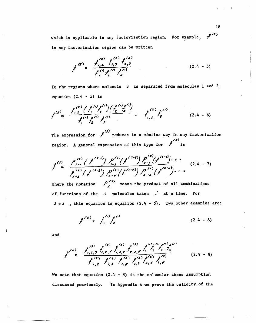
which is appl icable i n any f a c t o r i z a t i o n region. For example, j 3 (3)

i n any f a c t o r i z a t i o n region can be w r i t t e n

(2 .4 - 5 )

I n t h e regions where molecule

equation (2.4 - 5) is 3 is separated from molecules 1 and 2,

The expression f o r +f3’ reduces i n a s i m i l a r way in any f a c t o r i z a t i o n

region. A general expression of t h i s type f o r

where the no ta t ion

of funct ions of t he J molecules taken a t a t i m e . For

S =3

pts’ means t h e product of a l l combinations 4

, t h i s equat ion is equat ion (2.4 - 5 ) . Two o the r examples are:

and

( 2 . 4 - 9 )

We note t h a t equation (2.4 - 8) is t he molecular chaos assumption

discussed previously. I n Appendix A w e prove t h e v a l i d i t y of t he

Equation (2.4 - 7) provides us with a general expression for I A e 4

in all factorization regions. We can.relate 8' in the /&*/I ,

f N+') entire A 91 position-velocity space to f in factorization

regions by a series expansion similar to that developed in

Section 2.3. If we restrict ourselves to the lowkst order term in

19

general equation (2.4 - 7) .

this expansion, we find

This expression for f "+/)in terms of the 4 lower order distribution

function terminates the B. B . G . K . Y . hierarchy. The resulting closed

set of coupled equations are to be solved simultaneously for the

h distribution functions. The factorization principle provides

boundary conditions on these solutions. In the next section we

compare the factorization principle with other methods 06

terminating the B . B . G . K . Y . hierarchy; and we also show that, for

purely repulsive forces, /(*> , fN) ,etc. are uniquely determined in terms of /'')by the factorization boundary conditions.

Section 2 . 5 The Factorization Principle and other Termination

Procedures of the B . B. G . K . Y . Hierarchy

Let us consider the set of equations obtained by terminating

the B . B . G . K . Y . hierarchy with the factorization approximation for

f '33. These equations are:

20

and

(2.5 - 2)

J \ -

If w e consider purely repuls ive forces , t h e r e are no bound molecular

s t a t e e , and hence every t r a j e c t o r y has a p re -co l l i s ion port ion. The

f a c t o r i z a t i o n p r i n c i p l e can thus be appl ied on a po r t ion of every

t r a j ec to ry ,

i n a manner analqgous t o the procedure i n Sec. 2.3,

order ing parameter e i n t eg ra t ion is

This allows us t o formally i n t e g r a t e equat ion (2 .5 - 2)

I n terms of t h e

, introduced i n Sec. 2.3, t h e r e s u l t of t he

21

J

By substituting equation (2.5 - 3) back on itself, we obtain /")as an expansion in terms of /"' and powers of (j . The

time dependences of the singlet distribution functions can be

transformed to time t by the integrated / ":quat ion. This

equation has the form of equation (2.3 - 8). uniquely given in terms of

In this way, /")is

!'.'. This procedure can easily be

generalieed to a set of B.B.G.K.Y. equations truncated at any order.

The Hollinger and Curtiss series expansion for P '* 'was

discussed in Sec. 2.3. The lowest order term in this expansion,

22

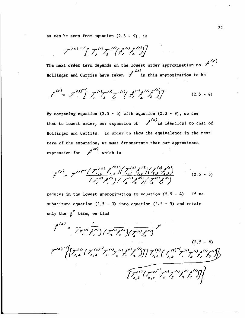
a s can be seen from equation (2.3 - 9), i s

+l /a The next order term depends on t h e lowest order approximation t o . Hollinger and Cur t i s8 have taken / ‘”.’in t h i s approximation t o be

(2.5 - 4 )

By comparing equation (2.5 - 3) with equation (2.3 - 9), w e see / C r )

t h a t t o lowest order , our expansion of is i d e n t i c a l t o t h a t of

Hollinger and Cur t i ss . I n order t o show t h e equivalence i n the next

term of the expansion, we must demonstrate t h a t our approximate

expression for which is

reduces i n t h e lowest approximation t o equat ion (2.5 - 4).

s u b s t i t u t e equation (2.5 - 3) i n t o equat ion (2.5 - 5) and r e t a i n

only t h e p

I f we

0 term, we f ind

(2.5 - 6 )

That is,

(2.5 - 7)

Thus, i f w e terminate t h e B.B.G.R.Y. hierarchy by an approximation

f o r f re-fbtrmally have t h e same expansion as obtained by el

Hollinger and Cur t i ss , through t h e secord term i n t h e i r expansion.

Hollinger and Cur t i s s have shown t h a t t h e Boltzmann equation obtained

by

equation they der ive from t h e

B o g o l u b ~ v ~ ' ~ is i d e n t i c a l t o second order t o t h e Boltzmann f d )

f equation and t h e i r expansion of

f"' . The second order term i n t h e Boltzmann equation derived by

Hollinger and Cur t i s s contains very complex time in t eg ra t ions

involving the dynamics of binary c o l l i s i o n s . To da te , no p r a c t i c a l

ca l cu la t ions have been made on t h e bas i s of t h i s t e r m . Our approach,

however, is somewhat d i f f e r e n t i n t h a t w e do not formally so lve the

/)") equation i n terms of ff". Instead,we so lve the / "' and p /L)

eqbations simultaneously. This can be done approximately and

gives rise t o a s o f t po ten t i a l genera l iza t ion of t he Enskog dense gas

treatment f o r r i g i d spheres . That is, i n t h e l i m i t of r i g i d spheres, 6

t h e Enskog treatment and t h e approximate simultaneous so lu t ion of

t he /''I and / ") equations are iden t i ca l . Thus, our treatment

provides a t i e - i n between two q u i t e d i f f e r e n t approaches t o t h e

problem of th ree body c o l l i s i o n modifications of t h e Boltzmann

equation.

24 Section 2.6 The Dynamics of Binary Collisions

In the present discussion we consider some general properties

of the dynamics of bi,nary collisions between elastic, spherically

symmetric molecules, Again, we restrict our attention to molecules

which interact through purely repulsive forces. The detailed

dynamics of such collisions depend on an intermolecular potential

which is a function of the magnitude of - 4 . The quantity 4

is the radial separation vector. By formulating the problem in the

center of mass coordinates, the interaction can be viewed as that

of a particle with mass “/2 being scattered by a symmetric force center. The non-trivial part of the dynamics is the description

and d of the time evolution of the three scalar quantities 4 ,

“‘f . Here

the scatterer. The dependence on

occurs only in the rotational kinetic energy.

is the velocity of the particle relative to

3 ‘9 in the Hamiltonian f

By making use of the

conservation of angular momentum, we can express the rotational

kinetic energy as a function of only. Thus, for a given

angular momentum, we can conveniently reformulate the problem as a

one dimensional problem. In the reformulation, a particle moves in

one dimension under the influence of a pseudo-potential which ’is the

sum of the true potential and the rotational kinetic energy written

as a function of h . Since the rotational kinetic energy and the

intermolecular potential are both monotonically decreasing functions

of /L , the pseudo-potential decreases monotonically. This

precludes the possibility of bound states.

A typical collision is illustrated in Fig. 1.

E -I

Fig . 1 Dynamics of a Molecular Collision

,

2 6

' approaches the scatterer wi th an d A p a r t i c l e wi th i n i t i a l ve loc i ty

impact parameter ( O r miss distance) 6 . It evetltually passes

through a r a d i a l s epa ra t ton d i e t a w e , J' , which is t h e d i s t ance

of c l o s e s t approach or turning point. F t n a l l y it leaves t h e f i e l d

of fo rce having been scattered through an angle . We note t h a t

t h e c o l l i s i o n t r a j e c t o r y is symmetric about t h e apse l i n e which is a

l i n e through the fo rce cen te r and t h e poin t of c l o s e s t approach.

This symmetry makes i t necessary t o examine only t h e incoming por t ion

-3' of t h e c o l l i s i o n t r a j e c t o r y i n d e t a i l . The angle d between

and 4 on t h e incoming port ion of t he c o l l i s i o n t r a j e c t o r y

conveniently descr ibes the t r a j ec to ry . It follows from t h e d i f f e r e n t t a l

equations which govern the c o l l i s i o n t h a t 25

(2 .6 - 1)

. The quant i ty dm is t h e largest value of OC and occurs when

a= 5 . I n order t o perform c e r t a i n numerical computations discussed i n

and 4 Chapter V, w e need expressions f o r t he s c a l a r products j? R 9*1 .i where t h e symbol A i nd ica t e s a u n i t vector . These

s c a l a r products are conveniently determined i n terms of t he q u a n t i t i e s

/ > b ' X ' 1 9 1 and tp which i s t h e angle

between 4 and -# , These q u a n t i t i e s can be w r i t t e n i n terms

of t h e independent va r i ab le s f ' LF d

and 4 . The va r i ab le s / 3 and J' determine a t r a j e c t o r y and R determines a point on

e i t h e r t h e incoming o r outgoing por t ion of t h i s t r a j e c t o r y , From the

27

is given by d conservation of energy we find that

and from the conservation of angular momentum that

d

and (for U on the incoming portion of the trajectory)

The angle of deflection, 2 , is given by

;2’ = 8 - - z M ,

(2.6 - 2)

(2.6 - 3)

(2.6 - 4)

(2.6 - 5)

(2.6 - 6)

where

integration limit A by f . O ~ H is obtained from equation (2.6 - 1) by replacing the

On the incoming portion of the trajectory it follows from the

definition of ac that

(2.6 - 7) 4

The quantity 7 87 of d and tp by summing the appropriate angles. The fixed

can be determined from geometry and a knowledge

28

s ign of t h e angular momenttin makes t h i s sunmlng uniqqe. We find

(2.6 - 8)

$

The two scalar products on t h e outgoing poytion of t h e t r a j e c t o r y

can be w r i t t e n i n terms of d f o r t he corresponding point on t h e

incoming por t ion of the t r a j e c t o r y and n' . This can be done

because of t h e symmetry of the t r a j e c t o r y about t h e apse l i ne .

We f ind

( 2 . 6 - 9 )

and

z &9s(# ++ostp .+ 3; fiffx)sL4 (2* - 10)

1 It is convenient t o def ine a variabde 9 by the r e l a t i o n

( 2 . 6 - 11)

1 I n words, 3 , i s obtained from R and 3 by f i r s t transforming

n

a r e not i n t e r a c t i n g and then transforming an equal length of time

forward along s i n g l e p a r t i c l e t r a j e c t o r i e s .

- back along t h e two p a r t i c l e t r a j e c t o r y u n t i l t h e two p a r t i c l e s -

We a l s o note t h a t

(2 .6 - 12)

29 m

The coordinate and momentum transformation

is canonixa126 s ince 9 and obey Hamilton’s equat ions f o r

($ , Q> +7 (e/, 5 pl) /

t h e Hamiltonian

That is,

and

(2 .6 - 13)

(2.6 - 14)

(2 .6 - 15)

Physical ly , t h e t ransformation can be seen t o be canonical s ince it

is t h e r e s u l t of two successive canonical transformations.

These a re t h e backward and forward t ransformations along the

t r a j e c t o r i e s mentioned above.

An important property of a canonical t ransformation is t h a t i t s

Jacobian is unity.

space can the re fo re be c a r r i e d out equal ly w e l l by i n t e g r a t i n g

In t eg ra t ions over t h e e n t i r e pos i t i on -ve loc i ty

o r t h e e n t i r e ’ domain of f over the e n t i r e domain of 9 and

A’ # and j ’ . The coordinates 2 ‘ and $’ form a p a r t i c u l a r l y

convenient s e t of i n t e g r a t i o n v a r i a b l e s because they allow us t o

i n t eg ra t e over t r a j e c t o r i e s . The v e l o c i t y ‘(as diecussed above) 9 is t h e i n i t i a l v e l o c i t y and is a constant of the motion. The

1 angles of f i x t h e plane of c o l l i s i o n . I f w e write & i n

30

c y l i n d r i c a l q o o r d i w t e r wi th the h -ax is i n t h e d i r e c t i o n of

then

The apgle 6 determines the o r i e n t a t i o n of t he p o l l i s i o n plane.

The impact parameter, b, which i s a constant of the motion along

' , detgrmines a t r a j e c t o r y i n the c o l l i s i o n plane. The with 9 var i ab le s p e c i f i e s the pos i t ion on the t r a j e c t o r y and is simply

r e l a t e d t o the time by

(2 .6 - 17)

The Poisson bracket is invar ian t i n form under a canonical

transformation. If w e consider i n p a r t i c u l a r the Poisson bracket

1 ~ Iv/ expressed i n the systems ( A C!

we obta in the d i f f e r e n t i a l r e l a t i o n

I f A c

above, and i f

is expressed i n t h e c y l i n d r i c a l coordinate system mentioned

' is expressed i n polar coordinates, then t?

Equations (2 .6 - 18) and (2.6 - 19) show t h i s well-known r e l a t i o n ;

t h a t t he operator

a funct ion of 2 and

[ , f l y gives t h e imp l i c i t time d e r i v a t i v e of

f .

31

For t h e computations discussed i n Chapter V, w e need expressions / A

f o r the scalar products A . A and 3 . d . L e t us de f ine a

quant i ty &%/ as t h e absolute value of t h e t i m e required f o r a

p a r t i c l e t o t r a v e l from t h e tu rn ing point , f , t o t h e point R

on t h e t r a j e c t o r y . L e t us a l s o de f ine - as t h e d i f f e r e n c e

i n t h e t i m e required f o r a p a r t i c l e t o t r a v e l from some p r e - c o l l i s i o n

-

4 @

I'

point on t h e t r a j e c t o r y t o t h e d i s t ance of c l o s e s t approach, and

, t h e t i m e required t o reach t h e d i s t ance of c l o s e s t approach i f no

c o l l i s i o n occurs. The quan t i ty - i s r e l a t e d t o t h e energy

d e r i v a t i v e of t h e quantum mechanical phase s h i f t . Further , l e t us

A @

c?'

d e f i n e b as t h e vec to r from t h e s c a t t e r e r t o t h e d i s t ance of

c l o s e s t approach on t h e non-col l is ion t r a j e c t o r y . Then, &' on

t h e 'incoming port ion of t he t r a j e c t o r y can be w r i t t e n

-

and thus,

and

On t h e outgoing po r t ion of t he t r a j e c t o r y w e have

(2.6 - 20)

(2 .6 - 21)

(2.6 - 22)

(2 .6 - 23)

and

(2.6 - 24)

(2 .6 - 25)

*/ 4 A / r\ The scalar products j A and 7 are g$ven by equations (2.6 - 7) ,

( 2 . 6 - 8 ) , ( 2 . 6 - 9) and (2.6 - 10). We now give analytic forms for &< , 4 4

A d , ,b *k and 9 * f . The time, tA+z required for a particle to go U 27

from /L to A on the incaning portion of the trajectory is

and

Hence,

( 2 . 6 - 26)

where is a pre-collision separation dirtance. We cbn write

33

On passing t o t h e limlt. R + @ , w e have

A 4 We can f ind t h e s c a l a r p r d u c t s ,6 04 and ,b * J i n a

manner analogous t o t h a t used t o f ind J A

the incoming por t ion of t h e t r a j e c t o r y

A / 4 A and i' 0 % , On

and

(2.6 - 31)

On t h e outgoing po r t ion of t h e t r a j e c t o r y

and

(2.6 - 33)

/ 4 / f l and 4 8 These r e l a t i o n s determine the s c a l a r products 4 . A

on both the incoming and outgoing port ions of t h e t r a j e c t o r y .

-

Sect ion 2.7 The T r u n c a i ~ o n e ~ f t h e B.B.G.K.Y. Equations - The F i r s t

Order Approximation

The development i n See. 2*4 provides a formalism f o r f ind ing t h e

lower order d i s t r i b u t i o n functions by so lv ing a t runcated set of

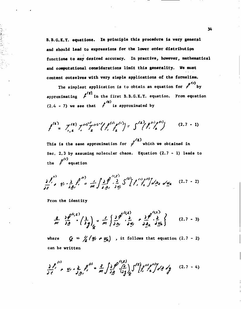
B. B. G. K.Y. equationq. In pr inc ip l e t h i s procedure $8 very genergl

and should lead t o expressions f o r the lower order d i r t r i b u t i p n

funcqioae t o any dealred accuracy.

and ccqmfat4onal conriderat ions l i m i t t h i s genera l i ty .

content ou tse lves wi th very simple appl ica t ions of the formalism.

I n pyactive, however, mgthematical

We murre

The simplest app l i ca t ion is t o ob ta in an equat ion for /"'by p l

approximating i n t h e f i r s t B.B.G.K.Y. equation. From equation

(2.4 - 7) w e 8ee t h a t f '*) i s approximated by

42 1 This is t h e same approximation fo r # which w e obtained i n

Sec. 2.3 by assuming molecular chaos. Equation (2.7 - 1) leads t o

the /I")equat ion

From the i d e n t i t y

where

can be w r i t t e n

@ s & (9 j rs} , it follows t h a t equat ion (2.7 - 2)

It i s convenient t o introduee t h e n o t a t i o n

(2.7 - 5)

where h i s an a r b i t r a r y funct ion of t he va r i ab le s A, , <z , - Zr, and zfz . We note t h a t s p e c i a l cases of t h i s d e f i n i t i o n are - -

(2.7 - 6)

and

(2.7 - 7)

which i s cons i s t en t wi th t h e no ta t ion of Sec. 2.6. Thus equation

(2.7 - 4 ) can be w r i t t e n

We assume t h a t !"Lt any point i n t h e pos i t ion-ve loc i ty space i s

uniquely determined by specifying /L g and 7- everywhere i n

t h e system, That i s /"'is determined by t h e macroscopic state.

It then follows t h a t depends on space and t i m e only through

t h e macroscopic s ta te . I f l 2 , and 7'- are assumed t o be

a n a l y t i c functions of space, then a knowledge of t h e macroscopic

s t a t e i s equivalent t o a knowledge of , g and T and t h e i r

space gradients a t a point. A t equi l ibr ium n , ,u and 7- are

constant throughout space. Thus, from equation (2.7 - 8), t h e

equilibrium equation f o r P ''I is

.

36

The s o l u t i o n t o equation (2.7 - 9) is

(2.7 - 9)

(2.7 - 10)

where r// = ?/ . The quan t i ty i s known as t h e pecu l i a r .-

veloc i ty .

As was discussed i n t h e Introduct ion, t h e t r anspor t c o e f f i c i e n t s

arise from a linear approximation f o r t h e dependences of t h e energy

and momentum f luxes on gradients wi th in the system. The l i n e a r

approximation is va l id only when g rad ien t s i n the system a r e not

t oo large, or, equivalent ly , when t h e system is c lose t o equilibrium.

This suggests t h a t equat ion (2 .7 - 8 ) should be solved i n a

per tu rba t ion expansion of some s o r t about t he equi l ibr ium so lu t ion .

The p a r t i c u l a r method of expansion w e consider is due t o Enskog 5 . On t h e one hand, i t is based on phys ica l i n t u i t i o n ; and on t h e o ther ,

on t h e s a t i s f a c t i o n of c e r t a i n mathematical requirements.

expansion is convenient because i t l i n e a r i z e s equation (2 .7 - 8 )

The

and thus makes it more t r ac t ab le .

L e t us assume t h a t #")is given by the expansion

(2 .7 - 11)

where 6 is an expansion parameter which marks t h e order of

37 1 4 )

perturbat ion. as given by equation

(2.7 - 11) , E w i l l be s e t equal t o one. The equi l ibr ium s ta te i s

I n the f i n a l expression f o r #)

character ized by a lack of s p a t i a l g rad ien ts . Hence, it seems

reasonable t h a t devia t ion from equi l ibr ium should be marked by the

o rde r of s p a t i a l g rad ien ts i n the system,

r i g h t s ide of equation (2.7 - 8) i n a Taylor series about A , c and b

write siiccessive orders i n t h e gradient +

corresponding power of e . This expansion of (2 .7 - 8) y i e l d s

Therefore, w e expand t h e

propor t iona l t o t h e d h f c

(2.7 - 12)

- /.> / The ba r over t h e funct ions <''';nd fi i nd ica t e s t h a t t h e space

v a r i a b l e a t which they are evaluated i s R , . The l e f t s i d e of

equation (2.7 - 12) i s w r i t t e n propor t iona l t o 6' because t h e

operat o r {$-& t f i . 4 3 i s f i r s t order i n t h e grad ien t - J & . That t h i s i s t r u e f o r - 9

f "' depends on time only through

, follows from t h e f a c t t h a t c

2 A/ .- d t

, and 7 and t h e i r

s p a t i a l gradients . From the equations of change, t h e t i m e

de r iva t ive of these q u a n t i t i e s i s propor t iona l t o - b d A , ' c

If equation (2.7 - 11) i s s u b s t i t u t e d i n t o equat ion (2.7 - 12)

38

we can write t h e r e s u l t as a series of i n t e g r a l equat ions which are

t h e c o e f f i c l e n t s of t h e various powers o f € The e equat ion is 0

As is t o be expected ( s ince our method of so lu t ion is a pe r tu rba t ion

expansion about t he equilibrium so lu t ion) equat ion (2.7 - 13) is

i d e n t i c a l t o equat ion (2.7 - 9) and has t h e s o l u t i o n

(2 .7 - 14)

This equat ion states t h a t t o lowest order i n t h e per turba t ion t h e

v e l o c i t y d i s t r i b u t i o n is Maxwellian. The q u a n t i t i e s A , and

7 terms of f

are considered here t o be l o c a l p rope r t i e s and are defined i n f 4

by t h e r e l a t i o n s

and

(2 .7 - 15)

(2.7 - 16)

(2 .7 - 17)

(A Since t h e equi l ibr ium form of 4 must a l s o obey equations

(2 .7 - 15), (2.7 - 16) and (2.7 - 17), these equat ions are s a t i s f i e d /J)

i f w e rep lace /'*'by t L o j . Hence, w e r equ i r e a s add i t iona l

condi t ions on t h e per turba t ion expansion of equat ion (2.7 - 11) t h a t

39

and

a = / (2.7 - 18)

(2.7 - 19)

(2.7 - 20)

It is possible , however, t o r equ i r e t,,e s t ronger condi t ions t h a t

(2.7 - 21)

and

(2.7 - 22)

(2.7 - 23)

These conditions uniquely determine t h e pe r tu rba t ions i n terms of

f i , g and 7 and a l s o insure t h a t equat ions (2.7 - 15), (/ 1

(2.7 - 16) and (2.7 - 17) are s a t i s f i e d by / t o any order of

appr ox imat ion.

The remaining equat ions corresponding t o € / , 6 L , e t c . a r e

/ l i n e a r , inhomogeneous equat ions. The e equat ion is

(2.7 - 24)

It can be shown from the theory o f integral equations 28 that a

necessary and sufficient condition for the solubility of equation

(2.7 - 24) io that the inhomogeneity J , defined by

(2.7 - 25)

'40

be orthpgonal

solutions are

to the solutions of the homogeneous

the summational invariants

equation. These

(2.7 - 26)

p*[" = L v, (2.7 - 27)

41

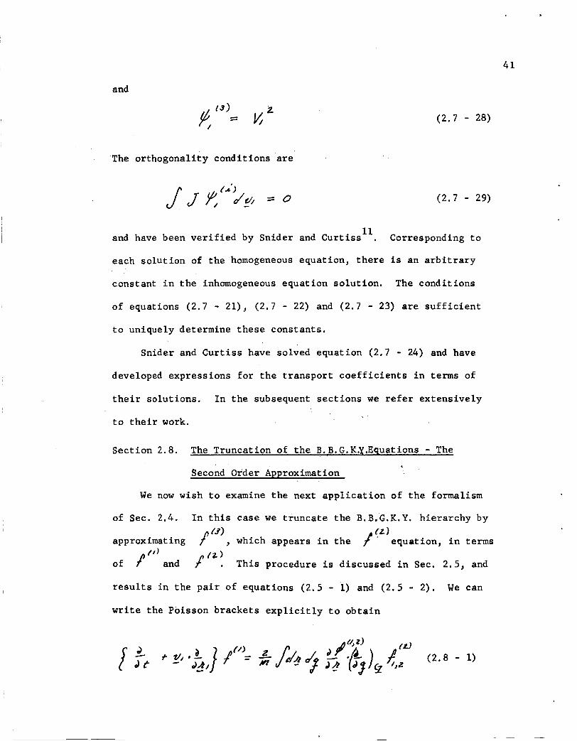
and

(2.7 - 28)

The or thogonal i ty condi t ions are

(2.7 - 29)

11 . and have been v e r i f i e d by Snider and Cur t i s s Corresponding t o

each so lu t ion of the homogeneous equation, t h e r e i s an a r b i t r a r y

constant i n t h e inhomogeneous equat ion so lu t ion . The condi t ions

of equations (2.7 - 21), (2.7 - 22) and (2.7 - 23) a r e s u f f i c i e n t

t o uniquely determine these constants .

Snider and Cur t i s s have solved equation (2.7 - 24) and have

developed expressions f o r t he t ranspor t c o e f f i c i e n t s i n terms of

t h e i r so lu t ions . In the subsequent s ec t ions w e r e f e r ex tens ive ly

t o t h e i r work.

Sect ion 2.8. The Truncation of t he B.B.G.K.y.Equations - The I

Second Order Approximation

W e now wish t o examine the next app l i ca t ion of t h e formalism

of Sec. 2.4. I n t h i s case w e t runca te the B.B.G.K.Y. h ierarchy by

approximating

of !'*' and f '*! This procedure i s discussed i n Sec. 2.5, and

f " I , which appears i n t h e f' fz)equat ion, i n terms

r e s u l t s i n the p a i r of equations (2 .5 - 1) and (2 .5 - 2). We can

w r i t e the Poisson brackets e x p l i c i t l y t o ob ta in

42

and

I n Equations (2.8 - 1) and (2.8 - 2), d, and A, a r e t h e gross

v e l o c i t y and pos i t i on coordinates; whereas

r e l a t i v e t o .u/ and 4) . Since t h e macroscopic s t a t e uniquely

determines I"', it follows t h a t t h e dependence of ! "o>n t h e

- - and R a r e coordinates ae

-

gross pos i t i on and t i m e only can be through the macroscopic s t a t e .

This r e s u l t is more general than is s t a t e d above. It app l i e s

t o a d i s t r i b u t i o n func t ion of any order and i s not dependent on how

t h e gross pos i t i on coordinate i s chosen. To see t h i s , l e t us

consider an 4 p a r t i c l e system and t h e two general

where a' = / fo A . Here and y a r e t h e

coordinates i n the two systems and the sets f_F;'f

s e t s of r e l a t i v e coordinates. The coordinates ,Z, c

t r a n s format ions

(2.8 - 3)

gross pos i t i on

and #&'j? are

and d'/ a r e

taken as the l i n e a r l y dependent p a i r and i t i s assumed t h a t

is no t a func t ion of y -- 4 v , If t he total sys+-eE! llUr $ 1 of '

undergoes a t r a n s l a t i o n , only t h e gross pos i t i on coordinates

and - Y are changed. That is, t he coordinate sets J g f a n d {fif &

4 3

remain unchanged. Thus, i n t h e t ransformation equations any r e l a t i v e

coordinate must be a funct ion s o l e l y of the s e t of r e l a t i v e

coordinates )pel and v i c e versa .

h

- 1 From t h i s i t follows t h a t i f t he

p a r t i c l e d i s t r i b u t i o n func t ion depends on the gross pos i t i on i n

one coordinate system only through t h e macroscopic state, t h i s a l s o

must be t r u e i n the o ther system.

Let us consider t he operator

(2 .8 - 4 )

hi which appears on the l e f t s i d e of t he 4 - order B.B.G.K.Y. equation.

It is s t ra ightforward t o show t h a t t h i s opera tor i s inva r i an t i n

form under any l i n e a r transformation. I n p a r t i c u l a r , i f w e consider

one of the transformations of equation ( 2 . 8 - 3 ) , w e have

where the dot above a pos i t i on vec tor denotes the corresponding

ve loc i ty . Since the p o t e n t i a l of i n t e r a c t i o n i s a func t ion of only

t h e r e l a t i v e coordinates I..;f, i t follows t h a t t h e opera tor

[ , / / ‘yNihich appears on the l e f t s i d e of t h e A B order

B.B.G.K.Y. equation depends on t h e gross pos i t i on and v e l o c i t y only

through the opera tor AI* - * d . A t equi l ibr ium n , - u and 7-

a r e constant throughout space. Thus t h e equi l ibr ium equat ions

f o r t h e d i s t r i b u t i o n func t ions a r e w r i t t e n by omit t ing the opera tor

- d,K

44

from the left Bide of% tP ili ..

r - then are

and

(2 .8 - 6)

(2.8 - 7)

These coupled equations have the solutions

( 2 . 8 - 8)

and

where through first order in the density

y m = e

We note t h a t

form as i n equation ( 2 . 7 - 10). The funct ion

f "'at equilibrium maintains t h e same Maxwellian

CY depends O n l y

45

on

t h e magnitude of t he r a d i a l s epa ra t ion dis tance. As defined i n

is t h e r a d i a l d i s t r i b u t i o n function. 8 equation ( 2 . 8 - 9),

Equation (2.8 - 7 ) , however, i s only an approximate equation f o r

This approximate equation y i e l d s the exact r a d i a l d i s t r i b u t i o n

function t o order t2 i n t he d e n s i t y (as given i n equation (2.8 - l o ) ) .

Livingston and curt is^^^ have examined higher terms i n t h e so lu t ion

. J

of t h e approximate equation f o r r i g i d spheres.

It i s convenient t o wr i te /lL'in terms of a funct ion y defined by

(2.8 - 11)

From equations (2.8 - 8) and ( 2 . 3 - 9) w e f i nd t h a t

equilibrium l i m i t of y , is

yLoj,the

Equations (2.8 - 1) and (2.8 - 2) are d i f f i c u l t t o solve (4

simultaneously, because i n general t h e f a c t o r !f as w e l l as f i n equation (2.8 - 11) is perturbed from i t s equi l ibr ium value

when t h e system i s no t a t equilibrium, However, i t i s poss ib l e t o

so lve equation ( 2 . 8 - 1) approximately f o r /"' by assuming

46

Here t h e coordinate ! is the cenqer of nus@ coordinate and is

def ined by

(2.8 - 13)

I n our equi l ibr ium approximation f o r t h e func t ion y , t h e

q u a n t i t i e s #t and 7 i n equation (2.8 - 12) are funct ions of t h i s

gross pos i t i on coordinate.

way i n order t h a t equat ion (2.8 - 11) r e t a i n i t s symmetry i n

p a r t i c l e s 1 and 2.

is one,

The gross dependence is chosen i n t h i s

We note tha t t h e lead term i n the dens i ty of

This lead term when subs t i t u t ed i n t o equation

(2.8 - 11) gives rise t o t h e molecular chaos expression f o r f'f' S e t t i n g y J y r e J g J 4) can be thought of a8 the f i r s t s t e p

i n an iterative so lu t ion of equations (2.8 - 1) and (2.8 - 2) .

F i r s t under t h i s approximation, equation (2.8 - 1) is solved f o r

p"' . Then, t h i s approximate expression f o r /"' is subs t i t u t ed

i n t o equation (2.8 - 2) which i n tu rn is solved for y . This

so lu t ion is then subs t i t u t ed i n t o equation (2 .8 - 1) and the

i t e r a t i v e procedure i s repeated.

t h a t i t i s d i f f i c u l t t o decide if such a procedure is convergent.

It should be pointed out , however,

Sect ion 2 . 9 The Rigid Sphere L i m i t and the Enskog Dense Gas Equation

( E , & ) fo r t h e

We now show t h a t i n t h i s approxima-

i s given by

Y = %el L e t us consider t he approximation

spec ia l case of r i g i d spheres.

ticn and t o t he order in the dens i ty which

equation (2.8 - 12), equation (2.8 - 1) reduces t o t h e Enskog

6 equation f o r dense gases .

y

Thus our treatment can be thought of as

47

a s o f t p o t e n t i a l gene ra l i za t ion of t h e Enskog treatment.

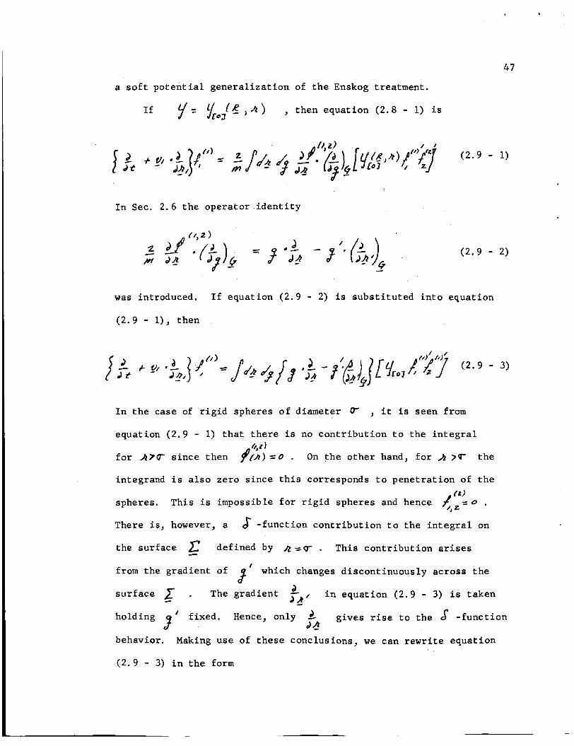
I f y 5 go;R A ) , then equation ( 2 . 8 - 1) i s

I n Sec. 2 . 6 t h e operator i d e n t i t y

( 2 . 9 - 2)

was introduced. I f equation ( 2 . 9 - 2) i s subs t i t u t ed i n t o equation

( 2 . 9 - l), then

I n t h e case of r i g i d spheres of diameter W , it i s seen from

equation ( 2 . 9 - 1) t h a t t h e r e i s no con t r ibu t ion t o t h e i n t e g r a l

f o r s ince then f;!))=O . On t h e o the r hand, f o r A 7 T t h e

integrand i s a l s o zero s ince t h i s corresponds t o pene t ra t ion of t h e ( 2 )

spheres, This i s impossible f o r r i g i d spheres and hence f = o . 'J '

There i s , however, a

the surface defined by &=cr . This con t r ibu t ion arises

' from the gradient of

su r f ace . The gradient -

6 - funct ion con t r ibu t ion t o t h e i n t e g r a l on

-L

which changes discontinuously across t h e

i n equation ( 2 . 9 - 3) i s taken t '

- J &

holding ' f ixed . Hence, only 2 gives r i s e t o t h e $ - funct ion 3 J n behavior. Making use of t hese conclusions, w e can rewrite equation

( 2 . 9 - 3) i n t h e form

. ' I . ,

which by Gauer' theorem is

/ On the surface t h e vector A is equal t o R because the - - c o l l i s i o n is instantaneous. Therefore, w e have on the ourface

4 (2 .9 - 6) 4 3 3 6 -

and

4 where & ia a unit vector i n the direction of & . By restr ic t ing

the c o l l i s i o n integral in equation (2 .9 - 5) to an integral over

the surface

f o m

*3 > 0 , we can write equation ( 2 . 9 - 5) i n the

(2 .9 - 8)

49

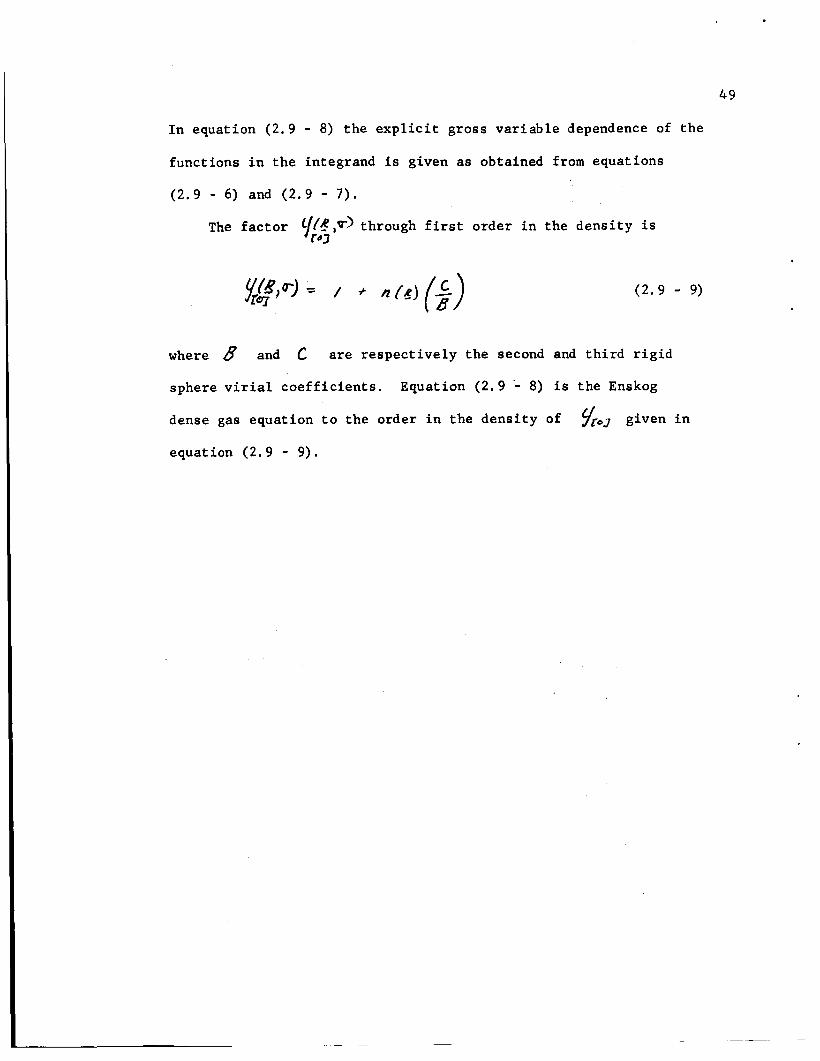
I n equation (2.9 - 8) t h e e x p l i c i t gross v a r i a b l e dependence of t h e

functions i n t h e integrand i s given as obtained from equations

(2.9 - 6) and (2.9 - 7 ) .

The f a c t o r /!f',T> through f i r s t order i n the d e n s i t y i s 403

(2.9 - 9)

where 8 and c are r e spec t ive ly the second and t h i r d r i g i d

sphere v i r i a l c o e f f i c i e n t s . Equation (2.9 -- 8) i s t h e Enskog

dense gas equation t o t h e order i n t h e d e n s i t y of

equation (2.9 - 9).

geJ given i n

CHAPTER TI1

SOLUTION OF THE TRUNCATED B,B.G.K.Y. EQUATIONS

In Sec. 2.8 we discussed an approximate method qf

t he p a i r of equatisas which r e s u l t from t runca t ing t h e

hierarchy at f "? We now solve the 1 equation i n

approximat ion.

Sect ion 3.1 Linear iza t ion of the #'"*quat ion

c*).

(21 I f we approximate f by

s o b t i o n of

t h i s

(3.1 - 1)

then equation (2,8 - 1) becomes

I

In analogy with the procedure i n Sec. 2,8 w e can expand equation

(3.1 - 2) about t h e equilibrium equation. This procedure l i nea r iqe r

equation (3.1 - 2) and thus s impl i f i e s the problem of so lu t ion ,

We again a r r i v e a t a aeries of i n t e g r a l equations.

equation

The lowest order

corresponds, of course, t o the equi l ibr ium equation ( 2 , 8 - 6). The

bar over a funct ion ind ica tes t h a t the gross pos i t ion va r i ab le of

t ha t funct ion is &I . The funct ion has the form

50

- /dJ

51

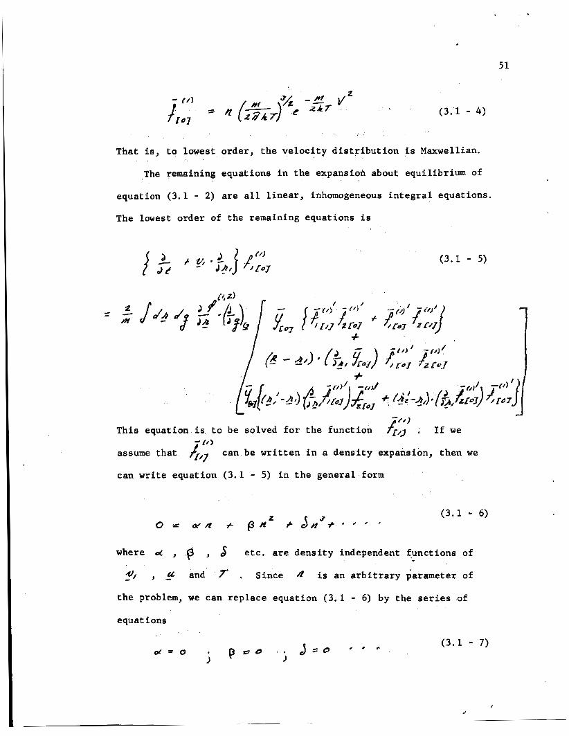
( 3 . 1 - 4 )

That is, to lowest order, the velocity distribution is Maxwellian.

The remaining equations in the expansioh about equilibrium of

equation (3.1 - 2) are all linear, inhomogeneous integral equations. The lowest order ef the remaining equations is

(3.1 - 5)

-//)

This equation is to be solved for the function

assume that j$/7

can write equation (3.1 - 5) in the general form

7$,~ . If we - I t )

can be written in a density expansion, then we

(3.1 - 6)

where d , , $ etc. are density independent functions of

dl > - U. and 7 . Since 4 is an arbitrary parameter of - the problem, we can replace equation (3.1 - 6) by the series of equations

(3.1 - 7)

f

In order t h a t t h e equat ion ot S O be rratisfied, we see from equatdrpn - t#> (3.1 - 5) t h a t t h e leading term i n the expansion of must be

constant in t he densi ty .

%hat SO 'iq an equation for the term o f order /L

depends on the s o l u t i o n of t h e equation d = o ,

Further, w e see from equation (3.1 - 5) - I / )

of $,, and

A similar statement

can be made for each of t h e equations of (3.1 - 7).

our g t t e n t i o n t o the constant and first order terms i n the dens i ty

expansion of t;,~ (and consequently t o the equations tx 3 0 and

Q = u ) equation (3.1 - 5 ) can be simp1tfi .d u

I f w e l i m i t

- ( 4 )

- 8) u l t h equation (2.7 .. 2 4 ) , w e see

eqU8t ioln in t h d - h a a i ty espanr ion

53

(3.1 - 9)

11 Snider and C u r t i s s have shown t h a t pa r t of J can be w r i t t e n

Here 0 is t he second v i r i a l coe f f i c i en t given by

and the tensor 1 is defined by 4 d

(3.1 - 11)

The time de r iva t ives of d , - ci! and 7- whdch appear i n f - //J

can be eliminated by the equations of change, Since /IC~J i s t h e

equilibrium form 4"' , it follows t h a t t h e pressure tensor and

energy f lux vec tor which appear i n the equat ions of change have

t h e i r equilibrium forms. Thus, through terms of order 12 i n the 2

dens it y,

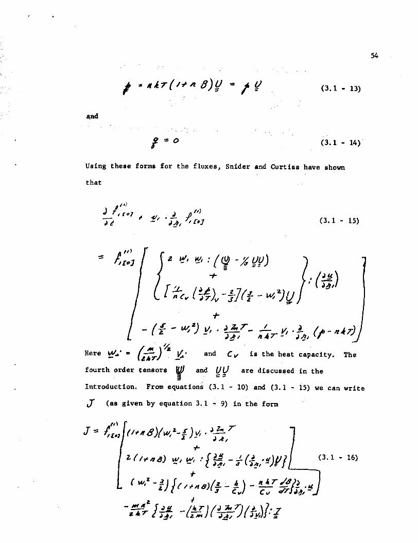
54

and

j 2 = o (3.1 - 14) Using these forms for the fluxes, Snider and Curtiss have shown

that

( 3 . 1 - 15)

Introduction. From equations (3 .1 - 10) and (3 .1 - 15) w e pan write

(as given by equation 3 .1 - 9) i n the form ’ f

55

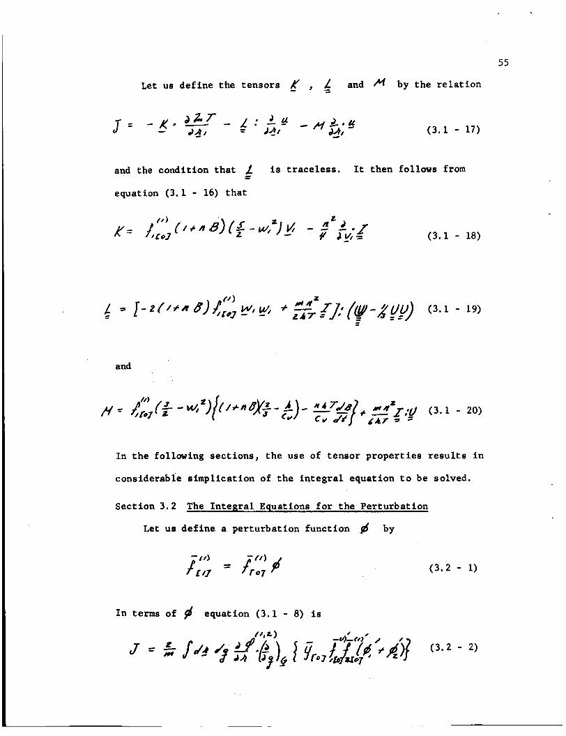
Let us de f ine the t enso r s f - , 4 and A by t h e r e l a t i o n

(3 .1 - 17)

and the condi t ion t h a t - L is t r a c e l e s s . It then follows from

equation (3.1 - 16) t h a t

-

(3 .1 - 18)

and

I n t h e following sec t ions , t h e use of tensor p rope r t i e s r e s u l t s i n

considerable s impl ica t ion of t h e i n t e g r a l equat ion t o be solved.

Sect ion 3.2 The I n t e g r a l Equations f o r t h e Pe r tu rba t ion

Let u s d e f i n e a per turba t ion func t ion pf by

I n terms of equat ion (3 .1 - 8) i s

(3.2 - 1)

56

Let ur ale0 define the linear operator b ' which act# on any

functlon 6 * f/*) by the relation

Equation (3.2 - 2) can then be written

The inhomogeneity, J , given by equation (3.1 - 17) is a linear function of

If followr than that p quantities. Thur we can write

must a180 be c linear function of these

(3.2 - 5 )

where 8 is traceless. Equation (3.2 - 4) io equivalent to the - c set of equation8

(3.2 - 6)

(3.2 - 7)

and

M = A h ) (3.2 - 8 )

57

We now show that the sumnational invariants introduced in equations

(2.7 - 26), (2.7 - 27) and (2.7 - 28) are solutions to the

homogeneous equation

Let us consider the equation

are functionr of only the ecalar A

transformation 3 4 - A . It follow8 from the conrrrvation equations

of a two particle ryrtem that the rumnationrl invariants obey the

relation

and 80 are unchanged by the

, where

ZZ), so (3.2 - 13) and

(3.2 - 14)

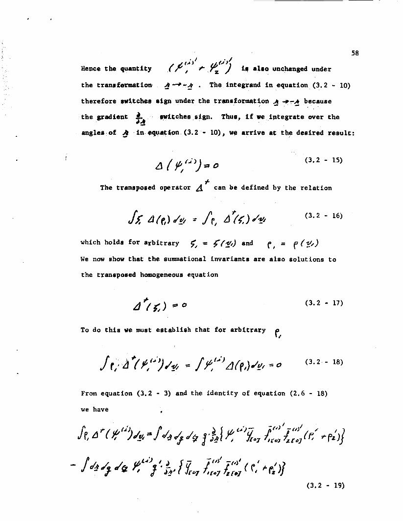
t i / Hence t h e quant i ty (/?''e ) f8 also unchanged under

t h e transfornration * - A . The integrand i n equat ion (3.2 - 10) t he re fo re rwgtches eign under t h e transfortnation 2 +-A because

t h e padicpt & qwffchee sign. Thus, i f w e i p t e g r a t e over t h e

ang1ee.of 3 in ,equaf ton (3.2 - lo), we arrive a t t h e deaired result:

- 4

+?

58

(3.2 - 15)

f The transposed operator can be defined by the r e l a t i o n

(3.2 - 16)

which holds

We now show

for a r b i t r a r y 9, = g(z,) and e , = e (?/)

t h a t t h e summational i nva r i an t s are a l s o so lu t ions t o

the transposed homogeneous equation

e, To do t h i s we must e s t a b l i s h t ha t f o r a r b i t r a r y

(3.2 - 17)

From equat ion (3.2 - 3) and t h e i d e n t i t y of equation (2.6 - 18)

w e have I

59

where 4 = is t h e v e l o c i t y of t he cen te r of m a s s . The

f i r s t integral i n equat ion (3.2 - 19) can be transformed t o a

surface i n t e g r a l on a sphere of s u f f i c i e n t r ad ius such t h a t - %03 / on t h e sur face . This i n t e g r a l is of a type which is

shown t o be zero i n t h e theory of t h e ordinary Boltzmann equation 29 .

Equation (3.2 - 9) can then be w r i t t e n

(3.2 - 20)

We can write equat ion (3.2 - 20) , in t h e symmetric form

(3.2 - 21)

I f w e make the v a r i a b l e t ransformation ( & , f ) -+ (&', 3'J as discussed i n Sec. 2.6, and write 3 coordinate systems given there, then w e have

1 and g' i n t h e p a r t i c u l a r

(3.2 - 22)

The in t eg ra t ion over 3 is an i n t e g r a t i o n over a p a r t i c u l a r

t r a j e c t o r y determined by and d , The q u a n t i t i e s ( efdd> - and

equation (3.2 - l l ) , w e see t h a t t h e integrand is a func t ion of

yIel a r e t h e only func t ions of 3 i n t h e integrand. From

only through t h e dependent v a r i a b l e ~ l t . I f we choose 2 so

60

as t h e cen te r of symmetry of t he t r a j e c t o r y , then

( 3 . 2 - 2 3 )

The integrand of t h e i n t e g r a l i n equat ion (3.3 0 22)

sign under t h e t r a n s f o q t i o n #+ -2

then switches

by v i r t u e of t h e d e r i v a t i v e

. Hence, if w e i n t eg ra t e over 2 we obta in t h e des i red d 32 result:

i s an a r b i t r a r y funct ion, e, or, s ince

( 3 . 2 - 2 4 )

( 3 . 2 - 2 5 )

Since from equat ion ( 3 . 2 - 24) w e have

(3.2 - 26) $U;’’’A($) &, * 0

it follows t h a t if equation (3.2 - 4) is cons i s t en t , then

( 3 . 2 - 2 7 )

From equation (3.1 - 17) we can v r i t e t h e equivalent statements:

( 3 . 2 - 2 8 )

( 3 . 2 - 2 9 )

61

and

(3.2 - 30)

We note from equations (3.1 - 18), (3.1 - 19) and (3.1 - 20) t h a t

t h e tensors x , L I f we then change va r i ab le s from e. t o y, i n equations

(3.2 - 28) , (3.2 - 29) and (3.2 - 30) and i n t e g r a t e over t h e angles

of v, , t he r e s u l t i n g i n t e g r a l s must be i so t rop ic . Since the re

are no i s o t r o p i c odd order tensors and t h e only second order

and hf a r e vec tor funct ions of only f~g . r

I

i so t rop ic tensor c/ ie not traceless, equations (3.2 - 28),

(3.2 - 29) and (3.2 - 30) can be s impl i f ied t o s

0 (3.2 - 31)

(3.2 - 32)

and

f c2/uldg s o (3.2 - 33) - These i n t e g r a l

Equations (3.2 - 31) and (3.2 - 32) r e s u l t from straightforward

in t eg ra t ion ; however, t h e condi t ion i n equat ion (3.2 - 33) is much

condi t ions have been v e r i f i e d by Snider and Cur t i ss .

more d i f f i c u l t t o prove.

t h e i n t e g r a l

J f g : This i n t e g r a l which a l s o

evaluated i n Appendix B,

a r e thus cons is ten t .

The problem involves t h e eva lua t ion of

arises l a t e r on i n t h e treatment is

The i n t e g r a l equations w e wish t o so lve

62

Closely connected with the question of consistency of the

integral equatfons is thit of uniqueness of solution.

a discussion of this important question until the next Qection

We defer

WheFe %t is answered in a natural Qgnrger in the course of the

solution of tho ingegral equations.

The integral equations (3.2 - 6), (3.2 - 7) and (3.2 - 8) can be simplified by considering their teqror properties.

cons$der a second order tensor y

of only the vector W, The tensor must be invariant to a

rotation abouc the axis of d t and hence can depend only on the

isotropic tensor and the dyad If we require in

addition that 5 combination

Let ui \

which io vectorally a function 3

e s

z

be traceless, it must depend on the particular

We can thur write

(3.2 - 35)

where rft,i,j') is a function of the invariant scalar W, . Similar

arguments hold for a tensor of any order.

(3.2 - 6), (3.2 - 7) and (3.2 - 8) depend vectorally on only the vector w, and thus we can deduce their tensor forms. This allows

us to reduce the tensor integral equations to the scalar equations

The tensors in equations

.I)

(3.2 - 36)

63

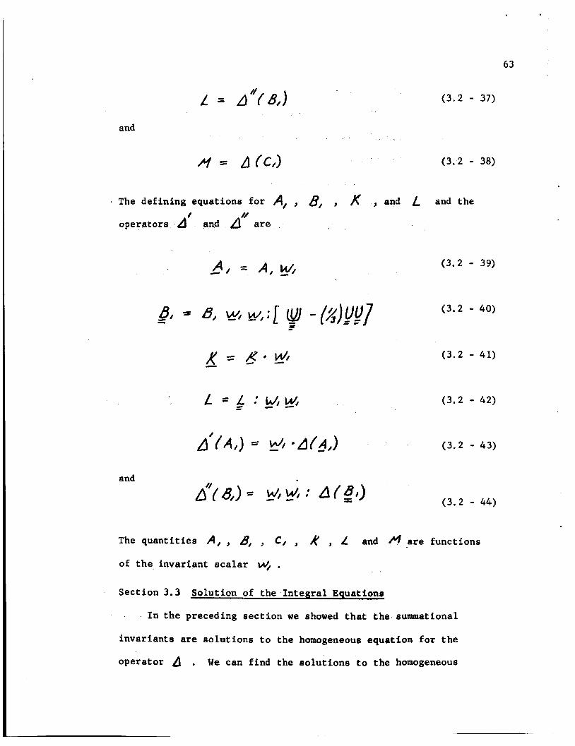
and

(3.2 - 37)

rl 5 (C/> (3.2 - 38)

The defining equations for A, , 8, , , and L and the

operators 4 and are 1 M

and

(3.2 - 39)

(3.2 - 40)

(3.2 - 41)

(3.2 - 42)

(3.2 - 4 3 )

(3.2 - 44)

The quantities A, , 8, , C, , k , L and are functions

of the invariant scalar W, . Section 3.3 Solution of the Integral Equations

I In the preceding section we showed that the summational

invariants are solutions to the homogeneous equation for the

operator . We can find the solutions to the homogeneous

64 f l

equat ions t h a t are func t ions of WI f o r t h e operators , and

// from a knowledge of the general so lu t ions t o t he homogeneous

equat ion f o r t he opera tor d . We f ind t h a t A has t h e homogeneous

so lu t ions 1 and w, , t he opera tor b h a s ' t h e homogeneous

. so lu t ion 1, and t h e opera tor d has no homogeneous so lu t ions .

: { 2. E

/I ..

The transposed opera tors a l s o have these homogeneous so lu t ions .

As w e s h a l l see, t he re i s a one t o one correspon4ence.between t h e

so lu t ions t o t h e homogeneous equations and the a r b i t r a r y constants

i n t h e so lu t ions of t h e i n t e g r a l equations. There are j u s t enougb

a r b i t r a r y parameters i n t h e so lu t ions of t h e i n t e g r a l equations t o

allow us t o impose t h e i n t e g r a l condi t ions of equat ions (2.7 - 21) ,

(2.7 - 22) and (2.7 - 23). L e t us f i r s t consider equation (3.2 - 36). I n order t o so lve

. However, d/ can 1

t h i s equation we must inve r t t h e opera tor

not be inver ted i n a s t ra ightforward manner because i t i s s ingular .

That is, t h e homogeneous equation has a so lu t ion , This problem

can be avoided by wr i t i ng equation (3.2 - 36) i n a matr ix

representa t ion . bet u s expand i n a complete s e t of Sonine

polynomials of order 312. The M A polynomial of t he set of

Sonine polynomials of order d is represented by $, and is

defined by

tk f m )

These polynomials have the or thogonal i ty property

65

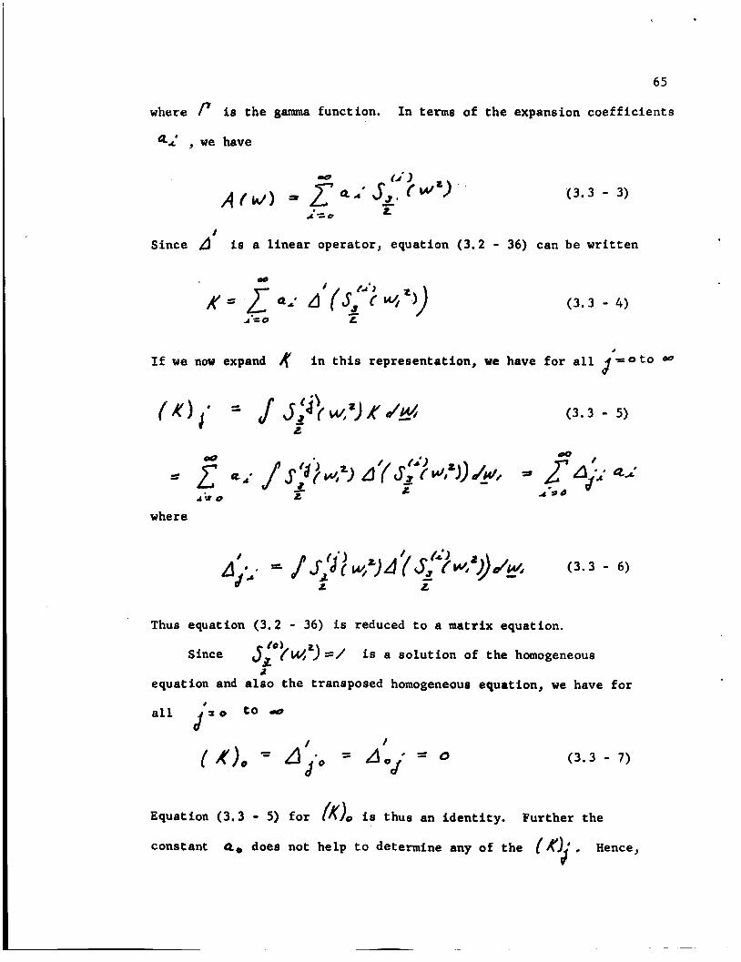
where is the gamma function. In terms of the expansion coefficients

a; , we have

'(3.3 - 3)

/ Since d i s a linear operator, equation (3.2 - 36) can be written

(3.3 - 4)

' If we now expand 4 in this representation, we have for all s o t o O0 a

(3.3 - 5)

where

Thus equation (3.2 - 36) is reduced to a matrix equation. l o )

Since Jz f w z ) = / is a solution of the homogeneous equation and also the transposed homogeneouo equation, we have for

all to d

2

(3.3 - 7 )

Equation (3.3 - 5) for (K)o is thus an identity. constant

Further the

a. does not help to determine any of the ( K ) ' 4 Hence,

we can ignore the farst

The new matrix

66

row and the firet CQL- o f the matrtx

J * l S / to * A'3.H to .o ha8 no

zerO eigenvalues and thus i s non*singuJab and can be invprted.

Equation (3.3 !i)# when inverted, can be written for tq cD ., . - . a ' , I , * ,

r/ # b &

where (d%k' is the A - element of the inverted matrix. Thus A, is given by

a

where (L. is an arbitrary constant. We f ix by the relation

(3.3 - 10)

discussed in Sec. 2.7. Because of the orthogonality condition of

equation ( 3 , 3 - 2) the integral relation of equation (3.3 - 10) requires

' .

a. = o (3.3 - 11)

We can solve equations (3.2 - 37) and (3.2 - 38) by the same technique.

polynomials the Sonine polynomials or order 5/2.

has no solutions to its homogeneous equation,

immediately invert its matrix representation and obtain the

expression for 8, :

To solve equation (3.2 - 37), we use as expansion

The operator

Hence, we can

67

( 3 . 3 - 12)

To solve equation ( 3 . 2 - 38) , we choose as expansion polynomials

the Sonine polynomials of order 1/2. The operator d has two

solutions to it8 homogeneous equation. These two solutions

/ b 4 = can be written as a linear combination of the

first two Sonine polynomials: S:'?M?)=/ and s-!')w,t) A L - = / f - . We obtain a non=singular matrix

by ignoring the first two //

from the matrix representation of d rows and columns of the matrix. We then obtain the expression for C,

where Co and C , are arbitrary constants. These constants are

uniquely determined by the relations

and

(3.3 - 14)

( 3 . 3 - 15)

which were discussed in Sec. 2.7. Because of the orthogonality

condition of equation ( 3 . 2 - 2) we have

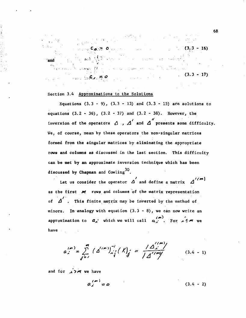
68

( 3 . 3 - 17)

Section 3 . 4 Approximations to the Solutions

Equations ( 3 . 3 - 9 ) , ( 3 . 3 - 13) and ( 3 . 3 - 15) are solutions to equations ( 3 . 2 - 3 6 ) , ( 3 . 2 - 37) and ( 3 . 2 - 3 8 ) . However, the

// inversion of the operators .Ls , A' aild d presents some difficulty.

We, of course, mean by these operators the non-singular matrices

formed from the singular matrices by eliminating the appropriate

rows and columns as discussed in the last section. This difficulty

can be met by gn approximate inversion technique which has been 30 .

Let us consider the operator d and define a matrix d

discussed by Chapman and Cowling /

as the first H

of 0' . minors.

row8 and columns of the matrix representation

This finite matrix may be inverted by the method of

1n.analogy with equation ( 3 . 3 - 8 ) , we can now write an c c o 4

approximation to ab' which we will call a; . For ~ 5 1 1 1 we

have

and for ~ ' 7 4 + l we have

( 3 . 4 - 2 )

69 I /*) 0fm b

In Equation ( 3 . 4 - l), /d / is the determinant of 4 and

/ t N ) ' /d / / i r the determinant of the matrix formed from

by for all s tQ m . a' by replacing the elements

The determipant form in equstion ( 3 . 4 - 1) results fram the inversion of 4 '(4 by minorg and I s a standard form of solution

of a system of linear algebraic equigtions. We aeeume that

In the oimplert approximation, where m r i , we have

and for all A * # /

( 3 . 4 - 3 )

( 3 . 4 - 4 )

In an analogous manner, we find that the firat approximation

to b, (which in accord with the above diocureion we denote

by 6:) i r given by

and for A*#o :

&;I E 0

Similarly, the first approximation to ca is

( 3 . 4 - 7 )

70

(3.4 - 8)

and for ~ ‘ $ 1 : :

(3 .4 - 9 ) f” = 0 = L*

- , , .

Section 3.5 Components of the Non-homggeneous Terms

We now evaluate the integrals ( A ) , and (HA. Let us

consider f A(), , which, according to eqvetionr (3.2 - 41) and

(3.3 - 5), is given by

(3.9 - 1)

From the orthogonality condition given in equation (3.2 - 31) we have

(3.5 - 2)

If we substitute the expression for K given in equation (3.1 - 18) into equation (3.5 - 2), we find

7 1

The f i r s t i n t e g r a l i n t h i s expression can be evaluated immediately

and t h e second can be r ewr i t t en by manipulating t h e divergence i n

the integrand, Thus w e have

(3 .5 - 4)

The i n t e g r a l of t he divergence can be converted t o a vanishing

sur face i n t e g r a l y i e ld ing

(3 .5 - 5 )

We can eva lua te fL), and f N j a i n a similar manner t o ob ta in

(3 .5 - 6)

and

In Appendix 8, t he i n t e g r a l s $(I - I U) W',*d@, and -I

j ( , I : y )wY&i are evaluated i n terms of t h e second

v i r f a l coe f f i c i en t , 8 , and i t s temperature de r iva t ives . Thus,

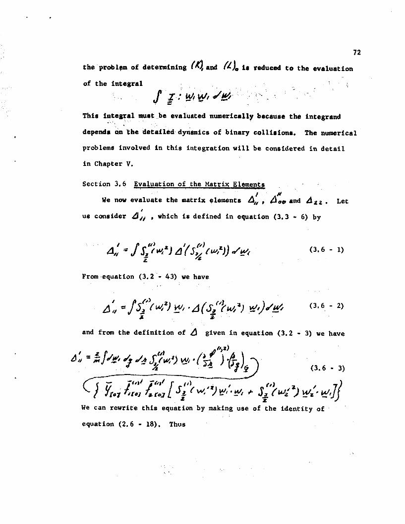
72

t h e p r o b l p of determining (4 and fL), i r veduced t o t h e eva lua t ion

of t h e i n t e g r a l 4 z:%p4&.- a- * - This 4ntegra l must be evaluated numerically because t h e integrand

depends an t h e d e t a i l e d dynamics o f binary co l l l o ions , The numerical

problems involved i n t h i s integrat€on w i l l be considered i n d e t a i l

i n Chapter V,

Sect ion 3.6 Evaluation of the Matrix Elements / El

We now evalua te the matrix elements A,, de, and dzz , L e t /

us consider d,, which is defined i n equation ( 3 , 3 - 6) by

( 3 . 6 - 1)

From equat ion ( 3 . 2 - 4 3 ) we have \ I

and from t h e d e f i n i t i o n of a given in equation ( 3 . 2 - 3 ) we have

(3.6 - 3)

2 z We can r ewr i t e this equation by making use of the i d e n t i t y of

equat ion ( 2 . 6 - 18). Thus

73

(3.6 - 4) +

The f i r s t i n t e g r a l of t h i s equat ion can be converted t o a su r face

i n t e g r a l on a sphere of s u f f i c i e n t rad ius t h a t

surface.

((square braakets" discussed h v Chapman and Cowling3! The square

- 'J,r I on t h e

This su r face i n t e g r a l can be w r i t t e n i n terms of t h e

brackets have been evaluated3* and from these results w e f i nd t h a t

(3.6 - 5)

Here V is an a r b i t r a r y constant wi th t h e dimensions of length.

It i s conveniently chosen as a parameter of t he intermolecular

po ten t i a l and is introduced t o make ~ f r ' Z J * dimensionless. The

reduced omega i n t e g r a l , n"':):s defined by

(3.6 - 6)

L 74

where x P@,& and where b and % are rerpectively the ‘ ,

impact paramet& alba the angle of deflectton.

and X are diecursed in See. 2.6. The integral is a

The quantities b 4 2 P

’ . tabulated function ob the - By the identity of equation (2.6 - 18) we have

(3.6 - 7)

Hence we can write equation (3.6 - 5) in the form:

(3.6 - 8)

Let us make the variable transformation 8 4 L~A . The Jacobian

of this transformation is such that

(3.6 - 9)

If we then write the integral in equation (3.6 - 8) in a form symmetric in part.icles 1 and 2, we have

J, P47- * fZ ,Z)* . 4, 4 - a n 2 2 TT ~ z ~ ~ ) 2 ( ~ ) s R

and

Let us define the vectors / and 3 by the relat ions e

(3.6 - 11)

75

(3 .6 - 12)

Then

( 3 . 6 - 14)

The Jacobian of the transformation (&,) M / L ) 4 / I r) is unity.

Hence, i f we rrubetitute equations (3 .6 - 13) and (3.6 - 14) into

equation (3.6 - 10) we find

- ) - - -

76

(3.6 - IS)

We can integrate over the angles of i? nuking ure of the

fact that

(3.6 - 16)

A

where r ir a unit vector i n the direct ion of - r . Thus w e

have

(3.6 - 17)

(3.6 - 18)

77

and make use of t,he f a c t t h a t .

(3.6 - 19)

. A 0 where 8' i s a un i t vector , then our exp.ression f o r b,, can be

s implif ied t o

The i n t e g r a l over can be ca r r i ed out t o y i e ld

(3.6 - 21)

where

The i n t e g r a l R must be ca lcu la ted numerically. We d i scuss

t h i s ca l cu la t ion i n d e t a i l i n Chapter V,

. I n a manner analogous t o t h e above procedure w e f i nd t h a t

and

(3.6 - 23)

(3.6 - 24)

78

.'. .

4 I The eva lua t ion of t h e matrix elements d r r , 400 and dr.completes

/I> 0) the-deterpptnmtiqn of t h e coe f f i c i en t s a?' , b o and ' q r . .

. .

Sect ion 3.7

I n See,.

l i n e a r terms

equat ion f o r

The Density Expansion of t h e Per turba t ion of the

Dis t r ibu t ion Function

3.1 we r e s t r i c t e d our a t t e n t i o n to t h e constant and

i n t h e dens i ty expansion of 4,~ and s impl i f ied our

I '

r ,

.a .

//>

f / J h , ~ accordingly. Equivalently, w e are j u s t i f ied i n I 4 1 f 4 ) f d )

r e t a in ing only those terms of U , , be and C+ which are of

order or constant i n the densi ty . We note t h a t A (as defined

i n equat ion (3.6 - 22)) is densi ty independent, if only the constant

and l i n e a r terms of

note t h a t 2 and. fl ,(defined respec t ive ly by equations

(3.1 - 12) and (3.6 - 6)) are a l s o dens i ty independent. Then from

our formulae for /#), + (lj0 and [4JZ and the matrix element!

I

$&,J a r e used i n i t s evaluat ion, ,S imi la r ly , w e I ,

tz,zJ* z

1 // d,, , b e e and &a we can c a s t equations ( 3 . 4 - 4 ) , ( 3 . 4 - 6 ) I / ) /A f / l

and ( 3 . 4 - 8 ) which determine 9, , 6, and C, i n t h e general

form:

( 3 . 7 - 1)

f /) 2 (For example w e can write % = Q, , dn f p R (#)( , and / l S R 2 + C d ) ==' A,/ . I f we expand F i n t h e dens i ty ,

we f ind

(3.7 - 2)

through t h e constant term.

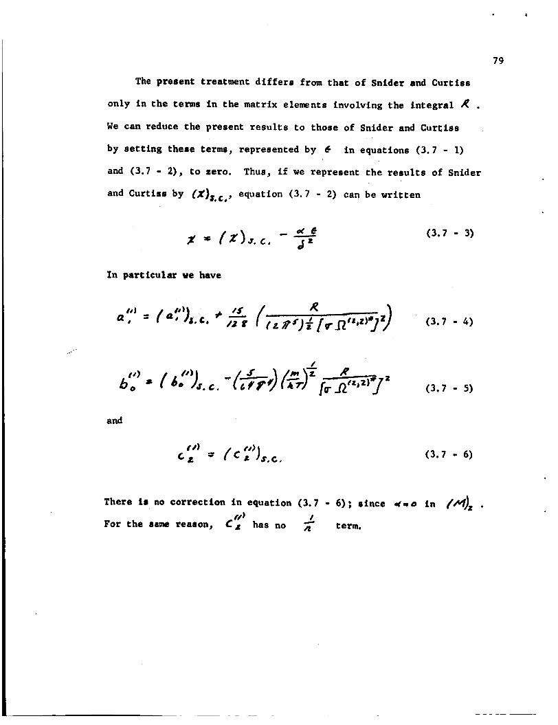
79

The present treatment d i f f e r s from t h a t of Snider and C u r t i s s

only i n t h e terms i n t h e matrix elenrents involving the i n t e g r a l R . We can reduce t h e present r e s u l t s t o those of Snider and Curf ies

L

by s e t t i n g these terms, represented by 8 i n equations (3.7 - 1)

and (3.7 - 2), to zero. Thus, if we represent t h e r e s u l t s of Snider

and Cuttias by (X)s,c, , equation (3 .7 - 2) can be w r i t t e n

I n pa r t i cu la r w e have

and

(3.7 - 3)

(3.7 - 4)

(3.7 - 6)

There is no co r rec t ion i n equat ion (3.7 - 6); s ince 4 9 0 i n {M)z . For t h e same season, C, has no

1 e term.

(0)

CHAPTER IV .- . I

TRANSPORT COEFFICIENTS 1.

In the last chapter we solved an'.approximate + ":quat ion. We ' 2 :

now derive expressions for the transport co&f$ieieatq b&&d on this

solution.

Section 4.1 Flux Vectors

The pressure tensor and energy flux vector represent fluxes of

They arise from the transport of momentum and energy respectively.

these quantities within the fluid in two distinct ways. The kinetic

contribution to the transport ts due to the movement of the individual

molecules and the accompanying transfer of momentum and energy. Since

- .

. the kinetie contributions to the fluxes result. from a uni-molecular . I

process, they can be expressed in terms of the distribution

function f "I. The collisional contributions, on the other hand,

arise from the transfer of momentum and energy from one molecular

center to another by interaction through the intermolecular potential.

Since this is a bi-molecular tranbfer process, the collisional

*

contributions to the fluxes are given in terms of / ".' 33

Irving and Kirkwood have developed general expressions for

the kinetic and collisional contributions t o the fluxes.

expressions, Snider and Curtiss'l have written the fluxes to first

From their

order in a perturbation expansion.

pressure tensor,

The kinetic portion of the

, which we write #& > is

(4.1 - 1) PK - c

80

81

and the coilirtonal portion, #f , is

The total pressure tensor is

Similarly, for the energy flux vector we have -e, (4 .1 - 4)

c -

and

/d J

Through fivrt order i n the perturbation expansion, 4 i s given by

(4 .1 - 8)

and

82

I , 2

where terms of higher order than /E

deleted.

i n t h e dens i ty have been

/,I / / I Since w e have obtained 4,] = through order n i n t h e

densi ty , i t follows from equations (4 .1 - 1) and (4 .1 - 4) t h a t w e

can write t h e k i n e t i c port ion of t h e f luxes t o t h a t .order. Furthermore,

t h e constant t e r m of t he k i n e t i c po r t ion does not involve t h e i n t e g r a l 0) I,)

terms of a, and 60 do not involve R I

/ R because the - n

Similar reasoning shows t h a t we can wri te the c o l l i s i o n a l . port ion of

z t h e f luxes t o order /2. and tha t t o order fl they are independent

of /f .

Sect ion 4,2 The Density Expansiors of t h e Transport Coeff ic ients

The above considerat ions hold a l s o f o r t he t r anspor t c o e f f i c i e n t s

which are simply r e l a t e d t o t h e f luxes as discussed i n Chapter I.

Since t h e t o t a l t r anspor t coe f f i c i en t i s t h e sum of i t s k i n e t i c and

c o l l i s i o n a l p a r t s , i t follows from the remarks of t he las t s e c t i o n

tha t i f t he k i n e t i c p a r t i s non-zero, we can c a l c u l a t e t he t o t a l

t r anspor t c o e f f i c i e n t only through order R . This i s t h e case with

the c o e f f i c i e n t s f and /r . It a l s o follows from t h e last s e c t i o n

t h a t oniy the k i n e t i c portiori ef th2 transport coefficient Lnvolves

t h e i n t e g r a l R t o order n . Since t h e expression f o r t h e

c o l l i s i o n a l po r t ion of t he fluxes t o order fi can be w r i t t e n by

83 - letking , it follows that our treatment to this order gives expressions for the collisional portion of the transport coefficients

identical with those of Snider and Curtiss.

From equations (1 - 11) and (1 - 12) of Chapter 1,we see that is the coefficient of a traceless second order tensor, bi (*&, '3)

is the coefficient o f and A is the coefficient of a first

order tensor. These tensor properties, along with the definitions of

-c

A , # and C given in equation (3.2 - 5), insure that

depends only on the coefficient 6, , 8 depends only on C 2 , c

c 4 f / J

/A and on a, .

c

As w e shall prekently demonstrate, there is no kinetic 2

contribution to H . Thus H can be written to order f i ,

Since , ae given in equation (3.7 - 6), does not depend on

neither doer &t . Also, since C t has no term, we can

set $.~f/ to calculate the collisional contribution to H to

order lt . Thus, our X is identical to that of Snider and

t r ) c a

// 1 /

- a

Curtiss.

Let us examine the kinetic portion of . To do this we

find # A from equation (4.1 - 1).

(4.2 - 1)

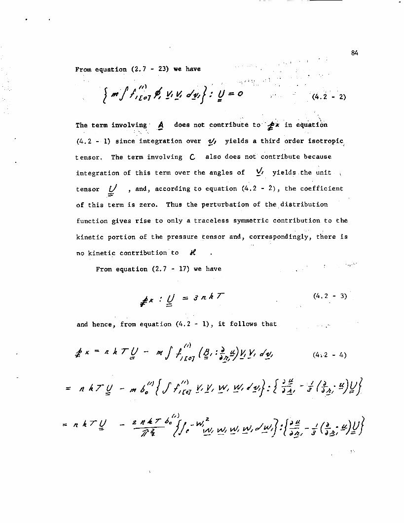
84

From equation (2.7 - 23) we have

The term involving

(4.2 - 1) s ince i n t e g r a t i o n over 2/’

A does not con t r ibu te t o -@ i n equation . e

y i e l d s a t h i r d order i so t rop ic . c

t e n s o r . The t e r m involving C a l s o does not con t r ibu te because

i n t e g r a t i o n of t h i s term over the angles of t/, y i e l d s the u n i t .

tensor I/ , and, according t o equation (4.2 - 2) , t he c o e f f i c i e n t c c

of t h i s term i s zero. Thus the per turba t ion of t h e d i s t r i b u t l o n

funct ion gives r ise t o only a t r a c e l e s s symmetric con t r ibu t ion t o t h e

k i n e t i c po r t ion of t h e pressure tensor and, correspondingly, t h e r e i s

no k i n e t i c con t r ibu t ion t o b4 . . .

-I . From equation (2.7 - 17) w e have

(4 .2 - 3)

and hence, from equation (4.2 - l ) , it follows t h a t . -.

85 A

L e t us consider t he in t eg ra t ion over t he angles of gf . If 4, is

a u n i t vec tor i n the d i r e c t i o n of g~ , then, by symmetry of the

integrand, w e have

where @ is a constant. Further ,

(4.2 - 6 )

Hence, from equations (4.2 - 4), (4.2 - 5) and (4.2 - 6) w e have

where f is t h e rate of shear tensor defined by s

On i n t eg ra t ion over d, , we have

(4.2 - 8)

(4.2 - 9)

From equation (1 - 11) it then follows t h a t t h e k i n e t i c por t ion of

P ’ is given by f , which we write as

(4.2 - LO)

given i n equat ion (4.1 - 4), e. S t a r t i n g w i t h t h e expression fo r

86

I.

? w e f ind i n a similar manner tha t

. 1 .

(4.2 - 11) , .

We then conclude from equation (1 - 12) t h a t

(4.2 - 1 2 )

We can now write t h e t ranspor t c o e f f i c i e n t s i n terms of t he 'i i i

i n t e g r a l 4 *+ I f )

of equations (4.2 - 10) and ( 4 . 2 - 12) and t h e expressions f o r U , , and t h e results of Snider and C u r t i s s by makkng use

> I ; . .

'. I .

(11 I 4 6 0 . and Cz of equations (3.7 - 4 ) , (3.7 - 5 ) and (3.7 - 6) .

We also make use of t he f a c t t ha t our treatment does not a f f e c t t h e

c o l l i s i o n a l por t ions of t he t ranspor t c o e f f i c i e n t s given by Snider

and C u r t i s s . , Thus w e have

? . . .

. . ' r :

. c x I.-

$ , . I

, t

and * ' I

(4.2 - 15)

Here the subscr ip t S.C. denotes the r e s u l t of Snidbr and C u r t i s s .

It i s convenient t o write the d e n s i t y expansion of t h e ' t r a n s p o r t

c o e f f i c i e n t s i n t h e form

87

( 4 . 2 - 17)

and

where arc the cOnstant terms i n the d e n r i t y expanrions 1sL

of A and

e ta , are dimcnrionlers and dens i ty independent and are

f . The q u a n t i t i e s 8: , C E , B;." c;

r e f e r r e d t o as the reduced t r anspor t v i r i a l coe f f i c i en t s . From t h e

d e n r i t y argument8 given previously i n t h i s o p t i o n , we note t h a t

i t i r porrible t o a a l c u l a t e the q u a n t i t i e s lF

A'.', f t0' , &A , f 8; qnd c from our treatment. The q u a n t i t i e s A'Q' and '*)

can be ca lcu la tqd from t h e - ' terms of U, and 6, and equat ions

(4.2 -1'0) a d (4 .2 - 12'3 We f ind t h a t

//I I01 rL

and

(4.2 - 19)

( 4 . 2 - 20)

It then follows from equat ions (4.2 - 13), ( 4 . 2 - 14) and ( 4 . 2 - 151,

t h a t

88

and

(4.2 - 21)

(4.2 - 22)

( 4 . 2 - 23)

In Chapter V we consider the evaluation of these coefficients

for a particular molecular potential and compare the results of a

number of experimental measurements and theoretical calculations.

Section 4 . 3 The Rigid Sphere Limit and the Enskog Dense Gas Transport

Coefficients . We now consider the correction to the results of Snider and

Curtiss for the special case of rigid spheres.

evaluate the integral /p

To do this we

which is defined in equation ( 3 . 6 - 2 2 ) as

From the identity of equation ( 2 . 6 - 18) we have

( 4 . 3 - 2 )

89

We can rewrite R i n the form

From t h e i d e n t i t y of equation ( 2 . 6 - 18) w e have

Thus, the integrand of t h e second i n t e g r a l i n equation (4 .3 - 4 )

Since f o r 4 L g- e -&‘Z)CI , and f o r 70- - b 8‘” = o =)

d A y‘’zh;s a d i s c o n t i n u i t y a t R z u- ; t h i s quan t i ty has a and

3-funct ion behavior a t R = V . We can thus replace yc0;4, 4 1

by

equation (4 .3 - 4 ) .

y r g d i n t h e integrand of t h e second i n t e g r a l i n

We then have

90

Let us now make the variable transformation

From equations (2.6 - 16) and (2.6 - 19) E & , I )+ /e' g/) > -

discussed in Sec. 2.6.

we have

Integration over t. yields

( 4 . 3 - 8 )

which from equation (3.6 - 6) is

For rigid spheres

sc

l2 tzJzj = /

and, from equation (2.9 - 9)

( 4 . 3 - 9)

( 4 . 3 - 10)

( 4 . 3 - 11)

where 8 and C are respectively the second and third rigid sphere

virial coefficients, Thus we have

( 4 . 3 - 12)

and

91

From equations ( 4 - 2 - 2 1 j , 44,2 - 22) a-nb (G.2 2 3 ) , xe kave

( 4 . 3 - 13)

( 4 . 3 - 14)

(4.3 - 15)

The Enskog dense gas equation f o r r i g i d spheres, which i s given

by equation ( 2 . 9 - 8) , d i f f e r s from the ordinary Boltzmann equation

i n two respects. F i r s t , i n t he ordinary BoPtzmann equation, t he

product of one p a r t i c l e d i s t r i b u t i o n funct ions i n t h e c o l l i s i o n i n t e g r a l

are evaluated a t t h e gross pos i t i on - A, . Second, t h e f a c t o r

(JcD7 i n t h e ordinary Bolttmam equation i s uni ty . Snider and

Curt iss34 have shown t h a t t he t r anspor t v i r i a l c o e f f i c i e n t s # (dl)s c, (8;)x,c- and ( C X ) ~ , ~ , i n t he s p e c i a l case of r i g i d

spheres, a r e i d e n t i c a l t o those obtained by d i r e c t s o l u t i o n of t h e

Enskog equation when t h e dev ia t ion of yfp7 from u n i t y i s not

considered. Our treatment i n t h i s l i m i t gives r i s e t c j t h e f u l l

t r anspor t v i r i a l c o e f f i c i e n t s obtained from t h e Enskog treatment

through the inc lus ion of the co r rec t ion - c L i n t h e c o e f f i c i e n t s V-? 49

85 and 8; . This co r rec t ion a r i s e s from the l i n e a r term i n

CHAPTER V

EVALUATION OF THE TRANSPORT COEFFICIENTS

I n t h i s chapter w e consider t h e t r anspor t c o e f f i c i e n t s of a gas

composed of molecules which i n t e r a c t through a real is t ic p o t e n t i a l

which i s repuls ive at shor t separat ions but i s a t t r a c t i v e a t l a rge

separat ions. The t h e o r e t i c a l development i n the preceding chapters

i s appl icable only t o purely repuls ive p o t e n t i a l s , We can, however,

s epa ra t e ly consider contr ibut ions t o t h e t r anspor t c o e f f i c i e n t s which

arise from bound states and non-bound states. The non-bound s ta te c o n t r i -

but ions can be t r e a t e d formally i n much t h e same manner as w e have

discussed f o r purely repuls ive po ten t i a l s . The bound s t a t e contr ibu-

t i o n s have not been handled s a t i s f a c t o r i l y from a t h e o r e t i c a l po in t

of view.

Sec t ion 5 . 1 The Reduction of t h e I n t e g r a l s t o Computation Form

A family of two constant p o t e n t i a l s can be defined by

( 5 . 1 - 1)

The funct ion F

p o t e n t i a l occurs a t 5 = /

w e l l F = -/ , A t y p i c a l p o t e n t i a l of t h i s type i s the Lennard-

Jones p o t e n t i a l defined by

i s defined i n such a way t h a t t he zero of t he

. R ; and a t t h e minimum of t he p o t e n t i a l

(5 .1 - 2)

The Lennard-Jones p o t e n t i a l is i l l u s t r a t e d i n Fig. 2.

92

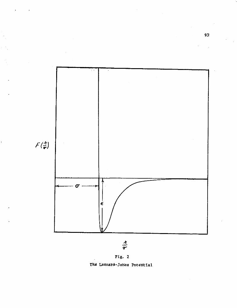
Fig. 2

94

and

For convenience we d e f i n e the dimensionless quan t i t i e s :

(5.1 - 3) 4 s - lr R a-

J*= - x 7 c

(5.1 - 4 )

(5.1 - 5)

(5.1 - 6 )

(5.1 - 7)

(5.1 - 8)

These reduced v a r i a b l e s a r e convenient s ince only one ca l cu la t ion f o r

t h e corresponding states of a series of gases i s then necessary.

Since, i n general , t h e p o t e n t i a l i s not purely repuls ive , bound

states are possible . A t yp ica l pseudo-potential f o r a p a r t i c u l a r

angular momentum and energy is shown i n Fig. 3. Depending on t h e

ezergg a d rrngular momentum, t h e r e can be one, two o r t h ree turn ing

poin ts ,

is below t h e zero of energy and the energy i s negat ive.

tu rn ing poin ts on a bound t r a j ec to ry .

Two tu rn ing poin ts a r i s e when t h e well i n the pseudo-potential

These a r e

For energies , above zero,

95

Fig. 3 2 f 0%

h* 2 The Pseudo-potential / - ( d l + - d

/L for an Orbiting Angular Momentum

96

t he outermost tu rn ing point i s always on a non-bound t r a j e c t o r y .

When t h e r e are t h r e e turn ing points, t h e energy and angular momentum

do not uniquely spec i fy a s ing le t r a j ec to ry . However, every choice

of b and J corresponds t o one and only one non-bound t r a j e c t o r y .

Most of t h e d iscuss ion of Sec. 2 . 6 holds f o r t h e non-bound tra-

j e c t o r i e s of any po ten t i a l . I n t he manner given the re , w e can def ine

the q u a n t i t i e s and 8 e The s p e c i f i c coordinate systems f o r

t hese q u a n t i t i e s which were discussed i n Sec. 2.6 a r e s t i l l va l id .

Further , t he i d e n t i t y equation (2.6 - 18) holds; and w e can i n t e g r a t e

over t h e non-bound por t ion of t he pos i t ion-ve loc i ty space by

i n t e g r a t i n g over 5 4 , 3’)

/ /

/

For purely repuls ive po ten t i a l s , t he s c a t t e r i n g angle ,d i s

always pos i t i ve . For a general p o t e n t i a l t h i s i s not t r u e , A

phenomona known as near o rb i t i ng occurs when theenergy and angular

momentum are such t h a t t he energy i s approximately equal t o t h e

maximum i n t h e pseudo-potential . Under these condi t ions t h e p a r t i c l e

o r b i t s t h e s c a t t e r e r a number of t imes; and t h e s c a t t e r i n g angle

i s l a r g e and negative. I f the energy is s l i g h t l y g r e a t e r than t h e

p o t e n t i a l maximum, t h e r a d i a l v e l o c i t y of an incoming p a r t i c l e f a l l s

nea r ly t o zero; but remains negative as t h e r a d i a l s epa ra t ion

approaches the m a x i m u m of the pseudo-potential . The p a r t i c l e thus

t r a v e l s i n a nea r ly c i r c u l a r o r b i t wi th a s l i g h t inward spiral .

Depending on how c lose t h e incoming energy i s t o t h a t of the

p o t e n t i a l maximum, the p a r t i c l e may make seve ra l such o r b i t s . F ina i iy ,

t h e p a r t i c l e s p i r a l s i n over t h e maximum, and t h e r a d i a l v e l o c i t y

decreases then increases sharply t o zero a t t he turning poin t ,

91

I

The radial v e l o c i t y then becomes p o s i t i v e and t h e p a r t i c l e s p i r a l s

outward on a t r a j e c t o r y symmetric t o t h e incoming t r a j e c t o r y . If

t h e incoming p a r t i c l e has energy s l i g h t l y less than the maximum i n

the pseudo-potential , t h e p a r t i c l e undergoes a s i m i l a r type of

o r b i t i n g but does not pass over t he maximum. Near o r b i t i n g presents

no t h e o r e t i c a l d i f f i c u l t i e s ; but computationally i t introduces

d i f f i c u l t i e s because t h e s c a t t e r i n g angle and the dura t ion of a

c o l l i s i o n a r e very large. 11

The t r anspor t c o e f f i c i e n t expressions of Snider and Cur t i s s

have been w r i t t e n i n terms of f i v e bas i c i n t e g r a l s over t he two

p a r t i c l e posr t ion v e l o c i t y space by Snider and McCourt 35

(Only

t h r e e of these i n t e g r a l s comprise p a r t of 8: , 8; and

* c& . The o the r two give por t ions of C A and C*r, One

of t hese i n t e g r a l s i s c lose ly r e l a t e d t o $/g : # u// e)/&/ which, as w e have shown, a r i s e s i n the s o l u t i o n of the i n t e g r a l

equat ions. The o ther four i n t e g r a l s a r i s e i n the eva lua t ion of t h e

f l u x vectors . Our treatment leads t o an add i t iona l i n t e g r a l , A' . The f i v e bas i c i n t e g r a l s i n t h e Snider and Cur t i s s treatment

have been evaluated f o r t he Lennard-Jones p o t e n t i a l by Curt iss ,

McElroy, and Hoffman . These i n t e g r a l s over t h e non-bound state 36

regions of t he two p a r t i c l e pos i t ion-ve loc i ty space are evaluated

by f i r s t transforming t o the reduced va r i ab le s mentioned previously.

The in t eg ra t ions over the t h r e e angles which determine t h e p lane of

c o l l i s i o n and i t s o r i e n t a t i o n i n t h e plane can be c a r r i e d out

immediately. The remaining v a r i a b l e s determine a t r a j e c t o r y i n t h e

c o l l i s i o n plane and a point on t h e t r a j e c t o r y .

are c a r r i e d out i n t h e ('4 < f*) coordinate system, the- remaining

I f t h e i n t e g r a t i o n s

98

t h ree in t eg ra t ions are over h* , and the angle te between

Fz* and -J*, . . By manipulating the d i n t eg ra t ions w e can transform t h e

i n t e g r a l s t o i n t e g r a l s only over t h e incoming port ions of t h e

t r a j e c t o r i e s . If w e represent t h e integrand of a t y p i c a l eP i n t e g r a l

by H(A#, j* ZP) , then the ZP i n t e g r a l is

J / q f A : p 9 > " ; " " dz. t r a j e c t o r y

T approach, tp s- t

7 , On t h e incoming por t ion of the

0

o ,L 2p d ' ; and a t t h e d is tance of c loses t

. We can wr i t e

f

c T 0

0 c z

and i s /r The i n t e g r a l i s over t h e domain of fl from o t o

thus an i n t e g r a l over t he incoming por t ion of the t r a j e c t o r y ,

i n t e g r and

The

I contains equal contr ibut ions from the point , d g j f l ! on

t h e incoming por t ion of t h e t r a j e c t o r y and t h e corresponding point

(through symmetry) ( A * , a", 2-ZQ ) on t h e outgoing por t ion

of t h e t r a j e c t o r y .

99

There a r e seve ra l choices of coordinates we can u s e t a ca r ry out

t he in tegra t ions over t h e incoming por t ion of the t r a j e c t o r y , A

convenient choice i s '1 , f4 and . The coordinates

and f spec i fy a t r a j e c t o r y and R s p e c i f i e s a point on the

+

7f + ?

incoming por t ion of t h i s t r a j e c t o r y . From equations (2 .6 - 2) and

(2.6 - 3) we note t h a t t hese coordinates have the advantage

numerically of spec i fy ing d* and j without t he necess i ty of

determining a root of an a lgeb ra i c equation. The i n t e g r a t i o n l i m i t s

on /I

*

x f are f* and i n f i n i t y . The in t eg ra t ion over [J'' and

f+ i s r e s t r i c t e d t o t h e non-shaded areas of t he f i r s t quadrant

i n Fig. 4 . The area A is excluded i n the i n t e g r a t i o n because

t h e r e the p o t e n t i a l energy a t rr exceeds t h e t o t a l energy, The

a rea 8 i s excluded because it corresponds t o bound s t a t e s . Poin ts

i n t h e in t eg ra t ion region which l i e near t h e boundary curve of ,8

correspond t o non-bound states wi th near -orb i t ing t r a j e c t o r i e s . Those

poin ts lying near t he pa r t of t he boundary curve wi th p o s i t i v e s lope ,

correspond t o c o l l i s i o n s where the p a r t i c l e energy i s s l igRtPy

g r e a t e r than the maximum i n t h e pseudo-potent ia l ; and those poin ts

ly ing near t he p a r t of t he curve with negat ive s lope, correspond t o

c o l l i s i o n s where the p a r t i c l e energy i s s l i g h t l y l e s s than t h e

pseudo-potential maximum. As mentioned previously, po in t s near t he

boundary curve of 8 present computational problems because the

angle of s c a t t e r i n g i s l a rge and the du ra t ion of the c o l l i s i o n i s long,

The Jacobian of t he t ransformation ( A * * ,y ) 3 (A", '9 11; P) J s J i s

100

23 Fig. 4

The integration Region for

101

(5.1 - 10)

To evaluate the determinant in equation (5 .1 - 10) w e make use of

the relations:

1

* = [(S‘JX L- / - / A * ) ] L (5.1 - 11)

(5.1 - 12)

(5.1 - 13)

which follow from equations (2.6 - 2 ), (2.6 - 3 ), (2.6 - 4 ) and

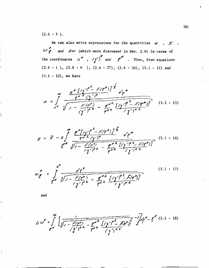
102

(2.6 - 5 ).

8

We can a l s o write expressions for the quantities cc , ,f , (which were discussed i n See. 2.6) i n terms of

* the coordinates h ?F , /]’I and

(2.6 - 1 ), (2.6 - 6 ), (2.6 - 27), (2.6 - 30), (5.1 - 11) and

(5.1 - 12), w e have

f+ . Then, from equations

7

b

00

J A4

and

(5.1 15)

(5.1

(5.1 - 17)

103

From See. 2.6 we have, on the incoming portion of a trajectory,

(5 .1 - 19)

4 -Cos& i'. ( 5 . 1 - 20)

(5 .1 - 21)

(5.1 - 2 2 )

and

On the outgoing portion of the trajectory,

(5 .1 - 23)

( 5 . 1 - 24)

( 5 . 1 - 25)

(5 .1 - 26)

(5 .1 - 27)

( 5 . 1 - 28)

I O U

We now reduce the integral J*/, - LJI d& t o a form

which i s convenient for computation, From equation ( 3 . 1 -12) we

have

If we make t h e variable transformation

which was discussed i n Sec. 3 . 6 , then the f i r s t integral i n

equation ( 5 . 1 - 29) i s zero by Gauss’ theorem. Thus,

, lit/. ) -4 ( 2 , c)

105

The quan t i ty is given by

(5.1 - 31)

There is no con t r ibu t ion t o

z -

/ / k .' fi @/)dM from t h e term 4

r p by v i r t u e of t h e gradient . Also, t he terms

and - f $ do not con t r ibu te a f te r i n t e g r a t i o n over r /

z - 2 - w

t h e angles of . Hence, c

(5.1 - 32)

In t eg ra t ing over y i e lds

I n t h e manner previously discussed, t h i s expression f o r

r( J = : .&, e/)/@, can be transformed t o an i n t e g r a l over t h e

I f we use as i n t e g r a t i o n va r i ab le s the incoming t r a j e c t o r i e s . + 4

coordinates A* , '.) and 6 , we have d

106

The integrand of t h e i n t e g r a l i n equation (5 .1 - 34) is a funct ion * + -# of t h e reduced q u a n t i t i e s A , 9’1 , .f and 7* only. The

var ious func t iona l r e l a t i o n s necessary t o w r i t e t h e integrand i n

t h i s form a r e given by equations (5 .1 - 10) - (5 .1 - 28). The i n t e g r a l

i t s e l f i s a funct ion of only ,7# and i s appl icable t o t h e

corresponding s ta tes of a series of gases.

The other four i n t e g r a l s bas i c t o t h e r e s u l t s of Snider and

C u r t i s s can be reduced t o a convenient computational form i n a

similar manner.

were performed are discussed i n d e t a i l by 36

Hoffman .

The numerical methods by which these i n t e g r a t i o n s

Curt iss , McElroy and

The i n t e g r a l 4 which arises i n our treatment can be reduced

t o a computationalhrmin a similar manner, We f i n d t h a t r ?

t r a j e c t o r y I 4 / 4 A f 4 “ / A ‘ E A” )‘J *J incoming .’+ f 7 * /p 7)outgoing t r a j ect ory

The func t ion 3 ( &*-J 1) which appears i n t h e integrand

i s i t s e l f an i n t eg ra l . From equation ( 2 . 8 - la, we have

We can w r i t e t h i s i n t e g r a l i n confocal e l l i p t i c coordinates and

perform t h e t r i v i a l angle in t eg ra t ion t o obta in

I f w e then introduce t h e va r i ab le change

and

w e ob ta in

The i n t e g r a l 4 can be

(5.1 - 38)

(5.1 - 39)

computed numerically from t h i s expression

and equat ion (5.1 - 35).

107

Sect ion 5.2 Numerical Evaluation of 8 We s$e, from equations (5.1 - 35) and (5,1-- 4 0 ) , t h a t i s

a f ive - fo ld i n t e g r a l ,

i s d i f f i c u l t because t h e time required (on even a l a r g e computer)

i s p roh ib i t i ve ly long, We,therefore, examine an approximate technique

Straightforward numerical i n t e g r a t i o n of

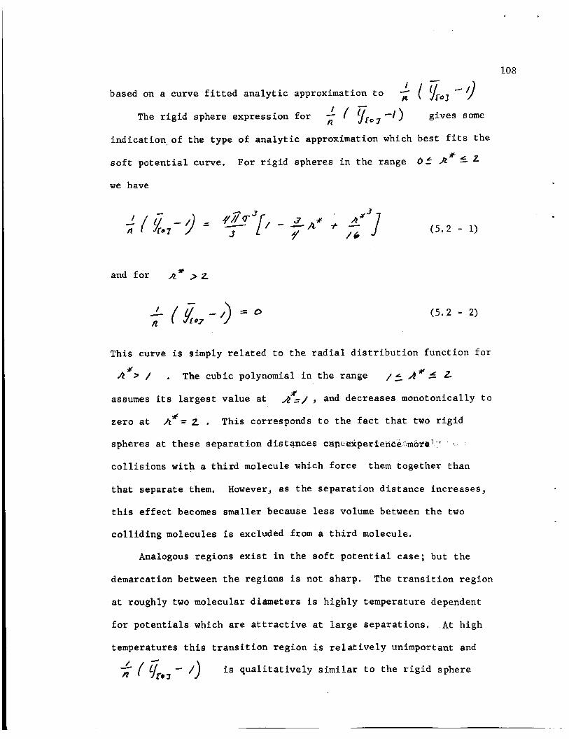
based on a curve fitted analytic approximation to ( go, - 9 I

The rigid sphere expression for - yro7 - 1 ) gives some n indication of the type of analytic approximation which best fits the

soft potential curve.

we have

For rigid spheres in the range O f A* f

and for A* > 2

( io, -1) = * n

(5.2 - 1)

(5.2 - 2)

103

This curve is simply related to the radial distribution function for # R > / , The cubic polynomial in the range / f R * 4 t

x assumes its largest value at A = / , and decreases monotonically to

zero at

spheres at these separation distances capceiperienCe~mor8''r

collisions with a third molecule which force them together than

that separate them, However, as the separation distance increases,

this effect becomes smaller because less volume between the two

colliding molecules is excluded from a third molecule,

A"= 2 , This corresponds to the fact that two rigid

1

Analogous regions exist in the soft potential case; but the

demarcation between the regians is not sharp. The transition region

at roughly two molecular diameters is highly temperature dependent

for potentials which are attractive at large separations, At high

temperatures this transition region is relatively unimportant and

- /) is qualitatively similar to the rigid sphere

109

curve. The molecular s i z e is r e l a t i v e l y smaller, however, due t o

t h e increased penet ra t ion of two molecules i n a high energy c o l l i s i o n .

A t lower temperatures, t h e r e i s a maximum i n the curve a t roughly two

molecular diameters.

neares t neighbors.

sphere curve because the re i s no a t t r a c t i o n t o favor t h i s separa t ion .

This is due t o t h e favorable packing of second

There is no analogous m a x i m u m i n t h e r i g i d

For the purpose of curve f i t t i n g , t h e func t ion - was ca lcu la ted f o r the Lennard-Jones p o t e n t i a l a t f i v e widely

separated temperatures and for a number of separa t ion d is tances .

The ca l cu la t ions were carried out on a CDC 1604; about 3-1/2 minutes

being required f o r a given temperature and separa t ion d i s t ance , The

ca lcu la ted r e s u l t s are given i n Table 1. Included a l s o ( i n

parentheses) a r e a number of values obtained by de Boer and Michels . These r e s u l t s a r e i l l u s t r a t e d i n Fig, 5. For comparison, t he r i g i d

sphere curve i s a l s o given.

n ’ v 3 1 (Jrq -11

37

The integrand of the i n t e g r a l heavi ly weights t h e region

of 4% between one and two molecular diameters. For smaller

values of A% , zero ; f o r l a r g e r

t h i s e f f e c t . It

- F/..*I t h e f a c t o r 7* makes t h e integrand e f f e c t i v e l y

x values of A t h e gradient of t he p o t e n t i a l has

is, therefore , most important t o accura te ly curve

-17 i n the region of h -# between one and two

molecular diameters. The funct ion can be well f i t t e d i n t h i s region

by a cubic polynomial.

behavior i s reasonable. For values of exceeding tm mslecular

diameters the func t ion I .v3

with increas ing A* . This decay t o zero i s approximated (purely

empir ica l ly) by an exponential funct ion. As discussed previously,

From our r i g i d sphere ana lys i s , such a

*

- /7 undergoes a decay t o zero

1 10

TABLE I

.

R* . 4

. 5

. 6

. 7

.8

. 9

1.0

1.2

1.4

1.6

1.8

2.0

2.2

2.4

2.6

2.8

3.0

3.2

3.4

3.6

3,8

3.1623

2.3259

1.6688

1.1592

0.1977

1.0221

0.6948

0.4513

0.2929

0.1927

0.1290

0.0880

0,0611

(1.652)

(1.204)

(0.480)

(0.182)

(0.178)

(0.423)

(0.886)

(1,211)

(0,999)

(0.281)

1.2064

0.8225

(0.501)

(0.237)

(-0.147)

(-0.362)

(-0.425)

(-0.329)

(-0,103)

(-0.080)

0.1168 ( 0.134)

( 0.092)

0.0676 ( 0.065)

( 0.046)

0.0313

0.0213

1.2051

0.9693

0.7547

0.5617

0.2423

0.0167

-0.1075

-0.1230

-0.0708

-0.0313

-0.0135

-0.0062

-0.0031

-0.0017

-0.0010

-0.0007

1.4183

1.2108

1.0134

0.8285

0.6576

0.5024

0.2445

0.0661

-0.0215

-0,0294

-0.0167

-0,0085

-0.0045

-0.0025

-0.0015

-0.0009

1.2472

1.0754

0.9084

0.7496

0.6013

0.4655

0.3438

0.1496

0.0313

-0,0068

-0.007 1

-0.0039

-0.0021

-0.0011

-0,OQG7

-0,0004

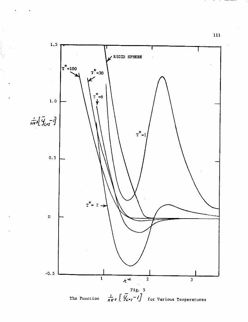
111

1, I

1.0

0.5

0

-0.5

h. I I

RIGID SPHERE

I I I 1 iZcL 2 3

Fig. 5

The Function =a YLO,-/] f o r Various Temperatures -

I

112

t h e r e is a t r a n s i t i o n region which is h ighly dependent on temperature

between t h e range of a p p l i c a b i l i t y of t hese t w o approximations.

This t r a n s i t i o n region is more important a t low temperatures than

a t high temperatures; but even a t low temperatures t h e con t r ibu t ion

t o R i s small. The curve f i t t e d approximations a t t h e var ious

temperatures are given i n Table 2.

The numerical eva lua t ion of t h e c o l l i s i o n a l cont r ibu t ions t o

t h e t r anspor t v i r i a l coe f f i c i en t has been discussed i n d e t a i l by

36 Cur t i s s , McElroy, and Hoffman . The computational problems

involved i n eva lua t ing the i n t e g r a l 4 a r e q u i t e s imi l a r t o

those encountered i n t h e earlier study.

Sect ion 5.3 Numer'ical' Va'lui3 of' the ' Redu'c'ed' TtanSport' V i r i a l

Coeff i c ' i en t s . From equations (4 .2 - 21) and (4.2 - 22) we have

;Y

This quan t i ty along with f b ; ) s . c , and ( )s. c ,

by Cur t i ss , McElroy and Hoffman ) , and 8; and dA a re 36 *

( 5 . 3 - 1)

(as given

given i n n(2 ,a* L

Table 3. The values of a r e taken from Molecular

38 Theory'of Gases and LiquSds by Hirschfelder , Cur t i s s and Bird . The tabula ted q u a n t i t i e s a re i l l u s t r a t e d i n Figs . 6 and 7 .

Althaugh CiirtissJ McElroy and Hoffman considered r igorous ly

only the c o l l i s i o n a l cor rec t ions t o t h e t r anspor t v i r i a l c o e f f i c i e n t s ,

they cor rec ted t h e i r results i n an i n t u i t i v e manner t o account f o r

t h r e e body in t e rac t ions . The co r rec t ion i s based on a method

113

T* - 1

2

8

30

100

0 - 2.0

2.0 - 2.6

2.6 - 00

0 - 2.0

2.0 - 00

0 - 1.8

1.8 - 2.0

2.0 - Qo

0 - 1.6

1.6 - 1.8

1.8 - oo

0 - 1.5

1.5 - 1.8

1.8 - 00

3

3

* 2

2 11.657 - 17.603r* + 8.1347r* - 1.0122r

-129.75 + 164.00r - 67.872r + 9.2667r * * *

* 190,64exp(-2,1594r )

5.1084 - 7.5927r + 2.9521r - ,22929r

1

3 * 2 * * .1 - 6.2996

(r*-l .8) (r*-l , 8) (11.864 + 8.2291

* 1 +. 79720 (r*-1.8)3 exp(-l .9241r )

2 3 * * 3.3345 - 3.5777r 4- ,66075r + .14427r*

* -. 59320 + ,26120r

-248.43kxp (-4.08 16r ) *

2 3

2

* 2.5863 - 2.4615r + .14083r* + .23685r*

.64644 - ,93865r + .32867r * *

* -7.5857exp(-3.0859r )

2 3 + .26942r*

* 2.0038 - 1.9103r - .019016r*

2 1.0899 - 1.2932r + .37987r

* * *

-1.5087exp( -2.9777r )

114

T*

TABLE 3

1 2 8 30 100

VALUES OF THE SECOND V I R I A L COEFFICIENTS FOR VISCOSITY

AND THERMAL CONDUCTIVITY

0.6942

3.0513

0.8991

1.6967

0.6827

1.1169

0.5156

0.8008

-1.226 -0.3512 -0.7737 -0.7a04 -0.6487

0.3430 0.1254 -0.0977 -0.1331 -2.439

3.440 2.7001 0.9230 0.3365 0.1521

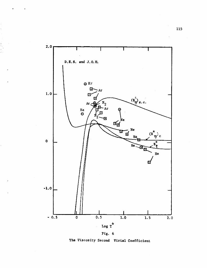
115

2. c

1. c

0

-1, a

D.E.S. and J . O . H .

I 0 Kr

I

* Log T

Fig, 6

The Viscosity Second Virial Coefficient

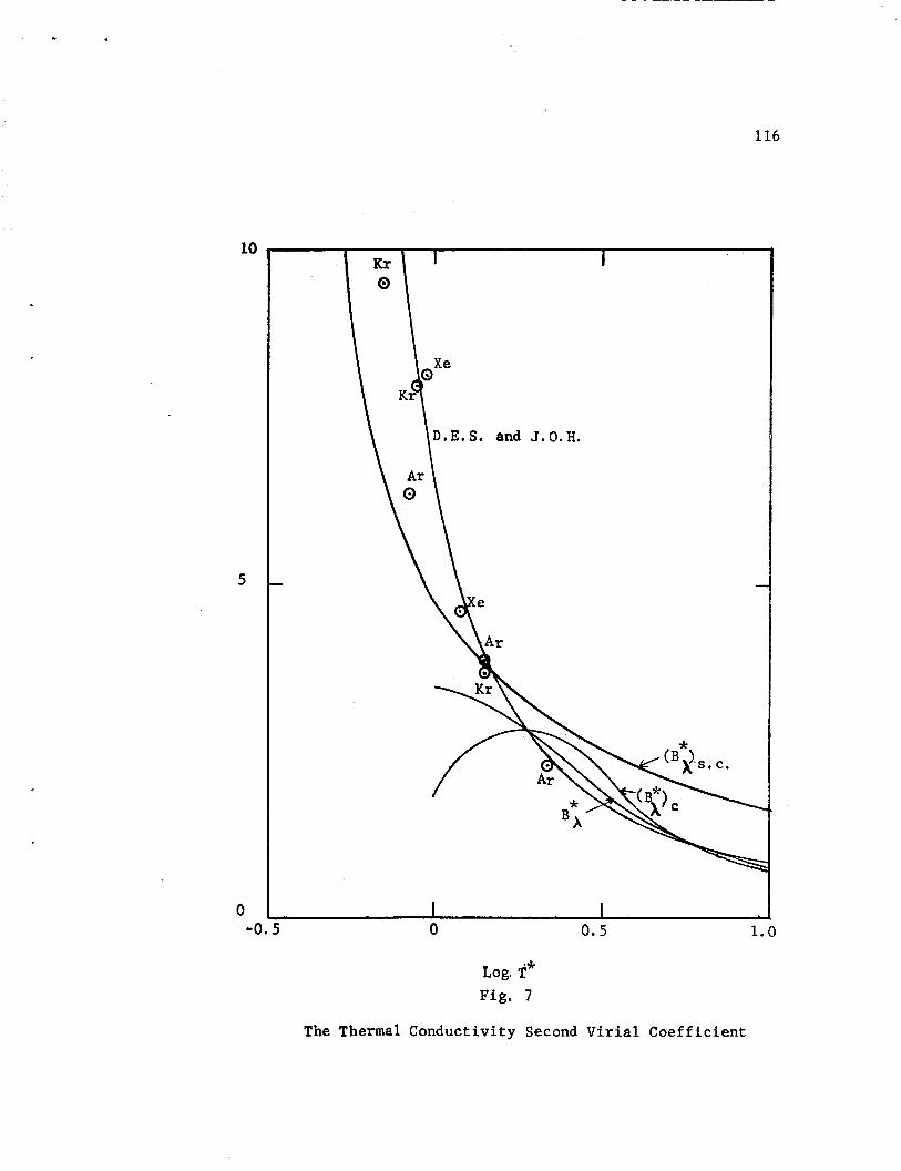
116

10

5

0 4

and J. 0. H.

5 0 0 . 5 1.0

Log. T* Fig. 7

The Thermal Conductivity Second Virial Coefficient

1 1 7

suggested by Enskog f o r t h e approximate app l i ca t ion of h i s work on

the r i g i d sphere gas t o a realist ic system. The i r corrected

c o e f f i c i e n t s are included i n the f igu res , and are labeled (B;Ic and f a;)c . Also i l l u s t r a t e d i n t h e f i g u r e s are the r e s u l t s of

6

12 a theoretical s tudy by Stogryn and Hirschfe lder on the e f f e c t of

s t a b l e and metastable bound molecular p a i r s on t h e t ranspor t v i r i a l

coe f f i c i en t s .

Experimental po in ts from two sources a r e included i n the f igu res .

The c i r c l e d poin ts a r e taken from t h e paper by Stogryn and Hirschfelder .

The v i s c o s i t y poin ts i n squares a r e recent values given by Flynn,

Hanks, L e m a i r e and Ross3’. The parameters used t o reduce t h e i r values

t o corresponding s t a t e s values a r e given by Cur t i s s , McElroy and

36 Hoffman ,

.y. Experimentally, as a funct ion of i s l a rge and

4 pos i t i ve a t low 7 . i s increased, t he value decreases and

, .+ becomes negat ive. The shape of t h e dA curve i s s imi l a r a t l o w

temperatures; but, due t o a lack of da ta , it can only be extrapolated

a t high temperatures.

Both t h e o r e t i c a l curves f i t t h e d a t a reasonably w e l l a t high

i s negat ive a t high temperatures O;

temperatures. I n p a r t i c u l a r ,

and approaches zero asymptotically from below. This i s i n c o n t r a s t

with the i n t u i t i v e l y obtained quan t i ty (G)c. which approaches zero

from above. The dev ia t ion between theory and experiment a t low

x

I

temperatures i s probably Siie t~ t he effect of bound s t a t e s which

have not bee.n t r ea t ed i n a s a t i s f a c t o r y t h e o r e t i c a l manner.

118

The purpose of t h i s s tudy i s t h e i n v e s t i g a t i o n of t he dens i ty

expansions of t h e t r anspor t coe f f i c i en t s . We do t h i s by formally

consideringthe equations which govern t h e t i m e evolut ion of the

lower order d i s t r i b u t i o n func t icns . This approach leads u s t o a

de r iva t ion of a mod'ified or generalized Boltzmann equation which

includes t h e e f f e c t of t h r e e body in t e rac t ions . From t h e so lu t ion

of t h i s equation, w e ob ta in expressions f o r t he t r anspor t c o e f f i c i e n t s .

I n Chapter I1 w e develop a f a c t o r i z a t i o n p r i n c i p l e which i s a

general izat ion of t h e Iisual molecular chaos assumption,

p r inc ip l e i s used t o approximate t h e 1.4 +I) order d i s t r i b u t i o n

funct ion i n terms of the A lower order d i s t r i b u t i o n funct ions.

This ?!&

We truncate t h e B.B.G,K.Y. hierarc:.hy by t h e use of t h i s approximation.

The t runcat ion r e s u l t s i n a closed but coupled system of equations

f o r t h e k, lower order d i s t r i b u t i o n functions. W e compare t h i s

set of equations with the formal expansion of t h e Boltzmann equation

given by Hollinger and Cerciss e

10

The Hollinger and Cur t i s s exparsion of t h e Boltzmann equation

i s based orr a formal s o l u t i a n f o r

expression f o r f hihen subs t i t u t ed i n t o t h e B. B. G, K. Y.

/ ") i n terms of f ''I . This Tz -l

equation, y i e lds a Boltzmann equation whose c o l l i s i o n i n t e g r a l i s

given as a s e r i e s expansion. The f i r s t term i n t h e expansion gives

rise t o the ordirrary c o l l i s i o n i n t e g r a l p lus the c o l l i s i o n a l

7 co r r ec t ions suggested by Green . The second t e r m i n the expansion

of t h e c o l l i s i o n i n t e g r a l desc r ibes th ree body c o l l i s i o n a l e f f e c t s .

119

This term involves t h e dynamics of two and t h r e e body c o l l i s i o n s i n

a very complex manner.

term a l s o arises when t h e B . B . G . K . Y . hierarchy is terminated by t h e use

off7the f a c t o r i z a t i o n p r i n c i p l e f o r

We show e x p l i c i t l y t h a t t h i s t h r e e body

Our approach d i f f e r s from t h a t of Hollinger and Curt iss , however,

i n t h a t w e do not formally solve t h e /‘*hquation. Instead w e

consider t h e / and / equations simultaneously. We approximate

t h e s o l u t i o n of t h e 1

f /I (2 1

f z> equation t o de r ive a Boltzmann equation

h i c h takes i n t o account t h r e e body i n t e r a c t i o n s i n an approximation.

For t h e s p e c i a l case of r i g i d spheres, t h i s equation reduces t o the

Enskog dense gas equation. The Boltzmann equation derived i n t h i s

manner does not depend i n d e t a i l on the dynamics of t h r e e body

c o l l i s i o n s , This equation i s so1ved;and from t h e s o l u t i o n expressions

f o r t h e t r anspor t c o e f f i c i e n t s are derived as dens i ty expansions.

The l i n e a r terms i n t h e dens i ty expansions contain sepa ra t e

c o l l i s i o n a l and t h r e e body contr ibut ions. The c o l l i s i o n a l contribu-

t i o n s have been considered previously by Snider and Cust iss 11 . The

t h r e e body contr ibut ions a r e new t o t h i s work.

These r e s u l t s apply only t o t h e non-bound s t a t e con t r ibu t ions

t o t h e t r a n s p o r t coe f f i c i en t s . Bound states have not y e t been

handled properly i n a t h e o r e t i c a l manner; t h e app l i ca t ion of t h e

present formalism t o t h i s problem w i l l be considered i n a l a t e r

study. 36

Receatly Cur t i s s , McElroy and Hoffman have ca l cu la t ed t h e

c o l l i s i o n a l con t r ibu t ions t o t h e t r anspor t c o e f f i c i e n t s of a gas

of molecules, which i n t e r a c t according t o a Lennard-Jones p o t e n t i a l .

120

In Chapter V we complete these results by calculating the three body

collisional contributions. The theoretical results are compared with

experimental values.

.

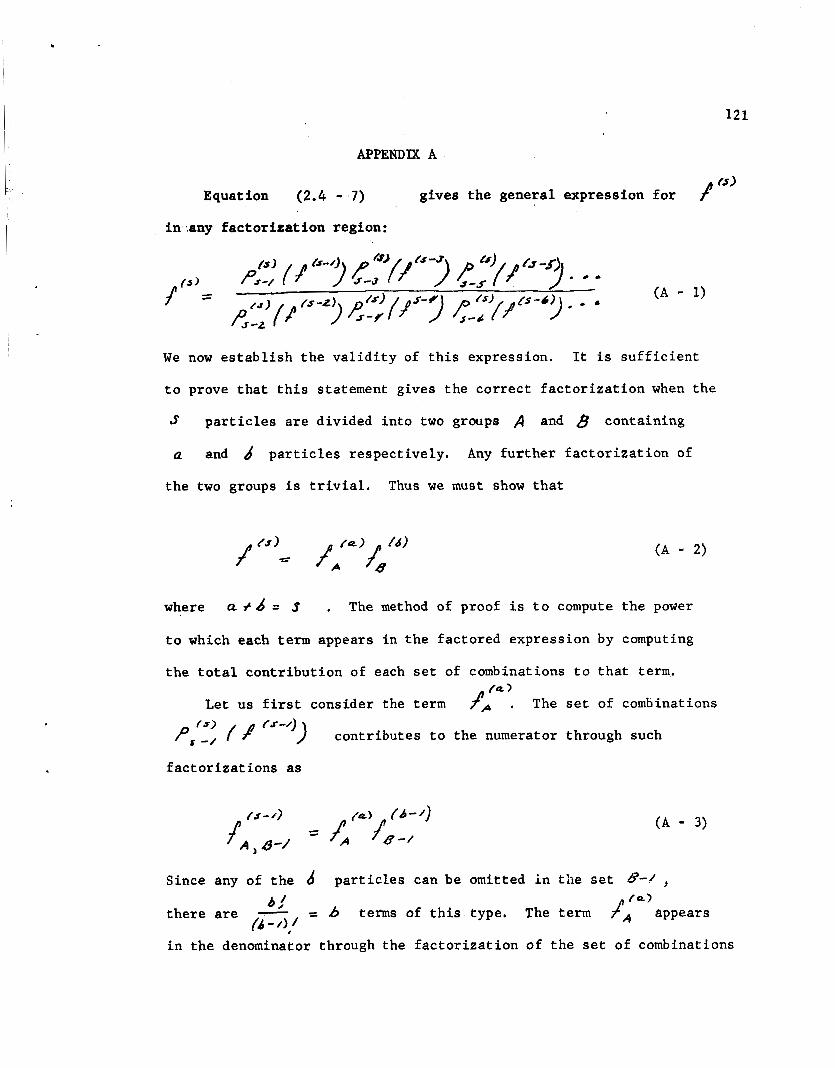
12 I

APPENDIX A

Equation (2.4 - 7) gives t h e general expression f o r

i n . any f a c t o r i z a t i o n region:

We now e s t a b l i s h t h e v a l i d i t y of t h i s expression.

t o prove t h a t t h i s statement gives the co r rec t f a c t o r i z a t i o n when t h e

S p a r t i c l e s a r e divided i n t o two groups A and 8 containing

Q and d p a r t i c l e s respec t ive ly . Any f u r t h e r f a c t o r i z a t i o n of

It is s u f f i c i e n t

t h e two groups is t r i v i a l . Thus w e must show t h a t

where cz + d = S . The method of proof i s t o compute the power

t o which each term appears i n t h e fac tored expression by computing

t h e t o t a l con t r ibu t ion of each s e t of combinations t o t h a t term, /Q 1

L e t us f i r s t consider the term f p . The set of combinations

cont r ibu tes t o the numerator through such -/

f a c t o r i z a t i o n s as

Since any of t h e d p a r t i c l e s can be omitted i n the set L?-/

t he re a r e - b,/ b terms of t h i s type. The term fA‘L’appears (d-1) 1

i n t h e denominator through the f a c t o r i z a t i o n of t h e set of combinations

.

122

. Such a f a c t o r i z a t i o n i s

There a re ,-- b ! 4 - 4 f4-4 d i f f e r e n t poss ib le /@ a - r /4-z1 . {4 -2I.l ! z

By continuing t h i s reasoning t o show t h e successive cont r ibu t ions of

e:;’( f’ -7 J . P J-7’( lS? /J t cs-u)’ 1 , e t c . , we f ind t h e

power, R A , t o which f,”’ i s r a i sed i n t h e fac tored expression i s

But s ince

it follows t h a t

S i m i l a r reasoning shows t h a t

no - / (A - 8) /a -/>

I n a s imi l a r manner we f ind t h a t any term of the t y p e -, b. /

A! a,/ appears i n t h e numerator - = / times from t h e f a c t o r i z a t i o n of

the combination set pa,, ‘’) { $‘*-‘)) . The set 4:’ [ / c s - z ’ )

cont r ibu tes i n the denominator A ! = b times, Continuing

t h i s reasoning w e f ind t h e power (b-/j , / //

t o which any term of t h e

a # * In an analogous manner w e establ ish that for

and, therefore,

123

(A - 10)

(A - 11)

124

APPENDIX B

I n t h i s appendix, w e evaluate t h e i n t e g r a l s f (5 : u) Ix / , zB/& s

and

equat ions,

](x .! _U) M/, ' / ~ which arise i n t h e s o l u t i o n of t h e i n t e g r a l - -

L e t us consider t he i n t e g r a l ][z:g) Lt/lEdW/ - . From the - - d e f i n i t i o n of -7 g i v e n by equation (3 .1 -Q , w e have - -

>

where 4 and are r e l a t e d t o W, d and Nz d by t h e equations

By Gauss theorem w e have

125

where w e have made use of the relat ion

2 The quantity i s given by

We can integrate over to yield

From the identity of equation ( 2 . 6 - 18) we have

Hence

or equivalently

12 6

In the f irst integral i n equation ( B - 10) w e make the coordinate

and write c A / i n the particular 1

transformation ( 4 ~ 4 ) 4 ( Y , A / )

coordinate system discussed i n Sec, 2;6. We then have

We can integrate over 4 t o y ie ld

(B - 12)

and

.

127

Hence

(B - 15)

The second virial coefficient, 8 , is given by

Thus, we have

(8 - 16)

(B - 17)

By an analogous integration procedure we find that

( B - 18)

128

and, thus, the integrals $/<:g) M/,'B/bi$ and j ( g :g) can be written in terms of the second virial coefficient,

its temperature derivatives.

- - L - e

, and

c

BIBLIOGRAPHY

129

S.' Chapman and T. G. Coding, The Mathematical Theory of Non-

uniform Gases (Cambridge University Press, London, 1960),

L. S. Ornstein, dissertation, Leiden, 1908.

L. Boltzmann, Wien. Ber. 66, 275 (1872).

S.'Chapman, Phil. Trans. Roy. S0c.A 216, 279 (1916).

2

3

D, Enskog, dissertation, Upsala, 1917.

D. Enskog, Svensk. Akad, Handl. 63, No. 4 (1922).

H. S. Green, NoIeCu'lw The'ottr' bY' Flh'id's', (North Holland Publishing Co.,

Amsterdam, 1952).

N. N. Bogolubov, J. Phys. (U.S. S . R . ) 10, 256 (1946).

N. N. Bogolubov, Problemv Dinamicheskoi Teorii v Statistichestoi

- Fizike, (Technical Press, MOSCOW, 1946).

9

lo H. B. Hollinger and C. F. Curtiss, J. Chem. Phys. 33, 1386 (1960).

R. F. Snider and C. F. Curtiss, Phys. of Fluids 1, 122 (1958). -

l2 D. E. Stogryn and J. 0. Hirschfelder, J. Chem. Phys. 31, 1531 (1959); I

33, 942 (1960).

M. Born and H. S. Green, A General Kinetic Theory of Liquids

(Cmhridge University Press, New York, 1949).

l4 J. G. Kirkwood, J. Chem. Phys. 14, 180 (1946).

l5 J. Ytron, Actua'l'ities Scientifiayes et Industrielles, Hermann and Cie,

-

Paris (1935).

P 30

BIBLIOGRAPHY (cont'd)

l6 G. E. Ifhlenbeck, The Boltzmann Bquation, University of Michigan publi-

cation, Navy Theoretical Physics (1957).

l7 S. T. Choh, dissertation, University of Michigan, 1958.

I8 M. S. Green, J. Chem. Phys. 25, 836 (1956). - M. S. Green, Physica 24, 393 (1958).

2o S. A. Rice, J. G. Kirkwood, J. Ross, and R. W. Zwanzig, J. Chem. Phys.

- 31', 575 (1959).

21 S . A. Rice, J. Chem. Phys. 31, 584 (1959). - 22 J , T. O'Toole and J. S. Dahler, J. Chem. Phys, 32', 1487 (1960).

2 3 J. S. Dahler, J. Chem. Phys. 30, 1447 (1959).

24 P. M. Livingston and C. F. Curtiss, Phys. of Fluids 4 , 816 (1961);

-

- P. M. Livingston,dissertation, Univessity of Wisconsin, 1961.

25 J. 0. Hirschfelder, C. F. Curtiss and R. B. Bird, Molecular Theory of

Gases and Liquids, (John Wiley and Sons, Inc., New York, 1954) p. 51,

26 H. Goldstein, Classical Mechanics (Addison-Wesley Publishing Co. , Inc.

Reading, Mass. ;1959), Chap. 8.

27 Ref. 26, p. .63.

28 Ref, 1, pp. 110-11.

29 Ref. 25, pp. 460-61.

30 Ref. 1, Sec. 7.51.

131

BIBLIOGRAPHY (cont 'd)

31 Ref. 1, Sec. 4.4.

32 Ref. 25, Sec. 7.A.

33

34

35

36

37

38

39

J. H. Irving and J. G. Kirkwood, J. Chem Phys. l8, 817 (1950).

R. F. Snider and C. F. Curtiss, Phys. of Fluids 3, 903 (1960).

R. F. Snider and F. R. McCourt, Phys. of Fluids 5, 1020 (1963).

C. F. Curtiss, M. B. McElroy and D. K. Hoffman, University of

Wisconsin Theoretical Chemistry Institute publication, WIS-TCI-46

(1964).

J, de Boer and A. Michels, Physicaz, 97 (1939).

Ref. 25. Table I - M G. P. Flynn, R. V. Hanks, N. A. Lemaire and J. Ross, J. Chem,

Phys. 38, 154 (1963).

-