MOLECULAR PHYSICS, 1993, VOL. 78, No. 3, 591-618

The Lennard-Jones equation of state revisited

By J. K A R L JOHNSON, J O H N A. Z O L L W E G and K EITH E. GUBBINS

School of Chemical Engineering, Cornell University, Ithaca, NY 14853, USA

(Received 8 July 1992; accepted 16 July 1992)

We review the existing simulation data and equations of state for the Len- nard-Jones (L J) fluid, and present new simulation results for both the cut and shifted and the full LJ potential. New parameters for the modified Benedict- Webb-Rubin (MBWR) equation of state used by Nicolas, Gubbins, Streett and Tildesley are presented. In contrast to previous equations, the new equa- tion is accurate for calculations of vapour-liquid equilibria. The equation also accurately correlates pressures and internal energies from the triple point to about 4.5 times the critical temperature over the entire fluid range. An equation of state for the cut and shifted LJ fluid is presented and compared with the simulation data of this work, and previously published Gibbs ensemble data. The MBWR equation of state can be extended to mixtures via the van der Waals one-fluid theory mixing rules. Calculations for binary fluid mixtures are found to be accurate when compared with Gibbs ensemble simulations.

1. Introduction

The Lennard-Jones 12-6 (LJ) potential is an important model for exploring the behaviour of simple fluids, and has been used to study vapour-l iquid and l iquid- liquid equilibria, melting, behaviour of fluids confined within small pores, small atomic clusters, a variety of surface and transport properties, and so on. It has also been widely used as a reference fluid in perturbation treatments for more complex fluids. In many ways, the LJ model is oversimplified [1]; for example, the form of the repulsive part of the potential is incorrect, being insufficiently repulsive at short distances, the C6 dispersion coefficient is too high while higher dispersion coefficients are neglected, and its application to dense systems neglects three-body forces completely. Nevertheless, it captures much of the essential physics of simple fluids.

There have been a number of attempts to fit simulation data for the LJ fluid to an analytical equation of state [2-12]. One of the most successful of these is the equa- tion of state of Nicolas et al. [5]. The Nicolas et al. equation of state uses a modified Benedic t -Webb-Rubin (MBWR) equation having 33 parameters, 32 of which are linear. This large number of adjustable parameters gives the equation sufficient flexibility to correlate data accurately over a wide range of state conditions.

The parameters for the Nicolas EOS were regressed from simulation data gen- erated by Nicolas et al. and by previous workers [2-5, 13-17], mainly from the late 1960s and early 1970s. By current standards, these data were, for the most part, for small systems and short run times. In addition, there were few vapour-l iquid equili- brium (VLE) data available, and the critical point of the LJ fluid was not known accurately. Nicolas et al. chose to constrain their equation of state to give critical density and temperature values of Pc = 0-35, and To* = 1-35, where p* = ( N / V ) ~ 3,

0026-8976/93 $10.00 �9 1993 Taylor & Francis Ltd.

592 J .K . Johnson et al.

N is the number of atoms, V is the volume of the system, tr is the LJ diameter, and T* = k T / e where k is Boltzmann's constant, T is the temperature in Kelvins, and e is the LJ potential well depth. These values lay within the older estimates of the critical properties given by Verlet [13]. Recent simulations show that Tc* = 1.35 is too high.

In recent years, the Gibbs ensemble Monte Carlo technique of Panagiotopoulos [18, 19] has proved particularly suitable for the direct determination of coexistence properties and for estimating critical points [20, 21]. Simulations in the Gibbs ensemble by several workers [18-20, 22, 23] have provided many more coexistence data for the LJ fluid, along with more reliable estimates for the critical temperature and density. The best current estimate of the critical point for the full LJ fluid predicted from Gibbs ensemble simulations is Pc = 0.304 + 0"006 and To* = 1.3164-0.006 [20, 21]. Lotfi et al. [11] have recently completed a study of the vapour-liquid coexistence properties of the pure LJ fluid by using isothermal- isobaric (NPT) ensemble simulations in conjunction with Widom's particle insertion method. Their data provide additional estimates of the critical properties as well as independent saturation densities and pressures. The data of Lotfi et al. are generally in very good agreement with the previous Gibbs ensemble results.

The Nicolas et al. equation of state does not accurately predict the saturation properties when compared with the recent Gibbs ensemble and Lotfi et al. data. Such discrepancies are particularly troublesome when using an equation of state for the LJ fluid as a reference term in perturbation theories of molecular fluids.

In this paper, we present new simulation data for the LJ fluid (section 2.2). These new data are used to refit the parameters in the MBWR equation (section 4). We do not use any VLE data in the fit, but we do constrain the parameters to give a critical density and temperature that agree with values estimated from the Gibbs ensemble and Lotfi et al. simulations. We demonstrate that the new parameters for the MBWR equation correlate accurately the simulation data, and that saturation vapour pressures and densities are predicted accurately when compared with recent simulation results.

2. Simulation data for the Lennard-Jones fluid

The full LJ potential is given by

I(;) (;;1 ~b(r) = 4e (1)

where e is the LJ well depth and ~r is the LJ atomic diameter. In computer simula- tions the potential must be truncated at some point r c < L/2 , where r c is the cutoff of the potential and L is the simulation box length. In practice, three types of truncated potential have been used: (1) cut potential (not shifted), (2) cut and shifted potential, and (3) cut and shifted force potential [24]. The cut and shifted force potential has the advantage in molecular dynamics (MD) simulations that there is no discontinu- ity in the potential or the force [5]. Corrections must be applied to the simulation results for each of these potentials in order to approximate the properties of the full LJ fluid. In each case, long range or tail corrections are computed by assuming that the pair correlation function is unity (g(r) -- 1) for r > r c. This leads to the following

The Lennard-Jones equation of state 593

0

0

~

~ 0

b..,, o

~.~

r ~

#.

b

"5 0

0

0

.0p .~ .op .~ . ~ .0p .'9 .~ . ~ .,.~ .op .~ . ~ ,.~ ~ c~ o o , - , o o o o . . . . . o , - , - o

I I I I I I I I I I I I I I I

~ o ~ o ~ m o . . . .

~ a a I ~ I I g ~ I I ~ ~ e ~ "

%

~ooo~ oo ~ o~-% ~ - . . . . ~ ~ o x ~ x ~ x

0

8 4~

~ ~ ~ ~ ~ ~;~ A ~

I::i

S o

,..~= , . s

O , 4 b

~ 2 ~: .,...,

0

",.e s

594 J . K . Johnson et al.

tail corrections for the pressure Pl~c and internal energy Ul~c [24],

32 0,2 tr 9 3 2 a 3

Ulr c = ~ np re re

In the vast majority of cases the LJ data published in the literature have made use of these long range corrections.

2.1. Literature data

Wood and Parker [25] at Los Alamos National Laboratory were the first to publish properties of the 3-dimensional LJ fluid from computer simulations. Since that time, many other authors have also performed simulations on the LJ fluid and published their findings. In table 1 we summarize the simulation results for much of the work on the thermodynamic properties of the LJ fluid. These include the follow- ing works: Wood and Parker, 1957 [25]; Verlet, 1967 [13]; Wood, 1968 [26]; Levesque and Verlet, 1969 [2]; Hansen and Verlet, 1969 [14]; Hansen, 1970 [3]; McDonald and Singer, 1972 [4]; Adams, 1975, 1976, and 1979 [16, 17, 27]; Nicolas et al., 1979 [5]; Nakanishi, 1986 [28]; Adachi et al., 1988 [8]; Shaw, 1988 [29]; Saager and Fisher, 1990 [30]; Lotfi et al., 1992 [11]; and Miyano, 1992 [12]. We note that Verlet and Weis [15] reported in 1972 previously published simulation results of [2, 3, 14], and augmented these data with either internal energy values or additional data points that were not reported in the original sources.

2.2. Simulation data from this work

We have performed simulations of the LJ fluid using both the MD and MC techniques. The bulk of the data are from MD simulations and are presented in table 2. For these simulations we used the cut and shifted potential ~bcs(r ) given by

(~b(r) - 4)(rc) if r < rc ~bcs(r)= 0 i f r > r c. (4)

We used a system size of 864 atoms and a cutoff of rc = 4"0a. Because of the large cutoff we expect any effect due to the discontinuity of the force at r c to be negligible. The full potential energies and pressures were recovered by adding back the poten- tial shift and applying the standard long range corrections given by equations (2) and (3). Vogelsang and Hoheisel [31] have used Baxter's continuation method to study the effect of the cutoff on thermodynamic properties. They found that for r c >_ 4.3a the normal long range corrections are practically exact for conditions close to the triple point. At higher temperatures or lower densities the effect of the cutoff is expected to be even smaller. We have compared our simulation results with data from very accurate simulations of Thompson [32] for a system of 1372 LJ atoms with the same cutoff. These independent data serve as a check of our coding and simulation technique. We found the agreement to be excellent. The temperature range covered in the simulations was 0.7 < T* _< 6.0. This covers a range from about the triple point (Tt*p ~ 0.69) to four and a half times the critical temperature (Tc* ~ 1.31). The densities ranged from 0.1 <_ p* <_ 1-25 at the highest temperature,

The Lennard-Jones equation of state 595

Table 2. Molecular dynamics simulation results of this work. The numbers in parentheses are the estimated errors of the mean in the last decimal place, e.g,, 8.51(2) = 8.51 -4-0-02.

p* T* P* U* Pc*s Uc~ Steps 6t*

0-1 6.0 0.6499(6) -0.478(2) 0.6525 -0.452 30000 0.002 0.2 6.0 1.442(1) -0-942(2) 1.452 -0-890 30000 0-002 0'3 6.0 2.465(3) -1.376(1) 2-489 -1.298 30000 0.002 0.4 6.0 3-838(5) -1.785(3) 3.880 -1.681 20000 0.002 0.5 6-0 5.77(1) -2.131 (3) 5-84 -2.000 20 000 0.002 0.6 6.0 8.51(2) -2'382(5) 8.60 -2"225 20000 0.002 0.7 6"0 12.43(2) -2.501(4) 12.56 -2.318 20000 0-002 0.8 6.0 18.05(2) -2.416(4) 18.22 -2.207 20000 0,002 0-9 6-0 26-00(2) -2-058(4) 26-21 - 1"823 20 000 0-004 1.0 6.0 37.06(3) -1.361(6) 37.32 -1.100 20000 0-002 1.1 6.0 52.25(2) -0.216(4) 52.57 0-072 20 000 0.002 1.2 6.0 72.90(5) 1.502(9) 73.28 1.816 20000 0.002 1.25 6.0 85.71(5) 2-612(8) 86.12 2.939 20000 0.002

0.1 5.0 0.5324(4) -0.510(2) 0.5350 -0.484 30000 0.002 0-2 5.0 1-166(2) -1.012(2) 1.176 -0-960 30000 0.002 0.3 5.0 1.974(3) - 1,500(2) 1-998 - 1"422 30 000 0.002 0-4 5.0 3-087 (7) - 1.955(2) 3.129 - 1.851 30 000 0.002 0-5 5-0 4-668(8) -2-360(2) 4.733 -2-230 30000 0-002 0.6 5-0 6.97(1) -2.688(4) 7-06 -2'531 20000 0.002 0.7 5.0 10,30(2) -2.902(5) 10.43 -2.719 20000 0-002 0.8 5.0 15.14(2) -2.948(4) 15-31 -2.739 20000 0.002 0"9 5.0 22.22(2) -2.720(5) 22.43 -2"485 20 000 0.002 1.0 5.0 32.23(3) -2.168(6) 32.49 -1-907 20000 0.002 1.1 5.0 46.28(4) -1-165(7) 46.60 -0"877 20000 0.002 1.2 5.0 65.46(5) 0.370(8) 65-84 0.684 20 000 0.002

0.1 4-0 0-4154(6) -0-547(1) 0.4180 -0-521 30000 0-002 0.2 4.0 0.894(2) - 1.088(2) 0.9045 - 1,036 30 000 0.002 0"3 4.0 1.501(3) -1.614(2) 1.525 -1,536 30000 0.002 0.4 4.0 2.319(4) -2.125(3) 2-361 -2.021 20000 0.002 0.5 4.0 3-532(6) -2.605(3) 3.597 -2.475 20 000 0-002 0.6 4.0 5.33(1) -3.017(4) 5.42 -2.860 20000 0.002 0.7 4.0 8.044(1) -3-335(4) 8" 172 -3.152 20 000 0-002 0.8 4.0 12.14(2) -3.494(5) 12-31 -3.285 20000 0.002 0.9 4.0 18.24(1) -3.415(3) 18.45 -3.180 20000 0.002 1.0 4.0 27-11 (2) -3-023(4) 27.37 -2.762 20 000 0.002 1.1 4.0 39-74(4) -2-217(8) 40-05 - 1.929 20 000 0-002 1.2 4.0 57,41(2) -0.866(3) 57.79 -0.552 20000 0.002

0.l 3'0 0.2984(1) -0.592(2) 0.3010 -0-566 30000 0.003 0.2 3.0 0.615(1) -1.178(2) 0.625 -1.126 30000 0.003 0"3 3.0 0.999(2) - 1.751 (2) 1"023 - 1.673 30 000 0.003 0.4 3-0 1.529(5) -2.314(2) 1 .571 -2.210 20000 0.003 0.5 3-0 2.336(8) -2.860(2) 2-401 -2.729 20 000 0.003 0.6 3.0 3.60(1) -3.369(3) 3.69 -3-212 20000 0-003 0-7 3-0 5-65(1) -3-795(2) 5"78 -3.612 20000 0.003 0-8 3.0 8.92(1) -4.083(3) 9.09 -3.874 20000 0.003 0.9 3"0 13-95(1) -4.170(3) 14.16 -3.935 20000 0,003 1.0 3'0 21.52(2) -3.967(3) 21.78 -3.705 20000 0.002 1.1 3-0 32.64(2) -3.365(4) 32.96 -3-077 20 000 0.002

596 J. K. Johnson et al.

Table 2. Continued

p* T* P* U* P~s U s Steps fit*

0.1 2.5 0.2383(3) -0"625(2) 0.2409 -0"599 30000 0.003 0-2 2-5 0,472(1) -1.234(3) 0,482 -1.182 30000 0,003 0"3 2.5 0.746(2) -1-826(2) 0.770 -1-748 30000 0.003 0-4 2.5 1.123(2) -2.419(2) 1.165 -2,315 40000 0-003 0"5 2.5 1.706(4) -3.002(2) 1.771 -2.871 20000 0,003 0.6 2.5 2-71(1) -3,553(2) 2-80 -3,396 20000 0.003 0-7 2.5 4.365(7) -4.043(2) 4.493 -3,860 20 000 0,003 0.8 2.5 7-17(1) -4.404(2) 7.34 -4.195 20000 0,003 0-9 2-5 11.61(1) -4.583(3) 11-82 -4.348 20000 0,003 1 '0 2.5 18.47(2) -4,484(4) 18.73 -4-222 20 000 0,002 1.05 2.5 23.18(1) -4.284(2) 23.47 -4.009 20000 0.003

0"1 2.0 0"1776(2 ) -0.669(2) 0-1802 -0.643 30000 0.003 0.2 2.0 0.329(1) -1.308(3) 0.339 -1-256 30000 0.003 0.3 2.0 0 " 4 8 9 ( 2 ) -1.922(3) 0-513 -1-844 30000 0.003 0.4 2.0 0,700(3) -2.539(3) 0.742 -2-435 20000 0.003 0"5 2.0 1.071(4) -3,149(2) 1.136 -3.018 20000 0-003 0.6 2.0 1.75(1) -3-747(2) 1.84 -3,590 20000 0.003 0"7 2.0 3.028(7) -4.300(1) 3"156 -4.117 20000 0-003 0.8 2.0 5.285(7) -4,752(1) 5 .453 -4.543 20000 0.003 0"9 2.0 9"12(1) -5.025(2) 9"33 -4,790 20000 0-003 1,0 2.0 15.20(2) -5.040(4) 15-46 -4.778 20 000 0.003 1,05 2.0 1 9 - 4 6 ( 2 ) -4.904(4) 19-75 -4.629 20000 0-003

0,1 1-8 0,1533(2) -0"689(2) 0.1559 -0.663 50000 0,004 0,1 1-8 0.1538(2) -0,683(2) 0-1564 -0.657 30000 0-004 0.2 1.8 0,2704(8) -1,352(3) 0"2808 -1.299 30000 0.004 0.3 1-8 0.384(1) -1.973(2) 0-4076 -1.894 30000 0-004 0.4 1.8 0.538(2) -2,592(3) 0"580 -2,487 20000 0.004 0.5 1.8 0,818(4) -3.210(2) 0.883 -3.079 20000 0.004 0.6 1.8 1.364(7) -3.831(2) 1-458 -3.674 20000 0-004 0-7 1-8 2-46(1) -4-410(2) 2.59 -4.227 20000 0.004 0.8 1.8 4.51(1) -4.895(2) 4.68 -4,686 20000 0.004 0-9 1.8 8.06(1) -5.211 (2) 8.27 -4.976 20 000 0.004 1.0 1.8 13.83(2) -5.272(3) 14.09 -5,010 20000 0.004

0.1 1-6 0.1288(3) -0.717(3) 0,1314 -0.691 30000 0.004 0.2 1.6 0.2119(7) -1-401(5) 0.2223 -1,348 30000 0,004 0-3 1-6 0.277(1) -2.030(6) 0,301 -1.951 30000 0.003 0.4 1.6 0.363(3) -2.661(4) 0.405 -2.556 20000 0.004 0-5 1.6 0.552(3) -3.284(2) 0-617 -3.153 20000 0.004 0.6 1.6 0,967(4) -3-916(1) 1.061 -3-759 20000 0-004 0.7 1.6 1.889(7) -4.519(1) 2.017 -4.336 20000 0.004 0.8 1.6 3.69(1) -5-045(2) 3.86 -4.836 20000 0,004 0-9 1-6 6-957(7) -5.406(1) 7.169 -5.171 20000 0-004 1.0 1.6 12.39(1) -5-517(2) 12.65 -5,255 20000 0-004

The Lennard-Jones equation of state 597

Table 2. Continued

p* T* P* U* P~s U~*s Steps tSt*

O'l 1"4 01035(3) -0-766(3) 0-I061 -0"740 30000 0"004 0"2 1 '4 O- 1524(4) - 1 "483 (4) O' 1628 - 1-430 30 000 0"004 0"3 1"4 0"172(1) -2'136(6) 0.196 -2"057 20000 0-004 0"4 1.4 0" 196(2) -2"74(5) 0.238 -2"64 20 000 0"004 0"5 1.4 0.281(5) -3.366(3) 0-346 -3.235 20000 0.004 0-6 1"4 0'565(2) -4"006(1) 0.659 -3"849 20000 0"004 0"7 1.4 1.292(5) -4.637(1) 1.420 -4.454 20 000 0.004 0"8 1"4 2"856(8) -5'199(2) 3.024 -4"990 20000 0"004 0"9 1"4 5-795(8) -5.612(2) 6.007 -5"377 20000 0.004 1-0 1'4 10-86(1) -5"778(3) 11.12 -5 '516 20000 0"004

0' 1 1"3 0"0909(2) -0"795(4) 0-0935 -0"768 30 000 0.004 0-2 1.3 0-1216(6) -1.544(4) 0.1321 -1'491 30000 0.004 0"4 1"3 0' 115(2) -2"803(7) 0-157 -2"698 20 000 0.004 0"5 1"3 0.152(3) -3-412(3) 0.217 -3"281 20000 0'004 0"6 1"3 0"358(4) -4.056(2) 0-452 -3"899 20000 0.004 0"7 l-3 0-981(9) -4-697(1) 1"109 -4-514 20000 0"004 0"8 1'3 2-412(7) -5"279(1) 2.580 -5"070 20000 0'004 0"9 1"3 5.21(1) -5.714(2) 5.42 -5"479 .20000 0.004 0"95 1-3 7.32(1) -5-851(3) 7.56 -5"602 20000 0.004

0"05 l '2 0"048 87(6) -0.421(2) 0.049 52 -0"408 40 000 0.004 0" 1 1-2 0-0770(4) -0"854(8) 0.0796 -0"827 30 000 0.004 0"5 1"2 0.017(5) -3-466(7) 0"082 -3"335 20000 0"004 0"6 1"2 0"148(3) -4'103(1) 0-242 -3"946 20000 0.004 0'7 1.2 0"673(6) -4.757(1) 0.801 -4.574 20000 0-004 0"8 1'2 1"967(6) -5"362(1) 2-135 -5"153 20000 0-004 0"9 1"2 4.57(1) -5"827(2) 4"78 -5"592 20000 0"004 0-95 1"2 6-62(1) -5"973(2) 6.86 -5,724 20000 0.004

0"05 1" 15 0-045 75(6) -0'438(3) 0.0464 -0,425 40 000 0.004 0' 1 1" 15 0'0704(3) -0"863(7) 0-0730 -0,836 40 000 0.004 0"55 1"15 -0"031(3) -3-806(2) 0'048 -3 '662 20000 0.004 0"6 1-15 0-043 (7) -4.129(2) 0" 137 -3"972 40 000 0"004 0,7 1-15 0"498(5) -4-790(1) 0"626 -4"607 20000 0"004 0"8 1.15 1-739(7) -5"403(1) 1.907 -5.194 20000 0.004 0.9 1"15 4.26(1) -5"882(2) 4-47 -5.647 20000 0.004 0"95 1-15 6-24(1) -6"040(2) 6"48 -5.791 20 000 0.004

0.05 1-1 0-0431 (1) -0.444(2) 0.0438 -0.431 40 000 0.004 0.55 1"1 -0'106(3) -3"844(3) -0"027 -3.700 30000 0"004 0.6 1.1 -0"068(4) -4.156(2) 0.026 -3.999 20 000 0.004 0.7 1.1 0"346(4) -4.824(1) 0.474 -4-641 20 000 0"004 0.8 1.1 l'495(9) -5"448(2) 1"663 -5-239 20000 0"004 0.9 1.1 3"92(1) -5-941(2) 4'13 -5.706 20000 0"004 0.95 1.1 5"889(7) -6.099(1) 6-125 -5.850 20000 0.004

0.05 1-05 0'0401 (1) -0"460(3) 0"0408 -0.447 40 000 0.004 0.6 1"05 -0"172(5) -4.189(3) -0"078 -4.032 20 000 0.004 0.7 1-05 0.179(4) -4"858(1) 0.307 -4.675 20000 0.004 0.8 1-05 1'259(8) -5"490(2) 1.427 -5.281 20000 0.004 0'9 1"05 3"597(9) -5"999(2) 3-809 -5.764 20 000 0.004 0.95 1"05 5"47(1) -6.172(2) 5"71 -5-923 20000 0"004

598 J. K. Johnson et al.

Table 2. Continued

p* T* P* U* P~s U~s Steps St*

0"05 1-0 0"0368(1) -0"483(5) 0"0375 -0"469 40000 0"004 0"6 1'0 -0"272(5) -4"223(3) -0"178 -4"066 20000 0-004 0-7 1"0 0 " 0 1 5 ( 5 ) -4-887(1) 0"143 -4"704 20000 0"004 0"8 1-0 1 " 0 1 1 ( 6 ) -5"535(1) 1"179 -5'326 20000 0"004 0"9 1"0 3 " 2 8 ( 1 ) -6"055(2) 3"49 -5"819 20000 0"004 0"95 1'0 5"131 (8) -6"231 (2) 5"367 -5"982 20 000 0"004

0"01 0-95 0"00895(1) -0'096(2) 0"00898 -0"093 40000 0"004 0-05 0"95 0"0339(1) -0-504(7) 0"0346 -0"490 40000 0-004 0"6 095 -0"371(6) -4'262(5) -0-277 -4105 20 000 0"004 0-7 0"95 -0"149(3) -4-921(1) -0"021 -4"738 20000 0-004 0"8 0-95 0"770(7 ) -5"579(1) 0'938 -5"370 20000 0"004 0"9 0"95 2-93(1) -6'117(2) 3-14 -5"882 20000 0"004 0"95 0"95 4"712(8 ) -6"302(1) 4'948 -6"053 20000 0"004

0'005 0-9 0"004 36(3) -0"051 (2) 0"004 37 -0"050 40 000 0"004 0"01 0'9 0-00842(1) -0"102(1) 0-00845 -0"099 40000 0"004 0"65 0-9 -0"461(6) -4"616(2) -0"350 -4"446 20000 0-004 0"7 09 -0"317(5) -4"962(2) -0"189 -4"779 20000 0004 0"8 0"9 0 " 5 3 4 ( 7 ) -5"623(1) 0"702 -5-414 20000 0"004 09 0"9 2 " 5 8 3 ( 9 ) -6-176(2) 2"795 -5"941 20000 0"004

0"005 0'85 0"004 11(1) -0"048(1) 0"004 12 -0"047 150000 0"006 0"005 0"85 0-00409(4) -0"0559(7) 0-004 10 -0-0546 40000 0"004 001 0"85 0"00791(1) -0-104(1) 0"00794 -0"101 40000 0-004 0-7 0"85 -0"487(3) -4"995(1) -0"359 -4"812 20000 0'004 0"8 0"85 0"273(7 ) -5"670(1) 0'441 -5"461 20000 0"004 0"9 085 2 " 2 4 ( 1 ) -6"236(2) 2"45 -6"000 20 000 0"004

0'005 0"8 0-00384(1) -0"054(1) 0"00385 -0053 150000 0"006 0"005 0"8 0'003 84(4) -0-056(1) 0"003 85 -0"055 40000 0-004 0"01 0"8 0"007 36(1) -0-114(2) 0'007 39 -0" 111 40 000 0-004 0-7 0'8 -0"649(5) -5"034(2) -0"521 -4"851 20000 0"004 0"8 0"8 0 " 0 1 4 ( 7 ) -5"717(1) 0"182 -5-508 20000 0"004 0'9 0"8 1 " 8 7 ( 1 ) -6"302(2) 2"08 -6"066 20000 0"004 0"9 0-8 1 " 8 7 ( 1 ) -6'301(2) 2"08 -6"065 20000 0-004

0"005 0'75 0003 59(1) -0"0554(7) 0-003 60 -0-0540 150 000 0"006 0"005 0-75 0"003 58(5) -0"0613(8) 0"003 59 -0"0599 40000 0-004 0'01 0'75 0"00684(1) -0"115(2) 0-00687 -0112 100000 0"006 0"01 0-75 0'00685(1) -0"113(1) 0"00688 -0"110 40000 0'004 0"7 0"75 -0"834(7) -5"070(2) -0'706 -4"887 20000 0"004 0"8 0-75 -0"256(5) -5"765(1) -0"088 -5"556 20000 0-004 0"9 0"75 1 -503 (9 ) -6"365(2) 1-715 -6-129 20000 0"004

0"005 0"7 0-003 33(1) -0"0596(6) 0-003 33 -0-0606 40 000 0"004 0"005 0"7 0"003 32(1) -0-062(1) 0"003 34 -0"058 150 000 0"006 0-8 0"7 -0"525(7) -5-815(1) -0"357 -5"606 20000 0"004 0"9 0"7 1 " 1 4 ( 1 ) -6-429(2) 1"35 -6"193 20000 0-004

The Lennard-Jones equation of state 599

T* = 6"0, to 0-005 < p* _< 0-9 at the lowest temperature, T* = 0.7. Liquid-like state points were equilibrated until the root-mean-square (r.m.s.) displacement for the system reached 3cr or more. For the low density points, equilibration was carried out for 5 000 to 20 000 time steps, rather than for a given r.m.s, displacement. Averages were collected from runs of 2 • 104 time steps for the liquid-like densities and runs of 4 • 104 time steps for low density state points. At the lowest density (p* --- 0.005) we repeated some runs, taking data for 1.5 • 105 time steps. The sample variances of the mean for pressure and internal energy were calculated by dividing the data- taking run into ten sub-blocks. The computed means from each of these sub-blocks were used to calculate the sample variance of the mean as described by Bishop and Frinks [33]. We also report in table 2 the pressures P~s and internal energies Ue~ for the fluid interacting through the cut and shifted potential, equation (4). The estima- ted errors are approximately the same as values reported for P* and U* in table 2.

Our data set includes some points in the metastable regions for both the vapour- liquid and liquid-solid phase transitions. We have, however, been careful not to sample regions past the spinodal curve when we knew its approximate location a priori. We fitted the pressure and internal energy data to two different rational polynomials in order to identify any points that did not fit smoothly with the rest of the data. Using this criterion we excluded several data points that appeared to be in the unstable vapour-liquid region. These points are not included in table 2, nor were they included in the fitting procedure of section 4.1.

We used the velocity Verlet [34] algorithm for integrating the equations of motion, and simple momentum scaling at every time step to sample the N V T ensemble. When using molecular dynamics it is important to choose a time step fit small enough to solve the equations of motion accurately, but large enough to sample phase space adequately. Because our calculations covered such a wide range of densities and temperatures we did not use the same time step at every state point. We have performed short N V E ensemble simulations at various temperatures and densities in order to choose a 6 t*= (St/~r)(e/m) 1/2 that gives good total energy conservation, i.e., fluctuations in total energy, (fi~2)1/2, on the order of 10 -4, where 9ff is the Hamiltonian of the system. The actual time step used for each run is listed in table 2.

6

5

4

3

2

1

~ ' ' ' ' oio ' ilo 11z p*

Figure 1. The T*-p* projection of the MD simulation points reported in this work. The parameters in the equation were regressed from these data.

600 J . K . Johnson et al.

We plot the temperature-density range covered by our MD simulations in figure 1. We have also plotted the vapour-liquid phase envelope and the solid-liquid coexis- tence curves. The vapour-liquid curve is from calculations made with the new MBW R parameters of this work. The solid-liquid curves were sketched from the simulation data of Chokappa and Clancy [35] and Hansen and Verlet [14]. The best estimate for the triple point temperature from these references is Ttp ~ 0.69.

Results of our MC simulations are presented in table 3. We used the cut potential on a system of 500 atoms and conventional N V T MC. The cutoff varied, but in all cases r c > 4-0or, with the specific cutoff listed in table 3. The standard long range corrections given by equations (2) and (3) were applied. We typically equilibrated the system for 2.5 x 106 configurations, followed by averaging for approximately 1-5 • 107 configurations. The maximum displacement step size was adjusted during equilibration to achieve an acceptance ratio of about 40%. We also collected g (r) data from both the MD and MC simulations for other purposes. The MC data provide an independent route to thermodynamic properties of the LJ fluid, and thus serve as an additional check of our coding. The MD and MC simulation results generally agree to within one standard deviation; a few points lie within two standard deviations.

3. Equations of state for the Lennard-Jones fluid

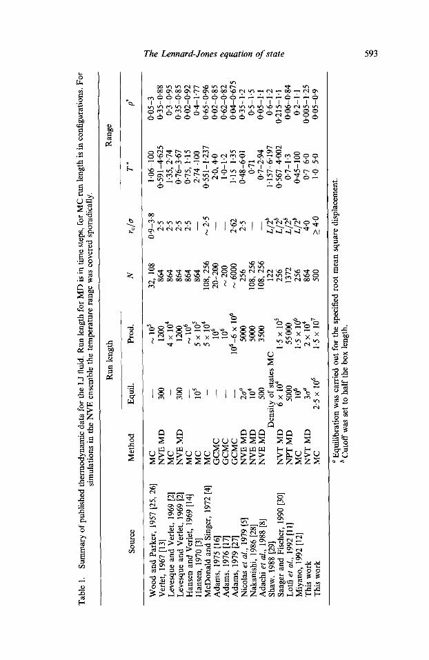
Equations of state for the LJ fluid can be divided roughly into two groups: (1) equations having some theoretical basis (semitheoretical), and (2) purely empirical equations of state. This distinction can become blurred at times because semi- theoretical equations can contain a large number of adjustable parameters, making them much like empirical equations. In this section we review briefly the available equations of state for the LJ fluid. We present a summary of the published equations of state in table 4.

Several equations of state have been published that are based on perturbation

Table 3. Monte Carlo simulation results of this work.

O* T* P* U* rcla

0"5 5.0 4"654(3) -2"365(1) 4"0 0"1 2-0 0"1777(2) -0"667(1) 5"0 0.2 2-0 0.3290(6) -1'306(1) 5"0 0.4 2.0 0'705(1) -2"538(2) 5.0 0"5 2"0 1-069(3) -3"149(2) 5.0 0-6 2"0 1-756(7) -3.746(2) 4.71 0-7 2'0 3.024(7) -4.300(2) 4.47 0-8 2"0 5.28(1) -4-753(3) 4.27 0"9 2.0 9"09(2) -5"030(4) 4-11 0.1 1"2 0.0776(1) -0.840(2) 4.0 0.1 1.15 0-0707(1) -0-869(1) 4.0 0.05 1"0 0.0369(1) -0-478(1) 5.0 0"6 1-0 -0.269(9) -4.228(6) 4-71 0-7 1"0 0"019(10) -4.890(2) 4.47 0"8 1'0 1.03(1) -5.533(1) 4.27 0"8 1"0 1"009(3) -5.5357(6) 4"0 0-9 1"0 3.24(2) -6-062(4) 4' 11

The Lennard-Jones equation of state 601

o

0 o~ c~

o~

0 ~J

Z

%

0

�9 "o "~ ~

~-', ~ o ~ . - ~

~J ~ "~ "~ ~ 0

0 ~ 0 " ~ ' 0

" 0 0 ~

0 0 .~ .~ .

, ~ . . ~ "~ ~ ,.~

~ ' ~ ~ o ~ - -

�9 ~

~ . .

o ~ ~ o ~ o ~ ~, ,~ ~ 0 ~ " ~ ~ ~ ~ - ' L Z ~

~ = ~ 0 ~,.~ ~" ~=~.~ e~.._ ~j ~..~

oo o'~ ~

~ ~ r.,,~ o~

~ e ~ ~ < z ~

o~

0

Io li II

602 J .K . Johnson et al.

expansions about a repulsive reference fluid. Levesque and Verlet [2] were the first to publish an equation of state for the LJ fluid. They presented two semi-theoretical equations based on a A expansion of the attractive part of the potential [36]. The first and second order perturbation terms were fitted to polynomials in density. Hansen [3] fitted a polynomial for the equation of state for a repulsive r -12 potential fluid, and another polynomial for the first order correction term. Ree [7] later modified Hansen's equation by adding a second polynomial for the attractive term that extended the range of applicability. Nezbeda and Aim [9] developed an equation of state based on a first order Weeks-Chandler-Andersen (WCA) perturbation theory [37]. They fitted the attractive term to a polynomial in density and a power-law in temperature. They included pressures, but no internal energies in their regression. Song and Mason [10] developed a WCA-like expansion that depends only on the hard sphere equation of state [38] and three integrals involving the pair potential. Their equation contains no adjustable parameters, but is not as accurate as the other semitheoretical equations.

The strictly empirical equations of state include the following: McDonald and Singer [4], Nicolas et al. [5], S~s and Malijevsk~, [6], Adachi et al. [8] and Miyano [12]. Of these, all but McDonald and Singer used some modified form of the Benedict- Webb-Rubin equation. Because we are using the same form as Nicolas et al. we will discuss their work in more detail. They used a modification of the Benedict-Webb- Rubin equation of state due to Jacobsen and Stewart [39] that contains 32 linear parameters and one nonlinear parameter. This equation has been the most widely used and arguably the most successful of any yet developed for the LJ fluid. The success of the Nicolas equation is probably due to the wide fluid range that it correlates accurately. The MBWR equation has sufficient flexibility to reproduce the properties of the LJ fluid from low to fairly high temperatures and from gas to liquid densities. The equation contains temperature-dependent expressions to account for the first few virial coefficients. While these expressions are entirely empirical, they can give good results if the parameters are regressed properly. This is an advantage over equations of state based on perturbation theories, which are usually inaccurate for low to moderate densities. The disadvantage of an empirical equation of state is that it is not reliable outside the range for which the parameters were determined, and may even give unphysical results. Nicolas et al. regressed the 32 linear parameters based on a data set containing most of the LJ data then published. They also included exact second virial coefficients in the range 0.625 < T* < 20, and 28 low density points generated from the virial series using the first five virial coefficients as calculated by Barker et al. [40]. They constrained their linear optimization to ensure that the equation gave critical constants of To* = 1.35, Pe = 0"35 and Pc = 0.14. The nonlinear parameter in the MBWR equa- tion was optimized by a manual 1-dimensional search.

In passing we note that Lotfi et al. [11] fitted saturation vapour pressures to a Clausius-Clapeyron equation, and saturation densities to a Guggenheim-like expression [41]. While these equations do not constitute a proper equation of state, they do provide accurate correlations for saturation properties. Lotfi et al. also presented a correlation for the saturation chemical potential and the enthalpy of vaporization. The data for these correlations came from their simulations [11].

The Lennard-Jones equation of state 603

Table 5. The a i temperature dependent coefficients for the Helmholtz free energy equation (5). The xj's are the adjustable parameters in the equation of state.

i ai

1 X 1 T* + Xzv/T * + x 3 + x4/T* + x s / T .2 2 x6T, .+.x 7 + x s / T , + x 9 / T 2 3 Xl0 T* +xll +Xl2/T* 4 Xl3 5 X14/T* + X15/T .2 6 Xl6/Z* 7 Xl7/T~2+xls/T .2 8 xI9/T

4. Modified Benedict-Webb-Rubin equation of state

The MBWR equation of state used here is the same as that used by Nicolas et aL [5], and contains 32 linear parameters and one nonlinear parameter. We started by writing the expression for the Helmholtz free energy. We worked in reduced units so A*r =Ar /Ne where Ar is the residual Helmholtz free energy of the fluid (Ar(N , V, T) =- A(N, V, T) - Aid(N , V, T), where Aid is the ideal gas value). A r is given by

8 *i 6

A r = " " * ~ aiPi + E biGi' (5) i=1 i=1

where the coefficients ai and bi are functions of temperature only. These coefficients contain the 32 linear parameters in the MBWR equation. The G i functions contain exponentials of the density and the one nonlinear parameter. The functional forms of the ai, bi, and Gi are given in tables 5, 6 and 7, respectively. From equation (5) we can derive all other thermodynamic properties. The pressure is given by

p* = p*r* + p*2 f OA*~ \ Op* J r*,N' (6)

where P* = Pa3/e includes the ideal gas contribution. Substituting equation (5) into equation (6) gives

Table 6. The bi temperature dependent coefficients for the Helmholtz free energy equation (5). The xj's are the adjustable parameters in the equation of state.

i b i

1 x20/T .2 + x21/T .3, 2 x22/T~ 2 + x23/T*~ 3 x24/T 2 q_ x25/T*~ 4 x26/T .2 q- x27/T* ~ 5 x281T: 2 + x291T* ~ 6 X30/T 2.4_ X31/T*~ "+- X32 / T *4

604 J . K . Johnson et al.

Table 7. The G i density dependent coefficients for the Helmholtz free energy equation (5), where F = exp (-3,p'2), and -y is the nonlinear adjustable parameter. We have chosen

= 3 in this work.

i G i

1 (1 - V2)/(2"y ) 2 -(Fp,Z - 2G1)/(23') 3 - ( F p , ~ - 4G2)/(27) 4 - ( F p 6 _ 6G3)/(27) 5 - ( r p : 8 -- 8G4)/(2"/) 6 - ( F p 1o _ 10G5)/(27)

8 6

P* = p'T* -t- ~ aip *(i+l) @ F ~ bip *(2i+1), ( 7 )

i=1 i=1

where F = exp( -Tp .2 ), 7 is the nonlinear adjustable parameter, and the coefficients ai and b i are the same functions that appear in the Helmholtz free energy expression of equation (5). The residual (configurational) internal energy U* = U r / N e is given by

u; = - r *2 (8) \ OT* Jp, ,u"

Using equation (5) in equation (8) gives

8 C *i 6 v; c,o + : ~-'~diGi, (9)

i i=1 i=1

where the coefficients ci and di are given in tables 8 and 9, and the G i functions are given in table 7. One final property is the Gibbs free energy per atom which, for the pure fluid case, is equal to the chemical potential:

Gr P* G* - Are - #r = Ar + -~- - T*, (10)

where A~ is given by equation (5) and P* is given by equation (7).

Table 8. The ci temperature dependent coefficients for the internal energy equation (8). The xj's are the adjustable parameters in the equation of state.

i ci

1 x2x/T*/2 + x 3 + 2x4/T* + 3 x s / T .2 2 x7 + 2xs /T* + 3x9 /T .2 3 x n + 2x12/T* 4 x13 5 2x14/T* + 3Xls/T .2 6 2x16/T* 7 2x17/T* + 3 x l s / T .2 8 3x19/T .2

The Lennard-Jones equation o f state 605

Table 9. The di temperature dependent coefficients for the internal energy equation (8). The xTs are the adjustable parameters in the equation of state.

i d~

1 3X2o/T .2 + 4x2I/T .3 2 3x22/T .2 + 5x23/T .4 3 3x24/T .2 + 4x25/T .3 4 3x26/T~22 + 5x27/T .4 5 3x28/T,~ + 4x29/T .3 6 3X3o/T ~ + 4x31/T .3 + 5X32/T .4

4.1. Regression o f parameters

We have constrained the equation of state to give a specified critical temperature and density. The MBWR equation is classical and gives a critical exponent of 1/2. Thus, it is incapable of giving a p - T critical region that is sufficiently fiat. Even so, it is important for the equation to give good values of the critical constants. The early estimates for the critical constants [13] were Tc* ----- 1.36 + 0.04 and pc = 0.31 + 0.03. Later, Adams [27] estimated Tc = 1.30 + 0.02 and p~ --0.33 + 0.03. Smit [20, 21] gave estimates based on fitting Gibbs ensemble data to the critical scaling law for density and to the law of rectilinear diameters. His estimates are Te* = 1.316 + 0-006 and Pc = 0.304 + 0.006. Smit used the 3-dimensional critical exponent,/3 = 0.32, in his fitting procedure. Lotfi et al. [11] made estimates of To* = 1.31 and p~ = 0-314 based on their VLE data for the LJ fluid. They did not use the law of rectilinear diameters to determine the critical density; however, their data follow a line of rectilinear diameters extremely well. Applying the law of rectilinear diameters to their data gives p~ = 0.310, slightly lower than the value of 0.314 they report. If we plot the Gibbs ensemble data on the same plot as the data of Lotfi et al. we notice that the low temperature Gibbs ensemble data fall on the same line of rectilinear diameters as the data of Lotfi et al. The Gibbs ensemble data for T* = 1.25 and above deviate from the Lotfi et al. data, but the uncertainties in the Gibbs ensemble data are also large, so that the data agree to within the estimated errors. We have chosen to use pc -- 0.310 and Tc = 1.313 as the best estimates for the critical density and temperature in our equation of state. The critical temperature used is an average of the estimates from the Gibbs ensemble data and from Lotfi's data. The value of p~ depends on To* through the line of rectilinear diameters. However, using the slope from the Lotfi et al. data we find that to three significant figures the value of p~ does not change in going from a critical temperature of 1.310 to 1-313. The constraints for the critical point are

0 / , , Tr162

and

_-o. 0P2,]T to.pc

(12)

We have not specified a value of the critical pressure in the fitting procedure because P~ is not known accurately from simulations. Given the above values of To* and p~,

606 J . K . Johnson et al.

A m

|

0 .20

0 .15

0 .10

0 .05

0 .00

- 0 . 0 5

- 0 . 1 0 0

/ . / . S'

, I

1 1 "#

.~. t . f

i, W lj

i , i . i . t , i i i , �9

2 4 6 8 1'0 1'2 ll4 1'6 18 20

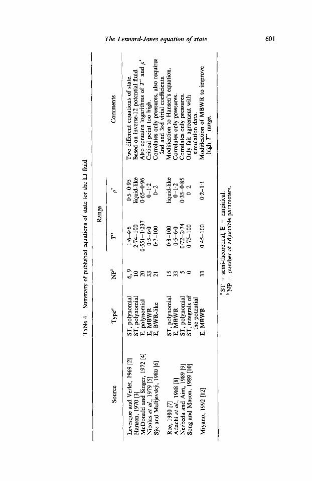
Figure 2. The deviation plot for the reduced second virial coefficient, B* = 3B/(2n~r3), as correlated by the new MBWR parameters (solid line) and the original Nicolas et al. parameters (dot-dashed line). B~*~ is the exact second virial coefficient.

the equa t ion o f s tate wi th the new pa rame te r s gives Pc = 0" 13. The first five pa rame te r s in the M B W R equa t ion (Xl-Xs) de te rmine the second

vir ial coefficient. W e have genera ted exact second vir ial coefficients a t 315 tempera- tures in the range 0.66 < T* < 20 and have used these d a t a to de te rmine the first five pa rame te r s in the M B W R equat ion . W e show the dev ia t ion p lo ts for the second vir ial coefficient f rom our new pa rame te r s and the or ig inal Nico las et al. pa rame te r s in figure 2. The new pa rame te r s corre la te the second vir ial coefficient over a wide t empera tu re range with much h igher accuracy than the Nico las et al. parameters .

Af te r specifying the five pa rame te r s in the second vir ial coefficient cor re la t ion ( x l - x s ) we are left wi th 27 l inear pa rame te r s and one non l inea r p a r a m e t e r to fit. We have used the molecu la r dynamics d a t a l isted in table 2 to regress these pa ramete rs . We weighted the da t a wi th the rec iprocal o f the uncer ta in t ies for bo th the pressures

Table 10. New parameters for the modified Benedict -Webb-Rubin equation of state regressed from the simulation data of this work.

j xj j xj

1 0.862 308 509 750 742 1 17 6.398 607 852 471 505e + 01 2 2.976 218 765 822 098 18 1.603 993 673 294 834e + 01 3 - 8-402 230 t 15 796 038 19 6-805 916 615 864 377e + 01 4 0.105 413 662 920 355 5 20 -2.791 293 578 795 945e + 03 5 -0.856 458 382 817 459 8 21 -6.245 128 304 568 454 6 1.582 759 470 107 601 22 -8.116 836 104 958 410e + 03 7 0.763942 194830 545 3 23 1-488 735 559 561 229e + 01 8 1.753 173 414 312 048 24 - 1.059 346 754 655 084e + 04 9 2-798291772190376e + 03 25 -1-131607632802822e + 02

10 -4 .8394220260857657e- 02 26 -8"867771 540418822e + 03 11 0-996 326 519 772 193 5 27 -3"986 982 844 450 543e + 01 12 -3"698 000 291 272 493e + 01 28 -4"689 270 299 917 261 e + 03 13 2-084 012 299 434 647e + 01 29 2"593 535 277 438 717e + 02 14 8"305 402 124 717 285e + 01 30 -2-694 523 589 434 903e + 03 15 -9"574799715203068e + 02 31 -7.218487631550215e + 02 16 - 1"477 746 229 234 994e + 02 32 1"721 802 063 863 269e + 02

The Lennard-Jones equation o f state 607

8

6

4

2

0

- 2

- 4

- 6

- 8

- 1 0 0

\ \

i I

1 I I I I ] I I I

2 3 4 5

T*

Figure 3. The pairwise-additive reduced third virial coefficient, C* = (3/(2~cr3))2C, from the exact calculations of Barker et al. [40] (o), the new MBWR parameters (solid line), and the Nicolas et al. parameters (dot-dashed line).

and internal energies listed in table 2. For the p* = 0.005 densities with two indepen- dent runs we used the average value of the runs and the sample standard deviation calculated from the two observed points.

We attempted to fit simultaneously the nonlinear parameter 7 and the 27 remain- ing linear parameters by using the Minpack nonlinear optimization package [42]. However, including 7 in the fit made the problem ill-conditioned, and Minpack was not able to find a global minimum. As a result, we regressed the linear parameters at various fixed values of 7 for 1 _< 7 < 7. We observed that the minimum is a very weak function of 7, in agreement with the findings of Nicolas et al. [5]. A shallow minimum from this search routine occurred near 7 = 3.5. However, we have chosen to retain the value 7 = 3 for historical reasons. This does not appreciably affect the accuracy of fit. The final values of the parameters are given in table 10. The fit to the simulation data is very good over most of the T*-p* plane. The average absolute deviations (AAD) are 0.017 in P* and 0"016 in U*. Most of the error for both pressure and internal energy occurs in the region of high temperature and high density, T* > 4.0 and p* > 1.0.

The value of x 2 / N f for this fit is 37.2, where

Np _ x91c)2 X2 = Z (Xistm (13)

;=1 s 7 '

I/tim is the value of either P* or U* from simulation, and Xi ~]~ is the corresponding value from the equation of state. Si is the sample error of the mean as calculated from the simulations, the sum is over the number of points Np, and Nf is the number of degrees of freedom, where Nf = 356 - 27 = 329 in this case.

The reduced third virial coefficient, C* = (3/(2~cr3))2C, is shown in figure 3. While no C* data were directly used in the parameter regression of either Nicolas et al. or this work, we see that the new parameters give qualitatively correct tem- perature dependence of the third virial coefficient. The Nicolas et al. parameters give the wrong qualitative temperature dependence for T* < 2-5. Because this is the temperature region important for VLE, we expect the new parameters to give better saturated vapour densities and energies.

608

0.2

0.0

i - 0 . 2

- 0 . 4

-O.e 0.0

J. K. Johnson et al.

. . �9 , . , - , . ,

A A �9 . _ t i ~ Q . o A

o12 oi~ o16 o15 11o p~

A

A i ,

1.2

I

0.2

0,0

- 0 . 2

- 0 . 4

- 0 . 6 0

V

o o ~ t �9 w w w

O" <>

O I I I i I 1

1 2 3 4 5 8 1"

Figure 4. The deviation plots for pressure, where P~iD denotes the simulation results of this work and P~alc denotes the equation of state calculations with the new MBWR parameters. In the upper figure the triangles are for T* > 5. In the lower figure the diamonds are for #* > 1-1.

I

0.15 r

0.10

0 .05

o.oo tl - 0 . 0 f i

--0.10 0.0

A A A

, ] , 0.2 0 4 0.6

p~

A

A A ~ A

I Jio 8~ - ^

o o o

01.8 1.0 1.2

. t I

0.15 t

0.10 I

--0.05 i -O, lO I-

0 1 2 3 4 5

'I"

O"

v

8

Figure 5. The deviation plots for internal energy, where UI~ID denotes the simulation results of this work and Uc*ale denotes the equation of state calculations with the new MBWR parameters. In the upper figure the triangles are for T* > 5. In the lower figure the diamonds are for p* _> 1.1.

The Lennard-Jones equation o f s tate 609

1 . 4 . u . i - i . i . u , u . i . L

1.3

1.2

1.1

1.0

0.9

0 . 8

0 " 7 7 0 ' 0 . 1 0.2 0.3 0.4 0.5 0.6 0.7 0.8 p*

0.9

Figure 6. Saturation densities from the simulations of Lotfi et al. [11] (solid circles), and predictions from the equation of state using the new MBWR parameters (solid line), and the Nicolas et al. parameters (dot-dashed line). The line of rectilinear diameters is also shown for the simulation results (triangles) and from the equation of state using the new MBWR parameters (solid line).

In figure 4 we show the deviations for the pressure, PlaID- Pcalc, where PMD denotes the MD simulation results, and Pcalc is calculated from the equation of state. The largest errors occur at the highest temperatures and densities. The equa- tion of state does not fit this region particularly well, and one should keep this in mind if properties of the high temperature dense fluid are needed. However, even at the highest absolute error the relative error is only -0-6%, because at this point P* = 85.7. This corresponds to a pressure of about 3-4 GPa for methane. The errors in the internal energy are shown in figure 5. The errors are again largest for the high temperature, high density points. It is apparent from figure 5 that the deviations are not random, but systematic. This indicates that the equation of state is not capable of fitting both the vapour-l iquid region and high temperature region with compar- able accuracy. Although this highlights the shortcomings of the MBWR equation of state, we stress that these errors are still only a few percent at worst.

0 . 1 6 i . u . i . i . u . 0 . i �9

0.14 .i / 0 . 1 2 i /

0.10 ~ / / . / "

& 0.08

0 . 0 6 ..,, "/"

0.04

0.02

0.00 0 1 7 ' 0 ' . 8 ' 0 1 9 ' 1 ' . 0 ' 1'.1 1 1 2 ' 1 ' . 3 ' 1.4

T*

Figure 7. Saturation vapour pressure curve from the data of Lotfi et al. [ll] (points), and predictions from the equation of state using the new MBWR parameters (solid line), and the Nicolas et al. parameters (dot-dashed line).

610 J . K . Johnson et al.

1 . 4 �9 , , i �9 , i . , . , , ,

1.3

1.2

l . l

l.O

0.9

0.8

0.7 0.0 O. 1 0.2 0.3 0.4 0.5 0.6 0.7 0.8 p*

0.9

Figure 8. Saturation densities from the Gibbs ensemble simulations reported in reference [20] (solid circles), and predictions from the equation of state using the new MBWR parameters (solid line), and the Nicolas et al. parameters (dot-dashed line). The line of rectilinear diameters is also shown for the simulation results (triangles) and from the equation of state using the new MBWR parameters (solid line).

The predicted VLE data are compared with data from simulations in figures 6-9. In figures 6 and 7 we see the predictions compared with the VLE data of Lotfi et al. Figure 6 shows the T*-p* projection. We see that the new parameters accurately predict both the vapour and liquid orthobaric densities from about the triple point to close to the critical point. The original Nicolas et al. parameters are quite accurate at low temperatures, but for T ~ > 1 the new parameters are significantly more accu- rate. Figure 7 shows the vapour pressure curve for the LJ fluid. From this figure we see that the new parameters accurately predict the saturated vapour pressures up to the critical point. In figures 8 and 9 we present VLE calculations compared with Gibbs ensemble simulations. The Gibbs ensemble data were taken from the com- pilation in [20]. We see the same results as in figures 6 and 7, except that the Gibbs ensemble data show more scatter, especially at high temperatures. The new

0.16

0.14

0.12

0.i0

0.08

0.08

0.04

0.02

0.00

, , . , , , , ! , , , , �9

/ '

/ /

/ / s

/ - / "

. . . . . . . . i i ' 0.7 0.8 0.9 1.0 1.1 12 13 T*

1.4

Figure 9. Saturation vapour pressure curve from the Gibbs ensemble data reported in reference [20] (points), and predictions from the equation of state using the new MBWR parameters (solid line), and the Nicolas et al. parameters (dot-dashed line).

The Lennard-Jones equation o f state 611

.9 0~ I

0.16

0.12

0.08

0.04

0.00 I

-0.04

-0.08 0.0

4 4

. 4 . t 4

o oo~d o oeO 4

i . i , i , i , i . , . i . l , i

0.1 0.2 0.3 0.4. 0.5 0.6 0.7 0.8 0.9 p~

�9 I

4

o

l] 4 "

�9 i . 4

1 . 0 1 . 1

Figure 10. The difference plot for pressure, where Ps~m are the pressures from references [11, 27, 30], and Pealr is calculated from the MBWR equation of state using the new parameters (circles) and the Nicolas et al. parameters (triangles). None of these data was used in the regression of either the new or the Nicolas et al. parameters. The data cover the temperature range 0.7 < T* < 4.0, with most of the data being at the lower temperatures.

parameters also give fairly good agreement with the older VLE data from the grand canonical simulations of Adams [17, 27]. Although the new equation is more accu- rate than that of Nicolas et al. for VLE calculations, the accuracy of the new equation is somewhat lower for dense fluids at temperatures greater than twice the critical.

We have compared calculations from the new equation with many of the litera- ture data reviewed in section 2.1. In making the comparison, we have excluded data that were outside the fitting range of the new parameters. We find that the newer data [11, 27, 29, 30], which were not included in fitting the Nicolas et al. equation, are in better agreement with the new equation than with that of Nicolas et al. An exception is the data set of Shaw [29], which includes many points in the high temperature, high density range, where the new equation presented here does not perform particularly well. The deviation plots for the pressure data of [11, 27, 30] are shown in figure 10. On the whole, the new parameters give a better representation of the data than the parameters of Nicolas et al.

Schmidt and Wagner [43] developed a MBWR equation for correlating the properties of oxygen and other real fluids. Like the Jacobsen-Stewart MBWR equation used by Nicolas et al., the Schmidt-Wagner (SW) equation contains 32 linear parameters for the residual Helmholtz free energy. However, the terms in the SW equation were selected to give the most efficient representation of experimental data over a limited range. We regressed the parameters in the SW equation from the full LJ data of table 2, but found that the fit was much worse than that of the MBWR equation presented above. We reduced our data set to include only points that were within the reduced pressure range used by Schmidt and Wagner [43] to develop the functional form of their equation (P < 20Pc). However, the X 2 of the fit to the SW equation was still about three times that of the Jacobsen-Stewart MBWR equation fitted to the same range. We conclude that the equation used by Nicolas et al. is better than the SW equation for correlating thermodynamic data for the LJ fluid.

612 J . K . Johnson et al.

5. M B W R for the cut and shifted potential

In table 2 we presented simulation results for both the full LJ fluid and the cut and shifted fluid corresponding to the potential of equation (4). In this section we present an equation of state for the cut and shifted fluid that is based on a simple mean-field correction of the full LJ equation of state presented in section 4.

Powles [44] derived approximate corrections for transforming from the pressure of the full LJ fluid to that of the cut and shifted, and shifted-force fluids. He applied this correction to the Nicolas et al. equation and compared his calculations with a few simulation results for the cut and shifted, and shifted-force potentials. He found good agreement for the cut and shifted fluid. In this section we present a rigorous derivation for the corrections to the Helmholtz free energy, the pressure, and the internal energy.

The change in the Helmholtz free energy due to a change in the potential can be written as a functional derivative [45],

8A ~3-~ = p2g (rl, r2), (14)

where g (rl, r2) is the pair correlation function, r i is the vector defining the position of atom i, and 6q~ is the change in the pair potential. For the change in going from the full LJ potential to the cut and shifted potential

&b(r) = ~bcs(r ) - ~b(r) = { -~b(rc) if r < r c (15) -~b(r) if r > r c'

where ~b(r) is the full LJ potential given by equation (1), ~bcs(r ) is the cut and shifted potential given by equation (4), and r c is the potential cutoff. The change in Helmholtz energy is

V g(r)&k(r)r2 dr (16) A c s - A = 21tNp o

1 . 3 , i . i �9 f �9 i , ~ �9 i i

1.1 I O I - - - - - V - O q

1.o I~" "~ \

0.9 ~ %

0.8

0.7 ~ 0.0' 0'.1' 0'.2' 0'.3' 0:4' 0'.5' 016' 0'.7' 0:8 '

p" 0.9

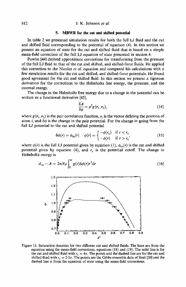
Figure 11. Saturation densities for two different cut and shifted fluids. The lines are from the equation using the mean-field corrections, equations (18) and (19). The solid line is for the cut and shifted fluid with r c = 4c~. The points and the dashed line are for the cut and shifted fluid with r e = 2"5o'. The points are the Gibbs ensemble data of Smit [20] and the dashed line is from the equation of state using the mean-field corrections.

The Lennard-Jones equation of state 613

0 .09

0.08

0.07

0.06

0 .05

0 .04

0 .03

0.02

0.01

0.00

i r

017 ' 018 ' 01~ ' 110 T'

1.1

Figure 12. The vapour pressure curve for the cut and shifted fluid with rc = 2.5tr. The points are the Gibbs ensemble simulations of Smit [20], and the line is calculated from the equation using the mean-field corrections to the cut and shifted fluid.

= ,27rNp[(9(rc)Ii~g(r)r2dr+ Jr~g(r)q~(r)r2dr], (17)

where equat ion (15) has been used for 6~b(r). Next we introduce two approximations. We first assume that g(r) = 1 for r > r c. Next we notice that 2np~~ in equat ion (17) is just the number o f pairs o f a toms within the cutoff o f a central atom. We approximate this by the average number o f pairs o f a toms in the volume o f a sphere o f radius r e. This leads directly to

7~ - ~ 7~ " (18)

We can calculate the correct ion to the internal energy by substituting equat ion (18) into equat ion (8); it is exactly equal to the right hand side o f equat ion (18).

1.20

1.15

1.10

1.05

1.00 0.0

z.9,, ~ \

0.1 0 .2 0.3 0 .4 0.5 0 .6 0.7 p*

Figure 13. Saturated densities in the critical region from the mean-field approach, equations (18) and (19), for the cut and shifted fluid at several different values of the cutoff, r c.

614 J . K . Johnson et al.

The pressure correction is calculated from equations (18) and (6) and is given by

pes-p*-32~p*2[(tr) 9 3 ( t r ) 3] - ~ ~ . (19)

These two approximations are made in the spirit of mean-field theory, and therefore we refer to equations (18) and (19) as the mean-field corrections for the cut and shifted fluid. Note that equation (19) is the same as equation (2) for the tail correction to the pressure except for the sign. This is because the shift in the potential does not affect the pressure. The correction to the energy is not the same as the tail, equation (3), because the energy depends on contri- butions form both the potential shift and the cutoff. We have applied these corrections to the full MBWR equation of state and compared predictions from this new equation of state with the cut and shifted simulation data of table 2. We find that calculations from the mean-field equations for the cut and shifted fluid are about as accurate as the fit to the full LJ data. The AAD for P* is 0"017 and for U* the AAD is 0-016, and the value of x2/Nr is 34.4, for Nf = 356, which indicates that the mean-field approximations are very accurate for this cutoff. The critical properties predicted from equation (19) are Te* = 1.246, p~ = 0.308 and Pc = 0-118, for r c -- 4or.

This mean-field approach is not limited to a cutoff of 4a, of course. The same equations may be applied to any cutoff. However, the accuracy of both approximations will deteriorate as rc becomes smaller. In figure 11 we present the T*-p* projection of the vapour-liquid phase diagram for the cut and shifted fluid for two different values of r e . The solid line was calculated from the mean-field approach with r c = 4a, while the dashed line is for r e --2.5tr. The points are the Gibbs ensemble results of Smit [20] with re = 2-5tr. We see that the mean-field approach gives very good agreement with the Gibbs ensemble results for T* < 1, but the equation of state predicts a lower critical temperature and exhibits an unphysical hump in the phase diagram near the critical point, as was noted by Smit [20, 21]. Figure 12 shows the vapour pressure plot for the cut and shifted fluid with r e = 2-5cr from the equation of state and from simulations. The mean-field approach predicts the saturation pressures to within the accuracy of the simulations, except near the critical point. The unphysical hump in the phase dome may be related to a problem noted by Reddy and O'Shea [46], who regressed parameters for the MBWR equation of state from data for the 2-dimensional LJ fluid. They did not fix the values of the critical temperature and density in fitting the parameters, and found that the resulting equation had three solutions for the critical conditions (11) and (12). We have searched for the critical points of the MBWR equation using a nonlinear root finding routine to solve equations (11) and (12) by starting from various initial guesses. For re = 2"5tr the equation predicts three critical points, the (T*,p*) coordinates of which are (0.7248, 0.3432), (1-0017, 0-329), and (1.0399, 0.2215). These last two critical points are very close, and are perhaps responsible for the unphysical region in the phase diagram. We have tested the limit of applic- ability of the mean-field equation by examining the saturation densities in the critical region for various values of re (figure 13). We find that the unphysical hump begins to appear around r e = 2-9tr, and therefore conclude that the mean-field equations for the cut and shifted fluid should give reasonable results for r e > 3a.

The Lennard-Jones equation of state 615

0.201 �9 , - , �9 , . , . . . . . . �9 , . , .

t

O. 16 t ~ _ ~ , ~ , / = 1.0 i r. ~0.75 . t ,

000" ' , :,-':l 0.0 0.1 0.2 0.3 0.4 0.5 0.6 0.7 0.8 0.9 1.0

Xt, Y~

Figure 14. Vapour-liquid equilibrium calculations for LJ mixtures from the Gibbs ensemble simulations of reference [49] (points) and from the equation of state with new parameters (lines). The LJ parameters are e22/~11 = 0.5 and ~r22/~rll = 1. The Lorentz- Berthelot combining rules are used for the cross-interactions.

6. Extension to mixtures

The MBWR equation was developed for pure fluids. Any attempt to apply this equation to mixtures must include some approximate theory such as the conformal solution theory or corresponding states [47]. The most successful conformal solution theory is the van der Waals one-fluid theory (vdWl). The vdWt theory is capable of predicting accurately the behaviour of fluid mixtures if the difference in size or energy parameters is not too large. Shing and Gubbins [48] found that vdWl gives good results for Henry's law constants when the difference in the LJ size parameter is not more than about 10%. Harismiadis et al. [49] found fairly good results using vdW1 for phase equilibrium calculations of binary LJ mixtures, even when both the size and energy parameters differed by a factor of 2. Their results suggest that phase

1.2

1.0

0.8

0.6

0.4

0.2

0.0 . . . . . . . . . . . . . . . . . . . 0.0 0.1 0.2 0.3 0.4 0.5 0.8 0.7 0.8 0.9 1.0

Xt, Yt

Figure 15. Vapour-liquid equilibrium calculations for LJ mixtures from the Gibbs ensemble simulations of reference [49] (points) and from the equation of state with new parameters (line). The LJ parameters are e22/c11 = 0.5 and ~22/all = 0-5. The Lorentz- Berthelot combining rules are used for the cross-interactions.

616 J . K . Johnson et al.

equilibrium calculations are less sensitive to mixing rules than excess properties or infinite dilution chemical potentials.

The vdWl mixing rules for the LJ fluid are

and

3

= Z Z i j

(20)

where (Oox ] The last term in equation (22) simplifies after some algebra to

( OA*'~ = (~.2 T* [ ['Ocr3x'~ ] (A* - Ur*) (Oex'~ (25)

Note that equations (22-25) contain both reduced (p*) and unreduced (p) densities. We have performed phase equilibrium calculations for three binary LJ mixtures

and compared the results with Gibbs ensemble simulation data from reference [49]. In figure 14 we present the data for a mixture with the LJ parameters e22 = 0"5ell and cr22 =t r l l . The Lorentz-Berthelot combining rules were used for the cross- parameters. The agreement between simulation and the equation of state is generally quite good. The predicted critical points are somewhat too high in pressure, and the liquid phase mole fractions are also high. The P, X, Y diagram for the system with e22 --- 0"5eu and ~r22 = 0"5~rl1 is shown in figure 15. Even for this highly asymmetric mixture the vdW1 mixing rules give surprisingly good results for the pressure and mole fractions.

(24)

1 3 ex = --~ Z Z XiXjeij~rij, (21) x i j

where the subscript x denotes the mixture property and X,. is the mole fraction of component i in the mixture. The cross-interaction parameters e/j and a~j are often chosen by some kind of combining rules, e.g., Lorentz-Berthelot.

The MBWR equation of state used in this work gives the Helmholtz free energy as a function of p* and T*. For mixtures we use the same functional form, but the inde- pendent variables become composition-dependent through p* = pcr3x and T* = k T/ex. The reduced thermodynamic properties are also explicitly composition-dependent: A*r Ar/Nex, P * = 3 * = P~rx/e x, and Ur = U/Ncx. The chemical potential for com- ponent i in the mixture can be calculated from

(OAr~ (O(NA*rex)~ I'Zr'i = t-'~iiJ T,V, Nj#,= ~ ONi ] r,v,~,,,

.. [Oex'~ +pex(OA*~ (22) = A*, x -I- ArPt~Pi ) T,p,., \ OPi J T,.,@i

The partial derivatives require derivatives of the mixing rules.

op,) t.op, ) p

The Lennard-Jones equation o f state 617

7. Conclusion

We have presented accurate new MD simulation results for the LJ fluid at 175 different state points over a wide range of temperature and density, together with a few MC simulation data.

Parameters for the MBWR equation of state for the LJ fluid have been regressed for the temperature range 0-7 < T * < 6 and covering the entire fluid range of densities. The equation is especially accurate for vapour-liquid equilibrium calcula- tions. Agreement for saturated densities and vapour pressures is seen with Gibbs ensemble, N P T + particle insertion, and grand canonical Monte Carlo simulations. Because we have no more parameters at our disposal than did Nicolas et al., this improved accuracy for phase equilibrium calculations has come at the expense of some loss of accuracy for liquid states at sub-triple point temperatures and at high temperatures (T* > 4) and high densities (p* > 1-0).

We have presented an equation of state for the cut and shifted fluid that is based on a mean-field correction to the equation of state for the full LJ fluid. This method is applicable for any cutoff; however, the accuracy decreases as the cutoff decreases. For values of r c < 3a~ the equation fails to give physically meaningful results in the critical region.

We have performed calculations for various LJ binary mixtures with the van der Waals one-fluid theory, using the MBWR equation for the reference fluid. These calculated values have been compared with Gibbs ensemble simulation data. Predic- tions from the equation of state are in quite good agreement with the simulation results for the pressures and compositions.

We thank Drs. F. van Swol, S. M. Thompson, and B. Smit for helpful discus- sions. This work was supported under contract number 5091-260-2255 from the Gas Research Institute, and in part by the National Science Foundation (grant number CTS-9122460).

References

[1] MAITLAND, G. C., RIGBY, M., SMITH, E. B., and WAKEHAM, W. A., 1981, Intermolecular Forces (Clarendon Press).

[2] LEVESQUE, D., and VERLET, L., i 969, Phys. Rev., 182, 307. [3] HANSEN, J.-P., 1970, Phys. Rev. A, 2, 221. [4] McDONALD, I. R., and SINGER, K., 1972, Molec. Phys., 23, 29. [5] NICOLAS, J. J., GuaBrNS, K. E., S3"REEYr, W. B. and TILDESLEY, D. J., 1979, Molec. Phys.,

37, 1429. [6] Sqs, J., and MALIJEVSK~', A., 1980, Collec. Czech. Chem. Commun., 45, 977. [7] REE, F. H., 1980, J. chem. Phys., 73, 5401. [8] ADACHI, Y., FIJIHARA, I., TAKAMIYA, M., and NAKANISHI, K., 1988, Fluid Phase Equilibria,

39, 1. [9] NEZBEDA, I., and AIM, K., 1989, Fluid Phase Equilibria, 52, 39.

[10] SONG, Y., MASON, E. A., 1989, J. chem. Phys., 91, 7840. [11] LOTFI, A., VRABEC, J. and FISCHER, J., 1992, Molec. Phys., 76, 1319. [12] MIYANO, Y., 1992, Fluid Phase Equilibria, in press. [13] VERLET, L., 1967, Phys. Rev., 159, 98. [14] HANSEN, J.-P., and VERLET, L., 1969, Phys. Rev., 184, 151. [15] VERLET, L., and WEIS, J.-J., 1972, Phys. Rev. A, 5, 939. [16] ADAMS, D. J., 1975, Molec. Phys., 29, 307. [17] ADAMS, D. J., 1976, Molec. Phys., 32, 647. [18] PANAGIOTOPOULOS, A. Z., 1987, Molec. Phys., 61, 813.

618 J . K . Johnson et al.

[19] PANAGIOTOPOULOS, A. Z., QUIRKE, N., STAPLETON, M., and TILDESLEY, D. J., 1988, Molec. Phys., 63, 527.

[20] SMIT, B., 1990, Ph.D. Dissertation, University of Utrecht, The Netherlands. [21] SMIT, B., 1992, J. chem. Phys., 96, 8639. [22] SMIT, B., DE SMEDT, PH., and FRENKEL, D., 1989, Molec. Phys., 68, 931. [23] SMIT, B., and FRENKEL, O., 1989, Molec. Phys., 68, 951. [24] ALLEN, M. P., and TILDESLEY, D. J., 1987, Computer Simulation of Liquids (Clarendon

Press). [25] WOOD, W. W., and PARKER, F. R., 1957, J. chem. Phys., 27, 720. [26] WOOD, W. W., 1968, Physics of Simple Liquids, edited by H. N. V. TEMPERLEY,

J. S. ROWLINSON and G. S. RUSHBROOKE (North-Holland). [27] ADAMS, D. J., 1979, Molec. Phys., 37, 211. [28] NAKANISHI, K., 1986, Physica, 139 & 140B, 148. [29] SHAW, M. S., 1988, J. chem. Phys.,.89, 2312. [30] SAAGER, B., and FISCHER, J., 1990, Fluid Phase Equilibria, 57, 35. [31] VOGELSANG, R., and HOHEISEL, C., 1985, Molec. Phys., 55, 1339. [32] THOMPSON, S. M., 1992, unpublished data. [33] BisHop, M., and FraNKS, S., 1987, J. chem. Phys., 87, 3675. [34] SWOPE, W. C., ANDERSEN, H. C., BERENS, P. H., and WILSON, K. R., 1982, J. chem. Phys.,

76, 637. [35] CHOKAPPA, D. K., and CLANCV, P., 1988, Molec. Phys., 65, 97. [36] BARKER, J. A., and HENDERSON, D., 1967, J. chem. Phys., 47, 2856, 4714. [37] WEEKS, J. D., CHANDLER, D., and ANDERSEN, H. C., 1971, J. chem. Phys., 54, 5237. [38] CARNAHAN, N. F., and STARLING, K. E., 1969, J. chem. Phys., 51, 635. [39] JACOBSEN, R. T., 1972, Ph.D. Thesis, Washington State University; JACOBSEN, R. T.,

STEWART, R. B., 1973, J. Phys. Chem. Ref. Data, 2, 757. [40] BARKER, J. A., LEONARD, P. J., and POMPE, A., 1966, J. chem. Phys., 44, 4206. [41] GUGGENHEIM, E. A., 1945, J. chem. Phys., 13, 253. [42] MORI~, J. J., GARBOW, B. S., and HILLSTROM, K. E., 1980, User Guide for Minpack-1,

Argonne National Labs Report ANL-80-74. [43] SCHMIDT, R., and WAGNER, W., 1985, Fluid Phase Equilibria, 19, 175. [44] POWLES, J. G., 1984, Physica A, 126, 289. [45] RICE, S. A., and GRAY, P., 1964, Supplement in FISHER, I. Z., Statistical Theory of

Liquids, (University of Chicago Press). [46] REDDY, M. R., and O'SHEA, S. F., 1986, Can. J. Phys., 64, 677. [47] McDONALD, I. R., 1973, Statistical Mechanics, Vol. l, edited by K. Singer (Specialist

Periodical Report, The Chemical Society). [48] SHING, K. S., and GUBBINS, K. E., 1982, Molec. Phys., 46, 1109; 1983, 49, 1121. [49] HARISMIADIS, V. I., KOUTRAS, N. K., TASSIOS, D. P., and PANAGIOTOPOULOS, A. Z., 1991,

Fluid Phase Equilibria, 65, 1.