May 1st, 2018 Geog. 578 Final Paper

A GIS Analysis of Emergency Medical Services Response in Denver, Colorado

David Waro, Casey Kalman, Albert Dudek

1. Introduction

Emergency medical services (EMS) exist to ensure a better quality of life. EMS

has improved in accessibility and responsiveness since its conception and is

responsible for saving countless lives. The increased effectiveness of EMS has

provided immediate medical assistance to those who are in need of help. Without EMS,

the fatality rate of emergencies, including heart attacks, stroke and car accidents, would

be undoubtedly be higher than the observed rate. We seek to explore the geographic

variation in accessibility to EMS within the Denver area in order to reveal disparities that

may exist as a result of natural, human-made, or socioeconomic barriers. To complete

this analysis, we will execute a network analysis to calculate response time patterns and

identify underserved areas.

2. Background

The standardized system of emergency medical services that we utilize today,

including pre-hospital care and medication, was formalized in the 1960s. In 1966,

President Lyndon B. Johnson was presented with a white paper detailing the large

number of lives being lost every year to accidental deaths. In 1965 alone, the number of

lives lost to accidental death was greater than the number of American lives lost in the

Korean War (Edgerly 2013). This white paper lead to the standardization of training for

ambulance staff as well as firefighters, police officers, and volunteer rescue squads.

Since the 1970s, the effectiveness of EMS has continuously improved with

increased research interests and political efforts. The indicators used to measure

effectiveness can be divided into three categories: structure, process, and outcomes

(Brodsky 1983). Structure most often refers to the number and location of EMS stations

as well as the number of ambulatory vehicles. Measuring effectiveness based on

outcomes refers to health outcomes of the patients serviced, which include survival rate

and any resulting disabilities (Brodsky 1983). This analysis will focus on the process

category, which includes, among other factors, response time.

The National Fire Protection Association's standard response time for a life-

threatening emergency is eight minutes and forty-nine seconds. In the case of cardiac

arrest, it is vital for a patient to receive medical attention within four minutes (Zaffar

2016). The ability of an ambulance to quickly arrive at a medical emergency site and

then continue on to the hospital is key to improving outcomes and saving lives.

Regarding certain types of medical emergencies such as severe asthma attacks,

it has been shown that there is a significant difference in service utilization for different

demographic groups. One study in Houston revealed that census tracts with higher

rates of EMS utilization for asthma attacks had higher percentages of individuals who

were low-income, African American, female, and had larger counts of individuals without

a high school diploma. The study also showed that certain racial and gender groups are

more likely to seek EMS services after regular office hours (when doctor’s offices are

likely closed) (Raun 2015).

Given the variation of service utilization based on demographics as well as the

importance of response time, this analysis will aim to identify census tracts with high

travel times. These areas will then be examined further to reveal if there is a correlation

between high travel times and certain demographic groups.

3. Conceptualization

While developing the conceptualization diagram, two key concepts were first

defined: emergency medical services and demographics. Emergency medical services

include four variables: incident point, starting point, end point, and EMS catchment. The

incident point is the location of the medical emergency. To determine incident points we

will use census tract centroids. The starting point is the location of the nearest EMS

station to the specific incident point. The end point is the nearest hospital from the

incident point. The EMS catchment will be created by using Voronoi polygons. The EMS

catchment area is useful in visualizing an area to distinguish which specific EMS station

is closest to the incident point. Demographics includes three variables: age, income,

and race. Income will be split into rich and poor, meaning that an income that is greater

than or equal to the median income is considered rich. Age will be similarly compared

by using the median age as the threshold for young and old. Race will be treated as

binary, with white and minority classifications. This will be defined by one- hundred

percent less the percentage of white residents for a given census tract.

-- Conceptualization Diagram - Denver EMS

4. Methods

When analyzing emergency medical services, it is important to touch on how

each step of the process is being considered in order to highlight assumptions being

made as well as to eliminate ambiguity. Our analysis required us to make assumptions

that may not have reflected exact situations that would be occurring. For example, we

made the assumption that all drive times are calculated with light traffic, i.e., traffic

concerns will not be playing a role in our analysis. With additional time and pending how

our original analysis process goes, we may be extending our project to better capture

the variability in the traffic situations that occur while completing our drive times study.

Our methods consist of geocoding, space partitioning, a road network analysis, and

lastly finding a correlation between our resulting drive times layer and demographic

information.

A. Geocoding

The first step in our analysis was to convert our emergency medical services and

hospital layers to usable formats to be used in a geographic information system (GIS).

In order to do this, the address field was geocoded to receive latitude and longitude

coordinates. We did this through a python script which made use of the geocoder,

pandas, os, time and geopy python packages. The script first takes our list of addresses

and searches Bing’s location services through its application programming interface

(API) to return coordinate positions. Any address not found with Bing’s services are then

run through Google’s location services. If any addresses are still left unfound, they will

be manually searched, although we expect this number of locations to be nominal in

size.

B. Catchment Areas - Voronoi Polygons

The next step was to create catchment areas for our EMS stations. These

catchment areas were formed using Voronoi polygons. Voronoi polygons result from a

points data layer. The main idea is that the two-dimensional plane is partitioned around

n points given as input (our EMS stations), and any point within each of these convex

polygons is understood to be closest to the generating point (again, our EMS stations)

(Weisstein 2018). Therefore, any census tract centroids within a given polygon will take

the generating point EMS station as the closest emergency medical responder and this

will be the station with which we start our drive time calculation.

C. Drive Time Analysis

The bulk of the project’s analysis was derived using drive times. We utilized

Google Map’s Python googlemaps package to calculate drive times. In order to use this

package, we first needed to reformat the data. This required nominal changes to the

data such as making sure all of the coordinates for each of the census tract centroids,

EMS stations, and hospitals were respectively combined (latitude and longitude) as one

string. When the data was prepared, we first calculated drive times for each centroid

from the closest EMS station. We already knew the associated closest EMS station to

each centroid from creating the voronoi polygons layer previously. The second step of

the process involved finding the closest hospital to each centroid. We differenced

coordinates of centroids and hospitals to find the minimum distance to a hospital and

then associated that hospital with the respective centroid point. We then repeated the

same process as before with the EMS stations to calculate drive times, only the centroid

was now the starting point and the hospital location was now the end point. There was

one centroid location that gave the script issues, the Rocky Mountain Arsenal National

Wildlife Refuge tract. To deal with this, the centroid’s coordinates were changed to the

entrance road parking area of the refuge. To create the total drive times field, we then

simply summed the two drive times from the EMS station to the census tract centroid,

and then from the centroid to the hospital.

D. Demographic Correlation

Our next step was to connect the EMS drive times analysis to the census

gathered demographic information. We will be looking to reveal any insights regarding

emergency response accessibility to different groups of people. Our characteristics of

focus: income, age, and race. We will use the respective median values for income and

age given their associated census tracts. Race will be treated as a binary classification

between white and non-white. Percent non-white for the census tract will be calculated

as one-hundred percent less the percentage of white residents. At this stage, we do not

have any bias involved in our search for correlations between drive times and

accessibility to different demographics. This is to say, we are not attempting to rebuke

or advocate for any noted claims, this project is designed to simply explore the data to

reveal if there are patterns of underserved communities within the Denver area.

E. Regression

To further explore the relationship between the total drive time and the

demographics of different census tracts, a linear model was fit to the data. Total drive

time from EMS station to census tract centroid and then to the nearest hospital was

treated as the dependent variable. Percent non-white, median age, and median income

were used as the independent variables.

Before fitting a linear model, summary statistics as well as histograms of each

variable were created in order to understand the nature of the raw data and to

determine whether the data fulfilled the necessary assumptions for fitting a linear model.

The entirety of this statistical exploration and regression analysis was carried out using

R Studio. The R code that was utilized can be found in Appendix B.

The initial summary statistics showed that the standard deviation and variance of

each variable varied by more than two orders of magnitude. This is due to the fact that

the median income data was on a much larger scale than the race and age data.

Because of the difference in scale, it was determined that the data would need to be

standardized in order to fit a linear model.

Histograms for each variable were also created in order to establish the normal

distribution of the data. The histograms reveal that the data for percent non-white,

median income, and total drive time all show a rightward skew. Because of this, it was

determined that some kind of transformation would be necessary for a linear model.

Next, a matrix of scatterplots was created in order to determine if collinearity could arise

as an issue. The relationship between median age and percent non-white showed

strong potential for collinearity. To explore this relationship further, correlation and

covariance matrices were produced to check for problematic collinearity.

The covariance matrix below shows that there are values close to 0 -- which

would indicate perfect independence; however, none of the variables show perfect

linear independence. The correlation matrix shows that none of the variable pairs have

a correlation value close to the absolute value of one, which would indicate a high

correlation. The highest correlation was between the percent non-white and median

age. The relationship between percent non-white and drive time showed a moderate

amount of correlation. A variance inflation factor was calculated, which confirmed we did

not have to remove any of the variables due to collinearity; however, after this

exploration of the data, it was determined that standardization would be needed. The

scale function in r would be used to achieve this.

Finally, a linear model was fit to the unstandardized and untransformed data in

order to check for heteroscedasticity. After a linear model was fit, the following summary

plots show that there is a slight megaphone shape to the residual plot as well as some

potential outliers. The outlier test function was used to confirm the outliers that should

be removed from the model and those observations were removed from the data. The

shape of the residual plot also confirmed that the data should be transformed.

Lastly, we used the box cox method to determine the most appropriate

transformation. After using the boxcox function in r, it was determined that a power of .5

or square root transformation would be most appropriate. A new model was created

with the scaled data that included the new transformation. Finally, a backwards step

function was applied in order to decide which variables should be included in the model.

The final model:

sqrt(drive time) = 5.88900 - 0.00013(Median Income) - 2.83479 (Percent Non-White)

5. Results

A. Age

B. Income

C. Race

While analyzing the connection between percent non-white and drive time we

found that there was a slight inverse relationship between the two. There was a

coefficient value of -0.15 for the respective constant fitting the drive time and percent

non-white relationship. This was the largest value found between drive time and any of

the three operationalized demographic variables. Using a bivariate map (see figure 4

below) of drive times and percent non-white we can begin to find spatially where this

relationship might be found. The center of the city bolsters the census tracts with the

highest percent non-white demographic. We see particularly low drive times for most of

the tracts in the downtown (near center) area both connected to high and low percent

non-white tracts.This is mainly because the hospital and ems locations are concentrated

in the downtown area. As we move out from the center of the city, we see the drive

times increase as we would expect, and we also see the percentage of white residents

within census tracts increase. This phenomena best captures the slight inverse

relationship between non-white residents and drive times. With the highest values of

non-white residents centered in the Denver area, they are prone to have lower drive

times associated while the majority of the tracts surrounding the city center are mainly

white.

6. Discussion

In order to start our analysis, we had to make certain assumptions. Our study

area was essentially the Denver area encompassed by Highway 470. This was an

arbitrary way to define our study area, and we acknowledge that there could be

hospitals or EMS stations just outside the boundary that could lead to different results.

Secondly, we calculated drive times using light traffic conditions. This is not always

going to be the case, and EMS are allowed to exceed speed limits, so drive times will

not be exactly representative of raw values. From the incident point, we decided that the

EMS will always drive to the closest hospital, which is not always the case. Lastly, all of

our operationalized variables were defined in a manner we saw best fit, but this does

not necessarily mean that this is the only way to study accessibility to emergency

medical services.

We ended this analysis with a new original data layer. This layer contains EMS

locations around the Denver area with the following associated information (given they

are serving census tract centroid locations): locations (census tract centroid locations)

that they will serve, the distance there, the drive time to get there, the closest hospital,

its distance, and the drive time to get there. Having information like this on hand can

allow EMS to better prepare for arriving at an incident because they can connect the

type of accident and what state the situation will be in given the amount of time it will

take them to drive there. This information would also be valuable to governing bodies

looking to expand EMS and hospital locations in the future.

7. Conclusion

The focus of this GIS analysis was to explore the geographic variation in

accessibility to EMS within the Denver area and to reveal if there were any

shortcomings regarding accessibility across different demographics. Because it was an

exploratory analysis, we were not specifically biased towards finding a particular result.

After running a regression function for drive times associated with each demographic,

we found low levels of significance. The only usable coefficient was is that of drive times

slightly inversely associated with the non-percent white field. With this, we also found

that census tracts with higher percentages of non-white residents tended to be located

near the center of the city, which is also where the majority of the hospitals are

clustered. Through different Python and R scripts as well as using a GIS system, we

were able to fully implement this analysis. With the exception of the creation of the map

visuals, which required unique cartographic attention, this project contained steps and

scripts that should allow the work to be reproducible for new studies in different cities

given new data sets. We have been able to reveal trends about the city and how they

are connected to drive times regarding medical attention. However, at this stage we do

not have any recommendations to the respective EMS governing bodies of Denver for

new locations or adjustments to increase accessibility to these services.

Works Cited

Brodsky, Harold, and A.shalom Hakkert. “Highway Fatal Accidents and Accessibility of

Emergency Medical Services.” Social Science & Medicine, vol. 17, no. 11, 1983, pp.

731–740., doi:10.1016/0277-9536(83)90261-7.

Eric, Weisstein. 2018 “Voronoi Diagram.” MathWorld--A Wolfram Web Resource.

http://mathworld.wolfram.com/VoronoiDiagram.html.

Esri. 2018 “Algorithms Used by the ArcGIS Network Analyst Extension.” Arcmap.

http://desktop.arcgis.com/en/arcmap/10.5/extensions/network-analyst/algorithms-

used-by-network-analyst.htm#GUID-D50336EC-7FBA-43FA-AD31-4272AB544393.

Raun, L.h., et al. “Factors Affecting Ambulance Utilization for Asthma Attack Treatment:

Understanding Where to Target Interventions.” Public Health, vol. 129, no. 5, 2015, pp.

501–508., doi:10.1016/j.puhe.2015.02.009.

Zaffar, Muhammad Adeel, et al. “Coverage, Survivability or Response Time: A

Comparative Study of Performance Statistics Used in Ambulance Location Models via

Simulationâ “Optimization.” Operations Research for Health Care, vol. 11, 2016, pp.

1–12., doi:10.1016/j.orhc.2016.08.001.

APPENDIX

A. Sample of drive times script

ems_cent_drive = [] cent_hosp_drive = [] total_drive_time = [] for row in data: # centroid coords row[12] # hospital coords row[13] # ems station coords row[14] now = datetime.now() # generates results ems_cent_result = gmaps.directions(row[14], row[12], mode="driving", avoid="ferries", departure_time=now ) cent_hospital_result = gmaps.directions(row[12], row[13], mode="driving", avoid="ferries", departure_time=now ) # append the results' drive times to lists try: ems_cent_drive.append(ems_cent_result[0]['legs'][0]['duration']['text']) cent_hosp_drive.append(cent_hospital_result[0]['legs'][0]['duration']['text']) # convert drive times to usable numbers if len(ems_cent_result[0]['legs'][0]['duration']['text']) == 5: ems_drive_time = float(ems_cent_result[0]['legs'][0]['duration']['text'][:-4]) else: ems_drive_time = float(ems_cent_result[0]['legs'][0]['duration']['text'][:-5]) if len(cent_hospital_result[0]['legs'][0]['duration']['text']) == 5: hosp_drive_time = float(cent_hospital_result[0]['legs'][0]['duration']['text'][:-4]) else: hosp_drive_time = float(cent_hospital_result[0]['legs'][0]['duration']['text'][:-5]) # calculate total drive time

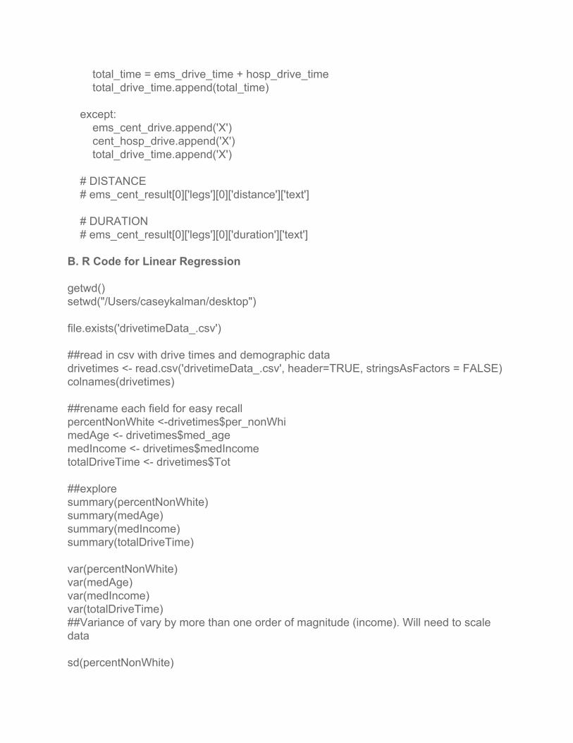
total_time = ems_drive_time + hosp_drive_time total_drive_time.append(total_time) except: ems_cent_drive.append('X') cent_hosp_drive.append('X') total_drive_time.append('X') # DISTANCE # ems_cent_result[0]['legs'][0]['distance']['text'] # DURATION # ems_cent_result[0]['legs'][0]['duration']['text'] B. R Code for Linear Regression getwd() setwd("/Users/caseykalman/desktop") file.exists('drivetimeData_.csv') ##read in csv with drive times and demographic data drivetimes <- read.csv('drivetimeData_.csv', header=TRUE, stringsAsFactors = FALSE) colnames(drivetimes) ##rename each field for easy recall percentNonWhite <-drivetimes$per_nonWhi medAge <- drivetimes$med_age medIncome <- drivetimes$medIncome totalDriveTime <- drivetimes$Tot ##explore summary(percentNonWhite) summary(medAge) summary(medIncome) summary(totalDriveTime) var(percentNonWhite) var(medAge) var(medIncome) var(totalDriveTime) ##Variance of vary by more than one order of magnitude (income). Will need to scale data sd(percentNonWhite)

sd(medAge) sd(medIncome) sd(totalDriveTime) par(mfrow=c(2,2)) hist(percentNonWhite, main="percent nonWhite", breaks=20) hist(medAge, main="Median Age", breaks=20) hist(medIncome, main="Median Income", breaks=20) hist(totalDriveTime, main="total drive time", breaks=20) ##All data are skewed except the median age. Will need to transform ##Check potential for colinearity pairs(~totalDriveTime+percentNonWhite+medIncome+medAge) pairs(drivetimes) ##potential collinearity between percentNonWhite and median age. Nothing else looks super strong ##Calculate correlation matrix cor(drivetimes) ##Calculate covariance matrix cov(drivetimes) ##fit a linear model to "raw" data. not scaled. not transformed model1 <- lm(totalDriveTime~percentNonWhite+medIncome+medAge) model1 ##plot the model par(mfrow=c(2,2)) plot(model1) ##nonconstant variance, potentially non normal distribution, one potential outlier ##outlier test library(car) outlierTest(model1) ##p value is less than .05, potentially significant ##remove obsrvation 427 drivetimes2 <- drivetimes[-427,] ##standarize the dataset drivetimes2 <-scale(drivetimes2) drivetimes2 <-as.data.frame(drivetimes2) ##rename variables within new table without outlier

totalDriveTime2 <- drivetimes2$Tot percentNonWhite2 <- drivetimes2$per_nonWhi medIncome2 <- drivetimes2$medIncome medAge2 <- drivetimes2$med_age ##fit a new model model2 <-lm(totalDriveTime2~percentNonWhite2+medIncome2+medAge2) ##fit new linear model without the outlier and create summary plots par(mfrow=c(2,2)) plot(model2, main="model 2") outlierTest(model2) ##Potential outlier: Observation 526. Bonferonni p value greater than .05. No need to delete the observation ##test for variance inflation factor to determine if collinearity is an issue vif(model2) ##Still seeing a cone shape on the residual v. fitted graph. Will use boxcox method to transform library(MASS) model.bc <- boxcox(model2, lambda = seq(0,1, by=.1)) lambda <- model.bc$x[which.max(model.bc$y)] ##max lambda is .474747474747475. Will round to .5 ##create and name the new model model3 <- lm(sqrt(totalDriveTime2)~medAge2+medIncome2+percentNonWhite2) ##use stepwise function to determine what variables should be included in the final model step(model3, direction="backward") finalmodel <- lm(sqrt(totalDriveTime2)~medAge2+percentNonWhite2) finalmodel par(mfrow=c(2,2)) plot(finalmodel, main="final model")