A fiber-free approach to the inelastic analysis of ... · PDF fileto the inelastic analysis of...
175
A fiber-free approach to the inelastic analysis of reinforced concrete structures Ph.D. Dissertation Francesco Marmo Corso di Dottorato di Ricerca in Ingegneria delle Costruzioni, XX ciclo Dipartimento di Ingengeria Strutturale Universit`a di Napoli ”Federico II” Via Claudio, 21 - 80125 Napoli e-mail: [email protected] November, 2007 Tutor: Coordinatore del corso: Prof. L. Rosati Prof. F. Mazzolani
-
Upload
nguyenliem -
Category
Documents
-
view
230 -
download
4
Transcript of A fiber-free approach to the inelastic analysis of ... · PDF fileto the inelastic analysis of...

A fiber-free approach
to the inelastic analysis
of reinforced concrete structures
Ph.D. Dissertation
Francesco Marmo
Corso di Dottorato di Ricerca in Ingegneria delle Costruzioni, XX ciclo
Dipartimento di Ingengeria StrutturaleUniversita di Napoli ”Federico II”
Via Claudio, 21 - 80125 Napolie-mail: [email protected]
November, 2007
Tutor: Coordinatore del corso:Prof. L. Rosati Prof. F. Mazzolani

2

Acknowledgements
The present research work will not have been possible without the warm,dedicated and inspiring guidance of my advisor Professor Luciano Rosati,which my acknowledgements for his interest and care goes to.
I am also indebted to many other people for their support and encourage-ment. I would like to express here my gratitude to Prof. Giulio Alfano, Prof.Nunziante Valoroso and Dr. Roberto Serpieri for their help and advices, toProf. Robert L. Taylor and Filip C. Filippou for their stimulating influenceand to Dr. Joao Pina and Dr. Paolo Martinelli for the useful discussions.
Finally, I am grateful to my family and Valeria, which always supportedme with their love.
Napoli, November 2007
Francesco Marmo

4

Contents
1 Introduction 71.1 ULS analysis of RC cross sections . . . . . . . . . . . . . . . . 81.2 Nonlinear analysis of RC frame structures . . . . . . . . . . . 10
2 Ultimate Limit State analysis of RC sections subject to axialforce and biaxial bending 132.1 Assumptions and material properties . . . . . . . . . . . . . . 142.2 Formulation of the problem . . . . . . . . . . . . . . . . . . . 152.3 Solution algorithm . . . . . . . . . . . . . . . . . . . . . . . . 19
2.3.1 Solution scheme for the evaluation of λ∗: Procedure A 192.3.2 Solution scheme for the evaluation of u(f): Procedure B 242.3.3 Finding u(f) by solving a minimization problem . . . 282.3.4 Line search . . . . . . . . . . . . . . . . . . . . . . . . 312.3.5 Global convergence of the solution algorithm . . . . . 33
2.4 Evaluation of the resultant force vector . . . . . . . . . . . . . 342.4.1 Integration formulas for the evaluation of f (k)
r . . . . . 362.5 Evaluation of the matrix H(k) . . . . . . . . . . . . . . . . . . 41
2.5.1 Integration formulas for the evaluation of the tangentmatrix dR(k) . . . . . . . . . . . . . . . . . . . . . . . 42
2.5.2 Integration formulas for the evaluation of the matrixH(k) . . . . . . . . . . . . . . . . . . . . . . . . . . . . 52
2.6 Integration formulas for the evaluation of φ . . . . . . . . . . 532.7 Numerical results . . . . . . . . . . . . . . . . . . . . . . . . . 55
3 Nonlinear analysis of RC frame structures 733.1 Two beam finite elements with displacement based formulations 76
3.1.1 Bending formulation . . . . . . . . . . . . . . . . . . . 763.1.2 Bending-shear formulation . . . . . . . . . . . . . . . . 81
3.2 A beam finite element with force based formulation . . . . . . 85

6 CONTENTS
3.3 Tangent matrix and internal forces of the element cross sections 903.3.1 The fiber method . . . . . . . . . . . . . . . . . . . . . 923.3.2 Gradient of the section strain field . . . . . . . . . . . 94
4 Integration formulas for polygonal sections 954.1 Integration formulas for f (k)(ε) . . . . . . . . . . . . . . . . . 95
4.1.1 The case g = 0 . . . . . . . . . . . . . . . . . . . . . . 964.1.2 Some useful formulas . . . . . . . . . . . . . . . . . . . 964.1.3 Evaluation of the integral N [f (k)(ε)] . . . . . . . . . . 984.1.4 Evaluation of the integral m⊥[f (k)(ε)] . . . . . . . . . 1004.1.5 Evaluation of the integral B[f (k)(ε)] . . . . . . . . . . 101
4.2 Derivatives of N [f (k)(ε)], m⊥[f (k)(ε)] and B[f (k)(ε)] with re-spect to ε and g . . . . . . . . . . . . . . . . . . . . . . . . . . 1044.2.1 The case g = 0 . . . . . . . . . . . . . . . . . . . . . . 1054.2.2 Derivatives of N [f (k)(ε)] . . . . . . . . . . . . . . . . . 1074.2.3 Derivatives of m⊥[f (k)(ε)] . . . . . . . . . . . . . . . . 1094.2.4 Derivatives of B[f (k)(ε)] . . . . . . . . . . . . . . . . . 112
5 Inelastic stress-strain laws 1175.1 Partition of the section . . . . . . . . . . . . . . . . . . . . . . 1205.2 Integration of inelastic stress-strain laws and relevant deriva-
tives . . . . . . . . . . . . . . . . . . . . . . . . . . . . . . . . 1245.3 Inelastic bilinear stress-strain law with no tensile strength . . 126
5.3.1 Determination of the functions h(εm), k(εm) and l(ε) 1285.4 Inelastic stress strain law with Mander’s envelope curve . . . 133
5.4.1 Determination of the functions h(εm), k(εm) and l(ε) 1365.4.2 Considerations upon the partition of the section . . . 1375.4.3 Spline interpolation of h(εm), k(εm) and l(ε) . . . . . 138
6 Numerical results 1436.1 Integration of bilinear stress-strain laws . . . . . . . . . . . . 1436.2 Integration of the stress-strain law with Mander’s envelope
curve . . . . . . . . . . . . . . . . . . . . . . . . . . . . . . . . 1506.2.1 Interpolation of l(ε), h(εm), k(εm) and εp(εm) . . . . . 1506.2.2 Section analysis . . . . . . . . . . . . . . . . . . . . . . 154

Chapter 1
Introduction
The main objective of this thesis is to develop analytical formulas capable ofcapturing the non-linear response of arbitrarily shaped reinforced concrete(RC) cross sections subject to biaxial bending and axial force.
Namely, integration of non-linear elastic and elasto-plastic normal stressesacting on a section is carried out analitically without making recourse to theso-called fiber approach.
In this respect two separate formulations are presented. The first one isspecifically devoted to the ultimate limit state analysis of RC sections bymeans of a tangent approach enhanced with line searches which is proved tobe unconditionally convergent. The internal forces and the tangent matrix ofthe section, which are associated with the non-linear elastic stress-strain lawtipically specified by the international codes of practice [39], are computedexactly as function of the position vectors of the vertices of the section,assumed to be polygonal and of general shape.
The second formulation, which enbodies the first one as special case, hasbeen developed for the elasto-plastic constitutive laws typically adopted inthe non-linear static and dynamic analysis of RC frames.
It is based on the use of special formulas which allow one to computeexactly the stress resultants of normal stresses acting on a section and therelevant derivatives provided that the given expression of the constitutivelaw is amenable to be analytically integrated four times as a maximum.
This is certainly true for the simplest constitutive laws such as the bilinearones while more complex stress-strain laws, such as the popular one dueto Mander et al. [61], can have particularly complex expression and/or bedefined by values of the constitutive parameters which make them fall withinspecial classes of real valued functions which are known not to be integrable

8 Introduction
exactly [55].In the last circumstance the constitutive law is first interpolated by means
of splines so that the analytical formulas referred to above can be appliedas well. Thus, exact values of the stress resultants and their derivatives arenot obtained for the original constitutive law but for its interpolation.
Although not explicitly addressed in the thesis, the procedure can beextended to experimentally determined constitutive laws which only discretepairs of stress-strain values are available for.
Apart from the exactness of the results entailed by the proposed ap-proach, which has been termed fiber-free for obvious reasons, it is worthnoting that considerable savings are obtained at the computational levelsince the history variables which need to be stored during a non-linear sec-tional analysis amount to some dozens since they are associated uniquelywith the time-dependent partition of the section as function of the pasthistory of deformation.
Conversely, several thousands of history variables need to be stored inthe fiber approach to achieve a degree of accuracy at least comparable withthat permitted by the fiber-free approach. Moreover this last one does notneed any modification for sections of arbitrary shape while the traditionalfiber approach is typically conceived for sections composed of rectangules.
Finally, some structural examples have been reported in order to illus-trate the differences in the response predicted by the fiber-free and fiberapproach.
1.1 ULS analysis of RC cross sections
Within the framework of nonlinear analysis of RC structures a prominentplace is represented by RC sections of arbitrary shape, either single- ormulti-cell, subject to axial force and biaxial bending since their ultimatelimit state analysis routinely occurs in a huge variety of practical cases suchas abutments, bridge piers, columns or core wall systems.
Furthermore, the nonlinear finite element analysis of reinforced concretestructures, often based on a tangent approach, requires the calculation ofthe stiffness matrix of the cross section and the evaluation of the internalforces obtained by integrating nonlinear stress fields over the section.
Several contributious have appeared in the past on the two issues referredto above. With specific reference to the ultimate limit state analysis ofRC sections we mention, without any claim of completeness, the researchby Brondum [15, 16] and Yen [105] who adopted a method based upon a

1.1 ULS analysis of RC cross sections 9
rectangular stress block. More refined approaches have been proposed in[19, 26, 35, 52, 56, 60, 84, 87].
Recently, Fafitis [40] developed a method for the computation of theinteraction surface of reinforced concrete sections subject to axial force andbiaxial bending based upon the Green’s theorem. The method, which isbased on special assumptions on the stress distribution in the cross section,has been subsequently employed in [20].
A different approach for computing the stiffness matrix and the internalforces of the section have been presented in [11, 99]. Particularly originalis the approach presented in [11] since the authors developed a numericalalgorithm based upon the decomposition of the section in quadrilaterals inorder to generalize the classical cells (or fibers) and layers methods currentlyemployed in fiber-based finite element nonlinear analysis of RC frames [90,91, 92].
Clearly, the technique which adopts the decomposition of the cross sectionin a dense grid of cells is extremely expensive from the computational pointof view due to the large amount of information needed to characterize thenonlinear behaviour of the section, through its tangent stiffness matrix, andto evaluate the internal forces.
In chapter 2 we illustrate a solution strategy of tangent type for evaluatingthe ultimate limit state of RC sections of arbitrary shape and degree ofconnection in which the above mentioned drawback are completely ruledout.
The proposed strategy adopts two nested iterative schemes: the firstone updates the current value of the tentative ultimate load in the formfi = fe +(λi−1)fl by searching for a positive scalar λi which amplifies alonga specified load direction fl the initial set fe of the applied forces, typicallythe values obtained at a given section by the analysis of the structural modelwhich the section belongs to.
Under the typically satisfied hypothesis that the admissible domain isconvex and assuming fe internal to such domain, the existence and unique-ness of the load multiplier λ∗ corresponding to the attainement of the ul-timate limit state is easily verified. It is also proved that the proposedalgorithm is globally convergent to this unique solution.
The second iterative procedure represents the main computational bur-den of the proposed solution strategy since it amounts to evaluating theparameters of the unknown strain field associated with fi. This task is ac-complished by means of a modified Newton method, occasionally enhancedwith line searches, so that the evaluation of the tangent stiffness matrix ofthe cross section and of the internal forces associated with the nonlinear

10 Introduction
stress field is required.Global convergence of the second iterative procedure is ensured by prov-
ing its equivalence to the minimization of a convex potential which is boundedbelow and adopting a suitable modification of the exact Hessian of the po-tential. The rate of convergence of the procedure is quite satisfactory sinceit has been found to be quadratic in most of the performed numerical tests.
It is worth noting that the second procedure of the proposed solutionstrategy involves two of the basic ingredients of any nonlinear finite elementanalysis of RC structures, that is the evaluation of the tangent stiffnessmatrix and of the internal forces of a given element to be later assembled atthe structural level. Therefore the proposed algorithm can also represent auseful contribution to the nonlinear finite element analysis of RC structures.
An additional nice feature of the proposed solution strategy, analogousto an early proposal on the same subject [35], is to provide directly theultimate load starting from an initial value fe. The ultimate load is obtainedby increasing fe along a defined loading direction fl without the need ofknowing or constructing explicitly the whole interaction surface. Clearly,this represents a particularly useful property for efficiently post-processingthe values of the internal forces obtained from the analysis of the structuralmodel since we directly estimate whether they are safe by checking that theultimate load f∗ = fe + (λ∗ − 1)fl is associated with a value of λ∗ > 1; thusλ∗ provides a sort of safety factor against the ultimate state.
1.2 Nonlinear analysis of RC frame structures
Current seismic design recommendations assume that structures respondelastically only to small magnitude earthquakes but are expected to ex-perience different degrees of damage during moderate and strong groundmotions. Thus, in regions of high seismic risk, structures are required to re-spond inelastically to the maximum earthquake expected at the site duringtheir usable life.
To date several models for the nonlinear response analysis of reinforcedconcrete structures have been developed [80].
In particular, the present thesis concentrates on RC buildings and, withinthis class of structural models, on the beam-column discretization. Actually,it still represents the best compromise between simplicity and accuracy innonlinear seismic modelling since a significant insight into the response ofeach members and of the entire structure is achieved at the price of a rea-sonable computational effort, presently sustainable by every design office.

1.2 Nonlinear analysis of RC frame structures 11
In the beam-column approach to the analysis of RC buildings, the struc-ture is modelled as an assembly of interconnected elements whose nonlinearconstitutive behaviour is either introduced at the element level in an aver-age sense or at the section level. The former approach is usually referred toas element formulation with lumped nonlinearity while the latter leads tomember models with distributed nonlinearity.
Referring the reader to chapter 3 for an historical perspsective of thelumped approach, the thesis focuses on the fiber beam elements which havebeen developed in the last twenty years.
The first elements with distributed non linearity were formulated withthe classical stiffness method using cubic Hermitian polynomials to approx-imate the deformations along the element [45, 63]. The formulation hasbeen extended in [6] to include the effect of shear by means of multiaxialconstitutive laws based on the endochronic theory.
However, serious inaccuracy problems affect stiffness-based elements dueto their inability to describe the behaviour of the member near its ultimateresistance and after the onset of strain softening. The assumption of a cubicinterpolation for the displacements, which resulting in a linear curvaturedistribution along the element, leads to satisfactory results under linear ornearly linear response. However, when the reinforced concrete member un-dergoes significant yielding at the ends, the curvature distribution becomeshighly non-linear and a very fine discretization is required.
For this reason both computational savings and improved representationof internal deformations can be achieved by the combined approximation ofthe section deformations, which are the basic unknowns of the problem, andthe section flexibilities. For this reason both variables have been interpolatedin [69] and the axial force-bending moment interaction included. In this wayfewer sections need to be monitored and, hence, the number of variablesthat need to be computed and stored is smaller than in stiffness models ofcomparable level of discretization.
More recent efforts aiming at developing robust and reliable reinforced-concrete frame elements have focused, on one side, on flexibility-based for-mulations, to achieve a more accurate description of the force distributionwithin the element and, on the other one, on the subdivision of elementsinto longitudinal fibers.
This second aspect engenders two main advantages: first, the reinforcedconcrete section behaviour is derived from the uniaxial stress-strain be-haviour of the fibers so that three-dimensional effects, such as concreteconfinement by transverse steel, can be incorporated into the uniaxial stress-strain relation; second, the interaction between bending moment and axial

12 Introduction
force can be described accurately.The milestone in the flexibility-based approach is represented by the
rightly celebrated papers by Spacone, Taucer and Filippou [91, 92].Subsequently several additional formulations have appeared [90, 72, 77,
98]. They have ben recently extended in [2, 17] to account for the interactionof normal and shear stresses. Nonetheless displacement based formulationsare still object of active research [48, 49].
For this reason two displacement based formulations are described inthe thesis mainly to show how the section analysis presented in chapters3 e 4 can be used in a non-linear finite element analysis of the structure.With the aim of pointing out the general application of the proposed fiber-free approach, a force-based formulation is also described since the sameintegration method is required indifferently in displacement-based, force-based and mixed elements.

Chapter 2
Ultimate Limit Stateanalysis of RC sectionssubject to axial force andbiaxial bending
In this chapter a numerical procedure, based upon a tangent approach, forevaluating the ultimate limit state (ULS) of reinforced concrete (RC) sec-tions subject to axial force and biaxial bending is presented. The RC sectionsare assumed to be of arbitrary polygonal shape and degree of connection;furthermore, it is possible to keep fixed a given amount of the total loadand to find the ULS associated only with the remaining part which can beincreased by means of a load multiplier. The solution procedure adopts twonested iterative schemes which, in turn, update the current value of the ten-tative ultimate load and the associated strain parameters. In this secondscheme an effective integration procedure is used for evaluating in closedform, as explicit functions of the position vectors of the vertices of the sec-tion, the domain integrals appearing in the definition of the tangent matrixand of the stress resultants. Under mild hypoteses, which are practicallysatisfied for all cases of engineering interest, the existence and uniquenessof the ULS load multiplier is ensured and the global convergence of theproposed solution algorithm to such value is proved. An extensive set ofnumerical tests, carried out for rectangular, L-shaped and multicell sectionsshows the effectiveness of the proposed solution procedure.

14Ultimate Limit State analysis of RC sections subject to axial
force and biaxial bending
2.1 Assumptions and material properties
The ultimate limit state (ULS) analysis of RC sections subject to axial loadand biaxial bending is carried out by adopting the assumptions specified in[33, 39]; for the reader’s ease, they are briefly recalled below:
a) beam sections remain plane after deformation and perfect bond be-tween steel bars and concrete is assumed. Hence the strain in the concreteand in the steel rebars, in the direction of the beam axis, is provided by thesame linear function which will be denoted by ε;
b) the stress state is uniaxial in the direction of the beam axis. Hencethe stress and strain components in this direction will be simply referred toas stess and strain;
c) the tensile strength of concrete is neglected;d) the constitutive law of concrete is provided by:
σc(ε) =
0 if 0 < ε
α ε+ β ε2 if εcp < ε ≤ 0
σcu if εcu < ε ≤ εcp
(2.1)
where σc denotes the stress in the concrete, α = −1000σcu, β = 250α,the ultimate stress σcu = −0.85fck/1.6 is expressed as function of the char-acteristic compression strength fck of the concrete while εcp = −0.002 andεcu = −0.0035. The constitutive law (2.1) is reported diagramatically infigure 2.1(a);
e) the following elastic-perfectly plastic constitutive law is assumed forthe reinforcing bars, see e.g. figure 2.1(b):
σs(ε) =
−σsy if − εsu < ε ≤ −εsyEs ε if − εsy < ε ≤ εsy
σsy if εsy < ε ≤ εsu
(2.2)
where σs denotes the steel stress, Es the Young modulus, σsy and εsy =σsy/Es represent in turn the yield stress and the yield strain and εsu isthe ultimate strain. It is assumed εsu = 0.01 while, denoting by fyk thecharacteristic yield stress, σsy = fyk/1.15.
The ULS of the section is established to be attained when the maximumcompressive strain in the concrete is equal to εcu and/or the maximum steeltensile strain is equal to εsu.
Furthermore, in the case of a fully compressed section and denoting byh the section depth along the direction orthogonal to the neutral axis, it is

2.2 Formulation of the problem 15
(a) Concrete constitutive law (b) Steel constitutive law
Figure 2.1: Constitutive laws of materials
assumed that for the concrete fibers lying at a distance equal to 37h from the
most compressed vertex strain attains values which do not exceed the valueεcp. In this circumstance we shall denote the strain at the most compressedvertex as ε−c so that the minimum strain attainable in the concrete is equalto εcl where εcl = ε−c for a fully compressed section or εcl = εcu otherwise.
2.2 Formulation of the problem
Let us consider a beam section having a completely arbitrary polygonalshape, either single- or multi-cell. Introducing a cartesian reference frame,see figure 2.2, having an arbitrary point O as origin, each point of the sectionis identified by a two-dimensional position vector r = x, y. The verticesof the section boundary are numbered in consecutive order by circulatingalong the boundary in a counter-clockwise sense. We shall further denoteby k the unit vector directed along the z axis.
The domain occupied by the section is denoted by Ωc and it is assumedthat the RC section embodies a non empty set Is = (rbj, Abj), j = 1, ..., nbcollecting the steel reinforcements of the section. They are composed by nb
bars, the j-th of which has area Abj and is placed at rbj . As usual in theflexural analysis of RC sections the reduction of the concrete section due tothe presence of reinforcements is neglected since these last ones are assumedto be of zero diameter. For the same reason each steel bar contributes tothe geometric properties of the RC section as a lumped area.

16Ultimate Limit State analysis of RC sections subject to axial
force and biaxial bending
Figure 2.2: Cartesian reference frame and forces over the section
On account of the hypotheses detailed in the previous section the functionε which associates with each point r of the section the corresponding strainis linear:
ε(r) = g · r + εo (2.3)
where g = gx, gy is the flexural curvature of the cross section and εo is thestrain at the origin of the reference frame. For later convenience such strainparameters are assembled in the strain vector u = εo, gx, gy.
Defining the three-dimensional vector ρ = r, 0, the stress resultantsare:
Nr =∫
Ωc
σc[ε(r)]dΩ +nb∑
j=1
σs[ε(rbj)]Abj (2.4)
Mr =∫
Ωc
ρ × σc[ε(r)]kdΩ +nb∑
j=1
ρ × σs[ε(rbj)]kAbj (2.5)
where Nr is the internal axial force and the vector MTr = (Mr)x, (Mr)y , 0
is the internal bending moment.For the ensuing developments it is more convenient to express the pre-
vious relation in a simpler form by introducing the two-dimensional vector([Mr]⊥)T = −(Mr)y , (Mr)x obtained by picking the two non-zero entriesof the vector k× Mr:
[Mr]⊥ =∫
Ωc
σc[ε(r)]rdΩ +nb∑
j=1
σs[ε(rbj)]Abjrbj (2.6)

2.2 Formulation of the problem 17
In the sequel the stress resultants will be collectively referred to as fTr =
Nr,−(Mr)y , (Mr)x. Clearly, on the basis of the hypothesis made on theconcrete behaviour in tension and of the nonlinear behaviour of materials,the vector fr is a non-linear function of u.
The set of values of fr associated with a strain field εc ≥ εcl in the concreteand εs ≤ εsu for the steel bars, defines the admissible domain. Its boundaryrepresents the interaction surface.
We shall also indicate by fe an external force vector, i.e. the vectorfTe = Ne,−(Me)y, (Me)x collecting the known values of axial force and
biaxial bending moments which have to be checked against the ultimatelimit state, typically the values resulting from the analysis of the structuralmodel which the given section belongs to.
Similarly to [35] we don’t explicitly evaluate the interaction surface inorder to check whether the external forces collected in the vector fe lie insidethe admissible domain since this task is not only expensive to achieve butcompletely unnecessary. Rather, we verify that the strain field ε(r) inducedby fe fulfills the above defined limitations.
Furthermore, we suppose that the external force vector fe can be decom-posed as follows:
fe = fd + fl (2.7)
where fd is associated with the dead load and fl embodies the externalforces induced in the section by the live load acting on the structure whichthe section belongs to. Thus, introducing the vector
f(λ) = fd + λfl = fe + (λ− 1)fl (2.8)
the value λ∗ > 0 whereby f(λ∗) belongs to the interaction surface givesus a measure of how much the external force vector fe is distant from theinteraction surface along the direction of fl. Actually, a value λ > 1 impliesthat the external force vector fe can be further increased, along the directiondefined by fl, till when the ULS of the section is achieved.
On account of the above specifications we formulate the ULS problem ofRC sections as follows.
Ultimate limit state (ULS) problem of RC sectionsGiven an external load vector f , sum of a constant part fd and a non-
constant part λfl, find the minimum positive value λ∗ of the load amplifierso as to fulfill at least one of the following conditions:
minr∈Ωc
g∗ · r + ε∗o = εcl (2.9)

18Ultimate Limit State analysis of RC sections subject to axial
force and biaxial bending
maxj=1,...,nb
g∗ · rbj + ε∗o = εsu (2.10)
where g∗ and ε∗o are the components of the strain parameters vector u∗ suchthat the nonlinear equilibium equations
f∗ = fd + λ∗fl = fr(u∗) (2.11)
are fulfilled for the section.
In the sequel the admissible domain will be assumed to be convex andbounded. To the best of the authors knowledge this result has not yetbeen proved though it has been found to be always fulfilled, both for thefew sections presented in the sequel and the other ones not documentedhere. In this respect, is worth noting that all classical results of ultimatelimit strength analysis based on plasticity theory cannot be applied in thiscontext. This is because, in accordance with most of the codes of practice,and in particular with the EC2 [39], the ultimate limit state analysis of RCsections is based on limitations to the strains, together with the specificationof a nonlinear constitutive relationship for the materials. Instead, ultimatelimit strength analysis based on classical plasticity theory is based on thehypothesis of infinite ductility of the material.
In order to make the ULS problem well defined it is further assumed thatfd lies whithin the admissible domain in the sense previously defined.
Hence, because of the assumed convexity and boundedness of the admis-sible domain the following results clearly holds (see also figure 2.3):
Proposition 2.2.1 The solution to the ULS problem defined above existsand is unique.
Figure 2.3: Uniqueness of the solution λ∗

2.3 Solution algorithm 19
2.3 Solution algorithm
The peculiar form of the system (2.11) naturally suggests two alternativesolution strategies: the first one, exploited in [35], iteratively looks for astrain vector ui fulfilling at least one of the constraints (2.9) - (2.10) andgenerating a stress field over the section such that the resultant can actuallybe decomposed as the sum of the fixed vector fd and of the variable one λifl,where λi is evaluated as function of ui.
The second solution strategy, which is the one we are going to illustrate inthe subsequent sections, first evaluates a tentative value of the variable loadamplifier λi and only subsequently provides the strain vector ui associatedwith the updated value of the ultimate load fi = fd + λifl.
Thus, at each iteration of this last solution strategy, two nested iterativeschemes have to be carried out: the first one, which is indicated as procedureA and is by far simpler, amounts to estimating the current value λi asfunction of the quantities evaluated at the previous iterations.
The second iterative scheme, which will be referred to as procedure B,represents the main computational burden of the whole algorithm since itevaluates the strain parameters ui associated with fi by means of a modifiedNewton method enhanced with line searches.
Thus, at the i-th iteration of the solution algorithm, we first estimate atentative value λi of the load amplifier λ∗ and then the strain parametersui associated with the load fi = fd + λifl. The problem of evaluating thestrain vector u corresponding to a load f will be often invoked in the sequeland denoted as the nonlinear problem u(f).
The whole solution algorithm is synthetically described in figures 2.4 and2.7.
2.3.1 Solution scheme for the evaluation of λ∗: Procedure A
The rationale of this phase of the solution algorithm is to associate witheach estimate λi of the variable load amplifier an error ei which measuresthe amount by which the current value ui of the strain parameters is farfrom the attainment of the ultimate limit state.
The error ei is defined as follows:
ei = min
εcl − εci,min
εcl;εsu − εsi,max
εsu
(2.12)
where
εci,min = minr∈Ωc
ε(i)o + g(i) · r
εsi,max = max
j=1,...,nb
ε(i)o + g(i) · rbj
(2.13)

20Ultimate Limit State analysis of RC sections subject to axial
force and biaxial bending
Figure 2.4: Solution scheme for the evaluation of λ∗
and ε(i)o and g(i) are the entries of the vector ui. Accordingly, the error ei
can be considered as a composite function of ui and λi.Clearly, a null value of ei is indicative of the attainment of an ultimate
state for the section while a positive (negative) value of ei is associatedwith a current estimate of the ultimate load fi = fd + λifl which lies inside(outside) the admissible domain. Convergence is attained if
|ei| < tole (2.14)
where, in our calculations, it has been assumed tole = 10−5.The solution algorithm starts (i = 0) by setting λ0 = 0 so that only the
fixed part fd of the load is initially supposed to act on the section.In this way one can immediately check wheter or not the ultimate limit

2.3 Solution algorithm 21
state problem is well posed in the sense that the fixed part of the load fdlies inside or outside the admissible domain. In the former case, which istypically the case of interest, the strain parameters u0 associated with fdare such that the strain εc in the most compressed vertex of the concretesection is greater than εcl and the strain εs, defined as the maximum tensilestress in all steel bars, is lower than εsu. Therefore, the error e0 associatedwith u0, to be evaluated by means of formula (2.12), is certainly positive.
At subsequent iterations (i ≥ 2) the current estimate λi is evaluated, asa rule, as function of two pairs (λa, ea) − (λb, eb) computed at iterations aand b of the solution algorithm previous than the current one by means ofthe following formula:
λi =eaλb − ebλa
ea − ebi ≥ 2 (2.15)
Specifically, if at least one of the errors ej (j < i) is negative, the previousformula is applied to the pairs (λn, en) and (λp, ep) where λn is the minimumvalue among all values whose associated errors en are negative and λp isthe maximum value which positive errors ep correspond to. Clearly, theresulting expression does not depend on the order adopted to associate thepairs (λn, en) − (λp, ep) with the pairs (λa, ea) − (λb, eb). Thus, in this caseformula (2.15) results in the following linear interpolation:
λi =epλn − enλp
ep − eni ≥ 2 (2.16)
Being λn and λp positive by definition, the previous formula always providespositive values for λi.
The same circumstance occurs if the errors ej , evaluated at the iterationsj previous than the current one, are positive but the last two pairs of errors(λi−2, ei−2) − (λi−1, ei−1) define a decreasing linear function in the plane(λ, e). In this case formula (2.15) results in the following linear extrapola-tion:
λi =ei−2λi−1 − ei−1λi−2
ei−2 − ei−1i ≥ 2 (2.17)
which supplies a positive value for λi since, by hypothesis, ei−2 > ei−1 andλi−2 < λi−1.
Finally, when the errors ej are positive but the pairs (λi−2, ei−2) and(λi−1, ei−1) define a non-decreasing linear function, we update λi in theform:
λi = 2(λi−1 − λi−2) + λi−1 i ≥ 2 (2.18)

22Ultimate Limit State analysis of RC sections subject to axial
force and biaxial bending
that is by adding to the last value λi−1 twice the interval between the twolast estimates of λ.
In fact, because of the existence and uniqueness of the solution to theULS problem and the fact that e0 = e(0) > 0, we are sure that, for asufficiently large value of λi, e will become negative. Notice that, there is notheoretical reason for adopting 2 as amplification of the interval λi−1 −λi−2
if not the objective of achieving as soon as possible values of λi which makeei negative. In this way we can more rapidly individuate the value λ∗ whichmakes the error e vanish and hence characterize the ultimate limit state ofthe section.
It is worth notice that the use of formula (2.18) is typically invoked atthe very beginning of the solution algorithm whenever we are, depending onthe adopted values of fd and fl, particularly far from the solution.
In fact, suppose that fd has been chosen very close to the (unknown)interaction surface, hence the error e0 is very small, and that we are movingalong a direction fl which makes the ultimate load f∗ be attained for a valueof λ∗ by far greater than the one associated with −fl. In this case thenumerical experiments have shown that the function e(λ) corresponding tothe adopted choice of fl is increasing in the vicinity of λ0 = 0 so that formula(2.18) must be necessarily resorted to (see figure 2.5).
fde = 0
fl
e < 0
e > 0
Figure 2.5: Typical case when formula (2.18) is used; the dashed lines arethe level sets of e(λ)
Let us now detail how the numerical algorithm for the evaluation of λ∗
proceeds after that the pair (0, e0) has been determined. Actually, it isapparent that, in order to employ formulas (2.16), (2.17) and (2.18), atleast two values of the pair (λ, e) are needed.
The second pair (λ1, e1), to be used at the beginning of the algorithm is

2.3 Solution algorithm 23
estimated as follows. Let us linearize the function u = u(f) at f = fd:
u(fd + λfl) ' u(fd) +(∂u∂fr
)
fd
λfl = u0 +(∂fr∂u
)−1
u0
λfl (2.19)
where (∂fr/∂u)u0 is the tangent operator evaluated at solution of the itera-tive scheme, to be detailed in the next subsection, which provides the strainvector u0 associated with fd.
Since u0 is not a limit state, the strain limits εcl and εsu are not attainedat any point of the section; accordingly, we evaluate the positive scalar λ1
by scaling the fixed quantity (∂fr/∂u)−1u0
fl added to u0 so as to make thestrain limits attained at least at one point of the section.
In particular, being the strain εj at the generic vertex of the concretesection or at the generic steel bar a linear function of λ:
εj = u ·
1
xj
yj
= u0 ·
1
xj
yj
+ λ
(∂fr∂u
)−1
u0
fl ·
1
xj
yj
= aj +λbj(2.20)
it is an easy matter to compute the value λcj necessary to enforce the ultimate
strain εcl at the j-th vertex of the concrete section:
λcj =
εcl − aj
bj(2.21)
or, analogously, the value
λsk =
εsu − ak
bk(2.22)
associated with the attainment of εsu at the k-th bar.Accordingly, the required value of λ1 is given by
λ1 = minλ>0
λcj , λ
sk j ∈ VΩc ; k ∈ 1, ..., nb (2.23)
where VΩc denotes the set collecting the vertices of the concrete section.Starting from the value λ1 we can solve the nonlinear problem u(fd +
λ1fl), that provides the actual strain parameters u1 associated with theload fd + λ1fl, and evaluate the relevant error e1 by means of (2.12).
We now dispose of two pairs (0, e0) and (λ1, e1) which allow us to get theload amplifier at the second iteration of the solution algorithm; namely, ife1 < e0 we get from (2.16) or (2.17):
λ2 =e0λ1
e0 − e1(2.24)

24Ultimate Limit State analysis of RC sections subject to axial
force and biaxial bending
while, in the opposite case, the value:
λ2 = 3λ1 (2.25)
is obtained from formula (2.18).For the reader’s convenience the essential steps of the algorithm are sum-
marized in figure 2.4.
2.3.2 Solution scheme for the evaluation of u(f): ProcedureB
As repeatedly pointed out in the previous subsection the proposed solutionalgorithm requires the evaluation of the strain parameters u associated witha given value f = fd +λfl of the axial force and bending moments acting onthe section.
In this respect we remark that, in this phase of the solution algorithm,we are not looking for a limit state of the section but simply evaluating thestrain field in the section corresponding to a given load value. Actually, theload fi = fd + λifl associated with i-th estimate of λ may lie outside theadmissible domain so that stress on the section relative to u(fi) may attainvalues beyond the ultimate values reported in (2.1) and (2.2).
Therefore, in order to compute the resultant vector fr associated withsuch a stress field, we need to define the constitutive laws (2.1) and (2.2) forstrain values external to the intervals considered therein. For this reason thenonlinear constitutive laws of the materials have been extended beyond theultimate values, as illustrated in figure 2.6(a) and figure 2.6(b), by means ofthe following relationship for concrete:
σrc (ε) =
0 if 0 < ε
αε + β ε2 if εcp < ε ≤ 0
σcu if εcu < ε ≤ εcp
Esecc ε =
σcu
εcuε if ε < εcu
(2.26)
and the additional one for steel
σrs(ε) =
Esecsc ε = −σsy
εcuε if ε ≤ εcu
−σsy if εcu < ε ≤ −εsyEs ε if − εsy < ε ≤ εsy
σsy if εsy < ε ≤ εsu
Esecst ε =
σsy
εsuε if εsu < ε
(2.27)

2.3 Solution algorithm 25
(a) Concrete constitutive law for theevaluation of the resultant load
(b) Steel constitutive law for the evaluation of theresultant load
Figure 2.6: Constitutive laws of materials for the evaluation of the resultantload
It is apparent that σrc coincides with the function σc defined by (2.1) for
εcu ≤ ε and σrs coincides with the function σs in the range εcu ≤ ε ≤ εsu.
Furthermore, outside the previously defined strain intervals, σrc and σr
s
have been expressed, respectively, in terms of the secant modulus Esecc of
concrete and of the secant moduli Esecsc and Esec
st of steel. Clearly, apart fromthe algorithmic considerations detailed below, the choice of the constitutivelaws outside the strain limits defined in (2.1) and (2.2) does not affect the

26Ultimate Limit State analysis of RC sections subject to axial
force and biaxial bending
Figure 2.7: Solution scheme for the evaluation of u(fi)
final result since, within the numerical tolerance tole, the constraints εcu ≤ε∗ ≤ εsu have to be fulfilled by the strain field ε∗ associated with the solutionu∗.
To avoid prolification of symbolism the stress resultants associated withthe fields σr
c and σrs will be collected in the vector fr, thus extending the
original definition introduced after formulas (2.4) and (2.5).Notice that any increasing function is adequate to extend σr
c below εcuand σr
s outside the range [εcu, εsu] since, otherwise, the resultant vector frcould not be able to equilibrate an arbitrary value of the applied load f ;thus, the most natural choice for extending the definition of the constitutivelaws, which amounts to keeping constant the stresses for values of strainexceeding εcu and εsu, would not meet our purposes.
Let us now illustrate the details of the modified Newton algorithm en-hanced with line searches which has been adopted to solve the nonlinearproblem u(fi).
Suppose that a given load fTi = fT
d + λifTl = Ni,−(Mi)y, (Mi)x is

2.3 Solution algorithm 27
assigned at the i-th iteration of the solution algorithm and denote by u(k)i
the estimate of the relevant strain parameters ui at the k-th iteration of themodified Newton algorithm described in the sequel.
To avoid cumbersome symbolism the quantity u(k)i will be simplified to
u(k) while the vector f (k)r = N (k)
r ,−(M(k)r )y , (M
(k)r )x will denote the resul-
tant of the stress field generated by u(k). Analogously we shall set f = fi. Inother words, from now on, we shall describe in detail the procedure in figure2.7 by assuming tacitly that it is started at the i-th iteration of procedureA illustrated in figure 2.4 and discussed in the previous section.
According to the Newton method we introduce the residual vector
R(k) = R(u(k)) = f (k)r − f =
N(k)r −N
[M(k)r ]
⊥− [M]⊥
(2.28)
and its derivative with respect to the strain vector evaluated at u(k):
dR(k) =(∂R∂u
)
u(k)=∂fr∂u
∣∣∣∣u(k)
=
∂Nr
∂εo
∣∣∣∣u(k)
[∂Nr
∂g
]T
u(k)
∂[Mr]⊥
∂εo
∣∣∣∣∣u(k)
∂[Mr]⊥
∂g
∣∣∣∣∣u(k)
(2.29)
The strain vector u(k) is updated in the form
u(k+1) = u(k) − γ(k)[H(k)]−1R(k) = u(k) + γ(k)d(k) (2.30)
where d(k) = −[H(k)]−1R(k) and γ(k) is a positive line search parameter.The matrix H(k) represents a positive-definite matrix which is obtained
by suitably modifyng dR(k), as detailed in section 2.5, in such a way thatthe algorithm is globally convergent and, in most of the cases, still possessquadratic rate of convergence.
Actually, the very special form of the constitutive laws (2.26) and (2.27)can lead to ill conditioning or even singularity of the tangent matrix dR(k).This may happen, for instance, when large positive values of the axial force,near the ultimate load in pure traction, are applied to the section. In thiscase the compressed portion of the concrete section is void and all of thesteel bars are yielded.
A similar circumstance occurs when the concrete section is uniformlycompressed and the strain value ranges between εcu and εcp.
Thus, as suggested in [59], it is necessary to modify the tangent matrixdR(k) in order to garantee convergence of the Newton method. As shown

28Ultimate Limit State analysis of RC sections subject to axial
force and biaxial bending
in section 2.5 such a modification is naturally suggested by physical consid-erations and represents a viable alternative to additional techniques such asthe Levenberg-Marquardt approach.
Convergence of the Newton method is attained if
‖R(k)‖‖f‖ < tolR; (2.31)
specifically, in the numerical examples reported in the sequel, it has beenassumed tolR = 10−5.
2.3.3 Finding u(f) by solving a minimization problem
In order to prove the global convergence of the proposed algorithm thefollowing result is important:
Proposition 2.3.1 The function fr is integrable and admits the followingconvex, C1 potential:
φ(u) =∫
Ωc
∫
0
ε(r,u)
σrc(ε) d ε +
nb∑j=1
Abj
∫
0
ε(rbj,u)
σrs(ε) d ε (2.32)
Proof: Let Γ (uo,u) be a generic regular curve in <3 which connects thetwo points uo and u, having a parametric description in terms of an arclength s given by u = u(s), with u(so) = uo and u(s) = u. In absence ofsteel bars, the work Lc
Γ performed by fr(u) along Γ is given by:
LcΓ =
∫
so
s
∫
Ωc
[σr
c [ε(r, u(s))]
σrc [ε(r, u(s))] r
]· u′(s) dΩ
d s =
=∫
so
s∫
Ωc
F (r, s) dΩ
d s
(2.33)
Being F a compound function of continous functions, it is continuous, too.Furthermore, since Ω × [so, s] is a compact set of <3, the last integral ex-ists and is finite, thus Fubini’s theorem allows us to change the order ofintegration and obtain:
LcΓ =
∫
Ωc
∫
Γ (uo,u)
σrc [ε(r, u)] (d εo + d g · r)
dΩ (2.34)

2.3 Solution algorithm 29
Since ε(r, u) = εo + g · r, we can write d ε(r, u) = d εo + d g · r and then,changing variable of integration we obtain:
LcΓ =
∫
Ωc
∫
ε(r,uo)
ε(r,u)
σrc(ε) d ε
dΩ (2.35)
in which the dependance on the curve Γ has disappeared.Analogous developments for the steel bars allow us to conclude that, for
a given initial point uo, LΓ is a function only of u, that is the potential φof the function fr. Assuming uo = 0 it results:
φ(u) =∫
Ωc
∫
0
ε(r,u)
σrc (ε) d ε
dΩ +
nb∑j=1
Abj
∫
0
ε(rbj,u)
σrs(ε) d ε (2.36)
To prove that the φ is convex, it is equivalent to demonstrate that itsderivatives, that is fr, is monotonically increasing. This follows from:
[fr(u2) − fr(u1)] · (u2 − u1) =
=
Nr(εo2, g2) −Nr(εo1, g1)
[Mr]⊥(εo2, g2) − [Mr]⊥(εo1, g1)
·
εo2 − εo1
g2 − g1
=
=∫
Ωc
σrc [ε(r,u2)]− σr
c [ε(r,u1)] [ε(r,u2) − ε(r,u1)]dΩ+
+nb∑
j=1
σrs [ε(rbj ,u2)] − σr
s [ε(rbj,u1)] Abj [ε(rbj ,u2)+
−ε(rbj ,u1)] ≥ 0
(2.37)
Since the stress-strain laws are monotonically increasing both for concreteand for steel, the last inequality holds because the two terms on its left-handside are integral or sums of non-negative terms.
The closed form expression of φ as a function of the coordinates of thevertices and of the bars is given in section 2.6.
Hence, the problem of evaluating the strain parameters u correspondingto a given applied load f is equivalent to that of minimizing a convex functionψ, which is defined as follows:
ψ(u) = φ(u)− f · u (2.38)

30Ultimate Limit State analysis of RC sections subject to axial
force and biaxial bending
Clearly, it results R(k) = ∇ψ(u(k)), so that the updating formula (2.30)can be rewritten as follows:
u(k+1) = u(k) − γ(k) H(k) ∇ψ(u(k)) (2.39)
Hence, since H(k) is positive definite the updating formula provides a descentalgorithm.
From the expression of φ, provided in appendix E, it is easy to verify thatfor any section which has at least one steel bar in its interior, i.e. always inpractice, some quadratic or cubic terms in the potential grows indefinitelywhen u = δ (εo, g) and δ → +∞. This also means that lim
δ→+ ∞ψ(δ u) = +∞
for any u, so that the recession cone of ψ is the null vector. Then, byapplying theorem 1 (ii) of [51], or equivalently theorem 27.1 of [83], thefollowing existence result is obtained:
Proposition 2.3.2 A solution u∗ to the problem u(f) always exists, withψ(u) attaining a finite global minimum at u∗. Convexity of the function ψalso ensures the existence of the solution to the line search problem.
The solution is not necessarily unique in terms of the strain-parametervector u. In fact, there exist possible states of deformation for the sectionwhereby, in each point of the concrete part and in each steel bar, stress andstrain define a point within a flat part of the corresponding stress-straincurves. For example this is the case when the whole section is in tension,with a zero stress in the concrete and all the steel bars yielded but with astrain below 0.01, or when the whole section is in compression, with a strainin the concrete εc verifying εcu < εc < εcp, and all the steel bars yielded incompression. If one of these states, say u, corresponds to the solution of theproblem u(f) for a given applied load f , it is then clear that a small enoughvariation δu of u will not change the internal force vector fr, so that u+ δuwill also be a solution. On the contrary, the solution is obviously unique interms of internal force fr.
Furthermore, by making use of corollary 8.7.1 of [83], we can also statethe following result:
Proposition 2.3.3 Given δ ∈ R the level set u : ψ(u) ≤ δ, if not empty,is always compact.
which will be used in the next section.

2.3 Solution algorithm 31
2.3.4 Line search
The line search parameter γ(k) is estimated as the final value of the iterativeestimates γ(k)
l evaluated in such a way that the residual [30]:
r(k)l = r(k)(γ(k)
l ) =R(u(k) + γ
(k)l d(k)) · d(k)
R(u(k)) · d(k)(2.40)
fulfills the stopping criterion:
r(k)(γ(k)) ≤ 0.9 (2.41)
Further, in order to ensure that the function ψ actually decreases, anotherrequirement on γ(k) is [42]:
ψ(u(k)) − ψ(u(k) + γ(k)d(k))γ(k)R(u(k)) · d(k)
≤ −0.1 (2.42)
Lemma: The scalar function r(k) defined by (2.40) is a non-increasing func-tion of γ(k)
l .
Proof: Being the resultant force fr a non-decreasing function of the strainvector u:
[fr(u2) − fr(u1)] · (u2 − u1) ≥ 0 ∀u1,u2 (2.43)
since fr is the gradient of φ, see e.g. [83].The same property is fulfilled by R = fr − f . In particular, at the k-th
iteration of the procedure B reported in fig. 2.7 and for any γ(k)a and γ(k)
b :
[R(u(k) + γ(k)a d(k))− R(u(k) + γ
(k)b d(k))] · (u(k) + γ
(k)a d(k)+
−u(k) − γ(k)b d(k)) ≥ 0
(2.44)
from which one infers:
[R(u(k) + γ(k)a d(k)) ·d(k) −R(u(k) + γ
(k)b d(k)) ·d(k)](γ(k)
a − γ(k)b ) ≥ 0(2.45)
Thus, R(u(k) + γ(k)d(k)) · d(k) is a non-decreasing function of γ(k).On the other hand the definition of d(k) yields:
R(u(k)) · d(k) = −R(u(k)) · [H(k)]−1R(u(k)) < 0 (2.46)
Hence, due to the positive-definiteness of H(k) and to the fact that theresidual R(u(k)) is always different from zero when u(k) is not a solutionvector, the scalar function r(k) defined by formula (2.40) is a non-increasingfunction of γ(k) and the lemma is proved.

32Ultimate Limit State analysis of RC sections subject to axial
force and biaxial bending
The line search parameter γ(k) is estimated as functions of two pairs(γ(k)
a , r(k)a ) and (γ(k)
b , r(k)b ) computed at iterations a and b previous than the
current one l, by the linear interpolation formula:
γ(k)l =
r(k)a γ
(k)b − r
(k)b γ
(k)a
r(k)a − r
(k)b
l ≥ 2 (2.47)
which is identical to the one adopted in the previous section for updatingλi.
Specifically, if at least one of the residual r(k)j (j < l) is negative, the
previous formula is applied to the pairs (γ(k)n , r
(k)n )− (γ(k)
p , r(k)p ), irrispective
of the order of association, where γ(k)n is the minimum among all values
whose associated residuals r(k)n are negative and γ(k)
p is the maximum valuewhich positive residuals r(k)
p correspond to. We thus write
γ(k)l =
r(k)p γ
(k)n − r
(k)n γ
(k)p
r(k)p − r
(k)n
l ≥ 2 (2.48)
In order to handle the situations in which the iterations previous thanthe current one are characterized only by positive residuals we specializeformula (2.47) as follows:
γ(k)l =
r(k)l−2γ
(k)l−1 − r
(k)l−1γ
(k)l−2
r(k)l−2 − r
(k)l−1
l ≥ 2; (2.49)
it certainly provides positive values for γ(k)l when r
(k)l−2 6= r
(k)l−1 since the
function r(k) is non-increasing. Finally, whenever should it be∣∣∣∣∣r(k)l−2 − r
(k)l−1
r(k)l−2
∣∣∣∣∣ < 10−5 (2.50)
it is adopted the formula:
γ(k)l = 2(γ(k)
l−1 − γ(k)l−2) + γ
(k)l−1 l ≥ 2 (2.51)
Similarly to the updating formulas for λi, the numerical procedure de-tailed above can be initiated only if two pairs (γ(k)
l , r(k)l ) are available. They
are simply provided by the values (0, 1) and (1, r(k)(1)) so that formula (2.48)or (2.49) supplies
γ(k)2 =
11− r(k)(1)
(2.52)

2.3 Solution algorithm 33
if r(k)(1) < 1 while formula (2.49) specializes to:
γ(k)2 = 3γ(k)
1 (2.53)
if |1 − r(k)(1)| < 10−5.
2.3.5 Global convergence of the solution algorithm
In order to prove the global convergence of the entire solution algorithm,we first prove that procedure B always converges. To this end we invokethe global convergence theorem (2.4.1) proved in [42] when formula (2.4.7)replaces (2.4.3). Actually, the theorem still holds in this case as proved atpage 22 of reference [42].
This is here specialized to the present context for the reader’s conve-nience:
Proposition 2.3.4 For a descent method with partial line search, in whichcriteria (2.41) and (2.42) are used and the following ‘angle condition’
− f (k)r · d(k)
‖f (k)r ‖‖d(k)‖
≥ µ > 0 (2.54)
is satisfied for some fixed µ, and if ∇ψ exists and is uniformly continuouson the level set u : ψ(u) < ψ(u(1)), then either f (k)
r = 0 for some k, orψ(k) → −∞, or f (k)
r → 0.
The angle criterion is certainly satisfied when the condition number ofH(k), i.e. the ratio between the maximum and the minimum eigenvalue ofH(k), is bounded above (see [42], pag. 23) as is detailed in section 2.5.2,which describes how H(k) is obtained modifying the exact hessian matrix.In our case H(k) is assembled as a sum of two terms. One, which is con-tributed by the concrete part, is positive semidefinite and has a maximumeigenvalue bounded above by the eigenvalue of the matrix obtained usingthe initial stiffness of the concrete stress-strain curve. The second term,which is contributed by the steel bars, is also positive definite. Its minimumeigenvalue is bounded both below, by the eigenvalue of the matrix obtainedusing the minimum stiffness used when the bar is yielded, and above, bythe eigenvalue of the matrix obtained using always the elastic stiffness forall the bars. Hence, the condition number of the sum of the two terms iscertainly bounded above and the angle criterion is then satisfied.

34Ultimate Limit State analysis of RC sections subject to axial
force and biaxial bending
Furthermore, because of proposition 2.3.3, the level set u : ψ(u) ≤ δ iscompact. Hence, by the Heine-Cantor theorem ∇ψ is uniformly continuouson it, so that it is also uniformly continuous on u : ψ(u) < ψ(u(1)).Furthermore, because of proposition 2.3.2, we can rule out the case thatψ(k) → −∞, so that only the two remaining cases are possible, both ofthem implying convergence of procedure B.
On the other hand, we have seen that procedure A starts with a positivevalue of the error e, and that for the assumed case of a convex admissibledomain there is only one value λ∗ of the load multiplier, corresponding tothe ULS sought, that makes the error e vanish. For greater values of λ theerror is always negative. The extrapolation/interpolaton procedure used forprocedure A is then convergent to the solution λ∗. Also in terms of ULS thesolution is not unique in terms of the strain parameters vector u.
In conclusion, the following global convergence result can be stated:
Proposition 2.3.5 If the admissible domain is convex and bounded, thesolution λ∗ to the ULS problem exists and is unique, and the algorithmdescribed in Sections 4.1 and 4.2 converges to it for any assigned values offd and fl, provided that fd is internal to the admissible domain.
2.4 Evaluation of the resultant force vector
The main computational burden of the modified Newton algorithm describedin the previous section for the evaluation of the strain vector associated witha given load fi is represented by the evaluation of the residual R(k) and thematrix H(k). Postponing to the next section a detailed account of the latterissue we here address the computation of the residual R(k), see formula(2.28).
In particular, being fi fixed, we actually need to compute only (f (k)r )T =
N (k)r ,−(M(k)
r )y, (M(k)r )x that is the axial force and the biaxial moments
in equilibrium with the stress field σ(k) associated with the strain field ε(k),resulting from u(k), via the constitutive laws (2.26) and (2.27).
According to (2.4) and (2.6) the internal resultants of the stress field onthe section can be written as:
N (k)r =
∫
Ωc
σrc [ε
(k)(r)]dΩ +nb∑
j=1
σrs [ε
(k)(rbj)]Abj (2.55)

2.4 Evaluation of the resultant force vector 35
[M(k)r ]⊥ =
∫
Ωc
σrc [ε
(k)(r)]rdΩ +nb∑
j=1
σrs [ε
(k)(rbj)]Abjrbj (2.56)
where ε(k)(r) = ε(k)o + g(k) · r is the strain at the generic point associated
with the parameters of the strain vector (u(k))T = ε(k)o , g
(k)x , g
(k)y .
The integrals in the previous formulas are evaluated by subdividing thedomain of integration in several subdomains depending on the strain rangesappearing in the definition of the function σr
c and σrs , see e.g. (2.26) and
(2.27). Thus, the domain Ωc of the cross section is assumed to be the unionof four subdomains (e.g. see figure 2.8):
Ωc =
Ω(k)c0 : r ∈ Ωc : 0 ≤ ε(k)(r)
Ω(k)c1 : r ∈ Ωc : εcp ≤ ε(k)(r) ≤ 0
Ω(k)c2 : r ∈ Ωc : εcu ≤ ε(k)(r) ≤ εcp
Ω(k)c3 : r ∈ Ωc : ε(k)(r) ≤ εcu
(2.57)
Similarly the set of bars Is is subdivided in five non-overlapping subsets:
Is =
I(k)s1 : (rbj , Abj) ∈ Is : ε(k)(rbj) < εcu
I(k)s2 : (rbj , Abj) ∈ Is : εcu ≤ ε(k)(rbj) < −εsy
I(k)s3 : (rbj , Abj) ∈ Is : −εsy ≤ ε(k)(rbj) < εsy
I(k)s4 : (rbj , Abj) ∈ Is : εsy ≤ ε(k)(rbj) < εsu
I(k)s5 : (rbj , Abj) ∈ Is : εsu ≤ ε(k)(rbj)
(2.58)
where the apex (·)(k) emphasizes that the subdomains iteratively changeduring the solution of the nonlinear problem u(f).
We further remark that Ω(k)c0 , although inessential in our calculations, has
been explicitly considered in (2.57) in order to easily extend our treatmentto the cases in which concrete tensile resistance needs to be taken into ac-count, e.g. for the serviceability limit state analyses, or for the nonlinearfinite-element analysis of RC frames. Clearly, to this end the constitutiveassumptions listed in section 2.1 will have to be modified and, in particular,assumption c) will have to be removed.
In conclusion we express the internal axial force in equilibrium with thek-th estimate of the strain vector u(k) as follows:
N (k)r =
3∑
q=1
N (k)cq +
5∑
q=1
N (k)sq (2.59)

36Ultimate Limit State analysis of RC sections subject to axial
force and biaxial bending
Figure 2.8: Partition of the section
and the bending moment in the form
[M(k)r ]⊥ =
3∑
q=1
[M(k)cq ]⊥ +
5∑
q=1
[M(k)sq ]⊥ (2.60)
The explicit expression of each addend is reported in section 2.4.1.
As a final remark we emphasize that the integrals overΩ(k)c1 , Ω(k)
c2 and Ω(k)c3
appearing in the definition of N (k)cq and [M(k)
cq ]⊥, q = 1, 2, 3, are evaluatedin closed form as explicit function of the position vectors of the vertices ofeach subdomain Ω(k)
cq , as shown in section 2.4.1.
2.4.1 Integration formulas for the evaluation of f (k)r
Recalling the definition (2.57)-(2.58) and that ε(k)o and g(k) are the compo-
nents of u(k), the explicit expression of the terms which contribute to the

2.4 Evaluation of the resultant force vector 37
sums in (2.59) and (2.60) are:
N(k)c1 =
∫
Ω(k)c1
σrcdΩ= (α ε(k)
o + β (ε(k)o )2)A(k)
c1 +
+(α + 2 β ε(k)o ) s(k)
c1 · g(k) + β J(k)c1 g(k) · g(k)
N(k)c2 =
∫
Ω(k)c2
σrc dΩ= A
(k)c2 σcu
N(k)c3 =
∫
Ω(k)c3
σrc dΩ= Esec
c A(k)c3 ε
(k)o +Esec
c s(k)c3 · g(k)
(2.61)
where A(k)cq , s(k)
cq and J(k)cq denote the first three area moments of each concrete
subdomains Ω(k)cq .
Since each subdomain is polygonal, the three moments above can beevaluated as functions of the position vectors of the relevant vertices r(k)
qj bymeans of the general formula reported in [35]:
A(k)cq =
∫
Ω(k)cq
dΩ =12
n(k)cq∑
j=1c(k)qj (2.62)
s(k)cq =
∫
Ω(k)cq
r dΩ =16
n(k)cq∑
j=1c(k)qj (r(k)
qj r(k)q(j+1)) (2.63)
J(k)cq =
∫
Ω(k)cq
(r⊗ r) dΩ =112
n(k)cq∑
j=1c(k)qj [r(k)
qj ⊗ r(k)qj +
+sym(r(k)qj ⊗ r(k)
q(j+1)) + r(k)q(j+1) ⊗ r(k)
q(j+1)]
(2.64)
where n(k)cq is the number of vertices of Ω(k)
cq and
c(k)qj = r(k)
qj · [r(k)q(j+1)]
⊥ =
x
(k)qj
y(k)qj
·
y
(k)q(j+1)
−x(k)q(j+1)
(2.65)

38Ultimate Limit State analysis of RC sections subject to axial
force and biaxial bending
provided that the vertices of the boundary of each subdomain Ω(k)cq have been
numbered in consecutive order by circulating in counter-clockwise sense.
Furthermore, the contributions to the expression of N (k)r in (2.59) due to
steel are provided by
N(k)s1 =
∑
j∈I(k)s1
σrs(ε(rbj))Abj = Esec
sc A(k)s1 ε
(k)o + Esec
sc s(k)s1 · g(k)
N(k)s2 =
∑
j∈I(k)s2
σrs(ε(rbj))Abj = −σsy A
(k)s2
N(k)s3 =
∑
j∈I(k)s3
σrs(ε(rbj))Abj = EsA
(k)s3 ε
(k)o +Es s(k)
s3 · g(k)
N(k)s4 =
∑
j∈I(k)s4
σrs(ε(rbj))Abja = σsy A
(k)s4
N(k)s5 =
∑
j∈I(k)s5
σrs(ε(rbj))Abj = Esec
st A(k)s5 ε
(k)o + Esec
st s(k)s5 · g(k)
(2.66)
where A(k)sq denotes the total area of bars included in the q-th steel subset
I(k)sq of the reinforcements set Is and s(k)
sq the relevant first moment of inertia.
Accordingly
A(k)sq =
∑
j∈I(k)sq
Abj s(k)sq =
∑
j∈I(k)sq
Abjrbj (2.67)
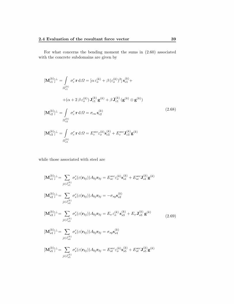
2.4 Evaluation of the resultant force vector 39
For what concerns the bending moment the sums in (2.60) associatedwith the concrete subdomains are given by
[M(k)c1 ]⊥ =
∫
Ω(k)c1
σrc r dΩ = [αε(k)
o + β (ε(k)o )2] s(k)
c1 +
+(α+ 2 β ε(k)o )J(k)
c1 g(k) + β J(k)c1 (g(k) ⊗ g(k))
[M(k)c2 ]⊥ =
∫
Ω(k)c2
σrc r dΩ = σcu s(k)
c2
[M(k)c3 ]⊥ =
∫
Ω(k)c3
σrc r dΩ = Esec
c ε(k)o s(k)
c3 + Esecc J(k)
c3 g(k)
(2.68)
while those associated with steel are
[M(k)s1 ]⊥=
∑
j∈I(k)s1
σrs(ε(rbj))Abjrbj = Esec
sc ε(k)o s(k)
s1 +Esecsc J(k)
s1 g(k)
[M(k)s2 ]⊥=
∑
j∈I(k)s2
σrs(ε(rbj))Abjrbj = −σsys
(k)s2
[M(k)s3 ]⊥=
∑
j∈I(k)s3
σrs(ε(rbj))Abjrbj = Es ε
(k)o s(k)
s3 +Es J(k)s3 g(k)
[M(k)s4 ]⊥=
∑
j∈I(k)s4
σrs(ε(rbj))Abjrbj = σsys
(k)s4
[M(k)s5 ]⊥=
∑
j∈I(k)s5
σrs(ε(rbj))Abjrbj = Esec
st ε(k)o s(k)
s5 +Esecst J(k)
s5 g(k)
(2.69)

40Ultimate Limit State analysis of RC sections subject to axial
force and biaxial bending
The third order tensor J(k)cq appearing in (2.68) is evaluated by means of
the same general formula reported in [35]:
J(k)cq =
∫
Ω(k)cq
(r⊗ r⊗ r) dΩ =120
n(k)cq∑
j=1c(k)qj [r(k)
qj ⊗ r(k)qj ⊗ r(k)
qj +
+13(r(k)
q(j+1) ⊗ r(k)qj ⊗ r(k)
qj + r(k)q(j+1) ⊗ r(k)
q(j+1) ⊗ r(k)qj +
+r(k)q(j+1) ⊗ r(k)
qj ⊗ r(k)q(j+1) + r(k)
qj ⊗ r(k)q(j+1) ⊗ r(k)
qj +
+r(k)qj ⊗ r(k)
q(j+1) ⊗ r(k)q(j+1) + r(k)
qj ⊗ r(k)qj ⊗ r(k)
q(j+1))+
+r(k)q(j+1) ⊗ r(k)
q(j+1) ⊗ r(k)q(j+1)]
(2.70)
where n(k)cq is the number of vertices of Ω(k)
cq and
c(k)qj = r(k)
qj · [r(k)q(j+1)]
⊥ =
x
(k)qj
y(k)qj
·
y
(k)q(j+1)
−x(k)q(j+1)
(2.71)
provided that the vertices of the boundary of each subdomain Ω(k)cq have been
numbered in consecutive order by circulating in counter-clockwise sense.Composition of J(k)
cq with the second-order tensor g(k) ⊗ g(k), see e.g.(2.68)1, is performed as follows:
[J(k)cq (g(k) ⊗ g(k))]i = [J(k)
cq ]ijk [g(k) ⊗ g(k)]jk (2.72)
Finally, the second area moment of the q-th steel subdomain is
J(k)sq =
∑
j∈I(k)sq
Abjrbj ⊗ rbj (2.73)
where the significance of the adopted symbols is analogous to thet employedin (2.67).

2.5 Evaluation of the matrix H(k) 41
2.5 Evaluation of the matrix H(k)
The second task to accomplish for the actual implementation of the proce-dure B is the evaluation of the matrix H(k). To this end, we start evaluatingthe tangent matrix dR(k), reported in equation (2.29), which is the Hessianof both functions φ and ψ.
Similarly to f (k)r we shall provide a set of formulas which allow us to
evaluate dR(k) as sum of separate contributions represented by terms whichare expressed solely as function of the vertices of the section and of theconstitutive parameters of the materials.
Adopting the same procedure illustrated for f (k)r we subdivide the con-
crete cross section in four subdomains Ω(k)cq for computing the integrals as-
sociated with concrete and five subsets I(k)sq for steel.
The entries of the matrix (2.29) have been evaluated as follows
∂Nr
∂εo
∣∣∣∣u(k)
=3∑
q=1
∂Ncq
∂εo
∣∣∣∣u(k)
+5∑
q=1
∂Nsq
∂εo
∣∣∣∣u(k)
(2.74)
∂Nr
∂g
∣∣∣∣u(k)
=3∑
q=1
∂Ncq
∂g
∣∣∣∣u(k)
+5∑
q=1
∂Nsq
∂g
∣∣∣∣u(k)
(2.75)
for what concerns the derivatives of the axial force Nr and
∂[Mr]⊥
∂εo
∣∣∣∣∣u(k)
=3∑
q=1
∂[Mcq]⊥
∂εo
∣∣∣∣∣u(k)
+5∑
q=1
∂[Msq]⊥
∂εo
∣∣∣∣∣u(k)
(2.76)
∂[Mr]⊥
∂g
∣∣∣∣∣u(k)
=3∑
q=1
∂[Mcq]⊥
∂g
∣∣∣∣∣u(k)
+5∑
q=1
∂[Msq]⊥
∂g
∣∣∣∣∣u(k)
(2.77)
for the derivatives of [Mr]⊥. The explicit expression of each addend in thesums above is reported in section 2.5.1.
However, it has been emphasized in section 2.3 that the tangent matrixdR(k) may be ill conditioned or singular in special situations which canoccur during the iterations of the Newton method when large compressiveor tensile axial forces are near the ultimate values corrsponding to pure axialstrain applied to the section.
For this reason the matrix H(k) used in the update formula (2.30) isobtained by suitably modifying dR(k), in order to get positive definitenessand good conditioning. To this end, the entries of H(k) are evaluated as in

42Ultimate Limit State analysis of RC sections subject to axial
force and biaxial bending
the formulas (2.74)-(2.77) above except for the derivatives of the quantitiesNs2, Ns4, [Ms2]⊥ and [Ms4]⊥ associated in turn with the horizontal plateauof the steel constitutive law.
Figure 2.9: Steel constitutive law for the evaluation of H(k)
Accordingly, a fictitious hardening constitutive law (see figure 2.9), whoseconstant slope has been numerically evaluated in order to improve the con-vergence rate of procedure B, has been assigned to the steel bars belongingto the sets I(k)
s2 and I(k)s4 . Obviously, in order to correctly evaluate the resul-
tant vector f (k)r , the stress pertaining to each bar in the sets I(k)
s2 and I(k)s4 has
been left constant and equal to −σsy and σsy respectively. For the detailsthe reader is referred to section 2.5.2.
2.5.1 Integration formulas for the evaluation of the tangentmatrix dR(k)
Aim of this section is to detail the computation of the derivatives appearingin the expressions (2.74)-(2.77) for each one of the subdomains defined in(2.57)-(2.58). In this respect we remark that the sets I(k)
sq are collections oflumped areas, so that the area moments of the steel bars belonging to thegeneric set I(k)
sq are discontinuosly dependent on ε(k)o and g(k), i.e. they are
piecewise constant. Accordingly, the derivatives of the area moments of thesteel bars are zero and will be omitted in the sequel.

2.5 Evaluation of the matrix H(k) 43
The addends of the sums in (2.74) are given by
∂Nc1
∂εo
∣∣∣∣u(k)
=(α+ 2βε(k)o )A(k)
c1 + [αε(k)o + β(ε(k)
o )2]∂Ac1
∂εo
∣∣∣∣u(k)
+
+2βs(k)c1 · g(k) + (α+ 2βε(k)
o )∂sc1
∂εo
∣∣∣∣u(k)
· g(k)+
+β∂Jc1
∂εo
∣∣∣∣u(k)
g(k) · g(k)
∂Nc2
∂εo
∣∣∣∣u(k)
=∂Ac2
∂εo
∣∣∣∣u(k)
σcu
∂Nc3
∂εo
∣∣∣∣u(k)
=Esecc A
(k)c3 + Esec
c ε(k)o
∂Ac3
∂εo
∣∣∣∣u(k)
+Esecc
∂sc3
∂εo
∣∣∣∣u(k)
g(k)
(2.78)
for concrete and
∂Ns1
∂εo
∣∣∣∣u(k)
= Esecsc A
(k)s1 ;
∂Ns2
∂εo
∣∣∣∣u(k)
= 0
∂Ns3
∂εo
∣∣∣∣u(k)
= EsA(k)s3 ;
∂Ns4
∂εo
∣∣∣∣u(k)
= 0
∂Ns5
∂εo
∣∣∣∣u(k)
= Esecst A
(k)s5
(2.79)
for steel bars.
Similarly, the derivatives in (2.75) of the axial force with respect to g

44Ultimate Limit State analysis of RC sections subject to axial
force and biaxial bending
evaluated at u(k) are given by
∂Nc1
∂g
∣∣∣∣u(k)
=(αε(k)o + β(ε(k)
o )2)∂Ac1
∂g
∣∣∣∣u(k)
+ (α+ 2βε(k)o )s(k)
c1 +
+(α+ 2βε(k)o )
[∂sc1
∂g
]T
u(k)
g(k) + 2βJ(k)c1 g(k)+
+β∂Jc1
∂g
∣∣∣∣u(k)
(g(k) ⊗ g(k))
∂Nc2
∂g
∣∣∣∣u(k)
=∂Ac2
∂g
∣∣∣∣u(k)
σcu
∂Nc3
∂g
∣∣∣∣u(k)
=Esecc ε(k)
o
∂Ac3
∂g
∣∣∣∣u(k)
+Esecc s(k)
c3 + Esecc
[∂sc3
∂g
]T
u(k)
g(k)
(2.80)
for concrete and
∂Ns1
∂g
∣∣∣∣u(k)
= Esecsc s(k)
s1 ;∂Ns2
∂g
∣∣∣∣u(k)
= 0
∂Ns3
∂g
∣∣∣∣u(k)
= Ess(k)s3 ;
∂Ns4
∂g
∣∣∣∣u(k)
= 0
∂Ns5
∂g
∣∣∣∣u(k)
= Esecst s(k)
s5
(2.81)
for steel bars. Notice that the composition of the third-order tensor [∂Jc1/∂g]u(k)
with (g(k) ⊗ g(k)) is performed as in (2.72):
[∂Jc1
∂g
∣∣∣∣u(k)
(g(k) ⊗ g(k))]
i
=[∂Jc1
∂g
∣∣∣∣u(k)
]
jli
[g(k)]j [g(k)]l =
=∂[Jc1]jl∂gi
∣∣∣∣u(k)
[g(k)]j [g(k)]l
(2.82)
The derivatives at u(k) of the three area moments Acq, scq and Jcq of thegeneric concrete subdomain Ω
(k)cq with respect to the strain parameters εo
and g can be evaluated by invoking (2.62), (2.63) and (2.64) and recallingthat each subdomain is polygonal. Actually, each subdomain Ω(k)
cq changeswith the strain parameters and the same happens for the area moments.

2.5 Evaluation of the matrix H(k) 45
- derivatives of area:
∂Acq
∂εo
∣∣∣∣u(k)
=12
n(k)cq∑
j=1
(∂rqj
∂εo
∣∣∣∣u(k)
· [r(k)q(j+1)]
⊥ +
+ r(k)qj ·
∂[rq(j+1)]⊥
∂εo
∣∣∣∣∣u(k)
)=
12
n(k)cq∑
j=1p(k)qj
∂Acq
∂g
∣∣∣∣u(k)
=12
n(k)cq∑
j=1
([∂rqj
∂g
]T
u(k)
[r(k)q(j+1)]
⊥+
+
[∂[rq(j+1)]⊥
∂g
]T
u(k)
r(k)qj
=
12
n(k)cq∑
j=1q(k)
qj
(2.83)
- derivatives of first area moment:
∂scq
∂εo
∣∣∣∣u(k)
=16
n(k)cq∑
j=1
[p(k)qj
(r(k)qj + r(k)
q(j+1)
)+
+c(k)qj
(∂rqj
∂εo
∣∣∣∣u(k)
+∂rq(j+1)
∂εo
∣∣∣∣u(k)
)]
∂scq
∂g
∣∣∣∣u(k)
=16
n(k)cq∑
j=1
[(r(k)qj + r(k)
q(j+1)
)⊗ q(k)
qj +
+ c(k)qj
(∂rqj
∂g
∣∣∣∣u(k)
+∂rq(j+1)
∂g
∣∣∣∣u(k)
)]
(2.84)

46Ultimate Limit State analysis of RC sections subject to axial
force and biaxial bending
- derivatives of second area moment:
∂Jcq
∂εo
∣∣∣∣u(k)
=112
n(k)cq∑
j=1
p(k)qj
[r(k)qj ⊗ r(k)
qj + sym(r(k)q(j+1) ⊗ r(k)
qj
)+
+r(k)q(j+1) ⊗ r(k)
q(j+1)
]+
+c(k)qj
[∂rqj
∂εo
∣∣∣∣u(k)
⊗ r(k)qj + sym
(∂rq(j+1)
∂εo
∣∣∣∣u(k)
⊗ r(k)qj
)+
+∂rq(j+1)
∂εo
∣∣∣∣u(k)
⊗ r(k)q(j+1) + r(k)
qj ⊗ ∂rqj
∂εo
∣∣∣∣u(k)
+
+sym(r(k)q(j+1) ⊗
∂rqj
∂εo
∣∣∣∣u(k)
)+ r(k)
q(j+1) ⊗∂rq(j+1)
∂εo
∣∣∣∣u(k)
]
∂Jcq
∂g
∣∣∣∣u(k)
=112
n(k)cq∑
j=1
[r(k)qj ⊗ r(k)
qj + sym(r(k)q(j+1) ⊗ r(k)
qj )+
+r(k)q(j+1) ⊗ r(k)
q(j+1)
]⊗ q(k)
qj +
+c(k)qj
[∂rqj
∂g
∣∣∣∣u(k)
⊗ r(k)qj + sym
(∂rq(j+1)
∂g
∣∣∣∣u(k)
⊗ r(k)qj
)+
+∂rq(j+1)
∂g
∣∣∣∣u(k)
⊗ r(k)q(j+1) + r(k)
qj ⊗ ∂rqj
∂g
∣∣∣∣u(k)
+
+sym(r(k)q(j+1) ⊗
∂rqj
∂g
∣∣∣∣u(k)
)+ rq(j+1) ⊗
∂rq(j+1)
∂g
∣∣∣∣u(k)
]
(2.85)
The previous formulas emphasize that the required derivatives of the areamoments depend upon the change, with respect to εo and g, of the positionvectors which define each subdomain Ω(k)
cq . Such vectors can be grouped intwo mutually disjoint subsets. The first one contains the position vectorswhich define the boundary of Ωc; accordingly their coordinates are fixed andthe relevant derivatives with respect to εo and g are trivially zero.
Therefore, we shall concentrate on the second set, denoted in the sequelby Γ
(k)cq , which collects the position vectors r(k)
qj belonging to the generic

2.5 Evaluation of the matrix H(k) 47
edge of the boundary of Ωc with the exception of the relevant end points.In other words the position vectors included in Γ (k)
cq are those which definevertices belonging to two adiacent subdomains Ω(k)
c,j and Ω(k)c,j+1 but different
from the vertices defining the boundary of Ωc.
Figure 2.10: Evaluation of the position vector r(k)qj
The derivative at u(k) of each rqj ∈ Γ(k)cq with respect to εo and g can
be derived as follows. Let ra and rb be the end vertices of the edge of thesection boundary which r(k)
qj belongs to (see figure 2.10). Thus r(k)qj can be
expressed in parametric form as
r(k)qj = ra + ϑ
(k)qj (rb − ra) (2.86)
Since r(k)qj ∈ Γ
(k)cq we can set ε(r(k)
qj ) = ε∗ where ε∗ = 0 if r(k)qj belongs to
the neutral axis i.e. r(k)qj ∈ Ω
(k)c0 ∩ Ω(k)
c1 , ε∗ = εcp if r(k)qj ∈ Ω
(k)c1 ∩ Ω(k)
c2 , and
ε∗ = εcu if r(k)qj ∈ Ω
(k)c2 ∩ Ω(k)
c3 . Thus the parameter ϑ(k)qj in (2.86) can be
evaluated explicitly as
ϑ(k)qj =
ε∗ − ε(k)a
ε(k)b − ε
(k)a
(2.87)
where
ε(k)a = ε(k)
o + g(k) · ra ε(k)b = ε(k)
o + g(k) · rb (2.88)
Notice that the case ε(k)a = ε
(k)b can be excluded since, otherwise, the
edge defined by the end vertices ra and rb would be parallel to or belong toa generic axis of constant strain subdividing two adiacent subdomains Ωc,j
and Ωc,j+1; in both cases no point of the edge belongs to Γ (k)cq .

48Ultimate Limit State analysis of RC sections subject to axial
force and biaxial bending
In conclusion, on the basis of the previous three formulas we can write
∂rqj
∂εo
∣∣∣∣u(k)
=∂ϑqj
∂εo
∣∣∣∣u(k)
(rb−ra)∂rqj
∂g
∣∣∣∣u(k)
= (rb−ra)⊗∂ϑqj
∂g
∣∣∣∣u(k)
(2.89)
where∂ϑqj
∂εo
∣∣∣∣u(k)
= − 1
ε(k)b − ε
(k)a
∂ϑqj
∂g
∣∣∣∣u(k)
=ra(ε∗ − ε
(k)b ) − rb(ε∗ − ε
(k)a )
(ε(k)b − ε
(k)a )2
(2.90)
Let us now consider the derivatives appearing in (2.76). Invoking (2.68)and (2.69) one gets:
∂[Mc1]⊥
∂εo
∣∣∣∣∣u(k)
=(α+ 2βε(k)o )s(k)
c1 + (αεo + β(ε(k)o )2)
∂sc1
∂εo
∣∣∣∣u(k)
+
+2βJ(k)c1 g(k) + (α+ 2βε(k)
o )∂Jc1
∂εo
∣∣∣∣u(k)
g(k)+
+β∂Jc1
∂εo
∣∣∣∣∣u(k)
(g(k) ⊗ g(k))
∂[Mc2]⊥
∂εo
∣∣∣∣∣u(k)
=σcu∂sc2
∂εo
∣∣∣∣u(k)
∂[Mc3]⊥
∂εo
∣∣∣∣∣u(k)
=Esecc s(k)
c3 + Esecc ε(k)
o
∂sc3
∂εo
∣∣∣∣u(k)
+ Esecc
∂Jc3
∂εo
∣∣∣∣u(k)
g(k)
(2.91)
for concrete and
∂[Ms1]⊥
∂εo
∣∣∣∣∣u(k)
= Esecsc s(k)
s1 ;∂[Ms2]⊥
∂εo
∣∣∣∣∣u(k)
= 0
∂[Ms3]⊥
∂εo
∣∣∣∣∣u(k)
= Ess(k)s3 ;
∂[Ms4]⊥
∂εo
∣∣∣∣∣u(k)
= 0
∂[Ms5]⊥
∂εo
∣∣∣∣∣u(k)
= Esecst s(k)
s5
(2.92)
for steel bars.

2.5 Evaluation of the matrix H(k) 49
Finally, the derivatives in (2.77) at u(k) of [Mcq]⊥ and [Msq]⊥ with respectto g are given by
∂[Mc1]⊥
∂g
∣∣∣∣∣u(k)
=(αε(k)o + β(ε(k)
o )2)∂sc1
∂g
∣∣∣∣u(k)
+ (α+ 2βε(k)o )J(k)
c1 +
+(α+ 2βε(k)o )
∂Jc1
∂g
∣∣∣∣u(k)
g(k) + 2βJ(k)c1 g(k)+
+β∂Jc1
∂g
∣∣∣∣∣u(k)
(g(k) ⊗ g(k))
∂[Mc2]⊥
∂g
∣∣∣∣∣u(k)
=σcu∂sc2
∂g
∣∣∣∣u(k)
∂[Mc3]⊥
∂g
∣∣∣∣∣u(k)
=Esecc ε(k)
o
∂sc3
∂g
∣∣∣∣u(k)
+Esecc J(k)
c3 + Esecc
∂Jc3
∂g
∣∣∣∣u(k)
g(k)
(2.93)
for concrete and
∂[Ms1]⊥
∂g
∣∣∣∣∣u(k)
= Esecsc J(k)
s1 ;∂[Ms2]⊥
∂g
∣∣∣∣∣u(k)
= 0
∂[Ms3]⊥
∂g
∣∣∣∣∣u(k)
= EsJ(k)s3 ;
∂[Ms4]⊥
∂g
∣∣∣∣∣u(k)
= 0
∂[Ms5]⊥
∂g
∣∣∣∣∣u(k)
= Esecst J(k)
s1
(2.94)
for steel bars.With reference to (2.93) we remark that
[∂Jcq
∂g
∣∣∣∣u(k)
g(k)]
ij
=[∂Jcq
∂g
∣∣∣∣u(k)
]
ilj
[g(k)]l =∂[Jcq]il∂gj
∣∣∣∣∣u(k)
[g(k)]l (2.95)
[∂Jcq
∂g
∣∣∣∣∣u(k)
g(k) ⊗ g(k)
]
ij
=
[∂Jcq
∂g
∣∣∣∣∣u(k)
]
ilmj
[g]l[g]m =
=∂[Jcq]ilm∂gj
∣∣∣∣∣u(k)
[g]l[g]m
(2.96)

50Ultimate Limit State analysis of RC sections subject to axial
force and biaxial bending
The third and fourth order tensor reported above can be computed asfollows
∂Jcq
∂εo
∣∣∣∣∣u(k)
=120
n(k)cq∑
j=1
p(k)qj
[r(k)qj ⊗ r(k)
qj ⊗ r(k)qj +
13
(r(k)q(j+1) ⊗ r(k)
qj ⊗ r(k)qj +
+r(k)q(j+1) ⊗ r(k)
q(j+1) ⊗ r(k)qj + r(k)
q(j+1) ⊗ r(k)qj ⊗ r(k)
q(j+1)+
+r(k)qj ⊗ r(k)
q(j+1) ⊗ r(k)qj + r(k)
qj ⊗ r(k)q(j+1) ⊗ r(k)
q(j+1)+
r(k)qj ⊗ r(k)
qj ⊗ r(k)q(j+1)
)+ r(k)
q(j+1) ⊗ r(k)q(j+1) ⊗ r(k)
q(j+1)
]+
+c(k)qj
∂
∂εo
[rqj ⊗ rqj ⊗ rqj +
13
(rq(j+1) ⊗ rqj ⊗ rqj+
+rq(j+1) ⊗ rq(j+1) ⊗ rqj + rq(j+1) ⊗ rqj ⊗ rq(j+1)+
+rqj ⊗ rq(j+1) ⊗ rqj + rqj ⊗ rq(j+1) ⊗ rq(j+1)+
rqj ⊗ rqj ⊗ rq(j+1)
)+ rq(j+1) ⊗ rq(j+1) ⊗ rq(j+1)
]
u(k)
(2.97)
where∂
∂εo(a ⊗ b⊗ c) =
∂a∂εo
⊗ b⊗ c + a ⊗ ∂b∂εo
⊗ c + a ⊗ b⊗ ∂c∂εo
.

2.5 Evaluation of the matrix H(k) 51
Finally:
∂Jcq
∂g
∣∣∣∣∣u(k)
=120
n(k)cq∑
j=1
[r(k)qj ⊗ r(k)
qj ⊗ r(k)qj +
13
(r(k)q(j+1) ⊗ r(k)
qj ⊗ r(k)qj +
+r(k)q(j+1) ⊗ r(k)
q(j+1) ⊗ r(k)qj + r(k)
q(j+1) ⊗ r(k)qj ⊗ r(k)
q(j+1)+
+r(k)qj ⊗ r(k)
q(j+1) ⊗ r(k)qj + r(k)
qj ⊗ r(k)q(j+1) ⊗ r(k)
q(j+1)+
+r(k)qj ⊗ r(k)
qj ⊗ r(k)q(j+1)
)+ r(k)
q(j+1) ⊗ r(k)q(j+1) ⊗ r(k)
q(j+1)
]⊗ q(k)
qj +
+c(k)qj
∂
∂g
[rqj ⊗ rqj ⊗ rqj +
13
(rq(j+1) ⊗ rqj ⊗ rqj+
+rq(j+1) ⊗ rq(j+1) ⊗ rqj + rq(j+1) ⊗ rqj ⊗ rq(j+1)+
+rqj ⊗ rq(j+1) ⊗ rqj + rqj ⊗ rq(j+1) ⊗ rq(j+1)+
+rqj ⊗ rqj ⊗ rq(j+1)
)+ rq(j+1) ⊗ rq(j+1) ⊗ rq(j+1)
]
u(k)
(2.98)
where∂
∂g(a⊗ b⊗ c) =
∂a∂g
⊗ b⊗ c + a ⊗ ∂b∂g
⊗ c + a ⊗ b ⊗ ∂c∂g
.
As a final remark, we draw the reader’s attention on the fact that thederivatives of Ns2 and Ns4, see e.g. formulas (2.79) and (2.81), as well as thederivatives of [Ms2]⊥ and [Ms4]⊥, formulas (2.92) and (2.94), with respectto εo and g are zero.
Farther, if the strain is εcu ≤ ε ≤ εcp over the entire concrete sectionthen Ω
(k)c1 , Ω(k)
c3 and Γ(k)cq , q = 1, 2, 3, are empty being Ω(k)
c2 ≡ Ωc, thus thederivatives of the area moments of Ω(k)
cq as well as the derivatives of Ncq and[Mcq]⊥, q = 1, 2, 3, with respect to εo and g are zero.
This motivates the necessity of modifying the tangent matrix in order toavoid singularity.

52Ultimate Limit State analysis of RC sections subject to axial
force and biaxial bending
2.5.2 Integration formulas for the evaluation of the matrixH(k)
Aim of this section is to define a proper modification for the tangent matrixin order to avoid its singularity. To this end, it is enough to replace thederivatives of the axial force and of the bending moment associated with thesteel bars pertaining to the sets I(k)
s2 and I(k)s4 with suitably defined values
which result in a positive definite matrix H(k). In this respect we define foreach bar belonging to I(k)
s2 and I(k)s4 a modified constitutive law σrm
bj havingconstant slope:
∂σrmbj (ε)∂ε
= b εsy ≤ ε ≤ εsu (2.99)
where the parameter b is defined by
b =ασsy − σsy
εsu − εsy(2.100)
Numerical experiments have been carried out by making α range in theinterval [1.0001; 1.1]. They have shown that the better performances areobtained by setting α = 1.01.
Integration of equation (2.99) leads to:
σrmbj (ε) = abj + bε εsy ≤ ε ≤ εsu (2.101)
If we wanted to evaluate R(k) using eq. (2.101), we would need to evaluatethe integration constant abj by using the condition σrm
bj [ε(k)(rbj)] = σsy . This
would ensure that the resultant f (k)r , and hence the residual R(k) in (2.28),
is not affected by the modified constitutive law (2.101) whose only purposeis to ensure a positive-definite matrix H(k) in the modified Newton method.However, the residual R(k) is always evaluated using the constitutive lows(2.26) and (2.27) and it is worth noting that the values of the integrationconstant abj are inessential in the evaluation of H(k).
To show this property we evaluate the stress resultants pertaining tothe j-th bar belonging to I(k)
s2 and I(k)s4 . On account of (2.101) the relevant
expressions are provided by
N(k)bj = σrm
bj Abj = (abj + ε(k)o b)Abj + bAbjrbj · g(k) (2.102)
[M(k)bj ]⊥ = σrm
bj Abjrbj = (abj + ε(k)o b)Abjrbj + bAbj(rbj ⊗ rbj)g(k) (2.103)

2.6 Integration formulas for the evaluation of φ 53
Thus, the relevant derivatives with respect to the strain parameters become:
∂Nbj
∂εo
∣∣∣∣∣u(k)
= bAbj ;∂Nbj
∂g
∣∣∣∣∣u(k)
= bAbjrbj
∂[Mbj]⊥
∂εo
∣∣∣∣∣u(k)
= bAbjrbj;∂[Mbj ]⊥
∂g
∣∣∣∣∣u(k)
= bAbjrbj ⊗ rbj
(2.104)
Summing up the previous contributions for all bars we finally obtain
∂Ns2
∂εo
∣∣∣∣∣u(k)
= bA(k)s2 ;
∂Ns2
∂g
∣∣∣∣∣u(k)
= bs(k)s2 ;
∂[Ms2]⊥
∂εo
∣∣∣∣∣u(k)
= bs(k)s2 ;
∂[Ms2]⊥
∂g
∣∣∣∣∣u(k)
= bJ(k)s2 ;
(2.105)
for the index set I(k)s2 and
∂Ns4
∂εo
∣∣∣∣∣u(k)
= bA(k)s4 ;
∂Ns4
∂g
∣∣∣∣∣u(k)
= bs(k)s4
∂[Ms4]⊥
∂εo
∣∣∣∣∣u(k)
= bs(k)s4 ;
∂[Ms4]⊥
∂g
∣∣∣∣∣u(k)
= bJ(k)s4
(2.106)
for the bars belonging to I(k)s4 .
The above derivatives replace the analogous quantities appearing in for-mulas (2.74)-(2.77) so that the the so obtained matrix H(k) is always positivedefinite as well as symmetric.
2.6 Integration formulas for the evaluation of φ
The expression of φ as a closed form function of the coordinates of thevertices of the subdomains defined in (2.57) and of the bars pertaining tothe subsets in (2.58) is as follows:
φ(u(k)) =3∑
q=1
φcq(u(k)) +5∑
q=1
φsq(u(k)) (2.107)

54Ultimate Limit State analysis of RC sections subject to axial
force and biaxial bending
where
φc1(u(k)) =(α
2(ε(k)
o )2 +β
3(ε(k)
o )3)A
(k)c1 +
+(α ε(k)
o + β (ε(k)o )2
)s(k)c1 · g(k)+
+(α
2+ β (ε(k)
o ))
J(k)c1 g(k) · g(k) +
β
3J(k)
c1 g(k) g(k) · g(k)
(2.108)
φc2(u(k)) =(α
2ε2cp +
β
3ε3cp
)A
(k)c2 + σco (ε(k)
o − εcp) A(k)c2 +
+σco s(k)c2 · g(k)
(2.109)
φc3(u(k)) =(α
2ε2cp +
β
3ε3cp
)A
(k)c3 + σco (εcu − εcp)A
(k)c3 +
+Esec
c
2((ε(k)
o )2 − ε2cu)A(k)c3 +
+Esecc ε(k)
o s(k)c3 · g(k) +
Esecc
2J(k)
c3 g(k) · g(k)
(2.110)
for concrete, and
φs1(u(k)) =A(k)s1
[Es
2ε2sy − σsy (εcu + εsy) +
Esecsc
2((ε(k)
o )2 − ε2cu)]+
+Esecsc ε(k)
o s(k)s1 · g(k) +
Esecsc
2J(k)
s1 g(k) · g(k)
(2.111)
φs2(u(k)) =A(k)s2
[Es
2ε2sy − σsy (ε(k)
o + εsy)]− σsy s(k)
s2 · g(k) (2.112)
φs3(u(k)) =A(k)s3
Es
2(ε(k)
o )2 + Es ε(k)o s(k)
s3 · g(k) +Es
2J(k)
s3 g(k) · g(k) (2.113)
φs4(u(k)) =A(k)s4
[Es
2ε2sy + σsy (ε(k)
o − εsy)]
+ σsy s(k)s4 · g(k) (2.114)
φs5(u(k)) =A(k)s5
[Es
2ε2sy + σsy (εsu − εsy) +
Esecst
2((ε(k)
o )2 − ε2su)]+
+Esecst ε(k)
o s(k)s5 · g(k) +
Esecst
2J(k)
s5 g(k) · g(k)
(2.115)

2.7 Numerical results 55
for the steel bars.
2.7 Numerical results
We present a comprehensive set of numerical examples which have beencarried out with the aim of testing the proposed algorithm quite intensively.
Actually, although the algorithm has been conceived with the objectiveof finding the ultimate load associated with a fixed given load fd and a givenload direction fl, it has been decided to construct the whole failure surfacefor several RC sections.
Figure 2.11: Assumption of the fixed load vector
In particular, see figure 2.11, each surface has been constructed in thespace N , Mx, My by making the load fd move along the segment definedby end points fNmax − fNmin and assuming that, for each fd, the unit vectorfl = 0, cosθ, sin θ uniformly spans the subspace Mx −My .
The vectors fNmax and fNmin are the resultant of the stress field corre-sponding to a uniform strain field εo over the section associated, respectively,with the values εo = εsy and εo = εcp.
All interaction surfaces have been constructed by considering 100 valuesof fd and, for each of them, 100 vectors fl so that the total number of analyses

56Ultimate Limit State analysis of RC sections subject to axial
force and biaxial bending
carried out for each surface has an order of magnitude equal to 104.Several tipology of RC sections have been analyzed with the aim of con-
sidering a representative set of the most typical shapes encountered in build-ings, precast sheds and bridge piers. In this section we present numerical re-sults obtained for rectangular, L-shaped, multicell , T-shaped and Y-shapedsections.
Geometric data and reinforcement pattern for each of them are reportedin figures 2.12, 2.13(a), 2.15, 2.16 and 2.17 wherein Rck is the characteristiccompressive cubical strength of concrete. The value Rck = 25N/mm2 hasbeen used in all examples. In accordance with [33, 39], the correspondingvalue of fck is 20.75N/mm2.
The numerical performances of the solution algorithm are also suppliedin table 2.1 which reports the minimum, maximum and average number ofiterations necessary to achieve convergence in each of the separate iterativeprocedures namely:
- the iterative procedure used to evaluate λ∗;- the iterative procedure used to evaluate u(f);- the line-search (L-S) procedure.
Rectangular L-shaped MulticellAvg Min Max Avg Min Max Avg Min Max
λ∗ 13.2 5 30 12.7 5 30 12.4 6 30u(fi) 6.72 2 26 6.65 2 392 6.94 1 57L-S 0.121 0 59 0.138 0 26 0.105 0 27
T-shaped Y-shapedAvg Min Max Avg Min Max
λ∗ 13.1 5 30 12.6 5 30u(fi) 6.68 2 96 6.78 2 78L-S 0.129 0 30 0.098 0 14
Table 2.1: Number of iterations for the construction of the failure surfaces(100× 100) of the rectangular, L-shaped, multicell, T-shaped and Y-shapedsections
In this respect we remind that the second iterative procedure is invokedat each single iteration of the first one and that, if necessary, the thirditerative procedure is adopted within a single iteration of the second one.In particular the average number of L-S iterations reported in the table isby far less than 1; this confirms that the L-S procedure is actually resortedto only occasionally.

2.7 Numerical results 57
In order to show the convergence rates of the proposed algorithm we plotthe average number of iterations needed by the two iterative procedures inorder to achieve convergence as a function of the values assigned to tole andtolR. Figure 2.14(b) numerically shows that procedure B is superlinearlyconvergent. Such result was expected because procedure B consists in aslight modification of the Newton method which is quadratically convergent.Conversely, procedure A is based upon a simpler iterative algorithm and,see figure 2.14(a), does not exhibit a rate of convergence as good as the oneof procedure B.
Finally, we suggest to adopt the values tole = 10−5 and tolR = 10−5
which were actually employed to construct the interaction surface above,since they represent a reasonable compromise between accuracy of the resultand computational burden.
Furthermore, tables 2.4, 2.5, 2.6, 2.7 and 2.8 report, for each section, thepoints of the relevant failure surface determined assuming 12 values of fdand, for each of them, 12 vectors fl.
To provide further insights in the proposed numerical algorithm we reportthe sequence of load amplifiers λi and relevant errors ei generated for twodifferent sections. In the first case fd = 0, while in the second case both fdand fl are non null. We further specify that, in the following, axial forcesare expressed in Mega-Newton and bending moments in MNm.
The first case refers to the rectangular section of figure 2.12 in which thevector fT
e = −0.65, −0.051, −0.082. Being fl = fe we are looking for theload amplifier λ > 0 which proportionally increases fe till reaching the ULSfor the section. The ultimate load is (f∗)T = −0.7178, −0.0563, −0.0906and the load amplifier is λ∗ = 1.104340; the value of λ∗ slightly greater than1 means that the external load vector fe lies very close to the interactionsurface and within the admissible domain. The relevant results are reportedin table 2.2.
Let us now considerate the multi-cell section of figure 2.15 and supposethat the external forces associated with dead load, e.g. self-weight andpermanent loads, are kept fixed and equal to fT
d = −1.50, 1.90,−3.60.Assuming that the external forces due to live load are equal to fT
l =−6.00, 3.40, 5.30 we want to know the degree of safety of the load fe =fd+fl when only the live load are increased, i.e. when we increase fe along fl.We obtain in this case the results reported in table 2.3, with λ∗ = 2.104311.

58Ultimate Limit State analysis of RC sections subject to axial
force and biaxial bending
λi ei0.000000 +1.00E+002.479895 -2.97E+000.624736 +6.47E-010.956791 +3.38E-011.112499 -3.37E-021.098371 +2.36E-021.104184 +6.29E-041.104336 +1.54E-051.104340 +3.75E-07
Table 2.2: Iterations of Procedure B for the rectangular section subjectto fd = 0, 0, 0 and fl = −0.65,−0.051,−0.082
λi ei0.000000 +7.98E-011.659495 +4.79E-014.146055 -2.88E+002.013478 +1.75E-012.135631 -8.39E-022.096068 +2.12E-022.104048 +6.94E-042.104307 +1.03E-052.104311 +1.50E-07
Table 2.3: Iterations of Procedure B for the multicell section subject tofd = −1.50, 1.90,−3.60 and fl = −6.00, 3.40, 5.30
Concrete:Rck = 25 N/mm2
fck = 20.75 N/mm2
Steel: FeB38Kfyk = 375 N/mm2
φ 14 at the cornersφ 14 on the faces
Figure 2.12: Rectangular section

2.7 Numerical results 59
N [MN] Mx [MNm] My [MNm] N [MN] Mx [MNm] My [MNm]
0.1701 -0.0134 -0.0225 -0.0111 0.0029 -0.04150.1701 0.0058 -0.0185 -0.0111 0.0363 -0.03310.1701 0.0068 0.0000 -0.0111 0.0462 0.00000.1701 0.0058 0.0185 -0.0111 0.0363 0.03310.1701 -0.0134 0.0225 -0.0111 0.0029 0.04150.1701 -0.0264 0.0227 -0.0111 -0.0211 0.04380.1701 -0.0395 0.0227 -0.0111 -0.0464 0.04380.1701 -0.0639 0.0217 -0.0111 -0.0862 0.03760.1701 -0.0714 0.0000 -0.0111 -0.1094 0.00000.1701 -0.0639 -0.0217 -0.0111 -0.0862 -0.03760.1701 -0.0395 -0.0227 -0.0111 -0.0464 -0.04380.1701 -0.0264 -0.0227 -0.0111 -0.0211 -0.0438
-0.1924 0.0162 -0.0555 -0.3736 0.0277 -0.0662-0.1924 0.0582 -0.0427 -0.3736 0.0742 -0.0489-0.1924 0.0846 0.0000 -0.3736 0.1213 0.0000-0.1924 0.0582 0.0427 -0.3736 0.0742 0.0489-0.1924 0.0162 0.0555 -0.3736 0.0277 0.0662-0.1924 -0.0158 0.0608 -0.3736 -0.0105 0.0739-0.1924 -0.0503 0.0598 -0.3736 -0.0510 0.0700-0.1924 -0.0953 0.0459 -0.3736 -0.0992 0.0512-0.1924 -0.1413 0.0000 -0.3736 -0.1621 0.0000-0.1924 -0.0953 -0.0459 -0.3736 -0.0992 -0.0512-0.1924 -0.0503 -0.0598 -0.3736 -0.0510 -0.0700-0.1924 -0.0158 -0.0608 -0.3736 -0.0105 -0.0739
-0.5549 0.0372 -0.0736 -0.7361 0.0444 -0.0768-0.5549 0.0868 -0.0531 -0.7361 0.0966 -0.0558-0.5549 0.1495 0.0000 -0.7361 0.1669 0.0000-0.5549 0.0868 0.0531 -0.7361 0.0966 0.0558-0.5549 0.0372 0.0736 -0.7361 0.0444 0.0768-0.5549 -0.0053 0.0825 -0.7361 0.0000 0.0856-0.5549 -0.0482 0.0743 -0.7361 -0.0434 0.0751-0.5549 -0.0986 0.0539 -0.7361 -0.0940 0.0543-0.5549 -0.1728 0.0000 -0.7361 -0.1702 0.0000-0.5549 -0.0986 -0.0539 -0.7361 -0.0940 -0.0543-0.5549 -0.0482 -0.0743 -0.7361 -0.0434 -0.0751-0.5549 -0.0053 -0.0825 -0.7361 0.0000 -0.0856

60Ultimate Limit State analysis of RC sections subject to axial
force and biaxial bending
N [MN] Mx [MNm] My [MNm] N [MN] Mx [MNm] My [MNm]
-0.9174 0.0500 -0.0774 -1.0986 0.0525 -0.0726-0.9174 0.1029 -0.0564 -1.0986 0.1035 -0.0537-0.9174 0.1741 0.0000 -1.0986 0.1669 0.0000-0.9174 0.1029 0.0564 -1.0986 0.1035 0.0537-0.9174 0.0500 0.0774 -1.0986 0.0525 0.0726-0.9174 0.0053 0.0830 -1.0986 0.0105 0.0761-0.9174 -0.0369 0.0731 -1.0986 -0.0285 0.0676-0.9174 -0.0856 0.0524 -1.0986 -0.0737 0.0486-0.9174 -0.1495 0.0000 -1.0986 -0.1268 0.0000-0.9174 -0.0856 -0.0524 -1.0986 -0.0737 -0.0486-0.9174 -0.0369 -0.0731 -1.0986 -0.0285 -0.0676-0.9174 0.0053 -0.0830 -1.0986 0.0105 -0.0761
-1.2799 0.0530 -0.0645 -1.4611 0.0515 -0.0526-1.2799 0.0994 -0.0482 -1.4611 0.0911 -0.0404-1.2799 0.1502 0.0000 -1.4611 0.1280 0.0000-1.2799 0.0994 0.0482 -1.4611 0.0911 0.0404-1.2799 0.0530 0.0645 -1.4611 0.0515 0.0526-1.2799 0.0158 0.0668 -1.4611 0.0211 0.0545-1.2799 -0.0187 0.0598 -1.4611 -0.0074 0.0494-1.2799 -0.0594 0.0434 -1.4611 -0.0422 0.0365-1.2799 -0.1013 0.0000 -1.4611 -0.0719 0.0000-1.2799 -0.0594 -0.0434 -1.4611 -0.0422 -0.0365-1.2799 -0.0187 -0.0598 -1.4611 -0.0074 -0.0494-1.2799 0.0158 -0.0668 -1.4611 0.0211 -0.0545
-1.6424 0.0479 -0.0373 -1.8236 0.0426 -0.0190-1.6424 0.0784 -0.0301 -1.8236 0.0588 -0.0157-1.6424 0.0988 0.0000 -1.8236 0.0654 0.0000-1.6424 0.0784 0.0301 -1.8236 0.0588 0.0157-1.6424 0.0479 0.0373 -1.8236 0.0426 0.0190-1.6424 0.0264 0.0382 -1.8236 0.0316 0.0193-1.6424 0.0058 0.0355 -1.8236 0.0209 0.0186-1.6424 -0.0213 0.0275 -1.8236 0.0050 0.0154-1.6424 -0.0379 0.0000 -1.8236 -0.0034 0.0000-1.6424 -0.0213 -0.0275 -1.8236 0.0050 -0.0154-1.6424 0.0058 -0.0355 -1.8236 0.0209 -0.0186-1.6424 0.0264 -0.0382 -1.8236 0.0316 -0.0193
N,Mx,Mymax = 0.3514, −0.0316, 0.0000N,Mx,Mymin = −2.0049, 0.0316, 0.0000
Table 2.4: Failure surface points (12×12) of the rectangular section of figure2.12

2.7 Numerical results 61
Concrete:σcu = 12.97N/mm2
Reinforcement bars:σsy = 326N/mm2
φ24 at the cornersφ20 on the faces
(equally spaced betweenthe bars at the corners)
concrete cover: 3cm
(a) L-shaped section
(b) Failure surface of the L-shaped section
Figure 2.13: L-shaped section: geometry and failure surface

62Ultimate Limit State analysis of RC sections subject to axial
force and biaxial bending
(a) # iterations vs. tole (Procedure A)
(b) # iterations vs. tolR (Procedure B)
Figure 2.14: Average number of iterations vs. tolerance for the L-shapedsection

2.7 Numerical results 63
N [MN] Mx [MNm] My [MNm] N [MN] Mx [MNm] My [MNm]
0.3513 0.0239 -0.0623 0.0469 0.0569 -0.11530.3513 0.0518 -0.0394 0.0469 0.1040 -0.06770.3513 0.0544 -0.0038 0.0469 0.1165 -0.00310.3513 0.0545 0.0333 0.0469 0.1168 0.06890.3513 0.0450 0.0912 0.0469 0.0916 0.16930.3513 -0.0098 0.0742 0.0469 -0.0079 0.14350.3513 -0.0425 0.0527 0.0469 -0.0684 0.10190.3513 -0.0713 0.0317 0.0469 -0.1113 0.05660.3513 -0.1047 -0.0038 0.0469 -0.1638 -0.00310.3513 -0.0986 -0.0551 0.0469 -0.1613 -0.09160.3513 -0.0438 -0.0626 0.0469 -0.0750 -0.11930.3513 -0.0098 -0.0626 0.0469 -0.0079 -0.1207
-0.2575 0.0768 -0.1455 -0.5619 0.0905 -0.1650-0.2575 0.1373 -0.0850 -0.5619 0.1630 -0.0979-0.2575 0.1681 -0.0023 -0.5619 0.2057 -0.0015-0.2575 0.1709 0.0998 -0.5619 0.2145 0.1246-0.2575 0.1225 0.2200 -0.5619 0.1351 0.2393-0.2575 -0.0059 0.1916 -0.5619 -0.0039 0.2143-0.2575 -0.0842 0.1333 -0.5619 -0.0964 0.1587-0.2575 -0.1415 0.0760 -0.5619 -0.1645 0.0912-0.2575 -0.2076 -0.0023 -0.5619 -0.2331 -0.0015-0.2575 -0.2094 -0.1198 -0.5619 -0.2431 -0.1396-0.2575 -0.1019 -0.1686 -0.5619 -0.1211 -0.2044-0.2575 -0.0059 -0.1737 -0.5619 -0.0039 -0.2103
-0.8662 0.1000 -0.1773 -1.1706 0.1041 -0.1803-0.8662 0.1768 -0.1040 -1.1706 0.1791 -0.1034-0.8662 0.2298 -0.0008 -1.1706 0.2447 0.0000-0.8662 0.2499 0.1447 -1.1706 0.2749 0.1587-0.8662 0.1374 0.2406 -1.1706 0.1332 0.2308-0.8662 -0.0020 0.2282 -1.1706 0.0000 0.2293-0.8662 -0.1043 0.1765 -1.1706 -0.1051 0.1821-0.8662 -0.1775 0.1006 -1.1706 -0.1819 0.1050-0.8662 -0.2456 -0.0008 -1.1706 -0.2412 0.0000-0.8662 -0.2663 -0.1534 -1.1706 -0.2700 -0.1559-0.8662 -0.1341 -0.2296 -1.1706 -0.1400 -0.2426-0.8662 -0.0020 -0.2274 -1.1706 0.0000 -0.2350

64Ultimate Limit State analysis of RC sections subject to axial
force and biaxial bending
N [MN] Mx [MNm] My [MNm] N [MN] Mx [MNm] My [MNm]
-1.4750 0.1010 -0.1708 -1.7794 0.0946 -0.1554-1.4750 0.1762 -0.0998 -1.7794 0.1642 -0.0910-1.4750 0.2497 0.0008 -1.7794 0.2412 0.0015-1.4750 0.2783 0.1603 -1.7794 0.2574 0.1479-1.4750 0.1265 0.2164 -1.7794 0.1164 0.1964-1.4750 0.0020 0.2174 -1.7794 0.0039 0.1986-1.4750 -0.1020 0.1808 -1.7794 -0.0938 0.1708-1.4750 -0.1773 0.1042 -1.7794 -0.1651 0.0991-1.4750 -0.2277 0.0008 -1.7794 -0.2053 0.0015-1.4750 -0.2521 -0.1459 -1.7794 -0.2241 -0.1301-1.4750 -0.1420 -0.2486 -1.7794 -0.1402 -0.2481-1.4750 0.0020 -0.2344 -1.7794 0.0039 -0.2210
-2.0838 0.0850 -0.1347 -2.3881 0.0722 -0.1083-2.0838 0.1459 -0.0786 -2.3881 0.1220 -0.0629-2.0838 0.2184 0.0023 -2.3881 0.1851 0.0031-2.0838 0.2247 0.1286 -2.3881 0.1844 0.1050-2.0838 0.1026 0.1698 -2.3881 0.0844 0.1357-2.0838 0.0059 0.1731 -2.3881 0.0079 0.1402-2.0838 -0.0803 0.1516 -2.3881 -0.0632 0.1261-2.0838 -0.1446 0.0892 -2.3881 -0.1168 0.0750-2.0838 -0.1758 0.0023 -2.3881 -0.1380 0.0031-2.0838 -0.1881 -0.1097 -2.3881 -0.1433 -0.0842-2.0838 -0.1345 -0.2408 -2.3881 -0.1161 -0.2117-2.0838 0.0059 -0.1942 -2.3881 0.0079 -0.1584
-2.6925 0.0557 -0.0757 -2.9969 0.0355 -0.0365-2.6925 0.0918 -0.0435 -2.9969 0.0549 -0.0203-2.6925 0.1401 0.0038 -2.9969 0.0815 0.0046-2.6925 0.1355 0.0764 -2.9969 0.0756 0.0414-2.6925 0.0620 0.0942 -2.9969 0.0381 0.0501-2.6925 0.0098 0.0991 -2.9969 0.0118 0.0522-2.6925 -0.0421 0.0938 -2.9969 -0.0157 0.0522-2.6925 -0.0817 0.0567 -2.9969 -0.0382 0.0334-2.6925 -0.0927 0.0038 -2.9969 -0.0410 0.0046-2.6925 -0.0929 -0.0555 -2.9969 -0.0413 -0.0261-2.6925 -0.0821 -0.1554 -2.9969 -0.0367 -0.0795-2.6925 0.0098 -0.1131 -2.9969 0.0118 -0.0566
N,Mx,Mymax = 0.6556, −0.0118, −0.0046N,Mx,Mymin = −3.3013, 0.0118, 0.0046
Table 2.5: Failure surface points (12× 12) of the L-shaped section of figure2.13(a)

2.7 Numerical results 65
Concrete:Rck = 25 N/mm2
fck = 20.75 N/mm2
Steel: FeB38Kfyk = 375 N/mm2
φ 32 at the cornersφ 32 on the faces
Figure 2.15: Multicell section
Concrete:Rck = 25 N/mm2
fck = 20.75 N/mm2
Steel: FeB38Kfyk = 375 N/mm2
φ 16 at the cornersφ 16 on the faces
Figure 2.16: T-shaped section

66Ultimate Limit State analysis of RC sections subject to axial
force and biaxial bending
N [MN] Mx [MNm] My [MNm] N [MN] Mx [MNm] My [MNm]
9.6567 2.1814 -3.7782 5.6762 3.9334 -6.81299.6567 2.5589 -1.4774 5.6762 4.8797 -2.81739.6567 2.6438 0.0000 5.6762 5.0050 0.00009.6567 2.5589 1.4774 5.6762 4.8797 2.81739.6567 2.1814 3.7782 5.6762 3.9334 6.81299.6567 0.0000 4.5735 5.6762 0.0000 8.84909.6567 -2.1814 3.7782 5.6762 -3.9334 6.81299.6567 -2.5589 1.4774 5.6762 -4.8797 2.81739.6567 -2.6438 0.0000 5.6762 -5.0050 0.00009.6567 -2.5589 -1.4774 5.6762 -4.8797 -2.81739.6567 -2.1814 -3.7782 5.6762 -3.9334 -6.81299.6567 0.0000 -4.5735 5.6762 0.0000 -8.8490
1.6957 5.1682 -8.9515 -2.2848 5.9269 -10.26561.6957 6.8784 -3.9712 -2.2848 8.3523 -4.82221.6957 7.2012 0.0000 -2.2848 9.0616 0.00001.6957 6.8784 3.9712 -2.2848 8.3523 4.82221.6957 5.1682 8.9515 -2.2848 5.9269 10.26561.6957 0.0000 12.6536 -2.2848 0.0000 15.27851.6957 -5.1682 8.9515 -2.2848 -5.9269 10.26561.6957 -6.8784 3.9712 -2.2848 -8.3523 4.82221.6957 -7.2012 0.0000 -2.2848 -9.0616 0.00001.6957 -6.8784 -3.9712 -2.2848 -8.3523 -4.82221.6957 -5.1682 -8.9515 -2.2848 -5.9269 -10.26561.6957 0.0000 -12.6536 -2.2848 0.0000 -15.2785
-6.2653 6.3460 -10.9916 -10.2458 6.4795 -11.2227-6.2653 9.3005 -5.3696 -10.2458 9.6620 -5.5784-6.2653 10.4881 0.0000 -10.2458 11.1203 0.0000-6.2653 9.3005 5.3696 -10.2458 9.6620 5.5784-6.2653 6.3460 10.9916 -10.2458 6.4795 11.2227-6.2653 0.0000 16.5227 -10.2458 0.0000 16.8922-6.2653 -6.3460 10.9916 -10.2458 -6.4795 11.2227-6.2653 -9.3005 5.3696 -10.2458 -9.6620 5.5784-6.2653 -10.4881 0.0000 -10.2458 -11.1203 0.0000-6.2653 -9.3005 -5.3696 -10.2458 -9.6620 -5.5784-6.2653 -6.3460 -10.9916 -10.2458 -6.4795 -11.2227-6.2653 0.0000 -16.5227 -10.2458 0.0000 -16.8922

2.7 Numerical results 67
N [MN] Mx [MNm] My [MNm] N [MN] Mx [MNm] My [MNm]
-14.2263 6.3306 -10.9649 -18.2068 5.9188 -10.2516-14.2263 9.4080 -5.4317 -18.2068 8.6489 -4.9935-14.2263 10.8522 0.0000 -18.2068 9.8212 0.0000-14.2263 9.4080 5.4317 -18.2068 8.6489 4.9935-14.2263 6.3306 10.9649 -18.2068 5.9188 10.2516-14.2263 0.0000 16.6564 -18.2068 0.0000 15.5413-14.2263 -6.3306 10.9649 -18.2068 -5.9188 10.2516-14.2263 -9.4080 5.4317 -18.2068 -8.6489 4.9935-14.2263 -10.8522 0.0000 -18.2068 -9.8212 0.0000-14.2263 -9.4080 -5.4317 -18.2068 -8.6489 -4.9935-14.2263 -6.3306 -10.9649 -18.2068 -5.9188 -10.2516-14.2263 0.0000 -16.6564 -18.2068 0.0000 -15.5413
-22.1873 5.2693 -9.1268 -26.1678 4.4128 -7.6432-22.1873 7.5233 -4.3436 -26.1678 6.0426 -3.4887-22.1873 8.2538 0.0000 -26.1678 6.4791 0.0000-22.1873 7.5233 4.3436 -26.1678 6.0426 3.4887-22.1873 5.2693 9.1268 -26.1678 4.4128 7.6432-22.1873 0.0000 13.5704 -26.1678 0.0000 11.1254-22.1873 -5.2693 9.1268 -26.1678 -4.4128 7.6432-22.1873 -7.5233 4.3436 -26.1678 -6.0426 3.4887-22.1873 -8.2538 0.0000 -26.1678 -6.4791 0.0000-22.1873 -7.5233 -4.3436 -26.1678 -6.0426 -3.4887-22.1873 -5.2693 -9.1268 -26.1678 -4.4128 -7.6432-22.1873 0.0000 -13.5704 -26.1678 0.0000 -11.1254
-30.1483 3.2638 -5.6530 -34.1288 1.7544 -3.0387-30.1483 4.2420 -2.4491 -34.1288 2.1764 -1.2565-30.1483 4.4113 0.0000 -34.1288 2.2424 0.0000-30.1483 4.2420 2.4491 -34.1288 2.1764 1.2565-30.1483 3.2638 5.6530 -34.1288 1.7544 3.0387-30.1483 0.0000 7.8305 -34.1288 0.0000 3.9778-30.1483 -3.2638 5.6530 -34.1288 -1.7544 3.0387-30.1483 -4.2420 2.4491 -34.1288 -2.1764 1.2565-30.1483 -4.4113 0.0000 -34.1288 -2.2424 0.0000-30.1483 -4.2420 -2.4491 -34.1288 -2.1764 -1.2565-30.1483 -3.2638 -5.6530 -34.1288 -1.7544 -3.0387-30.1483 0.0000 -7.8305 -34.1288 0.0000 -3.9778
N,Mx,Mymax = 13.6372, 0.0000, 0.0000N,Mx, Mymin = −38.1093, 0.0000, 0.0000
Table 2.6: Failure surface points (12 × 12) of the multicell section of figure2.15

68Ultimate Limit State analysis of RC sections subject to axial
force and biaxial bending
N [MN] Mx [MNm] My [MNm] N [MN] Mx [MNm] My [MNm]
0.5007 -0.0048 -0.0655 0.1491 0.0373 -0.12370.5007 0.0331 -0.0437 0.1491 0.1045 -0.08000.5007 0.0629 0.0000 0.1491 0.1765 0.00000.5007 0.0331 0.0437 0.1491 0.1045 0.08000.5007 -0.0048 0.0655 0.1491 0.0373 0.12370.5007 -0.0426 0.0854 0.1491 -0.0341 0.15980.5007 -0.1054 0.1088 0.1491 -0.1414 0.18580.5007 -0.1228 0.0463 0.1491 -0.1875 0.08860.5007 -0.1235 0.0000 0.1491 -0.1950 0.00000.5007 -0.1228 -0.0463 0.1491 -0.1875 -0.08860.5007 -0.1054 -0.1088 0.1491 -0.1414 -0.18580.5007 -0.0426 -0.0854 0.1491 -0.0341 -0.1598
-0.2025 0.0750 -0.1742 -0.5541 0.1069 -0.2147-0.2025 0.1654 -0.1103 -0.5541 0.2179 -0.1356-0.2025 0.2792 0.0000 -0.5541 0.3376 0.0000-0.2025 0.1654 0.1103 -0.5541 0.2179 0.1356-0.2025 0.0750 0.1742 -0.5541 0.1069 0.2147-0.2025 -0.0256 0.2152 -0.5541 -0.0170 0.2525-0.2025 -0.1579 0.2291 -0.5541 -0.1605 0.2485-0.2025 -0.2422 0.1251 -0.5541 -0.2817 0.1528-0.2025 -0.2587 0.0000 -0.5541 -0.3097 0.0000-0.2025 -0.2422 -0.1251 -0.5541 -0.2817 -0.1528-0.2025 -0.1579 -0.2291 -0.5541 -0.1605 -0.2485-0.2025 -0.0256 -0.2152 -0.5541 -0.0170 -0.2525
-0.9057 0.1310 -0.2417 -1.2572 0.1500 -0.2599-0.9057 0.2577 -0.1537 -1.2572 0.2847 -0.1644-0.9057 0.3661 0.0000 -1.2572 0.3652 0.0000-0.9057 0.2577 0.1537 -1.2572 0.2847 0.1644-0.9057 0.1310 0.2417 -1.2572 0.1500 0.2599-0.9057 -0.0085 0.2757 -1.2572 0.0000 0.2822-0.9057 -0.1547 0.2533 -1.2572 -0.1396 0.2418-0.9057 -0.2945 0.1651 -1.2572 -0.2795 0.1614-0.9057 -0.3472 0.0000 -1.2572 -0.3715 0.0000-0.9057 -0.2945 -0.1651 -1.2572 -0.2795 -0.1614-0.9057 -0.1547 -0.2533 -1.2572 -0.1396 -0.2418-0.9057 -0.0085 -0.2757 -1.2572 0.0000 -0.2822

2.7 Numerical results 69
N [MN] Mx [MNm] My [MNm] N [MN] Mx [MNm] My [MNm]
-1.6088 0.1633 -0.2681 -1.9604 0.1686 -0.2626-1.6088 0.2985 -0.1674 -1.9604 0.2864 -0.1555-1.6088 0.3420 0.0000 -1.9604 0.3127 0.0000-1.6088 0.2985 0.1674 -1.9604 0.2864 0.1555-1.6088 0.1633 0.2681 -1.9604 0.1686 0.2626-1.6088 0.0085 0.2790 -1.9604 0.0170 0.2548-1.6088 -0.1213 0.2249 -1.9604 -0.1000 0.2028-1.6088 -0.2486 0.1485 -1.9604 -0.2128 0.1327-1.6088 -0.3802 0.0000 -1.9604 -0.3720 0.0000-1.6088 -0.2486 -0.1485 -1.9604 -0.2128 -0.1327-1.6088 -0.1213 -0.2249 -1.9604 -0.1000 -0.2028-1.6088 0.0085 -0.2790 -1.9604 0.0170 -0.2548
-2.3120 0.1677 -0.2462 -2.6636 0.1552 -0.2097-2.3120 0.2563 -0.1332 -2.6636 0.2165 -0.1053-2.3120 0.2740 0.0000 -2.6636 0.2235 0.0000-2.3120 0.2563 0.1332 -2.6636 0.2165 0.1053-2.3120 0.1677 0.2462 -2.6636 0.1552 0.2097-2.3120 0.0256 0.2206 -2.6636 0.0341 0.1792-2.3120 -0.0752 0.1745 -2.6636 -0.0462 0.1391-2.3120 -0.1720 0.1141 -2.6636 -0.1250 0.0918-2.3120 -0.3155 0.0000 -2.6636 -0.2420 0.0000-2.3120 -0.1720 -0.1141 -2.6636 -0.1250 -0.0918-2.3120 -0.0752 -0.1745 -2.6636 -0.0462 -0.1391-2.3120 0.0256 -0.2206 -2.6636 0.0341 -0.1792
-3.0152 0.1350 -0.1601 -3.3668 0.1030 -0.0898-3.0152 0.1668 -0.0717 -3.3668 0.1095 -0.0337-3.0152 0.1667 0.0000 -3.3668 0.1096 0.0000-3.0152 0.1668 0.0717 -3.3668 0.1095 0.0337-3.0152 0.1350 0.1601 -3.3668 0.1030 0.0898-3.0152 0.0426 0.1293 -3.3668 0.0511 0.0689-3.0152 -0.0135 0.0972 -3.3668 0.0212 0.0519-3.0152 -0.0706 0.0653 -3.3668 -0.0085 0.0345-3.0152 -0.1555 0.0000 -3.3668 -0.0535 0.0000-3.0152 -0.0706 -0.0653 -3.3668 -0.0085 -0.0345-3.0152 -0.0135 -0.0972 -3.3668 0.0212 -0.0519-3.0152 0.0426 -0.1293 -3.3668 0.0511 -0.0689
N,Mx,Mymax = 0.8523, −0.0511, 0.0000N,Mx,Mymin = −3.7184, 0.0511, 0.0000
Table 2.7: Failure surface points (12× 12) of the T-shaped section of figure2.16

70Ultimate Limit State analysis of RC sections subject to axial
force and biaxial bending
Concrete:Rck = 40 N/mm2
fck = 33.2 N/mm2
Steel: FeB44Kfyk = 430 N/mm2
φ 16 at the cornersφ 16 on the faces
Figure 2.17: Y-shaped section

2.7 Numerical results 71
N [MN] Mx [MNm] My [MNm] N [MN] Mx [MNm] My [MNm]
1.0972 0.2155 -0.2525 0.4242 0.3325 -0.47921.0972 0.3522 -0.1631 0.4242 0.5841 -0.30501.0972 0.5497 0.0000 0.4242 0.9824 0.00001.0972 0.3522 0.1631 0.4242 0.5841 0.30501.0972 0.2155 0.2525 0.4242 0.3325 0.47921.0972 0.0697 0.3474 0.4242 0.0558 0.64911.0972 -0.2024 0.4714 0.4242 -0.4281 0.83811.0972 -0.2041 0.1581 0.4242 -0.4685 0.30271.0972 -0.2044 0.0000 0.4242 -0.4715 0.00001.0972 -0.2041 -0.1581 0.4242 -0.4685 -0.30271.0972 -0.2024 -0.4714 0.4242 -0.4281 -0.83811.0972 0.0697 -0.3474 0.4242 0.0558 -0.6491
-0.2488 0.4306 -0.6733 -0.9218 0.5052 -0.8267-0.2488 0.7788 -0.4255 -0.9218 0.9376 -0.5252-0.2488 1.2862 0.0000 -0.9218 1.4468 0.0000-0.2488 0.7788 0.4255 -0.9218 0.9376 0.5252-0.2488 0.4306 0.6733 -0.9218 0.5052 0.8267-0.2488 0.0418 0.8649 -0.9218 0.0279 0.9808-0.2488 -0.5170 0.9680 -0.9218 -0.5491 0.9994-0.2488 -0.7025 0.4298 -0.9218 -0.8934 0.5319-0.2488 -0.7237 0.0000 -0.9218 -0.9493 0.0000-0.2488 -0.7025 -0.4298 -0.9218 -0.8934 -0.5319-0.2488 -0.5170 -0.9680 -0.9218 -0.5491 -0.9994-0.2488 0.0418 -0.8649 -0.9218 0.0279 -0.9808
-1.5948 0.5531 -0.9338 -2.2678 0.5767 -0.9988-1.5948 1.0388 -0.5917 -2.2678 1.0804 -0.6238-1.5948 1.4421 0.0000 -2.2678 1.3213 0.0000-1.5948 1.0388 0.5917 -2.2678 1.0804 0.6238-1.5948 0.5531 0.9338 -2.2678 0.5767 0.9988-1.5948 0.0139 1.0435 -2.2678 0.0000 1.0575-1.5948 -0.5524 0.9809 -2.2678 -0.5329 0.9230-1.5948 -1.0169 0.5952 -2.2678 -1.0410 0.6010-1.5948 -1.1557 0.0000 -2.2678 -1.3380 0.0000-1.5948 -1.0169 -0.5952 -2.2678 -1.0410 -0.6010-1.5948 -0.5524 -0.9809 -2.2678 -0.5329 -0.9230-1.5948 0.0139 -1.0435 -2.2678 0.0000 -1.0575

72Ultimate Limit State analysis of RC sections subject to axial
force and biaxial bending
N [MN] Mx [MNm] My [MNm] N [MN] Mx [MNm] My [MNm]
-2.9408 0.5853 -1.0379 -3.6138 0.5716 -1.0383-2.9408 1.0554 -0.6174 -3.6138 0.9508 -0.5651-2.9408 1.1771 0.0000 -3.6138 1.0087 0.0000-2.9408 1.0554 0.6174 -3.6138 0.9508 0.5651-2.9408 0.5853 1.0379 -3.6138 0.5716 1.0383-2.9408 -0.0139 1.0214 -3.6138 -0.0279 0.9359-2.9408 -0.5015 0.8445 -3.6138 -0.4607 0.7497-2.9408 -0.9774 0.5563 -3.6138 -0.8860 0.4954-2.9408 -1.4713 0.0000 -3.6138 -1.5133 0.0000-2.9408 -0.9774 -0.5563 -3.6138 -0.8860 -0.4954-2.9408 -0.5015 -0.8445 -3.6138 -0.4607 -0.7497-2.9408 -0.0139 -1.0214 -3.6138 -0.0279 -0.9359
-4.2868 0.5364 -1.0016 -4.9598 0.4625 -0.8978-4.2868 0.7869 -0.4785 -4.9598 0.5995 -0.3783-4.2868 0.8160 0.0000 -4.9598 0.6014 0.0000-4.2868 0.7869 0.4785 -4.9598 0.5995 0.3783-4.2868 0.5364 1.0016 -4.9598 0.4625 0.8978-4.2868 -0.0418 0.8094 -4.9598 -0.0558 0.6599-4.2868 -0.4096 0.6370 -4.9598 -0.3452 0.5013-4.2868 -0.7711 0.4211 -4.9598 -0.6307 0.3319-4.2868 -1.4278 0.0000 -4.9598 -1.1990 0.0000-4.2868 -0.7711 -0.4211 -4.9598 -0.6307 -0.3319-4.2868 -0.4096 -0.6370 -4.9598 -0.3452 -0.5013-4.2868 -0.0418 -0.8094 -4.9598 -0.0558 -0.6599
-5.6328 0.3320 -0.6958 -6.3058 0.1453 -0.3966-5.6328 0.3848 -0.2624 -6.3058 0.1533 -0.1368-5.6328 0.3764 0.0000 -6.3058 0.1493 0.0000-5.6328 0.3848 0.2624 -6.3058 0.1533 0.1368-5.6328 0.3320 0.6958 -6.3058 0.1453 0.3966-5.6328 -0.0697 0.4734 -6.3058 -0.0837 0.2388-5.6328 -0.2644 0.3372 -6.3058 -0.1825 0.1712-5.6328 -0.4659 0.2287 -6.3058 -0.2829 0.1150-5.6328 -0.8918 0.0000 -6.3058 -0.4981 0.0000-5.6328 -0.4659 -0.2287 -6.3058 -0.2829 -0.1150-5.6328 -0.2644 -0.3372 -6.3058 -0.1825 -0.1712-5.6328 -0.0697 -0.4734 -6.3058 -0.0837 -0.2388
N,Mx,Mymax = 1.7702, 0.0837, 0.0000N,Mx,Mymin = −6.9788, −0.0837, 0.0000
Table 2.8: Failure surface points (12× 12) of the Y-shaped section of figure2.17

Chapter 3
Nonlinear analysis of RCframe structures
From an historical point of view lumped plasticity models were the firstones to be introduced, mainly due to their simplicity and physical meaning.Actually, under seismic excitation the inelastic behaviour of reinforced con-crete frames substantially concentrates at the ends of beams and columns.Basically, depending on each specific formulation, lumped models consist ofseveral springs that are connected in parallel or in series.
The earliest parallel component element was introduced by Clough andJohnston [25] and allowed for a bilinear moment-rotation relation: the ele-ment consisted of two parallel elements, one elastic-perfectly plastic to rep-resent yielding and the other perfectly elastic to represent strain-hardening.The stiffness matrix of the member was the sum of the stiffnesses of the twocomponents. Subsequently, Takizawa [95] generalized the previous model tomultilinear monotonic behaviour allowing for the effect of cracking in RCmembers.
The series model, first formalized by Giberson [43] although it had beenused earlier, consisted of a linear elastic element with one equivalent nonlin-ear rotational spring attached to each end. Giberson’s model proved to bemore versatile than the original Clough model, since it could describe morecomplex hysteretic behaviour by selecting appropriate moment-rotation re-lations for the end springs, thus making the model more attractive for thephenomenological representation of the hysteretic behaviour of reinforcedconcrete members.
Several lumped plasticity constitutive models have been proposed sincethen by including phenomena with an increasing degree of sophistication

74 Nonlinear analysis of RC frame structures
and complexity such as stiffness degradation in flexure and shear [24, 94, 13],pinching under reversal [5, 13] and fixed end rotations at the beam-columnjoint interface due to bar pull-out [74, 41]. Tipically, axial-flexure couplingwas neglected. Nonlinear rate constitutive representations have also beengeneralized from the basic endochronic theory formulation in [75] to providecontinuous hysteretic relations for the nonlinear springs. However a criticalissue for these models was the selection of parameters for representing theexperimental hysteretic behaviour of reinforced concrete members. In spiteof the simplicity of lumped models, that reduce storage requirements andcomputational cost, basic aspects of the hysteretic behaviour of reinforcedconcrete members were oversimplified.
This is associated with restrictive a-priori assumptions on the values ofthe spring parameters which strongly depend upon loading patterns, withspecial emphasis on the axial force, and levels of inelastic deformation. Be-cause of this history dependence, damage predictions at the global, butparticularly at the local level, may be grossly inaccurate. Such informa-tion can only be obtained with more refined models capable of describingthe hysteretic behaviour of the section as a function of axial load. Anotherlimitation of most lumped plasticity models is their inability to describe ade-quately the deformation softening behaviour of reinforced concrete memberssuch as the reduction in lateral resistance of an axially loaded cantilever col-umn under monotonically increasing lateral tip displacement.
Subsequently, the dependence of flexural strength on the axial load un-der uniaxial and biaxial bending conditions has been explicitly included inlumped plasticity models by introducing yield surfaces for stress resultantsand assuming an associated flow rule [58].
The response is assumed to be linear for stress states that fall withinthe yield surface and the flexural and axial stiffness of the member areuncoupled. Within this framework several yield surfaces, endowed withsophisticated hardening rules, have been proposed [96]. They assume forthe springs multilinear constitutive representations that include crackingand cyclic stiffness degradation.
To improve the description of the interaction between axial force andbending moments Lai et al. [57] proposed a fiber hinge model consistingof a linear elastic element extending over the entire length of the reinforcedconcrete member and having one inelastic element at each end.
In spite of further improvements on lumped models [38], a more accuratedescription of the inelastic behaviour of reinforced concrete members canbe achieved only by employing models with distributed non-linearity. Incontrast to lumped plasticity models, material non-linearity can take place

75
at any element section and the element behaviour is derived by weightedintegration of the section response. In practice, since the element integralsare evaluated numerically, only the behaviour of selected sections at theintegration points is monitored.
Either the element deformations or the element forces are the primaryunknowns of the model and these are obtained by suitable interpolationfunctions from the global element displacements or forces, respectively. Dis-crete cracks are represented as ’smeared’ over a finite length rather thantreated explicitly.
The constitutive behaviour of the cross section is either formulated inaccordance with classical plasticity theory in terms of stress and strain re-sultants or is explicitly derived from the discretization of the cross sectioninto fibers. The first elements with distributed non linearity were formulatedwith the classical stiffness method using cubic Hermitian polynomials to ap-proximate the deformations along the element [45, 63]. The formulation hasbeen extended in [6] to include the effect of shear by means of multiaxialconstitutive laws based on the endochronic theory.
However, it is well known that finite elements with a displacement basedformulation are unable to describe the behaviour of frame members which ex-hibit inelastic behaviours. The main limitation of such formulations, whichadopt cubic Hermitian interpolation functions, is that of assuming a lin-ear distribution of curvature along the element. Although such assumptionwell describes the linear elastic behavior of the member, it cannot catch thehighly non linear curvature distribution of elements which undergo into aninelastic range. For this reasons proposals of force and mixed formulationshave become more and more popular in scientific literature [69, 91, 92], evenif displacement based formulations are still object of active research.
The goal of this thesis is that of describing a method for evaluating re-sisting forces and stiffness matrix of a cross section of frame elements byavoiding the so-called fiber method, i.e. without the need of discretizing thesection into fibers. Such integration method is used both in the force anddisplacement formulations as well as in mixed elements.
In this chapter two displacement based formulations are described inorder to show how the section analysis method described in chapters 4 and5 can be used in a non-linear finite element analysis of the structure. To theend of pointing out the general application of the proposed method, a forcebased formulation is also described in the sequel.
Finally some general definitions about the internal force vector and thetangent matrix of the element cross sections are introduced.

76 Nonlinear analysis of RC frame structures
3.1 Two beam finite elements with displacementbased formulations
We describe in the sequel two displacement based formulations for beamfinite elements. The first one is based upon the bending behaviour of thebeam while the other one accounts for the shear deformations too. Thetwo formulations have in common the definition of the nodal parameters,i.e. nodal displacement and nodal force vectors, and the evaluation of thestiffness matrix and the residual vector.
Conversely they mainly differ for the definition of the strain and stressfields along the element since the shear strains and the shear internal forcescould be neglected or not. Consequently the strain and the tangent operatorsneed to be properly defined.
3.1.1 Bending formulation
Let us consider the beam element shown in figure 3.1 and the element ref-erence frame e1, e2, e3. The values of the displacements associated with the
Figure 3.1: Nodal displacements of the beam element
six degrees of freedom of each node are collected in the node displacementvector:
dTn = wn1, wn2, wn3, θn1, θn2, θn3 (3.1)
where the suffix n =1, 2 stands for the element node index. The componentswn1, wn2 and wn3 correspond to the displacements along the three axis of

3.1 Two beam finite elements with displacement basedformulations 77
the local reference frame while θn1, θn2 and θn3 are the rotations about thesame axes.
The complete displacements vector of the element is:
dT =dT
1 dT2
(3.2)
The value of the displacement w1(x1) along the element axis e1 is givenas a function of the nodal displacements w11 and w21:
w1(x1) = N1(x1)w11 +N2(x1)w21 (3.3)
where N1(x1) andN2(x1) are linear shape functions which assume unit valueat one node of the element and a null value at the other node (see figure3.2):
N1(x1) = − 1Lx1 +
12
; N2(x1) =1Lx1 +
12
(3.4)
where the co-ordinates of the two nodes of the element are −L/2 for node 1and L/2 for node 2, L being the length of the element.
Figure 3.2: Linear shape functions
Conversely, the displacements w2(x1) and w3(x1) are evaluated as:
w2(x1) = H11(x1)w21 +H12(x1)θ31 +H21(x1)w22 +H22(x1)θ32 (3.5)
and
w3(x1) = H11(x1)w31 −H12(x1)θ21 +H21(x1)w32 −H22(x1)θ22 (3.6)
The shape functions Hij , with i, j = 1, 2, are cubic polynomials defined onthe element. They are evaluated as:
H11(x1) =2L3x3
1 −32Lx1 +
12
;
H12(x1) =1L2x3
1 −12Lx2
1 −14x1 +
L
8;
H21(x1) = − 2L3x3
1 +3
2Lx1 +
12
;
H22(x1) =1L2x3
1 +12Lx2
1 −14x1 −
L
8
(3.7)

78 Nonlinear analysis of RC frame structures
and are plotted in figure 3.3.
Figure 3.3: Cubic shape functions
The rotation θ1(x1) about the axis e1 is evaluated as a function of thenodal rotations θ11 and θ21:
θ1(x1) = N1(x1)θ11 +N2(x1)θ21 (3.8)
while the two rotations θ2(x1) and θ3(x1) are evaluated by differentiatingw3(x1) and w2(x1) respectively:
θ2(x1) = −w′3(x1) ; θ3(x1) = w′
2(x1) (3.9)
Derivatives of w1(x1), θ1(x1), θ2(x1) and θ3(x1) furnish the axial strainε, the twist ψ and the two components of curvature κ2 and κ3, respectively.They are collected in the following strain vector:
εT = ε, κ2, κ3, ψ (3.10)
The axial strain ε and the twist ψ are, thus, determined as follows:
ε = N ′1(x1)w11 +N ′
2(x1)w21 ; ψ = N ′1(x1)θ11 +N ′
2(x1)θ21 (3.11)
where N ′1(x1) and N ′
2(x1) are the derivatives of the linear shape functionsN1(x1) and N2(x1):
N ′1(x1) = − 1
L; N ′
2(x1) =1L
(3.12)

3.1 Two beam finite elements with displacement basedformulations 79
Conversely the two components of curvature κ2 and κ3 are determined bymeans of the second order derivatives of the cubic Hermitian interpolationfunctions:
κ2 = −H ′′11(x1)w31 +H ′′
12(x1)θ21 −H ′′21(x1)w32 +H ′′
22(x1)θ22
κ3 = H ′′11(x1)w21 +H ′′
12(x1)θ31 +H ′′21(x1)w22 +H ′′
22(x1)θ32(3.13)
with:
H ′′11(x1) =
12L3x1 ; H ′′
12(x1) =6x1 − L
L2;
H ′′21(x1) = − 12
L3x1 ; H ′′
22(x1) =6x1 + L
L2
(3.14)
The strain operator B of the element is thus defined in such a way that:
ε = Bd =2∑
n=1
Bndn (3.15)
Making use of equations (3.11) and (3.13) into (3.15) one gets:
ε
κ2
κ3
ψ
=2∑
n=1
N ′n 0 0 0 0 0
0 0 −H ′′n1 0 H ′′
n2 0
0 H ′′n1 0 0 0 H ′′
n2
0 0 0 N ′n 0 0
wn1
wn2
wn3
θn1
θn2
θn3
(3.16)
where dependence of the shape functions upon x1 has been omitted forsimplicity. Thus the strain operator relevant to node 1 is:
B1 =
− 1L
0 0 0 0 0
0 0 − 12L3x1 0
6x1 − L
L20
012L3x1 0 0 0
6x1 − L
L2
0 0 0 − 1L
0 0
(3.17)

80 Nonlinear analysis of RC frame structures
while the one relevant to node 2 is:
B2 =
1L
0 0 0 0 0
0 012L3x1 0
6x1 + L
L20
0 − 12L3x1 0 0 0
6x1 + L
L2
0 0 01L
0 0
(3.18)
In figure 3.4 the nodal forces of the element are shown. They are collected
Figure 3.4: Nodal forces of the beam element
in the element force vector qe which is the composition of the vectors relevantto each node of the element:
qT =[qT
1 qT2
](3.19)
with:
qTn = Qn1, Qn2, Qn3,Mn1,Mn2,Mn3 (3.20)
where Qn1, Qn2 and Qn3 are the nodal forces along the axis of the elementreference frame, Mn1, Mn2 and Mn3 are the moments about the same axis.
The values of the internal forces are collected in the stress vector:
σT = N,M2,M3, T (3.21)
where N is the axial force, M2 and M3 are the bending moments about theaxis e2 and e3, T is the twisting moment.

3.1 Two beam finite elements with displacement basedformulations 81
The relation between q and σ can be obtained by writing the internalvirtual work of the whole structure:
IVW =∫
VδεT σdV =
nelem∑
e=1
∫
Le
δεTσdx1 =nelem∑
e=1
∫
Le
(Bδd)T σdx1 =
=nelem∑
e=1
δdT∫
Le
BT σdx1 =nelem∑
e=1
δdT q
(3.22)
where use of (3.15) has been made in order to express the virtual strainvector δε as a function of the strain operator B and the virtual displacementvector δd of the element e.
From equation (3.22) we obtain:
q =∫
Le
BT σdx1 (3.23)
In linear elasticity σ is determined as a function of the strain vector ε:
σ = Ksε = TBd (3.24)
where Ks is the tangent matrix of the element cross section.Substitution of (3.24) into (3.23) yields:
q = Kd (3.25)
where the stiffness matrix of the element is:
K =∫
Le
BT KsBdx1 (3.26)
3.1.2 Bending-shear formulation
Hereafter we are going to illutrate an alternative beam finite element formu-lation which accounts for the effects due to shear strains and shear internalforces along the element.
The nodal displacement vector is the same defined in the previous section.The values of the displacements and rotations along the element axis e1 aregiven by means of the linear shape functions Nn(x1) defined in equation(3.4) and figure 3.2:
wi(ξ) =2∑
n=1
Nn(x1)wni ; θi(x1) =2∑
n=1
Nn(x1)θni (3.27)

82 Nonlinear analysis of RC frame structures
We also shall remark that there is no need to assume the same shape func-tions for transverse and extensional displacements or for bending and tor-sional rotations [47].
The values of the strain field along the element are collected in the fol-lowing strain vector:
εT = ε, γ2, γ3, ψ, κ2, κ3 (3.28)
where ε is the axial strain, γ2 and γ3 are the shear strains along the axis e2and e3, ψ is the twist, κ2 and κ3 are the curvatures about the axis e2 ande3.
The strain vector ε is expressed as a function of the element displacementvector d by means of the strain operator B of the element:
ε = Bd =2∑
n=1
Bndn (3.29)
where:
B = [B1 B2] (3.30)
As shown in [47], the strain operator Bn, relative to the node n, is thecomposition of an axial, a shear, a torsional and a bending part.
The axial strain along the element is given by:
ε =2∑
n=1
Bandn (3.31)
where:
Ban =
[N ′
n 0 0 0 0 0]
(3.32)
is the axial part of the strain operator Bn.Similarly the evaluation of the shear strains, by means of:γ2
γ3
=
2∑
n=1
Bsndn (3.33)
defines the shear part of the strain operator as:
Bsn =
[0 N ′
n 0 0 0 −Nn
0 0 N ′n 0 Nn 0
](3.34)

3.1 Two beam finite elements with displacement basedformulations 83
Analogously the twist and the curvatures are evaluated by means of thetorsional and the bending parts of the strain operator:
ψ =2∑
n=1
Btndn (3.35)
andκ2
κ3
=
2∑
n=1
Bbndn (3.36)
where
Btn =
[0 0 0 N ′
n 0 0]
(3.37)
and
Bsn =
[0 0 0 0 N ′
n 0
0 0 0 0 0 N ′n
](3.38)
Consequently, the strain operator at node n is:
Bn =
Ban
Bsn
Btn
Bbn
=
N ′n 0 0 0 0 0
0 N ′n 0 0 0 −Nn
0 0 N ′n 0 Nn 0
0 0 0 N ′n 0 0
0 0 0 0 N ′n 0
0 0 0 0 0 N ′n
(3.39)
which specifies into:
B1 =
−1/L 0 0 0 0 0
0 −1/L 0 0 0 −L − 2x1
2L
0 0 −1/L 0L− 2x1
2L0
0 0 0 −1/L 0 0
0 0 0 0 −1/L 0
0 0 0 0 0 −1/L
(3.40)

84 Nonlinear analysis of RC frame structures
for node 1 and
B2 =
1/L 0 0 0 0 0
0 1/L 0 0 0 −L + 2x1
2L
0 0 1/L 0L+ 2x1
2L0
0 0 0 1/L 0 0
0 0 0 0 1/L 0
0 0 0 0 0 1/L
(3.41)
for node 2.The nodal force vector is the one defined in the previous section while
the stress vector collects the shear forces along the axis e2 and e3 too:
σT = N, S2, S3, T,M2,M3 (3.42)
The nodal forces of the element are thus evaluated as a function of thestress vector:
q =∫
Le
BT σdx1 (3.43)
while the stiffness matrix of the element is evaluated as:
K =∫
Le
BT KsBdx1 (3.44)
where Ks is the tangent matrix of the element cross section. Clearly thetangent matrix Ks needs to account for the shear stiffness of the sectiontoo.
Adopting the shape functions described above, i.e. linear shape functionsfor displacements and rotations, such element tends to lock if the shear thermis not handled properly. For this reason a reduced integration, in which thequadrature rule is taken to be one order lower then the normal one, isemployed. It is possible to show that such reduced-integration element isequivalent to an exactly integrated one in which linear shape functions areused for axial displacements and rotations and quadratic shape functionsare used for transverse displacements [47].

3.2 A beam finite element with force based formulation 85
3.2 A beam finite element with force based for-mulation
An interesting beam finite element with a force formulation is the one pre-sented in [97] and [91], which is briefly reported hereafter.
Even if it is based on the force method, such beam element is formulatedas a mixed method where the displacement shape functions are expressedby means of the interpolation functions for the forces.
The structure is assumed to be solved by means of an iterative procedure,namely the structure state determination. At the i-th step of such procedurethe compatibility-equilibrium equations are expressed in terms of incrementsof the nodal forces ∆qi and nodal displacements ∆di:[−F i−1 T
T T 0
]∆qi
∆di
=
0
p − T Tqi−1
(3.45)
where the superscripts i and i−1 indicate the step of the iterative procedureat which each quantity is evaluated and p is the vector of external loads.
The element flexibility matrix F i−1, which is evaluated at the previousiteration, is determined by integrating the section flexibility matrix F i−1
s asfollows:
F i−1 =∫
Le
DT F i−1s Ddx1 (3.46)
where D is the stress operator, i.e. the matrix that is used to evaluate thesection internal forces σ by interpolating the nodal forces:
σ = Dq (3.47)
The matrix T appearing in equation (3.45) is evaluated as:
T =∫
Le
DTBdx1 (3.48)
Some manipulations need now to be done on the two equations of formula(3.45) in order to transform such compatibility and equilibrium equationsin a more simple form which makes of this one a force based formulation.
First (3.45)1 is solved for∆qi and then it is substituted in (3.45)2 yielding:
T T [F i−1]−1T∆di = p − Tqi−1 (3.49)
The strain operator is expressed as a function of the stress operator:
B = F i−1s D[F i−1]−1 (3.50)

86 Nonlinear analysis of RC frame structures
which leads to:
T = I (3.51)
that is the identity matrix. Substituting in (3.49) one gets the system ofequation of the classical flexibility method:
[F i−1]−1∆di = p − qi−1 (3.52)
In order to fix the ideas, equation (3.52) is the only one used to solve thestructural problem, thus it is the starting point for the element formulationdescribed hereafter. As for a displacement based formulation, at each iter-ation of the structure state determination procedure the nodal force vectorq of the element and the element stiffness matrix K need to be computed.The main difference is that, in the flexibility method, K is computed byinverting F , which is the element flexibility matrix evaluated by assumingan equilibrate internal force distribution along the element.
At the generic iteration i of the structure state determination the elementnodal displacements di are given.
For the beam elements with a stiffness formulation, like the ones de-scribed in sections 3.1.1 and 3.1.2, the section deformations εi need to beevaluated in order to compute the force vector and the stiffness matrix ofthe element. The values of εi are directly determined as a function of thenodal displacements by means of the strain operator B.
Similarly, in the flexibility method εi is evaluated by means of the strainoperator B determined through equation (3.50). Since in formula (3.50),the section and element flexibility matrices are evaluated at the previousiteration, the value of εi is wrong and, when integrated along the element,will produce a residual in terms of nodal displacements. Consequently, anested iterative procedure, namely the element state determination, needsto be inplemented within the structure state determination.
Only a subset d of the nodal displacements d defined in equation (3.1)is considered. Actually, both the free body modes of the element and therotation about the e1 axis are keept out, thus:
d = w, θ12, θ22, θ13, θ23 (3.53)
Before the element state determination is started, the nodal displace-ments d need to be computed from d, as:
d = Md (3.54)

3.2 A beam finite element with force based formulation 87
where M is the following transformation matrix:
M =
−1 0 0 0 0 0 1 0 0 0 0 0
0 0 −1/Le 0 1 0 0 0 1/Le 0 0 0
0 0 −1/Le 0 0 0 0 0 1/Le 0 1 0
0 1/Le 0 0 0 1 0 1/Le 0 0 0 0
0 1/Le 0 0 0 0 0 −1/Le 0 0 0 1
(3.55)
Similarly for the nodal force vector, only 5 of the 12 components areconsidered:
q = N,M12,M22,M13,M23 (3.56)
Due to such definition, the components of the internal force vector σ areevaluated by means of formula 3.47 where q is used in place of q, and thestress operator D is given by:
D =
1 0 0 0 0
0 N1 N2 0 0
0 0 0 N1 N2
(3.57)
where N1(x1) and N2(x1) are the shape functions defined in equation (3.4).Such internal forces are used into the element state determination proce-
dure to evaluate the element force vector q and the element flexibility matrixF associated with the given nodal displacements d. Since the displacementsd are used in place of d, at the end of the element state determination pro-cedure, the element force vector q and the element stiffness matrix K, i.e.the inverse of the element flexibility matrix F , need to be evaluated startingfrom the relevant values determined for d:
q = MT q ; K = MTKM = MT F−1
M (3.58)
Let us now describe the sequence of operations executed within the ele-ment state determination procedure.
Once everything is set as described above, the element state determi-nation is called at the i-th step of the structure state determination. Atthe generic j-th step of the element state determination the residual nodaldisplacements ∆d
ij−1 are given.
Since this formulation does not mean to violate equilibrium along theelement, the value of the internal forces σi
j are evaluated by interpolating

88 Nonlinear analysis of RC frame structures
the nodal forces qij which are obtained from the nodal displacements by
means of the flexibility matrix of the element:
qij = qi
j−1 + [F ij−1]
−1∆dij−1 (3.59)
thus
σij = Dqi
j = σij−1 + D[F i
j−1]−1∆d
ij−1 (3.60)
The corresponding value of the section deformation vector εij can be
obtained from σij by means of the section flexibility matix:
εij = εi
j−1 + F isj−1D[F i
j−1]−1∆d
ij−1 (3.61)
where F isj−1 and F
ij−1 are the section and element tangent matrices evalu-
ated at the previous iteration of the element state determination. If j = 1,i.e. the first iteration of the element state determination is considered, it isassumed F i
s0 = F i−1s and F
i0 = F
i−1.It is worth to notice that formula (3.61) can be seen as the evaluation of
εij by means of the strain operator defined in equation (3.50).
Once εij is determined, the section resisting forces σi
Rj and tangent matrixKi
sj are evaluated by means of the fiber method, or alternatively by means ofthe fiber-free approach presented in the present thesis. The section flexibilitymatrix F i
sj is then obtained by inverting K isj :
F isj = [Ki
sj ]−1 (3.62)
In a stiffness formulation, like the ones described in sections 3.1.1 and3.1.2, such quantities are directly used to evaluate the force vector andtangent matrix of the element.
Conversely, in this flexibility formulation the section unbalance needs tobe determined:
∆σij = σi
j − σiRj (3.63)
which the following section deformation residual corresponds to:
∆εij = F i
sj [σij − σi
Rj ] (3.64)
Integrating the previous quantity along the element the new value of thenodal displacement is evaluated:
∆dij =
∫
Le
DT∆εijdx1 (3.65)

3.2 A beam finite element with force based formulation 89
A convergence check is now executed. If it is not satisfied, the iterativeindex j is incremented and the whole iterative process is repeated startingfrom equation (3.59) where the new value of ∆d
ij is used.
Otherwise, if the convergence check is satisfied, the value of element forcevector qi
j is the one evaluated in formula (3.59), while the element flexibilitymatrix is evaluated by means of equation (3.46), which specifies to:
Fij =
∫
Le
DT F isjDdx1 (3.66)
It is then inverted in order to evaluate the element stiffness matrix to be usedin equation (3.52) so that a new loop of the structure state determinationprocedure can be executed.
As a remark, it is worth to notice that in equation (3.65) the residual interms of section strains is integrated along the element in order to obtainthe residual in terms of nodal displacements. It is similar to formula (3.23)used for evaluating the nodal forces as a function of the section forces and isderived in the same way, by writing the internal virtual work of the structure:
IVW =∫
VεT δσdV =
nelem∑
e=1
∫
Le
εT δσdx1 =nelem∑
e=1
∫
Le
εT Dδqdx1 =
=nelem∑
e=1
∫
Le
εT Ddx1δq =nelem∑
e=1
dTδq
(3.67)
where (3.47) is used in order to express the virtual stress vector δσ as afunction of the stress operator D and the virtual force vector δq of theelement. Consequently the nodal displacements are evaluated as a functionof the section strain components by means of:
d =∫
Le
DT εdx1 (3.68)
hence formula (3.65).In [72] a slight modification to the element state determination procedure
described above is presented. Such version allows to englobe the elementstate determination into the structure state determination, in such a way toavoid a loop of iterations.
Actually, since the section unbalance ∆σij is given by equation (3.63)
the value of section force vector used in the element state determination isassumed to be:
σi = σi−1 + D[F i−1]−1∆di−1 − σi−1
R (3.69)

90 Nonlinear analysis of RC frame structures
in place of the one evaluated by means of equation (3.60). Please noticethat the index j is missing since, with this approach, the element statedetermination is not an iterative procedure.
The section strain components are again determined by means of thesection flexibility matrix, but this time the section forces are given from theprevious equation, thus:
εi = εi−1 + F i−1s
D[F i−1]−1∆d
i−1 − σi−1R
(3.70)
Either the fiber method or the fiber free approach are now used for theevaluation of the section resisting forces σi
Rj and tangent matrix K is, which
is inverted to obtain the section flexibility matrix F is = [Ki
s]−1.
Such quantities are used for evaluating the section strain residual ∆εi
and the residual element displacements ∆di, through equations (3.64) and
(3.65), respectively.Since further iterations for imposing compatibility want to be avoided,
compatibility is restored by adding the nodal force residual −[F i]−1∆di to
the element resisting forces evaluated by formula (3.59), where the index jis suppressed:
qi = qi−1 + [F i−1]−1∆di−1 − [F i]−1∆d
i (3.71)
while the element flexibility matrix is still evaluated as:
Fi =
∫
Le
DTF isDdx1 (3.72)
3.3 Tangent matrix and internal forces of the ele-
ment cross sections
A Cartesian coordinate system with origin O and axes x and y lying on theplane of the cross section is introduced. Axis z is orthogonal to the plane x−yand lies along the length of the beam. Each point of the section is definedby its position vector r = (x, y)T while the third coordinate is constant andis omitted for simplicity. One or more polygonal domains defined by meansof their vertices ordered counter-clockwise define the geometry of the sectionin the given reference system.
For what concerns the axial-bending behavior of the section we assumethat the beam sections remain plane after deformation. Thus the axial strainof a generic point of the section is evaluated as
ε = ε− κyx+ κxy (3.73)

3.3 Tangent matrix and internal forces of the element crosssections 91
ε being the strain in O and κ = (κx, κy)T being the curvature of the section.Such strain parameters are collected in the bending part of the section strainvector εb = (ε, κx, κy)T .
A time dependent parameter t is introduced and εb ti indicates the bend-ing strain vector that describes the deformation of the section when t = ti.
The material associated with each polygonal domain is described bymeans of an inelastic stress-strain relationship that is supposed to be uniax-ial in the direction of the beam axis. The normal stress at t = ti on a genericpoint r of the section is expressed as a function of its current strain εti andof the maximum strain εtim ever reached at r for t ≤ ti. Such assumption iscommon to most of the stress-strain relations for concrete [50, 61] and canbe expressed symbolically as:
σti(r) = σti[εti(r), εtim(r)] (3.74)
From now on, the dependence of the considered quantities upon the timeparameter ti is understood and the apex ti will be canceled for simplicity.Consequently the previous equation can be rewritten as:
σ(r) = σ[ε(r), εm(r)] (3.75)
The resultants of such stress field on the section are the axial force
N =∫
Ωσ(r)dΩ (3.76)
and the two components of the bending moment, collected in the vector
M = (Mx,My)T =∫
Ωσ(r)ρdΩ (3.77)
where ρ = (y,−x)T . Such stress resultants are collected in the bendingpart of the section force vector σb = (N,Mx,My)T . The derivative of thebending force vector with respect to the current bending strain vector is
Kbs =
∂σb
∂εb=
∂N
∂ε
∂N
∂κx
∂N
∂κy
∂Mx
∂ε
∂Mx
∂κx
∂Mx
∂κy
∂My
∂ε
∂My
∂κx
∂My
∂κy
(3.78)
that is the bending part of the tangent matrix of the section.Also twisting and shear effects shall be determined in order to evalu-
ate the full force vector and the full tangent matrix of the cross section

92 Nonlinear analysis of RC frame structures
of the element. To this end we make the assumption that the section be-haves elastically when subject to shear forces and twisting moments. Suchassumption is clearly rough, but future developments of the fiber-free ap-proach presented in the following chapters will be addressed to find formulasfor handling tangential stresses on polygonal section.
Given the values of the twist and shear stiffnesses of the section, thefollowing relation holds:
T = Ktsψ ;
S2
S3
= Ks
s
γ2
γ3
(3.79)
where Kts is the twisting part of tangent matrix of the section while Ks
s isthe relevant shear part.
Obviously the shear forces and tangent matrix have to be considered onlyin elements with shear-bending formulation.
3.3.1 The fiber method
The fiber method is a very simple method of integration for evaluating theintegrals (3.76) and (3.83) and the iterms of the matrix in equation (3.84)where the bending part of the stiffness matrix of the section is reported.
The cross section is divided in a given number nf of sub-sections calledfibers. The generic i-th fiber, of areaAi, is identified by means of the positionof its centroid (xi, yi) as shown in figure 3.5.
Figure 3.5: Sub-division of the section into fibers
The value of the strain at the centroid of the i-th fiber is evaluated bymeans of equation (3.73) as:
εi = ε − κyxi + κxyi (3.80)

3.3 Tangent matrix and internal forces of the element crosssections 93
while the value of the maximum strain εmi ever attained by εi is updatedat each load step.
The constitutive law (3.75) furnishes the value of the stress σi and thetangent modulus Ei of each fiber as:
σi = σ[εi, εmi] ; Ei =∂σ[ε, εmi]
∂ε
∣∣∣∣εi
(3.81)
The integrals of equations (3.76) and (3.83) are evaluated as:
N =∫
Ωσ(r)dΩ =
nf∑
i=1
σiAi (3.82)
and the two components of the bending moment, collected in the vector
M =
(Mx
My
)=∫
Ωσ(r)ρdΩ =
nf∑
i=1
σi
(yi
−xi
)Ai (3.83)
Finally the stiffness matrix of the section is evaluated as:
Kbs =
nf∑
i=1
EiAi
nf∑
i=1
EiAiyi −nf∑
i=1
EiAixi
nf∑
i=1
EiAiyi
nf∑
i=1
EiAiyiyi −nf∑
i=1
EiAiyixi
−nf∑
i=1
EiAixi −nf∑
i=1
EiAixiyi
nf∑
i=1
EiAixixi
(3.84)
As a remark, it is worth to notice that, even if this method seems to beeasy to implement, it requires a procedure for evaluating the position (xi, yi)of the fibers. This task is very simple for rectangular sections or sectionsthat are composition of rectangles, but a meshing procedure is required forsections of generic shape.
Also, for each fiber, its position (xi, yi), its area Ai and at least onehistory variable εmi need to be stored. Consequently, for the applicationof this method, at least 4 × nf values need to be recorded in the computermemory. As shown in the sequel, since the results obtained by means ofthe fiber method are quite approximate, a very large number of fibers nf isrequired in order to reduce the approximations. As a consequence computermemory exhaustion might occur and/or computational time might be aproblem.

94 Nonlinear analysis of RC frame structures
3.3.2 Gradient of the section strain field
To the end of having a more efficient symbology we introduce the gradientg = (gx, gy)T = (−κy , κx)T of the section strain. Accordingly the strain ina generic point of the section is given by:
ε = ε+ gxx+ gyy = ε + g · r (3.85)
The vector collecting such strain parameters is u = (εo, gx, gy)T .Such symbology allow us to re-write the bending moment in the form:
[M]⊥ = (−My ,Mx)T =∫
Ωσ(r)rdΩ (3.86)
Accordingly the components of the resultant force vector are collected ina new vector v = (N,−My,Mx)T . Its derivative with respect to the strainparameters is:
Z =∂v∂u
=
∂N
∂ε
∂N
∂gx
∂N
∂gy
−∂My
∂ε−∂My
∂gx−∂My
∂gy
∂Mx
∂ε
∂Mx
∂gx
∂Mx
∂gy
(3.87)
Recalling that (gx, gy)T = (−κy , κx)T the following relation holds:
Kbs =
Kbs11 Kb
s12 Kbs13
Kbs21 Kb
s22 Kbs23
Kbs31 Kb
s32 Kbs33
=
Z11 Z13 −Z12
Z31 Z33 −Z32
−Z21 −Z23 Z22
(3.88)
between Z and the bending part of the tangent matrix Kbs of the section

Chapter 4
Integration formulas forpolygonal sections
4.1 Integration formulas for f (k)(ε)
Let us consider a polygonal domain Ω defined by means of the verticesri = (xi, yi) of its boundary in a Cartesian reference system (x, y) withcenter in O.
Let ε(r) be a linear function of r defined on Ω:
ε(r) = ε + g · r (4.1)
where ε is the value of ε(r) in O and g is the relevant gradient.Let f(ε) be a scalar function of ε and f (k)(ε) be its primitive of order k,
such that f (0)(ε) = ∂f (k)/∂εk. The identity f (0)(ε) = f(ε) clearly holds.In the sequel we are going to evaluate the integrals:
N [f (k)(ε)] =∫
Ωf (k)(ε)dΩ (4.2)
m⊥[f (k)(ε)] =∫
Ωf (k)(ε)rdΩ (4.3)
and
B[f (k)(ε)] =∫
Ωf (k)(ε)r⊗ rdΩ (4.4)
by means of the value that suitable functions of f (k)(ε) attain at the verticesof Ω.

96 Integration formulas for polygonal sections
4.1.1 The case g = 0
If g = 0 then ε(r) = ε is constant on Ω as well as f (k)(ε) = f (k)(ε). Theintegrals (4.2), (4.3) and (4.4) are thus evaluated as:
N [f (k)(ε)] =∫
Ωf (k)(ε)dΩ = f (k)(ε)
∫
ΩdΩ = f (k)(ε)
12
n∑
i=1
ri · r⊥i+1 (4.5)
m⊥[f (k)(ε)] =∫
Ωf (k)(ε)rdΩ = f (k)(ε)
∫
ΩrdΩ
= f (k)(ε)16
n∑
i=1
ri · r⊥i+1(ri + ri+1)(4.6)
and
B[f (k)(ε)] =∫
Ωf (k)(ε)(r⊗ r)dΩ = f (k)(ε)
∫
Ω(r⊗ r)dΩ
= f (k)(ε)112
n∑
i=1
ri · r⊥i+1
[ri ⊗ ri + ri+1 ⊗ ri+1
+12(ri ⊗ ri+1 + ri+1 ⊗ ri)
](4.7)
Such formulas are similar to the ones adopted in the case of linear elasticstress-strain relations, where the behavior of a point of the section subjectto normal stress is a function of the Young modulus E of the material, andf (k)(ε) = Eε.
4.1.2 Some useful formulas
In a more general case g 6= 0, the integrals (4.2), (4.3) and (4.4) are not ofeasy evaluation. In order to transform such area integrals into line integralswe will adopt the divergence theorem which states as follows:
Theorem 4.1.1 Let v be a vectorial field with components of class C(1) inthe regular domain Ω. The following relation holds:∫
Ωdiv(v)dΩ =
∫
∂Ωv · nds (4.8)
where ∂Ω is the boundary of Ω and n is the unit vector orthogonal to ∂Ωand directed outwards.

4.1 Integration formulas for f (k)(ε) 97
In order to adopt such theorem we need to express the quantities f (k)(ε),f (k)(ε)r and f (k)(ε)r ⊗ r as divergence functions. This task is addressedhereafter.
If g 6= 0 we define:
g =g
g · g =
gx
g2x + g2
y
,gy
g2x + g2
y
T
= gx , gyT (4.9)
Since both components of g do not depend upon x and y, the followingdivergence is evaluated:
div[f (k+1)(ε)g
]=∂(f (k+1)(ε))
∂xgx +
∂(f (k+1)(ε))∂y
gy =
=∂(f (k+1)(ε))
∂ε
∂ε
∂xgx +
∂(f (k+1)(ε))∂ε
∂ε
∂ygy
(4.10)
Reminding that:
∂(f (k+1)(ε))∂ε
= f (k)(ε) (4.11)
and that ε is a function of r by means of equation (4.1) we have:
∂ε
∂x= gx ;
∂ε
∂y= gy (4.12)
Substitution of (4.9), (4.11) and (4.12) into (4.10) yields:
div[f (k+1)(ε)g
]= f (k)(ε)(gxgx + gygy) =
= f (k)(ε)
(gx
g2x + g2
y
gx +gy
g2x + g2
y
gy
)= f (k)(ε)
g2x + g2
y
g2x + g2
y
(4.13)
thus the following relation holds:
f (k)(ε) = div[f (k+1)(ε)g
](4.14)
Let us, now, consider the following identity:
rf (k)(ε) = rdiv[f (k+1)(ε)g] = div[f (k+1)(ε)r⊗ g]− f (k+1)(ε)g (4.15)
Applying formula (4.14) to the last term we get
rf (k)(ε) = div[f (k+1)(ε)r⊗ g] − div[f (k+2)(ε)g⊗ g] (4.16)

98 Integration formulas for polygonal sections
Finally, it is straightforward to prove that the following relation holds:
(r⊗ r)f (k)(ε) = (r⊗ r)div(f (k+1)(ε)g) =
= div(f (k+1)(ε)r⊗ r⊗ g) − [f (k+1)(ε)r]⊗ g − g ⊗ [f (k+1)(ε)r](4.17)
Equation (4.16) can be applied to the last two terms of the previous equationas:
[f (k+1)(ε)r]⊗ g + g ⊗ [f (k+1)(ε)r] = div[f (k+2)(ε)r⊗ g]⊗ g+
− div[f (k+3)(ε)g ⊗ g] ⊗ g + g ⊗ div[f (k+2)(ε)r⊗ g]+
− g ⊗ div[f (k+3)(ε)g⊗ g]
(4.18)
thus:
(r⊗ r)f (k)(ε) = div[f (k+1)(ε)r⊗ r⊗ g]+
− div[f (k+2)(ε)r⊗ g] ⊗ g + div[f (k+3)(ε)g⊗ g]⊗ g+
− g ⊗ div[f (k+2)(ε)r⊗ g] + g ⊗ div[f (k+3)(ε)g ⊗ g]
(4.19)
4.1.3 Evaluation of the integral N [f (k)(ε)]
Making use of (4.14) and the divergence theorem we get:
N [f (k)(ε)] =∫
Ωf (k)(ε)dΩ =
∫
∂Ωf (k+1)(ε)(g · n)ds (4.20)
where the area integrals, extended to the domain Ω has been transformedin line integrals extended to the boundary of Ω, namely ∂Ω. If ∂Ω is apolygon with n vertices, its i-th side is described by means of the followingparametric expression:
r(si) = ri +sili
(ri+1 − ri) (li = |ri+1 − ri|; 0 ≤ si ≤ li) (4.21)
Assuming εi+1 6= εi the linearity of εi(r) yields the following relation:
sili
=ε− εiεi+1 − εi
; ε ∈ [εi, εi+1] (4.22)
so that equation (4.21) can be re-written as:
r(ε) = ri +ε − εiεi+1 − εi
(ri+1 − ri) (4.23)

4.1 Integration formulas for f (k)(ε) 99
By adopting equation (4.22) and (4.23), a suitable change of variable inthe integral appearing on the right hand side of equation (4.20) provides:
∫
∂Ωf (k+1)(ε)(g · n)ds =
n∑
i=1
∫ li
0f (k+1)(ε)(g · ni)dsi
=n∑
i=1
∫ εi+1
εi
f (k+1)(ε)(g · ni)∂si∂εdε =
n∑
i=1
li(g · ni)∫ εi+1
εi
f (k+1)(ε)εi+1 − εi
dε
(4.24)
where:
∂si∂ε
=li
εi+1 − εi(4.25)
has been obtained by differentiating equation (4.22) and ni is the unit vectororthogonal to the i-th side of Ω and directed outwards:
ni =1li
(r⊥i+1 − r⊥i ) =1li
(−(yi+1 − yi)
xi+1 − xi
)(4.26)
In order to simplify the symbology in (4.24) the following function isdefined:
Φji [f
(k)(ε)] =∫ εi+1
εi
f (k)(ε)(ε− εi)j
(εi+1 − εi)j+1dε (4.27)
so that the integral in (4.24) becomes:
Φ0i [f
(k)(ε)] =∫ εi+1
εi
f (k)(ε)εi − εi+1
dε =
[f (k+1)(ε)
]εi+1
εi
εi+1 − εi(4.28)
if j = 0.Since Φ0
i [f(k)(ε)] is not defined if εi+1 = εi, we get:
limεi+1→εi
Φ0i [f
(k)(ε)] = f (k)(εi+1) (4.29)
by means of L’Hopital’s rule.Thus we can extend the definition of Φ0
i [f(k)(ε)] to the cases in which
εi+1 = εi as:
Φ0i [f
(k)(ε)] =
[f (k+1)(ε)
]εi+1
εi
εi+1 − εiif εi+1 6= εi
f (k)(εi+1) if εi+1 = εi
(4.30)

100 Integration formulas for polygonal sections
Substituting in (4.24) we get:∫
∂Ωf (k+1)(ε)(g · n)ds =
n∑
i=1
li(g · ni)Φ0i [f
(k+1)(ε)] (4.31)
Adopting equation (4.31) in (4.20) we get:
N [f (k)(ε)] =n∑
i=1
lini · gΦ0i [f
(k+1)(ε)] (4.32)
4.1.4 Evaluation of the integral m⊥[f (k)(ε)]
If f (k)(ε) is a continuous function, and making use of (4.16), the divergencetheorem can be applied to (4.3) yielding:
m⊥[f (k)(ε)] =∫
Ωf (k)(ε)rdΩ =
=∫
∂Ω
(f (k+1)(ε)r
)(g · n)ds−
(∫
∂Ωf (k+2)(ε)(g · n)ds
)g
(4.33)
The second term in the previous formula has been evaluated in equation(4.30). For the evaluation of the other integral we can adopt the samechange of variable made in (4.24). In this case it specifies in:
∫
∂Ωf (k+1)(ε)(g · n)rds =
n∑
i=1
∫ li
0f (k+1)(ε)(g · ni)r(si)dsi =
=n∑
i=1
∫ εi+1
εi
f (k+1)(ε)(g · ni)(ri +
ε− εiεi+1 − εi
(ri+1 − ri))∂si∂εdε =
=n∑
i=1
lig · ni
∫ εi+1
εi
f (k+1)(ε)εi+1 − εi
ri +f (k+1)(ε)(ε− εi)
(εi+1 − εi)2(ri+1 − ri)dε =
=n∑
i=1
lig · ni
[( ∫ εi+1
εi
f (k+1)(ε)εi+1 − εi
dε
)ri+
+
(∫ εi+1
εi
f (k+1)(ε)(ε− εi)(εi+1 − εi)2
dε
)(ri+1 − ri)
]
(4.34)
where (4.22), (4.23), (4.25) and (4.26) have been adopted. Adopting the setof functions defined in (4.27) the previous integral yields:
∫
∂Ωf (k+1)(ε)(g · n)rds
=n∑
i=1
lig · ni
[Φ0
i [f(k+1)(ε)]ri + Φ1
i [f(k+1)(ε)](ri+1 − ri)
] (4.35)

4.1 Integration formulas for f (k)(ε) 101
where Φ0i [f
(k+1)(ε)] is the same function evaluated in (4.30) and Φ1i [f
(1)(ε)]is obtained from (4.27) setting j = 1.
The function (4.27) corresponding to the value j = 1 is:
Φ1i [f
(k)(ε)] =∫ εi+1
εi
f (k)(ε)(ε− εi)(εi+1 − εi)2
dε (4.36)
Integrating by parts it yields:
Φ1i [f
(k)(ε)] =f (k+1)(εi+1)εi+1 − εi
−
[f (k+2)(ε)
]εi+1
εi
(εi+1 − εi)2(4.37)
The case εi+1 = εi is handled by means of L’Hopital’s rule as follows:
limεi+1→εi
Φ1i [f
(k)(ε)] =12f (k)(εi+1) (4.38)
thus we extend the domain of definition of Φ1i [f
(k)(ε)] to the cases in whichεi+1 = εi as follows:
Φ1i [f
(k)(ε)] =
f (k+1)(εi+1)εi+1 − εi
−
[f (k+2)(ε)
]εi+1
εi
(εi+1 − εi)2if εi+1 6= εi
12f (k)(εi+1) if εi+1 = εi
(4.39)
Substituting (4.31) and (4.35) in (4.33) we finally get:
m⊥[f (k)(ε)] =n∑
i=1
lini · g[Φ0
i [f(k+1)(ε)]ri
+Φ1i [f
(k+1)(ε)](ri+1 − ri) − Φ0i [f
(k+2)(ε)]g] (4.40)
4.1.5 Evaluation of the integral B[f (k)(ε)]
If f (k)(ε) is a continuous function the divergence theorem and formula (4.19)can be used as follows:
B[f (k)(ε)] =∫
Ωf (k)(ε)(r⊗ r)dΩ =
∫
∂Ωf (k+1)(ε)(r⊗ r)(g · n)ds+
−∫
∂Ωf (k+2)(ε)(r⊗ g)(g · n)ds−
∫
∂Ωf (k+2)(ε)(g⊗ r)(g · n)ds+
+ 2∫
∂Ωf (k+3)(ε)(g ⊗ g)(g · n)ds =
=∫
∂Ωf (k+1)(ε)(r⊗ r)(g · n)ds−
[∫
∂Ωf (k+2)(ε)r(g · n)ds
]⊗ g+
− g ⊗[∫
∂Ωf (k+2)(ε)r(g · n)ds
]+ 2
[∫
∂Ωf (k+3)(ε)(g · n)ds
]g ⊗ g
(4.41)

102 Integration formulas for polygonal sections
Integrals of the kind of the last three ones in the previous equation areevaluated by means of equations (4.31) and (4.35). The remaining integralwill be evaluated in the sequel following the same approach.
If ∂Ω is a polygon we can decompose the line integral in the sum ofintegrals extended to the sides of ∂Ω as:
∫
∂Ωf (k)(ε)(r⊗ r)(g · n)ds =
=n∑
i=1
∫ li
0f (k)(ε)[r(si) ⊗ r(si)](g · ni)dsi
(4.42)
By means of a change of variable between si and ε, through equation (4.22),the integral extended to the i-th side of Ω is:
∫ li
0f (k)(ε)[r(si) ⊗ r(si)](g · ni)dsi =
=∫ εi+1
εi
f (k)(ε)[r(ε)⊗ r(ε)](g · ni)∂si∂εdε
(4.43)
and adopting equations (4.23) and (4.25) it yields:
∫ li
0f (k)(ε)[r(si) ⊗ r(si)](g · ni)dsi =
=∫ εi+1
εi
f (k)(ε)[(
ri +ε − εiεi+1 − εi
(ri+1 − ri))
⊗(ri +
ε − εiεi+1 − εi
(ri+1 − ri))]
(g · ni)li
εi+1 − εidε
(4.44)

4.1 Integration formulas for f (k)(ε) 103
Finally, adopting the set of formulas defined in equation (4.27) we get:
∫
∂Ωf (k)(ε)(r⊗ r)(g · n)ds =
=n∑
i=1
lini · g∫ εi+1
εi
f (k)(ε)εi+1 − εi
ri ⊗ ri
+f (k)(ε)(ε− εi)(εi+1 − εi)2
[ri ⊗ (ri+1 − ri) + (ri+1 − ri) ⊗ ri]+
+f (k)(ε)(ε− εi)2
(εi+1 − εi)3(ri+1 − ri) ⊗ (ri+1 − ri)dε
=n∑
i=1
lini · gΦ0
i [f(k)(ε)]ri ⊗ ri
+Φ1i [f
(k)(ε)] [ri ⊗ (ri+1 − ri) + (ri+1 − ri) ⊗ ri] +
+Φ2i [f
(k)(ε)](ri+1 − ri) ⊗ (ri+1 − ri)
(4.45)
where Φ0i [f
(k)(ε)] and Φ1i [f
(k)(ε)] are given by equations (4.30) and (4.39).The integral Φ2
i [f(k)(ε)] is defined by means of equation (4.27) where the
value j = 2 is set:
Φ2i [f
(k)(ε)] =∫ εi+1
εi
f (k)(ε)(ε− εi)2
(εi+1 − εi)3dε (4.46)
Integrating twice by parts we get:
Φ2i [f
(k)(ε)] =f (k+1)(εi+1)εi+1 − εi
− 2f (k+2)(εi+1)(εi+1 − εi)2
+ 2
[f (k+3)(ε)
]εi+1
εi
(εi+1 − εi)3(4.47)
Again, the case εi+1 = εi is handled evaluating the limit of Φ2i [f
(k)(ε)] forεi+1 → εi. Adopting L’Hopital’s rule it yields:
limεi+1→εi
Φ2i [f
(k)(ε)] = limεi+1→εi
f (k+1)(εi+1)(εi+1 − εi)2 +
−2f (k+2)(εi+1)(εi+1 − εi) + 2[f (k+3)(ε)
]εi+1
εi
1
(εi+1 − εi)3=
=13f (k)(εi+1)
(4.48)

104 Integration formulas for polygonal sections
and Φ2i [f
(k)(ε)] is extended to the cases in which εi+1 = εi as:
Φ2i [f
(k)(ε)] =
f (k+1)(εi+1)εi+1 − εi
− 2f (k+2)(εi+1)(εi+1 − εi)2
+2
[f (k+3)(ε)
]εi+1
εi
(εi+1 − εi)3
if εi+1 6= εi
13f (k)(εi+1) if εi+1 = εi
(4.49)
Now all the quantities appearing in (4.45) are known. Thus we cansubstitute (4.31), (4.35) and (4.45) in (4.41) and get:
B[f (k)(ε)] =n∑
i=1
(lini · g)Φ0
i [f(k+1)(ε)](ri ⊗ ri) +
+ Φ1i [f
(k+1)(ε)][ri ⊗ (ri+1 − ri) + (ri+1 − ri) ⊗ ri]+
+ Φ2i [f
(k+1)(ε)][(ri+1 − ri) ⊗ (ri+1 − ri)]+
− Φ0i [f
(k+2)(ε)][ri ⊗ g + g ⊗ ri]+
− Φ1i [f
(k+2)(ε)][(ri+1 − ri) ⊗ g + g ⊗ (ri+1 − ri)]+
+2Φ0i [f
(k+3)(ε)](g⊗ g)
(4.50)
4.2 Derivatives of N [f (k)(ε)], m⊥[f (k)(ε)] and B[f (k)(ε)]with respect to ε and g
The goal of this section is the evaluation of the derivatives of the integralsN [f (k)(ε)], m⊥[f (k)(ε)] and B[f (k)(ε)] with respect to the quantities ε and gappearing in equation (4.1). Such derivatives will be evaluated as functionof the values attained by suitable quantities defined at the vertices of Ω.
To this end it is worth noting that if the domain Ω has vertices ri whosecoordinates depend upon ε and g then the quantities ri,ε and ri,g, i.e. thederivatives of ri, are not null as it is described in section 5.1.
Accordingly the derivatives of the vector lini, that is orthogonal to the i-th side of Ω and directed outward, are obtained multiplying equation (4.26)by li and differentiating with respect to ε and g as follows:
[lini],ε = r⊥i+1,ε − r⊥i,ε ; [lini],g = r⊥i+1,g − r⊥i,g (4.51)

4.2 Derivatives of N [f (k)(ε)], m⊥[f (k)(ε)] and B[f (k)(ε)] with respectto ε and g 105
The vector g does not depend on ε while the derivative of g with respectto g is evaluated as:
g,g =I
g · g − 2g ⊗ g
(g · g)2(4.52)
where I is the 2D identity tensor.Applying the chain rule we can evaluate the derivatives of f (k)(εi) with
respect to ε and g as:
f (k),ε (εi) = f (k−1)(εi) εi,ε ; f (k)
,g (εi) = f (k−1)(εi) εi,g (4.53)
εi,ε and εi,g being the derivatives of εi, i.e. the value of ε(r) in the vertex ri.The derivatives of εi with respect to ε and g are determined by differentiatingequation (4.1) where ri is used in place of r:
εi,ε = 1 + g · ri,ε ; εi,g = ri + [ri,g]Tg (4.54)
Similarly the derivatives of εi+1 are computed by means of the same formulaswherein ri+1, ri+1,ε and ri+1,g are used in place of ri, ri,ε and ri,g respectively.
We also consider the special case in which one needs to evaluate thederivatives of N [f (k)(εm)], m⊥[f (k)(εm)] and B[f (k)(εm)], i.e. when a quan-tity εm(r) = εm + gm · r is assumed to be the argument of f (k), being εmand gm unrelated to ε and g. In such a case the integration formulas thatwe are going to illustrate still hold with the exception that the derivatives:
gm,g = 0 ; εmi,ε = gm · ri,ε ; εmi,g = [ri,g]Tgm (4.55)
have to be used in place of the corresponding ones evaluated in equations(4.52) and (4.54).
4.2.1 The case g = 0
If g = 0 the formulas for the determination of N [f (k)(ε)], m⊥[f (k)(ε)] andB[f (k)(ε)] are (4.5), (4.6) and (4.7) respectively. In such cases, since ε isconstant on Ω, the position vectors of the vertices of the domain have zeroderivatives as it is described in section 5.1, thus Ω does not depend on ε andg and from equation (4.54) and (4.53) one gets:
f (k),ε (ε) = f (k−1)(ε) ; f (k)
,g (ε) = f (k−1)(ε)ri (4.56)
Differentiating equation (4.5) and recalling that Ω does not depend on ε andg the derivatives of N [f (k)(ε)] are:
N,ε[f (k)(ε)] =∂
∂ε
∫
Ωf (k)(ε)dΩ =
∫
Ωf (k),ε (ε)dΩ =
= f (k−1)(ε)∫
ΩdΩ = f (k−1)(ε)
12
n∑
i=1
ri · r⊥i+1
(4.57)

106 Integration formulas for polygonal sections
and:
N,g[f (k)(ε)] =∂
∂g
∫
Ωf (k)(ε)dΩ =
∫
Ωf (k),g (ε)dΩ =
= f (k−1)(ε)∫
ΩrdΩ =
= f (k−1)(ε)16
n∑
i=1
ri · r⊥i+1(ri + ri+1)
(4.58)
Similarly differentiating equation (4.6) we obtain:
m⊥,ε [f
(k)(ε)] =∂
∂ε
∫
Ωf (k)(ε)rdΩ =
∫
Ωf (k),ε (ε)rdΩ =
= f (k−1)(ε)∫
ΩrdΩ =
= f (k−1)(ε)16
n∑
i=1
ri · r⊥i+1(ri + ri+1)
(4.59)
and:
m⊥,g[f
(k)(ε)] =∂
∂g
∫
Ωf (k)(ε)rdΩ =
∫
Ωr⊗ f (k)
,g (ε)dΩ =
= f (k−1)(ε)∫
Ωr⊗ rdΩ =
= f (k−1)(ε)112
n∑
i=1
ri · r⊥i+1
[ri ⊗ ri +
12(ri ⊗ ri+1+
− ri+1 ⊗ ri) + ri+1 ⊗ ri+1
]
(4.60)
Finally the derivatives of equation (4.7) yield:
B,ε[f (k)(ε)] =∂
∂ε
∫
Ωf (k)(ε)(r⊗ r)dΩ =
∫f (k),ε (ε)(r⊗ r) =
= f (k−1)(ε)∫
Ωr⊗ rdΩ =
= f (k−1)(ε)112
n∑
i=1
ri · r⊥i+1
[ri ⊗ ri +
12(ri ⊗ ri+1+
− ri+1 ⊗ ri) + ri+1 ⊗ ri+1
]
(4.61)

4.2 Derivatives of N [f (k)(ε)], m⊥[f (k)(ε)] and B[f (k)(ε)] with respectto ε and g 107
and:
B,g[f (k)(ε)] =∂
∂g
∫
Ωf (k)(ε)(r⊗ r)dΩ =
∫r⊗ r⊗ f (k)
,g (ε) =
= f (k−1)(ε)∫
Ωr⊗ r⊗ rdΩ =
= f (k−1)(ε)120
n∑
i=1
ri · r⊥i+1
[ri ⊗ ri ⊗ ri + ri+1 ⊗ ri+1 ⊗ ri+1+
+13
(ri+1 ⊗ ri ⊗ ri + ri ⊗ ri+1 ⊗ ri+
+ri ⊗ ri ⊗ ri+1 + ri ⊗ ri+1 ⊗ ri+1+
+ri+1 ⊗ ri ⊗ ri+1 + ri+1 ⊗ ri+1 ⊗ ri
)]
(4.62)
4.2.2 Derivatives of N [f (k)(ε)]
The derivative of N [f (k)(ε)] with respect to ε is obtained by differentiatingequation (4.32):
N,ε[f (k)(ε)] =n∑
i=1
[[lini],ε · gΦ
0i [f
(k+1)(ε)] + lini · gΦ0i,ε[f
(k+1)(ε)]]
(4.63)
where Φ0i [f
(k+1)(ε)] is given by equation (4.30) with k = 1 and Φ0i,ε[f
(1)(ε)]denotes its derivative with respect to ε. Similarly, the derivative ofN [f (k)(ε)]with respect to g is given by:
N,g[f (k)(ε)] =n∑
i=1
[[lini]
T,g gΦ0
i [f(k+1)(ε)]
+[g,g]Tnili Φ0i [f
(k+1)(ε)]
+lini · gΦ0i,g[f (k+1)(ε)]
](4.64)
where Φ0i,g[f (k+1)(ε)] is the derivative of Φ0
i [f(k+1)(ε)] with respect to g.
The derivatives of the functions Φ0i [f
(k)(ε)] are obtained from equation(4.30)1. Differentiating with respect to ε it turns out to be:
Φ0i,ε[f
(k)(ε)] =
[f
(k+1),ε (ε)
]εi+1
εi
εi+1 − εi−
[f (k+1)(ε)
]εi+1
εi
(εi+1,ε − εi,ε)
(εi+1 − εi)2(4.65)

108 Integration formulas for polygonal sections
that is not defined when εi+1 = εi. In order to extend Φ0i,ε[f
(k)(ε)] to suchcases we re-write the previous equation as:
Φ0i,ε[f
(k)(ε)] =1
(εi+1 − εi)2
[f (k+1),ε (ε)
]εi+1
εi
(εi+1 − εi)+
−[f (k+1)(ε)
]εi+1
εi
(εi+1,ε − εi,ε) (4.66)
The limit for εi+1 → εi is in the form 0/0 thus use of L’Hopital rule canbe done, yielding:
limεi+1→εi
Φ0i,ε[f
(k)(ε)] = limεi+1→εi
12(εi+1 − εi)
f (k),ε (εi+1)(εi+1 − εi)+
+[f (k+1),ε (ε)
]εi+1
εi
− f (k)(εi+1)(εi+1,ε − εi,ε) (4.67)
where[f (k+1),ε (ε)
]εi+1
εi
− f (k)(εi+1)(εi+1,ε − εi,ε) =
= f (k)(εi+1)εi+1,ε − f (k)(εi)εi,ε+
−f (k)(εi+1)εi+1,ε + f (k)(εi+1)εi,ε
(4.68)
which is zero for εi+1 → εi, thus the limit in (4.67) is again in the form 0/0.Applying L’Hopital rule we get:
limεi+1→εi
Φ0i,ε[f
(k)(ε)] =12
f (k−1),ε (εi+1)(εi+1 − εi) + f (k)
,ε (εi+1)+
+f (k),ε (εi+1)− f (k−1)(εi+1)(εi+1,ε − εi,ε)
=
=12f (k−1)(εi+1)(εi+1,ε + εi,ε)
(4.69)
Thus we assume:
Φ0i,ε[f
(k)(ε)] =
[f
(k+1),ε (ε)
]εi+1
εi
εi+1 − εi+
−
[f (k+1)(ε)
]εi+1
εi
(εi+1,ε − εi,ε)
(εi+1 − εi)2
if εi+1 6= εi
12f (k−1)(εi+1)(εi+1,ε + εi,ε) if εi+1 = εi
(4.70)
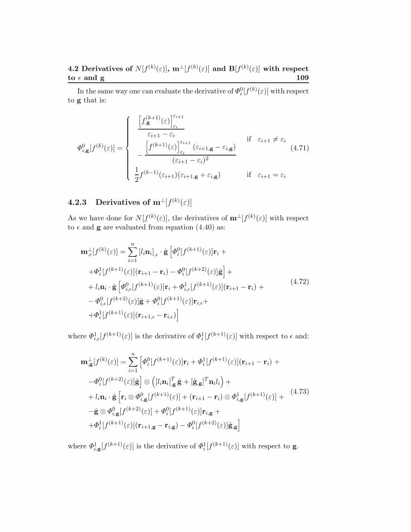
4.2 Derivatives of N [f (k)(ε)], m⊥[f (k)(ε)] and B[f (k)(ε)] with respectto ε and g 109
In the same way one can evaluate the derivative of Φ0i [f
(k)(ε)] with respectto g that is:
Φ0i,g [f (k)(ε)] =
[f
(k+1),g (ε)
]εi+1
εi
εi+1 − εi
−
[f (k+1)(ε)
]εi+1
εi
(εi+1,g − εi,g)
(εi+1 − εi)2
if εi+1 6= εi
12f (k−1)(εi+1)(εi+1,g + εi,g) if εi+1 = εi
(4.71)
4.2.3 Derivatives of m⊥[f (k)(ε)]
As we have done for N [f (k)(ε)], the derivatives of m⊥[f (k)(ε)] with respectto ε and g are evaluated from equation (4.40) as:
m⊥,ε [f
(k)(ε)] =n∑
i=1
[lini],ε · g[Φ0
i [f(k+1)(ε)]ri +
+Φ1i [f
(k+1)(ε)](ri+1 − ri) − Φ0i [f
(k+2)(ε)]g]+
+ lini · g[Φ0
i,ε[f(k+1)(ε)]ri + Φ1
i,ε[f(k+1)(ε)](ri+1 − ri) +
− Φ0i,ε[f
(k+2)(ε)]g + Φ0i [f
(k+1)(ε)]ri,ε+
+Φ1i [f
(k+1)(ε)](ri+1,ε − ri,ε)]
(4.72)
where Φ1i,ε[f
(k+1)(ε)] is the derivative of Φ1i [f
(k+1)(ε)] with respect to ε and:
m⊥,g[f (k)(ε)] =
n∑
i=1
[Φ0
i [f(k+1)(ε)]ri + Φ1
i [f(k+1)(ε)](ri+1 − ri) +
−Φ0i [f
(k+2)(ε)]g]⊗([lini]
T,g g + [g,g]Tnili
)+
+ lini · g[ri ⊗ Φ0
i,g[f (k+1)(ε)] + (ri+1 − ri) ⊗ Φ1i,g[f (k+1)(ε)] +
−g ⊗ Φ0i,g[f (k+2)(ε)] + Φ0
i [f(k+1)(ε)]ri,g +
+Φ1i [f
(k+1)(ε)](ri+1,g − ri,g) − Φ0i [f
(k+2)(ε)]g,g
]
(4.73)
where Φ1i,g[f (k+1)(ε)] is the derivative of Φ1
i [f(k+1)(ε)] with respect to g.

110 Integration formulas for polygonal sections
The derivative of the functions Φ1i [f
(k)(ε)] with respect to ε is obtaineddifferentiating equation (4.39) as follows:
Φ1i,ε[f
(k)(ε)] =f
(k+1),ε (εi+1)εi+1 − εi
−
[f
(k+2),ε (ε)
]εi+1
εi
(εi+1 − εi)2+
−f(k+1)(εi+1)(εi+1,ε − εi,ε)
(εi+1 − εi)2+
+2
[f (k+2)(ε)
]εi+1
εi
(εi+1,ε − εi,ε)
(εi+1 − εi)3
(4.74)
In the cases in which εi+1 = εi the same strategy adopted for the evaluationof Φ0
i,ε[f(k)(ε)] is used after re-writing Φ1
i,ε[f(k)(ε)] in the form:
Φ1i,ε[f
(k)(ε)] =1
(εi+1 − εi)3
f (k+1),ε (εi+1)(εi+1 − εi)2+
−[f (k+2),ε (ε)
]εi+1
εi
(εi+1 − εi)+
−f (k+1)(εi+1)(εi+1,ε − εi,ε)(εi+1 − εi)+
+2[f (k+2)(ε)
]εi+1
εi
(εi+1,ε − εi,ε)
(4.75)
The relevant limit for εi+1 → εi is in the form 0/0. L’Hopital’s rule is, thus,applied as follows:
limεi+1→εi
Φ1i,ε[f
(k)(ε)] =
= limεi+1→εi
13(εi+1 − εi)2
f (k+1),ε (εi+1)(εi+1 − εi)+
+f (k),ε (εi+1)(εi+1 − εi)2 −
[f (k+2),ε (ε)
]εi+1
εi
+
−f (k)(εi+1)(εi+1,ε − εi,ε)(εi+1 − εi)+
+f (k+1)(εi+1)(εi+1,ε − εi,ε)
(4.76)

4.2 Derivatives of N [f (k)(ε)], m⊥[f (k)(ε)] and B[f (k)(ε)] with respectto ε and g 111
which is still in the form 0/0. L’Hopital’s rule is applied again yielding:
limεi+1→εi
Φ1i,ε[f
(k)(ε)] =
= limεi+1→εi
16(εi+1 − εi)
3f (k)
,ε (εi+1)(εi+1 − εi)+
+f (k−1),ε (εi+1)(εi+1 − εi)2+
−f (k−1)(εi+1)(εi+1,ε − εi,ε)(εi+1 − εi)
=
=16f (k−1)(εi+1) (2εi+1,ε + εi,ε)
(4.77)
where use of (4.53) has been made.Thus we extend the function Φ1
i,ε[f(k)(ε)] to the cases where εi+1 = εi as:
Φ1i,ε[f
(k)(ε)] =
f(k+1),ε (εi+1)εi+1 − εi
−
[f
(k+2),ε (ε)
]εi+1
εi
(εi+1 − εi)2+
−f(k+1)(εi+1)(εi+1,ε − εi,ε)
(εi+1 − εi)2+
+2
[f (k+2)(ε)
]εi+1
εi
(εi+1,ε − εi,ε)
(εi+1 − εi)3
if εi+1 6= εi
16f (k−1)(εi+1) (2εi+1,ε + εi,ε) if εi+1 = εi
(4.78)
Similarly the derivative of Φ1i [f
(k)(ε)] with respect to g is equal to:
Φ1i,g [f (k)(ε)] =
f(k+1),g (εi+1)εi+1 − εi
−
[f
(k+2),g (ε)
]εi+1
εi
(εi+1 − εi)2+
−f(k+1)(εi+1)(εi+1,g − εi,g)
(εi+1 − εi)2+
+2
[f (k+2)(ε)
]εi+1
εi
(εi+1,g − εi,g)
(εi+1 − εi)3
if εi+1 6= εi
16f (k−1)(εi+1) (2εi+1,g + εi,g) if εi+1 = εi
(4.79)

112 Integration formulas for polygonal sections
4.2.4 Derivatives of B[f (k)(ε)]
The derivative of B[f (k)(ε)] with respect to ε is evaluated differentiatingequation (4.50):
B,ε[f (k)(ε)] =n∑
i=1
([lini],ε · g)Ai + (lini · g)Ai,ε (4.80)
where the tensor:
Ai = Φ0i [f
(k+1)(ε)](ri ⊗ ri)+
+Φ1i [f
(k+1)(ε)][ri ⊗ (ri+1 − ri) + (ri+1 − ri) ⊗ ri]+
+Φ2i [f
(k+1)(ε)][(ri+1 − ri) ⊗ (ri+1 − ri)]+
−Φ0i [f
(k+2)(ε)][ri ⊗ g + g ⊗ ri]+
−Φ1i [f
(k+2)(ε)][(ri+1 − ri) ⊗ g + g ⊗ (ri+1 − ri)]+
+2Φ0i [f
(k+3)(ε)](g⊗ g)
(4.81)
has been introduced. Differentiating the previous formula one gets:
Ai,ε = Φ0i,ε[f
(k+1)(ε)](ri ⊗ ri)+
+Φ0i [f
(k+1)(ε)](ri,ε ⊗ ri + ri ⊗ ri,ε)+
+Φ1i,ε[f
(k+1)(ε)][ri ⊗ (ri+1 − ri) + (ri+1 − ri)⊗ ri]+
+Φ1i [f
(k+1)(ε)][ri,ε ⊗ (ri+1 − ri) + ri ⊗ (ri+1,ε − ri,ε)+
+(ri+1,ε − ri,ε) ⊗ ri + (ri+1 − ri) ⊗ ri,ε]+
+Φ2i,ε[f
(k+1)(ε)][(ri+1 − ri)⊗ (ri+1 − ri)]+
+Φ2i [f
(k+1)(ε)][(ri+1,ε − ri,ε) ⊗ (ri+1 − ri)+
+(ri+1 − ri) ⊗ (ri+1,ε − ri,ε)]+
−Φ0i,ε[f
(k+2)(ε)][ri ⊗ g + g ⊗ ri]+
−Φ0i [f
(k+2)(ε)][ri,ε ⊗ g + g ⊗ ri,ε]+
−Φ1i,ε[f
(k+2)(ε)][(ri+1 − ri)⊗ g + g ⊗ (ri+1 − ri)]+
−Φ1i [f
(k+2)(ε)][(ri+1,ε − ri,ε) ⊗ g + g ⊗ (ri+1,ε − ri,ε)]+
+2Φ0i,ε[f
(k+3)(ε)](g⊗ g)
(4.82)
The derivatives of Φ0i [f
(k)(ε)] and Φ1i [f
(k)(ε)] with respect to ε are given byequations (4.70) and (4.78), respectively. In the same way Φ2
i,ε[f(k)(ε)] is

4.2 Derivatives of N [f (k)(ε)], m⊥[f (k)(ε)] and B[f (k)(ε)] with respectto ε and g 113
obtained differentiating equation (4.49):
Φ2i,ε[f
(k)(ε)] =f
(k+1),ε (εi+1)εi+1 − εi
− f (k+1)(εi+1)(εi+1,ε − εi,ε)(εi+1 − εi)2
+
−2f
(k+2),ε (εi+1)
(εi+1 − εi)2+ 4
f (k+2)(εi+1)(εi+1,ε − εi,ε)(εi+1 − εi)3
+
+2
[f
(k+3),ε (ε)
]εi+1
εi
(εi+1 − εi)3− 6
[f (k+3)(ε)
]εi+1
εi
(εi+1,ε − εi,ε)
(εi+1 − εi)4
(4.83)
The same strategy adopted for evaluating Φ0i,ε[f
(k)(ε)] and Φ1i,ε[f
(k)(ε)] in thecases in which εi+1 = εi is used here. To this end we re-write the previousformula as:
Φ2i,ε[f
(k)(ε)] =1
(εi+1 − εi)4
f (k+1),ε (εi+1)(εi+1 − εi)3+
−f (k+1)(εi+1)(εi+1,ε − εi,ε)(εi+1 − εi)2+
−2f (k+2),ε (εi+1)(εi+1 − εi)2
+4f (k+2)(εi+1)(εi+1,ε − εi,ε)(εi+1 − εi)+
+2[f (k+3),ε (ε)
]εi+1
εi
(εi+1 − εi)+
−6[f (k+3)(ε)
]εi+1
εi
(εi+1,ε − εi,ε)
(4.84)
whose limit for εi+1 → εi is in the form 0/0. Application of L’Hopital’s ruleyields:
limεi+1→εi
Φ2i,ε[f
(k)(ε)] = limεi+1→εi
14(εi+1 − εi)3
f (k),ε (εi+1)(εi+1 − εi)3 + f (k+1)
,ε (εi+1)(εi+1 − εi)2+
−f (k)(εi+1)(εi+1,ε − εi,ε)(εi+1 − εi)2+
−2f (k+2),ε (εi+1)(εi+1 − εi)+
+2f (k+1)(εi+1)(εi+1,ε − εi,ε)(εi+1 − εi)+
+2[f (k+3),ε (ε)
]εi+1
εi
− 2f (k+2)(εi+1)(εi+1,ε − εi,ε)
(4.85)

114 Integration formulas for polygonal sections
L’Hopital’s rule is applied again since the previous limit is again in the form0/0:
limεi+1→εi
Φ2i,ε[f
(k)(ε)] = limεi+1→εi
112(εi+1 − εi)2
f (k−1),ε (εi+1)(εi+1 − εi)3 + 4f (k)
,ε (εi+1)(εi+1 − εi)2+
−f (k−1)(εi+1)(εi+1,ε − εi,ε)(εi+1 − εi)2
(4.86)
Finally we extend the domain of the function Φ2i,ε[f
(k)(ε)] of equation (4.83)assuming the value
Φ2i,ε[f
(k)(ε)] =112f (k−1)(εi+1)(3εi+1,ε + εi,ε) (4.87)
for the cases in which εi+1 = εi.
Differentiating equation (4.50) with respect to g we get:
B,ε[f (k)(ε)] =n∑
i=1
Ai ⊗([lini]
T,g g + [g,g]Tnili
)+ (lini · g)Ai,g (4.88)

4.2 Derivatives of N [f (k)(ε)], m⊥[f (k)(ε)] and B[f (k)(ε)] with respectto ε and g 115
where the derivative of Ai with respect to g is obtained from equation (4.81):
Ai,g = (ri ⊗ ri)⊗ Φ0i,g[f (k+1)(ε)]+
+Φ0i [f
(k+1)(ε)][(ri,g ⊗ ri)T + ri ⊗ ri,g
]+
+[ri ⊗ (ri+1 − ri) + (ri+1 − ri)⊗ ri] ⊗ Φ1i,g[f (k+1)(ε)]+
+Φ1i [f
(k+1)(ε)][ri,g ⊗ (ri+1 − ri)]T + ri ⊗ (ri+1,g − ri,g)+
+[(ri+1,g − ri,g)⊗ ri]T + (ri+1 − ri) ⊗ ri,g
+
+[(ri+1 − ri)⊗ (ri+1 − ri)] ⊗ Φ2i,g[f (k+1)(ε)]+
+Φ2i [f
(k+1)(ε)][(ri+1,g − ri,g) ⊗ (ri+1 − ri)]T+
+(ri+1 − ri)⊗ (ri+1,g − ri,g)+
−[ri ⊗ g + g ⊗ ri]⊗ Φ0i,g[f (k+2)(ε)]+
−Φ0i [f
(k+2)(ε)][(ri,g ⊗ g)T + ri ⊗ g,g+
+(g,g ⊗ ri)T + g ⊗ ri,ε
]+
−[(ri+1 − ri)⊗ g + g ⊗ (ri+1 − ri)] ⊗ Φ1i,g[f (k+2)(ε)]+
−Φ1i [f
(k+2)(ε)][(ri+1,g − ri,g) ⊗ g]T + (ri+1 − ri) ⊗ g,g+
+[g,g ⊗ (ri+1 − ri)]T + g ⊗ (ri+1,g − ri,g)+
+2(g ⊗ g) ⊗ Φ0i,g[f (k+3)(ε)]+
+2Φ0i [f
(k+3)(ε)][(g,g ⊗ g)T + g ⊗ g,g
]
(4.89)
where the third order tensors of the kind (a,g ⊗ b)T are expressed in indexnotation as:
[(a,g ⊗ b)T
]jkl
= (a,g ⊗ b)jlk = aj,lbk (4.90)
The quantities Φ0i,g[f (k)(ε)] and Φ1
i,g[f (k)(ε)] are given from the relevantequations in the previous two subsections. For what concerns the derivativeof Φ2
i [f(k)(ε)] with respect to g the same strategy adopted for Φ2
i,ε[f(k)(ε)]
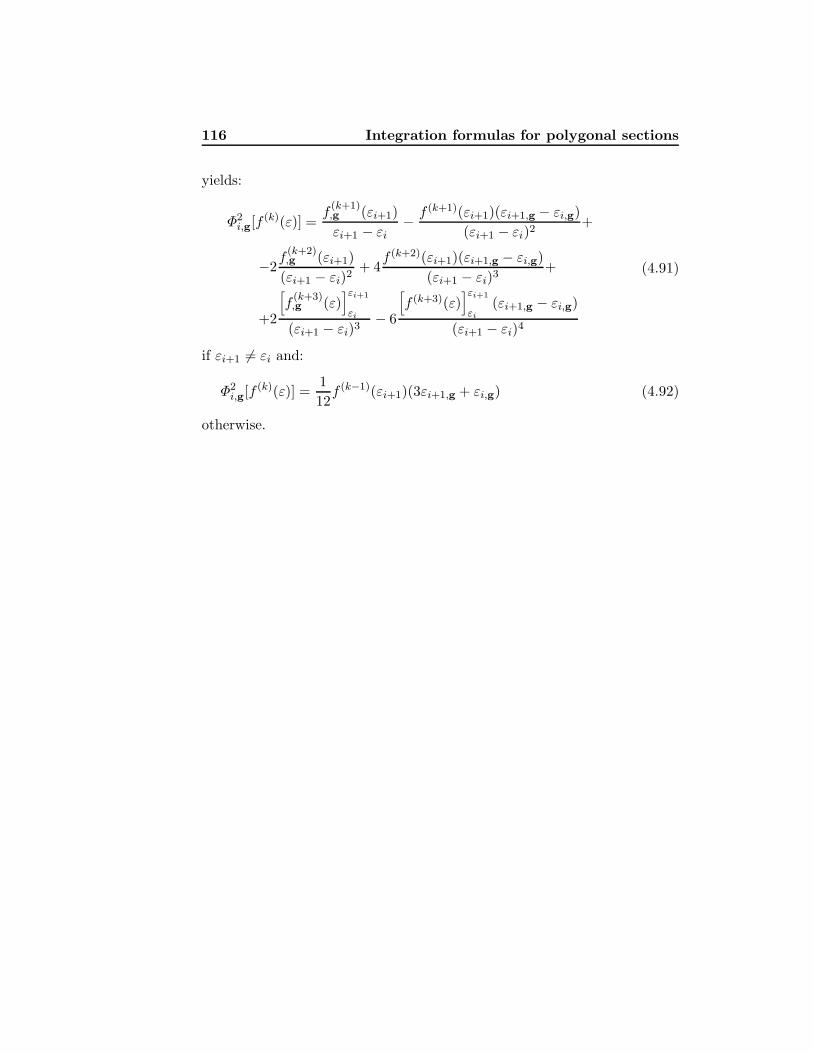
116 Integration formulas for polygonal sections
yields:
Φ2i,g[f (k)(ε)] =
f(k+1),g (εi+1)εi+1 − εi
− f (k+1)(εi+1)(εi+1,g − εi,g)(εi+1 − εi)2
+
−2f
(k+2),g (εi+1)
(εi+1 − εi)2+ 4
f (k+2)(εi+1)(εi+1,g − εi,g)(εi+1 − εi)3
+
+2
[f
(k+3),g (ε)
]εi+1
εi
(εi+1 − εi)3− 6
[f (k+3)(ε)
]εi+1
εi
(εi+1,g − εi,g)
(εi+1 − εi)4
(4.91)
if εi+1 6= εi and:
Φ2i,g[f (k)(ε)] =
112f (k−1)(εi+1)(3εi+1,g + εi,g) (4.92)
otherwise.

Chapter 5
Inelastic stress-strain laws
The integration formulas developed in chapter 4 can be used for non-linearelastic stress-strain relations, i.e. when the plastic strain distribution onthe section is neglected. In this chapter we will show how to adapt suchformulas to the case of more complex material models which account for thedeformation hystory of each point of the section.
Stress-strain relations commonly used for the points P of a non-linear RCsection is similar to the one shown in figure 5.1.
Figure 5.1: Plastic non-linear stress-strain relation
It is characterized by a non-linear envelope curve (OABC) which corre-sponds to an uniaxial monotonic loading of P. Unloading-reloading paths(BDO) are given as a function of the strain εm which is the maximum com-pressive value that the axial strain has ever reached at P. In general thecomplete unloading strain εp, corresponding to the residual or plastic strainin P, has a value which is given as a non-linear function of εm:
εp = εp(εm) (5.1)

118 Inelastic stress-strain laws
Clearly, once the value of εm is assigned, the behavior of P is univocallydetermined as a function of the current strain ε:
σ(r) = σ[εm(r), ε(r)] (5.2)
where r is the position vector of the generic point P.Since εm is responsible for the behavior of the points of the section, a
partition of the section can be executed by grouping the points where oneof the previous states of the section produces maximum values of the strain.
Let us consider, for instance, the case shown in figure 5.2, and imaginethat a sequence of three strain parameter vectors d1, d2 and d3, whichcorrespond to strain states of the section previous then the current one, aregiven. By comparing the values of such vectors the partitions P1 and P3,shown in figure 5.2, are determined.
Figure 5.2: Partition of the section according to the previously attainedmaximum strain
In particular, P1 is the portion of the section where the maximum strainis attained when d1 acts on the section. The maximum strain on P1 is, thus,given by:
εm1 = ε1 + g1 · r with dT1 = ε1, gx1, gy1 (5.3)
Similarly P3 is the partition where d3 maximizes the strain:
εm3 = ε3 + g3 · r with dT3 = ε3, gx3, gy3 (5.4)
Conversely, d2 does not maximize the strain at any point of the section,thus there is no partition related to it.

119
Since the values of the maximum strain are given for each partition, thestress-strain law is determined with a unique non-linear expression which isa function of the current strain ε, as shown in figure 5.3, where the case ofthe partition P3 is considered.
Figure 5.3: Stresses on partition P3
The maximum strain εm3 is given, thus the value of the plastic strain εp3
is evaluated by means of the relation εp = εp(εm). If, at the generic pointP, the current strain ε attains values greater than the ones given by εm3 thestress at P will follow the envelope curve of the material stress-strain law.Such behaviour is shown by the curve AB in figure 5.3.
Similarly, the strain is decreasing at the points of the section where εp3 <ε < εm3 thus the stress is evaluated according to the unloading-reloadingbehaviour of the material. The curve BC in figure 5.3 shows such behaviour.
Finally, the points where ε < εp3 are completely unloaded and the stressis null as shown in figure 5.3 between the points C and D.
Since each of the paths AB, BC and CD is determined by means ofa unique expression containing the value attained by εm3, εp3 and ε, theintegration formulas described in chapter 4 can be applied for the evaluationof the force vector and the stiffness matrix of a section in which the materialmodel of figure 5.1 is considered.
To fix yhe ideas the application of the procedure above will be illustratedin the following sections for a general class of non-linear stress-strain lawswhich can be set in the form:
σ(ε, εm) = εh(εm) + k(εm) + l(ε) (5.5)
Significant examples belonging to this class are a bilinear stress-strain lawwith no-tensile strenght, see section 5.3, and the Mander’s envelope curvediscussed in section 5.4.

120 Inelastic stress-strain laws
The case of a single partition will be considered, thus the maximum strainεm is given by:
εm(r) = εm + gm · r (5.6)
the plastic strain is evaluated as a function of εm:
εp(r) = εp[εm(r)] (5.7)
and the current strain is evaluated as:
ε(r) = ε+ g · r (5.8)
5.1 Partition of the section
The partition of the section is a procedure which we refer to in order todivide polygonal sections. Hereafter we are going to illustrate how the co-ordinates of the vertices of the partitions are determined and how theirderivatives with respect to the strain parameters ε and g are evaluated.
We remind that a Cartesian co-ordinate system with origin O and axesx and y lying on the plane of the cross section is introduced. The pointsof the plane x − y are identified by means of the relevant position vectorr = (x, y)T . One or more polygonal domains Ω are defined by means oftheir vertices ri ordered counter-clockwise as shown in figure 5.4.
Figure 5.4: Polygonal section
A strain field ε(r) is defined on the polygonal domain such that:
ε(r) = ε+ g · r (5.9)

5.1 Partition of the section 121
Also one or two auxiliary strain fields εa(r) with a = 1, 2 are defined onthe polygons and are evaluated as:
εa(r) = εa + ga · r (5.10)
The problem we want solve here is that of evaluating the vertices of asub-domain Ωp of the polygon Ω according to definitions of the kind:
Ωp1 = r ∈ Ω : ε1(r) ≤ ε(r) (5.11)
Ωp2 = r ∈ Ω : ε(r) ≤ ε2(r) (5.12)
or:
Ωp3 = r ∈ Ω : ε1(r) ≤ ε(r) ≤ ε2(r) (5.13)
Three possible partitions Ωp1, Ωp2 and Ωp3 are shown in figure 5.5.
Figure 5.5: Example of three partitions
Let us consider, for instance, the case of equation (5.11), so that thevertices of the partition Ωp1 need to be determined. As it can be seen inthe figure, the vertices of each partition always pertain to the sides of theoriginal section Ω; thus a loop over each side of the section is executed.
At the generic loop the i-th side, i.e. the one with endpoints ri and ri+1,is considered. Clearly, the vertex ri of Ω is also a vertex of the partitionΩp1 if ε1(ri) ≤ ε(ri).

122 Inelastic stress-strain laws
Since the components of ri do not depend upon ε and g the followingrelations hold:
∂ri
∂ε= 0 ;
∂ri
∂g= 0 (5.14)
At the successive loop step the i+ 1-st side, i.e. the one with endpointsri+1 and ri+2, is considered. Consequently, in the procedure described above,the vertices ri+1 and ri+2 will take the place of the vertices ri and ri+1,respectively. The inequality ε1(ri+1) ≤ ε(ri+1), which has to be checked inorder to include ri+1 between the vertces of Ωp1, will be taken into accountonly at the loop step relevant to the i+ 1-st side.
Also another vertex of Ωp1 might lie on the side ri − ri+1, as shown infigure 5.6. Such a new vertex, namely rc, is associated with the intersection
Figure 5.6: Vertex rc on the i-th side.
between ε(r) and ε1(r). Its co-ordinates are evaluated by means of theprocedure described hereafter.
The segment which connects the points ri and ri+1, i.e. the i-th side ofthe section, is described by means of a parametric function:
r(ϑ) = ri + ϑ(ri+1 − ri) (5.15)
with 0 ≤ ϑ ≤ 1.The composition of ε(r) and ε1(r) with r(ϑ) yields:
ε[r(ϑ)] = ε(ri) + ϑ[ε(ri+1) − ε(ri)] (5.16)
and
ε1[r(ϑ)] = ε1(ri) + ϑ[ε1(ri+1) − ε1(ri)] (5.17)
The value of ϑ corresponding to the position of rc is evaluated by settingε[r(ϑ)] = ε1[r(ϑ)] which yields:
ϑc =ε1(ri) − ε(ri)
ε1(ri) − ε1(ri+1) + ε(ri+1)− ε(ri)(5.18)

5.1 Partition of the section 123
thus, rc is a vertex of the partition only if 0 < ϑc < 1. It is worth beingnoticed that if the denominator of formula (5.18) tends to zero, ϑc goes toinfinity and rc is not a vertex of the partition.
Conversely, in the case 0 < ϑc < 1 is satisfied, the components of rc areevaluated by means of formula (5.15):
rc = ri + ϑc(ri+1 − ri) (5.19)
The derivatives of rc with respect to ε and g are evaluated by differenti-ating equation (5.19):
∂rc
∂ε= (ri+1 − ri)
∂ϑc
∂ε;
∂rc
∂g= (ri+1 − ri)
∂ϑc
∂g(5.20)
where ∂ϑc/∂ε and ∂ϑc/∂g are evaluated by differentiating equation (5.18).Since the strain field ε1(r) does not depend upon the strain parameters
of ε(r) it turns out to be:
∂ε1(ri)∂ε
=∂ε1(ri+1)
∂ε= 0 (5.21)
and
∂ε1(ri)∂g
=∂ε1(ri+1)
∂g= 0 (5.22)
Conversely, as we have shown in section 4.2 and making use of formulas(5.14):
∂ε(ri)∂ε
=∂ε(ri+1)∂ε
= 1 (5.23)
and
∂ε(ri)∂g
= ri ;∂ε(ri+1)∂g
= ri+1 (5.24)
Thus, differentiating equation (5.18) we get:
∂ϑc
∂ε= − 1
ε1(ri) − ε1(ri+1) + ε(ri+1) − ε(ri)(5.25)
and
∂ϑc
∂g=
[ε1(ri+1) − ε(ri+1)]ri − [ε1(ri) − ε(ri)]ri+1
ε1(ri)− ε1(ri+1) + ε(ri+1) − ε(ri)(5.26)
After the components of rc and its derivatives have been determined thenext side of Ω is analyzed. Such new side is the one between ri+1 and ri+2.

124 Inelastic stress-strain laws
These two endpoints will take the place of ri and ri+1, respectively, in theprocedure described above.
Finally we remark that for the determination of a partition of the kind ofΩp2, i.e. when the inequality ε(r) ≤ ε2(r) is considered, we adopt the sameprocedure described above. The only difference is that, in order to includeri between the vertices of the partition, one has to check ε2(ri) ≥ ε(ri) inplace of ε1(ri) ≤ ε(ri).
Finally, partitions of the kind of Ωp3 can be obtained by means of anintersection between the partitionsΩp1 and Ωp2, since the following relationshold:
Ωp3 = r ∈ Ω : ε1(r) ≤ ε(r) ≤ ε2(r) =
= r ∈ Ωp1 : ε(r) ≤ ε2(r) =
= r ∈ Ωp2 : ε1(r) ≤ ε(r)(5.27)
Consequently, Ωp3 can be obtained applying twice the procedure describedabove.
5.2 Integration of inelastic stress-strain laws andrelevant derivatives
Let us consider stress-strain relations which are expressed in the form:
σ(ε, εm) = εh(εm) + k(εm) + l(ε) (5.28)
where the functions h(εm), k(εm) and l(ε) are determined according to theconsidered material model.
The strains ε and εm are expressed by means of the following linearfunctions:
ε(r) = ε+ g · r ; εm(r) = εm + gm · r (5.29)
where r is the vector containing the coordinates of the points of the sectionΩ in the considered reference system.
Substitution of ε(r) in (5.28) yields:
σ(ε, εm) = εh(εm) + h(εm)g · r + k(εm) + l(ε) (5.30)
With reference to the function σ(ε, εm) of the last equation, the followingintegrals need to be evaluated:
N [σ(ε, εm)] =∫
Ωσ(ε, εm)dΩ ; m⊥[σ(ε, εm)] =
∫
Ωσ(ε, εm)rdΩ (5.31)

5.2 Integration of inelastic stress-strain laws and relevantderivatives 125
Substituting (5.30) in the first integral above one gets:
N [σ(ε, εm)] = ε
∫
Ωh(εm)dΩ + g ·
[ ∫
Ωh(εm)rdΩ
]+∫
Ωk(εm)dΩ+
+∫
Ωl(ε)dΩ =
= εN [h(εm)] + g ·m⊥[h(εm)] +N [k(εm)] +N [l(ε)]
(5.32)
where the relevant formulas of section 4.1 are used.Differentiation of equation (5.32) with respect to ε yields:
N,ε[σ(ε, εm)] = N [h(εm)] + εN,ε[h(εm)] + g ·m⊥,ε [h(εm)]+
+N,ε[k(εm)] +N,ε[l(ε)](5.33)
where the derivatives N,ε[h(εm)], m⊥,ε [h(εm)] and N,ε[k(εm)] are evaluated
by means of the same formulas used for N,ε[l(ε)], reported in section 4.2, inwhich one has to account for the fact that εm is independent of ε.
Similarly the derivative of N [σ(ε, εm)] with respect to g is:
N,g[σ(ε, εm)] = εN,g[h(εm)] + m⊥[h(εm)] + m⊥,g[h(εm)]Tg+
+N,g[k(εm)] +N,g[l(ε)](5.34)
in which the formulas reported in sections 4.1 and 4.2 are again used withthe proviso that εm is not related to g.
Substitution of (5.30) in (5.31)2 yields:
m⊥[σ(ε, εm)] = ε
∫
Ωh(εm)rdΩ +
[∫
Ωh(εm)(r⊗ r)dΩ
]g+
+∫
Ωk(εm)rdΩ +
∫
Ωl(ε)rdΩ =
= εm⊥[h(εm)] + B[h(εm)]g + m⊥[k(εm)] + m⊥[l(ε)]
(5.35)
The derivative of m⊥[σ(ε, εm)] with respect to ε yields:
m⊥,ε [σ(ε, εm)] = m⊥[h(εm)] + εm⊥
,ε [h(εm)] + B,ε[h(εm)]g+
+m⊥,ε [k(εm)] + m⊥
,ε [l(ε)](5.36)
Finally differentiating equation (5.35) with respect to g one gets:
m⊥,g[σ(ε, εm)] = εm⊥
,g[h(εm)] + B[h(εm)] + B,g[h(εm)]Tg+
+m⊥,g[k(εm)] + m⊥
,g[l(ε)](5.37)

126 Inelastic stress-strain laws
where the third order tensor (B,g)T is expressed in index notation as:[(B,g)T
]jlk
= (B,g)jkl = Bjk,l (5.38)
Again, in equations (5.35), (5.36) and (5.37) the relevant formulas in sec-tions 4.1 and 4.2 are used and, when appropriate, the independence betweenεm and the two parameters ε and g has to be taken into account.
5.3 Inelastic bilinear stress-strain law with no ten-sile strength
Let us consider the case of the material model described in Figure 5.7 withthe assumption that compressive stresses and strains are positive. The en-velope curve OABC is bilinear. Once the strain reaches its maximum com-pressive value, i.e. point B, an unloading will follow the path BD. Furtherunloading will not produce any stress increment since the material does nothave any tensile strength. Finally successive reloading is assumed to takeplace along the curve ODBC.
Figure 5.7: bilinear material model with no tension strength
The envelope curve (OABC) has the following analytical expression:
e(ε) =
0 if ε ≤ 0Eeε if 0 ≤ ε ≤ εy(Ee −Eh)εy +Ehε if εy ≤ ε
(5.39)
where εy is the yielding strain. The elastic stiffness is Ee and the hardeningis Eh.
When the strain ε reaches values beyond the yielding strain εy , up to themaximum compressive strain εm, a plastic strain εp is produced. Accord-ingly, there will be a part of the section, namely Ω1, where the maximum

5.3 Inelastic bilinear stress-strain law with no tensile strength127
compressive strain has never reached values beyond the yielding strain incompression, and where no plastic strain has been ever produced. Con-versely, on the remaining part of the section, i.e. Ω2, the maximum com-pressive strain is εm ≥ εy , hence the value of εp is not null on Ω2 as promptsfrom the next formula:
εp[εm(r)] =
0 on Ω1
[εm(r)− εy ]
(1 − Eh
Ee
)on Ω2
(5.40)
The two sub domains Ω1 and Ω2 are determined by means of the proceduredescribed in the section 5.1 with the strain limits reported in the followingequation:
Ω =
Ω1 = r ∈ Ω : εm(r) ≤ εyΩ2 = r ∈ Ω : εy ≤ εm(r)
(5.41)
Notice that the vertices of such partitions do not depend upon the currentstrain ε, so that their derivatives with respect to ε and g are zero.
While εp is null on Ω1, the plastic strain εp is a linear function of r whenr ∈ Ω2:
εp = εp + gp · r (5.42)
the strain parameters εp and gp are determined from (5.40)2 as:
εp = (εm − εy)
(1 − Eh
Ee
)gp = gm
(1− Eh
Ee
)(5.43)
Clearly, since the plastic strain is null on Ω1, the points of such partitionhave a behavior that follows the envelope curve e(ε):
σ1(ε, εm) = e(ε) (5.44)
Conversely, the stress at a point of the partition Ω2 is a function of thevalues attained by ε, εm and εp:
σ(ε, εm) =
0 on Ω2a
e(εm)εm − εp(εm)
[ε− εp(εm)] on Ω2b
e(ε) on Ω2c
(5.45)

128 Inelastic stress-strain laws
where e(εm) is given by equation (5.39) with εm used in place of ε. A furtherpartition of the domain Ω2 has been introduced as follows:
Ω2 =
Ω2a = r ∈ Ω2 : ε(r) ≤ εp[εm(r)]Ω2b = r ∈ Ω2 : εp[εm(r)] ≤ ε(r) ≤ εm(r)Ω2c = r ∈ Ω2 : εm(r) ≤ ε(r)
(5.46)
5.3.1 Determination of the functions h(εm), k(εm) and l(ε)
The goal of this section is that of re-writing the stress-strain law describedabove by means of a unique expression of the kind of equation (5.28) so asto make it integrable by means of the formulas of section 5.2.
On the partition Ω1 the stress-strain relation is coincident with the en-velope curve, so that the functions h(εm) and k(εm) of equation (5.28) haveto assume a null value while l(ε) = e(ε).
The stress-strain law is identically null on Ω2a; thus, on such domain, thefunctions h(εm), k(εm) and l(ε) are null too.
Substitution of (5.40)2 in (5.86)2 yields the stress-strain relation on Ω2b,that is:
σ2b(ε, εm) =e(εm)
εm − (εm − εy)
(1 − Eh
Ee
)[ε− (εm − εy)
(1 − Eh
Ee
)]=
=Eee(εm)ε
Eh(εm − εy) +Eeεy+
(Eh − Ee)(εm − εy)e(εm)Eh(εm − εy) + Eeεy
=
= εh2b(εm) + k2b(εm)
(5.47)
Finally the stress-strain law on Ω2c does not depend upon εp and εm;hence, the functions h(εm) and k(εm) assume null values on such domains.Conversely the function l(ε) is equal to the envelope curve on Ω2c and isnull everywhere else.
As a result we can write the stress strain relation on Ω as:
σ(ε, εm) = εh(εm) + k(εm) + l(ε) (5.48)
where:
h(εm) =
0 on Ω1, Ω2a and Ω2c
Eee(εm)Eh(εm − εy) +Eeεy
on Ω2b
(5.49)

5.3 Inelastic bilinear stress-strain law with no tensile strength129
k(εm) =
0 on Ω1, Ω2a and Ω2c
(Eh − Ee)(εm − εy)e(εm)Eh(εm − εy) + Eeεy
on Ω2b
(5.50)
and:
l(ε) =
0 on Ω2a and Ω2b
e(ε) on Ω1 and Ω2c
(5.51)
Primitives of h(εm) and its derivative
The primitives of the function h(εm), up to the fourth order, and its firstderivative are used in chapter 4 and in section 5.2 in order to evaluate thestress resultants and their derivatives. Hereafter we are going to furnish anexpression of such functions over each of the partitions considered in thesection 5.3.
As shown in section 5.3.1 the function h(εm) assumes a null value on thedomains Ω1, Ω2a and Ω2c; hence the primitives of h(εm) and its derivativeare identically null in such domains.
The expression of h(εm) on Ω2b is obtained from equation (5.88). Sub-stitution of (5.39) in (5.88) yields:
h2b(εm) =Eee(εm)
Eh(εm − εy) +Eeεy=
=
0 if εm ≤ 0
E2eεm
Eh(εm − εy) + Eeεyif 0 ≤ εm ≤ εy
Ee if εy ≤ εm
(5.52)
For 0 ≤ εm ≤ εy the first order primitives of h2b(εm) up to the fourthorder are:
h(1)2b1
(εm) = −E2
e
[(Ee −Eh)εy log(Ehεm +Eeεy −Ehεy) −Ehεm
]
E2h
(5.53)
h(2)2b1
(εm) =−E2
e
2E3h
− Ehεm[Eh(εm − 2εy) + 2Eeεy ]+
+2(Ee −Eh)εy [Eh(εm − εy) +Eeεy ] log(Ehεm+
+Eeεy − Ehεy)
(5.54)

130 Inelastic stress-strain laws
h(3)2b1
(εm) =−E2
e
12E4h
− Ehεm[3EeEh(3εm − 4εy)εy + 6E2
eε2y+
+E2h(2ε2m − 9εmεy + 6ε2y)]+ 6(Ee −Eh)εy [Eh(εm − εy)+
+Eeεy ]2 log(Ehεm +Eeεy − Ehεy)
(5.55)
h(4)2b1
(εm) =E2
e
72E5h
3E4hε
4m − 22E3
h(Eh −Ee)ε3mεy+
+30(Ee − Eh)2E2hε
2mε
2y − 12Eh(Eh − Ee)3εmε3y+
−12(Ee − Eh)4ε4y log(Ehεm +Eeεy −Ehεy)+
+12Eh(Eh − Ee)εmεy [3EeEh(εm − 2εy)εy + 3E2eε
2y+
+E2h(ε2m − 3εmεy + 3ε2y)] log(Ehεm +Eeεy − Ehεy)
(5.56)
The primitives of h2b(εm) for εy ≤ εm are reported hereafter:
h(1)2b2
(εm) =Ee
E2h
Eh[Eh(εm − εy) + Eeεy ]+
+Ee(Eh −Ee)εy log(Eeεy)(5.57)
h(2)2b2
(εm) =Ee
2E3h
EeEh[E2h(εm − εy)2 +EeEh(2εm − 3εy)εy+
+2E2eε
2y ]− 2Ee(Ee − Eh)εy[Eh(εm − εy) + Eeεy ] log(Eeεy)
(5.58)
h(3)2b2
(εm) =Ee
12E4h
Eh[2E3h(εm − εy)3 + 3E2
eEh(4εm − 5εy)ε2y+
+6E3eε
3y +EeE
2hεy(6ε
2m − 18εmεy + 11ε2y)]+
−6Ee(Ee −Eh)εy [Eh(εm − εy) +Eeεy ]2 log(Eeεy)
(5.59)
h(4)2b2
(εm) =Ee
72E5h
Eh[3E4h(εm − εy)4 + 6E3
eEh(6εm − 7εy)ε3y+
+12E4eε
4y + 2E2
eE2hε
2y(18ε2m − 45εmεy + 26ε2y)+
+EeE3hεy(12ε3m − 54ε2mεy + 66εmε2y − 25ε3y)]+
−12Ee(Ee − Eh)εy[Eh(εm − εy) + Eeεy ]3 log(Eeεy)
(5.60)
The constants of integration of the primitives of h2b2(εm) have been eval-uated by solving the equations h(j)
2b2(εy) = h
(j)2b1
(εy) for j = 1, ..., 4.Also the derivative of h(εm) will be used in the integration formulas
described in the following sections. Notice that such derivative is used just

5.3 Inelastic bilinear stress-strain law with no tensile strength131
in the cases in which the strain field εm is constant thus h′(εm) = h(−1)(εm)is not needed to be continuous.
For 0 ≤ εm ≤ εy the derivative of h2b1(εm) is:
h(−1)2b1
(εm) =E2
e (Ee −Eh)εy[Eh(εm − εy) + Eeεy ]2
(5.61)
and, for εy ≤ εm, it is h(−1)2b2
(εm) = 0.
Primitives of k(εm) and its derivative
In the same way as it has been done for h(εm) we will evaluate the primitivesof k(εm) and its derivative only where k(εm) 6= 0, i.e. on Ω2b for 0 ≤ εm.In the other cases k(εm) is identically null, the constants of integration arenull too what makes its derivative and primitives vanish.
The expression of k(εm) on Ω2b is obtained from equation (5.88). Sub-stitution of (5.39) in (5.88) yields:
k2b(εm) =(Eh −Ee)(εm − εy)e(εm)Eh(εm − εy) +Eeεy
=
=
0 if εm ≤ 0
Ee(Eh −Ee)(εm − εy)εmEh(εm − εy) + Eeεy
if 0 ≤ εm ≤ εy
(Eh −Ee)(εm − εy) if εy ≤ εm
(5.62)
For 0 ≤ εm ≤ εy the primitives of k(εm) are:
k(1)2b1
(εm) =−Ee(Ee −Eh)
2E3h
[Ehεm(Ehεm − 2Eeεy)+
+2Ee(Ee −Eh)ε2y log(Ehεm + Eeεy −Ehεy)](5.63)
k(2)2b1
(εm) =−Ee(Ee −Eh)
6E4h
Ehεm[E2hε
2m − 6E2
eε2y+
+3EeEhεy(−εm + 2εy)] + 6Ee(Ee − Eh)ε2y [Eh(εm − εy)+
+Eeεy ] log(Ehεm + Eeεy −Ehεy)
(5.64)
k(3)2b1
(εm) =−Ee(Ee −Eh)
24E5h
Ehεm[E3hε
3m − 6E2
eEh(3εm − 4εy)ε2y+
−12E3eε
3y − 2EeE
2hεy(2ε
2m − 9εmεy + 6ε2y)]+
+12Ee(Ee −Eh)ε2y [Eh(εm − εy) +Eeεy ]2 log(Ehεm+
+Eeεy − Ehεy)
(5.65)

132 Inelastic stress-strain laws
while for εy ≤ εm the primitives of k(εm) are:
k(1)2b2
(εm) =−(Ee − Eh)
2E3h
Eh[E2h(εm − εy)2 − 2E2
eε2y +EeEhε
2y ]+
+2E2e (Ee −Eh)ε2y log(Eeεy)
(5.66)
k(2)2b2
(εm) =−(Ee − Eh)
6E4h
Eh[E3h(εm − εy)3+
+EeE2h(3εm − 2εy)ε2y − 6E3
eε3y + 3E2
eEhε2y(−2εm + 3εy)]+
+6E2e (Ee −Eh)ε2y[Eh(εm − εy) + Eeεy ] log(Eeεy)
(5.67)
k(3)2b2
(εm) =−(Ee − Eh)
24E5h
Eh[E4h(εm − εy)4+
−6E3eEh(4εm − 5εy)ε3y − 12E4
eε4y + EeE
3hε
2y(6ε
2m+
−8εmεy + 3ε2y) − 2E2eE
2hε
2y(6ε
2m − 18εmεy + 11ε2y)]+
+12E2e(Ee − Eh)ε2y[Eh(εm − εy) + Eeεy ]2 log(Eeεy)
(5.68)
in which the integration constants have been evaluated by adopting the samestrategy adopted for h(εm).
Finally, for 0 ≤ εm ≤ εy the derivative of k(εm) is:
k(−1)2b1
(εm) =Ee
[Eh(εm − εy) +Eeεy ]2[E2
h(εm − εy)2+
+E2eεy(−2εm + εy)− EeEh(ε2m − 4εmεy + 2ε2y)]
(5.69)
while for εy ≤ εm it is k(−1)2b2
(εm) = Eh −Ee.
Primitives of l(ε) and its derivative
In the same way as it has been done for h(εm) and k(εm) we will evaluatethe primitives of l(ε) and its derivatives only on Ω1 and Ω2c, for 0 ≤ ε,where l(ε) = e(ε). In the other cases l(ε) is identically null, the constantsof integration are null too so that its derivative and its primitives are zero.
For 0 ≤ ε ≤ εy the primitives of l(ε) are:
l(1)11
(ε) = l(1)2c1
(ε) =Eeε
2
2(5.70)
l(2)11
(ε) = l(2)2c1
(ε) =Eeε
3
6(5.71)

5.4 Inelastic stress strain law with Mander’s envelope curve 133
l(3)11
(ε) = l(2)2c1
(ε) =Eeε
4
24(5.72)
while for εy ≤ ε the primitives of l(ε) are:
l(1)12
(ε) = l(1)2c2
(ε) =Eh(ε− εy)
2 +Ee(2ε− εy)εy2
(5.73)
l(2)12
(ε) = l(2)2c2
(ε) =Eh(ε− εy)
3 +Eeεy(3ε2 − 3εεy + ε2y)6
(5.74)
l(3)12
(ε) = l(2)2c2
(ε) =Eh(ε− εy)
4 −Eeεy(−4ε3 + 6ε2εy − 4εε2y + ε3y)24
(5.75)
in which the integration constants have been evaluated in the same way asit has been done for h(εm) and k(εm).
Finally, for 0 ≤ ε ≤ εy the derivative of l(ε) is l(−1)11
(ε) = l(−1)2c1
(ε) = Ee,
while for εy ≤ ε it is l(−1)12
(ε) = l(−1)2c2
(ε) = Eh.
5.4 Inelastic stress strain law with Mander’s en-
velope curve
The material model shown in figure 5.8 is described in this section. Still theassumption of positive stresses and strains in compression has been done.The envelope curve OABC is the one described in [61] while for the plasticbehavior of the material simpler assumptions have been considered. Themaximum compressive strain is determined once the material reaches thepoint B and starts unloading. The unloading path will take place along thesegment BD. From the point D a further unloading will not produce anystress increment since the material has not any tensile strength. Finallysuccessive reloading is assumed to take place along the curve ODBC.
The envelope curve [61] is determined by means of the following formula:
e(ε) =
0 if ε ≤ 0r f ′cc
ε
εcc
r − 1 +(ε
εcc
)r if 0 ≤ ε ≤ εcu(5.76)
where f ′cc and εcc are the confined concrete strength and the relevant strain.They are determined as function of the unconfined concrete strength f ′co andthe relevant strain εco as:
f ′cc = f ′co + k1fl ; εcc = εco
(1 + k2
fl
f ′co
)(5.77)

134 Inelastic stress-strain laws
where k1 and k2 are two numerical coefficients determined as a function ofthe concrete mix and the lateral pressure fl due to the confinement. For adescription of how to determine the parameters k1 and k2 and the lateralpressure fl see [61].
The parameter r in (5.76) is also a function of the confinement and itsvalue is determined as:
r =Ec
Ec −Esec(5.78)
where Ec is the tangent stiffness of concrete:
Ec = 5000√f ′co MPa (5.79)
and Esec is the secant stiffness corresponding to the point of the envelopecurve where the material strength is reached:
Esec =f ′ccεcc
(5.80)
Finally εu is the ultimate concrete compression strain [61]. It is definedas the longitudinal strain at which the first fracture of the hoop occurs [86],since such strain can be regarded as the end of the region of the stress-strainlaw in which the confinement parameters are effective. Several approachesfor the determination of the value of εu are presented in literature. Here,we adopt a simple formula obtained by means of a simple manipulation ofthe formulas reported in [86] which well approximates the values obtainedwith more sophisticated methods:
εu = 0.004 + 0.9f ′cc − f ′co
300(5.81)
Figure 5.8: Inelastic material with Mander’s envelope curve

5.4 Inelastic stress strain law with Mander’s envelope curve 135
where f ′cc and f ′co are expressed in MPa.Since only positive values of εm will produce plastic strains we divide the
section in a part Ω1, where εm ≤ 0 and no plastic strain is produced, and apart Ω2, where εm ≥ 0 and εp is given by means of the following formula:
εp[εm(r)] =
0 on Ω1
εm − (εm + εa)e(εm)e(εm) + Ec εa
on Ω2
(5.82)
where
εa = a√εm εcc ; a =
εccεcc + εm
(5.83)
It is worth to notice that the value a = 0.09εm/εcc reported in [61] is notconsidered here since, for big values of εm, it gives an increasing stiffness ofthe unloading path. Such circumstance is in contrast with the assumptionof an increasing damage of the material.
The two sub domains Ω1 and Ω2 are determined by means of the proce-dure described in the section 5.1 with the strain limits reported hereafter:
Ω =
Ω1 = r ∈ Ω : εm(r) ≤ 0Ω2 = r ∈ Ω : 0 ≤ εm(r) ≤ εcu
(5.84)
Notice that the vertices of such partitions do not depend upon the currentstrain ε, thus their derivatives with respect to ε and g are null.
Since on Ω1 the plastic strain is null, the points of such partition have abehavior that follows the envelope curve e(ε):
σ1(ε, εm) = e(ε) (5.85)
Conversely, the stress in a point of the partition Ω2 is a function of thevalues attained by ε, εm and εp:
σ(ε, εm) =
0 on Ω2a
e(εm)εm − εp(εm)
[ε− εp(εm)] on Ω2b
e(ε) on Ω2c
(5.86)
where e(εm) is given by equation (5.76) with εm used in place of ε. A furtherpartition of the domain Ω2 has been introduced as follows:
Ω2 =
Ω2a = r ∈ Ω2 : ε(r) ≤ εp[εm(r)]Ω2b = r ∈ Ω2 : εp[εm(r)] ≤ ε(r) ≤ εm(r)Ω2c = r ∈ Ω2 : εm(r) ≤ ε(r)
(5.87)

136 Inelastic stress-strain laws
5.4.1 Determination of the functions h(εm), k(εm) and l(ε)
The goal of this section is that of re-writing the stress-strain law describedabove by means of a unique expression of the kind of equation (5.28) whichcan be integrated by means of the formulas of section 5.2.
On the partition Ω1 the stress-strain relation is coincident with the en-velope curve, thus h(εm) = 0 and k(εm) = 0 l(ε) = e(ε).
The stress-strain law is identically null on Ω2a, thus the functions h(εm),k(εm) and l(ε) assume a null value on such domain.
The stress-strain relation on Ω2b is given by equation (5.86)2, whichyields:
σ2ib(ε, εm) =e(εm)
εm − εp(εm)
[ε− εp(εm)
]=
=e(εm)
εm − εp(εm)ε − e(εm)
εm − εp(εm)εp(εm) =
= εh2ib(εm) + k2ib(εm)
(5.88)
Finally the stress-strain law on Ω2c does not depend upon εp and εm,thus the functions h(εm) and k(εm) are identically null on such domains.Conversely the function l(ε) is equal to the envelope curve.
As a result we can write the stress strain relation on Ω as:
σ(ε, εm) = εh(εm) + k(εm) + l(ε) (5.89)
with:
h(εm) =
0 on Ω1, Ω2a and Ω2c
e(εm)εm − εp(εm)
on Ω2b
(5.90)
k(εm) =
0 on Ω1, Ω2a and Ω2c
− e(εm)εm − εp(εm)
εp(εm) on Ω2b
(5.91)
and:
l(ε) =
0 on Ω2a and Ω2b
e(ε) on Ω1 and Ω2c
(5.92)

5.4 Inelastic stress strain law with Mander’s envelope curve 137
5.4.2 Considerations upon the partition of the section
A partition of the section involving a comparison between ε and εp is usedin equation (5.87) in order to distinguish between parts of the section whichare unloading and parts of the section where the stress is null.
Since εm corresponds to one of the previous states of the section it isa linear function of the position vector r. Conversely, εp is a non-linearfunction of εm, thus it is a non-linear function of r too. The partitions Ω2a
and Ω2b are determined by means of such non-linear relation which leads toobtain non-polygonal partitions, as shown in figure 5.9. Notwithstanding,we need all the partitions to be polygonal in order to adopt the formulas forevaluating the integrals over concrete sections.
Figure 5.9: Ω2a and Ω2b are non polygonal partitions
Polygonal approximations of the actual partitions are obtained by adopt-ing a fictitious strain εp = εp + gp · r which is determined by linearizing therelation εp(εm) for values of εm between εma and εmb:
εp(εm) = εp(εma) +εp(εmb) − εp(εma)
εmb − εma(εm − εma) (5.93)
The strain parameters of εp are determined as:
εp = εp(εma) +εp(εmb)− εp(εma)
εmb − εma(εm − εma)
gp =εp(εmb) − εp(εma)
εmb − εmagm
(5.94)
It is worth to notice that for εm < 0 we have εp = 0. Also for εm > εcuthe constitutive model is not defined. Consequently we need to approximatethe function εp(εm) only in the interval [0, εcu].

138 Inelastic stress-strain laws
Clearly any interpolation with a unique linear function will end up ina very rough approximation of εp(εm). Thus several intervals [εmai , εmbi ],matching the whole interval [0, εcu], are considered. In this way a piecewiselinear interpolation of εp(εm) is produced. Each of the intervals [εmai , εmbi ]corresponds to a partition of Ω2 defined as:
Ω2i = r ∈ Ω2 : εmai ≤ εm ≤ εmbi (5.95)
in which the relevant linear function εpi(εm) is defined.Each of the partitions Ω2i is further divided into two sub-partitions:Ω2ia = r ∈ Ω2i : ε ≤ εpi ≤ εΩ2ib = r ∈ Ω2i : εpi ≤ ε ≤ εm (5.96)
Since εpi(εm) is a linear approximation of εp(εm), onΩ2i , the sub-partitionsΩ2ia and Ω2ib approximate the non-polygonal partitions Ω2a and Ω2b, re-spectively, as shown in figure 5.10.
Figure 5.10: The sub-partitions Ω2ia and Ω2ib approximate the non-polygonal partitions Ω2a and Ω2b
Remind that Ω2c, obtained by means of(5.87)3, is still polygonal. Thusit does not need any special care.
5.4.3 Spline interpolation of h(εm), k(εm) and l(ε)
The very special form of the envelope curve e(ε) in (5.76) and the non-linear relation between εm and εp in (5.82) cause great difficulties in thedetermination of the primitives of the functions h(εm), k(εm) and l(ε) in

5.4 Inelastic stress strain law with Mander’s envelope curve 139
(5.90), (5.91) and (5.92), respectively. Here we furnish a spline interpolationof such functions so that they can be easily integrated over each partition.
Let us consider a continuous function f(x). We want to approximatef(x) by means of a third order polynomial:
p(x) = p0 + p1x+ p2x2 + p3x
3 (5.97)
for values of x between xa and xb. The four parameters p0, ... , p3 are thusdetermined by solving the following system of equations:
p(xa) = f(xa)
p(−1)(xa) = f (−1)(xa)
p(xb) = f(xb)
p(−1)(xb) = f (−1)(xb)
(5.98)
which is obtained by setting the value that f(x) and its derivative f (−1)(x)attain at the endpoints of the interval [xa, xb] equal to the value that p(x)and its derivative p(−1)(x) attain at the same points.
The system (5.98) is solved for the values of the four parameters p0, p1,p2 and p3 obtaining:
p0 =1
(xa − xb)3[f(xb)x3
a + xb(xb − xa)f (−1)(xb)x2a − 3xbf(xb)x2
a+
+x2b(xb − xa)f (−1)(xa)xa + 3x2
bf(xa)xa − x3bf(xa)]
(5.99)
p1 =1
(xa − xb)3xa(x2
a + xbxa − 2x2b)f
(−1)(xb)+
+6xb[f(xb) − f(xa)] − xb(xbxa − 2x2a + x2
b)f(−1)(xa)
(5.100)
p2 =1
(xa − xb)3(xbxa − 2x2
a + x2b)f
(−1)(xb)+
−(x2a + xbxa − 2x2
b)f(−1)(xa) + 3(xa + xb)[f(xa) − f(xb)]
(5.101)
p3 =(xa − xb)f (−1)(xa) + (xa − xb)f (−1)(xb) − 2f(xa) + 2f(xb)
(xa − xb)3(5.102)
It is worth to notice that we need to approximate h(εm), k(εm) and l(ε)in the interval [0, εcu] since they assume a null value elsewhere. Clearlyrepeating the previous steps for the three functions h(εm), k(εm) and l(ε)by assuming [xa, xb] = [0, εcu] will end up in a very rough approximation.

140 Inelastic stress-strain laws
For this reason we subdivide the whole interval [0, εcu] in several subintervals[xai , xbi] wherein the function is approximated with the relevant polynomialspi(x). They will form a piecewise polynomial, i.e. a spline interpolation ofthe actual function. Smaller the amplitude of the adjacent intervals [xai , xbi],finest the approximation of the actual function. Since the several intervalsrelevant to each polynomial segment of the spline function are adjacent, thefollowing property holds:
xai = xbi−1 (5.103)
meaning that the final endpoint of any interval is equal to the initial endpointof the successive one.
Primitives of h(εm), k(εm) and l(ε) and their derivatives
The functions h(εm), k(εm) and l(ε) are interpolated by means of splinesdefined in the interval [0, εcu]. Any single polynomial which compose thewhole spline function is a third order polynomial:
pi(x) = p0i + p1ix+ p2ix2 + p3ix
3 (5.104)
defined in the interval [xai, xbi ] ⊂ [0, εcu]. The variable x stands for εm ifthe spline refers to h(εm) or k(εm) and ε if it refers to l(ε).
The first order derivative of the generic polynomial pi(x) is:
p(−1)i (x) = p1i + 2p2ix+ 3p3ix
2 (5.105)
The first order primitive of the generic polynomial segment of the inter-polating spline is:
p(1)i (x) = p0ix+ p1i
x2
2+ p2i
x3
3+ p3i
x4
4+ P1i (5.106)
Since the primitive of the whole spline has to be continuous, the constantof integration P1i is determined by setting:
p(1)i (xai) = p
(1)i−1(xbi−1) ⇒ p
(1)i (xai) = p
(1)i−1(xai) (5.107)
where the property (5.103) has been used.Similarly the second, third and fourth order primitives of pi(x) are:
p(2)i (x) = p0i
x2
2+ p1i
x3
6+ p2i
x4
12+ p3i
x5
20+ P1ix+ P2i (5.108)
p(3)i (x) = p0i
x3
6+ p1i
x4
24+ p2i
x5
60+ p3i
x6
120+ P1i
x2
2+ P2ix+ P3i (5.109)

5.4 Inelastic stress strain law with Mander’s envelope curve 141
and
p(4)i (x) = p0i
x4
20+ p1i
x5
120+ p2i
x6
360+ p3i
x7
840+ P1i
x3
6+ P2i
x2
2+
+P3ix+ P4i
(5.110)
where P2i , P3i and P4i are determined by setting:
p(2)i (xai) = p
(2)i−1(xai) (5.111)
p(3)i (xai) = p
(3)i−1(xai) (5.112)
and
p(4)i (xai) = p
(4)i−1(xai) (5.113)
Let us consider the case of the polynomial defined in the interval withinitial endpoint xai = 0, which is equal to the initial endpoint of the inter-val [0, εcu] where the spline function is defined. This is the case in whichthe first polynomial segment of the spline function is considered. Thus thepolynomial pi−1(x) is not defined hence the constants of integration cannotbe determined by means of the procedure explained previously. Actually,recalling equations (5.90), (5.91) and (5.92), we have that the three func-tions h(εm), k(εm) and l(ε) assume a null value outside the interval [0, εcu].Thus we define pi−1(x) = 0 and we set equal to zero its primitives too. Con-sequently, all the constants of integration, relevant to the first polynomialsegment of the spline function, are null.

142 Inelastic stress-strain laws

Chapter 6
Numerical results
In order to show the effectiveness of the integration formulas presented inthis thesis, several numerical tests have been carried out by comparing theresults entailed by the proposed approach with those associated with theuse of fibers.
Specifically, two separate kind of tests have been conceived, one for thebilinear stress-strain law presented in section 5.3 and the other one for theMander’s constitutive law which, in a sense, is representative of complexstress-strain laws which either do not possess primitives amenable to anexact analytical form or are directly assigned as collection of experimentallydetermined pairs of stress-strain values.
In the former case, the fiber-free approach provides exact values bothfor the stress resultants, see e.g. integrals (5.32) and (5.35), and for itsderivatives, provided by formulas (5.33), (5.34), (5.36) and (5.37).
In the latter case, the constitutive law has to be somehow interpolatedso that the exact value of the stress resultants and of its derivatives permit-ted by the fiber-free approach pertains to the interpolated constitutive lawrather than to the original one.
In both cases aim of this section is to investigate on the degree of ap-proximation introduced by the adoption of the traditional fiber approach,to date the only existing method for integrating elastic-plastic normal stressfields.
6.1 Integration of bilinear stress-strain laws
It has been pointed out before that, in the case of bilinear stress-strain lawsthe fiber-free approach provides exact results both for the stress resultants

144 Numerical results
and its derivatives.However, in order to check the correctness of the formulas derived in the
previous sections and the relevant implementation, it has been decided tocompare the results obtained by the fiber-free approach with those associ-ated with the use of the traditional fiber approach. Due to the inherentapproximation of this last method an increasing number of fibers has beenconsidered up to a maximum allowed by the computer memory, on one side,and by the machine precision on the other.
As a representative example of the several numerical tests which havebeen carried out we discuss the results obtained for a rectangular section ofsize 0.3 × 0.4 made of the material described in section 5.3 with Ee = 10,Eh = 0.1 and εy = −1.
To provide this example, and the additional ones presented in the sequel,with a deeper engineering sense, we specify that, although unnecessary tomake the numerical tests consistent, the adopted units are meters for lengthsand Newton for forces.
The section has been analyzed by keeping constant ε = 0 and gy =0. A loading-unloading analysis has been executed by increasing the gx
component of the strain gradient from −0.5 to −10 and then decreasingback to −0.5 with steps of 0.5. The relevant My −gx curves obtained by thefiber-free approach and the fiber method is plotted in figure 6.1.
0 2 4 6 8 100.00
0.02
0.04
0.06
0.08
0.10
gx
My
Figure 6.1: My − gx relation
The force vector and the tangent matrix of the section relevant to the

6.1 Integration of bilinear stress-strain laws 145
last step of the analysis carried out by the fiber-free approach are:
N
Mx
My
=
−1.57978723404256E − 02
−1.08120190131281E − 03
−1.55366171317172E − 18
(6.1)
and
N,ε N,gx N,gy
Mx,ε Mx,gx Mx,gy
My,ε My,gx My,gy
=
6.31914893617021E − 01
3.32763693979175E − 02
1.19939865331208E − 18
3.32763693979176E − 02 −3.10461292091224E − 18
2.33642593644953E − 03 −1.25422987137241E − 18
−7.76446868316442E − 20 1.89574468085106E − 02
(6.2)
Notice that for computers with machine precision of 10−16, the values ofMy , N,gy , Mx,gy , My,ε and My,gx are numerically zero.
In this respect we remind that for a FORTRAN variable declared asreal*8 the machine precision, defined as:
ex =|xm − x|
|x| ∼ 10−16 (6.3)
is of order 10−16 where x is the exact value and xm is the machine value.The same analysis has been carried out with the fiber method adopting
an increasing number of fibers. The section was first discretized into 50×50fibers, then 100 × 100 and so on, up to 5·000 × 5·000. When a biggernumber of fibers was used, i.e. 10·000 × 10·000, a crash down occurred dueto exhaustion of the whole computer memory since 108 history variablesneeded to be stored.
The relevant values of the force vector and of the stiffness matrix arereported here only for the last step of the analysis referred to the use of5·000× 5·000 = 25 × 106 fibers:
Nf
Mfx
Mfy
=
−1.57978291200150E − 02
−1.08119734932519E − 03
1.60060750692240E − 19
(6.4)

146 Numerical results
and
Nf,ε Nf
,gxNf
,gy
Mfx,ε Mf
x,gxMf
x,gy
Mfy,ε Mf
y,gxMf
y,gy
=
6.31679999952975E − 01
3.32516352000149E − 02
−8.91825770040781E − 18
3.32516352000149E − 02 −8.91837681441602E − 18
2.33382109901700E − 03 −3.48495327971653E − 19
−3.50321742764170E − 19 1.89503992419888E − 02
(6.5)
This clearly shows the exactness of the fiber-free approach and the cor-rectness of its implementation. According to formula (6.3) the approxi-mations obtained by using 25 × 106 fibers at the last step of the analysisconcerning the construction of the My − gx curves in figure 6.1 are:
eN
eMx
eMy
=
2.7E − 06
4.2E − 06
1.1E + 00
(6.6)
and
eN,ε eN,gxeN,gy
eMx,ε eMx,gxeMx,gy
eMy,ε eMy,gxeMy,gy
=
3.7E − 04 7.4E − 04 1.9E + 00
7.4E − 04 1.1E − 03 7.2E − 01
8.4E + 00 3.5E + 00 3.7E − 04
(6.7)
Notice that the values of eMy , eN,gy, eMx,gy
, eMy,ε and eMy,gxdo not make
particular sense since they refer to an error evaluated for variables which arenumerically zero, thus they shall be neglected. In any case the discretizationof the section into 25× 106 fibers is not enough to obtain numerically exactresults.
The remaining values of the error, which are relevant to each discretiza-tion of the section, are reported in the bi-logarithmic plot of figure 6.2 as afunction of the adopted number of fibers. It is apparent that the relevanterrors tend to zero when the number of fibers is increased.
Since the convergence of the fiber method seems to be linear in the bi-logarithmic scale (see figures 6.2), the slope of the plots can be defined asthe ratio:
rn =|Log(en) − Log(e1)|
|Log(Nf,n) − Log(Nf,1)|(6.8)

6.1 Integration of bilinear stress-strain laws 147
103
104
105
106
107
108
10−6
10−5
10−4
10−3
10−2
10−1
Number of fibers
e
NMxdN/dedN/dgxdMx/dedMx/dgxdMy/dgy
Figure 6.2: ex vs. number of fibers
where en and e1 are the error relevant to a number of fibers equal to Nf,n
and Nf,1 respectively. Consequently such ratio is used as a measure of howfast the fiber method converges.
The value of rn is the same for the three components of the force vectorand is rn ' 0.99, while for the components of the tangent matrix it turns outto be rn ' 0.38. Consequently the fiber method results to be less accuratean less performing when it is used for the evaluation of the tangent matrixof the section.
Apart from the fact that the fiber-free approach provides exact valuesboth for the stress resultants and its derivatives, the crucial remark whichstrongly recommends its use in practical inelastic analysis of RC structures isrepresented by the appealing feature that it is much less memory consumingwith respect to the traditional fiber approach. During the whole My − gx
analysis only 6 history variables have been used, i.e. the three componentsof the strain vector relative to the maximization of the strain on 2 partitionsof the section (see chapter 5).
Actually the test described above shows the effectiveness of the fiber-freeapproach at the section level. In order to investigate on the behavior of the

148 Numerical results
proposed method of integration at the structural level, the beam elementsdescribed in chapter 3 have been implemented in the finite element programFEAP developed by Professor R. L. Taylor at the University of California,Berkeley. The fiber-free approach and the fiber method have been used forthe section analysis of the elements so that structural analyses with boththe integration methods can be carried out.
Many tests have been executed adopting such elements. The one reportedhere refers to the problem of figure 6.3, where the same rectangular sectionand material of the test described above is used.
Figure 6.3: Cantilever
The cantilever has been modeled by means of 5 elements. A unit com-pressive force is applied at the free node in order to pre-stress the structure.A vertical displacement δ is assigned to the same node. Its value is changedso that a full load-unload-reload cycle is completed and the relevant valueof the reaction R at the left hand side node is recorded. The cyclic behaviorof such model is shown in figure 6.4 where the R− δ relationship is plotted.
As it has been done at the section level, the result of the analysis carriedout adopting the fiber-free approach is compared with the ones obtained bymeans of the fiber method, where several numbers of fibers have been usedto divide the sections.
In particular, the values of the reactions R recorded at the end of theanalysis are reported in table 6.1 where only five digits are kept.
Method R
fiber-free 0.14307fiber: 10 × 10 0.14207fiber: 20 × 20 0.14293fiber: 40 × 40 0.14311fiber: 80 × 80 0.14305
Table 6.1: Values of the reaction at the end of the analysis
The relative error is evaluated using formula (6.3) with the data of table6.1 and adopting the value of R obtained by the fiber-free approach as a

6.1 Integration of bilinear stress-strain laws 149
-10 -5 0 5 10
-0.10
-0.05
0.00
0.05
0.10
d
R
Figure 6.4: R− δ relationship
reference. The error is plotted against the number of fibers in figure 6.5 andthe relevant values are reported in table 6.2.
Method eRfiber-free 0
fiber: 10 × 10 7.0E-03fiber: 20 × 20 9.8E-04fiber: 40 × 40 2.8E-04fiber: 80 × 80 1.4E-04
Table 6.2: px vs. number of fibers
Both the values of table 6.2 and the plot of figure 6.5 show how the resultsof the fiber method, with an increasing number of fibers, tends to the oneobtained from the fiber-free approach .
The value of rn relevant to such analysis is rn ' 0.94 which is close to theone evaluated for the determination of the resultant forces in the previoustest.

150 Numerical results
100 200 500 1000 2000 5000
2´10-4
5´10-4
0.005
0.002
0.001
number of fibers
eHRL
Figure 6.5: eR vs. number of fibers
6.2 Integration of the stress-strain law with Man-
der’s envelope curve
The bilinear constitutive law described in section 5.3 has been used to en-gender the results of the tests descried in the previous section. In this sectionthe stress-strain relationship of section 5.4 will be used for carrying out nownumerical results with the aim of checking the effectiveness of the fiber-freeapproach with more complex materials.
As it is explained in sections 5.4.2 and 5.4.3 the constitutive functionsneed to be interpolated. The interpolation procedure, which is numeri-cally detailed in the following section, produces slight approximations in theresults of the integration method proposed in this thesis. In order to un-derstand the magnitude of such approximations, in the sections that follow,the results of the fiber-free approach are compared with those of the fibermethod.
6.2.1 Interpolation of l(ε), h(εm), k(εm) and εp(εm)
As it is explained in section 5.4.3, spline interpolations of the functions l(ε),h(εm) and k(εm), respectively defined in equations (5.92), (5.90) and (5.91),

6.2 Integration of the stress-strain law with Mander’s envelopecurve 151
needs to be done before applying the fiber-free approach.Adopting 4 segments of spline for the function l(ε), corresponding to 4
intervals [xa, xb] in which each polynomial is defined by means of formula(5.98), the interpolation of figure 6.6 is produced, where the thick solid lineis l(ε) and the dashed line is the relevant spline interpolation. It refers to
0 2 4 6 80
10
20
30
40
50
60
Ε
Ε_cc
l@ΕD
Figure 6.6: Spline interpolation for l(ε)
the use of the following interpolation points:
ε1 = 0 ; ε2 =εcc2
; ε3 = εcc ; ε4 = 2εcc ; ε5 = εu (6.9)
which are used as endpoints of the 4 intervals [xa, xb].Please notice that, since the interpolation is derived in a general case, it
applies to a vast range of material properties and the plots reported in thissection are just an example of how accurate the interpolation is. The plotof figure 6.6, together with the plots below, refers to a material with thefollowing machanic properties:
f ′cc = 59.50[MPa]; Ec = 29580[MPa]; εcc = 0.0090 ;
Esec = 6611[MPa] ; εu = 0.07750(6.10)
In figures 6.7 and 6.8 the interpolations of h(εm) and k(εm) are plotted.The splines are obtained by means of the interpolation of the value attained

152 Numerical results
0 2 4 6 80
5000
10 000
15 000
20 000
25 000
30 000
Ε_m
Ε_cc
h@Ε_
mD
Figure 6.7: Spline interpolation for h(εm)
0 2 4 6 8-120
-100
-80
-60
-40
-20
0
Ε_m
Ε_cc
k@Ε_
mD
Figure 6.8: Spline interpolation for k(εm)
by the two functions and the relevant derivatives at the following points:
εm1 = 0 ; εm2 =εcc4
; εm3 = εcc ;
εm4 = 2εcc ; εm5 =εu2
; εm6 = εu(6.11)

6.2 Integration of the stress-strain law with Mander’s envelopecurve 153
0.0000 0.00002 0.00004 0.00006 0.00008 0.0001
-2.5´10-7
-2.´10-7
-1.5´10-7
-1.´10-7
-5.´10-8
0
5.´10-8
Ε_m
Ε_cc
kHΕ_
mL
Figure 6.9: Plot of k(εm) near zero
0 2 4 6 80.00
0.01
0.02
0.03
0.04
0.05
Ε_m
Ε_cc
e_p@Ε_
mD
Figure 6.10: Piecewise linear interpolation of εp(εm)
Special care shall be taken when the interpolation point εm1 = 0 is con-sidered in the system of equations (5.98) since the value that h(εm), k(εm)and their derivatives attain at εm = 0 are not of easy evaluation. For theinterpolations of figures 6.7 and 6.8 the following values have been assumed:
h(0) = Ec ; h′(0) = 0 ; k(0) = 0 ; k′(0) = 0 ; (6.12)

154 Numerical results
The assumptions (6.13)1, (6.13)2, and (6.13)3 correspond to the evalua-tion of the limits:
limεm→0
h(εm) = Ec ; limεm→0
h′(εm) = 0 ; limεm→0
k(εm) = 0 (6.13)
which are quite difficult to determine.Conversely the value of the limit of k′(εm) when εm tends to 0 is far from
being 0, as it can be also seen in figure 6.9. Notwithstanding, since the valueof k′(εm) has a sudden change of sign around zero, the value k′(0) = 0 hasbeen chosen for the interpolation.
Finally, as it is described in section 5.4.2 also the function εp(εm), given byequation (5.82), needs to be approximated with a piecewise linear function.In figure 6.10 the function εp(εm) and its interpolation are plotted with athick solid line and a dashed line respectively.
Such interpolation has been obtained considering the values that εp(εm)attains at the following values of εm:
εm1 = 0 ; εm2 =εcc5
; εm3 = εcc ; εm4 =εu2
; εm5 = εu (6.14)
6.2.2 Section analysis
Once the constitutive functions have been interpolated as it is shown insection 6.2.1, the fiber-free approach can be applied to the analysis of anypolygonal section.
As it has been done for the bi-linear constitutive model, the results ofthe application of the fiber-free approach are compared with the ones en-gendered by the fiber method where several discretizations of the sectionhave been considered. In the case of the material model of section 5.4 boththe fiber method and the fiber free approach do not yield numerically exactresults. Consequently, the reference for evaluating the errors due to the ap-proximations connected to the use of both the methods of integration needsto be found somewere else. To this end, for the numerical examples thatfollow, we refer to the results obtained by means of the program WolframMathematica, a well known software for symbolic and numerical evaluations.
As a remark, due to the complexity of the integrals to evaluate andsince Mathematica is a scientific software of general pourpose, it has beenpossible to analyze only rectangular sections in which only one history stainvector is considered. Further when biaxial bending has been consideredmany warnings and errors of convergence have been experienced. Converselythese problems do not occur when the fiber free and the fiber methods areused to evaluate the same integrals.

6.2 Integration of the stress-strain law with Mander’s envelopecurve 155
The first results reported hereafter refer to the evaluation of the resistingforces on a section 0.20m× 0.40m where the material with the stress-strainlaws interpolated in section 6.2.1 is considered. The current strain state isdetermined by the following strain parameters:
ε = 0.0025 ; g = 0.1 , 0T (6.15)
while the strain parameters which maximize the strain over the whole sectionare:
εm = 0.0002 ; gm = 0.2 , 0T (6.16)
In figure 6.11 the strain fields ε, εm and εp are plotted in red, green andblue, respectively.
-0.2-0.1
0.0
0.1
0.2
x
-0.10
-0.050.00
0.050.10
y
-0.04
-0.02
0.00
0.02
0.04
Ε
Figure 6.11: Strain fileds ε in red, εm in green and εp in blue
The relevant stress field on the section in plotted in figure 6.12 where theloading and unloading areas of the section are apparent.

156 Numerical results
-0.2
-0.1
0.0
0.1
0.2
x
-0.10
-0.05
0.00
0.05
0.10
y
0
20
40Σ
Figure 6.12: The stress field in the section
The resultant axial force and bending moment have been evaluated withthe fiber free approach, the fiber method and Mathematica’s NIntegratefunction. In particular, for the fiber method, a number of fibers which goesfrom 10× 10 up to 100 × 100 is used.
The results engendered by Mathematica are assumed to be exact, whileformula (6.3) is used for evaluating the errors eff and ef connected to theuse of the fiber free approach and the fiber method, respectively.
In order to properly compare the results of the fiber free approach withthose of the fiber method, we also define the relative arror er as follows. Forthe fiber method, the relative error efr is defined as the ratio between theerror ef , relevant to the considered number of fibers, and the error eff :
efr =efeff
(6.17)
A similar definition for the fiber free approach yields:
effr =
eff
eff= 1 (6.18)
Figures 6.13 and 6.14 are relative to the evaluation of the axial force andthe bending moment, repsectively.

6.2 Integration of the stress-strain law with Mander’s envelopecurve 157
0 2000 4000 6000 8000 10 0000
1
2
3
4
number of fibers
eHNL
Figure 6.13: Plot of efr vs. the number of fibers for the axial force
0 2000 4000 6000 8000 10 0000
1
2
3
4
5
6
number of fibers
eHML
Figure 6.14: Plot of efr vs. the number of fibers for the bending moment

158 Numerical results
-0.2 -0.1 0.0 0.1
0.000
0.002
0.004
0.006
0.008
0.010
0.012
0.014
y
Σ
(a) Fiber method: 18 × 18
-0.2 -0.1 0.0 0.1
0.000
0.002
0.004
0.006
0.008
0.010
0.012
y
Σ
(b) Fiber method: 19 × 19
Figure 6.15: Stress fields read by the fibers
In such plots the values of the relative errors efr , i.e. the ones connectedto the use of the fiber method, are reported as a function of the number offibers used in the section analysis.
Also the value of the relative error effr is reported for convenience. Ob-
viously, since effr = 1 does not depend upon the number of fibers, the data
relevant to the fiber free approach are represented by a horizontal line ater = 1.
The very irregular convergence behaviour of the fiber method is apparentin figures 6.13 and 6.14. In order to explain such behaviour, let us consider,for example, the case in which two discretizations of the section are assumed,namely 18 × 18 and 19 × 19. The relevant stress fields read by the fiberswhich lie on the y axis are plotted with the step functions of figures 6.15(a)and 6.15(b).
It is apparent that both the discretizations of the section very roughlyapproximate the actual stress field. Notwithstanding, while the value of therelative error connected to the use of 18 × 18 fibres is e18×18
r = 0.633, thevalue of e19×19
r is equal to 3.605.Such behaviour is imputable to the fact that the results obtained with
the fiber method strongly depend upon the position of the fibers. Actually,the fortuitous fiber distribution of figure 6.15(a) produces a luky compensa-tion of the approximations which results in a much better result. As it iseasily intuitable, a slight modification of the number of fibers or the strainparameters makes unluky such fiber distribution.
In order to better clarify how the position of the fiber affects the approxi-mation of the results another tipology of tests has been carried out. Several

6.2 Integration of the stress-strain law with Mander’s envelopecurve 159
strain states have been assumed to act on the section in such a way that thestress field is only transelated. This task is accomplished by assuming thefollowing strain fields:
ε = 0.005 + 0.0001 k ; g = 0.1 , 0T (6.19)
εm = 0.005 + 0.0002 k ; gm = 0.2 , 0T (6.20)
with k assuming values between 0 and 20 with a step of 0.25. The value ofthe axial force N has been evaluated both with the fiber free approach andwith the fiber method. For the latter a constant number of fibers has beenused to divide the section and, in this particular case, it has been set equalto 45 × 45. The relevant errors ef (N) and eff(N) have been recorded foreach value of k and plotted in figure 6.16.
0 5 10 15 20
0.000
0.001
0.002
0.003
0.004
0.005
0.006
0.007
k
eHNL
Figure 6.16: Plot of ef (N) vs. the number of fibers for the axial force
Obviously, since the stress field is only transelated, the value of the axialforce does not depend upon k and is constant. Also, please recall that theapproximations of the fiber free approach are connected to the interpolationof the constitutive law, thus the relative position of the stress field withrespect to the section geometry does not afflict the results. Consequently,ef (N) is constant and equal to ef (N) ∼ 0.0025.
Conversely, the plot of figure 6.16 shows the strong relation between thevalue of the approximations of the fiber method and the relative positionbetween the fibers and the stress field.

160 Numerical results
For these reasons the first test presented in this section, i.e. the one whichproduced the plots 6.13 and 6.14, is not much indicative of the generalbehaviour of the fiber method; thus new analyses that assume differentvalues of strain parameters need do be carried out.
In figures 6.17 and 6.18 the values of efr are reported for the axial force andthe bending moment on the same section of the previous test, but assumingseveral values of the strain parameters:
ε = 0.0005÷ 0.0035 ; g = 0.1 , 0T (6.21)
εm = 0.0005÷ 0.0035 ; gm = 0.2 , 0T (6.22)
The envelope of the values of efr is reported with a solid line in order tohighlight the relation between the approximations of the fiber method andthose of the fiber free approach, which are represented by the blue horizontalline at eff
r = 1.
0 2000 4000 6000 8000 10 0000
1
2
3
4
5
number of fibers
eHNL
Figure 6.17: Plot of efr vs. the number of fibers for the axial force
The same test has also been done for the case of biaxial bending. Theplots of figures 6.19 and 6.20 refers to values of efr determined from theevaluation of the axial force N and bending moment Mx when the followingstrain parameters are considered:
ε = 0.01 ; g = 0.3÷ 0.45 , 0.1T (6.23)

6.2 Integration of the stress-strain law with Mander’s envelopecurve 161
0 2000 4000 6000 8000 10 0000
1
2
3
4
5
6
number of fibers
eHML
Figure 6.18: Plot of efr vs. the number of fibers for the bending moment
εm = 0.01 ; gm = 0.2 , 0.2T (6.24)
Finally, plots 6.21 and 6.22 refers to the evaluation of the axial force Nand bending moment Mx when one assumes:
ε = −0.004÷ 0.01 ; g = 0.45 , 0.1T (6.25)
εm = 0.01 ; gm = 0.2 , 0.2T (6.26)

162 Numerical results
0 500 1000 1500 2000 25000
2
4
6
8
10
12
number of fibers
eHNL
Figure 6.19: Plot of efr (N) vs. the number of fibers for the axial force
0 500 1000 1500 2000 25000
1
2
3
4
number of fibers
eHML
Figure 6.20: Plot of efr (Mx) vs. the number of fibers for the bending moment

6.2 Integration of the stress-strain law with Mander’s envelopecurve 163
0 500 1000 1500 2000 25000
2
4
6
8
10
number of fibers
eHNL
Figure 6.21: Plot of efr (N) vs. the number of fibers for the axial force
0 500 1000 1500 2000 25000.0
0.5
1.0
1.5
2.0
2.5
3.0
number of fibers
eHML
Figure 6.22: Plot of efr (Mx) vs. the number of fibers for the bending moment

164 Numerical results

Bibliography
[1] G. Alfano, F. Marmo, L. Rosati, An unconditionally convergent al-gorithm for the evaluation of the ultimate limit state of RC sectionssubject to axial force and biaxial bending. Int. J. Numer. Meth. En-gng., 72, 924-963, (2007).
[2] J.M. Bairan, A nonlinear coupled model for the analysis of rein-forced concrete sections under bending, shear and torsion and ax-ial forces. PhD thesis, Technical University of Catalonia, Barcelona,Spain, (2005).
[3] J.M. Bairan, A.R. Mari, Coupled model for the non-linear analysis ofanisotropic sections subjected to general 3D loading. Part 1: Theoret-ical formulation. Computers & Structures, 84, 2254-2263, (2006).
[4] J.M. Bairan, A.R. Mari, Coupled model for the non-linear analysisof anisotropic sections subjected to general 3D loading. Part 2: Im-plementation and validation. Computers & Structures, 84, 2264-2276,(2006).
[5] H. Banon, J. Biggs, M. Irvine, Seismic damage in reinforced concreteframes. ASCE Journal of Structural Engineering, 107(ST9), 1713-1729, (1981).
[6] S. Bazant, P. Bhat, Prediction of Hysteresis in Reinforced ConcreteMembers. ASCE Journal of Structural Engineering, 103(ST1), 151-167, (1977).
[7] Z.P. Bazant, B.H. Oh, Microplane model for progressive fracture ofconcrete and rock. ASCE Journal of Engineering Mechanics, 111(4),559-582, (1985).

166 BIBLIOGRAPHY
[8] Z.P. Bazant, P.C. Prat, Microplane model for brittle-plastic material.Parts I and II. ASCE Journal of Engineering Mechanics, 114(10),1672-1702, (1988).
[9] Z.P. Bazant, J. Ozbolt, Nonlocal microplane model for fracture, dam-age and size effect in concrete structures. ASCE Journal of Engineer-ing Mechanics, 116(11), 2484-2504, (1990).
[10] E.C. Bentz, Sectional analysis of reinforced concrete members. PhDthesis, University of Toronto, Toronto, Canada, (2000).
[11] J.L. Bonet, M.L. Romero, P. F. Miguel, M.A. Fernandez, A fast stresssection integration algorithm for reinforced concrete sections with ax-ial loads and biaxial bending. Computers & Structures, 82, 213-225,(2004).
[12] S.N. Bousias, T.B. Panagiotakos, M.N. Fardis, Modelling of RC mem-bers under cyclic biaxial flexure and axial force. Journal of EarthquakeEngineering, 6(2), 213-238, (2002).
[13] F. Brancaleoni, V. Ciampi, R. Di Antonio, Rate-Type models fornon-linear hysteretic structural behavior. EUROMECH Colloquium,Palermo, Italy, (1983).
[14] B. Brelser, Design criteria for reinforced concrete columns under axialload and biaxial bending. ACI Journal, 57, 481-490, (1960).
[15] T. Brondum, Ultimate limit states of cracked arbitrary cross sectionsunder axial loads and biaxial bending. ACI Concrete International,4(11), 51-55, (1982).
[16] T. Brondum, Ultimate flexural capacity of cracked polygonal concretesections under axial loads and biaxial bending. ACI Concrete Inter-national, 84(3), 212-215, (1987).
[17] P. Ceresa, L. Petrini, R. Pinho, Flexure-shear fiber beam-column ele-ments for modeling frame structures under seismic loading - State ofthe art. Journal of Earthquake Engineering, 11, 46-88, (2007).
[18] A.E. Charalampakis, V.K. Koumousis, Ultimate strength analysis ofarbitrary cross sections under biaxial bending and axial load by fibermodel and curvilinear polygons. 5 th GRACM International Congresson Computational Mechanics, (2005).

BIBLIOGRAPHY 167
[19] S.F. Chen, J.G. Teng, S.L. Chan, Design of biaxially loaded shortcomposite columns of arbitrary section. ASCE Journal of StructuralEngineering, 127(6), 678-686, (2001).
[20] C.G. Chiorean, A fast incremental-iterative procedure for inelasticanalysis of RC sections of arbitrary shape. Acta Technica Napocen-sis, 47, 85-98, (2005).
[21] P.H. Chuang, X. Li, Noniterative flexibility method for non-linearanalysis of frames. Journal of Structural Engineering, 125(11), 1338-1346, (1999).
[22] V. Ciampi, L. Carlesimo, A non-linear beam element for seismic analy-sis of structures. 8 th European Conference on Earthquake Engineering,Lisbon, (1986)
[23] A. Cladera, Shear design of reinforced high-strenght concrete beams,PhD thesis, Technical University of Catalonia, Barcelona, Spain,(2002).
[24] R. Clough, L. Benuska, Non-linear earthquake behavior of tall build-ings. ASCE Journal of mechanical engineering, 93(EM3), 129-146,(1967).
[25] R. Clough, S. Johnston, Effect of stiffness degradation on earthquakeductility requirements. Transactions of Japan Earthquake EngineeringSymposium, Tokyo, 195-198, (1966).
[26] M. Contaldo and G. Faella, Un procedimento per il calcolo automaticoper la verifica allo stato limite ultimo per tensioni normali. Giornaledel Genio Civile, 10, 23-37, (1987).
[27] Comite Euro-internacional du beton. New developments in non-linearanalysis methods. CEB Bull No 229, Paris, France, 1995.
[28] E. Cosenza, G. Manfredi, G.M. Verderame, A fibre model for push-over analysis of underdesigned reinforced concrete frames. Computersand Structures, 84, 904-916, (2006).
[29] M.A. Crisfield Finite elements and solution procedures for structuralanalysis, Vol. 1: linear analysis, Pineridge Press, Swansea, U.K.,(1986).

168 BIBLIOGRAPHY
[30] M.A. Crisfield Non-linear finite element analysis of solids and struc-tures, John Wiley & Sons, 1991.
[31] L. Davenne, F. Ragueneau, J. Mazars, A. Ibrahimbegovic, Efficientapproaches to finite element analysis in earthquake engineering. Com-puter and Structures, 81, 1223-1239, (2003).
[32] M.D. Davidster, Analysis of reinforced concrete columns of arbitrarygeometry subjected to axial load and biaxial bending: A computerprogram for exact analysis. ACI Concrete International: Design andConstruction, 8, 56-61, (1986).
[33] Decreto Ministeriale del Ministero dei Lavori Pubblici del 01.09.1996,Norme tecniche per il calcolo, l’esecuzione ed il collaudo delle strutturein cemento armato, normale e precompresso e delle strutture metal-liche.
[34] J.C. De la Llera, J. Vasquez, A.K. Chopra, J.L. Almazan, A macroelement model for inelastic building analysis. Earthquake Engineeringand Structural Dynamics, 29, 1725-1757, (2000).
[35] L. De Vivo, L. Rosati, Ultimate strength analysis of reinforced concretesections subject to axial force and biaxial bending. Comp. Meth. Appl.Mech. Engrg., 166, pag.261-287, (1998).
[36] M.A. Dides, J.C. De la Llera, A comparative study of concentrayedplasticity models in dynamics analysis of building structures. Earth-quake Engineering and Structural Dynamics, 34, 1005-1026, (2005).
[37] M.G. D’Urso, Generalized moments of polygonal domains. Submittedto Int. J. Num. Meth. Engng., (2007).
[38] S. El-Tawil, G.G. Deierlein, Analysis Models for Mixed Steel-ConcreteSpace Frames Part I - Beam-Column Element Formulation, Part II -Implementation and Verification, Journal of Structural Engineering,ASCE, 127(6), (2001).
[39] UNI ENV Eurocode 2: Design of Concrete Structures, European Pre-standard, UNI ENV 1992-1-3: 1992. Brussels, September (1995).
[40] A. Fafitis, Interaction surfaces of reinforced-concrete sections in biaxialbending. ASCE Journal of structural engineering, 127(7), 840-846,(2001).

BIBLIOGRAPHY 169
[41] F.C. Filippou, A. Issa, Non-linear analysis of reinforced concreteframes under cyclic load reversals. EERC Report 88-12, EarthquakeEngineering, Research Center, Berkeley, (1988).
[42] R. Fletcher Practical methods of optimization. J. Wiley & Sons, Chich-ester, 1980.
[43] M. Giberson, The response of non-linear multi-story structures sub-jected to earthquake excitations. Earthquake Engineering ResearchLaboratory, Pasadena, (1967).
[44] J. Guedes, P. Pegon, A.V. Pinto, A fibre/Timoshenko beam elementin CASTEM 2000, Special Publication Nr. I.94.31 Applied MechanicsUnit, Safety Technology Institute, Commission of the European Com-munities, Joint Research Centre, Ispra Establishment, Italy, (1994).
[45] J. Hellesland, A. Scordelis, Analysis of RC Bridge Columns UnderImposed Deformations. IABSE Colloquium, Delfts, Netherlads, 545-559, (1981).
[46] K.D. Hjelmstad, E. Taciroglu, Mixed variational methods for finiteelement analysis of geometrically non-linear, inelastic Bernoulli-Eulerbeams. Commun. Numer. Meth. Engng, 19, 809-832, (2003).
[47] T.J.R. Hughes, Finite Element Method - Linear Static and DynamicFinite Element Analysis. Dover publications, inc. Mineola, New York,(2000).
[48] B.A. Izzudin, D. Lloyd Smith, Efficient non-linear analysis of elasto-plastic 3D R/C frames using adaptive techniques. Computers & Struc-tures, 78, 549-573, (2000).
[49] B.A. Izzudin, A.A.F.M. Siyam, D. Lloyd Smith, An efficient beam-column formulation for 3D reinforced concrete frames. Computers &Structures, 80, 659-676, (2002).
[50] I.D. Karsan and J.O. Jirsa, Behavior of concrete under compressiveloading. Journal of Structural Division ASCE, 95ST12 (1969)
[51] H. Kaufmann, On existence and uniqueness of a vector minimizing aconvex function. ZOR - Methods and Models of Operations Research1988, 32:357-373.

170 BIBLIOGRAPHY
[52] M.T. Kawakami, M. Kagayau, M. Hirata, Limit states of cracking andultimates strength of arbitrary cross sections under biaxial loading.ACI J, 82(1), 203-212, (1985).
[53] P. Kotronis, Cisaillement dynamique de murs en beton arme. Modelessimplifies 2D et 3D. PhD thesis, Ecole Normale Superieure de Cachan,(2000).
[54] P. Kotronis, J. Mazars, Simplified modelling strategies to simulate thedynamic behaviour of R/C walls. Journal of Earthquake Engineering,9(2), 285-306, (2005).
[55] E. Kreyszig, Advanced Engineering Mathematics (8th edn). John Wi-ley, (1998).
[56] K.H. Kwan and C.T. Liauw, Computerized ultimate strength analy-sis of reinforced concrete sections subjected to axial compression andbiaxial bending. Computers & Structures, 21(6), 1119-1127, (1985).
[57] S. Lai, G. Will, S. Otani, Model for Inelastic Biaxial Bending of Con-crete Members. Journal of Structural Engineering, ASCE, 110(ST11),2563-2584,(1984).
[58] J. Lubliner, Plasticity theory, MacMillan Publishing Company, (1998).
[59] Luenberger DG. Linear and Nonlinear Programming (2nd edn).Addison-Wesley, (1989).
[60] M. Malena, A.S. Petrolo, R. Casciaro, Caratterizzazione di domini diinterazione e suo uso nell’analisi non lineare di telai 3D in C.A.. Reportn9 Lab. Mec., Universita della Calabria, http://www.labmec.unical.it(2003).
[61] J.B. Mander, M.J.N. Priestley and R. Park , Theoretical stress-strainmodel for confined concrete. Journal of Structural Engineering ASCE,114(8), 1804-1825, (1988).
[62] G. Manfredi, M. Pecce, A refined RC beam element including bond-slip relationship for the analysis of continuous beams. Computers andStructures 69, 53-62, (1998).
[63] A. Mari, A. Scordelis, Nonlinear Geometric Material and Time De-pendent Analysis of Three Dimensional Reinforced and PrestressedConcrete Frames. SESM Report 82-12, Department fo Civil Engineer-ing, University of California, Berkeley, (1984).

BIBLIOGRAPHY 171
[64] J. Marin, Design aids for L-shaped reinforced concrete columns. ACIJournal, 76(11), 1197-1216, (1979).
[65] A. Marini, E. Spacone, Analysis of reinforced concrete elements includ-ing shear effects. ACI Structural Journal, 103(5), 645-655, (2006).
[66] L. Martinelli, Numerical simulation of cyclic tests of R/C shear walls.Proceedings of the Twelfth Europena Conference on Earthquake Engi-neering, London, United Kingdom, (2002).
[67] J. Mazars, P. Kotronis, F. Ragueneau, G.Casaux, Using multifibrebeams to account for shear and torsion, applications to concrete struc-tural elements. Computers Methods in Applied Mechanics and Engi-neering, 195(52), 7264-7281, (2006).
[68] M. Menegotto, P.E. Pinto, Method of analysis for cyclically loadedreinforced concrete plane frames including changes in geometry andnonelastic behaviour of elements under combined normal force andbending. IABSE Symposium on Resistance and Ultimate Deforma-bility of Structures Acted on by Well-Defined Repeated Loads, FinalReport, Lisbon, Portugal, (1973).
[69] M. Menegotto, P.E. Pinto, Slender RC Compressed Members in Bi-axial Bending. Journal of Structural Engineering, ASCE 103(ST3),587-605, (1977).
[70] Ministero delle Infrastrutture e dei Trasporti, Testo Unico, NormeTecniche per le Costruzioni.
[71] G. Monti, C. Nuti, Nonlinear cyclic behaviour of reinforcing bars in-cluding buckling. ASCE Journal of Structural Engineering, 118(12),3268-3284, (1992).
[72] A. Neuenhofer, F.C. Filippou, Evaluation of non-linear frame finite-element models. Journal of Structural Engineering, 123(7), 958-966,(1997).
[73] Ordinanza della Presidenza del Consiglio dei Ministri n. 3274 del20.03.2003, Primi elementi in materia di criteri generali per la clas-sificazione sismica del territorio nazionale e di normative tecniche perle costruzioni in zone sismiche.
[74] S. Otani, Inelastic analysis of RC frame structures. Journal of Struc-tural Division ASCE, 100ST7 (1974).

172 BIBLIOGRAPHY
[75] H. Ozdemir, Non-linear transient dynamic analysis of yielding struc-tures. Ph. D. Thesis, Department of Civil Engineering, University ofCalifornia, Berkeley, (1981).
[76] D. Palermo, F.J. Vecchio, Behaviour and analysis of reinforced con-crete walls subjected to reversed cyclic loading. Publication No 2002-01, Department of Civil Engineering, University of Toronto, Canada,(2002).
[77] M. Petrangeli, V. Ciampi, Equilibrium based iterative solutions for thenon-linear beam problem. International Journal for numerical meth-ods in Engineering, 40, 423-437, (1997).
[78] M. Petrangeli, P.E. Pinto, V. Ciampi, Fibre element for cyclic bendingand shear of RC structures. I: theory. Journal of Engineering Mechan-ics, 125(9), 994-1001, (1999).
[79] M. Petrangeli, Fibre element for cyclic bending and shear of RC struc-tures. II: verification. Journal of Engineering Mechanics, 125(9), 1002-1009, (1999).
[80] P. Pinto, G.G. Penelis, A.J. Kappos, Earthquake resistant concretestructures, Spon Press, (1996)
[81] G. Ranzo, M. Petrangeli, A fibre finite beam element with sectionshear modelling for seismic analysis of RC structures. Journal ofEarthquake Engineering, 2, 443-473, (1998).
[82] M. Remino, Shear modelling of reinforced concrete structures. PhDThesis, Dipartimento di Ingegneria Civile, Universita degli Studi diBrescia, Italy, (2004).
[83] Rockafellar RT. Convex Analysis. Princeton University Press, (1970).
[84] J.A. Rodriguez-Gutierrez, D.J. Aristizabal-Ochoa, Biaxial interactiondiagrams for short RC columns of any cross section. ASCE Journal ofStructural Engineering, 125(6), 672-683, (1999).
[85] L. Rosati, F. Marmo, R. Serpieri, Enhanced solution strategies for theultimate strength analysis of composite steel-concrete sections subjectto axial force and biaxial bending. Comp. Meth. Appl. Mech. Engrg.,in press, (2007).

BIBLIOGRAPHY 173
[86] B.D. Scott, R. Park, M.J.N. Priestley, Stress-strain behavior of con-crete confined by overlapping hoops at low and high strain rates. Am.Concr. Inst. J., 79(1), 13-27, (1982).
[87] M.G. Sfakianakis, Biaxial bending with axial force of reinforced, com-posite and repaired concrete sections of arbitrary shape by fiber modeland computer graphics. Adv. in Engrg. Software, 33, 227-242, (2002).
[88] Sherif El-Tawil, G.G. Deirlein, Stress-resultant plasticity for framestructures. Journal of Engineering Mechanics, 124(12), 1360-1370,(1998).
[89] E. Spacone, V. Ciampi, F.C. Filippou, A beam element for seismicdamage analysis. University of California at Berkeley, Earthquake En-gineering Research Centre report 92/08, (1992).
[90] E. Spacone, V. Ciampi, F.C. Filippou, Mixed formulation of nonlinearbeam finite element. Computers & Structures, 25, 711-725, (1996).
[91] E. Spacone, F.C. Filippou, F. Taucer, Fibre beam-column model fornon-linear analysis of RC frames: Part I Formulation. Earthquake En-gineering and Structural Dynamics, 25, 711-725, (1996).
[92] E. Spacone, F.C. Filippou, F. Taucer, Fibre beam-column model fornon-linear analysis of RC frames: Part II Applications. EarthquakeEngineering and Structural Dynamics, 25, 727-742, (1996).
[93] E. Spacone, S. Limkatanyu, Response of RC members including bond-slip effects. ACI Structural Journal, 6, 831-839, (2000).
[94] T. Takeda, M.A. Sozen, N. Nielsen, Reinforced concrete responseto simulated earthquakes. Journal of Structural Engineering ASCE,96(ST12), 2557-2573, (1970).
[95] H. Takizawa, Notes on some basic problems in inelastic analysis ofplanar RC structures. Trans. of Arch. Inst. of Japan, 240, Part I inFeb. 1976, 51-62, Part II in March 1976, 65-77, (1976).
[96] T. Takayanagi, W. Shnobrich, Nonlinear Analysis of Coupled WallSystems. Earthquake Engineering and Structural Dynamics, 7, 1-22,(1979).

174 BIBLIOGRAPHY
[97] F.F. Taucer, E. Spacone and F.C. Filippou, A Fiber Beam-ColumnElement for Seismic Response Analysis of Reinforced Concrete Struc-tures. UCB/EERC 91/17, Earthquake Engineering Research Center,University of California, Berkeley, (1991).
[98] R.L. Taylor, F.C. Filippou, A. Saritas, F. Auricchio, A mixed finiteelement method for beam and frame problems. Computational Me-chanics, 31, 192-203, (2003).
[99] W.A. Thanoon, A.M.M. Hamed, J. Noorzaei, M.S. Jaafar, B.J. Al-Silayvani, Inelastic analysis of composite sections. Computers & Struc-tures, 82, 1649-1656, (2004).
[100] F.J. Vecchio, M.P. Collins, The modified compression field theory forreinforced concrete elements subjected to shear. Journal of the Amer-ican Concrete Institute, 83(2), 219-231, (1986).
[101] F.J. Vecchio, R.G. Selby, Towards compression-field analysis of re-inforced concrete solids. ASCE Journal of Structural Engineering,117(6), 1740-1758, (1991).
[102] F.J. Vecchio, Towards cyclic load modelling of reinforced concrete.ACI Structural Journal, 96(2), 193-202, (1999).
[103] D.C. Weber, Ultimate strength design charts for columns with biaxialbending. ACI Journal, 63(11), 1205-1230, (1966).
[104] C.Y. Yan, S.L. Chan and A.K.W. So, Biaxial bending design of ar-bitrarily shaped reinforced concrete columns. ACI Structural Journal,90(3), 269-278, (1993).
[105] J.R. Yen, Quasi-Newton method for reinforced concrete column analy-sis and design. ASCE Journal of Structural Engineering, 117(3), 657-666, (1991).
[106] C.A. Zeris, S.A. Mahin, Analysis of reinforced concrete beam-columnsunder uniaxial excitation. ASCE Journal of Structural Engineering,114(ST4), 804-820, (1988).
[107] C.A. Zeris, S.A. Mahin, Behavior of reinforced concrete structures sub-jected to biaxial excitation. ASCE Journal of Structural Engineering,117(ST9), 2657-2673, (1991).

BIBLIOGRAPHY 175
[108] O.C. Zienkiewicz, R.L. Taylor, J.Z. Zhu, The Finite Element Method:Its basis and Fundamentals (6th edn). Elsevier, (2005).
[109] O.C. Zienkiewicz, R.L. Taylor, The Finite Element Method for Solidand Structural Mechanics (6th edn). Elsevier, (2005).