DTIC00• _ZLECTE!

CD S

A COMPARISON OF ESTIMATION TECHNIQUES FOR

THICTHE THREE PARAMETER PARETO DISTRIBUTION

THESIS

"Dennis J. CharekMajor, USAF

AFIT/GSO/MA/850-3 ..

"Approved for public rel7cas.Diatribution Unlimited

"6. DEPARTMENTOF THE AIR FORCE

"2" AIR UNIVERSITY"' AIR FORCE INSTITUTE OF TECHNOLOGY

U iited

"Wright-Patterson Air Force Base, Ohio

n:I

Sl"]! _l_

AFIT/GSO/MA/8SD-3

DTICS ELECTEWS FEB1j0196

D

A COMPARISON OF ESTIMATION TECHNIQUES FOR

THE THREE PARAMETER PARETO DISTRIBUTION

THESIS

Dennis J. CharekMajor, USAF

AFIT/GSO/MA/8SD-3

Approved for public release; distribution unlimited

AFIT/GSO/MA/8SD-3

A COMPARISON OF ESTIMATION TECHNIQUES FOR

THE THREE PARAMETER PARETO DISTRIBUTION

THESIS

Presented to the Faculty of the School of Engineering

of the Air Force Institute of Technology

Air University

In Partial Fulfillment of the

Requirements for the Degree of

Master of Science in Space Operations

Accesion For

NTIS CRA&I

U I IC TAB 5U annoj: ced 13

Dennis J. Charek, B.S., M.S. By ....... ........Diý.t ibu~tio /Major, USAF

Avawiab,;ity Codes

Ava: a. d orDist Spcial

December 19851

Approved for public release; distribution unlimitedI- U

-- 2•.

Ii

Preface

The purpose of this 15se-n is to compare the minimum distance

estimation technique with the best linear unbiased estimation technique

to determine which estimator provides more accurate estimates of the

underlying location and scale parameter values for a given Pareto

distribution. Two forms of the Kolmogorov, Anderson-Oarling, and

Cramer-von Mises minimum distance estimators are tested. A Monte Carlo

methodology is used to generate the Pareto random variates and the

resulting estimates. A mean square error comparison is then performed

to evaluate which estimator provides the best results. Additionally,

various sample sizes and shape parameters are also used to determine

whether they have an influence on a given estimator's performance.,

I wish to express my sincere appreciation to my advisor, Dr. Albert

H. Moore, for his guidance and direction throughout this thesis project.

I also wish to thank my reader, Lt Col Joseph Coleman, for his advice

and comments which greatly supplemented my efforts during this study.

In addition, I would like to thank mycdlassmate, Capt James Porter, for

his assistance and coMntributions to this study.

Finally, I am very grateful to my wife, Monica, for her love,

tolerance, and support throughout this thesis effort. I also Wish to

thank my daughter, Emily, and my son, Brian, for their understanding

when playtime was interrupted by homework.

Dennis J. Charek

,.1

Table of Contents

Page

Preface ....................................................... ii

List of Figures ...... ............................................. v

List of Tables .................................................... vi

Abstract ..... ..................................................... vii

I. Introduction ................................................ ..

Specific Problem ........................................ 4"Research Question ....................................... 5General Approach ......................................... SSequence of Presentation ................................. 5

II. Estimation Techniques ....................................... 7

Estimation ...... ........................................ 7Estimator Properties .................................... 9

Unbiased Estimators ................................ 9Consistent Estimators .............................. 11Efficient Estimators ............................... 1ZInvariant Estimators ............................. .. 1z

Summary ..... ....................................... 13Empirical Distribution Function (EDF) ............... 14Best Linear Unbiased Estimator (BLUE) .................. 15Minimum Distance (MD) Estimator ...................... 16

Kolmogorov Distance ................................ 19Cramer-von Mises Distance ......................... .. zAnderson-Darling Distance .......................... 20

III. Pareto Distribution ....................................... .. zz

History ..... .......................................... .. zzApplications ............................................ 24

Socio-economic Related Aplications ............... Z4"Militarily Related Applications .................... zS

Pareto Function ......................................... Z6Grouping Pareto Distributions By Kind ............ Z7Grouping Pareto Distributions By Parameter

Number ..... ................................... 28Parameter Estimation .................................... 30

Best Linear Unbiased Estimator .................... 31BLUEs for Shape Greater Than Z ................. 31"BLUEs for Shape Equal to or Less Than 2 ........ 36

Minimum Distance Estimator ......................... 38

1*1

IV. Monte Carlo Analysis ....................................... 48

Monte Carlo Method ..................................... 40Monte Carlo Steps and Procedures ..................... 41

Step 1: Data Generation .......................... 41Step Z: Estimate Computation .................. 43Step 3: Estimate Comparison ................... 45

V. Results, Analysis and Conclusions .......................... 49

Results ..... ............................................ 49Analysis ..... ........................................... 5Z

Conclusions ..... ........................................ 55

VI. Summary and Recommendations ................................ 56

Summary .... ............................................. S6

Recommendations ......................................... . 8

Appendix A: Tables of Mean Square Errors ......................... 59

Appendix Bf Computer Program for Estimator Comparison .......... 70

-B bliography .. .................................................... 1 5

Vita .. ............................................................ 109

IV

List pf Figures

"Figure Page

1. Pseudocode for Program BLUMO .............................. 48

Z. Sample Table of Mean Square Errors ........................ so

-S

-.4.

List of Tables

Table Page

I. Mean Square Error for c = 1 and n = 6 .............. 60

II. Mean Square Error for c = I and n = 9 .............. 60

III. Mean Square Error for c = I and n = 12 ................ 61

IV. Mean Square Error for c = I and n = 15 ................ 61

V. Mean Square Error for c = I and n = 18 ................ 62

VI. Mean Square Error for c = Z and n = 6 ................. 62

VII. Mean Square Error for c = Z and n = 9 ................. 63

VIII. Mean Square Error for c = Z and n = 12 ............. 63

IX. Mean Square Error for c = 2 and n = t5 ................ 64

X. Mean Square Error for c = Z and n = 18 ................ 64

XI. Mean Square Error for c 3 and n = 6 ................. 65

XII. Mean Square Error for c 3 and n = 9 .............. 65

XIII. Mean Square Error for c = 3 and n = IZ ............. 66

XIV. Mean Square Error for c = 3 and n = 15 ................ 66

XV. Mean Square Error for c = 3 and n 18 ................ 67

XVI. Mean Square Error for c = 4 and n = 6 ................. 67

XVII. Mean Square Error for c = 4 and n = 9 ................. 68

XVIII. Mean Square Error for c = 4 and n = IZ ................ 68

XIX. Mean Square Error for c 4 and n = 15 ................ 69

XX. Mean Square Error for c = 4 and n = 1B .............. 69

VI

AFIT/GSO/MA/8SO-3

Abstract

This investigation compared the minimum distance estimation

technique with the best linear unbiased estimation technique to

determine which technique provided more accurate estimates of the

location and scale parameter values when applied to the three parameter

Pdreto distribution. Six distinct minimum distance estimators were

developed. Of these six, two were based on the Kolmogorov distance, two

were based on the Anderson-Darling distance, and two were based on the

Cramer-von Mises distance. For a given sample size and Pareto shape

parameter, the location and scale parameters were estimated.

Additionally, varying combinations Of sample sizes (6, 9, 12, 1S, or 18)

and shape parameters (1.0, 2.0, 3.0, or 4.0) were tested to investigate

the affect of such changes.

A Monte Carlo methodology was used to generate the 1000 sample sets

of Pareto random variates for each sample size - shape parameter

combination with location and scale parameters both set to a value of 1.

The best linear ,nblased estimator and the six minimum distance

estimators then provided parameter estimates based on the sample sets.

Finally, these estimates were compared using the mean square error as

the evaluation tool. The results of this investigation indicate that

the best linear unbiased estimation technique provided more accurate

estimates of location and scale for the three parameter Pareto

"distribution than did the minimum distance estimation techniques.

Vii

A COMPARISON OF ESTIMATION TECHNIQUES FOR

THE THREE PARAMETER PARETO DISTRIBUTION

I. Introduction

Parameter estimation is an important underlying technique in

statistical analysis. Although the statistician can perform some

analysis intuitively, estimation requires a specific method. For

example, if a statistician is asked to analyze some sample data, he

could order it in ascending order and draw a histogram reflecting the

occurrence frequency of values within certain intervals. Further, from

the histogram's shape, he could guess the underlying population

distribution. However, he could not easily determine the parameters

(e.g. mean, standard deviation) of the population. At this point, the

statistician needs a method to estimate the true population parameters

from the sample data. The method is called the estimator, and the

approximations based on the sample are the statistics (i.e. the

estimates). Mendenhall defines an estimator as "a rule which

specifically states how one may calculate the estimate based upon

information contained in a sample" (23:13). Using these rules, the

statistician can estimate the parameters of a population distribution

based on sample data drawn from the populetion. These estimates then

summarize the properties of the population for the investigator.

One estimation technique, called the best linear unbiased

estimator (BLUE), relies on a linear combination of order statistics

(10:26S). Order statistics are a set of variables arranged according

to their magnitudes. For instance, ordering a set of observed random

variables (e.g. fastest times in an automobile race) from smallest to

largest results in a set of order statistics (24:229). The best

linear unbiased estimator MT can be used to estimate an unknown

population parameter (8) where T is only dependent on the values of n

independent random variables. In addition, the estimator, T, must be

S~linear in the set of n random variables. The estimator must also

•- display the minimum variance among linear estimators and must be

-- unbiased (10:26S-266). In simple terms, unbiased means that on the

Ii average, the value of the estimator equals the parameter being estimated

• (33:197). Therefore, by combining a set of order statistics in a linear

'•" fashion, one can produce estimators for the underlying populationparameters. If these estimators also Possess the properties of minimum

variance and unblasedne55, then they are called best linear unbiased

estimators.

Another parameter estimation technique is minimum distance

estimation, introduced by Wolfowitz in the 19505 as a method which "in a

wide variety of cases, Will furnish super consistent estimators even

when cla551cal methods ... fail to give consistent estimators" (38:9). A

minimum d1stance estimator 15 consistent if, as the sample size

increases, the probability that the estimate approaches the true value

of the parameter also increases (33:199). The minimum distance

estimation technique 15 Closely related in theory to the statistical

procedure called goodness Of fit because a distance measure is the

i evaluation criteria for both procedures. In goodness Of fit, one tests

to"the sample data to identify Its underlying unknown distrvbution. A

K

goodness of fit test is "a test designed to compare the sample obtained

with the type of sample one would expect from the hypothesized

distribution to see if the hypothesized distribution function 'fits' the

data in the sample" (8:189). Certain goodness of fit tests are based on

a distance measure between the sample and a hypothesized distribution

with known population parameters. Minimum distance estimation, however,

reverses the goodness of fit approach by assuming a probability

distribution type and then finding the values that minimize the distance

measure. These values become the estimates of the population parameters

(18:34).

Even though the minimum distance estimation technique was developed

in 1953, researchers have not extensively studied the technique until

kip recently. Parr and Schucany reported in 1979 that the method yields

"strongly consistent estimators with excellent robustness properties"

(27:5) when used to estimate the location parameter of symmetric

distributions (27:5). Robustness of an estimator is its ability to

serve as a good estimator even when the distribution assumptions are not

strictly followed (27:3). Additionally, several Air Force Institute of

Technology (AFIT) students, under the guidance of Dr. Albert H. Moore,

have completed thesis research projects by applying the minimum distance

estimation technique to specific distributions and comparing this

technique with other estimation methods. These former students include

Maj McNeese, working with the generalized exponential power

distribution; Capt Daniels, working with the generalized t distribution;

Capt Miller, working with the three parameter Weibull distribution; Capt

James, working with the three parameter gamma distribution; 2Lt

3

Bertrand, working with the four parameter beta distribution; and 2Lt

Keffer, working with the three parameter lognormal distribution.

Results have generally shown that minimum distance estimators provide

better estimates (i.e., estimates closer to the actual population

parameters) than the other technioues used (4:9).

The literature search reveals that the capabilities of the minimum

distance estimation technique have not been compared with those of the

best linear unbiased estimator with regard to the Pareto distribution, a

distribution of considerable value. The Pareto distribution has a

variety of uses in the commercial sector. Johnson and Kotz identify

several Pareto distribution analysis areas, including city population

distribution, stock price fluctuation, and oil field location (16:242).

In addition to commercial users, the Air Force also uses the Pareto

distribution in a number of analysis areas: time to failfre of equipment

"components (9), maintenance service times (14), nuclear fallout

particles' distribution (11), and error clusters in communications

circuits (3). In sum, the Pareto distribution proves to be a

distribution worthy of further investigation. Use of the minimum

distance estimation technique applied to the Pareto distribution offers

the researcher a chance to expand the frontier of knowledge in this

"area.

SPECIFIC PROBLEM

Researchers have not explored the potenti3l of the minimum distance

estimation technique to improve upon the best linear unbiased estimation

technique as applied to the Pareto distribution. A comparison of the

techniques in a controlled environment is needed to evaluate which

4

technique performs better under given circumstances. The controlled

environment should specify the sample size and the value of the

parameters of the underlying Pareto distribution function for each

comparison attempt.

RESEARCH QUESTION

For specified parameter values and sample sizes, which estimation

technique, minimum distance or best linear unbiased, performs better

when applied to the Pareto distribution?

GENERAL APPROACH

Monte Carlo analysis is the analytical method to be used to make

the estimation technique comparison. Monte Carlo analysis of estimation

methods consilts of three steps. First, one generates random variates

fronm a specified Pareto distribution (i.e., a Pareto distribution with

known parameters). Second, the two estimation techniques are used to

obtain parameter estimates based on the random sample data from the

first step. Third, the resulting estimates are compared to Jetermine

which estimation technique provided the better parameter estimates

"(4:27). The mean square error technique can be used to perform this

"evaluation (4:31).

SEQUENCE OF PRESENTATION

This report will proceed with five additional chapters. The second

chapter will discuss the estimation techniques used in this study while

the third chapter will present the Pareto Distribution. The fourth

chapter will describe the Monte Carlo analysis methodology used to make

-° S

the estimation technique comparisons. The fifth chapter will present

the results and conclusions of the study while the sixth chapter will

provide a short summary and some recommendations for future study in

this area.

6

This chapter will first provide a discussion on estimation in

general, some desirable properties of estimators, and the empirical

distribution as an estimator of the true distribution. Following this

discussion, the two estimation techniques to be compared in this thesis

will be presented. First the best linear unbiased technique will be

discussed along with its inherent properties. Then the minimum distance

"technique will be presented in the three distance measure forms to be

used throughout the rest of this study.

ESTI OLM

"Estimation is part of a larger area of study called statistical

inference. The statistician makes inferences about the state of nature,

or the "way things really are" (22:187), based on data gathered from

experiments done to discover something about the state of nature

(22;187). Lindgren then narrows his discussion of statistical problems

to decision problems, eliminating the areas of experimental design and

representative data gathering.

Some statistical problems, notably in businessand industry, are decision problems, in which thepartial information about the state of nature providedby data from experimentation is used as the basis ofmaking an immediate decision (22:188].

Lindgren then describes the general decision problem as consisting of "a

set or 'space' A of possible actions that might be taken, the individual

'points' of this space being the individual actions" (22:188). He

finally defines estimation problems as "those in which the action space

A is identical with the space of parameter values that index the family

7

of possible states of nature" (22:188). In this case, states of nature

co,.'d be described by the distribution function family members, each

member being defined through its own set of parameter values.

Pritsker describes the concept of parameter estimation by

presenting two supporting definitions. He first defines the

'population' as the set of data points consisting "of all possible

observations of a random variable" (31:46). He then defines a 'sample'

as being "only part of these observations" (31:46). A method to

summarize a set of data is "to view the data as a sample which is then

used to estimate the parameters of the parent or underlying population"

(31:46). Runyon and Haber simply define a parameter as "a summary

"." numerical value calculated from a population" (33:4).

Liebelt indicates that the estimation problem, defined earlier by

Lindgren, is difficult to solve. In fact, because there can be many

estimates regarding a problem, the solution is not unique. Therefore,

the statistician begins searching for the 'best' estimate; but, since

the criteria for a 'best' estimate is arbitrary, there cannot be an

optimal estimate to solve all problems (21:135-136). "Each problem may

require a different set of optimal criteria; the choice is always left

to the user of estimation theory" (21:136). So, the search always

continues for a better estimator. This thesis is a continuation of that

search.

Before we continue by listing and defining some of the agreed upon

properties of a good estimator, we must clarify the difference between

an estimator and an estimate. Mendenhall explains that an estimator is

"a rule which specifically states how one may calculate the estimate

based upon information contained in a sample" (23:13). However, when

8

the estimator is used to produce a particular value based on specified

sample data, "the resulting predicted value is called an estimate"

(23:13). Wine draws an analogy to describe the difference. He

indicates the distinction between the two is the same as the difference

between a function, f(x), and the evaluated functional value, f(c).

"f(x) is a variable defined in some domain of x, and f(c) is a constant

corresponding to a specified value of x equal to constant c"

(37:170-171). Before a sample is drawn, we have an estimator. After

the sample is drawn, the estimator produces a particular value which is

an estimate (37:171).

ESTIMATOR PROPERTIES

The search for better estimators continues; but, what is the

criteria for determining a good estimator? Certain properties of

estimators have been defined and seem to be reasonable guides for

choosing good estimators, although these criteria cannot be fully

"justified except on the basis of intuition" (21:136). This section

will discuss four of these desirable properties. If an estimator is to

be used in repeated samplings from the same population, then

unbiasedness is a desirable property; otherwise, a biased estimator

could possibly be found which provides better parameter estimates.

Additionally, a good estimator should be consistent, efficient and

invariant. Each of theLe properties will now be described in more

detail.

Unbiased Estimators. The first property a good estimator to be

used in repeated samplings from the same population is unbiasedness.

"Freeman defines an unbiased estimator as follows:

9

We have a population described by the density functionf(x;8), where f is knoun and the value of the parameteris unknown. A random sample x.,x ,...,,x is drawn fromthis population. The statistic t x.,x_,...,x) is anunbiased estimator of the parameter 8 if

E(t) = (Z.1)

for all n and for any possible value of 8 [i1:ZZ9].

Wine points out that this definition "requires that the mean of the

sampling distribution of any statistic equals the parameter which the

statistic is supposed to estimate" (37:172). In other words, the

expected value o? the statistic t equals the parameter being estimated,

where "the expected value of a random variable x with density function

f(v) is defined as

E(x) v f(v)dv (2.2)

(21:85). Freeman defines the term density function as "a function

f(x.) which is connected to probability statements on the random

variable x by

p(x = = f'x.) (Z.3)

(10:18). Looking at unbiasedness from a slightly different perspective,

Liebelt says that unbiasedness "is desirable, for it states that in the

absence of Measurement error, and uncertainty in the estimation

procedure, the estimate becomes the true value' (21:137). Freeman adds

"a final note concerning unbiased estimators. He indicates that for an

estimator to be truly unbiased. Eq (2.1) "is required to hold for all

"sample sizes n" (10:229). There are cases when Eq (2.1) roughly holds

St10

only for very large sample sizes. In these cases, the estimator is

merely 'asymptotically unbiased' (10:229).

Unbiasedness is an important property for an estimator to have in

repeated samplings from the same population. The reason for this

Etatement becomes apparent when ane looks at what can happen if an

estimator is biased. "Any estimating process used repeatedly and which

on the average (mean) is not equal to the parameter leads to a sure

cumulation of error in one direction" (10:229). To avoid this

accumulation of error in one direction, the statistician seeks to find

and use unbiased estimators. However, in a single estimation situation,

unbiasedness may not be desireable. Instead, one could seek to minimize

the mean square error of the estimate which could then result in a

better estimate.

Consistent Estimators. The second property of a good estimator is

that of consistency. As the sample size increases, one would want the

risk associated with the estimator to decrease. "That is, the estimator

ought to be better when it is based on twenty observations than when it

is based on two observations" (25:172). This supposition portrays the

idea of consistency. "An estimator is consistent if for a large sample

there is a high probability that the estimator will be near the

parameter it is intended to estimate" (5:140).

A similar definition expressed by Wine uses the idea of

convergence to define a consistent estimator. An estimator, t, of the

parameter 0 is consistent if, for any small numbers d and 6, "there

exists an integer n"' such that the probability that [It - 01 < 6]

is greater than E1-d] for all n > n' " (37:171). This

"definition introduces the idea of convergence by saying, "given any

Z1

small 161, we can find a sample size large enough 50 that, for

all larger sample sizes, the probability that [t] differs from tha

true value 8 [by] more than 6 is as small as we please" (37:171).

Therefore, the estimator, t, converges in probability to 8 (37:171).

Consistency, then, implies that as 5ample sizes increase, the

probability also increases that the estimator provides estimates which

more closely approximate the true value of the parameier being

estimated.

Efficient Estimators. The third desirable property of a good

estimator is that of efficiency. Efficiency is generally used as a

measure to compare two estimators. The efficiency is the ratio of their

mean square errors. Mendenhall and Scheaffer indicate that the mean

square error can be written as the summation of the variance and the

square of the bias of an estimator (24:267).

Since variance is a measure of the dispersion of the distribution

of an estimator about the parameter value, the statistician seeks an

estimator with small variance. By selecting an estimator with the

smaller variance, he ensures that his estimates will converge more

rapidly to the true parameter value (32:155). Therefore, "one estimator

is said to be more efficient than another when the variability of its

sampling distribution is less" (33:198).

Invariant Estimators. The final property of a good estimator is

that of invariance. Invariance is particularly desirable when

functional transformations must be made regarding the parameter. As

Freeman states:

12

"We call a method of estimation invariant undertransformation of a parameter if, when the methodleads to t as the estimator of 8, the method alsoleads to g(t) as the estimator of g(E). We can

speak of t as an invariant estimator for a certain

class of transformations g if, when the parameter 8

is transformed by g to g(O), the estimator t is

transformed to g(t) [10:233].

If the statistician is working with an invariant estimator where

the estimate of 8 is t, then he can conclude that his estimate for

8 + k is t + k and his estimate for k8 is kt (10:233).

Thus, the property of invariance permits the transformation of a

parameter to be translated into the transformation of its estimator.

Summary. Three desirable properties of an estimator are

"consistency, efficiency, and invariance. Unbiasedness is desirable when

the estimator is used in repeated sampling from the same population.

Unblasedness means that, on the average, the estimator equals the

parameter being estimated. Consistency means that as the tample size

increases, the estimator will more closely approximate the true

parameter value. Eff:-lency is a comparative measure between estimators

where the estimatcr with the smaller mean square error is more

efficient. Finally, invariance means that if a transformation operation

is performed on a parameter, the identical transformation can be

performed on the estimator resulting in the transformed estimator

becoming a valid estimator for the transformed parameter. Although

these properties are desirable, estimators generally do not possess all

of these properties. Therefore, the statisticians must find an

estimator with the properties needed for their particular applicetions.

13

", • EMPIRICAL DISTRIBUTION FUNCTION (EDF)

An empirical distribution is a distribution based solely on sample

values of a random variable. The empirical distribution can be thought

of as an estimation of the true underlying population distribution. The

empirical distribution is developed "by observing several values of the

random variable and constructing a graph S(x) that may be used as an

estimate of the entire unknown distribution function F(x) of the random

variable (8:59). Conover defines the empirical distribution as follows:

Let X1, Xe,.., X be a random sample. The empiricaldistributlon function S(x) is a function of x, whichequals the fraction of X.s that are less than or equal"to x for each x, -00( x (u [8:69].

"Based on this definition, the graph of the empirical distribution

"function, S(x), is a step function starting at zero. As each bimple

value (ordered from lowest to highest) is encountered, a step of height

I/n is entered on the graph. This procedure continues until all the

sample values have been entered and a height of one has been reached.

"S(x) resembles a distribution function in that it is a nondecreasing

function that goes from zero to one in height. However, S(x) is

empirically (from a sample) determined and therefore its name" (8:70).

The empirical distribution function is used a5 an estimator for the

population distribution function of the random variable (8:70).

From the empirical distirbution function, one can "compute the

expectation of the empiric random, variable, E(x). We have

n n

E(x) = (•= /n) = (1/n) i (.i= X, =l X (Z.4)

which is just the sample mean, x (S:137). Eq (2.4) uses the

14

discrete random variable form of the expected value definition.

Therefore, assuming the empirical distribution acceptably estimates the

population distribution leads to the sample mean being an acceptable

estimate for the population mean (5:138).

BEST LINEAR UNBIASED ESTIMATOR (BLUIE)

Knowing what properties are desirable in an estimator still

leaves the statistician with the problem of developing an estimator.

One estimator is called the best linear unbiased estimation technique.

As was mentioned in Chapter I, the BLU estimator is based on order

statistics, which is simply an arrangement of random variables in

order of magnitude (24:229). A population parameter (B) can be

estimated by a statistic (T) which depends only on the values of n

independent random variables, x,, . .. xn (10:Z65).

The title of this estimator indicates some of the properties that

it possesses. Namely, the estimator must be unbiased, 'best', and

* linear. As was discussed ealier in this chapter, an unbiased

estimator has a bias term equal to zero, and, on the average over many

trials, the estimator provides estimates equal to the parameter value.

Eq 2.1 states the property mathematically. In addition to being

unbiased, the BLU estimator must be 'best'. To be best among unbiased

estimators, the estimator must have the minimum mean square error

(10:26S). The mean square error is the sum of the variance term and

the square of the bias term (24:267). Since we are dealing with an

estimator which 1s inherently unbiased (i.e., the bias term equals

zero), the mean square error simply reduces to the variance term.

"Therefore, in this case, best implies minimum variance. Finally, the

• t ' BLU estlmator must be linear. Linearity demands that we consider only

"estimators which are linear in the random variables xl, . xn ,

for it is only in comparison with other esimators within this

restricted class that we can always find estimators [which are best

unbiased]" (10:266). Stated mathematically, the estimator appears as

* follows:

T c-x e .h. +cx (2.5)

where the coefficients (c.) must be determined (10:266).,.•I i

"In addition to the properties described above, the best linear

' unbiased estimator possesses another desirable feature, that of

"*� invariance. Mood and Graybill indicate that BLU estimators are a subset

of least-squares estimators (25:349). Further, they state that, in

general, least square estimators do not possess the invariance property.

"There is one important case, however, when the invariant property holds

for least-squares estimators, and this is the case of linear functions"

* (25:350). Therefore, in addition to being unbiased, and possessing

minimum variance, the BLU estimator is also invariant.

MINIMUM DISTANCE (MD) ESTIMATOR

Chapter I presented a partial history and description of the

"minimum distance estimation technique. The efforts of Wolfowitz

culminated in his 1957 paper which refined his work toward "developing

the minimum distance method for obtaining strongly consistent estimators

(i.e., estimators which converge with probability one)" (39:75). In the

paper, he emphasized that his method could be used with a variety of

distance measuring techniques (39:75). Additionally, Wolfowitz si.azd

I|16

" ':" that "it is a problem of great interest to decide which, if any,

definition of distance yields estimators preferable in some sense"

(39:76). This thesis will in part respond to this challenge, since

three distance measures will be used in the minimum distance method for

comparison against the best linear unbiased estimation method. The

three distance measures to be used are the Kolmogorov, the

Anderson-Darling, and the Cramer-von Mises discrepancy measures.

Wolfowitz finally summarizes the minimum distance method as follows:

The estimator is chosen to be such a function of theobserved chance variables that the d.f. of the observed"chance variables (when the estimator is put in place ofthe parameters and distributions being estimated) is

closest' to the empiric d.f. of the observed chancevariables [39:76].

Since 19S7, the minimum distance estimation technique has been

studied by many other statisticians and has been found to display other

desirable estimator properties. The technique has "been considered as a

method for deriving robust estimators by Knusel (1969) and Parr and

Schucany (1980)" (28:178). Additi.nally, Parr and Schucany indicate

that the method yields "strongly consistent estimators with excellent

robustness properties" (27:5) when used to estimate the location

parameter of symmetric distributions (27:S). They define robust

estimation as "efficient or nearly efficient (at a model) estimation

procedures which also perform well under moderate deviations from that

model" (27:2). They attempt to explain why the minimum distance

estimator possesses robustness properties:

It may well be inquired as to why an estimator obtainedby minimization of a discrepancy measure which is useful

for goodness-of-fit purposes (and, hence, in many casesextremely sensitive to outliers or general discrepancies"from the model) should be hoped to possess any desirablerobustness' properties. 't turns out that, in most

17

r"L cases . while the discrepancy measure itself may be

fairly sensitive to the presence of outliers, the valuewhich minimizes the discrepancy . . . is much less so (27:5-6].

Finally, they state that the Method presents a trade-off between

efficiency considerations and robustness considerations (28:179).

In addition to consistency, robustness and efficiency,

investigators have revealed other attractive features of the minimum

distance estimation technique. Parr and Schucany indicate that "minimum

distance estimators share an invariance property with maximum likelihood

estimators . . . It operates in a manner analogous to maximum likelihood

methods in simply selecting a 'best approximating distribution' from

those in the model" (27:9). Additionally, Parr states that the method

is very easy to implement. "Given a set of data, a parmetric model, and

"a distance measure between distribution functions, all that is needed is

an omnibus minimization routine to compute the estimator"

(26:1207-1208). Finally, minimum distance estimators provide meaningful

results even if the conjectured parametric model is incorrect.

MD-estimation still provides the best approximation in terms of

probability urits with regard to the conjectured distribution (26:1208).

"This is a feature not enjoyed by other estimation methods such as the

maximum likelihood" (26:1208). Therefore, MD-estimation can be a very

useful tool for the statistician.

The minimum distance estimation technique uses a distance measure

and, for this reason, is closely linked with certain goodness-of-flt

tests. As explained by Stephens, go,dness-of-fit statistics are

"based on a comparison of F(x) with the empirical distribution

function F (x)" (35:730). In a goodness-of-fit test, one isn

interested in fitting an empirical distribution function, described

18

9.

:- -:>. earlier, with a fully specified (i.e., with known paramters)

distribution function. The test for whether the fit is 'good' is

normally a measure ol distance oetween the two distribution curves. In

contrast, minimum distance estimation uses a parent distribution family

with certain unknown parameters. The estimates of the unknown

parameters are those parameter values which minimize the distance

measure between the empirical distribution and the parent distribution

being investigated. The three distanze measures to be used in this

study are described next.

Kolmooorov D.stance. The statistic suggested by Kolmogorov in

1933 is the largest absolute distance between the graphs of the

empirical distribution function, S(x), and the hypothesized

"distribution function, F(x.;G) measured in the vertical direction

(8:345). Symbolically, the Kolmogo-ov distance (D) is given by:.

D = suplF(x.;1) - S(x)lIi (2.6)

which reads D equals "the supremum, over all x, of the absolute

value of the difference F(x ;8) - S(x) " (8:347). Stephensi

provides a computational form for all of the distance measures to be

used in this study where he lets z F(x ), i= 1,2,... ,n For

the Kolmogorov distance, the computational form is as follows:

D max (1(n - z Il-mx(i(n i

) max [z - (i-l)/n]l~i(n i.

D = max (0+,D ) (2.7)

(35:731). These computational formulae provide the maximum distance

19

betueen the empirical distribution function, which is a step function,

and the conjectured distribution function, Fix.;8).1

Cramer-von Mises Distance. The Cramer-von Mises statistic is

* actually a member of the Cramer-von Mises family of distance measures

whi-1 is "based on the squared integral of the difference between the

EDF and the distribution tested:

~2 {F00 2(28

S 0(F n(x) -F(x;O)) B(x) dx

The function . . . [(x)1 . . . gives a weighting to the squared

difference" (34:2). The Cramer-von Mises statistic is produiced by

setting the weighting function equal to one, O(x) = I (34:Z). The

computational form of the Cramer-von Mises statistic is given by

Stephens as follows:

n

LI = lZ - (Zi - i)/2n) + (i/12n)i= (Z.9)

(35:73i). This formula uses the same symbology as the computational

form of the Kolmogorov distance measure.

Anderson-Darling DistAnce. The Anderson-Darling distance

measure is actually another member of the Cramer-von Mises family. In

this case, however, the weighting factor is l/{u(l - u)} where

0 ( u ( I (27:4). "This weight function counteracts the fact that

the discrepancy [in Eq 2.91 between F (x) and Fix;8) is necessarilyn

becoming smaller in the tails, since both approach 0 and 1 at the

extremes (34:Z). Therefore, the Anderson-Darling weighting function

gives "greater importance to observations in the tail than do most of

2S

I"

"4 'the EDF statistics" (34:Z). Stephens gives the computational form of

the Anderson-Darling statistic as follous:

2n

AZ n (2i - 1) In z. + in (I -)] )/n - n-1) in( Z n+l-i (Z.

(35:731). Again, this computational formula uses the same symbology

used for the other two distance measures' computational formulae.

21

III. Pareto Distribution P

This chapter will first relate the history of the Pareto tdistribution. A summary of various socio-economic and military

applications will follow this historical perspective. Then a detailed

description of the Pareto function will be presented. Finally, this

chapter will describe the best linear unbiased and the minimum distance

estimation techniques as applied specifically to the Pareto function.

HISTORY

In 1897 Vilfredo Pareto (1848-1923), an Italian-born Swiss

professor of economics, formulated an empirical law which bears his name

(16:233). Pareto's Law was based on his study of the distribution of

incomes in several European countries during the nineteenth century.

The mathematical results of the study were summarized as follows:

N = Ax- (3.1)

where N 1s the number of people haveing incomes equal to or greater than

income level x. A and c are parameters where c is sometimes referred to

as Pareto's constant or the shape parameter (16:233). Pigou summarized

Pareto's findings in the following statement:

It is shown that, if x signify a given income and N

the number of persons with incomes exceeding x, andif a curve be drawn, of which the ordinates are

"logarithms of x and the abscissae logarithms of N,this curve, for all the countries examined, is

approximately a straight line, and is, furthermore,"inclined to the vertical axis at an angle, which, in

-_ no country, differs by more than three or four degrees* - from 56%. This means (since tan 56" = 1.5) that, if

the number of incomes greater than x is equal •o N, the

"number greater than mx is equal to [ N(l/m) 1,

z2

whatever the value of m may be. Thus the scheme of incomedistribution is everywhere the same [29:647).

The Pareto premise, then, as deduced from his mathematical findings and

stated in economic rather than mathematical terms is as follows:

Hence, what this thesis amounts to in effect is that,on the one hand, anything that increases the nationaldividend must, in general, increase also the absoluteshare of the poor, and, on the other hand--and this isthe side of it that is relevant here--that it is impossiblefor the absolute share of the poor to be increased byany cause which does not at the same time increase thenational dividend as a whole . . we cannot be confrontedwith any proposal the adoption of which would both makethe dividend larger and the absolute share of the poorsmdller, or 'vice versa' [Z9:6481.

Pareto felt, therefore that his law was *universal and

inevitable--regardless of taxation and social and political conditions"

%16:233).

Since the statement of Pareto's Law, several renowned economists

have refuted the law's sweeping applicability (16:233). In particular,

Pigou identified defects in its statistical basis, arguing that the

differences in inclination of the plotted lines were significant.

Additionally, he argues that such a generalization from an empirical

study under certain conditions (certain avenues of income such as

inheritance and personal effort) cannot justifiably be extended to all

social conditions (29:649-655).

The general defence of "Pareto's Law" as a law of evenlimited necessity rapidly crumbles. His statisticswarrant no inference as to the effect on distribution ofthe introduction of any cause that is not already presentin approximately equivalent form in at least one of thecommunities--and they are very limited in range--from whichthese statistics are drawn. This consideration is reallyfatal; and Pareto is driven, in effect, to abandon the

Su whole claim . . . [29:654-6551.

"Additv-nally, Champernowne identifies weaknesses in the Pareto Law.

23

" .~'. He indicates that the use of the Pareto constant as a measure of income

distribution inequality between communities suffers from two problems.

Firstly, the measure only addresses income before taxation. Secondly,

the measure only applied to income distributions among the rich and

breaks down when applied to those with medium incomes (7:609).

Finally, Fisk discusses the value of the Pareto distribution

regarding its ability to describe distributions of income. He states

that the "Pareto curve fits income distributions at the extremities of

the income range but provides a poor fit over the whole income range"

(12 :171).

Therefore, Pareto's Law with regard to income distributions is no

longer highly touted. However, other disciplines have found application

"-" - of the Pareto distribution to be very useful.

APPLICATIONS

Socio-economic Related Applications. Although the Pareto

distribution was formulated as a reflection of income distribution, the

Pareto distribution has proven to be useful in many other areas of

investigation. Johnson and Kotz indicate the Pareto distribution can be

useful in describing many socio-economic or naturally occuring

quantities. Examples include the distributions of city population

sizes, fluctuations in the stock market, and the occurrence of natural

resources. The Pareto is useful in these areas because they often

"display statistical distributions with very long right tails (16:242).

"Koutrouvelis listed some additional areas where the Pareto

distribution had successfully been used. These areas include: business

mortality rates, worker migration, property values and inheritance, and

24

"service times in queues (19:7).

Johnson and Kotz additionally identified the area of personal

income investigation as an area where the Pareto distribution was

applicable (16:242). In 1982, Wong used the Pareto in his analysis of

income. He indicates that many individuals underreport their true

incomes to avoid a portion of their tax payments. Wong shows the

applicability of the Pareto in reflecti ig this underreporting phenomena

(40:1).

Militarily Related Applications. In addition to socio-economic

interests, the Pareto distribution has proven useful in many areas of

interest to the military. These areas include fallout mass-size

distributions, interarrival time distributions, and failure time

distributions. This section will address each of these areas in turn.

"E. C. Freiling conducted a study for the U.S. Naval R.diological

Defense Laboratory concerning a comparison of distribution types for

describing "the size distribution of particle mass in the fallout from

land-surface bursts" (11:1). In this study, he compared the lognormal

distribution with the Pareto. He determined that with the effects of

the uncertainties playing in the problem, the differences in descriptive

ability of the two distributions were trivial. He indicated that the

lognormal "has the esthetic advantage of an observationally confirmed

theoretical basis in the case of airburst debris" (11:12). However, if

truncation is required, the Pareto distribution has "the practical

advantage of simplifying further calculations of particle surface

distribution" (11:12).

"A Pareto description of interarrival times has played an important

part in two other studies, one involving interarrival times in general

25

",• and the second involving telephone circuit error clustering. Bell,

Ahmad, Park and Lui performed the general interarrival time study

supported by a grant from the Office of Naval Research. They indicate

that interarrival time distributions are usually thick-tailed as

compared to Gaussian or Poisson processes for like distributions. They

state that the Pareto can provide a variety of tail thicknesses

depending on the value of the shape parameter employed (2:1). In the

telephone circuit paper, Berger and Mandelbrot propose a new model to

describe error occurrence on telephone lines. They conclude that the

Pareto distribution can well be used to approximate the distribution of

inter-error intervals.

Finally, the Pareto distribution has proven useful in life testing

and replacement policy situations. Davis and Feldstein show the Pareto

as a competitor to the Weibull distribution with regard to time to

failure of a system since, "unlike the Weibull, it does not give rise to

infinite hazard at the origin nor hazard increasing without bound"

(9:306). Kaminsky and Nelson illustrate the use of the Pareto in

developing replacement policy. The Pareto can be used to predict

component replacement times based on an accumulation of early failure

data (17:145).

PARETO FUNCTION

The mathematical formulation of Pareto'G Law on income distribution

is shown in Eq (3.1). This law corresponds to the following Pareto

probability density function as given by Johnson and Kotz:

"P(x) Pr[X ) x] (a/x) a)@, c)0, x)a (3.2)

26

In this equation P(x) gives the probability that income is equal to or

greater than x, while a corresponds to some minimum income (16:234).

The cumulative distribution function (cdf) of X resulting from Eq (3.2)

gives the following Pareto distribution:

F (x) = I - (a/x)c a)@, c)0, x)a (3.3)x

(16:234). During Mandelbrot's investigation concerning the Pareto

distribution, he distinguishes between two forms of the Pareto Law: the

Strong Law of Pareto and the Weak or Asymptotic form of the Law of

Pareto. Mandelbrot's Strong Law of Pareto is of the form shown in Eq

(3.3) and is written as follows:

-c

F (x) (x/a) x)a- 1 x(a (3.4)

Mandelbrot's Weak or Asymptotic form of the Pareto Law is written asfollows:

1 - F (x) ~ (x/a)- as x -- C (3.5)x

The Weak form implies that if the log of the left side of the relation

is graphed against log x "the resulting curve should be asymptotic to a

straight line with slope equal to f-c] as x approaches infinity"

(16:245).

Grougino Pareto Distributions by Kind. There are several versions

of the Pareto cumulative distribution function. Often, these versions

are grouped according to 'kind'. There are three labels used in this

type of grouping scheme: Pareto distributions of the first kind, of the

27

second kind, and of the third kind.

A distribution of the form shown in Eq (3.3) is referred to as a

Pareto distribution of the first kind (16:234). A Pareto distribution

of the second kind is written as follows:

F(x) = 1 - K/[(x + C) (3.6)

(16:234). This form differs from the Pareto distribution of the first

kind through the addition of another quaniity, C, in the denominator of

the second term on the right hand side of the equation.

In addition to the two distribution kinds above, Pareto suggested a

third law, the distribution of which Mandelbrot calls a Pareto

distribution of the third kind. The mathematical form is as follows:

-Fx) = 1- Ek e-hX/x /( C)C1 (3.7)

z

(16:234). The Pareto distribution of the third kind degenerates to that

of the second kind when h - 0.

Groupina Pareto Distributions by Parameter Number. Perhaps a more

understandable method of grouping the various forms of the Pareto

distribution function is by grouping them according to the number of

parameters the form contains. However, before describing these

functions, three basic parameters will be defined.

Hastings and Peacock describe three types of parameters which

always have a physical or geometrical meaning. These three parameters

are those of location (a), scale (b) and shape (c). This study will use

this symbology when using these parameters. The location parameter, a,

is "the abscissa of a location point (usually the lower or mid point) of

28

the range of the variate" (15:20). The scale parameter, b, "determines

the scale of measurement of the fractile, x" (15:20). A fractile is a

general element within the range of the variate, X (15:5). Finally, the

shape parameter, c, "determines the shape (in a sense distinct from

location and scale) of the distribution function (and other functions)

within a family of shapes associated with a specified type of variate"

(15:20). Using the normal distribution as an example, the mean is the

location parameter because It specifies a kind of mid point for the

distribution. The standard deviation is the scale parameter because it

provides a fractile measurment device for the distribution. "The normal

distribution does not have a shape parameter" (15:20). With this

background on location, scale and shape parameters, we can now proceed

with the disussion on grouping Pareto distributions according to the

number of parameters contained in the distribution expression.

The most commonly used form of the Pareto distribution is the two

parameter form; however, there is a more general form which uses all

three basic parameters of location (a), scale (b), and shape (c). This

section will present this more general form and show how the simpler

forms are derived from it. The three parameter form of the Pareto

distribution is written as follows:

F(x) I - [I + (x-a)/b] x)a (3.8)

where b)O and a)@ (20:Z18). As stated earlier, the notation of

Hastings and Peacock is used in this equation and in those that follow.

"The two parameter Pareto distribution is the most common form of

the distribution and is derived from Eq (3.8) by eliminating either the

Z9

location or the scale parameter from the equation. One way to obtain a

two parameter distribution function is to set the location parameter

equal to zero. For a=@ we obtain a Pareto distribution of the second

kind as shown in Eq (3.6) where K=bc and C=b. This special case is

sometimes referred to as the Lomax distribution (Z1:Z18). Another

method of effectively eliminating one of the parameters is to set the

location parameter equal to the scale parameter. Setting a=b in Eq

(3.8) results in the usual formulation of the Pareto distribution and is

the Pareto distribution of the first kind as shown in Eq (3.3).

The simplest form of the Pareto distribution is the one parameter

version which can be obtained by setting both the location and the scale

parameter equal to one. Setting a=b=l in Eq (3.8), the foliowing

ditribution function results:

-S.

F(x) = 1 - ( x~l (3.9)

This one parameter form 1s regarded as the 'standard form' of the Pareto

distribution (16:240).

Since most of the many versions of the Pareto distribution can be

derived from the more general three parameter model, this thesis

investigates the three parameter distribution. This should ensure that

results of this study can be used in a wider variety of applications

where estimation is required.

PARAMETER ESTIMATION

This section describes the estimation methods used in this study as

applied specifically to the Pareto distribution. First the best linear

unbiased estimators are presented along with the procedure used to

30

transform these estimators into a computational form. Then the minimum

distance estimation formulas will be adapted to the Pareto distribution.

Best Linear Unbiased Estimator. As was mentioned by Kulldorff and

Vannman, the general, three parameter form of the Pareto cumulative

distribution function has received little attention from statisticians

working on the development of estimators (20:218). Hence, many

estimators have been developed for special cases of the two parameter

formulation while few estimators are available for study of the more

general distribution form.

Kulldorff and Vannman successfully derived BLU estimators for three

cases of the general Pareto distribution where the shape parameter is

always assumed to be greater then two. Specifically, these cases are:

scale parameter when the location and shape are known; location

parameter when the scale and shape are known; and location and scale

parameters when the shape is known (20:218-224). The estimators

developed for the third case are the estimators used in this study,

since only shape parameters will be explicitly specified for the Pareto

distribution being investigated. However, these estimators are useful

only when c>2

Vannman later presented the BLU estimators for the same three

"cases shown above with the condition that the shape parameter is equal

"to or less than two (36:704). Therefore, his estimators will be used

for the cases uhen c(Z

BLUEs for Shape Greater Than 2. As stated earlier,

Kulldorff and VJnnman developed BLU estimators for both the location

and scale parameters with the shape parameter known and greater than

two. From Chapter II. we recall that the BLU estimator is based on

31

order statistics where the random variables are arranged in order of

magnitude from smallest to largest (24:ZZ9). Therefore, the elements

of the drawn sample are ordered from smallest to largest to provide the

order statistics where x(1) i '(2) ( ... i x( . Here x( is the

smallest valued observation and x(n) is the largest valued observation

from the sample of size n. Since a BLU estimator must take the form of

a linear combination of the ordered random variables, the BLU estimators

for the location and scale parameters of the Pareto distribution with

specified shape must be a linear combination of the ordered sample

observations, where the coefficients of these observations are to be

determined. In developing their BLU estimators, Kulldorff and Vannman

derived this linear relationship and determined the coefficients which

are based on the sample size and the specified shape parameter. The BLU

estimators for location, a, and scale, b, are written as folloWs:

a = (I) - Y/[ (nc-l)(nc-Z) ncD 1 (3.10)

b = Y(nc-1) / f (nc-l)(nc-Z) ncD I

A

= (nc-l)[x (1)- a] (3.11)

The authors note that in the speci.l case when a=b , the BLU estimator

reduces to the following:

a = ( 1 - (l/nc) I x (3.1Z)

Equations (3.10) and (3.11) both contain two quantities, Y and 0,

which still need to be defined. Y is defined in terms of 0 and an

32

additional new term B uhile D simply contains the new term B B

is defined in terms of the sample size, n, and the specified shape

parameter, c. Therefore, by computing the B terms, both D and Y can1

be determined. With 0 and Y known, one can then calculate the BLU

estimators of ocation and scale. The expressions for Y, 0 and B arei

as follows:

n-i

Y = (c+1) B•x() + (c-1)B x (n) - (x (3.13): )n (1) )

n-i

O (c+I) __ B + (c-l)B(n) (3.14)

FT(n-i+l) T(n+l-Z/c)

:- !B : i = l,Z, . ,n (3.15)B i P(n-i+1-Z/c) T(n+l)

Equations (3.10) to (3.15) are the Kulldorff and Vannman equations

(20:ZI9-ZZ5).

To obtain the BLU estimators, we must calculate all of the B.1

values for i = 1, Z, , n . Eq (3.15) shows that B. contains1

four gamma functions which would require considerable computational

time; however, the expression can be simplified to recduce the

computational load.

Banks and Carson indicate that "the gamma function can be thought

of as a generalization of the factorial notion which applies to all

positive numbers, not just integers" (1:144). They show that for any

positive real number, p, the gamma function of p is as follows:

33

F (p) =(p-i1) F(p-i1) (3.16)

Since 1(1) 1 we see that if p is an integer than Eq (3.16)

reduices to (1`144)z

(p) =(P-1) (3.17)

*Eq (3.16) and Eq (3.17) will be used to simplify the B Iterm to a more

gamma functions of integer values; therefore, Eq (3.17) can be used to

i i

used oanagal t opttoa omhe remanin gamma function in the nmrtrt siti h

reduertior nd p helst Sml fuication of the firtnto B.aterm (30)y

will reveal a pattern which will simplify the evaluation process:

F n-1+1) T(n+1-2/c)

6 =n

1 (n-i+i-z/c) T n+1)

-Fn) F(n+I-Z/c)

=T Tn-Z/c) I (n+1)

(n-i)I (n-2/c) -F(n-Z/c)

n (n-fl)!T n/

(n - Z/c) / n I - Z/(cn) (3.18)

34

Solving for BZ in a similar manner yields the following:

VTn-Z+I) V(n+l-Z/c)

BZ V-(n-Z+l-Z/c) F-(n+1)

T-(n-1) T-(n+l-Z/c)

V-(n-l-Z/c) F(n+1)

(n-Z)! (n-2/c) F(n-2/c)

'," n! 1F (n-l-Z/c)

"(n-Z)! (n-Z/c) (n-l-Z/c) T(n-l-Z/c)

n (n-i) (n-Z)I V(n-l-Z/c)

(n -Z/c) (n 1 - Z/c)

"n (n - 1)

I= [ - Z/(cn) I I I - Z/c(n-1) 1 (3.19)

Equations (3.18) and (3.191 reveal the following pattern for the B n

B = [1 - Z/cn] [1 - Z/c(n-1)] . . . [1 Z/c(l)] (3.Z@)n

The following notation will allow even further simplification of the B

value computations:

35

Let tI = Z/c(r) , t 2 = 2/c(n-l) , , tn = Z/c(I)

Let u = I - tI, u 2 = I- tz , = I - t n

Then BI = u BI , UlU B n

And in general, the computational form is as follows:

i

B. 1 (3.21)

j=l

where u. = 1 - t, and t. Z/c(n-j+l) for j = 1, Z, . . , i3 3 3

(30). Equipped with these relations, we can now write the

following recursive relationship which will allow simpler calculations

"as recommended by Vannman (36:705):

B. = 11 - 2/c(n-i+l)] B i 1,Z,... ,n (3.ZZ)

With these relationships available, the programming of these

calculations will be much simpler.

BLUEs for Shaoe Eoual to or Less Than 2. Vannman indicates

that the variance of the Pareto distribution does not exist when the

shape parameter, c, is equal to or less than Z; therefore, the above

formulas for BLU estimators of location and scale do not apply. He

further states, however, that if only the first k order statistics are

used in the estimator, where 2 ( k ( (n+l - Z/c) , then the variance

of the estimator does exist, with the added condition that the shape

parameter satisfies the following relationship: Z/n ( c ( Z . He

* indicates that the most efficient estimator is obtained by basing the

estimator on the first k order statistics where k = n - [Z/c]. In

"this equation the bracketed fraction implies that only the integer

36

portion of the fraction is used in the calculation (36:705-707). The

formulas for the location and scale parameters based on the first k

order statistics are as follows (36:707):

a = x - b /(nc-I) (3.23)

k (1) k

and

k-i

b = (i/Uk) k (c+I) B. X(

+ [ (n-k+l)c - I ] B k (k)Xk)

-[ (nc-l)/(nc) ] (nc- 2 - Uk) x(l) ( (3.24)

where

(nc-Z) (nc-c-Z) - nc[ (n-k)c - 2B

Sk (nc-I) (c+Z) (3.25)

Again, Equations (3.Z3) and (3.24) can only be used where k represents

the first k order statistics and where k ( n + I - 2/c . To obtain

the most efficient BLU esti,.;ator, Vannman indicates that k should

additionally staisfy the following, k = n - [Z/c] , He further states

that in the case where Z/c is already an integer value, then eq (3.24)

simplifies to the following (36:707),

n-21c(c+l) (c+Z) (nc-i)

b n ( - B x - [(nc-Z)/(c+Z)] x(1)(nc-Z) (nc-c-Z) i (3.Z6)

Eq (3.Z6) can then be entered into Eq (3.23) to obtain the BLU estimator

for location. However, to use eq (3.Z6), the simplified version of the

AL- BLU estimator of the scale parameter, four conditions must exist:

37

1) The shape parameter, c, must be specified

,) Z/n ( c ( 2

3) 2/c is an integer

4) Z ( k = n - Z/c

Finally, Vannman notes two simplified expressions for B. when1

the shape parameter equals I or Z. He indicates that if c = 1

then B. = (I - i/n) I I - (i-l)/n 1. If c = Z , then B. = 1 - i/n1 1

(36:705). The computer program verification and validation phase

"of this research revealed that Vannman's simplified expression for B

when c = I was incorrect in the published reference. By setting

c = I and simplifying Eq (3.15), the error in Vannman's published

formula was found. To generate correct B values with c - I

Vannman's bracketed term [ I - (i-l)/n I must be changed to

I - i/(n-1) ]. These simplified expressions will be valuable in the

computer programming phase of this study, since B values must be

calculated to determine the BLU estimates.

Minimum Distance Estimator. The general computational forms of

the three distance measures used in this study are presented in Chapter

II and are reflected in equations (2.7), (Z.9) and (Z.10). To apply

these measures using a Pareto distribution, we simply substitute our

hypothesized Pareto distribution function, P , for the z. value1 1

currently shown in these equations, where the starting point for the

estimates of location and scale will be the BLU estimates. This

"hypothesized Pareto cdf can be written as follows:

r.¢

Pi = F(x )a,b,c) = I - 1 + (x - a)/blc (3.Z7)

38

" .•The minimization routine, ZXMIN, from the the International Mathematical

Statistics Library (IMSL) will then alter the values of location and

scale to obtain the minimum distance measure values. These altered

estimates for location and scale then become the minimum distance

estimates for that particular distance measure. The procedural details

are covered in more depth in the following chapter.

39

IV. Monte Carlo Analysis

This chapter will describe the specific analysis tool used in this

study to compare the best linear unbiased and the minimum distance

estimation techniques. The tool is called Monte Carlo analysis.

Following a general discussion of the Monte Carlo method, the specific

application of the method in this study will be described. This

application description will present the three step process of Monte

Carlo analysis along with the detailed procedures involved within each

step.

MONTE CARLO METHOD

The Monte Carlo method, or the method of statistical trials (6:1),

falls within the realm of experimental mathematics. Hammersley and

Handscomb indicate that the essential difference between theoretical and

experimental mathematicians "is that theoreticians deduce conclusions

from postulates, whereas experimentalists infer conclusions from

observations" (13:1). Monte Carlo analysis is a member of the

experimental mathematics branch since it deals with mathematical

experiments on random numbers (13:2). A further explancLion of the

Monte Carlo method is provided by Schreider:

The Monte Carlo method (or the method of statisticaltrials) consists of solving various problems ofcomputational mathematics by means of constructionof some random process for each such problem, withthe parameters of the process equal to the requiredquantities of the problem. These quantities are thendetermined approximately by means oa observations ofthe random process and the computation of its statisticalcharacteristics, which are approximately equal to therequired parameters (6:1].

40

"'. " This description of the Monte Carlo method reflects how well suited the

method is for this particular study, since the description mirrors the

process used to compare the two estimation techniques.

MONTE CARLO STEPS AND PROCEDURES

This study uses a three step Monte Carlo process to compare best

linear unbiased estimation with minimum distance estimation (using three

distinct distance measures) as applied to the Pareto distribution.

First, one generates random variates from a specified Pareto

distribution (i.e., a Pareto distribution with known parameters).

Second, the two estimation techniques are used to obtain parameter

estimates based on the random sample data from the first step. Third,

the resulting estimates are compared to determine which estimation

technique provided ihe better parameter estimates (4:27).

Step 1: Data Generation. Using the Monte Carlo technique, we

generate our own random data using the random number generator of the

VAX 11/785 (VMS) computer system located at the Air Force Institute of

Technology, Wright-Patterson Air Force Base, Ohio. A random number

generator generates random numbers uniformily distributed on [0,1]

(1:293). Parr stated that there were four items required to perform a

minimum distance estimation: a set of data, a parametric model, a

distance measure, and a minimization routine (26:1207-1208). The data

generation step supplies the first two items by generating the data

based on a specified parametric model, the Pareto distribution.

In the first step, the researcher generates the ranoom sample data

needed to create the controlled environment, using different parameter

"values for each data set. To evaluate the effect of sample size on the

41

estimators and ensure val:dzty, sample sizes (n) of 6, 9, 12, 15, and 18

are used. Additionally, shape parameters (C) of 1.0, 2.0, 3.0, and 4.0

are Used with the location parameter (a) set to I and the scale

parameter (b) set to I for each sample size resulting in 20 t-3tal data

sets. The random sample data required for the study are random variates

from a specified Pareto distribution. Previous thesis students had used

distributions for which computer programs were already available to

generate random variates using subroutines from the International

Mathematical Statistics Library (IMSL) (4:27; 18:43). However, IMSL

does not contain a similar subroutine for the Pareto distribution.

Therefore, the random variate relationship was derived using the inverse

transform technique (1:294-295) on the general three parameter Pareto

distribution function shown in Eq (3.8) with location parameter of I and

scale parameter of 1. The derivation of the Pareto random variate

relationship begins by substituting a-l and b=1 into Eq (3.8) which

yields the following:

F(x) I - (I/x)c (4.1)

Letting R be a random number between 0 and I and letting X be the randomvariate, we have:

R 1 - (I/X)c (4.Z)

Solving for X yields the Pareto random variate relationship:

X = (/R)/c (4.3)

For each of the 20 data sets, 1000 samples are generated where each

42

I:data set is characterized by a unique sample size (n = 6, 9, 12, IS, or

18) and shape parameter (c - 1.0, 2.0, 3.0, or 4.0) with location

parameter and scale parameter set equal to 1. Therefore, a total of

20000 random sample sets are generated, since 20 separate data sets are

required to reflect all the combinations of sample sizes and shapeI- parameters. Previous studies also used 1000 samples to evaluate the

estimation techniques (4:28; 18:43). A computer subroutine, PARVAR, was

written to generate the 20000 random sample sets from the three

parameter Pareto distribution. The IMSL subroutine VSRTA was used on

each sample set of size n to arrange the random variates from smallest

to largest. The output was then used iy each of the estimation

technique subroutines.

Ste' 2: Estimate Computation. The second step of the Monte Carlo

process is to use both of the estimation techniques, best linear

unbiased and minimum distance estimation, to compute estimates based on

the random sample data sets. We first present the procedures used for

finding the best linear unbiased estimates. This presentation is

followed by the minimum distance estimation procedures.

Using each of the data sets along with the best linear unbiased

estimators for the location and scale parameters of the Pareto

distribution function for each data set, one obtains 1000 best linear

unbiased estimates for the parameters of each particular Pareto

distribution sampled. The computer subroutines written to perform this

task were titled BLCGT2 and BLCLE2. These subroutines were eventually

run against all 20 data groups.

The minimum distance estimation process develops six minimum

distance estimators using the 'BLUE' estimates of location and scale

43

' ,- for each sample of size n as the starting values for the hypothesized

distribution function, F(x ;a,b,c), uhich in our computational notation

is equal to z. The IMSL minimization subroutine, ZXMIN, then

minimizes the computational form of each distance measure in turn. For

instance, by varying the value of the location parameter while holding

the scale equal to the BLUE for scale, ZXMIN finds the value of the

location parameter which minimizes the distance between the hypothesized

distribution and the empirical distribution function for each sample of

size n. This new value for the location parameter is the single

parameter minimum distance estimate of the location parameter.

Alternatively, by holding the location parameter equal to the BLUE for

location, ZXMIN uses the same procedures to obtain a single parameter

minimum distance estimate for the scale parameter. Finally, ZXMIN finds

what we call a double parameter minimum distance estimate by varying

both the location and the scale parameters in the same minimization

calculation. The result of a double parameter minimum distance estimate

run is a simultaneous estimate of both location and scale. The two

single parameter minimization techniques (i.e. one for location and one

for scale) along with the double parameter minimization technique are

applied to each of the three distance measures, resulting in IZ minimum

distance estimates for each data set generated. The computer

subroutines written to perform these tasks are KSMD, KSAMD, and KSBMD

for the Kolmogorov distance measure. For the Cramer-von Mises distance

measure, the subroutines CVMO, CVAMO, and CVBMO were written. Finally,

for the Anderson-Darling distance measure, the subroutines written art.

entitled ADMO, AOBMD, ADABMD. The source code for these subroutines is

"located in Appendix B. Each of these subroutines is run against all 20

44

data groups.

Step 3: Estimate Comparison. The third and final step in the

Monte Carlo analysis is estimate comparison. In this step, the mean

K, square error (MSE) approach is used to evaluate which estimation

technique provides more accurate parameter estimates (4:31).

Many statisticians support the use of MSE as a good evaluation

for comparing estimators. Mendenhall and Scheaffer state that

MSE is the expected value of (8 - e) . They further indicate that the

mean square error can be written as the suM.-ation of the variance and

the square of the bias of an estimator (Z4:Z67). Since we seek

unbiased and relatively efficient estimators, small MSE values should

provide a good indication of estimators possessing these two desirable

properties and should therefore provide a good estimator comparison

tool. Mendenhall further describes a method for evaluating an estimator

which parallels the method used in this study:

Thus the goodness of a particular estimator could beevaluated by testing it by repeatedly sampling a verylarge number of times from a population where theparameters were known and obtaining a distribution ofestimates about the true value of the parameter. This

distribution of estimates would be referred to as the'distribution of the estimator' Those estimatorspossessing distributions that grouped most closely aboutthe parameter would be regarded as 'best' . Hence,the relative 'goodness' of estimators may be evaluated bycomparing their biases and their variances [Z3:14-15J.

Since the MSE is a function of both the variance and the bias, an MSE

comparison should reflect the goodness of the estimators considered, as

suggested by Mendenhall. However, Mood and Graybill warn that "except

in trivial cases, there is no estimator whose mean-squared error is a

minimum for all values of 8" (Z5:167). That is, for a given e value,

estimator A may produce the smallest MSE, while for another value of

"the parameter, estimator B may provide the smallest MSE. However, Mood

.A ,_

and Graybill do coicede that the MSE does provide a usefol guide for

estimator comparisons in fact, they do end up using the MSE as their

guide in searching for minimum risk estimators. Finally, Liebelt

provides tuo reasons why minimizing the average mean square error is a

credible criteria for evaluating good estimators:

First, if the mean square error is zero or near zerothen the dispersion of the estimate from the true valueis also zero or near zero. Secondly, the choice ofminimizing the average mean square error is an easymathematical procedure, whereas other choices oftenlead to insurmountable analytical difficulty [ZI:1371.

Therefors, many authors support the use of comparative mean square

errors as a valid technique for evaluating the relative worth of

estimators, where the estimator with the smallest MSE is considered the

'best' estimator for a given set of parameter values.

The term mean square error is very descriptive of the procedures

used durin'7 the evaluation. The 'error' from each of the 1000 samples of

size n is found by subtracting the estimated parameter from the true

population parameter. This error term is then squared, giving the

square error.' Finally, the mean of the 1000 'square error' terms is

found by summing these terms and dividing by 1000, tnereby producing a

'mean square error' (4:32). The estimator providing the smallest MSE,

therefore, is the best estimation technique to use. The formula for

calculating the MSE is as follows.

2MSE(B) = L ( ) ]/N.i l i (4.4)

"where 6 is the true value of the parameter, 8 is the ith estimate,

and N is the number of times the estimation is performed--in this

46

analysis, N = 1000 (4:32). In this case, the parameters being

evaluated are the location and scale parameters. Of course, the

V, computer was used to perform the MSE calculations because of the large

number o• calculations involved. The MSE calculations are embedded in

the main program, BLUMD, thereby eliminating the need to store large

numbe-s of variate and estimate values. The MSE calculations result in

seven eitimation error indicators for the location parameter and seven

estimation error indicators for the scale parameter for every specified

Pareto distribution considered. The seven estimation error indicators

for each parameter correspond to the seven estimation techniques used:

the best linear unbiased estimator and the six minimum distance

estimators. The estimation technique which reflects the smallest MSE is

considered the best parameter estimation t': 'nique for that specified

Pareto distribution.

The subroutines described above in the three step Monte Carlo

analysis were mergel into a computer program (BLUMO) which output the

MSE values for the estimation techniques being compared. The source

code is found in Appendix B. The logical steps or pseudocode for the

program is listed in Figure 1.

Each of the subroutines in BLUMD were validated and verified

individually by comparison with sample hand calculations. Additionally,

the subroutines were again validated and verified as they were added to

the parent program. It was this validation and verification procedure

which first indicated there were possible problems with Vannman's

published B value formula which supported the generation of the best

linear unbiased estimates for c1l. Chapter 3 identifies the published

version of the B value formula and the correction required.

Steps in BLU vs MD Estimate Comparison

1. Generate a sample set of n random variates +rom a Paretodistribution with location and scale equal to I and shape equal toC.

2. Order sample from smallest to largest.

3. Calculate BLU estimates for location and scale based on samplesize n.

4. Calcmlate the Kolmogorov minimum distance estimates oflocation and scale based on the sample.

5. Calculate the Cramer-von Mises minimum distance estimates oflocation and scale based on the sample.

6. Calculate the Anderson-Darling minimum distance estimates oflocation and scale based on the sample.

7. Find the error from the true value of I for each estimate andsquare this error. Save a running sum of the squared error terms

for each es.imate.

8. Repeat steps 1-7 1000 times for a given n.

9. Divide all eight squared error totals by 1000 to give theMSE's.

10. Output the 14 MSE's for the given n and c values.

11. Repeat steps 1-10 using a different sample size, n, but the

same c, until all values of n have been used.

12. Repeat steps 1-11 using a new shape value, c, until allvalues of c have been used.

Figure 1. Pseudocode for Program BLUMD

48

V. _______, A and Conclusions

Figure 1 in Chapter IV. described the pseudocode of the computer

program used to generate each Pareto random variate sample set,

calculate the best linear unbiased and the six new minimum distance

estimates for each parameter based on each sample set, and finally

determine the mean square error for each estimate. This chapter

presents the results of the computer program runs along with an analysis

of these results. Appendix A contains the results of the study in table

format, where a separate table of Mean Square Error values Is presented

for each unique shape parameter--sample size combination investigated.

Since there were 20 possible combinations of shapes and sample sizes,

"Appendix A contains 20 separate tables. Finally, this chapter presents

the conclusions drawn from the analysis of these results.

RESULTS

Appendix A contains the tables of mean square errors (MSEs) for

each estimation technique used in the research effort, given a

particular shape parameter and sample size. Since MSE is the evaluation

tool used to determine which estimation technique was best, these tables

were used to make the estimator comparisons. The estimator with the

smallest MSE value is considered the best estimator of those

investigated.

49

TABLE II

Mean square error for c = I and n - 9

iiiHLOCATION (a) HSCALE (b)

I I

! ESTIMATION 1 ESTIMATION 11- TECHNIQUE MSE 11 TECHNIQUE MSE Ill

II II

! BLUE 1 2.146262SE-02 H BLUE 0.4062698 HADMDI 2.3038462E-02 11 CVMDI 1 0.5638790 I1CVMD1 2.467813SE-02 I ADMOI 0.5760345 :KSMDI 4.0461082E-02 I KSMDI 1 0.5824831 iCVMD2 1 4.2301375E-02 I KSMD2 1 0.6407889 iKSMO2 1 4.3836664E-02 11 CVM02 1 0.668S479

H ADM02 1 6.16S3644E-02 H ADMO2 0.8271174 I

Figure 2. Sample Table of Mean Square Errors

Figure 2 shows a sample of the table format. Each table contains

two sections. The left section contains the MSEs based upon estimation

of the location parameter while the right section contains the MSEs

based upon estimation of the scale parameter. This format permits an

easy compirison of the BLUE MSE value for each parameter with the MSE

value of each of the minimum distance estimation techniques used. The

smallest MSE value in each table section then reflects the best

estimation technique to use for that parameter, under the stated shape

parameter and sample size conditions. To further simplify the reading

of the tables, the estimation techniques are ordered in each table from

"smallest MSE value to largest. Therefore, the technique which generated

the smallest MSE result is listed first in each column and is also the

50

'4. best estimation technique to use for estimating that parameter under the

specified conditions.

Each section of the table contains a list of the estimation

techniques that were applied to the 1000 sample sets of ordered Pareto

random variates. BLUE refers to the best linear unbiased estimation

technique. Each of the other techniques was compared against this

technique to determine which technique provided the better estimate.

ADMD1 refers to the Anderson-Darling minimum distance estimatio,i

technique. Additionally, the I implies that only one parameter was

permitted to vary while the other parameter was held constant (equal to

the BLU estimate). For example, ADMOI under the location parameter

section of the table implies that the location parameter was varied

*• -. while the scale parameter was held equal to the BLU estimate for that

sample size and shape parameter. CVMD1 and KSMDI refer to the

"Cramer-von Mises and the Kolmogorov minimum distance estimation

techniques respectively. Again, the I implies that only one parameter

was allowed to vary in finding the minimum distance value, while the

other parameter was held equal to the BLU estimate. ADM02 again refers

to the use of the Anderson-Darling distance measure in the minimization

process. However, in this case, both the location and scale parameters

were permitted to vary simultaneously in determining the minimum

distance measure. The 2 in the notation indicates that two parameters

were allowed to vary during the minimization process. CVM02 and KSMD2

refer to the use of the Cramer-von Mises and Kolmogorov distance

measures respectively. Again, the 2 in the notation implies that two

parameters (i.e., location and scale) were permitted to vary during the

51

* .•' minimization routine. Therefore, in this report, ADMOI, CVMD1 and KSMDI

are called single parameter minimum distance estimation techniques while

ADMD2, CVMD2 and KSMD2 are called double parameter minimum distance

estimation techniques.

ANALYSIS

Regarding the location parameter, the BLU estimator provided the

smallest MSE values in all cases except the case where the shape

parameter equalled 1 (c = I) and the sample size equalled 6 (n 6 6). In

this case, the single parameter Anderson-Darling minimum distance

estimator (ADMDI) provided the smallest MSE. Based on this analysis,

the results showed that, overall, the best linear unbiased estimator

performed better than any of the minimum distance estimators evaluated.

S* The results of the research regarding estimation of the scale

parameter was even more pronounced. Regardless of the shape parameter

(c = 1, 2, 3 or 4) or sample size (n = 6, 9, 12, 15, or 18) used in this

study, the BLUE provided the smallest MSE in every case and is therefore

ranked as the best of the estimation techniques investigated. None of

the minimum distance estimation techniques provided better MSE values in

any instance. Therefore, investigators should feel comfortable using

the BLUE as an instrument of estimation when the underlying population

distribution is the Pareto.

Additionally, some observation- were made regarding the minimum

distance estimation techniques that were applied in this study and how

they performed against each other. Performance of the minimum distance

estimators on both location and scale were addressed.

52

For the location parameter, the single parameter Anderson-Darling

minimum distance estimator (ADMDI) provided the smallest MSE values in

every case among the minimum distance estimators tested. ADMOI was

therefore considered the best minimum distance estimator of location

among those investigated.

One concern this researcher had regarding the minimum distance

estimation technique was whether to let both the location and scale

parameters vary (double parameter estimator) to achieve the minimum

distance measure or to permit only one of the parameters to vary (single

parameter estimator) while holding the other as a constant, equal to the

BLUE for that parameter. For the location parameter, the results show

that the single parameter minimum distance estimator out-performed its

double parameter counterpart in every case except one. When c-l and

n=6 , KSMD2 provided a smaller MSE than did KSMD1. In all other cases,

however, the single parameter minimum distance estimator provided better

results. Therefore, the single parameter estimation technique performed

better than its double parameter counterpart when the Kolmogorov,

Cramer-von Mises, or Anderson-Oarling distance measure was minimized for

location parameter estimation of the Pareto.

For the scale parameter, the inferences drawn required a bit more

scrutiny as there was no single best minimum distance estimator. There

was a shift in performance when a shape parameter c > I was specified.

For c = I , CVMDI was the best overall estimator, since it provided the

smallest MSE in four of the five cases investigated. The exception

"occurred again in the case c-l and n-B , where the KSMD1 estimator

gave the smallest MSE; however-, CVMOI did provide the next smallest MSE.

53

.4

Therefore, CVMDI was selected as the best minimum distance estimator for

scale when the shape was specified as c I In the other 15 cases

investigated, KSMD2 provided the smallest MSE values in 12 instances.

The three exceptions were: c-2 and n-6 where KSMD1 was best, c-2

and n=l5 where CVMDI was best, and c-3 and n-15 where ADMDI was

best. Overall, CVMOI performed best for c=l and KSMD2 performed best

for c-2, 3 or 4 among the minimum distance estimators for scale

investigated.

Regarding use of the single parameter versus the double parameter

minimum distance estimation technique for scale, no clear rule can be

stated, although there was a definite trend shown in the results. For

c=l , the single parameter technique clearly dominated since in all but

one case, the single parameter estimator provided smaller MSE values

than the corresponding double parameter estimator. The only exception

"was for c=1 and n=12 where KSMD2 performed better than KSMDI

(perhaps an indication of the improved performance this estimator would

show for larger c values). However, as the shape parameter value

increased from I to 4, the performances of the double parameter

- techniques improved. In fact for c=4 , the double parameter estimation

techniques performed better than their single parameter counterparts in

all but one case: for c=4 and n-18, ADMDl out-performed ADMD2.

Therefore, for c=l , the single parameter minimum distance astimators

performed better overall than their double parameter counterparts. For

c=4 , the reverse was true. For shape values of 2 and 3, the

performance was mixed, but the trend toward improved double parame.er

performance with the increasing value of shape was still evident.

"54

CONCLUSION

I ,The observations made regarding the minimum distance estimators,

although lengthy, should not overshadow the primary conclusion drawn

from this research. The best linear unbiased estimators provided the

best estimates of both location and scale when compared with any of the

minimum distance estimators based upon the mean square error criteria.

!5

VI. Summary and Recommendations

This chapter presents a summary of the research effort, restating

the objective of the study, the methodology used, and the major

conclusions drawn from the experimental results. Further, three

recommendations for further study in this area are presented.

SUMMARY

"The purpose of this research was to compare the minimum distance

estiration technique with the best linear unbiased estimation technique

to determine which estimator provided more accurate estimates of the

underlying location and zcale parameter values for a given three

parameter Pareto distribution with specified shape parameter. The

Kolmogorov, Cramer-von Mises, and Anderson-Darling distance measures

were used to develop the minimum distance estimators. For each of these

distance measures, two minimum distance estimators were developed. The

first minimum distance estimator varied only a single parameter value to

achieve the distance measure minimization. This estimator was called

the single parameter minimum distance estimator. The second minimum

distance estimator allowed both the location and scale parameters to

vary while achieving the minimum distance measure. These estimators

were called the double parameter minimum distance estimators. These

minimum distance estimators were compared against the best linear

unbiased estimators which had been previously developed by Kulldorff and

Vannman for shape greater than 2, and by Vannman for shape equal to or

less than 2. Manual derivation of the B values formula for the special

56

case, cl , revealed an error in the published version of the formula,

as explained in Chapter III. of this report.

A Monte Carlo methodology was used to generate the estimates foreach of the estimation techniques investigated. A sample of Pareto

random variates was generated from a completely specified three

parameter Pareto distribution with location and scale equal to one and

the shape parameter iteratively specified as one, two, three, or four.

The estimates of location and scale were then generated based on each of

the estimation techniques. This process was repeated 1000 times for

each combination of shape parameter (c - 1, 2, 3, or 4) and Pareto

random variate sample size (n = 6, 9, 12, 15, or 18). This Monte Carlo

process resulted in 1000 estimates of both location and scale for each

estimation technique used.

The criteria for determining which estimation technique performed

best was based on the resulting mean square error calculation for each

group of 1000 estimates. The estimation technique which yielded the

smallest mean square error was selected as the best performing

estimator.

The results of this research clearly indicated that the best linear

unbiased estimator provided smaller mean square er-or terms than any of

the ,minimum distance estimation techniques investigated. Therefore, the

best linear unbiased estimation technique was ranked as the best

estimation technique among those tested.

Regarding the minimum dietance estimators, a comparison of the

single versus double parameter techniques was made. For estimation of

the location parameter, the single parameter estimation technique

57

performed better than the double parameter estimatiow' technique. For

the scale parameLer estimation, the conclusion was not as clear. A

trend was identified as the value of the specified shape parameter

increased from I to 4. For c - I , the single parameter estimators

performed better; however, as the shape parameter increased, the

performance of the double parameter e5timators improved until at c - 4,

the double parameter estimators performed better than their single

parameter counterparts.

RECOMMENDATIONS

Three recommended areas for further study in this research area are

now offered. First, a study similar to this one can be performed, again

based upon a specified three parameter Pareto distribution, but using

minimum distance estimators based on different distance measures.

Examples of such distance measures include the Kulper distance and the

Watson distance referenced by M. A. Stephens (35:731). Second, a study

involving a comparison of a set of minimum distance estimators against

the best linear unbiased estimators based on the more commonly used two

parameter form of the Pareto distribution could prove fruitful. Third,

a researcher could perform a comparison study involving the maximum

likelihood estimator and a set of minimum distance estimators, again

based upon the common two parameter form of the Pareto distribution

function. Any of these areas would provide fertile ground for the

investigative statistical ressarcher.

58

Appendix -A

Tablesof Mean Soug Errors

The following notation is used in this appendix:

Term Notat.ion

Best Linear Unbiased Estimator BLUE

Anderson-Darling Minimum Distance Estimator ADMDI(Only one varying parameter)

"Cramer-von Mises Minimum Distance Estimator CUMDl(Only one varying parameter)

- Kolmogorov Minimum Distance Estimator KSMD1(Only one varying parameter)

Anderson-Darling Minimum Distance Estimator ADMD2(Two varying parameters)

Cramer-von M1ses Minimum Distance Estimator CVMD2(Two varying parameters)

Kolmogorov Minimum Distance Estimator KSMD2(Two varying parameters)

Location Parameter a

Scale Parameter b

Shape Parameter c

Sample Size n

Mean Square Error MSE

The Monte Carlo analysis involves 1000 iterations for thegeneration of each table. The true value of the location parameter isone and the true value of the scale parameter is one for all of thetables.

59

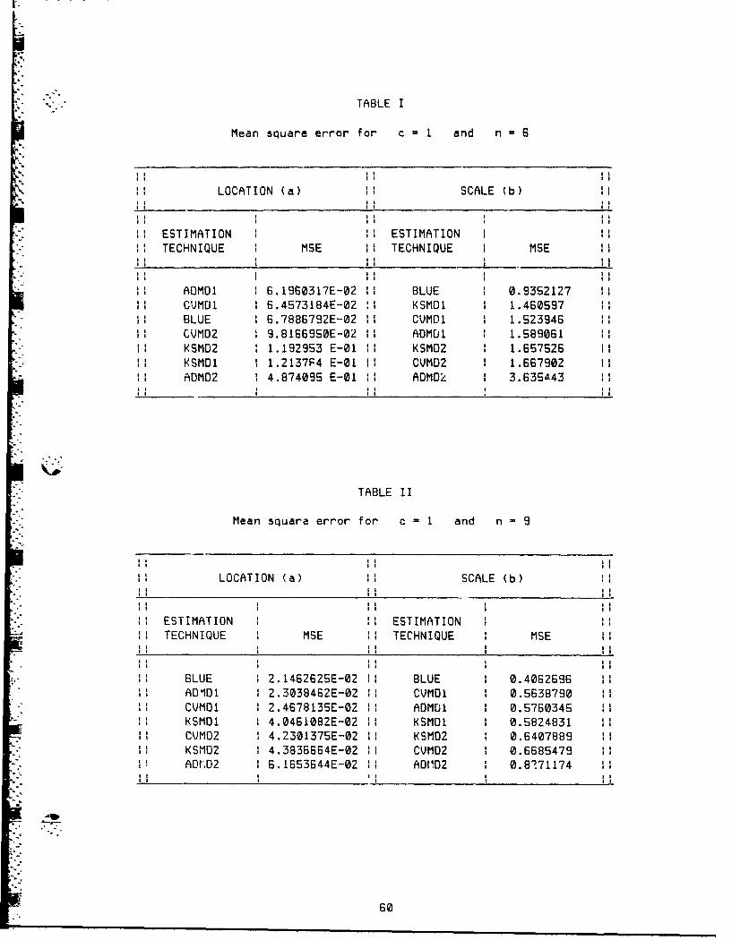
TABLE I

Mean square error for c I and n = 6

LOCATION (a) SCALE (b)

ESTIMATION 1 ESTIMATIONTECHNIQUE MSE I TECHNIQUE MSE

ADMDI 6.1960317E-02 H BLUE 1 0.9352127CvMDI 6.4573184E-02 ! KSM01 1.460597BLUE 6.7886792E-02 H CVMD1 1.523946CVMD2 1 9.81669SOE-02 !I ADMDI 1 1.589061KSMD2 1.192953 E-01 H KSMD2 1.657526KSMD1 1.2137P4 E-01 H CVMD2 1.667902ADMD2 4.874095 E-01 ADMDO 1 3.635L43

TABLE II

Mean square error for c I and n = 9

LOCATION (a) SCALE (b)

ESTIMATION 1 ESTIMATION 1I TECHNIQUE i MSE : TECHNIQUE I MSE

SBLUE 1 2.1462625E-02 H BLUE 1 0.4062696ADIDO I 2.3038462E-02 I: CVMDI 0.5638790

: CVMDI 1 2.4678135E-02 H ADMDI 1 0.5760345i KSMDI 1 4.0461082E-02 1 KSMDI 0.5824831i CVMD2 1 4.2301375E-02 I KSMD2 1 0.6407889

SKSMD2 1 4.3836664E-02 :1 CVMD2 i 0.66854791! AOtD2 I 6.1653644E-02 11 AD1O02 0.8771174

60

TABLE III

Mean square error for c I I and n - 12

LOCATiON (a) ii SCALE (b)

I ESTIMATION 1 ESTIMATIONTECHNIQUE i MSE 11 TECHNIQUE MSE

BLUE 1 1.0628480E-02 H BLUE i 0.3627600ADMDI 1 1.1631799E-02 H CVMDI 1 0.4933714CVMDI 1.3175875E-02 H ADMODI1 0 5042603CVMO2 1 2.24BS68SE-02 KSMD2 0 5136845

i KSMDI 1 2.3550959E-02 H KSMDI 1 0.5234504KSMD2 : 2.4744846E-02 !I CVMD2 1 0.5422385AOMO2 3.29776S2E-02 I ADM02 0.638002S

TABLE IV

Mean square error for c = I and n IS

"ii LOCATION (a) SCALE (b)

1- ESTIMATION 1 ESTIMATION1 TECHNIQUE MSE 11 TECHNIQUE MSE

BLUE 7.4139438E-03 11 BLUE 0.30S3709ii OMODI 9.569488SE-03 CVMDI 0.3754165CVMDI 1 1.1153221E-02 H ADMDI 0.3911322KSMDI 1.6373332E-02 KSMDI 1 0.4156374KSMD2 2.4338266E-02 I CVMD2 0.5204881CVMD2 1 2.5020871E-02 I KSMD2 0.5390435

ii ADMD2 1 2.9120248E-32 :1 ADM02 i 0.6280289

61

TABLE V

Mean square error for c I and n = 18

LOCATION (a) SCALE (b)

ESTIMATION 1 ESTIMATION11 TECHNIQUE 5 6MSE -0 TECHNIQUE MSE

BLUE 4.3005478E-03 H BLUE 1 0.1737252ADMDI 5.2362322E-03 CuMOI 0.2037124CUMDI 8 6.4189113E-03 H KSMDI 0.2041911ADMD2 8.6196102E-03 H ADMDI 0.2043972KSMDI 1.0911038E-02 H KSMD2 0.2185375

CVMD2 1 1.1255259E-02 H CVM02 1 0.2299257KSMD2 1.2906388E-02 H AOMD2 1 0.2362998

TABLE VI

Mean square error 'or c 2 and n = 6

LOCATION (a) SCALE (b)

ESTIMATION 1 ESTIMATION 1I TECHNIQUE i MSE TECHNIQUE MSE

BLUE 1.1706045E-02 H BLUE 0.5737305i DMD1 1 .2802768E-02 H KSM11 0.7080300CVMDI 1.3687569E-02 H CVMD1 0.7609550KSMOI i 1.5005208E-02 H CVMD2 0.7871752CVMO2 1 1.7071828E-02 H ADMOI 0.8051341

!I KSMD2 1 2.2394231E-02 I KSMD2 0.9329775AOM02 1 2.8150991E-02 H ADM02 i 1.161503

62

•'-."TABLE VII

Mean square error for c -2 and n 9

LOCATION (a) SCALE (b)

!lESTIMATION 1 1ESTIMATION11TECHNIQUE MSE 11TECHNIQUE i MSE

:1 BLUE 14.6055736E-03 1! BLUE 1 0.2564761ADMDI 15.1687085E-03 11 KSMD2 1 0.2969004

ii CVMDl 5 .9630712E-03 !I CVMDI 0.3137060!l CVM02 16.9629692E-03 1: KSMDI 1 0.3169191i: KSMDI 6.9843503E-03 11 CVM02 1 0.3197137i: KSMD2 17.8367852E-03 11 AOMDI 1 0.3233747

AOMO2 18.9378590E-03 11 AOMO2 1 0.4040874

.• TABLE VIII

" Mean square error for c =2 and n =12

SLOCATION (a) i:SCALE (b)

• . ESTIMATION 1 1ESTIMATION1 TECHNIQUE MSE 11TECHNIQUE MSE

ii BLUE 11.9467097E-03 11 BLUE 1 0.1996142:1 AOMDI 12.2874754E-0 KSMD2 1 0.2196842

CVMDI 2.9733009E-03 11 ADMDI 0.2351739i! ADMD2 13.0276354E-03 :1 CVMOI 0.2386533

KSMOI 13.4914461E-03 !I KStiDl 0.2393236ii CVMD2 13.7764474E-03 11 CVM02 i 0.24093S1ii KSMD2 14.6899226E-03 AOMD2 i 0.2438605

63

L•

TABLE IX

Mean 5quare error for c 2 and n 15

III

LOCATION (a) iiSCALE (b) I

BLU TB IX B'I ESTIMATION IESTIMATION I

TECHNIQUE I MSE TECHNIQUE MSE

BLUE 1.23630E-03 H LUE 1 0.16228ADMD1 1 1.4S23189E-03 H1 CvM0I 1 0.1976B05

H C'JMDI 1.954654@E-03 H1 AOMDI 0.1981037 HAOM02 1 2.OS40049E-03 H1 KSMDI 0.2068403 HKSMOI 2.317846SE-03 H CVMD2 0.2084063 HCVMD2 2.6572768E-03 KSMD2 0.2095122KSM02 13.2B47996E-03 II ADMD2 1 0.2135706

TABLE X

Mean square error for c = 2 and n 18

LOCATION (a) SCALE (b)

ESTIMATION I 11 ESTIMATION I

TECHNIQUE MSE I TECHNIQUE MSE

BLUE 7.7167596E-04 H BLUE 0.1260424ADMDI 9.3843893E-04 KSMD2 0.14010S4ADM02 1.3170647E-03 H ADMDI 0.1430691CVMDI 1.3989438E-03 H CVMDI 0.1444666KSMDI I.6IS9606E-03 !I CVMD2 1 0.1470691CVMD2 I 1.8582337E-03 :1 KSMDI 1 0.1481810KSMD2 I 2.3905281E-03 11 ADMD2 1 0.1504120

64

TABLE XI

Mean square error for c 3 and n = 6

LOCATION (a) i SCALE (b)

ESTIMATION 1 ESTIMATIONI TECHNIQUE MSE I TECHNIQUE MSE

BLUE 4.6162526E-03 H BLUE 0.3430938ADMDI 4.7417325E-03 KSMD2 0.3799514 HCVMDI 1 4.9956846E-03 KSMD1 1 0.4261144 HCVMD2 5.5936114E-03 H CVMD2 1 0.4292807 HKSMD1 1 5.6171883E-03 :1 CVMOD 0.4521263

i KSMD2 1 6.1545176E-03 H ADMOI 1 0.4634998H ADMD2 1.7377743E-02 H ADMD2 1 0.7602041 H

TABLE XII

Mean square error for c 3 and n = 9

LOCATION (a) SCALE (b)

ESTIMATION 11 ESTIMATION iTECHNIQUE MSE 11 TECHNIQUE 1SE

BLUE 2.5504350E-03 H BLUE 0.2173062 HAMDMl 2.9328801E-03 H KSMD2 1 0.2343150CVMDI 1 3.2298244E-03 I CVMD2 0.2613097

ii KSMDI 13.4083289E-03 1: CVMOI 0.2633SS1 t

CVMD2 3.4843122E-03 I KSMDI 0.26476872 A2M2 3.62043S0E-03 AOMD 0.2666046

KSMD2 3.8682341E-03 11 AOMD2 0.2911893

65

"V.

,.., TABLE XIII

tMean square er'ror for c = 3 and n = 12

LOCATION (a) il SCALE (b)

"1 ESTIMATION 1 11 ESTIMATION 11! TECHNIQUE MSE I TECHNIQUE i MSE

ill BLUE 1 .1032750E-03 H BLUE 0.146S466H ADMOl 1 .3244717E-03 H KSMD2 1 0.1634654"H1 ADMD2 I S484567E-03 H CVM02 0.1717137

CVMDI I 1.6325671E-03 It ADMOl 1 0.1786888CVMD2 1.8109ISSE-03 H CVMDI 0.1787402

H KcMDI .824S766E-03 H ADMD2 1 0.1813732KSMD2 1 2.1554409E-03 H KSMOI 1 0.1881933

TABLE XIV

Mean square error for c 3 and n = 15

LOCATION (a) ii SCALE (b)

1 ESTIMATION I ESTIMATION 1It TECHNIQUE MSE It TECHNIQUE MSE

il BLUE 1 6.1996793E-04 1: BLUE 1 0.1280874" " ADMDI 1 8.2581321E-04 H ADMOI 0.14S4654is ADM02 1 1.0506152E-03 11 CvMD1 0.1467468

CVMD1 1 1.0802834E-03 1: KSMD2 0.148421171 KSMOI 1 1.27378SOE-03 11 KSMDI I 0.1519526i CVMD2 I 1.2966762E-03 It CVMD2 1 0.1521726I: KSMD2 1 1.3728395E-03 It ADM02 i 0.1S80111

66

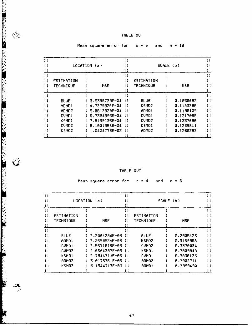
"TABLE XV

Mean square error for c 3 and n - 18

LOCATION (a) ii SCALE (b)

- ESTIMATION 1 ESTIMATION 1I TECHNIQUE I MSE I TECHNIQUE i MSE

BLUE 1 3.5388739E-04 11 BLUE 0.1050092ADMOI 1 4.7279926E-04 H KSMD2 0.1183296ADMO2 S.8612920E-04 H ADMOI 0.1190109CVMDI 6.739499SE-04 H CVMO1 1 0.121709S

: KSMD1 1 7.9139235E-04 I CVMD2 1 0.1237090CVMD2 1 8.1001956E-04 H KSMO1 0.1239811KSMO2 1 1.0424773E-03 H ADMD2 0.12S0392

TABLE XVI

Mean square error for c 4 and n 6

a LOCATION (a) SCALE (b)

ESTIMATION 1 1ESTIMATION:1TECHNIQUE i MSE 11TECHNIQUE MSE

i: BLUE 12.2004284E-03 1: BLUE 0.2905423ADMDI 2.3699524E-0 KSMD2 1 0.3169968cvmDl 2.5671816E-03 :1 CVM02 i 0.3370034CUMD2 12.6604387E-03 11 KSMBI 1 0.3809848

ii KSMDI 2.7944316E-03 1: CUMDI 0.3836123il AOMD2 13.0173361E-0 AOM02 0,3902711ii KSMD2 13.1S44713E-03 :1 ADMDI 0.3999490

Z67

a a?

"TABLE XVII

Mean square error for c 4 and n = 9

LOCATION (a) i SCALE (b)

II ~ii aI ESTIMATION a I ESTIMATION a

TECHNIQUE MSE 11 TECHNIQUE I MSE

BLUE 8 .8934094E-04 11 BLJE 1 0.1908786

ADMDI 1.1494281E-03 H KSMD2 1 0.2049502H CVMDO 1.398402SE-03 11 CVMD2 1 0.2244719

ADMD2 1 14030078E-03 1 ADOM2 0.2334024

CVMD2 1 1.48570BOE-03 H AOMOJI 0.2394877KSMDI I 1.5590133E-03 H CVMDI 1 0.2420758

H KSMD2 1.7792400E-03 KSMOI 1 0.2460075

TABLE XVIII

Mean square error for c - 4 and n = 12

LOCATION (a) SCALE (b)

ESTIMATION a ESTIMATIONSTECHNIQUE MSE TECHNIQUE MSE

H BLUE 4.3847732E-04 H1 BLUE 1 .14S4246 HADMO1 5 .357SG70E-04 H1 KSM02 0.1606177 H

Hi ADMD2 16.4326968E-04 :1 AOMO2 i .1745982 Hil CVMDI 7.0931221E-04 H CVMO2 0.1752S79

CVMD2 8.0394966E-04 ADMDI 0.1773998KSMO1 1 8.4389S72E-04 I CVMDI 0.184G511KSMD2 9.7926683E-04 H KSMDI 1 0.1893843

68

aM-, TABLE XIX

Mean square error for c 4 and n IS

I LOCATION (a) SCALE (b)

ESTIMATION a ESTIMATION a

* TECHNIQUE MSE 11 TECHNIQUE i MSE

BLUE 2.8805208E-04 H BLUE 1 0.1210762mm ADMDI 1 3.7486354E-04 H KSMD2 0.131854211 ADMD2 1 4.3274325E-04 I CVMD2 0.1393966ii CVMDI I S.3938437E-04 ADMOD2 1 0.1417205am CVM02 1 6.09273BSE-04 H ADMOI i 0.1437690!l KSMOI 6.2738BB3E-04 H CVMDI 1 0.1477181:1 KSMD2 7.4160466E-04 H KSMDI 0.157428 m

TABLE XX

Mean square error for c = 4 and n 18

LOCATION (a) ii SCALE (b)

I ESTIMATION 1 I ESTIMATION m

TECHNIQUE MSE 11 TECHNIQUE MSE

BLUE 1.9949843E-04 I BLUE 9.3522320E-02ii ADMOl 1 2.688SI97E-04 H KSMD2 1 1.0103040E-01mm ADM02 2.9941079E-04 ADMODI 1.070693SE-01

m CUMDI 4.2770977E-04 :1 ADMD2 1.07719SOE-01CVMD2 4.5176961E-04 H CVM02 1.0861484E-01

mm KSMDI S.0622342E-04 H CVMDI 1 1.1239370E-01ii KSMD2 s 5.9582230E-04 11 KSMDI 1 1.13S7192E-01

69

:' Apoendix B

Computer Program for Estimator Comparison

The following FORTRAN computer program, BLUMD.FOR, was written to

perform the Monte Carlo analysis and to generate the mean square errors

for eac.i estimation technique investigated. Program documentation is

included within the program as comment statements to inform the reader

of the purpose of each statement or group of statements. Additionall_,

each subroutine is prefaced by extensive documentation to inform the

reader of the purpose of the subroutine, all of the variables used in

the subroutine, the input variables required, the output variables

S* generated, and the major computations performed within the subroutine to

obtain the desired outputs.

"= ~70

. -c BLUMD (BLU/MINIMUM DISTANCE) MAIN PROGRAM

S.------------------------------------------------------------------c Purpose: BLUMD calculates the best linear unbiased estimates inc addition to the six minimum distance estimatesc (based on the Kolmogorov, the Cramer-von Mises, and thec finderson-Oarling distances) for both the location andc ecale parameters of the three parameter Paretoc distribution, where the shape parameter is variedc between the integer values 1,Z,3 and 4. Sample sizesc of 6, 9, IZ, 15, and 18 are used. Pareto variates arec generated for each combination of shape parameter andc sample size. Finally, BLUMD calculates the mean squarec error for each estimate type to compare whichc estimation technique performs best.C ------------------------------------------------------------------c Variables: n = sample sizec c = shape parameterc nn = sample size symbol (varies from 1-5c representing each permissable sample size)c kkk = dummy variable used to convert nn to n byc using the formula: kkk = 3 + (nn*3)c dseed = double precision seed for the Pareto variatesc x = array of Pareto variatesc B = array of B values used to calculate the bluesc for shape greater than 2c BB = array of BB values used to calculate the bluesc for shape less than or equal to 2c 0 = constant used to calculate the blues for shapec greater than Zc Anc = constant used to calculate the blues for shapec less than or equal to Zc Bnc = constant used to calculate the blues for shapec less than or equal to Zc ablu = blu estimate of location, ac bblu = blu estimate of scale, bc aKS = Kolmogorov minimum distance estimate for ac bKS = Kolmogorov minimum distance estimate for bc aCVM = Cramer-von Mises min distance estimate for ac bCVM = Cramer-von Mises min distance estimate for bc aRD = Anderson-Darling min distance estimate for ac while holding b = bblu as constantc bAD = Anderson-Darling min distance estimate for bc while holding a = ablu as constantc aZAD = Anderson-Darling min distance estimate for ac bZAD = Anderson-Darling min distance estimate for bc alCV = Cramer-von Mises min distance estimate for ac while holding b = bblu as constantc blCV Cramer-von Mises min distance estimate for bc while holding a = ablu as constantc alKS = Kolmogorov minimum distance estimate for ac while holding b = bblu as constant"c bIKS - Kolmogorov minimum distance estimate for b. while holding a = ablu as constant

71

c sse = array of sum of squared errors for eachSc estimation technique where the true value of

c a is 1 and the true value of b is 1.

"c mse = array of mean square errors for eachc estimation technique usedc count = array of counters used to count the number ofc valid estimate values foundc anda = array of calculated A-D distance measuresc when estimating location alonec esta= array of location estimates used to minimizec the A-D distancec icnt= counter for the number of location estimates

c used to minimize the A-D distancec andb = array of calculated A-D distance measuresc when estimating scale alonec estb = array of scale estimates used to minimizec the A-D distancec icntb = counter for the number of scale estimatesc used to minimize the A-D distancec andab = array of calculated A-D distance measuresc when estimating a and b simultaneouslyc estaa = array of location estimates used to minimizec the A-D distancec estbb = array of scale estimates used to minimizec the A-D distance

Sc icntab = counter for the number of location and scalec estimates used to minimize the A-0 distanceC-------------------------------------------------------------------

c Inputs: dseed = double precision seed for Pareto variatec generationc c shape parameterc n sample size

c Outputs: mse = array of mean square errors for eachc estimation technique for each parameter underc investigation (location and scale)C-------------------------------------------------------------------

c Calculate: mse = sse/number of trials

c Variable Declc':tionscommon n,x,c,ablu,bblu,dseed,B,O,Anc,Bnc,BB,aKS,bKS,

I aCVM,bCVM,aAD,bAD,nn,count,aZAD,bZAD,anda,esta,icntI ,andb,estb,icntb,andab,estaa,estbb,icntabI ,aICV,bICV,alKS,bIKS

integer n,nn,count(4,5,14),c,kkk,icnt,icntb,icntabreal x(18),ablu,bblu,B(18),D,Anc,Bnc,BB(IB),aKS,bKS,

1 aCVM,bCVM,aRD,bAO,sse(4,S,14),mse(4,5,14),aZAD,bZAD

1 ,anda(S0),andb(S00),andab(SOO),esta(SOO),estb(SO0),I estaa(SOO),estbb(SOO),aiCV,blCV,a1KS,blKS

double precision dseedcall uerset(@,levold)dseed = 4384GZI9Zl7.d00print*,'dseed = ',dseed

7Z

do 90 i=1,4c i

do 80 j =,l18, 3n

nnl nn +Ido 40 j33=1,14

sse(c,nn,jjj)=0I40 continuedo 70 it =1,1000if ((it.eq.Z@0) .or. (it.eq.400) .or. (it.eq.600) .or.

(it.eq.800) .or. (it.eq.1000)) thenprint*,'c=',c,' ,ii',n,' iteration=,it

end ifcall PARVAR

if (c .gt. 2) thencall BCGTZcall 9LCGTZgo to 4S

end -ilcall BCLE2call BLCLEZ

45 if (ablu .eq. 0 .and. bblu .eq. 0) thengo to 70'

end ifcall KSMDcall CYMMOcall ADMDcall AD6MDcall A02MDcall CYAMOcall CYBMOcall KSAMDcall KSBMD

c Calculate the Sum of Squiared Errors58 5se(c,nn,I) = sse~c,nn,I) + (ablu - 1)4**

55e(c,nn,Z) = sse(c,nn,Z) + (bblu - **

sse(c,nn,3) = 55e(c,nn,3) + (aKS - **sse(c,nn,4) = sse(c,nn,4) + QnKS - **5se(c,nn,S) = sse(c,nn,S) + (aCVM - 1)4*25se(c,nn,6) = sse(c,nn,G) + (bCVM - **

sse(c,nn,7) = sse(c,nn,7) + (aAD - 1)4*2sse(c,nn,B) = sse(c,nn,8) + (bAD - 1)4*2sse(c,nn,9) = sse(c,nn,9) + (aZAD - *Zsse(c,nn,10) = sse(c,nn,10) + (bZAD - *2

sse(c,nn,11) =sse(c,nn,11) + (aICY - **sse(c,nn,12) = sse(c,nn,12) + (bICY - *Zsse(c,nn,13) = sse(c,nn,13) + (aIKS - *Zsse(c,nn,14) = sse(c,nn,14) + (bIKS - *Z

if (it .eq. 1000) thenc Calculate the meian square error for each estimate type

do 60 11 =1,14kkk =3 + (nn*3)

73

_ ;if (court(c,nn,ll) .eq. 0) then"print*,'count=@ for c=',c,' n=',kkk,'est=',llgo to 60

"end ifmse(c,nn,lII) = sse(c,-in,ll1)/count( c, nn, 11)

print*, 'mse=', mse(c, nn, 11), ' c=' ,c,' n=' ,kkk,' est=', 11print*,'count = ',count(c,nn,11)

60 cont i nue

end ifcontinue

Be continue90 continue

endSubroutine PARVAR

C ------------------------------------------------------------------c PLrpose- For a specified sample size, n, PARVrRc generates n random variates from a Paretoc distribution with location and scale parametersc set equal to one and the shape parameter, c,c set "o either 1,1,3 or 4.C-------------------- I-------------------------------------------------------------

c Formula: x = (1/r)**(I/c)c ---------------------------------

c Variables.c r = random numberc z = shape parameterC x = array of r'areto variates

"c n = sample sizec dseed = random number seed"C-------------------------------------------------------------------c Inputs: dseed z random number seedU c = shape parameterc n = sample sizeC--- ---------------------------------------------------------------

c uutputs: x = Frray of Pareto random variatesc ------------ ----------------.------------------- ------------------

c Calculate:c x(j) = (1/r(j)) ** (1/c)C -

C ------------------------------------------------------------------

c *** Variahie Declarationsreal r(1'3),x(I8),ablu,bblu,B(18' D,.nc,Bnc,BB(18),aKS,bKS,

1 aCVM,bCVM,dAD.;'AD,aZ.,O,bZADinteger n,c, nn,count(4,5, 14)common n,x,c, ablu,bblu,dseed,B, ,J,hncBnc,BB,aKS,bKS,

1 aCVM,bCVM,aAD,bAO,nn,coun,,aZAI?,bZADdouble precision dseeddo A j:1,n

c ** Call IMSL random riiber generator subroutine ggtbscall ggubs(dseed,n,r)

c *4* Use the inverse transform technique for Pareto vat iates

""" x(j)=(ll ( ))**(l /real(c))

10 continue

74

a,•

i c. •** Call VSRTA to sort the variates in ascending ordercall vsrta(x,n)returnendSubroutine BCLEZ

-------------------------------------------------------------------------------c Purpose: For a given sample size, n, and a specified shapec ((--I or c=Z); BCLEZ calculates the B values usedc to find the blu estimates of location and scale.c In 3ddition, it calculates the constants Anc and Bncc for the given shape and sample size.

S •C - - - - - - - - - - - - - - - - - - - - - - - - - - - - - - - - - - - -

c Variables: c = shape parameterc n = sample sizec BB = array of B values (k in number)c k = number of order statistics used; k=n-[Z/cl"r nc = product of n and cc Anc = constant in tý, formula for the blu for scalec Bnc = constant in the formula for the blu for scalec-------------------------------------------------------------------c Inputs: c = shape parameterc n = sample sizec ------------------------------------------------------------------c Outputs: BB = array of B valuesc Anc = constant in the blue for the scale parameterc Bnc = constant in the blue for the scale parameter--------- --------------------------------------------------- -------.-------c Calculate:c Anc= (c+l)(c+Z)(nc-1) / (nc-Z)(nc-c-Z)C"c Bnc = (nc-Z) / (c+Z)cc For c=1 : B(i) (1 I/n) 1 I - i/(n-l) ]

•. c

-------------------------------------------------------------------------------c *** Variable Declarations:

real nc,x(18),ablu,bblu,B(18),D,Anc,Bnc,BB(IB),aKS,bKS,I aCVM,bCVM,aAO,bAD,aZAD,bZAD

integer n,k,c,nn,count(4,5,14)"double precision dseedcommon n,x,c,ablu,bblu,dseed,B,D,Anc,Bnc.BB,aKS,bKS,

I4 1 aCVM,bCVM,aAD,bAD,nn,count,,aZAD,bZAOk~n-(Z/c)

c *** Calculate the B values w;len c=lif (c.eq.l) then

do 10 3=1,k"BB(j)=(l-3/real(n))*'l-j/(real(n)-1))

7- 1@ cont'nue"go -. 36

end ifc * Calculate the B values when c=Z (i.e., c.ne.I)

75

,* .do 20 m=l,k

BB(m)=I-m/real(n)zo continue36 nc = n * cc ** Calculate the constants Anc and Bnc

Anc= ((c+l)*(c+Z)*(nc-l)) / ((nc-Z)*(nc-c-Z))Bnc- (nc-Z) / (c+Z)returnendSubroutine BLLLEZ

C ------------------------------------------------------------------c Purpose: For a given sample size, n, and shape (c=l or c=Z),c BLCLEZ calr,.ates the best linear unbiased estimatesc of location a,,d scale for a sample of ordered ParetoC variates.c----------------------------------------------------------------------------------

c Variables: x = array of ordered Pareto variatesc c = shape parameterc n = sample sizec BB = ar-ay of B values used to calculate the bluesc nc = product of n and cc k = number of order statistics used; k = n - (Z/clc Anc = constant used to calculate the blue for scale

* c Bnc = constant used to calculate the blue for sca'.ec Bxsum = sum of [B(i) * x(i)] terms for i = 1,2,. kc ablu = blu estimate of the location parameter, ac bblu = blu estimate of the scale parameter, b I"c count = array of counters used to count the number ofc valid estimate values foundc-------------------------------------------------------------------c Inputs: x = array of ordered Pareto variatesc c = shape parameterc n = sample sizec BB = array of B values used to calculate the bluesc Anc = constant used to calculate the blue for scalec Bnc = constant used to calculate the blue for scaleC-------------------------------------------------------------------c Outputs: ablu = blu estimate of the location parameter, ac bbiu = blu estimate of the scale parameter, bS- ------------------------------------------------------------------c Calculata:c b (Anc) B(l)x(1) ' B(Z)x(Z) + + B(k)x(k)c - (Bnc)x(l) Icc a =x(l) - [ bi(nc-i) ]

c V Yariable Declarat:.ns:real x(.1),ablu,bblu,Bxsum,nc,8(l8),D,Anc,Bnc,BB(18),

I aKS,bKS,aCVM,bCVM,aAD,bAD,aZAD,bZRDinteger n,k,c,nn,count(4,5,14)double precision dsee'co,.imon n,x,c,ablu,bblL, .ieed,B,D,Rnc,Bnc,BB,aKS,bKS,

76

I aLVM,bCVM,arD,bAD,nn,count,aZAD,bZAD"Bxsum=0k=n-(Z/c)

.'. c *** Sum the products of B(i) and x(i) for i =I,Z,...kdo 10 j=t,k

Bxsum=Bxsum+BB( j )*x( j)10 continuue

ncr=n*cc *** Calculate the blue for scale, then for location

bblu=Anc*(Bxsum - Bnc*x(1))ablu=x( )-bblu/( nc-I)

c *** Increment counter for valid bluesif (bblu .gt. 0) then

"count(c,nn,l) = count(c,nn,l) + Icount(c,nn,Z) = count(c,nn,Z) + 1

elseprint*,'bblu=',bblu,'ablu=',ablu,' negativity'ablu = 0

bblu = 0end if

returnendSubroutine BCGTZ

S- ------------------------------------------------------------------c Purpose: For a given sample size, n, and a specified shape,c cOZ; BCGTZ calculates the B and D values used toc find the blu estimates of location and scale.c-------------------------------------------------------------------c Variables: c = shape parameterc n = sample sizec B = array of B values (n in size)c D = D valuec bsum = sum of B values for i=1 . (n-I)C -------------------------------------------------------------------c Inputs: c = shape parameterc n = sample sizeC-------------------------------------------------------------------c Outputs: B = array of B valuesc D = D valueC-------------------------------------------------------------------c Calculate:c B(i) = [1 - Z/c(n-i+l)] * B(1-1)cc D = (c+l)[B(l) + B(Z) + ... + B(n-1)] + (c-1)B(n)cc ------------------------------------------------------------------c *** Variable Declarations:

real bsum,x(18),ablu,bblu,B(18),D,Anc,Bnc,BB(18),aKS,b S,I aCVM,bCVM,aAD,bAD,aZAD,bZAD

integer n,c,nn,count(4,5, 14)- double precision dseed

"common n,x,c,ablu,bblu,ds eed,B,D,Anc,Bnc,BB,aKS,bKS,"I aCVM,hCVM,aAD,bAD,nncount,aZAD,bZAD

"77

c * Calculate the first B valueB(l)=(1-(2/(c*real(n))))

c * Calculate the second thru the nth B values

do 10 j=Z,nB(j )=B( j-l )*( l-( Z/(real(c)*(n-3+l))))

10 continue::~bsu m= 0

c Sum the 'first' to the 'nth minus one' B valuesdo ZO k=l,(n-1)

bsum~bsum+B( k)zo continuec *** Calculate the D value

0 = (c+l) * bsum + (c-1) * B(n)returnend

Subroutine BLCGTZc-------------------------------------------------------------------c Purpose: For a given sample size, n, and a specified shape,

. c c>Z, BLCGTZ calculates the best linear unbiasedc estimates of location and scale.

----------------- --------------------------------------------------------------c Variables: x = array of ordered Pareto variatesc c = shape parameterc n = sample sizec B = array of B values used to calcJlate the bluesc D = D value used to calculate the bluesc Y = Y value used to calculate the bluesc ablu = blu for location parameter, ac bblu = blu for scale parameter, bc Bxsum = sum of 1B(1) * x(i)] terms for i =,Z.... ,(n-1)c nc = product of n and cc count = array of counters used to count the number of

c valid estimate values found-------------------------------------------------------------------------------c Inputs: x = array of ordered Pareto variatesc c = shape parameter

c n = sample size"c B = array of B values used to calculate bluesc 0 = D value used to calculate the blues---------------------------------------------------------------- ---------------c Outputs: ablu = blu estimate for location, ac bblu blu estimate for scale, bC ------------------------------------------------------------------c Calculate:c Yla (c+l)[ B(l)x(l) + B(Z)x(Z) + ... + B(n-1)x(n-l) Ic + (c-I)[ B(n)x(n) I - Dx(I)cc a x(l) - Y/[(nc-1)(nc-Z) - Dnc]

cc b (nc-I) E x(l) - a I

-- c

-------------------------------------------------------------------------------------------c *** Variable Declarations:

78

real x(18),ablu,bblu,Bxsum,nc,Y,B(18),D,Anc,Bnc,BB(18)I ,aKS,bKS,aCVM,bCVM,taAD,bAD,aZAD,bZAD

integer n,c,nn,count(4,5,14)*" double precision dseed

common n, x, c, ablu,bblu,dseed,B,O,AncBnc,BB,aKS,bKS,1 aCVM,bCVM,aAD,bAD,nn,count,eZRD,bZAD

'w ~Bx sum =

c *.. Sum the products of the B(i) and x(i) values to i = n-Ido 10 j1l,(n-1)

Bxsum=Bxsum+B( j )*x( j)10 continuec ** Calculate the Y value

Y=( c+l )*Bxsum+( c-i )*B( n)*x( n)-D*x( 1)nc=n*c

c-*** Calculate the blu estimates for location and scaleablu=x( 1 )-Y/((nc-i)*(nc-Z)-(nc*D))bblu=( nc-i )*( x( I )-ablu)

c *** Increment counters for valid bluesif (bblu .gt. 0) then

count(c,nn,l) = count(c,nn,l) + Icount(c,nn,Z) = count(c,nn,Z) + 1

elseprint*,'ablu=',ablu,' bblu=',bblu,' negativity'ablu = 0bblu = 0

end if"returnendSubroutine KSMO

c-------------------------------------------------------------------c Purpose: KSMD generates the minimum distance estimates ofc location and scale based upon minimizing thec Kolmogorov distance measure defined in subroutinec KOIS. This routine uses the blu estimates as thec starting points for the estimate modifications.-------------------------------------------------------------------------------c Variables: NPAR = number of parameters altered by minimizingc the Kolmogorov distancec NSIG = number of significant digits for convergencec MAXFN = maximum number of function evaluationsc IOPT = options selector (see IMSL manual on ZXMIN)c H, G, W vectors defined in IMSL mar'ual on ZXMINc IER = error parameter (see IMSL manual on ZXMIN)c F = value of Kolmogorov distance at the finalc parameter estimatesc kse = Kolmogorov derived minimum distance estimatesc aKS = Kolmogorov minimum distance location estimatec bKS = Kolmogorov minimum distance scale estimatec ablu = blu estimate of locationc bblu = blu estimate of scalec count = array of counters used to count the number ofc valid estimate values foundC-------------------------------------------------------------------

79

c Inputs' NPAR = number of parameters altered while minimizingc NSIG = number of significant digits requiredc MAXXFN = maximum number of function evaluationsc IOPT = options selector (see IMSL manual on ZXMIN)c kse = initial estimates for the minimization processc ablu = blu estimate of locationc bblu = blu estimate of scaleC ------------------------------------------------------------------c Outputs: F = minimum value of the function being minimized

c kse = revised estimate valuesc aKS = revised MO estimate of location [aKS = kse(l)]c bKS = revised MD estimate of scale [bKS = kse(Z)]c H, G, W = vectors defined in IMSL manual on ZXMINc IER = error parameter (see IMSL manual on ZXMIN)c------------------------------------------------------------------

"c Calculate: no calculations performed in this subroutineS-------------------------------------------------------------------c *** Variables Declarationf

common n, x,c, ablu,bblu,dseed,B,D,Rnc,Bnc,BB, aKS,bKS,

I aCVM,bCVM,aAD,bAD,nn,count,aZAD,bZADexternal kdisinteger NPAR,NSIG,MAXFN,IOPT,n,c,nn,cnunt(4,5,14)real kse(Z),H( 3),G(Z),W(6),F,x(IB),ablu,bblu,aKS,bKS,

I B(18),D,Anc,Bnc,BB( I1),aCVM,bCVM,aAD,bAD,aZAD,bZADdouble precision dseed

c *** Enter the ZXMIN required constants

NPAR = ZNSIG = 3MAXFt = 500IOPT = 0

c *** Initialize the kse values to the blu estimateskse(l) = ablukse(Z) = bblu

c * Call ZXMIN to refine the kse values by minimizingc the Kolmogorov distance (KST) computed in thec subroutine KDIS

call ZXMIN(KDIS,NPAR,NSIG,MAXFN,IOPT,kse,H,G,F,W,IER)c *** Relabel the refined estimates of location and scale

aKS = kse(1)bKS = kse(Z)

c *** Incremrt the KS counterscount(c,nn,3) = count(c,nn,3) + 1

count(c.nn,4) = count(c,nn,4) + IreturnendSubrouu.ne KDIS(NPAR,kse,F)

C ------------------------------------------------------------------c Purpose: KDIS provides the function which is to be minimizedc by ZXMIN for the Kolmogorov distance measure. Thec location and scale parameters are altered to achievec this minimization.

c-------------------------------------------------------------------c Variables: NPAR = number of parameters available to alter

88

c n = sample sizec kse = estimates of the parameters being alteredc F = value of the function to be minimizedc x = array of ordered Pareto variates"c c = shape parameterc zi = array of Pareto cdf pointsc DP = positive differences betueen the EDF and cdfc OM = negative differences between the EDF and cdfc DPLUS = maximum positive differencec DMINUS = maximum negative differencec KST = Maximum of OPLUS and DMINUSC ------------------------------------------------------------------

c Inputs: NPAR = number of parameters available to alterc n = sample sizec kse = initial estimates (the blu estimates)c x = array of ordered Pareto variat5sc c = shape parameterc------------------------------------------------------------------c Outputs' F = value of the function at the final estimatesc kse = revised estimates of location and scale;c these are the Kolmogorov minimum distancec estimatesc-------------------------------------------------------------------

c Calculations:c z(i) 1 - (I + [x(x)-a]/b)**(-c)

c OP(i) = ABSE i/n - z(i) ]cc OM(i) = ABS[ z(U) - (i-1)/n IcC ------------------------------------------------------------------c * Variable Declarations:

common n, x, c, ablu,bblu, dseed, B, D, Anc, Bnc, BB, aKS, bKS,I aCVM,bCVM,aRD,Bad,nn,count,aZAD,bZAD

integer NPAR,n,c,nn,count(4,5,14)real kse(NPAR),F,x(18),zi(18),DP(IB),DM(18),DPLUS,

I DMINUS,KST,ablu,bblu,B(18),D,Anc,Bnc,BB(IB),aKS,bKS,1 aCVM,bCVM,aAD,bAD,aZAD,bZAD

double precision dseedc *** Calculate the Pareto cdf value [zi(j)] at each pointc and the difierences between the EOF step functionc and the cdf points

do 10 j=l,nzi(j) = l-(Il(l+(x(j)-kse(1))/kse(Z)))**c

DP(j) = ABS(j/real(n) - zi(j))

DM(j) = ABS(zi(j) - (j-1)/real(n))10 continuec * Select the maximum of the plus and minus differences

(PLUS = MAX(DP(1),DP(2),DP(3),DP(4),DP(S),DP(6),DP(7)I ,OP(8),OP(9),DP( I),DP( II),OP( IZ),DP( 13),OP(14)

- I , DP(15),DP(l6),DP(17),DP(18))

DMINUS = MAX(DM(1 ),DM(Z),DM(3),DM(4),DM(5),DM(6),ODM,(7)1,DM(8),r)M(9),DM( 10),DM(1l),DM(IZ),DM(13),DM(14)

81

: &* I ,OM(lS),DM(16),DM(17),OM(18))c *** Select the maxir•jm Kolmogorov distance measure andc set F equal to that distance. F becomes thec function which ZXMIN attempts to minimize byc altering the values of the location and scalec parameters

KST = MAX(DPLUS,DMINUS)

F =KSTreturnendSubroutine CVMMD

c ------------------------------------------------------------------c Purpose: CVMMD generates the minimum distance estimates ofc location and scale based upon minimizing thec Cramer-von Mises distance measure defined in subroutinec CVMDIS. This ro'jtine uses the blu estimates as thec starting points for the estimate modifications.C ------------------------------------------------------------------

c Variables: NPAR = number of parameters altered by minimizingc the Cramer-von Mises (CVM) distancec NSIG = number of significant digits for convergencec MAXFN = maximum number of function evaluationsc IOPT = options selector (see IMSL manual on ZXMIN)c H, G, U = vectors defined in IMSL manual on ZXMINc IER = error parameter (see IMSL manual on ZXMIN)c F = value of CVM distance at the finalc parameter estimatesc cvme = CVM derived minimum distance estimatesc aCVM = CVM minimum distance location estimatec bCVM = CVM minimum distance scale estimatec ablu = blu estimate of locationc bblu = blu estimate of scalec count = array of counters used to count the number ofc valid estimate values foundC ------------------------------------------------------------------c Inputs: NPAR = number of parameters altered while minimizingc NSIG = number of significant digits requiredc MAXFN = maximum number of function evaluationsc IOPT = options selector (see IMSL manual on ZXMIN)c cvme = initial estimates for the minimization processc ablu = blu estimate of locationc bblu = blu estimate of scalec -------------------------------------------------------------------c Outputs: F = minimum value of the functio!. being minimizedc cvme = revised estimate valuesc aCVM = revised MD estimate of location [aCVM=cvrie(1)]c bCVM = i-evised MD estimate of scale [bCVM=cvme(Z)]c H, G, W = vectors defined in IMSL manual on ZXMINc IER = error parameter (see IMSL manual on ZXMIN)c -------------------------------------------------------------------c Calculate: no calculations performed in this subroutinec---------------------------------------------------------------------------

8Z

c *.* Variables Declaration:common n,x,c,ablu,bblu,dseed,B,D, Anc,Bnc,BB,aKS,bKS,

I aCVM,bCVM,aRD,bAD,nn,count,aZAD,bZADexternal cvmdi5integer NPAR,NSIG,MRXFN,IOPT,n,c,nn,count(4,5,14)real cvme(Z),H(3),G(Z),t(6),F,x(IB),ablu,bblu,aCVM,bCVM

I ,B(18),D,Anc,Bnc,BB(I8),aKS,bKS,aAD,bAD,aZAD,bZADdouble precision dseed

c *** Enter the ZXMIN required constantsNPAR = ZNSIG = 3%MAXFN 500IOPT = 0

c *** Initialize the cvme values to the blu estimatescvme(1) = ablucvme(Z) = bblu

c ** Call ZXMIN to refine the cvme values by minimizingc the CVM distance (WZ) computed in thec subroutine CUMDIS

call ZXMIN(CVMDIS,NPAR,NSIG,MAXFN,IOPT,cvme,H,G,F,W,IER)c *** Relabel the refined estimates of location and scale

aCVM = cvme(1)bCVM = cvme(Z)

c * Increment the CVM counterscount(c,nn,5) = count(c,nn,5) + 1count(c,nn,6) = count(c,nn,6) + IreturnendSubroutine CVMDIS(NPAR,cvme,F)

-----------------------------------------------------------------------------c Purpose: CVMDIS provides the function which is to be minimizedc by ZXMIN for the Cramer-von Mises distance measure.c The location and scale parameters are altered toc achieve this minimization.-----------------------------------------------------------------------------c Variables: NPAR = number of parameters available to alterc n = sample sizec cvme = estimates of the parameters being alteredc F = value of the function to be minimizedc x = array of ordered Pareto variatesc c = shape parameterc zi = array of Pareto cdf pointsc ACV = the squared quantity in the WZ formulac SCVM = the sum of the ACV quantitiesc WZ = the CVM distance measurec . . . . . . . . . . . . . . . . . . . . . . . . . .c Inputs: NPAR = number of parameters available to alterc n = sample sizec cvme = initial estimates (the blu estimates)c x = array of ordered Pareto variatesc c = shape parameter

83

c Outputs: F = value of the function at the final estimatesc cvme = revised estimates of location and scale;c these are the CVM minimum distance estimatesC --..................................................................

c Calculations:c z(i) = I - (1 + [x(i)-a]/b)**(-c)c

c ACV(i) = E z(i) - (Zi-1)/Zn ]**Z

c

c SCVM = ACV(l) + ACV(Z) + ... + ACV(n)cc WZ = SCVM + 1/lZncC . .

------------------------------------------------------------------------------------------------

c * Variable Declarations:common n, x,c,ablu,bblu,dseed,B,D,Anc,Bnc,BB, aKS,bKS,

I aCVM,bCVM,aAD,bAD,nn,countaZAD,bZADinteger NPAR,n,c,nn,count(4,5,14)real cvme(NPAR),F,x(IB),zi(18),SCVM,ACV(18),WZ

I , ablu,bblu,B( 18),D,Anc,Bnc,BB( 18),aKS,bKS,aCVM,bCVM,1 aAD,bAD,aZAD,bZAD

double precision dseedSCVM = 0do 10 j=l,n

zi•2) = l-(I/(1+(x(j)-cvme(1))/cvme(Z)))**cACV(j) (zi(j) - (Z*j-l)/(Z*real(n)))**ZSCVM = SCVM + ACV(j)

10 continueWZ = SCVM + (1/(IZ*real(n)))F WZreturnendSubroutine ADMO

c-------------------------------------------------------------------c Purpose- ADMO generates the minimum distance estimates ofc the location parameter based upon minimizing the, Anderson-Darling distance measure defined inc subroutine ADDIS. ADMO uses the blu estimates as thec starting points for the estimate modifications.c-------------------------------------------------------------------c Variables: NPAR = number of parameters altered by minimizingc the Ande5son-Darling (A-D) distancec NSIG = number oi significant digits for convergencec MAXFN = maximum number of function evaluationsc IOPT = options selector (see IMSL manual on ZXMIN)c H, G, W = vectors defined in IMSL manual on ZXMINc IER = error parameter (see IMSL manual on ZXMIN)c F = value of A-D distance at the finalo parameter estimatesc ade = A-D derived minimum distance estimate

84

c aUD = A-D minimum distance location estimatec ablu = blu estiMate of locationc bblu = blu estimate of scalec count = array of counters used to count the number ofc valid estimate values foundc anda = array of calculated A-0 distance measuresc esta = array of location estimates used to minimizec the A-D distance measurec icnt = counter for the number of estimates usedc ------------------------------------------------------------------"c Inputs: NPAR = number of parameters altered while minimizingc NSIG = number of significant digits requiredc MAXFN = maximum number of function evaluationsc IOPT = options selector (see IMSL manual on ZXMIN)c ade = initial estimate for the minimization processc ablu = blu estimate of locationc bblu = blu estimate of scaleC ------------------------------------------------------------------c Outputs: F = minimum value of the function being minimizedc ade = revised estimate valuesc aAD = revised MD estimate of location [aAD = ade(l)]c H, G, W = vectors defined in IMSL manual on ZXMINc IER = error parameter (see IMSL manual on ZXMIN)c ------------------------------------------------------------------c Calculate- no calculations performed in this subroutineS-----c *** Variables Declaration:

common n,x,c,ablu,bblu,dseed,B,DAnc,Bnc,BB,aKS,bKS,1 aCVM,bCVM,aAD,bAD,nn,count,aZAD,bZAD,anda,esta,icnt1 ,andb,estb,icntb,andab,estaa,estbb,icntab

external addis"integer NPAR,NSIG,MAXFN,IOPT,n,c,nn,count(4,5,14),icnt,hh

I ,icnib,icntabreal ade(l),H(1),G(l),W(3),F,x(18),ablu,bblu,aAD,bAD

I ,B(18),D,Anc,Bnc,BB(18),aKS,bKS,aCVM,bCVM,aZRO,bZADI ,anda(S00),esta(SOO),ADI,andb(50),estb(SOO),ardab(500)1 ,estaa(S0O),estbb(SOO)

double precision dseedc Enter the ZXMIN required constants

NPAR = INSIG = 3MAXFN 500IOPT = 0

c Initialize the ade value to the blu estimateade(1) = ablu

c * Call ZXMIN to refine the ade values by minimizingc *** the Anderson-Darling distance (AD) computed inc the subroutine ADOIS

call ZXMIN(ADDIS,NPAR,NSIG,MAXFN,IOPT,ade,H,G,F,W,IER)aRD ade(1)

c ** Reinitialize the icnt, anda, and esta arrays

1• 85

• 25 icnt 0do 30 1 l,W(Z)

anda(i) = 0esta(i) = 0

30 continuec *** Increment AD counter for valid AD estimates

count(c,nn,7) = count(c,nn,7) + IreturnendSubroutine ADDIS(NPAR,ade,F)

c-------------------------------------------------------------------c Purpose: ADDIS provides the function which is to be minimizedc by ZXMIN for the Anderson-Darling distance measure.c The location parameter is altered to achieve thec minimization.------------------------------------------------------------------------------c Variables: NPAR = number of parameters available to alterc n = sample sizec ade = estimates of the parameter being alteredc F = value of the function to be minimizedc x = array of ordered Pareto variatesc c = shape parameterc zi = array of Pareto cdf pointsc ARA = array of terms to be summed in AD formulac SAAD = sum of the AAA(i) termsc AD = Anderson-Darling distance measurec anda = array of calculated A-D distance measuresc esta array of location estimates used to minimizec the A-D distance measurec icnt = counter for the number of estimates usedC ------------------------------------------------------------------c Inputs: NPAR = number of parameters available to alterc n = sample sizec ade = initial estimate (the blu estimate)c x = array of ordered Pareto variatesc c = shape parameterC------------------------------------------------------------------c Outputs: F = value of the function at the final estimatec ade = revised estimate of location; this is thec Anderson-Darling minimum distance estimateC ------------------------------------------------------------------c Calculations:c z(i) = I - (I + [x',i)-a]/b)**(-c)

c AAA() = (Zi-1) [ in zl1) + ln ( l-z(n+l-i) ) Icc SAAD = AAM(l) + AAA(Z) + . + AAA(n)cc AD = (-SAAD)/n - nC

' • C . .. . . . .. .. . . .. . . . . . . . . . . 8.

c *** Variable Declarations:common n,x,c,ablu,bblu,dseed,B,D,Anc,BBnc,BB,aKS,bKS,

I aCVM,bCVM,aAD,bAD,nn,count,aZAO,bZAD,anda,esta,icnt"I ,andb,estb,icntb,andab,estaa,estbb,icntab

integer NPAR,n,c,nn,count(4,S,14),icnt,zcntb,icntabreal ade(NPAR),F,x(18),zi(18),AAA(I8),SAAD,AD

1 ,ablu,bblu,B( 18),D,Rnc,Bnc,BB(18),aKS,bKS,aCVM,bCVM,1 aAD,bAD,aZAD,bZAD,anda(500),esta(S00)I ,andb(S00),estb(500),ancab($00),estaa(500),estbb(500)

double precision dseeddo 10 j=1,n

c *** Calculate the Pareto cdf point valueszi(j) = 1-(l/(1+(x(j)-ade(1))/bblu))**c

"c *** Test zi(j) and I I - zi(j) ] for negativityif (zi(j).le.0 .or. zi(j).ge.1) then

go to 30end if

10 continue"SARAD = 0

c *** Calculate the Anderson-Darling distancedo 20 m=l,n

AAA(m) = (Z*,m-1) * (log(zi(m)) + log(l-zi(n+l-m)))SAAD = ShAD + AAA(m)

20 continue0D = (-I) * (n + SAAD/n)

c *** Save the AD and ade(l) valuesicnt = icnt 4 1anda(icnt) = ADesta(icnt) = ade(l)

c *** Relabel the A-D distanceF = ADgo to 40

30 ade(1) = esta(icnt-1)40 return

endSubroutine ADBMD

C ------------------------------------------------------------------c Purpose: ADBMD generates the minimum distance estimates ofc the scale parameter based upon minimizing thec Anderson-Darling distance measure defined inc subroutine ADBDIS. AOBMD uses the blu estimates as thec starting points for the estimate modifications.C ---------- *----------------------------------------------------------c Variables: NPAR = number of parameters altered by minimizingc the Anderson-Darling (A-D) distancec NSIG = number of significant digits for convergencec MAXFN = maximum number of function evaluationsc IOPT = options selector (see IMSL manual on ZXMIN)c H, G, W = vectors defined in IMSL manual on ZXMINc IER = error parameter (see IMSL manual on ZXMIN)c F = value of A-D distance at the final

87

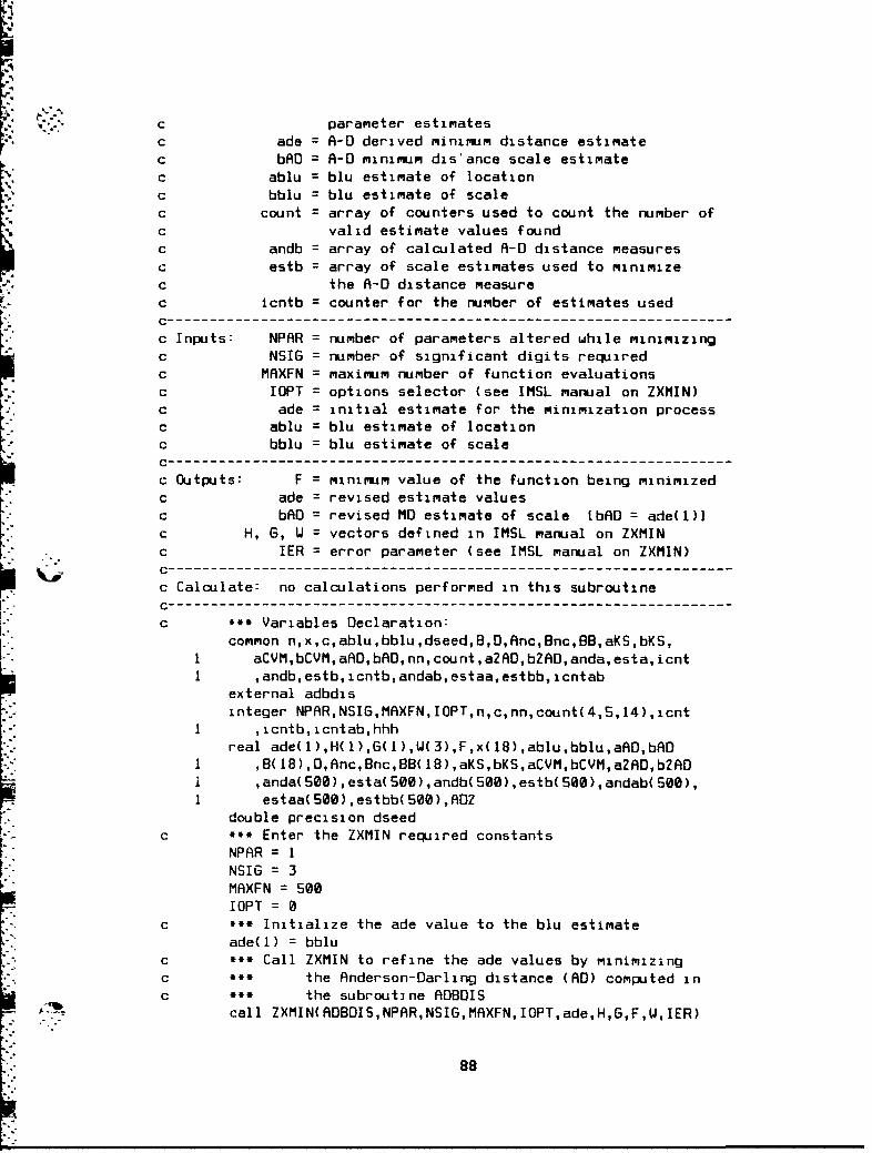
c parameter estimatesc ade = A-D derived minimum distance estimatec bAD = A-D minimum dis'ance scale estimatec ablu = blu estimate of locationc bblu = blu estimate of scalec count = array of counters used to count the number ofc valid estimate values foundc andb = array of calculated A-D distance measuresC estb = array of scale estimates used to minimizec the A-D distance measurec icntb = counter for the number of estimates usedc-------------------------------------------------------------------

c Inputs: NPAR = number of parameters altered while minimizingc NSIG = number of significant digits requiredc MAXFN = maximum number of function evaluationsc IOPT = options selector (see IMSL manual on ZXMIN)

c ade = initial estimate for the minimization processc ablu = blu estimate of location

c bblu = blu estimate of scaleC ------------------------------------------------------------------

c Outputs: F = minimum value of the function being minimized

c ade = revised estimate valuesc bAD = revised MD estimate of scale [bAD = ade(l)]c H, G, W = vectors defined in IMSL manual on ZXMIN

-" c IER = error parameter (see IMSL manual on ZXMIN)

------------------------------------------------------------------------------c Calculate: no calculations performed in this subroutine

------------------------------------------------------------------------------c *** Variables Declaration:

common n,x,c,ablu,bblu,dseed,B,D,Anc,Bnc,BB,aKS,bKS,1 aCVM,bCVM,aAD,bAD,nn,count,aZAD,bZAD, anda,esta, icnt1 ,andb,estb,icntb,andab,estaa,estbb,icntab

external adbdisinteger NPAR,NSIG,MAXFN,IOPT,n,c,nn,count(4,5,14),icnt

I ,icntb,icntab,hhhreal ade(1),H(l),G(l),W(3),F,x(18),ablu,bblu,aAD,bAD

I ,B(18),D,Anc,Bnc,BB(18),aKS,bKS,aCVM,bCVM,aZAD,bZADi ,anda(S00),esta(S00),andb(SOO),estb(SOO),andab(500),I estaa(S00),estbb(S00),ADZ

double precision dseedc *'* Enter the ZXMIN required constants

NPAR = INSIG = 3MAXFN 500IOPT = 0

c * Initialize the ade value to the blu estimateade(l) = bblu

c *** Call ZXMIN to refine the ade values by minimizingc the Anderson-Darling distance (AD) computed in

"c the subroutine ADBDIScall ZXMIN(ADBDIS,NPAR,NSIG,MAXFN,IOPT,ade,H,G,F,W,IER)

88

bPD =ade(l)4 .

c **. Reinitialize the icntb, andb, and estb arraysZ5 icntb = 0

do 30 1 = l,W(Z)andb(i) = 0estb(i) = 0

30 continuec *** Increment AD counter for valid AD estimates

count(c,nn,8) = count(c,nn,B) + Ireturnend"Subroutine ADBDIS( NPAR, ade, F)

C -------------------------------------------------------------------c Purpose: ADBDIS provides the function which is to be minimizedc by ZXMIN for the Anderson-Darling distance measure.c The scale parameter is altered to achieve theC minimization.c-------------------------------------------------------------------c Variables: NPAR = number of parameters available to alterc n = sample sizec ade = estimates of the parameter being alteredc F = value of the function to be minimizedc x = array of ordered Pareto variatesc c = shape parameterc zi = array of Pareto t'f pointsc ARA = array of terms to be summed in AD formulac SAAD = sum of the AAA(i) terms

c AD = Anderson-Darling distance measure"c andb = array of calculated A-D distance measuresc estb = array of scale estimates used to minimizec the A-D distance measurec icntb = counter for the number of estimates used

c Inputs: NPAR = number of parameters available to alterc n = sample sizec ade = initial es'imate (the blu estimate)c x = array of ordered Pareto variatesc c = shape parameterC ------------------------------------------------------------------c Outputs: F = value of the function at the final estimate

c ade = revised estimate of scale; this is thec Anderson-Oarling minimum distance estimatec ------------------------------------------------------------------c Calculations:c z(i) = 1 - (I + [x(i)-a]/b)**(-c)cc AAA(i) (Zi-l) [ In z(i) + In ( 1-z(n+l-i ) Icc SAAD = AAA(l) + AAAM(Z) + + AAA(n)

7 c AD = (-SAAD)/n - n

89

Lc *** Variable Declarations:

common n,x,c,ablu,bblu,dseed,B,D,Anc,Bnc,BB,aKS,bKS,I aCVM,bCVM,aAD,bAD,nn,count,aZAD,bZAD,anda,esta,icnt1 ,andb,estbicntb,andab,estaa,estbb,icntab

integer NPAR,n,c,nn,count(4,S,14),icnt,icntb,icntabreal ade(NPAR),F,x(18),zi(lB),AAA(I8),SAAD,AD

I ,ablu,bblu,B(18),DAnc,Bnc,B8(18),aKS,bKS,aCVM,bCVM,1 aAD,bAD,aZAD,bZAD

1 ,anda(SOO),esta(SOO),andb(500),estb(S08),andab(508),I estaa(500),estbb(500)

double precision dseed

do 10 j=l,nc * Calculate the Pareto cdf point values

zi(j) = 1-(l/(l+(x(j)-ablu)/ade(l)))**cc * Test zi(j) and [ I - zi(j) I for negativity

if (zi(j).le.0 .or. zi(j).ge.l) thengo to 30

end if10 continue

SAAD = 0

c * Calculate the Anderson-Darling distancedo ZO m=l,n

AAA(m) = (Zfm-I) * (log(zi(m)) + log(l-zi(n+l-m)))SAAD -SAAD0 + AAA( M)

2 ra coniinueAD - (-1) * (n t SAADin)

c *** Save the AD and ade(l) values

icntb - icntb T iandb(icntb) - ADestb(icntb) - ade(1)

c ** Relabel the A-D distancer - flu

go to 4630 ade(i) - esibhicntb-i)406 return

endSubroutine ADZMD

c -------------------------------------------------------------------Purpose- mDZaD generates the minimum distance estimates of

c location and scale simuitaneously, based on minimizingc the Anderson-Darling distance measure defined inc subroutine ADZDiS. ANDZD uses the blu estimates as thec starting points for the estimate modifications.C ------------------------------------------------------------------

c Variables- NFAR - number of parameters altered by minimizingc the Anderson-Darling ,A-D) distancec NSIG - number of significant digits for convergencec I'MAXFN - maximum number of function evaluationsc lOFT - options selector (see IiSL manual on ZXMIN)

96

" "' c H, G, U vectors defined in IiSL manuai on ZXMIN

c iER - error parameter (see iH5L manual on Z7iIN)

c F - value of A-D distance at the finalc parameter estimates

c ade - 0-D derived minimum distance estimateSc aZAD - A-D minimum distance location estimate

c bZAD - A-D minimum distance scale estimate

c ablu - blu estimate of locationc bbiu - biu estimate of scalec count - array of counters used to count the number ofc valid estimate values foundc andab - array of calculated A-D distance measuresc estaa - array of location estimates used to minimizec the A-D distance measurec estbb - array of scale estimates used to minimizec the A-D distance measure

c icntab - counter for the number of estimates usedc------------------------------------------------------------------c inputs. NPAR - number of parameters altered while minimizingc NSIG - number of significant digits requiredc MAXFN - maximum number of function evaluationsc !OPT - options selector (see IMSL manual on ZXHIN)c ade initial estimate for the minimization processc abju - blu estimate of location

c bblu - blu estimate of scale-----------------------------------------------------------------------------c Outputs- F minimum value of the function being minimizedc ade - revised estimate valuesc aZAD - revised HD estimate of location iaZAD - ade(I)ic bZAD - revised nD estimate of scale (bZAD - ade(Z)]c G, W, w - vectors defined in IHSL manual on ZXHINc iER - error parameter (see iHSL manual on ZXiIN)c ------------------------------------------------------------------c Calculate. no calculations performed in this subroutine

c-------------------------------------------------------------------• c -- Variables Declaration.

common n,x,c,ablu,bblu,dseed,B,D,Anc,Bnc, BB, aKS,bKS,i aCVH,bCVn,auD,bAD,nn,count,aZAD,bZAD,anda,esta,icnti ,andb,estb,icntb,andab,estaa,estbb,icntab

external adZdis

integer NPAR,NSIG,niAXFN,IuPT,n,c,nn,count(4,5,i4)K ,icnt,icnib,icntab,hhhhreal ade(Z),H( 3),G(Z),wJ(),F,x(iB),abilu,bbiu,aAD,bAD

i , B(iB),D,iinc,iBnc,BB(iB),aKS,bKS,aCVM,bCVM,aZ AD, bZAD1 ,anda(Sr5ii),esta(B5ira,andb(S 5a),estb(5,36),andab(B5ra),i estaa(5r5 ),estbb(Sr5),AD3

double precision dseedc **- Enter the ZXHIN required constants

NPAR = ZNSIG = 3

L2~ t MAXFN = S5e

91

!OFT -r

c *- initiaiize the ade value to ihe blu estimateade(i) - ablu

ade(Z) - bbluc **- Call ZXMIN to refine the ade values by minimizingc the Anderson-Darling distance (AD) computed inc the subroutine ADZDIS

call ZXMIN(ADZDIS,NPAR,NSIG,MAXFN,IOPT,ade,H,G,F,U,IER)aZAD = ade(1)bZAD = ade(Z)

c ** Reinitialize the icntab, andab, estbb, and estaa arraysZ5 icntab 6

do 36 i =l,t(Z)andab(i) =0estaa(i) -

estbb(i) - 630 continuec * increment AD counter for valid AD estimates

count(c,nn,S) = count(c,nn,9) + Icouni(c,nn,10) count(c,nn,lB) + 1returnendSubroutine ADZDIS( NPrR,ade,F)

c-------------------------------------------------------------------c Purpose- ADZDIS provides the function which is to be minimizedc by ZXMIN for the Anderson-Darling distance measure.c The location and scale parameters are both altered toc achieve the minimization.C-------------------------------------------------------------------c Variables: NPAR = number of parameters available to alterc n = sample sizec ade = estimates of the parameter being alteredc F = value of the function to be minimizedc x = array of ordered Pareto variatesc c = shape parameterc zi = array of Pareto cdf pointsc ARA = array of terms to be summed in AD formulac SARD = sum of the AAA(1) termsc AD = Anderson-Oarling distance measurec andab = array of calculated A-D distance measuresc estaa = array of location estimates used to minimizec the A-D distance measurec estbb = array of scale estimates used to minimizec the A-D distance measurec icntab = counter for the number of estimates usedc ------------------------------------------------------------------c Inputs: NPAR = number of parameters available to alterc n = sample sizec ade = initial estimate (the blu estimate)c x = array of ordered Pareto variatesc c = shape parameter

9z

.4,; Cc Outputs: F = value of the function at the final ettimate

c ade = revised estimates of location and scale;c these are the Anderson-Darling minimum

c distance estimatesC -- - - - - -- - - - -- - - - -- - - - - -- - - - -- - - - - - - -- - - -- - - -- - - - - -- - - - - - - -- - - - -- - -

c Calculations:c z(i) = I - (1 + [x(i)-a]/b)**(-c)cc AAA(i) = (Mi-1) I in z(i) + In ( I-z(n+l-i) ) Ic

Cc SAAD = AAAi(1) + AAA(Z) + .. ARA(n)c

c AD = (-SAAD)/n - nC

C---------------------------------------------------------------------------------

c *** Variable Declarations:

common n,x, c,ablu,bblu,dseed,B,D,Anc,Bnc,BB, aKS,bKS,1 aCVM,bCVM,aAD,bAD,nn,count,aZAD,bZAD,anda,esta,icntI , andb,estb,icntb,andab,estaa,estbb,icntab

integer NPAR,n,c,nn,count(4,5,14),icnt,icntb,icntabreal ade(NPAR),F,x(18),zi(18),AAA(18),SAAD,AD

I , ablu,bblu,8( 18),D,Anc,Bnc,BB( 18),aKS,bKS,aCVM,bCVM,I aAD,bAD,aZAD,bZAD,anda( 50),esta(S00),andb(500),

I estb(SO0),andab(500),estaa(500),estbb(S00)double precision dseeddo 10 j1l,n

c * Calculate the Pareto cdf point valueszi(j) = 1-(I/(I+(x(j)-ade(l))/ade(Z)))**c

c *** Test zi(j) and I - zi(j) I for negativity

if (zi(j).le.0 .or. zi(j).ge.1) thengo to 30

end if10 continue

SAAD = 0c *** Calculate the Anderson-Darling distance

do 20 m=1,nAAA(m) = (Z*m-1) * (log(zi(m)) + iog(l-zi(n+l-m)))

SARD = SAAD + AAA(m)70 continue

AD = (-I) * (n + SAAO/n)c S Save the AD and ade(1) values

icntab = icntab + Iandab(icntab) = ADestaa(icntab) = ade(1)estbb(icntab) = ade(Z)

c ** Relabel the A-D distanceF = ADgo to 40

30 ade(1) = estaa(icntab-l)ade(Z) = estbb(icntab-l)

40 returnend

93

" 'Subroutine CVAMD

C ------------------------------------------------------------------

c Purpose: CVAMD generates the minimum distance estimates of

c the location parameter based upon minimizing thec Cramcr-von Mises distance measure defined in

c subroutine CVADIS. CVAMD uses the blu estimates as thec starting points for the estimate modifications.

C ..................................................................

c Variables: NPAR = number of parameters altered by minimizing

c the Cramer-von Mises (CVM) distancec NSIG = number of significant digits for convergence

c MAXFN r maximum number of function evaluations

c IOPT = options selector (see IMSL manual on ZXMIN)c H, G, U = vectors defined in IMSL manual on ZXMINc IER = error parameter (see IMSL manual on ZXMIN)

c F = value of CVM distance at the finalc parameter estimatesc cvme = CVM derived minimum distance estimatec alCV = CVM minimum distance location estimate

c ablu = blu estimate of locationc bblu = blu estimate of scalec count = array of counters used to count the number of"c valid estimate values found

C ------------------------------------------------------------------

c Inputs- NPAR = number of parameters altered while minimizing"-c NSIG = number of significant digits requiredc MAXFN = maximum number of function evaluations

c IOPT = options selector (see IMSL manual on ZXMIN)c cvme = initial estimate for the minimization processc ablu = blu estimate of location

c bblu = blu estimate of scale

c Outputs: F = minimum value of the function being minimizedc cvme = revised estimate valuesc alCV = revised MD estimate of location [aICV~cvme(l)]c H, G, W = vectors defined in IMSL manual on ZXMINc !ER = error parameter (see IMSL manual on ZXMIN)c-------------------------------------------------------------------

c Calculate no calculations performed in this subroutineC ------------------------------------------------------------------

c ** Variables Declaration:common n,x,c,ablu,bblu,dseed,B,O,Anc,Bnc,BB,aKS,bKS,

1 aCVM,bCVM,aAD,bAD,nn,count,aZAD,bZAD,andaesta,icnt1 ,andb,estb,icntb,andab,estaa,estbb,icntab

1 ,aICV,bICV,alKS,bIKSexternal CVAOISinteger NPAR,NSIG,MAXFN,IOPT,n,c,nn,count(4,5,14),icnt,hh

I ,icntb,icntabreal cvme(l),H(l),G(l),W(3),F,x(18),ablu,bblu,aAD,bAD

I ,B(18),D,Anc,BncBB(I8),aKS,bKS,aCVM,bCVM,aZ' O,bZAD7 I ,anda(SOO),esta(SOO),ADl,andb(SOO),estb(SOO),andab(500)

94

i•.•' ~I ,est aa( 5OO), est bb( $00), alCV, bl CV, al KS, blKSI double precision dseed

c Enter the ZXIIIN requiired constantsNPAR = 1NSIG = 3

AMXFN = SOOIOPT =0

c Initialize the cvme value to the blu estimate7 cvme(I) ablu

c *.* Call ZXMIN to refine the cvme values by minimizingc the Cramer-von Mises distance (UZ) computed inc the subroutine CVADIS

call ZXMIN(CVADIS,NPAR,NSIG,MAXFN,IOPT,cvme,H,G,F,U,IER)c *** Relabel the refined estimates of location

alCV = cvme(l)c *** Increment the aICV counter

count(c,nn,ll) = count(c,nn,1l) + IreturnendSubroutine CVADIS(NPAR,cvme,F)

--------------------------------------------------------------------------------c Purpose: CVADIS provides the function which is to be minimizedc by ZXMIN for the Cramer-von Mises distance measure.c The location parameter is altered toc achieve this minimization.c ------------------------------------------------------------------c Variables: NPAR = number of parameters available to alterc n = sample sizec cvme = estimates of the parameters being alteredc F = value of the function to be minimizedC x = array of ordered Pareto variatesc c =shape parameterc zi = array of Pareto cdf pointsc ACV = the squared quantity in the IZ formulac SCVM = the sum of the ACV quantitiesc WZ = the CVM distance measureC ------------------------------------------------------------------c Inputs: NPAR = number of parameters available to alterc n =sample sizec cvme = initial estimates (the blu estimates)c x = array of ordered Pareto variatesc c = shape parameterC-------------------------------------------------------------------c Outputs: F = value of the function at the final estimatesc cvme = revised estimates of location and scale;c these are the CVM minimum distance estimates--------------------------------------------------------------------------------c Calculations:c z(i) = - (I + [x(i)-a]/b)**(-c)

__ cc ACV(i) [ z(1) (Zi-l)/Zn ]**Z

"9S

c

c SCVM = ACV(l) + ACV(Z) + + ACV(n)c

c UZ = SCVM f 1/iZncCC----------------------------------------------------------------------------------

c . Variable Declarations:common nx,c,ablu.bblu,dseed,B,O,Anc,Bnc,BB,aKS,bKS,

I aCVM,bCVM,aAD,bAD,nn,count,aZAD,bZAD,anda,esta,icntI ,andb,estb,icntb,andab,estaa,estbb,icntabI ,aICV,bICV,alKS,bIKS

integer NPAR,NSIG,tMAXFN,IOPT,n,c,nn,count(4,S, 14),icnt,hh, icntb,icntab

real cvme(1),H( I),G( 1 ),W(3),F,x(18),ablu,bblu,aAD,bADI ,B( I8),D,Anc,Bnc,BB( I8),aKS,bKS,aCVM,bCVM,aZAD,bZADI anda(S5OO), esta(S5OO),ARl, andb(S5OO), estb( 5OO), andab(50i))I ,estaa( 500), estbb( 50O), alCV, blCV, alKS, bIKSI ,zi(lg),SCVMACV(18),UZ

double precision dseedSCVM = 0

do 10 j=1,nzi(j) = 1-(l/(1+(x(j)-cvme(1))/bblu)).*cACV(j) = (zi(j) - (Zmj-l)/(Z*real(n)))'*ZSCVM = SCVM + ACV(j)

10 continueWZ = SCVM + (1/(IZ*real(n)))F = WZreturnendSubroutine CVBMD

C .. . -----------------------------------------------------------------

c Purpose' CVBMD generates the minimum distance estimates ofc the scale parameter based upon minimizing thec Cramer--von Mises distance measure defined inc subroutine CVBDIS. CVBMD uses the blu estimates as thec starting points for the estimate modifications.

c ------------------------------------------------------------------

c Variables: NPAR number of parameters altered by minimizingc the Cramer-von Mises (CVM) distancec NSIG = number of significant digits for convergencec MAXFN = maximum number of function evaluationsc IOPT options selector (see IMSL manual on ZXMIN)c H, G, U = vectors defined in IMSL manual on ZXMINc IER = error parameter (see IMSL manual on ZXMIN)c F = value of CVM distance at the finalc parameter estimatesc cvme = CVM derived minimum distance estimatec blCV = CVM minimum distance scale estimatec ablu = blu estimate of locationc bblu = blu estimate of scalec count = array of counters used to count the number of

96

c valid estimate values found

c Inputs: NPAR = number of parameters altered while minimizingc NSIG = number of significant digits requiredc MAXFN = maximum number of function evaluations

c IOPT = options selector (see IMSL manual on ZXMIN)

c cvme = initial estimate for the minimization process

c ablu = blu estimate of locationc bblu = blu estimate of scalec------------------------------------------------------------------

c Outputs: F = minimum value of the function being minimizedc cvme = revised estimate valuesc bICV = revised MD estimate of scale tblCV=cvme(l)]c H, G, W = vectors defined in IMSL manual on ZXMINc IER = error parameter (see IMSL manual on ZXMIN)c--------------------------------------------------c Calculate: no calculations performed in this subroutinec --------------------------------------------------c **. Variables Declaration-

common n,x,c,ablu,bblu,dseed,B,D,Anc,Bnc,BB,aKS,bKS,1 aCVM,bCVM,aRD,bAD,nn,count.aZAD,bZAD,anda,esta,icntI ,andb,estb,icntb,andab,estaa,estbb,icntab

1 ,aICV,bICV,alKS,blKS"external CVBDISinteger NPAR,NSIG,MAXFNIOPT,n,c,nn,count(4,5,14),icnt,hh

I ,icntb,icntabreal cvme(l),H(l),G(I),W(3),F,x(18),ablu,bblu,aRD,bAD

1 ,B(18),D,Anc,Bnc,BB(18),aKS,bKS,aCVM,bCVM,aZ'O,bZAD1 ,anda(SOO),esta(SO),ADI,andt(SOO),estb(SOO),andab(5SI)I ,estaa(SOO),eitbb(SOO),alCV,bICV,alKS,bIKS

double precision dseedc *** Enter the ZXMIN required constants

NPAR = INSIG = 3MAXFN = 500IOPT = 0

c *- Initialize the cvme value to the blu estimatecvme(l) = bblu

c .' Call ZXMIN to refine the cvme values by minimizingc the Cramer-von Mlises distance (WZ) computed in

c the subroutine CVBDIScall ZXMIN(CVBDIS,NPAR,NSIG,MAXFN,IOPT,cvme,H,G,F,U,IER)

c '** Relabel the refined estimates of scaleblCV = cvme(1)

c ** Increment the bICV countercount(c,nn,1Z) count(c,nn,IZ) + I

returnendSubroutine CVBDIS(NPAR,cvme,F)

C---------------------------------------------------c Purpose: CVBDIS provides the function which is to be minimized

37

c by ZXMIN for the Cramer-von Mises distance measure.

c The scale parameter is altered toc achieve this minimization.c-------------------------------------------------------------------c Variables: NPAR = number of parameters available to alter"c n = sample sizec cvme = estimates of the parameters being alteredc F = value of the function to be minimizedc x = array of ordered Pareto variatesc c = shape parameterc zi = array of Pareto cdf pointsc ACV = the squared quantity in the WZ formulac SCVM = the sum of the ACV quantitiesc UZ = the CVM distance measurec ------------------------------------------------------------------c Inputs: NPAR = number of parameters available to alterc n = sample sizec cvme = initial estimates (the blu estimates)c x = array of ordered Pareto variatesc c = shape parameterC ------------------------------------------------------------------c Outputs: F = value of the function at the fi.ial estimatesc cvme = revised estimates of scale;c these are the CVM minimum distance estimates""- - - - - - - - - - - - - - - - - - - - - - - - - - - - - - - - - -

c Calculations:c z(1) = I - (I + [x(i)-a]/b)'*(-c)

c"c ACV(i) = I z(i) - (Zi-1)/Zn ]**Zcc SCVM = ACV(1) + ACV(Z) + + ACV(n)cc WZ = SCVM + I/lZnc

------------------------------------------------------------------

"c , Variable Declarations:common n,x,c,ablu,bblu,dseed,B,D, Anc,Bnc,BB,aKS,bKS,

I aCVM,bCVM,aADbAD,nn,count,aZAD,bZfD,anda,esta,icntI ,andb,estb,icntb,andab,estaa,estbb,icntabI ,aICV,bICV,alKS,bIKS

integer NPAR,NSIG,MAXFN,IOPT,n,c,nn,count(4,5,14),icnt,hh

I ,icntb,icntabreal cvme(1),H(i) , G(l),W(3),F,x(IB),ablu,bblu,aAD,bAD

1 ,8(18),D,Anc,Bnc,BB(I),aKS,bKS,aCVM,bCVM,aZAD,bZADI ,anda(SOO),esta(S00),ADl,andb(E00),estb(SOO),andab(S00)I ,estaa(S00),estbb(SOO),aICV,bICV,alKS,bIKSI ,zi(18),SCVM,ACV(18),WZ

double precision dseedSCVM = 0"do 10 j=l,n

z() = 1-( I/( l+(x( j )-ablu )/cvme( 1)) )**c

98

ACV(j) = (zi(j) - (Z*j-l)/(Z*real(n)))**ZSCVM = SCVM + ACV(j)

continueUZ SCVU + (I/(1Z*real(n)))F=WZreturnendSubroutine KSAMD

c Purpose: KSAMD generates the minimum distance estimates ofc location based upon minimizing thec Kolmogorov distance measure defined in subroutinec KADIS. This routine uses the blu estimates as thec starting points for the estimate modifications.------------------------------------------------------------------------c Variables: NPAR = number of parameters altered by minimizingc the Kolmogorov distancec NSIG = number of significant digits for convergencec MAXFN = maximum number of function evaluationsc IOPT = options selector (see IMSL manual on ZXMIN)c H, G, W = vectors defined in IMSL manual on ZXMINc IER = error parameter (see IMSL manual on ZXMIN)c F = value of Kolmogorov distance at the finalc parameter estimatesc kse = Kolmogorov derived minimum distance estimatesC aIKS = Kolmogorov minimum distance location estimatec ablu = blu estimate of location"c bblu = blu estimate of scalec count = array of counters used to count the number ofc valid estimate values found- ------------------------------------------------------------------c Inputs: NPAR = number of parameters altered while minimizingc NSIG = number of significant digits requirejc MAXFN = maximum number of function evaluationsc IOPT = options selector (see IMSL manual on ZXMIN)c kse = initial estimates for the minimization processc ablu = blu estimate of locationc bblu = blu estimate of scaleC . . . . . . . . . . . . . . . . . . . . . . . . . . . . . . . . . . . . .c Outputs: F = minimum value of the function being minimizedc kse = revised estimate valuesc alKS = revised MD estimate of location [alKS = kse(l)]c H, G, W = vectors defined in IMSL manual on ZXMINc IER = error parameter (see IMSL manual on ZXMIN)C ------------------------------------------------------------------

c Calculate: no calculations performed in this subrcwtinec ------------------------------------------------------------------c * Variables Declaration:

"common n, x,c,ablu,bblu,dseed,B,D,Anc,Bnc,BB, aKS,bKS,I aCVM,bCVM,aAD,bAD,nn,count,aZAD,bZAD,anda,esta,icntI ,andb,estb,icntb,andab,estaa,estbb,icntab

99

"•I ,aICV,bICV,alKS,bIKSexternal KADISinteger NPAR,NSIb,MAXFN,IOPT,n,c,nn,count(4,S,14),icnt,hh

i ,lcntb,icntab

real kse(l),H(l),G(l),W(3),F,x(18),ablu,bblu,aAO,bADI ,B(IB),D,Anc,Bnc,BB(18),aKS,bKS,aCVM,bCVM,aZAD,bZAD1 ,anda(SO0),esta(SOO),ROl,andb(SOO),estb(SOO),andab(5S0)1 ,estaa(SOO),estbb(SOO),a1CV,blCV,alKS,blKSI ,zI(I8),SCVMACV(18),WZ

double precision dseed

c *** Enter the ZXMIN required constantsNPAR = INSIG = 3MAXFN = 500IOPT = 0

c *. Initialize the kse values to the blu estimateskse(l) = ablu

c ** Call ZYMIN to refine the kse values by minimizingc the Kolmogorov distance (KST) computed in thec *.* subroutine KADIS

call ZXMIN(KADIS,NPRR,NSIG,MAXFN,IOPT,kse,H,G,F,W,IER)c **. Relabel the refined estimates of location

alKS = kse(l)c * Increment the alKS counter

count(c,nn,13) = count(c,nn,13) + IreturnendSubroutine KADIS(NPAR,kse,F)

C ------------------------------------------------------------------c Purpose: KADIS provides the function which is to be minimized

c by ZXMIN for the Kolmogorov distance measure. Thec location parameter is altered to achievec this minimization.C ------------------------------------------------------------------

c Variables: NPAR = number of parameters available to alter

c n = sample sizec kse = estimates of the parameters being alteredc F = value of the function to be minimizedc x = array of ordered Pareto variatesc c = shape parameterc zi = array of Pareto cdf points

c OP = positive differences between the EDF and cdfc DM = negative differences between the EDF and cdfc OPLUS = maximum positive difference

c DMINUS = maximum negative differencec KST = Maximum of [PLUS and OMINUS

C ------------------------------------------------------------------c Inputs: NPAR = number of parameters available to alterc n = sample sizec kse = initial estimates (the blu estimates)c x = array of ordered Pareto variates

"V .

"c c = shape parameter

o Outputs: F = value of the function at the final estimatesc kse = revised estimates of location;c these are the Kolmogorov minirrm distance"c estimatesC ------------------------------------------------------------------c Calculations:c z(i) = 1 - (1 + [x(i)-a]/b)**(-c)cc OP(i) ABS[ i/n - z(i) ic

c DM(i) ABS[ z(i) - (i-l)/n I" ~C

c-------------------------------------------------------------------c *e' Variable Declarations:

common n, x,c,ablu,bblu,dseed,B,D,Anc,Bnc,BB, aKS,bKS,1 aCVM,bCVM,aAD,bAD,nn,count,aZAD,bZAD,anda,esta,icnt1 ,andb,estb, icntb,andab,estaa,estbb,icntabI ,aICV,blCV,alKS,bIKS

integer NPAR,NSIG,MAXFN,IOPT,n,c,nn,count(4,S,14),icnt,hh

1 , icntb,icntabreal kse(1),H(1),G(1),U(3),F,x(18),ablu,bblu,aAD,bRD

I ,B(18),D,Anc,Bnc,BB(1I),aKS,bKS,aCVM,bCVM,aZAD,bZAD1 ,anda(S0O),esta(50),ADl,andb(G50),estb(S50),andab(50 )I ,estaa( 50),estLo( 50),aICV,blCV,alKS,blKS1 ,zi(IS),EJP(18),OM(IB),OPLUSDMINUS,KST

double precision dseedc *'* Calculate the Pareto cdf value (zi(j)] at each pointc and the differences between the EDF step functionc and the cdf points

do 10 j=l,nzi(i) = 1-(1/(1+(x(j)-kse(l))/bblu))**cDP(j) = ABS(j/real(n) - zi(j))DM(j) = ABS(zi(j) - (j-1)/real(n))

,0 continuec ** Select the maximum of the plus and minus differences

OPLUS = MAX(DP(1),DP(Z),DP(3),DP(4),DP(S),DP(6),DP(7)1 ,DP(8),OP(9),IOP(10),DP( 11),DP(1Z),DP(13),DP(14)I ,DP(IS),OP(16),DP(17),OP(18))

DMINUS MAX(DM(I),DM(Z),DtM(3),DM(4),DM(S),DM(6),DM(7)I ,DM(8),DM(9),DM(10),DM( 11 ),DM(IZ),DM(13),DtM(14)1 ,OM(I5),DM(16),OM(17),DM(l8))

c *.. Select the maximum Kolmogorov distance me.asure andc set F equal to that distance. F becomes thec function which ZXMIN attempts to minimize byc altering the values of the location parameter

KST MAX(DPLUS,DMINUS)F = KSTreturnend

leiS

Subroutine KSBMD

c Purpose: KSBMD generates the minimum distance estimates ofc scale based upon minimizing thec Kolmogorov distance measure defined in subroutinec KBDIS. This routine uses the blu estimates as thec starting points for the estimate modifications.c-------------------------------------------------------------------c Variables: NPAR = number of parameters altered by minimizingc the Kolmogorov distancec NSIG = number of significant digits for convergencec MAXFN = maximum number of function evaluationsc IOPT = options selector (see IMSL manual on ZXMIN)c H, 6, U = vectors defined in IMSL manual on ZXMINc IER = error parameter (see IMSL manual on ZXMIN)c F = value of Kolmogorov distance at the finalc parameter estimatesc kse = Kolmogorov derived minimum distance estimatesc bWKS = Kolmogorov minimum distance scale estimatec ablu = blu estimate of locationc bblu = blu estimate of scalec count = array of counters used to count the number ofc valid estimate values foundc - ------------------------------------------------------------------c Inputs: NPAR = number of parameters altered uhile minimizingc NSIG = number of significant digits requiredc MAXFN = maximum number of function evaluationsc IOPT = options selector (see IMSL manual on ZXMIN)c kse = initial estimates for the minimization processc ablu = blu estimate of locationc bblu = blu estimate of scaleC ------------------------------------------------------------------c Outputs: F = minimum value of the function being minimizedc kse = revised estimate valuesc bWKS = revised MD estimate of scale [blKS = kse(l)]c H, G, U = vectors defined in IMSL manual on ZXMINc IER = error paramete- (see IMSL manual on ZXMIN)C ------------------------------------------------------------------c Calculate: no calculations performed in this subroutinec ------------------------------------------------------------------c . Variables Declaration:

common n,x,c,ablu,bblu,dseed,B,D,Anc,Bnc,BB,aKS,bKS,1 aCVM,bCVM,aAD,bAD,nn,count,aZAD,bZAD,anda,esta,icntI ,andb,estb,icntb,andab,estaa,estbb,icntabI ,aICV,bICV,atKS,bIKS

external KBDISinteger NPAR,NSIG,MAXFN,IOPT,n,c,nn,count(4,S,14),icnt,hh

I ,icntb,icntabreal kse(l),H(1),G(1),W(3),F,x(IB),ablu,bblu,aAD,bAD

I ,B(IB),D,Anc,Bnc,BB(Il),aKS,bKS,aCVM,bCVM,aZAD,bZADI ,anda(SOO),esta(SOO),ADI,andb(50O),estb(50O),andab(50)

1ez

- I ,estaa(500),estbb(5OO),alCV,bICV,aIKS,bIKS1I ,zi(18),SCVM,ACV(18),WZ

double precision dseedc *** Enter the ZXMIN required constants

NPAR = INSI6 = 3MAXFN = 500IOPT = 0

c *** Initialize the kse values to the blu estimateskse(1) = bblu

c *.* Call ZXMIN to refine the kse values by minimizingc the Kolmogorov distance (KST) computed in thec subroutine KBODIS

call ZXMIN(KBDIS,NPAR,NSIG,MAXFN,IOPT,kse,H,G,F,W, IER)c *** Relabel the refined estimates of location

bIKS = kse(l)c **. Increment the bWKS counter

count(c,nn,14) = count(c,nn,14) + 1returnendSubroutine KBDIS(NPAR,kse,F)

--------------------------------------------------------------------c Purpose: KBOIS provides the function which is to be minimizedc by ZXMIN for the Kolmogorov distance measure. Thec scale parameter is altered to achievec this minimization.----------------------------------------------------------------------------c Variables: NPAR = number of parameters available to alterc n = sample size

c kse = estimates of the parameters being alteredc F = value of the function to be minimizedc x = array of ordered Pareto variatesc c = shape parameterc zi = array of Pareto cdf pointsc OP = positive differences betueen the EDF and cdfc DM = negative differences between the EDF and cdfc OPLUS = maximum positive differencec DMINUS = maximum negative differencec KST = Maximum of OPLUS and OMINUSC ------------------------------------------------------------------c Inputs: NPAR = number of parameters available to alterc n = sample sizec kse = initial estimates (the blu estimates)c x = array of ordered Pareto variatesc c = shape parameterC------------------------------------------------------------------c Outputs: F = value of the function at the final estimatesc kse = revised estimates of scale;c these are the Kolmogorov minimum distancec estimates- ------------------------------------------------------------

103

c Calculations:c z( )= 1 - (I + [x(i)-a]/b)**(-c)c

c OP(i) ABSE iOn - z(i) Ic

c DO(i) ABSE z(i) - (i-1)/n Ic

C----------------------------------------------------------------------------------

c **# Variable Declarations:common n,x,c,ablu,bblu,dseed,B,D,Anc,Bnc,BB,aKS,bKS,

I aCVM, bCVM, aRD, bAD, nn,count,aZAD, bZAD, anda, esta, icntI ,andb,estb,icntb,andab,estaa,estbb,icntabI ,aICV,blCV,alKS,bIKS

integer NPAR,NSIG,MAXFN,IOPT,n,c,nn,count(4,S,14),icnt,hhI ,icntb,icntab

real kse(i),H(l),G(1),W(3),Fx(IB),ablu,bblu,aAD,bADI ,B(18),D,Anc,Bnc,BB(18),aKS,bKS,aCVM,bCVM,aZAD,bZAD1 ,anda(500),esta(5OO),ADI,andb(500),estb(500),andab(588)I ,estaa(500),estbb( 50),alCV,blCV,alKS,bIKSI ,zi(18),DP(18),DMO(18),OPLUS,DMINUS,KST

double precision dseedc *** Calculate the Pareto cdf value [zi(j)] at each pointc and the differences betueen the EDF step functionc * and the cdf points

do 10 j=l,n

zi(j) = 1-(l/(1+(x(j)-ablu)/"se(l)))**cDP(j) = ABS(j/real(n) - zi.j),DM(j) = ABS(zi(j) - (j-l)/-eal(n))

10 continuec *** Select the maximum of the plus and minus differences

OPLUS =MAX(DP(l),OP(Z),DP(3),OP(4),OP(S),DP(6),OP(7)1 ,]DP(B),OP(9),I]P(10),DP(11),JP(IZ),DP(13),OP(14)I ,DP(1S),DP(16),OP(17),DP(18))

DMINUS MAX(DM(I),DM(Z),DM(3),DtM(4),D[M(S),DM(6),DM(7)I ,DIM(8),DM(9),DM(10),DM( li),DM(IZ),DM(13),DM(14)I ,DM(15),DM(IS),DM(17),DM(18))

c *.* Select the maximum Kolmogorov distance measure andc set F equal to that distance. F becomes thec function uhich ZXMIN attempts to minilize byc altering the values of the location parameter

KST = MAX(OPLUS,DMINUS)F = KSTreturnend

104

BIBLIOGRAPHY

1. Banks, Jerry and John S. Carson, II. Discrete-EventSystem Simulation. Englewood Cliffs, NJ: Prentice-Hall,Inc., 1984.

2. Bell, C. B. and others. Sional Detection for Pareto RenewalProcesses. Contract N00014-80-C-0208. Technical Report No.

8-82 for the Office of Naval Research, San Diego StateUniversity, San Diego, CA, Oct 1982 (AD-A120 972).

3. Berger, J. M. and B. Mandelbrot. "A New Model for ErrorClustering in Telephone Circuits," IBM Journal of Researchand Development, 7: 224-236 (July 1963).

4. Bertrand, 2Lt David E. Comoarison of Estimation'Technigues for the Four Parameter Beta Distribution. MSThesis, AFIT/GOR/MA/81D-1. School of Engineering, AirForce Institute of Technology (AU), Wright-Patterson AFB,OH, December 1981.

S. Brunk, H. D. An Introduction to Mathematical Statistics.SLexington, MA: Xerox College Publishing, 1965.

6. Buslenko, N. P. and others. The Monte Carlo Method, theMethod of Statistical Trials. New York: Pergamon PressInc., 1966.

7. Champernowne, D. G. "The Graduation of Income Distributions,"

Econometrica, 20: 591-615 (1952).

8. Conover, W. J. Practical Nonparametric Statistics. NewYork: John Wiley & Sons, Inc., 1971.

9. Davis, Henry T. and Michael L. Feldstein. "The GeneralizedPareto Law as a Model for Progressively Censored SurvivalData," Biometrika, 66: 299-306 (1979).

10. Freeman, Harold. Introduction to Statistical Inference.Reading, MA: Addison-Wesley Publishing Company, Inc., 1963.

11. Freiling, E. C. A Comparison of the Fallout Mass-SizeDistributions Calculated by Lognormal and Power-LawModels. San Francisco: U.S. Naval Radiological DefenseLaboratory, 1966 (AD-646 019).

12. Fisk, Peter R. "The Graduation of Income Distributions,"Econometrica, 29: 171-185 (1961).

105

13. Hammersley, J. M. and 0. C. Handscomb. Monte Carlo Methods.Norwich, Great Britain: Fletcher & Son Ltd, 1967.

14. Harris, Carl M. "The Pareto Distribution as a QueueService Discipline," Operations Research, ii: 307-313(January-February 1968).

15. Hastings, N. A. J. and J. B. Peacock. StatisticalDistributions. London: Butterworth and Co (Publishers)Ltd, 1975.

16. Johnson, Norman L. and Samuel Kotz. Continuous UnivariateDistributions-j. Boston: Houghton Mifflin Company, 1970.

17. Kaminsky, Kenneth S. and Paul I. Nelson. "Best Linear"Unbiased Prediction of Order Statistics in Location andScale Families," Journal of the American StatisticalAssociation, 70: 145-150 (1975).

18. Keffer, 2Lt Jim H. Robust Minimum Distance Estimation ofthe Three Parameter Loonormal Distribution. MS Thesis,"AFIT/GOR/MA/830-3. School of Engineering, Air Force"Institute of Technology (AU), Wright-Patterson AFB, OH,December 1983.

19. Koutrouvelis, Ioannis Andreou. Estimation of AsymptoticPareto Laws and the Tail of a Distribution. ContractN00014-72-C-0508. Technical Report No. 34 for the Officeof Naval Research, Arlington, VA, August 197S (AD-A018 173).

20. Kulldorff, Gunnar and Kerstin Vannman. "Estimation of theLocation and Scale Parameters of a Pareto Distribution byLinear Functions of Order Statistics," Journal of theAmerican Statistical Association, 68: 218-227 (1973).

21. Liebelt, Paul B. An Introduction to Optimal Estimation.Reading, MA: Addison-Wesley Publishing Company, 1967.

22. Lindgren, B. W. Statistical Theory. New York: TheMacMillan Compe ,, 1968.

23. Mendenhall, William. Introduction to Linear Models andthe Design and Analysis of Experiments. Belmont, CA:Duxbury Press, 1968.

24. Mendenhall, William and Richard L. Scheaffer.Mathematical Statistics With Applications. NorthScituate, MA: Ouxbury Press, 1973.

25. Mood, A. M. and F. A. Graybill, Introduction to the Theoryof Statistics. New York: McGraw Hill Inc., 1963.

106

.26. Parr, William C. "Minimum Distance Estimation:. A Bibliography,"Communications in Statistics A, 10: 1205-1224 kl9811.

27. Parr, William C. and William R. Schucany. Minimum Distanceand Robust Estimation. Southern Methodist University,Dallas, TX: Department of Statistics, 1979 (AD-AO085 183/2).

28. Parr, William C. and William R. Schucany. "Minimum DistanceEstimation and Components of Goodness-of-fit Statistics,"Journal of the Royal Statistical Society E, 44: 178-189 (1982).

29. Pigou, A. C. The Economics of Welfare. London: MacMillan andCo., Limited, 1948.

30. Porter, Capt James E. III. Draft copy of Modified Kolmoaorov-Smirnov, Anderson-Darling, and Cramer-von Mises Tests for thePareto Distribution with Unknown Location and Scale Parameters.MS Thesis, AFIT/GSO/MA/BSD-6. School of Engineering, Air ForceInstitute of Technology (AU), Wright-Patterson AFB, OH,December, 198S.

31. Pritsker, A. Alan B. Introduction to Simulation andSLAM II. West Lafayette, IN:. Systems PublishingCorporation, 1984.

32. Rao, C. Radhakrishna. Advanced Statistical Methods in

Biomedical Research. New York. John Wiley & Sons, Inc., 1952.

33. Runyon, Richard P. and Audrey Haber. BusinessStatistics. Homewood, IL Ricnard D. Irwin, Inc., !982.

34. Stephens, Mizhael A. The Anderson-Oarling Statistic.3tanfcrd University, Stanford, CA- Department of StatiStics,1979 'AD-A079 307).

35. Stephens. M. A. "EDF Statistics for Goodness of ýit and SomeComparisons,' Journal of the Hmerican Statistical Association,£• =30-737 ISeptember 1 74).

36. Jannman, Kerstin. "Estimators Based on Order Stati5stics rom aPareto Distribution, Journal of the American Statisticalisscciatlon, 71 704-70B 'September 1976).

37. wine, R. Lowell. Statistics Ior Scientists and Engineers.=ngiewooo Cliffs, NJ. Prentice-Hail, Inc., 196A.

35. •clfowi::, J. 'Estimation by the Minimum Distance Metnod,Annals of Mathematical Statistics, 5 3-Z3 (1953).

39. Joclfowitz, J. "The Minimum Distance Method,' Annals of"lathematicai Statistics, 28 75-3 ,19S571.

*.½ 40. Wong, Wing-Yue. On the Property of Dullness of Pareto

Distributions. Contract N00014-7S-C0455. Technical ReportNo. 82-16 for the Office of Naval Research, Purdue University,West Lafayette, IN, May 1982 (AD-A1l9 631).

00

108

vita

Major Dennis J. Charek was born on 21 December 1949 in Cleveland,

Ohio. He graduated from Revere High School in Richfield, Ohio in 1967

and attended Kent State University from which he received the degree of

Bachelor of Science in Physics in 1971. Upon graduation, he enlisted in

the USAF in the accounting and finance specialty area. He received his

commission in 1973 through the Officer Training School program. He was

first employed as a Space Surveillance Officer at Detachment 7, 14th

Missile Warning Squadron, MacDill AFB, FL in 1973. He then went

overseas in 1977 to the 13th Missile Warning Squadron, Clear AFS, AK to

serve as a Space Surveillance Officer. In 1978, he was called to serve

a tour at the Aerospace Defense Command Headquarters at Peterson AFB, CO

as the SLBM Radar Space Operations Officer. In 1980, he moved to

Strategic Air Command Headquarters, Offutt AFB, NE where he was the

Ballistic Missile Early Wa.'ning System Radar Manager. During this tour,

he earned a Master of Science in Systems Management degree from the

University of Southern California. He then moved to the Foreign

Tec ,nology Division, Wright-Patterson AFB, OH in 1983 to serve as a

Radar Development Analyst. He then entered the School of Engineering,

Air Force Institute of Technology in 1984.

Permanent Address: 4691 Sunset DriveRichfield, Ohio 44286

A-

UNCLASSIFIEDSECURITY CLASSIFICATION OF THIS PAuE

REPORT DOCUMENTATION PAGEin REPORT SECURITY CLASSIFICATION lb. RESTRICTIVE MARKINGS

UNCLASSIFIED2a SECURITY CLASSIFICATION AUTHORITY 3 DISTRIBUTION/AVAILABILITY OF REPORT

Approved for public release;2b DECLASSIFICATION/DOWNGRADING SCHEDULE distribution unlimited.

4 PERFORMING ORGANIZATION REPORT NUMBER(S) 5. MONITORING ORGANIZATION REPORT NUMBER(S)

AFIT/GSO/MA/85D-3

6& NAME OF PERFORMING ORGANIZATION b. OFFICE SYMBOL 7a. NAME OF MONITORING ORGANIZATION(If applicable)

School of Engineering AFIT/MA

* 6c. ADDRESS (City. State and ZIP Code) 7b. ADDRESS (City. State and ZIP Code)

Air Force Institute of Technology

Wright-Patterson AFB, OH 45433S. NAME OF FUNDING/SPONSORING Bb. OFFICE SYMBOL 9. PROCUREMENT INSTRUMENT IDENTIFICATION NUMBER

ORGANIZATION (if applicable)

Sc ADDRESS (City. State and ZIP Code) 10. SOURCE OF FUNDING NOS.

PROGRAM PROJECT TASK WORK UNITELEMENT NO NO. NO. NO.

11 TITLE (Include Security Classificaton)

See Box 192. PERSONAL AUTHOR(S)

Dennis J. Charek, Major, USAF13a. TYPE OF REPORT 13b. TIME COVERE•O 14. DATE OF REPORT (Yr. "O.. Day) 115. PAGE COUNT

MS Thesis FROM ____TO ____1985 December 11916. SUPPLEMENTARY NOTATION

17 COSATI CODES 1S SUBJECT TERMS (Continue on reverse if necessary and identify by block nurnber)

FIELD GROUPI SUB. GR. Estimates, Probability Distribution Functions, Distributions12 01 Statistical Analysis, Statistical Inference, Statistical

Distributions, Monte Carlo Method, Order Statistics19 ABSTRACT (Continue on reverse if necessary and identify by block number)

Title: A COMPARISON OF ESTIMATION TECHNIQUES FOR

THE THREE PARAMETER PARETO DISTRIBUTION Ad £ 7Iem. LAW An ,9./.DADn for Research =d Pra jaggi De.Ymagml

Al IF~t" 11161tte *1Te lzl ef L"bQ 4 g%

Thesis Advisor: Dr. Albert H. Moore, Professor W,-or. APR 01o4

,0 DISTRIBUTION/AVAILABILITY OF ABSTRACT 21 ABSTRACT SECURITY CLASSIFICATION

UNCLASSIFIED/UNLIMITED (1 SAME AS RPT C1 DTIC USERS C1 UNCLASSIFIED

22.. NAME OF RESPONSIBLE INDIVIDUAL 22b TELEPHONE NUMBER 22c OFFICE SYMBOL(include Area Code)

Dr. Albert H. Moore, Professor 513-255-2915 AFIT/MAD FOR 14780 AR rnT~nNnF Ij~hlIT

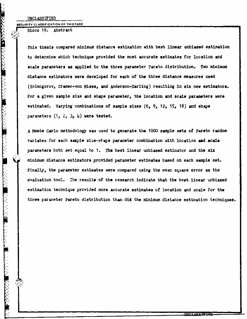
UNCLASSIFIEDSECURITY CLASSIFICATION OF THIS PAGE

J Block 19. Abstract

This thesis compared minimum distance estimation with best linear unbiased estimation

to determine which technique provided the most accurate estimates for location and

scale parameters as applied to the three parameter Pareto distribution. Two minimum

distance estimators were developed for each of the three distance measures used

(Kolmogorov, Cramer-von Mises, and Anderson-Darling) resulting in six new estimators.

For a given sample size and shape parameter, the location and scale parameters were

estimated. Varying combinations of sample sizes (6, 9, 12, 15, 18) and shape

parameters (1, 2, 3, 4) were tested.

A Monte Carlo methodology was used to generate the 1000 sample sets of Pareto random

Svariates for each vaLple size-riape parameter combination with location and scale

parameters both set equal to 1. The best linear unbiased estimator and the six

- • minimum distance estimators provided parameter estimates based on each sample set.

Finally, the parameter estimates were compared using the mean square error as the

evaluation tool. The results of the research indicate that the best linear unbiased

estimation technique provided more accurate estimates of location and scale for the

three parameter Pareto distribution than did the minimum distance estimation techniques.

'*j