A Communication Researchers' Guide to Null Hypothesis

ORIGINAL ARTICLE

A Communication Researchers’ Guide toNull Hypothesis Significance Testingand Alternatives

Timothy R. Levine1, Rene Weber2, Hee Sun Park1, & Craig R. Hullett3

1 Department of Communication, Michigan State University, East Lansing, MI 48823

2 Department of Communication, University of California, Santa Barbara, CA 93106

3 Communication, University of Arizona, Tucson, AZ 85721

This paper offers a practical guide to use null hypotheses significance testing and its

alternatives. The focus is on improving the quality of statistical inference in quantita-

tive communication research. More consistent reporting of descriptive statistics, esti-

mates of effect size, confidence intervals around effect sizes, and increasing the

statistical power of tests would lead to needed improvements over current practices.

Alternatives including confidence intervals, effect tests, equivalence tests, and meta-

analysis are discussed.

doi:10.1111/j.1468-2958.2008.00318.x

In a companion essay, Levine, Weber, Hullett, Park, and Lindsey (2008) focused on

the problems associated with null hypothesis significance testing (NHST). A com-plete ban on NHST, however, is neither tenable nor desirable. NHST is deeplyingrained in social science education, thinking, and practice and, consequently, calls

for an outright prohibition are probably unrealistic. Furthermore, as Abelson (1997)argues, there is a need to distinguish true effects from those that are explainable in

terms of mere sampling error. Although a p , .05 from a NHST does not logicallyprovide 95% or better confidence in a substantive hypothesis, a statistically signi-

ficant finding can provide some degree of evidence (Nickerson, 2000; Trafimow,2003), especially when supplemented with additional information and interpreted in

an informed and thoughtful manner.Many of the problems outlined in the companion article could be minimized

by relatively simple alterations to how NHST is used. A number of alternatives totraditional hybrid NHST are also available. Therefore, this paper explores some ofthese options. The goal here is providing applied, constructive, and concrete advice

for students, researchers, journal reviewers, and editors.

Corresponding author: Rene Weber; e-mail: [email protected]

Human Communication Research ISSN 0360-3989

188 Human Communication Research 34 (2008) 188–209 ª 2008 International Communication Association

Increased reliance on descriptive statistics

Whereas NHST and many of the alternatives and solutions discussed here involve

different applications of inferential statistics, the communication research literaturewould benefit greatly from the simple reporting of descriptive statistics. At mini-

mum, all research should report means, standard deviations, and descriptions of thedistributions for all measures. If distributions are skewed, medians, modes, or both

should be reported. Descriptive findings should always inform the substantive con-clusions drawn from data.

Rozin (2001) argues persuasively that in an effort to be more ‘‘scientific,’’ socialscientists often prematurely test hypotheses with inferential statistics, and that theorydevelopment would often be well served by preliminary descriptive work aimed at

achieving a deeper initial understanding of the topics under study. Even in researchwhere inferential statistics are needed, additional valuable information can be gained

from the reporting of central tendency, dispersion, and the shape of distributions.Examining descriptive statistics is essential for a number of reasons. Most NHST

involve assumptions about dispersion and distributions, and therefore descriptiveinformation is needed to determine if the assumptions behind inferential statistics

are met. If the distributions are highly skewed or bimodal, it may not even makesense to look at means, much less compare the means with a NHST. The reporting of

descriptive statistics is also highly valuable for subsequent meta-analysis. But, per-haps most importantly, descriptive statistics carry important substantive informa-tion that can change the interpretation of results if ignored.

For example, Burgoon, Buller, Dillman, andWalther (1995) had participants ratethe honesty of truthful and deceptive messages in an interactive deception detection

experiment. They concluded that their hypothesis that participants would ‘‘perceivedeception when it is present, was confirmed with a deception main effect on ERs’

self-reported suspicion (deception M = 3.38, truth M = 2.69), F(1, l08) = 9.31,p = .003’’ (p. 176). Arguably, however, the interpretation of these findings depends

on the scale range of the dependent measure. If 7-point scales were used, forexample, then participants in the deception condition were not especially suspi-cious, even though they were significantly more suspicious than those in the

truthful condition. This might lead to the rival conclusion that rather than peoplebeing able to detect deception, people generally believe others regardless of their

veracity, an interpretation more consistent with the results of a subsequent meta-analysis (Bond & DePaulo, 2006). Thus, a focus on p values to the exclusion of the

descriptive values can drastically alter substantive conclusions.As a second example, Levine (2001) examined differences in perceived decep-

tiveness of several types of messages. In terms of mean ratings, both lies of omissionand equivocal messages were rated as moderately deceptive and not significantly

different from each other. Examination of the distributions of ratings, however,showed that ratings of equivocal messages were normally distributed around thescale midpoint, whereas ratings of omissions were bimodal with many participants

T. R. Levine et al. Researchers’ Guide to NHST

Human Communication Research 34 (2008) 188–209 ª 2008 International Communication Association 189

rating the message as honest, whereas others rated it moderately deceptive. In thisexample, examining only the means and the t test of those means was misleading and

it masked a theoretically important difference. Simple examination of the distribu-tions was all that was needed to arrive at a more informative interpretation of the

results.In short, much valuable insight can be gained from descriptive statistics. The

current authors strongly urge researchers to report and interpret central tendency,

dispersion, and the shape of distributions along with NHSTs, effect sizes, and con-fidence intervals.

Effect sizes

Besides examining descriptive statistics, one of the easiest solutions to minimizing

the adverse consequences of many of the problems associated with NHST is to reportand interpret estimates of effect size in addition to the p values from NHST. Effectsizes are estimates of the magnitude of a difference or the strength of a statistical

association. As a general rule, it is good practice to report estimates of effect size inconjunction with all tests of statistical significance.

Reporting and interpreting effect sizes in conjunction with p values minimizesthe sensitivity to sample concern because effect size is largely independent of

sample size. Reporting effect sizes in conjunction with confidence intervals alsoprovides a solution to the null-is-always-true problem when effect tests (see below)

are not feasible. In practice, shifting focus to effect sizes requires decisions aboutwhich measure of effect size to report and assessing what a given effect size finding

means.A large number of effect size indices are available, and researchers need to

decide which estimate of effect size to report (cf. Thompson, 2007). For t tests

and ANOVA, our preference is for v2 when cell sizes are relatively small (e.g., lessthan 30) and r or h2 in studies with larger samples. h2 and r are preferred for

reasons of convention and familiarity. There is nothing wrong with reporting d, butcommunication readers are less likely to be familiar with it and, therefore, it is less

useful. There are good reasons, however, to avoid partial h2 because it is morelikely to be misleading and less useful for meta-analysis (see Hullet & Levine, 2003;

Levine & Hullett, 2002).For multiple regression analysis, questions of effect size can be more complicated.

Two major approaches to multiple regression include (a) finding a model to predict

an outcome of interest (i.e., prediction focused) and (b) examining which of thepredictors are responsible for the outcome of interest (i.e., explanation focused or

theory testing) (Pedhazur, 1997). For the first approach, effect size is more straight-forward, and the squared multiple correlation, R2, or better yet, adjusted R2, indi-

cates the amount of variance in the dependent variable accounted for by all thepredictors included in the analysis. For the second approach to multiple regression,

however, what constitutes an effect size for each predictor does not have an easy

Researchers’ Guide to NHST T. R. Levine et al.


answer. Because it is likely that the predictors are related to each other to someextent, complications such as multicollinearity and suppression can arise, and

consequently no easy solutions exist for isolating the amount of each predictor’scontribution. Commonly used and suggested measures for effect size include

standardized regression coefficients (b), partial r, semipartial r, R2change, or structure

coefficients. These, however, are not without complications or problems becauseamong many other things, they are impacted by the order in which each predictor

is entered into the model. For example, the common practice of interpreting b asanalogous to r or relying only on significance testing of b can be misleading because

b can be near zero even when the predictor explains a substantial amount of thevariance in the outcome variable when other predictors correlated with the predictor

claim the shared variance (Courville & Thompson, 2001; Thompson & Borrello,1985). Azen and Budescu (2003) provide a summary and critique of these measures

for effect size and a refinement of Budescu’s (1993) dominance analysis for evalu-ating predictor importance.

Regardless of which unit of effect size is reported, substantive interpretation

of that value is required. Rules of thumb exist, and Cohen’s (1988) labels of small(r = .10), medium (r = .30), and large (r = .50) are perhaps the most widely

known. Such rules of thumb, however, are arbitrary, and the meaning of a find-ing depends on a number of contextual considerations (cf. Thompson, 2007). For

example, the complexity of a phenomenon should be considered because themore independent causes of an outcome, the smaller the effect size for any given

predictor. Effect sizes typical of the particular literature in question might also beconsidered. For example, the median effect in social psychology research is r = .18

(Richard, Bond, & Stokes-Zoota, 2003) and the mean sex difference in commu-nication is r = .12 (Canary & Hause, 1993). In comparison, twin studies in IQresearch typically find correlations exceeding .80 for identical twins (Plomin &

Spinath, 2004). Thus, r = .30 might be a large effect in one literature, whereasr = .50 might be small in another. Finally, the pragmatic implications of the

outcome need to be considered. Consider that calcium intake and bone mass,homework and academic achievement, and the efficacy of breast cancer self-

exams are ‘‘small effects’’ on the Cohen criteria (Bushman & Anderson, 2001).Surely, one would not advocate avoiding dietary supplements, homework, and

self-exams on the basis of Cohen’s labels.When the focus is on the magnitude of an effect, there is a tendency to presume

that bigger is necessarily better and that studies reporting small effects are inherently

less valuable than studies reporting larger effect. There are, however, at least threeexceptions to the bigger is always better presumption. First, sometimes small effects

are important and small differences can have important consequences (Abelson,1985; Prentice & Miller, 1992). This can happen, for example, when predicting

infrequent events, when there is little variance in the predictor or outcome, whenthe inductions are small, or when the outcome is important but resistant to change.

Second, large effect sizes sometimes suggest validity problems such as a lack of



discriminant validity or the presence of undetected second-order unidimensionality.For example, if two measures of different constructs correlate at .80, one might

question if they are really measuring different constructs. So, effect sizes can betoo large. Finally, small effects can be informative when large effects are expected

from some accepted theory or argument but are not found in a well-conductedstudy. Convincingly, falsifying evidence can be more informative than supportiveevidence and can result in major advances in understanding.

Finally, there is sometimes confusion regarding what to make out of a large butnonsignificant effect. When the focus is shifted to effect size, there is a tendency to

presume such a large effect must be both real and substantial, and that the findingwould be statistically significant if only the sample were larger. Such thinking, how-

ever, is counterfactual. Confidence intervals, replication, or meta-analysis are neededto make sense of these findings.

In sum, although reporting and interpreting effect sizes along with p values is notsufficient to resolve all the problems with NHST, it is an easily accomplished partialsolution that ought to be encouraged. Thus, it is strongly recommended that effect

sizes be reported and interpreted in conjunction with p values for NHST. Effect sizesbecome even more useful when used in conjunction with confidence intervals.

Confidence intervals

By far, the most frequently advocated alternative to NHST is the reporting of effect

sizes with confidence intervals. Although confidence intervals can stand alone asan approach to statistical inference, they can also be used in conjunction with

NHST. Of all the inferential tools available to researchers, confidence intervals canbe among the most useful and, therefore, the use of confidence intervals is stronglyendorsed here.

Confidence intervals provide, with some specified degree of certainty, the rangewithin which a population value is likely to fall given sampling error. Confidence

intervals can be reported around descriptive statistics (e.g., means), test statistics(F, x2, t), or effect sizes. The focus here is on confidence around effect sizes, as this

is especially informative.Reporting confidence intervals around an effect size can provide all the infor-

mation contained in a NHST and more. A ‘‘statistically significant’’ result is onewhere the null hypothesis is outside the confidence interval; hence, confidence inter-vals typically provide the same information as a NHST (Natrella, 1960). In addition,

confidence intervals focus attention on effect sizes and present an upper bound inaddition to a lower bound and a precise lower bound rather than simply zero or not.

Although it is the case that confidence intervals suffer from some of the samelimitations as NHST (e.g., reliance on statistical assumptions and potential for mis-

understanding and misuse; Nickerson, 2000), a strong case can be made for themerits of confidence intervals over mere NHST and, therefore, it is reasonable to

advocate the use of confidence intervals either as an alternative or as an supplement.



Readers are referred to Cumming and Finch (2005) for a recent and accessibletreatment of confidence intervals in general.

The calculation of confidence intervals around effect sizes can be more complexthan around a pair of means. For example, the equations for determining the stand-

ard errors of regression coefficients (intercepts and slopes) vary depending uponthe measurement (e.g., continuous or categorical), transformation (e.g., centering),the number of the predictors, and so on (Aiken & West, 1991; Cohen, Cohen, West,

& Aiken, 2003). It is also the case that calculations of confidence intervals differdepending on whether random or fixed-effects designs are being used (Mendoza &

Stafford, 2001). Finally, somewhat complex procedures are required for determin-ing the confidence intervals for noncentral test distributions of t and F (e.g., for

Cohen’s d, r, or h2) when the assumption of the nil–null hypothesis is not reasonable(Cumming & Finch, 2001; Smithson, 2001). These calculations often require com-

puter patches, many of which are provided by Smithson, Bird (2002), and Fidler andThompson (2001). It is beyond the scope of this section of the paper to provide allsuch calculations here. However, a brief discussion of the calculation of confidence

intervals around r is provided below.One of the most common indices of an effect is the Pearson correlation, r, which

can be calculated directly as the measure of association between two variables orobtained through a conversion formula from an independent samples t. The stand-

ard deviation of the sampling distribution (standard error) for the populationcorrelation, r, is not useful for constructing confidence intervals around a correlation

because the sampling distribution deviates increasingly from normal as the value ofthe correlation deviates from zero (Ferguson, 1966). It is therefore suggested that the

formula sr 51 2 r2ffiffiffiffiffiffiffiffiffiN 2 1

p be avoided for anything other than with meta-analysis (Hunter& Schmidt, 1990). Instead, the nonsymmetrical nature of the confidence interval canbe obtained with Fisher’s z transformation of r(Zr). Cohen et al. (2003) present

formulas for zr and standard error and also explains the necessary calculation stepswith numeric examples on pp. 45–46 and includes a table for zr on p. 644 to help

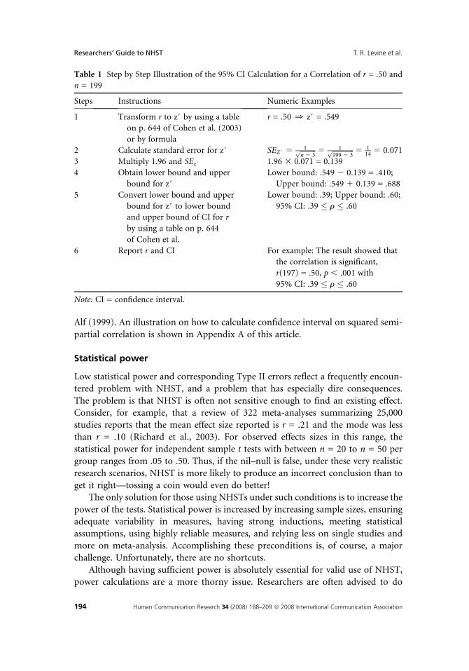
researchers to minimize computation. Tables and r-to-zr calculators were also readilyavailable online. An illustration on how to calculate confidence interval on correla-

tion is shown in Table 1.The construction of confidence intervals for the regression of a dependent vari-

able onto multiple predictors is also relatively straightforward. One can obtainstandard error of unstandardized regression coefficient, b, and confidence intervalfor each predictor, using formulas that can be found on pp. 86–87 of Cohen et al.

(2003) and from SPSS output. For confidence interval, for effect size, the formulasfor calculating standard error and confidence interval for R2 and numeric examples

can be found on p. 86 of Cohen et al. For effect size measures of each predictor,however, confidence interval construction is less straightforward. As discussed pre-

viously, some issues are involved in what constitutes an effect size in multipleregression. Nevertheless, for confidence interval on squared semipartial correlation

(or R2change), interested readers can be directed to Alf and Graf (1999) and Graf and



Alf (1999). An illustration on how to calculate confidence interval on squared semi-

partial correlation is shown in Appendix A of this article.

Statistical power

Low statistical power and corresponding Type II errors reflect a frequently encoun-tered problem with NHST, and a problem that has especially dire consequences.

The problem is that NHST is often not sensitive enough to find an existing effect.Consider, for example, that a review of 322 meta-analyses summarizing 25,000

studies reports that the mean effect size reported is r = .21 and the mode was lessthan r = .10 (Richard et al., 2003). For observed effects sizes in this range, thestatistical power for independent sample t tests with between n = 20 to n = 50 per

group ranges from .05 to .50. Thus, if the nil–null is false, under these very realisticresearch scenarios, NHST is more likely to produce an incorrect conclusion than to

get it right—tossing a coin would even do better!The only solution for those using NHSTs under such conditions is to increase the

power of the tests. Statistical power is increased by increasing sample sizes, ensuringadequate variability in measures, having strong inductions, meeting statistical

assumptions, using highly reliable measures, and relying less on single studies andmore on meta-analysis. Accomplishing these preconditions is, of course, a majorchallenge. Unfortunately, there are no shortcuts.

Although having sufficient power is absolutely essential for valid use of NHST,power calculations are a more thorny issue. Researchers are often advised to do

Table 1 Step by Step Illustration of the 95% CI Calculation for a Correlation of r = .50 and

n = 199

Steps Instructions Numeric Examples

1 Transform r to z# by using a tableon p. 644 of Cohen et al. (2003)

or by formula

r = .50 0 z# = .549

2 Calculate standard error for z# SEZ# 51ffiffiffiffiffiffiffiffiffi

n 2 3p 5 1ffiffiffiffiffiffiffiffiffiffiffiffi

199 2 3p 5 1

14 5 0:071

3 Multiply 1.96 and SEz# 1.96 3 0.071 = 0.139

4 Obtain lower bound and upper

bound for z#Lower bound: .549 2 0.139 = .410;

Upper bound: .549 1 0.139 = .688

5 Convert lower bound and upper

bound for z# to lower bound

and upper bound of CI for r

by using a table on p. 644

of Cohen et al.

Lower bound: .39; Upper bound: .60;

95% CI: .39 � r � .60

6 Report r and CI For example: The result showed that

the correlation is significant,

r(197) = .50, p , .001 with

95% CI: .39 � r � .60

Note: CI = confidence interval.



power analyses prior to data collection. To meaningfully do this, however, (a) a likelyor meaningful population effect size must be known and (b) either ideal data

(e.g., data free of measurement error and restriction in range) are required or theimpact of less than ideal data must be factored into the calculations. Absent the

former, the power analysis is arbitrary, and absent the latter, the resulting poweranalysis will be overly optimistic and misleading. Further still, if the population effectis approximately known and not zero, then the nil–null is false a priori, disproving it

is uninformative and effect significance tests (see below) rather than NHST arepreferred. That is, if enough is known about the phenomena under study to mean-

ingfully calculate power beforehand, a NHST makes less sense because the nil–null isfalse anyway. Nevertheless, so long as researchers know the magnitude of effect size

they want to be able to detect, and issues of variability and reliability are wellunderstood, power analyses are useful in planning sample size needs for data col-

lection and avoiding Type II errors.Post hoc power analyses are generally less useful than power analyses for plan-

ning purposes. Especially ill-advised are power analyses that are based upon the

effect size observed in the actual data (Hoenig & Heisey, 2001), and this type of‘‘post hoc’’ or ‘‘observed power’’ analysis should typically be avoided, even though

it is an option on SPSS output. One reason is that the post hoc, observed power,and the observed p value from a NHST are completely redundant. Nonsignificant

results, by definition, lack observed power. Only ‘‘after the fact’’ power analyses thatare based on projected population effect sizes of independent interest are poten-

tially meaningful (O’Keefe, in press). So, journal editorial policies that instructauthors to report ‘‘power estimates when results are nonsignificant’’ might specify

that reported power be based not on observed effects but on what is a meaningfuleffect in the given research context. Finally, power analyses absolutely should not beused as evidence for accepting the nil–null. A nonsignificant result for a traditional

NHST cannot be interpreted as supporting a nil–null even if the power to detectsome nonzero effect is high. Arguments for a null require ranged null hypotheses

and equivalence tests (see below).

Effect testing

Effect testing is a useful alternative to nil–NHST when the anticipated effects canbe more precisely articulated. In effect testing, like NHST, the null hypotheses istested and rejected or not based on the probability of the data under the null.

But, unlike standard two-tailed NHST, the null is no longer a point null but insteadcovers a range of values. Different from standard one-tailed NHST, the upper

bound of the null is not zero. Thus, the primary conceptual difference betweeneffect testing and standard NSHT is more flexibility in the construction of the

null hypothesis.One of the problems with the typical NHST approach is that the standard

nil–null hypothesis is almost always literally false. Testing a pure ‘‘sign hypothesis’’



(H0: effect � 0; H1: effect . 0, i.e., an effect is either positive or negative) withstandard nil–NHST is neither risky nor informative for more advanced theoretical

reasoning in communication research. Researchers may want more than just notzero. As an alternative to nil–null hypotheses, researchers could use null hypotheses

reflecting reasonable assumptions about an effect that would count as a trivial effect.This is the rationale for effect testing.

D in effect testing is defined as an effect that is considered inconsequential on the

basis of substantive theoretical and practical considerations. In other words, D isdefined as the maximum effect that is still considered as ‘‘no effect’’ (maximum no

effect). D reflects the bounds of the null hypothesis and any effect that is ‘‘significant’’needs to be greater than D at p, .05. Thus, for a positive effect, the one-tailed effect

test specifies a null hypothesis of H0: effect � D (H1: effect . D) instead of just H0:effect � 0 as in nil–NHST.

Statistically, D can be depicted as a Pearson correlation and can be understood asa universal population effect size measure (Cohen, 1988) to which other effect sizemeasures (e.g., standardized mean differences) can be converted. Provided that

researchers are able to meaningfully define D, many of the nil–NHST problems,including the problem that the null is never literally true, can be avoided

(cf. Klemmert, 2004). Those effect tests are riskier because stronger effects, bettertheories, and, ultimately, better data are needed to reject effect-null hypotheses.

Adopting effect tests over nil–NHST challenges communication scholars to definebetter models and to build better theories because researchers are forced to define

which effect sizes are of interest and which are not.As an example, consider an experiment recently published inHCR examining the

impact of argument quality on attitude change (Park, Levine, Kingsley Westerman,Orfgen, & Foregger, 2007). Park et al. exposed n1 = 335 research participants tostrong arguments and n2 = 347 to weak arguments. A meta-analysis also reported in

Park et al. showed that previous research found that strong arguments are morepersuasive than weak arguments and this effect can be quantified with a Pearson

correlation of r = .34.In order to conduct an effect test on the Park et al. (2007) data, the key ques-

tion is what qualifies as the maximum no effect (D) in this research. Note that Ddefines a maximum no effect (i.e., D belongs to the effect-null hypothesis) and

not a minimum substantive effect. That is, D defines the null hypothesis not thealternative hypothesis; it is a value that can be rejected if p , .05. Deciding whatqualifies as the maximum no effect (D) is probably the most difficult question

involved in effect testing and significance testing in general. Murphy and Myors(1999) suggest using an average effect found in meta-analyses, converting this

effect to an explained variance, and use half of the explained variance as orienta-tion for a maximum no effect. With r = .34 in this example’s meta-analysis, the

explained variance is r2 = .1156. This divided by 2 results in an explained varianceof r2 = .0587. The square root of this result then defines themaximum no effect, which

is D = .24.



Because our example uses rating scales and compares two means (mean attitudechange of weak arguments m1 vs. strong arguments m2), the standardized mean

difference d is used here, which is defined as:

d 5m1 2 m2

s

s is the standard deviation of attitude change (dependent variable). The standard-ized mean difference d can easily be converted to the correlation measure D and vice

versa using the following formulas (cf. Cohen, 1988; Kraemer & Thiemann, 1987):

D 5 1:25dffiffiffiffiffiffiffiffiffiffiffiffiffiffiffiffiffiffiffiffiffiffiffiffi

d2 1 1=ðpqÞp

p 5n1n

q 5n2n

n1 1 n2 5 n

d 5

ffiffiffiffiffiffiffiffiffiffiffiffiffiffiffiffiffiffiffiffiffiffiD2=pq

1:252 2 D2

r

Thus, D = .24 in the example corresponds to a standardized mean difference ofd = 0.39 (n1 = 335, n2 = 347).

For this demonstration, we follow first Murphy and Myor’s (1999) recommen-dation and use D = .24 or d = 0.39 as the maximum no effect. Thus, our effect test

hypotheses in this example are:

H0 :m1 2 m2

s� 0:39 H1 :

m1 2 m2

s. 0:39

Identical to nil–NHST, effect tests calculate the probability of empirical results thatare equal or more distant from the H0 parameter (in direction to the H1 parameter)

on condition that the null hypothesis sampling distribution is true. In nil–NHST, thenull hypothesis sampling distribution for a standardized mean difference is a central

t distribution with n1 1 n2 2 2 degrees of freedom. In effect–NHST, however, thisdistribution is replaced by a noncentral t distribution with n1 1 n2 2 2 degrees offreedom and a noncentrality parameter l that can easily be calculated according to

the following formula (d is the above defined maximum no effect of .39; n1 and n2are the sample sizes):

l 5 d

ffiffiffiffiffiffiffiffiffiffiffiffiffiffiffiffin1n2

n1 1 n2

r

Using a noncentral test distribution basically means that for l . 0 (positive effects),

the test distribution is skewed to the right and for l, 0 (negative effects) skewed tothe left (Cumming & Finch, 2001).



Similar to nil–NHST, effect–NHST (for positive effects; one-tailed test) rejectsthe null hypothesis if:

temp . tcritð1 2 a; n1 1 n2 2 2; lÞ

temp 5�x1 2 �x2

s


n1 1 n2

r

The empirical t value corresponds to the standard two independent groups t test thattests a nil–null hypothesis and can be read off a standard SPSS output (s is the sample

standard deviation of attitude change). In the Park et al. (2007) study, the empiricalt value of a standard two independent samples t test is 8.2, n1 = 335 (strong argument),n2 = 347 (weak argument), and thus, l(d = 0.39) = 5.09.

Unfortunately, effect tests and noncentral test distributions are not part of themenu options in standard statistical software packages such as SPSS. Nevertheless,

p values that are based on noncentral distributions can be calculated with SPSS andother statistical software. To do so, one first needs to create a new data file that

contains only one case with the values of the following four variables: (a) empirical tvalue (read off a standard t-test table in SPSS based on the same data, variable name

is t); (b) n1 (sample size in group 1, weak argument, variable name is n1); (c) n2(sample size in group 2, strong argument, variable name is n2); and (d) d (.39 in thisexample, variable name is delta). The following SPSS syntax commands calculate the

parameter l and the p value of an effect test (positive effect; one-tailed test).

Table 2 contains p values for different D and d, including d = 0.39 for thisexample. As one can see, the results indicate a substantial impact of argument quality

on attitude change assuming that effects smaller than D = .24 or d = 0.39 indicateno effect. The interpretation of data for the present example is that the observed

Table 2 D, d, and p Values of a Noncentral t Distribution (temp = 8.2, n1 = 335, n2 = 347)

Associated with Park et al. (2007)

D (Max No Effect) d (Max No Effect) p Value

.10 0.16 , .0001

.24 0.39 .0012

.30 0.50 .0446

.34 0.57 .6111

.50 0.87 .9991



standardized mean difference is greater than the maximum no effect value d = 0.39(or the effect size expressed as a correlation of D = .24) and that difference is very

unlikely due to chance (p , .0,012).Similar to this example, one can create effect tests that involve dependent sam-

ples, more than two means, bivariate and multiple correlations, negative effects, andtwo-tailed tests (cf. Klemmert, 2004; Weber, Levine, & Klemmert, 2007). Thus, effecttesting is flexible and can be used in a variety of situations where researchers want

a test more stringent than a nil–null test.There are alternative strategies to defining a maximum no effect. Klemmert

(2004) proposes conservative, balanced, and optimistic strategies. In the conservativestrategy, the maximum no effect equals an average substantial effect found in meta-

analyses. Thus, D would be assumed as .34 as indicated by the meta-analysis in ourexample. In an optimistic strategy, Klemmert and also Fowler (1985) recommend

using Cohen’s (1988) effect sizes categorization, which suggests using D = .10 ord = 0.16 (small effect) as a maximum no effect. In a balanced strategy, the maximumno effect would be assumed as the middle course of the conservative and optimistic

strategy, thus D would be assumed as the mean of .34 and .10, which is .22 and closeto D = .24 as suggested by Murphy and Myors (1999) and used above.

Thus, applied to our example, if the conservative strategy is applied to the Parket al. (2007) data, the result would be nonsignificant. This means that the observed

effect in the Park et al. study is not statistically greater than the average effect foundin other studies (D = .34, the average effect in the meta-analysis) and would be

considered as no effect. However, as shown in Table 2, the Park et al. results arestatistically significant when using either the balanced or the optimistic strategies.

Table 2 also provides p values for D = .10 (small effect), D = .30 (medium effect), andD = .50 (large effect) as maximum no effect as well.

There are at least two reasons why effect testing, as an alternative to classical

nil–NHST, is seldom if ever used in communication research. First, the concept ofeffect-null hypotheses and its theoretical background may be unfamiliar to many

communication scholars (and other quantitative social scientists) because unfortu-nately it is not part of the typical statistical training. Second, effect-null hypothesis tests

require noncentral sampling distributions that are often not available as preprog-rammed statistical procedures in most standard statistical software packages (such as

SPSS, SAS, STATISTICA). Klemmert (2004) andWeber et al. (2007), however, providea description of various risky effect tests and also equivalence tests (for mean differ-ences, correlations, etc.), including simulations of test characteristics and relatively

simple programs for standard statistical software. Therefore, effect–NHST will hope-fully be usedmore frequently in social scientific communication research in the future.

Equivalence testing

Equivalence tests are inferential statistics designed to provide evidence for a null

hypothesis. Like effect tests, the nil–null is eschewed in equivalence testing. However,



unlike both standard NHST and effect tests, equivalence tests provide evidence thatthere is little difference or effect. A significant result in an equivalence test means that

the hypothesis that the effects or differences are substantial can be rejected. Hence,equivalence tests are appropriate when researchers want to show little difference

or effect.It is well known that NHST does not provide a valid test of the existence of ‘‘no

effect’’ or the equivalence of two effects. That is, with NHST, a nonsignificant

result does not provide evidence for the null. We either reject or fail to reject thenull. It is never accepted. As a consequence, current researchers likely have few

known options when the null hypothesis is the desired hypothesis. For instance,media scholars may be interested in showing that exposure compared with non-

exposure to violent messages does not translate into different levels of aggressivebehavior (cf. Ferguson, in press). Examples that are more common include testing

the assumption of statistical tests that population variances are homogeneous,testing fit in structural equation models, and testing effect homogeneity in meta-analysis. Although most researchers know that a nonsignificant result under the

assumption of a nil–null hypothesis cannot be used as good evidence for equiva-lence, nonsignificant results are nevertheless interpreted as equivalence with an

unfortunately high frequency.Although equivalence tests do not provide a solution for classical NHST, they

offer a correct alternative for NHST when the goal of a test or a study is to demon-strate evidence for a null hypothesis rather than for a research hypothesis. Equiva-

lence tests are the logical counterpart of effect tests and the basic analytical logic is thesame. The null hypothesis of an effect test (positive effect, one-tailed test) is specified

by H0: effect � D (H1: effect. D, see above) and D has been defined asmaximum noeffect. The null hypothesis of an equivalence test is H0: effect � D (H1: effect , D).The difference is that D in equivalence tests is defined as minimum substantial effect.

A significant result in an equivalence test provides evidence that an effect is signi-ficantly smaller than D and, therefore, is considered as functionally equivalent.

To simplify, in NHST, the null hypothesis always defines the conditions that wewant to disprove. So, while null hypotheses in effect tests try to exclude effects that

are too small or in the wrong direction, null hypotheses in equivalence tests try toexclude too-large effects.

As an example, consider a media communication scholar who wants to findevidence that playing violent video games is not linked to increased aggressivethoughts in players. In an experiment, the researcher assigns n = 251 research

participants randomly to two versions of a game—one version with violent content(n1 = 127) and another version with all violent content replaced with nonviolent

content (n2 = 124). The number of aggressive thoughts in a story completion taskserves as the dependent variable. From a recent meta-analyses (cf. Ferguson, in

press), the average correlation between exposure to violence in video games andaggressive thoughts is assumed to be r = .25. Because this average correlation has

been found and documented in many independent studies, our researcher uses this



information as a minimum substantial effect of D = .25, which corresponds toa standardized mean difference (n1 = 127, n2 = 124) of d = .41. The question, then,

is: If D = .25 or d = .41 is considered as minimum substantial effect, is the effect thatthe researcher found in his/her study small enough then to count as evidence for

equivalence? Hence, the hypotheses for this equivalence test example are:

H0 :m1 2 m2

s� 0:41 H1 :

m1 2 m2

s, 0:41

This equivalence test (for positive effects; one-tailed test) rejects the null hypothesis if:

temp,tcritða; n1 1 n2 2 2; lÞ

temp 5�x1 2 �x2

s


n1 1 n2

r

Again, the empirical t value corresponds to the one of a standard two indepen-

dent sample t test that tests a nil–null hypothesis and can be read off a standardSPSS output (s is the sample standard deviation of the number of aggressivethoughts). In our example, the found sample means are �x1 5 4:124 and�x2 5 3:955 and the empirical t value in the SPSS standard output is temp = 1.26(n1 = 127, n2 = 124). With d = .41, l equals 3.25 (see formula in section ‘‘Effect

testing’’). The SPSS file and the SPSS commands that are needed to calculate theequivalence test’s (one-tailed test; positive effect) p value are identical to the ones

for the effect test (see above) with one exception: The command line ‘‘COMPUTEp = 1 2 NCDF.T (t, df, lambda)’’ for the calculation of p value in a noncentral

t distribution has to be replaced with ‘‘COMPUTE p = NCDF.T(t, df, lambda).’’The p value of the found result in this equivalence test is p , .023. Hence, theempirically observed standardized mean difference in this study is significantly

smaller than a minimum substantial effect of d = 0.41 and is very unlikely due tochance (p , .023).

Note that a nonsignificant equivalence test result does not provide evidence foreither the null or the alternative. Just as a nonsignificant NHST does not mean that

the null is accepted, a nonsignificant equivalence test does not provide evidence thatthe effect is substantial. A nonsignificant equivalence tests means that a substantial

effect is not ruled out.The reasons why correctly conducted equivalence tests are rarely used in

communication research (in contrast to other research fields such as pharmaceu-tical research) are likely the same as for effect tests. Hopefully, though, as com-munication researchers become aware of equivalence tests as an option, they will

use them when needed. For a more detailed discussion of equivalence tests,including equivalence tests for the most relevant test variants in communication

research and their correct execution with standard statistical software, see Weberet al. (2007).



Meta-analysis

Meta-analysis involves cumulating effects across studies. Findings from all the stud-

ies testing a hypothesis are converted to the same metric with a conversion formula,the effects are averaged, and the dispersion of effects is examined. Although

meta-analysis can never replace original research (meta-analysis cannot be doneabsent original research to analyze), meta-analysis does offer a solution to many

of the problems created by NHST. Therefore, less reliance on NHST in individualstudies and a greater reliance on quantitative summaries of across-study data

(Schmidt & Hunter, 1997) are recommended.Meta-analysis is especially useful at overcoming the power and Type II error

problems. Because effects are summed across studies, meta-analyses deal with larger

sample sizes than individual studies and consequently offer greater statistical powerand more precise confidence intervals. Meta-analysis, too, like confidence intervals,

focuses attention on effect size rather than just the p value.Meta-analysis also helps overcome another problem with NHST that was not

explicitly discussed in the companion paper. Absent meta-analysis, confidenceintervals, or both, the reliance on NHST makes integrated, across-study conclusions

within research literatures difficult if not impossible.Low power and methodological artifacts that attenuate effect sizes guarantee that

some large proportion of tests of any viable substantive hypotheses will be nonsigni-ficant (Meehl, 1986; Schmidt &Hunter, 1997). Schmidt and Hunter estimate that 50%or more of NHSTs result in false negative findings. Alternatively, infrequent Type I

errors, systematic error due to confounds and spurious effects, and a publication biasfavoring statistically significant results can produce significant findings supporting

erroneous substantive hypotheses (Meehl, 1986). Meehl demonstrates how 70% ofpublished tests of a false substantive hypothesis could be statistically significant. The

net result is that virtually all quantitative social science literatures contain a confusingcollection of significant and nonsignificant results, and raw counts (or proportions) of

statistically significant findings are uninformative (Meehl, 1986). The media violenceliterature may be a good example of this point. Well-conducted meta-analyses offera solution by summarizing effects across a literature, assessing variability that might be

due to sampling error and artifact, addressing publication biases by conducting fail-safe N analyses (Carson, Schriesheim, & Kinicki, 1990; Rosenthal, 1979), and system-

atically looking for identifiable moderators.A potential but avoidable limitation in meta-analysis is that NHST can be

misused and misunderstood within meta-analyses just as it can in single studies.For example, NHST is often used to test the across-study average effect against the

nil–null and to assess homogeneity of effects as an indicator of the presence ofmoderators. Although low statistical power is less of a problem in the former use,

NHSTs should be replaced by (a) risky effect significance tests (see above) to dem-onstrate a substantial significant effect, (b) equivalence tests (see above) to assesshomogeneity of effects, and c) confidence intervals around average effect estimates.



Summary and conclusion

Severe problems with standard NHST exist (Levine et al., 2008). Fortunately, the

negative impact of many of the problems associated with standard NHST can beminimized by simple changes in how NHST are used and interpreted. Supplement-

ing the information provided by NHST with information for descriptive statistics,effect sizes, and confidence intervals is strongly advised. Furthermore, several viable

alternatives to NHST also exist. These include confidence intervals, using effect orequivalence testing instead of testing standard nil–null hypotheses, increased reliance

on descriptive statistics, and meta-analysis. Moreover, NHST and its alternativesneed not be mutually exclusive options. The quality of the inference gained froma standard NHST are greatly improved when coupled with the thoughtful examina-

tion of descriptive statistics and effect sizes with confidence intervals.Simple awareness of the inferential challenges posed by NHST and more

informed interpretation of findings can overcome problems associated with mis-understanding and abuse. Using NHST mindlessly to make dichotomous support–

reject inferences about substantive hypotheses should be avoided. Ensuring sufficientstatistical power, interpreting results in light of observed effect sizes (or better defin-

ing effect-null hypotheses rather than nil–null hypotheses), confidence intervals,descriptive statistics, and using NHST along with sound research design and mea-

surement would substantially improve the quality of statistical inference. Replicationprovides a guard against Type I errors and meta-analyses guards against Type IIerrors. More sophisticated researchers should make use of effect tests and equiva-

lence tests.None of these solutions is perfect and none are universally applicable. All are

subject to misunderstanding and abuse. Nevertheless, more accurate and informedreporting and interpretation, a wider repertoire of data analysis strategies, and rec-

ognition that these options are not mutually exclusive are advocated.

References

Abelson, R. P. (1985). A variance explanation paradox: When little is a lot. Psychological

Bulletin, 97, 129–133.

Abelson, R. P. (1997). A retrospective on the significance test ban of 1999 (if there were no

significance tests, they would be invented). In L. L. Harlow, S. A. Mulaik, & J. H. Steiger

(Eds.), What if there were no significance tests? (pp. 117–141). Mahwah, NJ: LEA.

Aiken, L. S., & West, S. G. (1991). Multiple regression: Testing and interpreting interactions.

Newbury Park, CA: Sage.

Alf, E. F. Jr., & Graf, R. G. (1999). Asymptotic confidence limits for the difference between two

squared multiple correlations: A simplified approach. Psychological Methods, 4, 70–75.

Azen, R., & Budescu, D. V. (2003). The dominance analysis approach for comparing

predictors in multiple regression. Psychological Methods, 8, 129–148.

Bird, K. (2002). Confidence intervals for effect sizes in analysis of variance. Educational and

Psychological Measurement, 62, 197–226.



Bond, C. F. Jr., & DePaulo, B. M. (2006). Accuracy of deception judgments. Review of

Personality and Social Psychology, 10, 214–234.

Budescu, D. V. (1993). Dominance analysis: A new approach to the problem of relative

importance of predictors in multiple regression. Psychological Bulletin, 114, 542–551.

Burgoon, J. K., Buller, D. B., Dillman, L., & Walther, J. B. (1995). Interpersonal deception IV.

Effects of suspicion on perceived communication and nonverbal behavior dynamics.

Human Communication Research, 22, 163–196.

Bushman, B. J., & Anderson, C. A. (2001). Media violence and the American public.

American Psychologist, 56, 477–489.

Canary, D. J., & Hause, K. S. (1993). Is there any reason to research sex differences in

communication? Communication Quarterly, 41, 129–144.

Carson, K. P., Schriesheim, C. A., & Kinicki, A. J. (1990). The usefulness of the ‘‘fail-safe’’

statistic in meta-analysis. Educational and Psychological Measurement, 50, 233–243.

Cohen, J. (1988). Statistical power analysis for the behavioral sciences (2nd ed.). Hillsdale,

NJ: LEA.

Cohen, J., Cohen, P., West, S. G., & Aiken, L. S. (2003). Applied multiple regression/correlation

analysis for the behavioral sciences (3rd ed.). Mahwah, NJ: LEA.

Courville, T., & Thompson, B. (2001). Use of structure coefficients in published multiple

regression articles: B is not enough. Educational and Psychological Measurement, 61,

229–248.

Cumming, G., & Finch, S. (2001). A primer on the understanding, use, and calculation of

confidence intervals that are based on central and noncentral distributions. Educational

and Psychological Measurement, 61, 532–574.

Cumming, G., & Finch, S. (2005). Confidence intervals and how to read pictures of data.

American Psychologist, 60, 170–180.

Ferguson, C. J. (2007). Evidence for publication bias in video game violence effects literature:

A meta-analytic review. Aggression and Violent Behavior, 12, 470–482.

Ferguson, G. A. (1966). Statistical analysis in psychology and education. New York:

McGraw-Hill.

Fidler, F., & Thompson, B. (2001). Computing confidence intervals for ANOVA fixed-

and random-effects effect sizes. Educational and Psychological Measurement, 61,

575–604.

Fowler, R. L. (1985). Testing for substantive significance in applied research by specifying

nonzero effect null hypotheses. Journal of Applied Psychology, 70, 215–218.

Graf, R. G., & Alf, E. F. Jr. (1999). Correlations redux: Asymptotic confidence limits for

partial and squared multiple correlations. Applied Psychological Measurement, 23,

116–119.

Hoenig, J. M., & Heisey, D. M. (2001). The abuse of power: The pervasive fallacy of power

calculations for data analysis. American Statistician, 55, 19–24.

Hullet, C. R., & Levine, T. R. (2003). The overestimation of effect sizes from F values in

meta-analysis: The cause and a solution. Communication Monographs, 70, 52–67.

Hunter, J. E., & Schmidt, F. L. (1990). Methods of meta-analysis: Correcting error and bias in

research findings. Newbury Park, CA: Sage.

Klemmert, H. (2004). Aquivalenz- und Effekttests in der psychologischen Forschung.

[Equivalence and effect tests in psychological research]. Frankfurt/Main, Germany:

Peter Lang.



Kraemer, H. C., & Thiemann, S. (1987). How many subjects? Statistical power analysis in

research. Beverly Hills, CA: Sage.

Levine, T. R. (2001). Dichotomous and continuous views of deception: A reexamination of

deception ratings in information manipulation theory. Communication Research Reports,

18, 230–240.

Levine, T. R., & Hullett, C. (2002). Eta-square, partial eta-square, and misreporting of effect

size in communication research. Human Communication Research, 28, 612–625.

Levine, T. R., Weber, R., Hullett, C. R., Park, H. S., & Lindsey, L. (2008). A critical assessment

of null hypothesis significance testing in quantitative communication research. Human

Communication Research, 34, 171–187.

Meehl, P. E. (1986). What social scientists don’t understand. In D. W. Fiske & R. A. Shweder

(Eds.), Meta-theory in social science (pp. 315–338). Chicago: University of Chicago Press.

Mendoza, J. L., & Stafford, K. L. (2001). Confidence intervals, power calculation, and sample

size estimation for the squared multiple correlation coefficient under the fixed and

random regression models: A computer program and useful standard tables. Educational

and Psychological Measurement, 61, 650–667.

Murphy, K. R., & Myors, B. (1999). Testing the hypothesis that treatments have negligible

effects: Minimum-effect tests in the general linear model. Journal of Applied Psychology,

84, 234–248.

Natrella, M. G. (1960). The relation between confidence intervals and tests of significance—A

teaching aid. American Statistician, 14, 20–38.

Nickerson, R. S. (2000). Null hypothesis significance testing: A review of an old and

continuing controversy. Psychological Methods, 5, 241–301.

O’Keefe, D. J. (in press). Post hoc power, observed power, a priori power, retrospective

power, prospective power, achieved power: Sorting out appropriate uses of statistical

power analyses. Communication Methods and Measures.

Park, H. S., Levine, T. R., Kingsley Westerman, C. Y., Orfgen, T., & Foregger, S. (2007). The

effects of argument quality and involvement type on attitude formation and attitude

change: A test of dual-process and social judgment predictions. Human Communication

Research, 33, 81–102.

Pedhazur, E. J. (1997). Multiple regression in behavioral research (3rd ed.). Forth Worth,

TX: Harcourt.

Plomin, R., & Spinath, F. M. (2004). Intelligence: Genetics, genes, and genomics. Journal of

Personality and Social Psychology, 86, 112–129.

Prentice, D. A., & Miller, D. T. (1992). When small effects are impressive. Psychological

Bulletin, 112, 160–164.

Richard, F. D., Bond, C. F., & Stokes-Zoota, J. J. (2003). One hundred years of social

psychology quantitatively described. Review of General Psychology, 7, 331–363.

Rosenthal, R. (1979). The ‘‘file drawer problem’’ and tolerance for null results. Psychological

Bulletin, 86, 638–641.

Rozin, P. (2001). Social psychology and science: Some lessons from Solomon Asch.

Personality and Social Psychology Review, 5, 2–14.

Schmidt, F. L., & Hunter, J. E. (1997). Eight common but false objections to the

discontinuation of significance testing in the analysis of research data. In L. L. Harlow,

S. A. Mulaik, & J. H. Steiger (Eds.), What if there were no significance tests? (pp. 37–64).

Mahwah, NJ: LEA.



Smithson, M. (2001). Correct confidence intervals for various regression effect sizes and

parameters: The importance of noncentral distributions in computing intervals.

Educational and Psychological Measurement, 61, 605–632.

Thompson, B. (2007). Effect sizes, confidence intervals, and confidence intervals for effect

sizes. Psychology in the Schools, 44, 423–432.

Thompson, B., & Borrello, G. M. (1985). The importance of structure coefficients in

regression research. Educational and Psychological Measurement, 45, 203–209.

Trafimow, D. (2003). Hypothesis testing and theory evaluation at the boundaries: Surprising

insights from Bayes’s theorem. Psychological Review, 110, 526–535.

Weber, R., Levine, T. R., & Klemmert, H. (2007). Testing equivalence in communication

research. Manuscript submitted for publication.

Appendix A

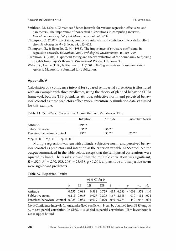
Calculation of a confidence interval for squared semipartial correlation is illustrated

with an example with three predictors, using the theory of planned behavior (TPB)framework because TPB postulates attitude, subjective norm, and perceived behav-

ioral control as three predictors of behavioral intention. A simulation data set is usedfor this example.

Table A1 Zero-Order Correlations Among the Four Variables of TPB

Intention Attitude Subjective Norm

Attitude .49***

Subjective norm .33*** .36***

Perceived behavioral control .23** .33*** .26***

***p , .001. **p , .01. *p , .05.

Multiple regression was run with attitude, subjective norm, and perceived behav-ioral control as predictors and intention as the criterion variable. SPSS produced the

output summarized in the table below, except that the semipartial correlations weresquared by hand. The results showed that the multiple correlation was significant,

R = .520, R2 = .270, F(3, 206) = 25.458, p , .001, and attitude and subjective normwere significant predictors.

Table A2 Regression Results

b SE

95% CI for b

b t p rsp r2spLB UB

Attitude 0.555 0.088 0.381 0.729 .415 6.283 ,.001 .374 .140

Subjective norm 0.115 0.045 0.027 0.203 .167 2.588 .010 .154 .024

Perceived behavioral control 0.025 0.033 20.039 0.090 .049 0.774 .440 .046 .002

Note: Confidence intervals for unstandardized coefficient, b, can be obtained from SPSS output;

rsp = semipartial correlation. In SPSS, it is labeled as partial correlation. LB = lower bound;

UB = upper bound.



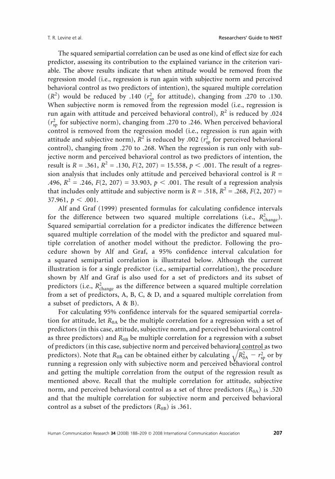
The squared semipartial correlation can be used as one kind of effect size for eachpredictor, assessing its contribution to the explained variance in the criterion vari-

able. The above results indicate that when attitude would be removed from theregression model (i.e., regression is run again with subjective norm and perceived

behavioral control as two predictors of intention), the squared multiple correlation(R2) would be reduced by .140 (r2sp for attitude), changing from .270 to .130.When subjective norm is removed from the regression model (i.e., regression is

run again with attitude and perceived behavioral control), R2 is reduced by .024(r2sp for subjective norm), changing from .270 to .246. When perceived behavioral

control is removed from the regression model (i.e., regression is run again withattitude and subjective norm), R2 is reduced by .002 (r2sp for perceived behavioral

control), changing from .270 to .268. When the regression is run only with sub-jective norm and perceived behavioral control as two predictors of intention, the

result is R = .361, R2 = .130, F(2, 207) = 15.558, p , .001. The result of a regres-sion analysis that includes only attitude and perceived behavioral control is R =.496, R2 = .246, F(2, 207) = 33.903, p , .001. The result of a regression analysis

that includes only attitude and subjective norm is R = .518, R2 = .268, F(2, 207) =37.961, p , .001.

Alf and Graf (1999) presented formulas for calculating confidence intervalsfor the difference between two squared multiple correlations (i.e., R2

change).

Squared semipartial correlation for a predictor indicates the difference betweensquared multiple correlation of the model with the predictor and squared mul-

tiple correlation of another model without the predictor. Following the pro-cedure shown by Alf and Graf, a 95% confidence interval calculation for

a squared semipartial correlation is illustrated below. Although the currentillustration is for a single predictor (i.e., semipartial correlation), the procedureshown by Alf and Graf is also used for a set of predictors and its subset of

predictors (i.e., R2change as the difference between a squared multiple correlation

from a set of predictors, A, B, C, & D, and a squared multiple correlation from

a subset of predictors, A & B).For calculating 95% confidence intervals for the squared semipartial correla-

tion for attitude, let R0A be the multiple correlation for a regression with a set ofpredictors (in this case, attitude, subjective norm, and perceived behavioral control

as three predictors) and R0B be multiple correlation for a regression with a subsetof predictors (in this case, subjective norm and perceived behavioral control as twopredictors). Note that R0B can be obtained either by calculating

ffiffiffiffiffiffiffiffiffiffiffiffiffiffiffiffiffiffiffiR20A 2 r2sp

qor by

running a regression only with subjective norm and perceived behavioral controland getting the multiple correlation from the output of the regression result as

mentioned above. Recall that the multiple correlation for attitude, subjectivenorm, and perceived behavioral control as a set of three predictors (R0A) is .520

and that the multiple correlation for subjective norm and perceived behavioralcontrol as a subset of the predictors (R0B) is .361.



R0B 5

ffiffiffiffiffiffiffiffiffiffiffiffiffiffiffiffiffiffiffiR20A 2 r2sp

q5

ffiffiffiffiffiffiffiffiffiffiffiffiffiffiffiffiffiffiffiffiffiffiffiffi:270 2 :140

p5

ffiffiffiffiffiffiffiffiffi:130

p5 :361

Let RAB be correlation between the full set of predictors (attitude, subjective norm,and perceived behavioral control) and the subset of predictors (subjective norm andperceived behavioral control). A formula for RAB simplified by Alf and Graf (1999)

and its calculation for this data set are shown below.

RAB 5R0B

R0A5

:361

:5205 :694

R2AB 5 :482

The variance of the difference between the multiple correlation for attitude, sub-

jective norm, and perceived behavioral control as a set of three predictors (R0A), andthe multiple correlation for subjective norm and perceived behavioral control asa subset of the predictors (R0B) is shown below.

varNðR20A 2 R2

0BÞ 54R2

0Að1 2 R20AÞ2

n1

4R20Bð1 2 R2

0BÞ2n

28R0AR0B½0:5ð2RAB 2 R0AR0BÞð1 2 R2

0A 2 R20B 2 R2

ABÞ 1 R3AB�

n

54 3 :270ð1 2 :270Þ2

2101

4 3 :130ð1 2 :130Þ2210

283 :5203 :361½0:5½ð23 :694Þ2ð:5203 :361Þ�ð12 :2702 :1302 :482Þ1ð:694Þ3�

210

5 0:0027 1 0:0019 2 0:0029 5 0:0017

Finally, calculation of the 95% confidence interval is shown below.

95% confidence limits 5 ðR20A 2 R2

0BÞ � 1:96ffiffiffiffiffiffiffiffiffiffiffiffiffiffiffiffiffiffiffiffiffiffiffiffiffiffiffiffiffiffiffiffiffiffivarNðR2

0A 2 R20BÞ

q

5 r2sp � 1:96ffiffiffiffiffiffiffiffiffiffiffiffiffiffiffiffiffiffiffiffiffiffiffiffiffiffiffiffiffiffiffiffiffiffivarNðR2

0A 2 R20BÞ

q

5 :140� 1:96ffiffiffiffiffiffiffiffiffiffiffiffiffi0:0017

p5 :140� 0:081

Thus, for the squared semipartial correlation for attitude, the 95% confidence inter-val is .059� r2sp� .221.

For calculating 95% confidence intervals for the squared semipartial correlationsof subjective norm and of perceived behavioral control, the above formula and the

same calculation procedure can be used. However, although not shown here, thecalculation of confidence intervals for squared semipartial correlations of subjectivenorm and of perceived behavioral control yielded the lower limit of its 95% confi-

dence interval to be below the value of zero, even when a predictor has a statistically



significant regression coefficient (i.e., the result showed that subjective norm wasa statistically significant predictor and had a small squared semiparital correlation).

Researchers may encounter similar phenomena with their data. Normally, a valuebelow zero is a mathematically impossible number because ‘‘in any sample, the

multiple correlation between a criterion and a full set of predictors can never be lessthan the multiple correlation between that criterion and a subject of those predic-tors’’ (Alf & Graf, 1999, p. 74). Nevertheless, numerically it can happen and should

not result in concluding no statistical significance for that predictor because thestatistical testing provided by SPSS is not for a squared semipartial correlation but

for a regression coefficient. If the difference between R0B and R0A (i.e., R2change) is not

significant according to an F test and/or very small, ‘‘then the approximation for this

case will be inappropriate, regardless of sample size . it is not possible to use theseapproximation methods to make a significant test’’ (Graf & Alf, 1999, p. 118).

Therefore, caution should be exercised for confidence intervals for statistically insig-nificant R2

change and/or very small square semipartial correlations.



Le guide du test de signification basé sur l’hypothèse nulle et de ses alternatives, à

l’usage des chercheurs en communication

Timothy R. Levine

Michigan State University

René Weber

University of California Santa Barbara

Hee Sun Park


Craig R. Hullett

University of Arizona

Résumé

Cet article offre un guide pratique pour l’utilisation du test de signification basé sur

l’hypothèse nulle (NHST) et de ses alternatives. Il se concentre sur la manière

d’améliorer la qualité de l’inférence statistique dans la recherche quantitative en

communication. Une divulgation plus cohérente de la statistique descriptive, une

évaluation de l’ampleur de l’effet, des intervalles de confiance autour de l’ampleur de

l’effet et une augmentation de l’efficacité statistique des tests mèneraient à de nécessaires

améliorations des pratiques actuelles. Des alternatives sont commentées, dont les

intervalles de confiance, les tests d’effet, les tests d’équivalence et la méta-analyse.

Anleitung und Alternativen zum Nullhypothesen-Signifikanztesten für

Kommunikationsforscher

Dieser Artikel bietet eine praktische Anleitung zum Gebrauch von Nullhypothesen-

Signifikanztests und zu möglichen Alternativen. Der Fokus des Artikels liegt dabei auf der

Qualitätsverbesserung von statistischen Inferenzschlüssen in der quantitativen

Kommunikationsforschung. Eine konsistentere Dokumentation und Offenlegung von deskriptiver

Statistik, Effektgrößen, Konfidenzintervallen der Effektgrößen und die Verbesserung der

statistischen Power von Tests würden zu einer Optimierung der bislang üblichen Praxis führen.

Alternativen wie Konfidenzintervalle, Effekttests, Äquivalenztests und Meta-Analysen werden

diskutiert.

Una Guía para los Investigadores de Comunicación sobre la Puesta a Prueba de la

Significancia de la Hipótesis Nula y sus Alternativas

Timothy R. Levine


René Weber


Hee Sun Park


Craig R. Hullett


Resumen

Este artículo ofrece una guía práctica para el uso de la puesta a prueba de la significancia

(NHST) de las hipótesis nulas y sus alternativas. El enfoque se centra en mejorar la

calidad de la inferencia estadística de la investigación de comunicación cuantitativa.

Reportes estadísticos descriptivos más consistentes, estimaciones del efecto de tamaño,

intervalos de confianza alrededor del efecto de tamaño, y el incremento del poder

estadístico de las pruebas podrían conducir hacia mejoras necesarias de las prácticas

corrientes. Las alternativas, incluyendo intervalos de confianza, pruebas de efecto,

pruebas de equivalencia, y meta-análisis, son discutidas.

传播研究指南：零假设显著性之检测与其它选择

Timothy Levine

密歇根州立大学

Rene Weber

加州大学 Santa Barbara 分校

Hee Sun Park

密歇根州立大学

Craig Hullett

亚利桑那大学

本文提供零假设显著性检测（NHST）的操作指南和其它选择。重点在改进定量传

播研究中统计推理的质量。报告描述性数据，效应度，置信区间的一致性和提高

测试的统计能力都能给现在的惯例有所改进。我们也讨论了其它选择，包括置信区

间，效应检测，相等性检测和元分析。

귀무가설 유의성검증과 대안에 대한 커뮤니케이션 연구자들의 지침

Timothy R. Levine


Rene Weber


Hee Sun Park

Michigan State Unviersity

Craig Hullett


요약

본 논문은 귀무가설 유의성 검증(NHST)의 사용과 이의 대안들에 대한 지침에 관한

것이다. 본 연구의 중점은 양적 커뮤니케이션 연구에 있어 통계학적 추론의 질을

향상시키고자 하는데 있다. 기술 통계학의 보다 일관적인 보고, 효과크기의 예측,

효과크기를 둘러싼 신뢰구간들, 그리고 테스트에서의 통계학적 파워의 증가들은

현재보다 더욱 좋은 연구를 위하여 필요한 것 들이다. 신뢰구간들, 효과 시험들, 동등

시험들, 메타 분석들 등의 대안들이 논의되었다.

A Communication Researchers' Guide to Null Hypothesis

Documents

Transcript of A Communication Researchers' Guide to Null Hypothesis