A Combined Wavelet and ARIMA Approach to Predicting Financial Time...

A Combined Wavelet and ARIMA Approach to Predicting

Financial Time Series

Ken Bailey

Master of Science

A Dissertation submitted in fulfilment of the

requirements for the award of

MSc

to

Ken Bailey

Dublin City University

School of Computing

Supervisor: Dr. Mark Roantree, School of Computing

July 2017

Declaration

I hereby certify that this material, which I now submit for assessment on the pro-

gramme of study leading to the award of Master of Science is entirely my own work,

and that I have exercised reasonable care to ensure that the work is original, and

does not to the best of my knowledge breach any law of copyright, and has not been

taken from the work of others save and to the extent that such work has been cited

and acknowledged within the text of my work.

Signed:

ID No.: 14210506

Date: 3rd July 2017

Contents

List of Figures iv

List of Tables v

1 Introduction 1

1.1 Background . . . . . . . . . . . . . . . . . . . . . . . . . . . . . . . . 2

1.2 Time Series Analysis . . . . . . . . . . . . . . . . . . . . . . . . . . . 4

1.2.1 ARIMA: Autoregressive Integrated Moving Average . . . . . 5

1.2.2 An Approach Using Wavelets . . . . . . . . . . . . . . . . . . 6

1.2.3 Wavelets with ARIMA . . . . . . . . . . . . . . . . . . . . . . 8

1.3 Hypothesis and Research Goals . . . . . . . . . . . . . . . . . . . . . 9

1.4 Summary and Approach . . . . . . . . . . . . . . . . . . . . . . . . . 11

2 Related Research 12

2.1 Discrete Wavelet Transform with ARIMA . . . . . . . . . . . . . . . 14

2.1.1 Summary . . . . . . . . . . . . . . . . . . . . . . . . . . . . . 19

2.2 Maximal Overlap Discrete Wavelet Transform with ARIMA . . . . . 19

2.2.1 Summary . . . . . . . . . . . . . . . . . . . . . . . . . . . . . 22

2.3 Other Prediction Methods with Wavelet Transforms . . . . . . . . . 23

2.3.1 Summary . . . . . . . . . . . . . . . . . . . . . . . . . . . . . 25

2.4 Summary . . . . . . . . . . . . . . . . . . . . . . . . . . . . . . . . . 25

3 Background to our Approach 27

3.1 ARIMA Fundamentals . . . . . . . . . . . . . . . . . . . . . . . . . . 28

i

CONTENTS ii

3.2 Identifying Frequencies . . . . . . . . . . . . . . . . . . . . . . . . . . 30

3.2.1 Fourier Transform . . . . . . . . . . . . . . . . . . . . . . . . 31

3.2.2 Short Term Fourier Transform . . . . . . . . . . . . . . . . . 31

3.3 The Wavelet Transform . . . . . . . . . . . . . . . . . . . . . . . . . 32

3.3.1 DWT and MODWT . . . . . . . . . . . . . . . . . . . . . . . 33

3.3.2 Example of DWT and MODWT . . . . . . . . . . . . . . . . 35

3.4 Summary . . . . . . . . . . . . . . . . . . . . . . . . . . . . . . . . . 39

4 Building the MAM method 43

4.1 The MAM Process Introduction . . . . . . . . . . . . . . . . . . . . . 43

4.1.1 Outline of the Process . . . . . . . . . . . . . . . . . . . . . . 43

4.1.2 Sample Data to Illustrate the MAM process . . . . . . . . . . 46

4.2 Specification of MAM Steps . . . . . . . . . . . . . . . . . . . . . . . 48

4.2.1 Method 1 Special Case(Haar) . . . . . . . . . . . . . . . . . . 49

4.2.2 Example of Method 1 . . . . . . . . . . . . . . . . . . . . . . 51

4.2.3 Method 2 - Generic Case . . . . . . . . . . . . . . . . . . . . 53

4.2.4 Example of Method 2 . . . . . . . . . . . . . . . . . . . . . . 54

4.3 Summary . . . . . . . . . . . . . . . . . . . . . . . . . . . . . . . . . 57

5 Experiments and Analysis 59

5.1 Experimental Setup . . . . . . . . . . . . . . . . . . . . . . . . . . . 59

5.2 Experiment Specification and Results . . . . . . . . . . . . . . . . . 60

5.2.1 Experiment 1 - DWT/ARIMA for High Frequency Dataset . 61

5.2.2 Experiment 2 - MAM on High Frequency Dataset . . . . . . 63

5.2.3 Experiment 3 - MAM on Low Frequency Datasets . . . . . . 65

5.2.4 Experiment 4 - DWT/ARIMA on Low Frequency Datasets. . 67

5.3 Analysis of Results . . . . . . . . . . . . . . . . . . . . . . . . . . . . 69

5.3.1 Analysis of Experiment 2 Results . . . . . . . . . . . . . . . . 70



5.4 Summary . . . . . . . . . . . . . . . . . . . . . . . . . . . . . . . . . 74

CONTENTS iii

6 Conclusions 76

6.1 Predictions using Wavelets . . . . . . . . . . . . . . . . . . . . . . . . 76

6.2 Future Work . . . . . . . . . . . . . . . . . . . . . . . . . . . . . . . 78

6.2.1 External Factors . . . . . . . . . . . . . . . . . . . . . . . . . 79

6.2.2 Using MAM with Volatile Datasets . . . . . . . . . . . . . . . 79

6.2.3 Preprocessing Survey . . . . . . . . . . . . . . . . . . . . . . . 79

6.2.4 A More Formal Approach to Wavelet Filter Selection . . . . . 80

Bibliography 81

List of Figures

1.1 Graph of Irish, German and Danish Pigmeat Prices . . . . . . . . . . 2

1.2 Graph of Irish Pig Meat Prices . . . . . . . . . . . . . . . . . . . . . 8

3.1 Graphs of detail and trend series in a 6 level D4 decomposition of

Irish Pigmeat Prices . . . . . . . . . . . . . . . . . . . . . . . . . . . 40

4.1 Graph of Irish Pig Meat Prices . . . . . . . . . . . . . . . . . . . . . 47

5.1 Graph of Winter Electricity Dataset . . . . . . . . . . . . . . . . . . 62

5.2 Winter Week Actual and Predicted Prices - Experiments 1-7 . . . . 63

iv

List of Tables

3.1 HAAR DWT 1 Level Decomposition . . . . . . . . . . . . . . . . . . 36

3.2 HAAR DWT 2 Level Decomposition . . . . . . . . . . . . . . . . . . 36

3.3 HAAR MODWT 1 Level Decomposition . . . . . . . . . . . . . . . . 37

3.4 HAAR MODWT 2 Level Decomposition . . . . . . . . . . . . . . . . 37

3.5 Daubechies 4 MODWT 1 Level Decomposition . . . . . . . . . . . . 38

3.6 Frequencies captured by Wavelet Detail Coefficient Series . . . . . . 39

4.1 Sample of Irish Pigmeat Prices per Tonne . . . . . . . . . . . . . . . 46

4.2 Sample of Training Set and Testing Set . . . . . . . . . . . . . . . . 48

4.3 3 Level Haar Decomposition of Irish pig meat prices First Training set 52

4.4 8 Prediction values for the Decomposition Coefficients . . . . . . . . 52

4.5 Training Set and Prediction values . . . . . . . . . . . . . . . . . . . 52

4.6 8 Prediction values for the d4 Decomposition Coefficients . . . . . . 54

4.7 Daubechies d4 decomposition in W with the original series . . . . . 55

4.8 ARIMA of Decomposed Levels extended with predictions and the

original series . . . . . . . . . . . . . . . . . . . . . . . . . . . . . . . 56

4.9 Testing Set and MAM Prediction values . . . . . . . . . . . . . . . . 57

5.1 Daily Errors for MAM with Electricity Dataset . . . . . . . . . . . . 64

5.2 MAM Process Applied to Low Frequency Data . . . . . . . . . . . . 66

5.3 RMSE for MAM vs. ARIMA in Irish, German and Danish Datasets 67

5.4 RMSE for DWT/ARIMA vs. MAM in Irish, German & Danish

Datasets . . . . . . . . . . . . . . . . . . . . . . . . . . . . . . . . . . 68

5.5 Summary of Experiment Results . . . . . . . . . . . . . . . . . . . . 69

v

LIST OF TABLES vi

5.6 Summary of Experiment Results 2a and 2b . . . . . . . . . . . . . . 71

Acknowledgements

I wish to thank all of those who made contributions in a variety of forms over the

prolonged period of researching and writing this dissertation.

Dr. Mark Roantree’s guidance throughout the process to produce and finesse a

dissertation to appropriate standard has been invaluable. He continually kept me

focussed on the ultimate goal.

Dr. Andrew McCarren’s broad and in-depth knowledge of significant technical el-

ements of the dissertation ensured that the contribution of this work is relevant,

related to a real world example and hopefully of use to others.

Dr. Martin Crane provided the initial background expertise which provided the

academic soil to germinate the ideas which led to this dissertation.

My thanks to the internal and external examiner who both provided valuable fresh

insight into the work and helped to make it more complete.

Of course, the non-academic supports and encouragement of family and friends

through the personal journey that is part of a long research process were vital to

get me and the dissertation finally over the line.

vii

Abstract

Agri-data analysis is growing rapidly with many parts of the agri-sector using an-

alytics as part of their decision making process. In Ireland, the agri-food sector

contributes significant income to the economy and agri-data analytics will become

increasingly important in terms of both protecting and expanding this market. How-

ever, without a high degree of accuracy, predictions are unusable. Online data for

use in analytics has been shown to have significant advantages, mainly due to fre-

quency of updates and to the low cost of data instances. However, agri decision

makers must properly interpret fluctuations in data when, for example, they use

data mining to forecast prices for their products in the short and medium term. In

this work, we present a data mining approach which includes wavelet analysis to

provide more accurate analysis of when events which may appear to be outliers, are

instead patterns representing events that may occur over the duration of the data

stream and then are used for predictions by an ARIMA modelling approach. Our

evaluation shows an improvement over more established uses of wavelet analysis in

conjunction with ARIMA as we attempt to predict prices using agri-data.

Chapter 1

Introduction

A well-known parlour game is to ask people if they were a superhero what ability

would they like to possess. Often the two main contenders are the power of invisi-

bility or the power of flight. They both have clear attractions and applications but

we all know they are impossible. However, one ability which we would all like to

possess is the ability to tell the future. Moreover, it is an ability that we think we

can possess, if only we understood how events in the past created the future. The

question is therefore: how do we analyse the events of the past and quantify how

they affected the future so that if those events recur, we can have a predictor for a

likely future event.

In this dissertation we apply the technique of wavelet analysis to pre-process a signal

of financial time series data into constituent series, as in the work of Bailey et al.

2017. [5]. These constituent series are modelled with ARIMA methods to produce

predictions of future values of the constituent series. Predicted values of the original

time series are created from recombining the predictions of the constituent series

using an inverse wavelet transform process. Similar approaches have been applied

in [10] and [44] among others, which are detailed in chapter 2.

In the opening chapter to this dissertation, we will provide background to this

research in §1.1 with an introduction of the domain area; in §1.2, we examine those

1

CHAPTER 1. INTRODUCTION 2

aspects of time series predictions that present specific problems; we then present

our research goals and hypothesis in §1.3, before summarising and outlining the

remainder of the dissertation in §1.4.

1.1 Background

In all walks of life we wish to make good, well-informed decisions. It is difficult to

make good decisions but probably even harder to make well-informed ones. To be

well informed we need information. Information about our areas of interest is con-

structed by processing raw data into a usable format relating to this area of interest.

The process of gathering together and extracting information from raw data is Data

Mining. In this work, we are exploring and combining two distinct approaches to

data mining to extract information from our dataset, wavelet analysis and ARIMA

modelling and prediction.

Machine Learning is an approach within the field of data mining [41]. It is the

process of using software to analyse data from a given dataset and identify patterns

within it. From these patterns predictions of the future behaviour of the dataset

can be produced. We make use of machine learning to find patterns in historical

pigmeat prices to predict the future behaviour of these prices.

Figure 1.1: Graph of Irish, German and Danish Pigmeat Prices

This dissertation uses datasets from agricultural sectors from around Europe. Fig-


ure 1.1 is a line graph representation of the pigmeat prices, expressed in Euro per

tonne, in Ireland, Germany and Denmark for the period from January 2007 to Oc-

tober 2015. This data has been sampled weekly from on-line sources.

From this graphical representation of our dataset we can intuitively see some of the

characteristics of typical time series data. There appear to be some indications of

regular patterns with similar rising and falling occurring, but there are also sudden

movements, shifting the patterns of the series upward or downward. There is un-

doubtedly overlapping of patterns, in effect cancelling one another out. If we can

separate and isolate this regular and irregular behaviour in the series, we can model

and predict each of them separately and produce a combined model that replicates

the overall series behaviour into the future.

A characteristic of this dataset, which is of particular relevance to our research, is

that the period of the time series is reasonably long, almost 9 years, but there are

only 459 values for each series. This low frequency characteristic is a distinguishing

factor of the dataset and is one which we explore in our experiments and contrast

against other high frequency datasets.

In the June 2011 Central Statistics Office Livestock Survey [12], there were 1.56

million pigs in Ireland, which represents an increase of over 2% on prior year levels.

In 2011, Ireland exported an estimated 168,000 tonnes worth approximately Eur395

million. In 2011, the UK was the main market for Irish pig meat taking over 46%

of our total exports. Continental EU markets accounted for 28% of our pig meat

exports while the remaining 26% went to international markets.

Future prices are regularly used to construct agricultural commodity forecast prices.

Both grain elevators and livestock packer buyers forward price off the board, gener-

ally using a number of formulas, [36]. These methods are largely used in the United

States where well traded future prices exist. Forecasts can be made on commodity

future prices, however, long term accuracy and reliability are often found to be weak.


Additionally, European markets do not possess high volume trading meat or dairy

futures and while prices from the US do correlate with European commodity prices

the relationship is not strong enough to be relied upon on a commercial basis. In

many cases, this is caused by market access to individual countries and irregularities

within individual markets.

Typically, production of animals for a particular product is very much dependent

on individual regulations within a country. Much of this knowledge can be found

in on-line data sources. A recent study [11] looked at using on-line prices to create

their own database (or index) for analysis and research purposes. This research

highlighted some interesting advantages in using on-line data in this manner. The

obvious advantage is the low cost per data element (or observation). There is a

cost to harvesting data from websites but this is far cheaper than visiting factories

or paying for commercial databases. Further advantages are the speed of access to

frequently changing data and the high volumes which make it easier to detect errors

in the data.

The access to this data provides us with an input to produce future predictions.

The key is to identify a process which can use this data to produce accurate future

prices. This is the aim of our dissertation.

1.2 Time Series Analysis

There have been many approaches to time series analysis and prediction such as

exponential smoothing [26], Autoregressive Integrated Moving Average (ARIMA)

modelling [8], state space models [35], non-linerar models [58] etc. A comprehensive

survey of time series prediction methods is presented in [17]. To be able to predict

a time series, you first need to model the behaviour of previous values of the series.

When a good fit is found future values can be extrapolated from the existing time

series. ARIMA is a widely used modelling and prediction technique for time series

since the 1970s.


A model is affected by the input data used to formulate it. Typically, there will be

jumps and discontinuities in the data which make it difficult to model the underlying

behaviour. Wavelets provide a mechanism to decompose a time series into a set of

smoother series, isolating regular patterns. This is crucial to enabling accurate

modelling. ARIMA models are more effective on such better behaved series.

1.2.1 ARIMA: Autoregressive Integrated Moving Average

The ARIMA approach to model and enable prediction of time series evolved out of

earlier work on exponential smoothing. These approaches recognised that modelling

could not be achieved purely through deterministic approaches but that time series

should be regarded as a stochastic process where modelling a time series is based

on a probabilistic model.

The research presented in [8] is an updated version of the of the work first presented

by [9] which described how to determine an appropriate ARIMA model for a given

time series. The ARIMA model has gained popularity in the field of time series

prediction and has been applied widely in prediction in fields as diverse as monthly

tourism demand [21] and commercial property rental values [55].

The parameters associated with an ARIMA model are introduced later in this work

in §3.1. The identification of these parameters is key to specifying an accurate model

for a time series and thus facilitating the production of accurate prediction values.

Our approach is to use wavelets to help improve the accuracy of the prediction

by creating simpler time series from the original series that are more amenable to

ARIMA modelling.

A typical example of the application of ARIMA models to financial time series fore-

casting is in [2]. The author uses historical gold bullion prices in Malaysia to predict

future prices. They chose this method as they state that it is the most widely used

forecasting method for time series. Their method involved trial and error to iden-


tify the parameters for the model. The experiments resulted in a Mean Absolute

Percentage Error (MAPE) of less than 10% with which they found acceptable.

The authors point out a limitation of ARIMA models, which is very relevant for

our work, in that ARIMA modelling requires a reasonably large sample to produce

accurate forecasts. We will see in our dissertation that a Discrete Wavelet Transform

(DWT) reduces the number of input values during decomposition which may affect

modelling from the decomposed series. Our approach using a Maximal Overlap

Discrete Wavelet Transform (MODWT) provides a constant and sufficient number

of input values to an ARIMA model.

1.2.2 An Approach Using Wavelets

Wavelets are an approach to signal analysis which identify patterns of frequencies

at different time scales occurring in a signal. The widely regarded seminal work on

wavelets from 1992 is [16]. The wavelet approach applies a well-defined mathemati-

cal transform to observed values to produce details of frequencies within the dataset

while retaining the location of the frequencies in the time domain. In an application

where the signal can be observed with a very large number of samples, such as a

sound wave, a very fine resolution form of the wavelet transform, the Continuous

Wavelet Transform (CWT) can be applied. In [20] a CWT is used on a signal with

over 100,000 data points in the field of peak detection in mass spectrometry. Where

the observations are more sparse such as in a financial time series, measured hourly,

daily or weekly, the DWT is more appropriately applied [15] as there are invariably

too few observations to use with a CWT.

The DWT uses two filters which are applied to the data. Fundamentally, the filters

are a pair of orthogonal vectors. Wavelet decomposition of a signal represents the

signal in the space defined by the filter. When chosen appropriately, the filter rep-

resents the signal in terms of high frequency and low frequency components. This

representation is in the form of a set of coefficients. The low frequency coefficients

can be decomposed repeatedly in the same fashion by the wavelet filter to the level


of resolution required. The most commonly used wavelet filters are the Haar [28]

filter and Daubechies filters [16].

This processing of a signal identifies and isolates the patterns in the signal at dif-

ferent scales, removing them from the series to leave a smoother underlying trend

series. These component series can then be manipulated with a method appropriate

to the research before being reconstructed to a new version of the signal to compare

against the original signal.

Each iteration or level of the DWT on N values produces a set of N/2 values, pro-

ducing a decimated transform. Therefore, the limitation on the number of levels L

that can be produced is 2L ≤ N . In addition, coefficients at each level are out of

phase with respect to each other in the DWT with the result that decomposed coef-

ficients are different depending on the starting point chosen within the time series.

When dealing with time series analysis, these limitations can be overcome by using

the Maximal Overlap Discrete Wavelet Transform (MODWT) [15]. MODWT came

out of the work of [48]. This is a non-decimated transform which produces N coef-

ficients at each level of decomposition. The MODWT uses the same parameters as

the DWT to specify the filter being used and the number of levels of decomposition

required.

The MODWT addresses some of the issues associated with the DWT which are of

particular relevance to time series prediction. Having a constant high number of

coefficients makes each of these component series amenable to time series analysis

individually with features in the data remaining synchronised across the decom-

position levels. The resolution at each scale remains constant making it easier to

identify the patterns in the data at each scale [15]. The requirement to have a

sufficient number of values for ARIMA modelling is more adequately met by the

non-decimated MODWT than the decimated DWT.


We have seen that ARIMA models are a widely-used method for modelling time

series and provide a means to predict future values. We have also seen that wavelets

decompose a signal into series in different frequency ranges. We will now see in

§1.2.3 how combining these two techniques can lead to more robust predictions.

1.2.3 Wavelets with ARIMA

We have seen that ARIMA methods and Wavelet Transforms have been developed

independently in the 1970s and 1990s. The combination of wavelets and ARIMA

uses the features of these two techniques to enhance the accuracy of predictions for

time series.

The seemingly complicated movements in a series as in Figure 1.2 can be simplified

by wavelet analysis decomposing the series into simpler series each representing

frequencies at different scales. These simpler series make it easier to identify the

parameters for ARIMA models at each of these levels of decomposition. Predictions

from the ARIMA models at each level of decomposition can be recombined by the

use of the inverse wavelet transform to provide predictions for the original series.

This provides us with more accurate predictions for the original series than using

an ARIMA on the original series alone.

Figure 1.2: Graph of Irish Pig Meat Prices

The use of an MODWT provides more robust input for ARIMA modelling than


the DWT by providing a consistent number of values to construct the ARIMA

models. Shorter prediction windows, which are more reliable from ARIMA models,

are facilitated by this feature of MODWT by providing more predicted coefficients

at the deepest level to feed into the inverse transform. The DWT is limited for

predictive purposes for use with an ARIMA. The levels of of decomposition due to

its decimated property, reduces the number of coefficients by a factor of 2 each time,

resulting in fewer input values to an ARIMA model, limiting the accuracy of the

model for describing the series and providing predictions.

1.3 Hypothesis and Research Goals

The ability to predict financial time series has very clear benefits in that it enables

decision makers in many and disparate markets to predict how their product will

behave in the future. Our area of interest is the agri-sector. As an example of

this sector we have taken samples of data relating to the weekly prices of pigmeat

in Ireland, Germany and Denmark in a period from 2007-2015. We are seeking to

explore these time series to find patterns in them and predict future pigmeat prices

for a period of 8 weeks.

The hypothesis for this research is that a combination of ARIMA modelling with

Wavelet Analysis provides a more robust prediction methodology than ARIMA mod-

elling alone for univariate time series. In order to evaluate our hypothesis, it will be

necessary deliver on a number of research goals:

• To interpret and present modelling of a time series and to predict future values

with ARIMA.

• To highlight the particular difficulties of producing an ARIMA model for non-

stationary data.

• To demonstrate how Wavelets partially resolve some of the difficulties in

ARIMA modelling.


• To compare and contrast the MODWT and DWT approaches to time series

prediction with ARIMA.

• To develop our own approach to combining MODWT and ARIMA for time

series data prediction.

• To evaluate our approach with a direct comparison with other approaches.

Approach Our approach is to explore research into financial time series prediction

which combines two disparate techniques. We use wavelet analysis to find sets of

patterns in the past values of a time series. We model these patterns using a widely-

used approach of ARIMA modelling which can then produce predictions based on

these historical patterns. Wavelets provide us with a facility to recombine these

predictions to produce a combined prediction from these patterns for future val-

ues of our initial financial time series. We propose that preprocessing data using

Wavelets improves the predictive power of ARIMA models of time series. Further,

we investigate whether the Discrete Wavelet Transform (DWT) or the Maximal

Overlap Discrete Wavelet Transform (MODWT) is the better preprocessor of the

data. These two transforms are compared on low frequency and high frequency

datasets to investigate their relative effectiveness with each.

In order to do this, we investigate the technique introduced by [10] which used a

high frequency dataset for forecasting electricity day ahead prices using the DWT.

We then apply this technique to a lower frequency dataset, weekly pig prices, with

a prediction window of 8 weeks.

At this point, we can compare the DWT method with our own method, which

uses the non-decimated MODWT. We apply the two techniques to the two different

datasets with a view to comparing the methods to identify a reliable forecasting

method for low frequency data such as weekly price data and high frequency data

such as hourly price data.


1.4 Summary and Approach

The goal of predicting accurate future values of financial time series is a desirable

one. The readily accessible historical data for commodities provides the inputs

needed to identify patterns in the past which may repeat into the future.

We combine a technique to identify the patterns in a dataset with a model to predict

the future of these patterns. We investigate this combined approach and apply it

to low and high frequency datasets.

The remainder of the dissertation is structured as follows:

• In chapter 2, we provide a discussion on the use of wavelets and their appli-

cation in predicting financial time series.

• In chapter 3 we introduce and explain the concepts and terminology of ARIMA

and Wavelets that underlie this research.

• In chapter 4, we present our method to create predicted prices from a time

series and by describing a Wavelet/ARIMA model generated from Maximal

Overlap Discrete Wavelet Transform combined with ARIMA modelling to gen-

erate predicted prices.

• In chapter 5 we present the experiments that were conducted to compare the

predictive power of the ARIMA models produced by the pre-processing of

the data by the Discrete Wavelet Transform and Maximal Overlap Discrete

Wavelet Transform methods, against each other and against ARIMA predic-

tions alone.

• Finally in chapter 6, we conclude the dissertation and offer our proposals for

future work.

Chapter 2

Related Research

This chapter discusses research which uses ARIMA modelling and Wavelet Analysis

techniques. For those who are unfamiliar with these techniques, chapter 3 provides

an introduction to them.

The formal definition and application of Autoregressive Integrated Moving Averages

(ARIMA) models is credited to the authors of [9] in 1970 who built on earlier work in

linear forecasting in [37]. ARIMA has become widely used in itself and has spawned

many variants such as ARARMA [47] for univariate series, VARIMA for multivariate

applications [6] and transfer models when there is more than one input variable [22].

The rise of the popularity of the use of wavelets to analyse signals is usually cred-

ited to the work of Daubechies [16]. Wavelets have been applied in applications as

diverse as video compression [30] using the Discrete Wavelet Transform (DWT) and

medical imaging [49] and seismology [13] using the Continuous Wavelet Transform

(CWT). The application of wavelet analysis to financial applications has been pop-

ularised by the work in [48] in 2000 and has been applied to many types of financial

series since then.

Wavelets are used to isolate frequencies, identify lags within and between series.

To use wavelets for prediction requires the combination with time series forecasting

12

CHAPTER 2. RELATED RESEARCH 13

techniques. Ramsey [51] states that wavelets have the potential to improve the re-

sults from time series prediction methods. In [54], Shafie et al. maintain that the

technique of combining wavelets with an ARIMA can be more accurate than predic-

tions from an ARIMA model on the original series alone as the subseries generated

from the wavelet decomposition have a more stable variance and no outliers.

Schleicher in [52] provides a non-mathematical introduction to wavelets with a more

applied focus on financial time series. Their view is that the benefit of wavelets is

to reveal features in the original time series at different scales which are possibly

hidden in the original time series. The decomposed levels themselves which are in

the form of sets of coefficients form time series which are then more amenable to

techniques such as ARIMA.

Research undertaken into the use of wavelets for time series forecasting follow a basic

underlying technique. Each series is decomposed using a DWT or a Maximal Over-

lap Discrete Wavelet Transform (MODWT). The decomposed levels of the series

are then manipulated according to the approach undertaken by the researchers to

produce forecasts for each decomposition level. The forecasts are then recombined

to provide a forecast model for the original series.

The various research approaches differ on 4 parameters which distinguish them:

type of dataset used; transform and the filter used; how the decomposed levels are

manipulated and predictions created; and the reconstruction process. It is necessary

for us to consider different combinations of models and transforms in an attempt to

understand the method most suited to our requirements and dataset.

In §2.1, we discuss research that combines ARIMA with the Discrete Wavelet Trans-

form; we then discuss the usage of ARIMA with Maximal Overlap Discrete Wavelet

Transform in §2.2; and finally in §2.3, we examine other prediction methods used

with wavelet transforms.


2.1 Discrete Wavelet Transform with ARIMA

In this section, we consider research that applies the DWT and ARIMA models to

time series prediction. ARIMA models provide a means to model a time series. Us-

ing an ARIMA model, predictions for future values of the series can be constructed.

In [10], Conejo et al. have proposed a method for forecasting day ahead electricity

prices in the Spanish market. At the time of the paper, the Spanish market was

a duopoly with one dominant player whose behaviour primarily dictated the price

movements in the market.

The rationale for their methodology is that the decomposition of the historical elec-

tricity price series using wavelets results in a less volatile set of representations of

the behaviour of the original time series at several scales. ARIMA models of these

constituent series are proposed to be more stable for forecasting techniques.

The authors used the hourly market prices from the year 2002. The experiments

sought to predict the day ahead hourly prices for each of 4 weeks evenly spaced

across the course of the year as representative of the price behaviour of the price

time series. The weeks were labelled Spring, Summer, Autumn(Fall) and Winter.

Each day of the target weeks was predicted from the preceding 48 days of actual

hourly prices. There were thus 1152 hourly prices in the training set to predict the

24 prices of the next day. The training set was a sliding window across the testing

week. The training dataset was thus a high frequency dataset. The predicted prices

for each hour of a particular day were compared with the actual hourly prices for

that day. Two measures were used for the comparison - a daily error and a weekly

error which the authors defined.

The prediction generated from their wavelet/ARIMA model were compared against

2 other prediction mechanisms. The first used predictions generated from the train-


ing set using an ARIMA model of the training set. The other comparator was

termed a naive predictor which was the corresponding hourly price from the previ-

ous week.

The authors used the DWT to decompose the original series. They made use of a

Daubechies [16] filter of width 10, that is, it samples 10 values from the series at a

time. They declare their reasons for choosing this particular filter is that Daubechies

is a commonly used filter. The width of the filter was chosen as a balance between

the smoothness of the filter, as its width increases, against the loss of detail from a

filter sampling a large number of values each time.

Having decomposed the series into its detail and trend coefficients to 3 levels of

decomposition, the authors apply a ’suitable’ ARIMA to model each series and pro-

duce the predicted values for each decomposed series using the related model. The

series is then reconstituted using the inverse wavelet transform. The authors do not

describe how the inverse transform is used with the predictions, which is a crucial

component of reconstructing predictions. It is stated that there are implementations

of the transforms widely available in software, but they do not specify which they

used for their method.

To measure the accuracy of their predictions, they devised their own metrics in

terms of a daily error and a weekly error by comparing their predictions for hourly

prices to the actual hourly prices for the prediction window and compared these

with the errors from the ARIMA only method and the naive method.

The authors recognise that the prediction window should not be too wide as the

prediction error is noted to be greater the further into the prediction window - the

prediction for hour 24 has a greater error than for hour 1. However, they do not

specify the limitations of the DWT in respect of the prediction window where the

number of predictions that can be produced is limited by the number of decompo-

sition levels and width of the filter.


Overall, their results are encouraging and show that a wavelet/ARIMA approach

can provide better predictions than an ARIMA prediction approach alone. However

the lack of detail of the process in terms of the DWT Inverse Transform method

and the construction of the ARIMA models for the original series and decomposed

series makes replicating the experiment difficult.

In [39], Kumar et al. investigated the time series of prices in the energy sector. In

particular, they focus on 2 companies Gas Authority of India Limited (GAIL) and

Oil and Natural Gas Corporation Limited (ONGC). GAIL is the largest natural gas

processing and distribution company in India and ONGC is an Indian multinational

oil and gas company. The dataset is drawn from the daily closing prices for each

company’s products over a period from January 2012 to January 2015. The training

set is the series of closing prices from January 2012 to December 2013 and the test-

ing set is January 2014. It is not clear how many values are in each set, but there

is likely to be approximately 520 values in the training set and 22 in the testing set

assuming there are closing prices on 5 days of the week.

The authors use the DWT transform using the MATLAB package. They repeated

their experiments using a series of Daubechies wavelet filters db2, db3, db4, db5,

db7 to find the optimal filter which they deduced was a db2 filter with 3 levels of

decomposition.

The authors describe the process for identifying an ARIMA model manually, but

it is not clear if this is followed or a MATLAB function is used. The reconstruc-

tion using the DWT inverse transform is used, but again it is not specified how the

prediction values are fed into the transform. Experiments were run on the 2 sets of

training data, one from each company, and were measured against the 2 testing sets

using 3 measures: Mean Absolute Error (MAE), Root Mean Square Error (RMSE)

and Mean Absolute Percentage Error (MAPE). The results are presented for the

db2 filter with 3 levels of decomposition which the authors identified as producing


the optimal results.

There are only 2 test runs for this process which limits the ability to measure its

overall effectiveness. Furthermore, it is unclear how the DWT and ARIMA are ac-

tually applied, whether MATLAB functions alone or some manual process was used.

In [1], the area of interest of Ababneh et al. is the stock market prices in Jordan,

using the historical data of daily returns from April 1993 to December 2009. One

of their concerns is to ensure that their dataset is dyadic, that is the cardinality

of the dataset is a power of 2. In this case they use 4096 historical values. The

dyadic restriction is confined to the DWT, but is really only a concern when de-

composing to a number of levels approaching the DWT limit of 2L ≤ N where L

is the number of levels and N is the cardinality of the dataset as introduced in §1.2.2.

In this work, the authors use both a Haar and a Daubechies filter to decompose their

data but do not indicate which width of Daubechies filter they use. The authors

decompose the data to 3 levels of decomposition but it is unclear how they use the

2 filters as there is only one set of experiments.

The technique to choose an ARIMA to apply to the original series and the de-

composed series is to use trial and error of ARIMA models for each series with

p,d,q parameters (explained in 3.1) chosen for each combination between (0,0,0)

and (2,2,2). They select the optimum ARIMA model for each series by calculating

the RMSE for each model and choosing the model generating the smallest RMSE.

Their conclusion is that the DWT with ARIMA provides improved predictions over

those generated by an ARIMA model alone but there is a lack of detail for the pro-

cess and they use only one experiment. The authors measure their predictions using

one experiment and make their comparison with ARIMA predictions on the training

set using the RMSE and the Mean Absolute Percentage Error (MAPE). However,

in terms of reusing this work or reconstructing their experiments, it is unclear what

form of inverse wavelet transform is used to reconstruct the series used for the final


prediction set.

In [53], Seo et al. use a slight variation on the process of combining a DWT and

ARIMA for prediction. One of the other uses of wavelets is to de-noise a signal.

This is achieved by removing the coefficients of the decomposed series with values

outside a certain range. The authors use this as part of their method.

The dataset for their paper is concerned with short-term wind speed volatility which

may affect the production of electrical power from wind energy. They assert as in

other work in [40] that physical methods which take into account local geography

and climate conditions are used to model long term wind patterns but that statis-

tical approaches are more suited to short term low frequency data.

The authors use the Haar filter based on the findings of other similar forecasting

studies. They decompose the data to 3 levels of decomposition. The novelty of their

approach is that for each level of decomposition they de-noise the data in each of

the detail series before fitting the series with an ARIMA model and making predic-

tions. This is done by excluding detail coefficients which are outside dynamically

constructed intervals for each detail series.

Their ARIMA(p,d,q) models are derived through a process of trial and error on the

parameters p,d,q. The set of parameters which produced the model with the least

error as measured by the Residual Sum of Squares is chosen. The residuals are the

differences between the actual values and the values which the model produces.

The dataset consisted of 300 values although the time interval for the values is not

specified. The data was split into a 200 values training set and a 100 values testing

set. The authors cite an improvement of 10% in the error of their method and an

ARIMA only method.


2.1.1 Summary

Overall, each of the papers reviewed which use a technique of combining the pre-

diction of ARIMA models of a time series with the Discrete Wavelet Transform to

provide smoother series for the ARIMA process, report positive results for the tech-

nique. The use of measures appropriate to their own datasets makes it difficult to

cross compare the efficacy of their implementations. None of the papers provide a

detailed description at a low level of the method used, making their method difficult

to replicate.

The method to reconstruct the final set of predictions from the decomposed series’

predictions using the inverse wavelet transform is not specified. In some papers,

there appears to be an approach that decomposed levels can simply be added to-

gether to reconstruct a signal. This method can only be implemented with the Haar

filter. In contrast, we will provide a detailed description of our method and show

in detail how the formal process of reconstructing a series must be followed and the

steps required to achieve it.

2.2 Maximal Overlap Discrete Wavelet Transform with

ARIMA

In this section, we review research that has been undertaken using the MODWT

and an ARIMA for modelling and prediction.

Nguyen et al. [44] point out the limitations of using the DWT for forecasting. They

make use of a non-decimated form of the discrete wavelet transform, the MODWT,

or Redundant Wavelet Transform as they refer to it. They highlight that the deci-

mated form of transform, DWT, halves the number of coefficients produced at each

subsequent decomposition. The non-decimated MODWT results in the same num-

ber of coefficients as the original series at each level of decomposition to feed into a

predictive model.


Kriechbaumer et al. in [38] state that the DWT is restricted to time series with a

length that is a power of 2, that is, dyadic. This requirement only becomes relevant

when a researcher wishes to fully decompose a series. From the point of view of

prediction, this is usually not the case as in the case of Conejo et al. [10] who use a

series of length 1152, which is not dyadic, with a DWT.

Gencay et al. in [27] show that the MODWT transform can handle a series of any

length. Jammazi et al. in [33] state that the MODWT produces smoother approxi-

mations to the original time series.

Nguyen et al. in [44] and Jin et al. in [34], also advocate the use of the Haar filter

over other filters such as Daubechies [16], Symlet (a symmetrical form of Daubechies

filter) or Coiflet [57]. They point out that other filters use succeeding values within

a series whereas the Haar filter uses only the current value and preceding values.

This feature makes the Haar more appropriate to prediction as the filter does not

require estimated values beyond the end of the original series which the other filters

achieve by reflecting the original series or treating the series as periodic and using

the values from the beginning of the series.

In [40], Liu et al. provide an interesting variation on the method to produce the

predictions for a decomposed series from a wavelet transform. The authors do not

state that they use an MODWT but the decomposed levels which are presented

seem to show the same number of coefficients as the originating series, which occurs

in the MODWT but not the DWT. The authors dataset concerns prediction of wind

speed. The dataset is a set of 400 values of actual samples in time. There appear

to be many of these sets collected from multiple recording sites, although only one

set of experiments is reported. The experiments appear to be repeated in a sliding

window using 150 values in the training set. There are 3 prediction sets produced

for each training set consisting of 3, 5 and 10 prediction values. A Daubechies 6

filter is used with the MODWT.


The novelty of the method is in the use of an improved time series method (ITSM) to

produce the predictions for the constituent decomposed series. A training set of 150

values is decomposed by the wavelet transform. An ARIMA model is used to predict

the first predicted value from the 150 decomposed coefficient series. This value is

appended to the decomposed coefficient series, the ARIMA is remodelled for this

extended series of 151 values and then used to predict the next term. This process

is repeated to get the set of 10 prediction values. After producing 10 predictions

for the original series from the first 150 values, the experiment is repeated starting

from the second position in the series. The results of four methods are compared.

The methods are Wavelets with ITSM/ARIMA, ITSM/ARIMA on the original se-

ries, ARIMA on the original series and an Artificial Neural Network (ANN) method.

The methods are compared using MAE, Mean Square Error (MSE) and MAPE. The

author’s method produces a lower error for each measure and for each prediction

window.

What is missing from this research is a comparison with a Wavelet and ARIMA

model to assess whether the considerable extra effort to produce each prediction

value using an ITSM improves the predictions generated from a wavelet decompo-

sition.

Kriechbaumer et al. [38] use the MODWT and ARIMA predictions from the decom-

posed series. They employed a series of experiments to identify the choice of filter

and level of decomposition that provided the least error with their dataset. The

authors point out that in the case of the DWT, the choice of filter had a greater

effect on the sensitivity of the results than the MODWT.

Their dataset concerns monthly metal prices for Copper, Zinc, Lead and Aluminium.

The dataset used 628 monthly prices from 1960 to 2012. The authors sought to iden-

tify which filter from a set of 25 filters applied with the DWT and MODWT to each

of 1 to 9 levels of decomposition produced the least error as measured by the MAPE


and RMSE. The prediction periods were tested from 1 to 12 months. From this

process they sought to identify the most appropriate transform, filter and decom-

position level. The experiments were repeated for each of the 4 metals.

The results of their tests show that there is no single combination of wavelet param-

eters which consistently produce the best predictions across the different time series.

This ’one size does not fit all’ feature of wavelet transformation is a common theme

with different authors citing best results with different filters and decomposition

levels such as 3 levels in [10] with a Daubechies 10 filter, 5 levels of decomposition

with Daubechies 7 filter in [59] and 7 levels with a symlet s8 filter in [24].

However, the authors identify the MODWT as consistently more appropriate for

their decomposition than the DWT. The method of reconstruction in [38] of the

series after prediction of the decomposition levels does not make use of the inverse

wavelet transform for the filter which created the decomposition. Instead they make

use of a feature of the most basic filter, Haar, which uniquely, allows reconstruction

of a series by simply summing corresponding decomposed coefficients. This feature

does not apply to any other filter.

2.2.1 Summary

In this section, we have shown the widespread application of the MODWT trans-

form to analysing financial data. The application of the MODWT has shown itself

to provide an improved input to ARIMA models in the reviewed research and the

authors of these works have attested to this. From the timeline of the papers looked

at in the past two sections, the DWT was initially the transform used in this re-

search area, but the MODWT has become more prevalent in more recent research.

In trying to identify the parameters of wavelet filter and level of decomposition to use

with the MODWT and optimum prediction windows, more recent studies have used

the approach of applying a large range of the available options for these parameters,

possibly due to the speed of modern hardware. The authors have sought out the


combination of parameters which results in the least error. No one combination of

parameters is optimum for all datasets. This opens a line of investigation for us to

find the filter with the least error for predictions in our approach.

2.3 Other Prediction Methods with Wavelet Transforms

ARIMA models are widely used for prediction and we have seen many applications

of the DWT and MODWT to create more stable series for an ARIMA approach to

produce a data model. Other authors have sought to enhance these methods. We

briefly review two of the techniques applied including Generalized AutoRegressive

Conditional Heteroskedasticity (GARCH) and Artificial Neural Networks.

Some time series can be more volatile than others, that is, at certain times there

can be an unusually dense grouping of large increases and decreases in the values

of the series. In [23], Engle labels this as volatility clustering. This can be assessed

using the error terms in a model. Homoskedasticity is the characteristic that the

variances of the error terms in a model of a time series are the same at any point.

Heteroskedasticity is the term for when this is not the case and ARCH/GARCH

modelling is used to model this volatility in the series by modelling the errors.

In [61], Zhongfu et al. use a similar approach to Conejo et al. [10] to forecast day

ahead electricity prices. The same dataset, Spanish hourly electricity prices, is used

with which to compare their own method. They use a DWT, but use a slightly

different filter, Daubechies 4, without stating their reason. They decompose to 3

levels. The authors note that the dataset contains very rapid changes and postulate

that the error terms in any modelling of the series may benefit from being modelled

with a GARCH process.

Their method takes the method in [10] and examines each of the decomposition

levels. Thus GARCH models are applied to model the errors in the ARIMA models

for each decomposed series and predictions produced as a result of the combined


process. The wavelet reconstruction series created from these amended wavelet sub-

series are used for prediction as before. Using the same datasets used as those in [10],

the authors cite improved results.

The high frequency nature of the data used in [10] and [61] of hourly electricity

prices lends itself to the application of GARCH models to the errors of the ARIMA

models rather than in the case of our low frequency data as this high frequency data

contains dense grouping of large increases and decreases in the values of the series

which ours does not.

Artificial Neural Networks (ANN) [7] mimic the functioning of the neural network

of a brain which continually changes its structure, which is based on old inputs,

as it learns from new inputs. An ANN can be used to model data and produce

predictions which can change as new inputs are added to the model, self-correcting

itself. The individual predictions of an ANN model are not necessarily based on the

entire dataset but use samples of the data.

In [4], the research of Amjady et al. concerns predicting day ahead electricity prices.

The approach applied takes into account the influence of exogenous variables on the

decomposed levels of the wavelet transformation using the inputs of price, load and

available generation capacity using an ANN with an evolutionary algorithm.

The authors make use of the Discrete Wavelet Transform to decompose the origi-

nal time series to 3 levels of decomposition, the filter is not specified. The process

combines lagged values of the wavelet subseries and time domain features of the

subseries to include lags from the original time series and the exogenous variables.

The approach further deviates from the models we have reviewed so far, in that

ARIMA is not used to model the data and produce predictions for each decomposed

level. Their process, instead, includes selecting the most appropriate variable by a

feature selection technique based on the data model. The prediction values for the


next 24 hours are produced by a set of 24 cascaded forecasters. Multiple candidate

forecast series are created. They are differentiated by validation error. The authors

report improved results compared to using ARIMA models alone but have not com-

pared it to the wavelet transform combined with ARIMA alone.

The authors explicitly state that they make use of the inverse wavelet transform ap-

plied to produce the overall forecast series from the predictions for each decomposed

level.

2.3.1 Summary

In this section, we have seen some of the variations that authors have applied to the

technique of wavelet transform combined with ARIMA models. The key to their

use is the dataset being used and whether, for example, in the case of GARCH the

dataset exhibits the volatility for which a GARCH model is appropriate or whether

the identification of exogenous variables might support an ANN approach.

2.4 Summary

In this chapter, we have shown that ARIMA models and Wavelet Transforms have

solid foundations in research literature and in practical applications. The combina-

tion of techniques from these two research streams have been widely used in different

application areas and we have seen many examples applied to financial time series.

The research has shown an evolution from using the DWT to using the MODWT,

especially when authors have been using datasets with a lower frequency, sampled

weekly or monthly. Throughout, the tailoring of the techniques to the particular

dataset through the choice of wavelet filter and decomposition levels has been based

on a trial and error to find the best fit to the particular application. Similar domains

such as metal prices analysed in Kreichbaumer et al. [38] require different choices of

filter and decomposition to get the best predictive results.


We have identified that most of the research has not been specific in how it has

applied ARIMA predictions to the decomposed series and none have given details of

how they have reconstructed the original series. In some cases, this lack of clarity,

leads us to suppose that the authors have not applied the inverse transform to

reconstruct the series. We will provide detailed methods for combining the wavelet

transform with ARIMA modelling to produce predictions in Chapter 4. But first,

in the next chapter, we will provide some of the technical background to ARIMA

modelling, the wavelet transform and demonstrate with an example our reasons for

selecting the MODWT as our transform.

Chapter 3

Background to our Approach

In this chapter, we present explanations of the techniques underpinning our method-

ology for incorporating wavelet analysis into predictive algorithms. We have chosen

a process that uses ARIMA models for prediction as they are widely used and re-

spected - we explain their features in this chapter. We have also chosen to use an

MODWT as the wavelet transform as it is more suited to decomposing a time se-

ries for use with a prediction model than a DWT and we explain why in this chapter.

An Autoregressive Integrated Moving Average (ARIMA) model provides us with a

description of the relationship of values in the time series to previous values. This

facilitates the predictions of future unknown values for the time series.

A Maximal Overlap Discrete Wavelet Transform (MODWT) analysis of a signal

splits the signal into several better behaved constituent series which can then each

be modelled with a specific ARIMA model and predictions generated for each con-

stituent series. Recombining these predictions using an inverse transform produces

predictions for the original time series.

We begin by covering some background work necessary to understand the ARIMA

model in §3.1. The Fourier Transform is a widely used technique for identifying

frequencies in signals. It is introduced in §3.2 along with its limitations. The evo-

27

CHAPTER 3. BACKGROUND TO OUR APPROACH 28

lution of the DWT and MODWT to meet the limitations of the Fourier Transform

approach is introduced in §3.3. We provide a detailed description of the decompo-

sition of a series using an extensive example of DWT and MODWT applied to a

simple series which illustrates what happens at each level of decomposition and why

we have chosen an MODWT approach. Finally a brief summary of the chapter is

provided in §3.4.

3.1 ARIMA Fundamentals

A time series consists of a set of observations related to some particular measurement

which are equally spaced in time. A univariate Autoregressive Integrated Moving

Average(ARIMA) model [8] represents a time series in the form of an algebraic state-

ment describing how values of the variable are statistically related to past values of

the same variable [46].

A value yt is related to previous values of the series as described in Def.1 for a

stationary series. A stationary series is one whose mean, variance, autocorrelations

etc. are all constant in time [19]. A stationary series is more amenable to modelling.

Definition 1 ARIMA Model for Stationary series

yt = µ+ φ1yt−1 + ...+ φpyt−p − θ1et−1 − ...− θqet−q

where µ is the mean, φ are the auto-regressive parameters, θ are the moving average

parameters and e are the error terms.

The ARIMA model requires the specification of the 3 parameters termed (p,d,q): p,

the number of past observations required to define the auto regression; d, the levels

of differencing to produce a stationary form of the series; and q, the number of past

observations required in the moving average. There should be at least 50 past values

in a series to use an ARIMA model for prediction of future series values [46].

Once the methods are chosen for identifying the most appropriate values for (p,d,q)

e.g. in [8] and [46], the ARIMA model can be used to forecast future values with


the general forecast equation for a ARIMA(p,0,q) as shown in Def. 1.

The estimation of the p, d, and q parameters is crucial to producing an accurate

model for the series. The Auto-Correlation Function (ACF) measures the correla-

tion between a value in the time series and its preceding values at successively higher

lags between terms. The Partial Auto-Correlation Function measures the correla-

tion between a value in the time series and a preceding value while adjusting for the

correlation from intervening terms, that is, the PACF between a term at xt and a

term at xt−3 is the correlation that is not explained by their common correlations

with the intervening terms xt−1 and xt−2.

Normally, the correct amount of differencing, d, is the lowest order of differencing

that yields a time series which fluctuates around a well-defined mean value and

whose autocorrelation function (ACF) decays fairly rapidly to zero [43].

When a series is made stationary by differencing, the p and q parameters can be

estimated by balancing the effect of amending each on the ACF and PACF of the

subsequent series. [43] gives a set of 13 rules to identify the most appropriate com-

bination of values for p, d, and q.

Trial and error combined with domain knowledge is required to specify an ARIMA

model. The ARIMA functions in R [50] test combinations of values to identify an

optimum ARIMA model.

The ARIMA modelling of a series produces a new series with a set of values match-

ing the original series as closely as possible. the differences between the original

series and the ARIMA model values are termed residuals.

The ARIMA model can be used to predict future values of the series. Each predicted

value is calculated using the specific model parameters discovered in the modelling

process applied to preceding values. This process is repeated for further future val-


ues using the previous predicted values. [43] warns about the potential inaccuracy

of predicting too far ahead using ARIMA models.

In R, a forecast or predict function can be used to predict future values using an

ARIMA model of the time series as input.

ARIMA models provide a means to model a time series and predict future values.

In order to do this the parameters of the ARIMA model need to be accurately

identified. Having a smooth series makes the identification of the parameters more

readily achievable.

3.2 Identifying Frequencies

A technique in mathematics which has many applications is to represent a function

in terms of other functions. The purpose of this transformation is to represent the

initial function f(t) in terms of more useful or easily managed functions φ(t) called

basis functions. Formally, we can represent this as equation 3.1.

f(t) =

n∑i=1

ciφi(t) (3.1)

The important values then become the coefficients ci in 3.1 from which we hope to

be able to learn some characteristics of the data or manipulate them more easily

than the original series. The characteristics of the basis functions may vary depend-

ing on the application, but we specifically want them to be easily invertible and be

well-defined over the domain of the functions f.

The functions we are dealing with in this dissertation represent a sequence (or sig-

nal) from a particular domain which have values at regular intervals. In our case it

is a time series of prices of a commodity sampled hourly, daily, weekly etc. So the

order of the values in the time series is important and this order is identified by the

time at which the values occur.


The technique of wavelet analysis can be considered as a progression from earlier

work such as Fourier Analysis which identifies the frequencies present in the signal.

Wavelet analysis has sought to overcome some of the shortcomings of this earlier

work by providing the means to locate frequencies in the time domain.

3.2.1 Fourier Transform

A widely-used representation of a signal using basis functions is the Fourier Trans-

form [25] which is of the form of Definition 2.

Definition 2 Fourier Transform F (ξ) =∫∞−∞ f(t)e−2πiξtdt

where F (ξ) is the Fourier transform representation of the original signal in terms

of the frequencies in the signal ξ from a projection onto the basis functions e−2πiξt.

with the inverse transform in Definition 3

Definition 3 Inverse Fourier Transform f(t) =∫∞−∞ F (ξ)e2πiξtdξ

The Fourier Transform represents a function in terms of sine and cosine functions.

Any signal can be represented by a linear combination of sine functions of different

frequencies. A Fourier Transform representation can model even the most discon-

tinuous of functions by using a potentially infinite number of frequencies to model

the discontinuities.

The Fourier Transform has had countless applications in, for example, the fields of

Image Compression, Optics, Seismology, Crystallography etc. However, when the

field of interest is in the location of frequencies at a particular point in time, the

Fourier Transform by itself cannot identify both the frequency and the time location.

This is because a sine wave is defined over all possible time, that is its support is

infinite.

3.2.2 Short Term Fourier Transform

If we need to locate frequencies in time, we can use a technique called Short Term

Fourier Transform to transform a signal using a Fourier Transform in small windows.


This identifies the frequencies in the window. However, as the window gets smaller,

there are fewer samples from the signal to determine the frequencies. The possible

frequencies (ω) increase in number as the location in time (τ) becomes more accu-

rate. This trade-off is an example of the Heisenberg Inequality shown in equation

3.2 where ∆τ represents a small change in time and ∆ω represents a small change

in frequency.

∆τ∆ω > 1 (3.2)

We cannot get a precise representation of the frequencies at a particular point in

time with a Short Term Fourier Transform.

As we have seen, the Fourier Transform is a widely used technique which identifies

the frequencies contained in a signal. However it cannot identify the locations of the

frequencies in time. When analysing a signal in which we want to identify frequencies

localised in time we want to represent the signal in terms of basis functions which

are compactly supported, that is have a value in a small window and 0 elsewhere,

but can vary in width to capture sufficient samples to identify the frequencies in the

signal. The Wavelet Transform enables us to do this.

3.3 The Wavelet Transform

The Continuous Wavelet Transform (CWT) is a transform that is applied to signals

modelling a continuous process, such as a seismological tremor, with a very large

number of data points.

For discrete signals, such as a financial time series, there are two primary techniques

for applying a wavelet transform - the Discrete Wavelet Transform (DWT) and the

Maximal Overlap Discrete Wavelet Transform (MODWT). Although very similar,

the two transforms differ on some key features which are especially relevant to

financial time series prediction [15]. This section introduces some of the foundations

of wavelets and provides a detailed example which illustrates the key differences

between the DWT and MODWT which are key to why we chose the MODWT for


our predictions.

3.3.1 DWT and MODWT

A dataset whether in the form of a continuous signal such as sound or a set of dis-

crete points in a financial time series contains a number of underlying frequencies.

Frequencies can extract crucial information that is hidden in the aggregated data.

The development of wavelets provides a mechanism to identify the frequencies in

a signal at different times. A wavelet transform takes a signal and magnifies the

high frequencies at shorter intervals while smoothing the remaining low frequencies.

This process is repeated on the low frequency component to the desired number of

levels which are particular to the domain from which the data set is drawn, with

each level representing the frequencies at higher scales.

Definition 4 DWT Father & Mother wavelets∫φ(x) = 1 and

∫ψ(x) = 0

Definition 5 DWT Father & Mother functions

φj,k(t) = 2j/2φ(2jt− k)

ψj,k(t) = 2j/2ψ(2jt− k)

In the DWT case, the transform consists of two functions, a father φ and mother

ψ wavelet as shown in Def. 4 with a more formal specification shown in Def. 5,

where j = 1 . . . J in a J -level decomposition is the scale parameter and k is the shift

parameter.

The functions are applied to the data at successively smaller scales, typically re-

ducing the detail by 50% each time. At each level of decomposition, the mother

wavelet captures the high frequency components in a zero mean series while the

father wavelet captures the remaining smoother components.

In this dissertation, we mostly make use of the Haar filter [28] and to a lesser extent

the Daubechies filter [16], to extract different frequency levels together with their


location in time.

As an illustration, the mother and father wavelets of the Haar transform are repre-

sented in Defs. 6 and 7 respectively.

Definition 6 Haar-Mother-Transform

ψ(x) =

1 for x ∈ [0, 0.5]

−1 for x ∈ (0.5, 1]

0 for x /∈ [0, 1]

Definition 7 Haar-Father-Transform

φ(x) =

1 for x ∈ [0, 1]

0 for x /∈ [0, 1]

The result of a DWT decomposition is 2 vectors representing the wavelet coeffi-

cients for the high frequencies (detail) and scaling coefficients for the low frequencies

(trend) of the scale. The coefficients relating to the high frequencies at level 1 are

denoted by D1 and the low frequency coefficients by S1. The S1 coefficients are

further decomposed into D2 and S2. The trend series S2 is further decomposed into

D3 and S3 and so on. The resulting set of coefficients for a J-level decomposition is

known as a crystal, as in Def. 8.

Definition 8 Decomposition Crystal

{SJ , DJ , DJ−1, DJ−2, ..., D1}

The DWT representation of a discrete signal f(t) is shown in Def. 9, where sj,k and

dj,k are the coefficients from SJ and DJ respectively. The Haar wavelet samples

data points 2 at a time and the coefficient is generated from a sample value and

its preceding value. In the case of the first value in the time series, the previous

value is taken from the end of the series (periodicity) or from a reflection of the

series. The number of coefficients affected by this boundary problem increases at

each level of decomposition. In our case, the transform used, MODWT, locates the

affected boundary coefficients at the beginning of the series and thus, do not affect

the coefficients at the end of the series which are primarily required for prediction.


Definition 9 DWT of a Discrete Signal

f(t) =∑

k sj,kφj,k(t) +∑

k dj,kψj,k(t) + ...∑

k d1,kψ1,k(t)

where j = 1, 2...J and

sj,k ≈∫x(t)φj,k(t)dt and dj,k ≈

∫x(t)ψj,k(t)dt

The MODWT addresses some of the issues with the DWT but is a non-orthogonal

redundant transform [48]. The MODWT is a non-decimated transform meaning

that the number of coefficients produced at each level has the same cardinality as

the original time series, providing for more robust ARIMA modelling. The DWT

coefficients contain enough information to reconstruct a series, while the MODWT

contains this information but it is repeated as each neighbouring coefficient is con-

structed from overlapping time series values as we will see in our next section.

3.3.2 Example of DWT and MODWT

To more clearly understand the process of the decomposition of a series and the

distinctions between the DWT and MODWT, we will step through a simple illus-

trative example. In this section, we work through applying the DWT and MODWT

to a simple series to illustrate the coefficients that are produced at each stage of a

wavelet transform decomposition using a simple set of sample values.

DWT Example

Consider the simple series of values:

X(t) = {4, 6, 5, 8, 9, 6, 7, 8, 5, 4, 6, 9, 8, 10, 11, 12, 14, 12, 11, 13}

The Haar father wavelet is (1, 1)/21/2 and the mother wavelet is (1,−1)/21/2. Mul-

tiplying the father wavelet by the first and second element of the series produces

the first low frequency coefficient. Similarly multiplying the mother wavelet by the

first and second element of the series produces the first high frequency coefficient.

The next coefficient is produced from the third and fourth element of the series etc.


Applying the DWT function with the Haar filter to the whole series X to 1 level of

decomposition, we get the coefficients in 3.1. The alignment of the coefficients to

the original values comes from the decomposition by the R dwt function.

Table 3.1: HAAR DWT 1 Level Decomposition

t 1 2 3 4 5 ... 17 18 19 20

X(t) 4 6 5 8 9 ... 14 12 11 13

S1 coefficients 7.07 9.19 ... 18.38 16.97

D1 coefficients 1.41 2.12 -2.12 ... -1.41 1.41

Using the Haar filter, the father wavelet gives us the average of successive pairs of

terms at each scale which is the low frequency trend. The mother wavelet yields the

difference between successive terms which is the high frequency detail.

As can be seen, the number of coefficients produced for the trend and detail parts

of the signal is half the number of elements in the original series. If we repeat the

process to 2 levels, the coefficients produced are in Table 3.2.

Table 3.2: HAAR DWT 2 Level Decomposition

t 1 2 3 4 5 ... 17 18 19 20

X(t) 4 6 5 8 9 ... 14 12 11 13

S2 coefficients 11.5 ... 20

D2 coefficients 1.5 ... -1

D1 coefficients 1.41 2.12 -2.12 ... -1.41 1.41

These coefficients are produced by decomposing the trend part of the signal S1 from

the first level decomposition using the Haar filter. As before this halves the number

of coefficients, from the input signal, in the output signal.

MODWT Example

Consider again the same initial sample series

X(t) = {4, 6, 5, 8, 9, 6, 7, 8, 5, 4, 6, 9, 8, 10, 11, 12, 14, 12, 11, 13}


The first level decompositions of the signal using the MODWT with the Haar filter

are as in Table 3.3. Each set of decomposed coefficients has the same number of

values as the original series. This continues through each level of decomposition.

Table 3.3: HAAR MODWT 1 Level Decomposition

t 1 2 3 4 5 ... 17 18 19 20

X(t) 4 6 5 8 9 ... 14 12 11 13

S1 coefficients 8.5 5 5.5 6.5 8.5 ... 13 13 11.5 12

D1 coefficients -4.5 1 -0.5 1.5 0.5 ... 1 -1 -0.5 1

The second level coefficients of the MODWT with the Haar filter are as in Table 3.4.

Table 3.4: HAAR MODWT 2 Level Decomposition

t 1 2 3 4 5 ... 17 18 19 20

X(t) 4 6 5 8 9 ... 14 12 11 13

S2 coefficients 10 8.5 7 5.75 7 ... 11.75 12.25 12.25 12.5

D2 coefficients -1.5 -3.5 -1.5 0.75 1.5 ... 1.25 0.75 -0.75 -0.5

D1 coefficients -4.5 1 -0.5 1.5 0.5 ... 1 -1 -0.5 1

The coefficients are produced by multiplying the filter by the first and second ele-

ment, then multiplying the filter by the second and third element and so on. There

are therefore the same number of coefficients as there are values in the input series.

The first coefficient in each decomposed level is obtained in one of two ways as there

is no preceding value to which to apply the filter along with the first value of the

series. The two techniques most commonly used involve multiplying the filter by a

vector consisting of the final element of the series and the first element (periodicity)

or by multiplying the filter by a vector consisting of the first element and the first

element again (reflection). We use periodicity here.

As can readily be seen, at each level of decomposition, the original series can be

retrieved by adding the corresponding detail coefficients and the trend coefficient.


This can only be done with the Haar filter.

For example, in table 3.5, with a Daubechies 4 filter the MODWT coefficients for 1

level of decomposition are presented.

Table 3.5: Daubechies 4 MODWT 1 Level Decomposition

t 1 2 3 4 5 ... 17 18 19 20

X(t) 4 6 5 8 9 ... 14 12 11 13

S1 coefficients 9.70 5.47 4.70 6.27 8.05 ... 12.71 13.27 11.98 11.57

D1 coefficients -0.02 2.75 -3.48 0.66 -1.18 ... -0.09 0.02 1.27 -0.62

From table, 3.5, it can clearly be seen that for the Daubechies filter, the original

series cannot be recovered by a simple addition of corresponding coefficients. This

is the case for every filter other than Haar.

In the general case, the original series is recovered by multiplying the trend and

detail coefficients at the deepest level of decomposition by the inverse matrix of the

wavelet filter to produce the trend signal at the previous level of decomposition and

repeating through the decomposition levels with the detail coefficients and the cor-

responding reconstructed trend coefficients. Our methods cover both of these cases.

For an orthogonal matrix H, as in this case, the inverse of the matrix H−1 is the

same as the transpose of the matrix HT . The inverse transformation uses the inverse

of the original filter matrix to reconstruct the series.

The process of decomposition of a series using wavelets produces a number of sets

of detail and trend coefficients. Each of these forms a distinct series which isolate

the frequencies at different scales or time periods. For example, in a 6-level decom-

position the detail series represent the frequencies in table 3.6.


Table 3.6: Frequencies captured by Wavelet Detail Coefficient Series

Detail Coefficients Frequencies For example: weekly prices

D1 2-4 2-4 weeks

D2 4-8 1-2 months

D3 8-16 2-4 months

D4 16-32 4-7 months

D5 32-64 7-15 months

D6 64-128 15-29 months

The level of decomposition is chosen to reflect the frequencies of most interest.

The decomposition of a signal extracts the high frequency details of the frequencies

from the original signal as a series of the detail coefficients and the low frequency

trend as the trend (scale) coefficients series. The trend series is repeatedly decom-

posed.

For example, using the Irish pig meat prices, a decomposition of the series using a

MODWT transform with a Daubechies 4 filter to 6 levels of decomposition is rep-

resented in Figure 3.1. This example was chosen to highlight the smoothing feature

of the wavelet transform over repeated decomposition.

The original series is represented at the top of the figure. Each of the sets of detail

coefficients at increasing scale is graphed as an individual time series for each scale.

The remaining trend series, the last graph in the figure, is a smooth representation

of the original series.

3.4 Summary

In this chapter we introduced the techniques of ARIMA modelling and Wavelet De-

composition of discrete time series.

An Auto Regressive Integrated Moving Average (ARIMA) is a widely used tech-


Figure 3.1: Graphs of detail and trend series in a 6 level D4 decomposition of IrishPigmeat Prices


nique for modelling a time series. The model seeks to identify parameters which

reproduce each successive term from previous ones. The 3 parameters which are

denoted by p, d, q describe the number of terms p involved in the autoregression,

the number of differencing operations d required to make the series stationary and

the number of terms q involved in the moving average component of the model. The

optimal combination of p, d, q can be then used to produce future values of the series.

A Fourier Transform can identify frequencies in a signal but loses the time domain

information.

For time series we need to retain the time domain information and identify the

frequencies and to do this we can use Wavelets. They overcome the limitations

of earlier work on identifying frequencies by identifying the location of frequencies

in the time domain. This is achieved by decomposing the signal into a number of

constituent series at increasing scales which identify the patterns or frequencies in

the data over different time intervals.

When using wavelet transforms with time series we must make several choices. We

can use a DWT or MODWT. We can use one of a range of filters. We must de-

cide the number of level of decomposition, each level extracting different frequencies.

The DWT uses a pair of orthogonal filters to separate a signal into its high frequency

detail series and its low frequency trend series, each with half the number of values

of the originating series. The trend series can be repeatedly decomposed to a desired

level of decomposition to identify patterns at intervals appropriate to the particular

time series being investigated.

The MODWT is similar to the DWT. Its main benefit for time series prediction

is that each decomposition level series has the same cardinality allowing for align-

ment of decomposed coefficients more readily and better accuracy for modelling with

ARIMA due to having more coefficients at each decomposed level than a DWT for


input to the ARIMA model.

A range of filters such as Haar and Daubechies have been developed. They differ

in the detail they can model and their width. The width of the filter specifies the

number of values from a series which are sampled by the filter in the production

of each decomposed coefficient. One filter may be more appropriate to a particular

time series and trial and error may be required to identify the most appropriate filter.

The approach of using wavelets to decompose a series into a number of constituent

series before applying ARIMA models results in the identification of the ARIMA

parameters more readily for the constituent series than for the original series making

the prediction values more reliable.

The MODWT is a more robust wavelet transform than the DWT when dealing with

generating predictions from an ARIMA as it maintains the cardinality of the original

series in each of the decomposed series it generates and locates boundary coefficients

at the beginning of the decomposed series thereby not affecting the values at the end

of the series that are used for prediction. Our approach using an inverse transform

on the predicted values of the decomposed series to generate the predictions for the

original time series is the more appropriate process to generate predictions in a time

series.

We are now ready to construct our method using an MODWT transform to provide

smoother input values for ARIMA modelling and correctly reconstruct our predic-

tions from the predicted decomposed values using the Inverse Transform. This is

our MAM method which is described in the next chapter.

Chapter 4

Building the MAM method

In this chapter, we describe in detail our MODWT ARIMA Method (MAM) for

producing predictions of future values for a time series. In §4.1 we give an outline

of the reasoning and functioning of the MAM process in general and describe the

particular agri-data dataset which forms the basis of our implementation of the

process and how we divided it into our Training and Testing sets. In section §4.2 we

give a step by step guide to how our process works along with a detailed walkthrough

using a subset of our dataset to show exactly what is happening at each stage of the

method. Finally, we summarise this chapter in §4.3.

4.1 The MAM Process Introduction

In this section, we provide a more detailed account of the MAM process. We have

seen that an ARIMA can be used to model a time series and produce predictions. We

have also shown how an MODWT can decompose a series into constituent series and

can be used to reconstruct a series from decomposed levels. Our process combines

these two processes to produce more accurate predictions and is described in detail

both here and in [5].

4.1.1 Outline of the Process

The modelling of time series using ARIMA models is a standard time series analysis

tool for modelling non-stationary data. It can capture auto-regressive behaviour

43

CHAPTER 4. BUILDING THE MAM METHOD 44

between terms and lags in the series which can be used predict future values of the

series.

The approach of using wavelets is to separate out the patterns which can occur

at certain intervals or frequencies. These patterns may help to explain data items

which might otherwise be considered as outliers. This is done by extracting each of

the constituent series of details at increasing scales and a smoother remainder series

of the trend of the series. Each of these constituent series is more readily modelled

by an ARIMA model.

Our method, called MODWT ARIMA Model (MAM), uses the Maximal Overlap

Discrete Wavelet Transform (MODWT) to decompose a signal, in our specific case,

weekly pig meat prices, into multiple series capturing its constituent frequencies to

a desired level of decomposition. The decomposition is represented as sets of coeffi-

cients for each of the detail series and the trend series. The number of detail series

is the level of decomposition.

Using the wavelet decomposition coefficient series, each of the detail and the re-

mainder trend series is modelled separately using an ARIMA model specific to each

series. The ARIMA model can be used to predict the future values of the constituent

series using the known existing series values. The initial prediction can subsequently

be used to predict future values recursively.

The inverse wavelet transform reconstructs a signal using the inverse of the fil-

ter matrix applied to the trend series and the corresponding detail series from the

lowest level of decomposition to produce the trend series for the previous level of

decomposition. This process continues until the first level detail and trend series

reproduce the original series. If the decomposed series have been altered, the inverse

transform produces a signal which would have produced the amended decomposition

levels. In this way you can create a new signal from the amended decomposed levels.


When a signal is decomposed with a particular wavelet filter and specified number

of levels of decomposition, it must be reconstructed using the inverse wavelet trans-

form which is specific to the filter used for the decomposition. As we saw in §3

uniquely in the case of the Haar filter, the reconstruction can be achieved by adding

the corresponding coefficients from the trend series and each of the detail series. In

all other cases the inverse transform for the filter must be used.

In the MAM process, we model each of the detail series and the trend series by a

specific ARIMA model for each series. We use each of these ARIMA models to pro-

duce predictions and append them to the decomposed constituent series. We apply

the inverse transform to these extended constituent series. The inverse transform

applied to these extended series produces a signal which contains a set of values

beyond the end of the original decomposed series. This set of values are our MAM

predicted values for the original series.

As is typical in Data Mining experiments, our original series of prices is divided into

a training set and a testing set. The training set is decomposed using the MODWT

with an appropriate filter. Each of the series produced by the decomposition is

modelled separately with an appropriate ARIMA model and predictions for each

constituent series produced. The number of predicted values matches the cardinal-

ity of the testing set. The constituent series and its prediction set constructs an

extended constituent series.

The extended constituent series are passed through the Inverse Wavelet Transform

to produce one new series with the same cardinality as the original series. This new

series consist of the training set, amended by the wavelet process, which has been

extended by a set of MAM predicted values.

The training set from the original series is modelled with an ARIMA model. The

ARIMA model is used to produce a Prediction set with the same cardinality as the

Testing set.


The predicted values output from the MAM process and the predicted values from

an ARIMA model of the original series are each measured against the Testing set

to investigate whether there is a difference in accuracy between the MAM process

and ARIMA modelling alone.

4.1.2 Sample Data to Illustrate the MAM process

In order to explain fully the MAM process we will walk through the process using

a sample of the data used in the experiments in chapter 5.

The datasets which we used to test our MAM process are the weekly pig meat prices

from Ireland, Germany and Denmark from January 2007 to October 2015, a total

of 459 weeks. A sample from the Irish dataset contains the values in Table 4.1. This

shows the pigmeat price at the end of the sample weeks specified in the table to give

an indication of the behaviour of the series.

Table 4.1: Sample of Irish Pigmeat Prices per Tonne

Week 1 2 3 ... 229 230 231 ... 457 458 459

Price 139.8 134.6 134.2 ... 146.7 146.3 146.6 ... 143 142.9 140.7

As a reminder for the reader, figure 1.2 is reproduced here as figure 4.1. This repre-

sents the weekly Irish pigmeat prices per tonne from January 2007 to October 2015.

The movement in the prices is clearly not uniform but contains some clear cycli-

cal patterns. There are sudden movements upwards and downwards with a general

move upwards in the middle of the data.


Figure 4.1: Graph of Irish Pig Meat Prices

We used the dataset of 459 values in evaluating our process. We used time series

cross validation to sample this data with replacement into 21 training sets of 299

values and 21 testing sets of the next 8 values for each training set. We chose a

prediction window of 8 values as a useful period of prediction for the dataset that

could test the effectiveness of our process and be beneficial to typical users of the

dataset.

Each training set is modelled with an ARIMA which is specific to the training set.

The ARIMA models for each training set are used to produce predictions for that

training set. These are one set of outputs from the experiments which are compared

to the actual prices contained in the Testing set. These will form a comparison

against the prediction values produced by the MAM process itself.

The MAM process takes each training set in turn. A training set is decomposed

using the MODWT with an appropriate filter to the desired level of decomposition.

Each of the series of detail coefficients and the final trend series produced are mod-

elled by an ARIMA specific to each of these series. Future values are predicted for

each series using the ARIMA model. The number of future values, in this case 8,

matches the cardinality of the testing set.

Each constituent series is extended by appending its predicted values to the end of


the constituent series. The inverse MODWT is applied to these extended series to

produce a MAM series. The MAM series has a cardinality greater than the training

set. The MAM prediction for the future prices are these extra values located at the

end of the MAM series. So, a training set of 291 values is decomposed, 8 values are

predicted for each decomposition and the reconstructed series from the decomposed

series extended by the predictions produces a new series of 299 values. The final 8

values are the MAM predictions.

The two sets of predictions from the training set ARIMA and the MAM process are

compared against the testing set using a root mean square error (RMSE) test in

Definition 10.

As an example, the first Training set is presented in Table 4.2. The first 291 values

from weeks 1 to 291 form the training set. The values from weeks 292-299 are the

testing set. For the second experiment the training set is from weeks 9 to 299 and

the testing set is from weeks 300 to 307. This is repeated 21 times.

Table 4.2: Sample of Training Set and Testing Set

Training Set

Week 1 2 ... 100 101 ... 290 291

Values 139.8 134.6 ... 140.6 140.6 ... 156 156.1

Testing Set

Week 292 293 294 295 296 297 298 299

Values 156.2 160.2 160.1 160.1 166 166 166.4 166.1

This section has described the MAM process in detail and given some samples from

the dataset to indicate how the process works in practice. We will now specify the

steps of the MAM process in a more formal way.

4.2 Specification of MAM Steps

This section presents a formal specification of the steps in the MAM process. The

first set of steps represent the simpler case using the Haar filter. This is presented


first to remove some of the detail from the process related to the more generic case,

so that not too much detail is provided in one process. The substitute steps for the

generic case are presented separately in the hope of making the process easier to

follow.

We make repeated use of the Root Mean Square Error (RMSE) which when dealing

with two time series is defined to be the error between the two sets of values in

this case the Forecasted values Zf = {zf1 , zf2 ...zfn} and the Observed values Zo =

{zo1 , zo2 ...zon}.

Definition 10 RMSEfo =

√∑Ni=1

(zfi−zoi )2

N

4.2.1 Method 1 Special Case(Haar)

1. Select dataset X = {x1, x2, .., xn}

2. Select prediction period of width k

3. Divide the data into a training set T = {x1, x2, ..., xn−k} and a testing set Q

= {xn−k+1, ...xn}

4. Use a wavelet filter to transform T using a MODWT function to output a

crystal C = {SJ , DJ , DJ−1, DJ−2, ...D1}, each element consisting of n − k

coefficients

5. Construct an ARIMA for the trend and each detail coefficient series to produce

a new crystal Ca = {SaJ , DaJ , D

aJ−1, D

aJ−2, ...D

a1}

6. Generate k predictions for each decomposition PsJ , PdJ ...Pd1 from the ARIMA

crystal Ca.

7. Reconstruct the MAM prediction series Wp by adding the corresponding terms

from PsJ , PdJ ...Pd1

8. Construct ARIMA model for T and predict forward a set of k values Tp.

Append Tp to the end of T to produce series P of n values.


9. Compare the Root Mean Square Error (RMSE) of the MAM prediction Wp

against the testing set Q and the RMSE of the ARIMA prediction set Tp

against the testing set Q.

In Method 1, we formally presented our MAM method for time series prediction,

which follows the approach introduced earlier in this chapter. We now explain each

of these steps in less formal terms before proceeding to an example.

In Steps 1-3, the dataset of cardinality n is selected and referred to as X, the number

of elements, k, to be predicted is decided and the dataset is split into a training set

labelled T and testing set Q.

In step 4, the MODWT transform using an appropriate filter, in this case Haar, is

applied to the training set T to the level of decomposition required J to produce a

crystal C consisting of a series of coefficients the same length as T.

In step 5, a separate ARIMA model is produced for each series of coefficients in the

crystal C. Step 6 uses a forecast function for ARIMA models to predict the k future

values for each series in the crystal C.

Step 7 produces k predictions Wp for the training set T. In the case of the Haar

filter, this can simply be done by adding the corresponding predicted coefficients

from the Pdj j = 1..J and the corresponding predicted coefficients from PsJ . In the

case of filters other than Haar the steps in Method 2 replace this step.

Step 8 constructs an ARIMA model for the training set T and produces a predicted

set of values Tp from the ARIMA model.

Step 9 uses the Root Mean Square Error (RMSE) from def. 10 to compare the MAM

predictions Wp against the testing set Q and the ARIMA predictions Tp against the

training set Q.


4.2.2 Example of Method 1

As an example of Method 1, we use the data from Table 4.2 as an our dataset and

work through it for each step of the method.

1. Select dataset

We use the data from Table 4.2, that is, a set of n = 299 values:

X = {139.8, 134.6, ..., 156, 156.1, 156.2, 160.2, 160.1, 160.1, 166, 166, 166.4, 166.1}

2. Select prediction period of width k

We wish to predict 8 values, so k=8.

3. Divide the data into Training set and Testing Set

We divide the data into a Training set T of cardinality n-k, that is 299 - 8 =

291

T = {139.8, 134.6, ..., 140.6, 140.6, ..., 156, 156.1}

and a Testing set Q of cardinality k = 8

Q = {156.2, 160.2, 160.1, 160.1, 166, 166, 166.4, 166.1}

4. Use a wavelet filter to transform T using a MODWT function

We use a Haar wavelet with 3 levels of decomposition to produce a crystal

C = {S3, D3, D2, D1}

where the coefficients produced are in table 4.3. We can see the original

Training Set series from weeks 1 to 291. The coefficients for the 3 detail series

D1, D2 and D3 are shown along with the coefficients for the trend series S3.

It can readily be seen that the corresponding coefficients from each of the

decomposed series sum to the original series value.


Table 4.3: 3 Level Haar Decomposition of Irish pig meat prices First Training set

Week 1 2 ... 100 101 ... 290 291

Original Series 139.8 134.6 ... 140.6 140.6 ... 156 156.1

Coefficients

S3 153.975 151.3075 ... 147.8425 145.9075 ... 155.9625 155.9825

D3 -1.985 -4.69 ... -4.3175 -4.32 ... .065 .0825

D2 -4.065 -9.4475 ... -2.89 -.9975 ... .0275 0

D1 -8.165 -2.59 ... -.025 0 ... -.015 .025

5. Construct an ARIMA for the trend and each detail coefficient series

6. Generate k predictions for each decomposition

Using the forecast [31] function in R, produce a set of k=8 predictions for each

ARIMA model of the coefficient series S3, D3, D2, D1 as in table 4.4

Table 4.4: 8 Prediction values for the Decomposition Coefficients

Predicted Week 292 293 294 295 296 297 298 299

Coefficients

S3 156.00 156.02 156.04 156.05 156.07 156.08 156.09 156.10

D3 0.11 0.13 0.16 0.18 0.21 0.23 0.26 0.28

D2 0 0 0 0 0 0 0 0

D1 0.005 -0.012 -0.026 -0.037 -0.046 -0.05 -0.059 -0.063

7. Reconstruct the MAM prediction series Wp, adding the corresponding terms

from PsJ , PdJ ...Pd1

Adding the corresponding coefficients from table 4.4 produces the prediction

values for the training set T listed in table 4.5 in the MAM predictions row.

Table 4.5: Training Set and Prediction values

Week 292 293 294 295 296 297 298 299

Testing Set 156.2 160.2 160.1 160.1 166 166 166.4 166.1

MAM Predictions 156.11 156.14 156.17 156.2 156.23 156.26 156.29 156.32

ARIMA Predictions 156.1 156.11 156.11 156.12 156.13 156.13 156.13 156.14


8. Append Tp to the end of T to produce series P of n values. Using the forecast

function in R predict 8 future values from the Training Set T. The values are

presented in table 4.5 in the ARIMA predictions row.

9. Compare the Root Mean Square Error (RMSE) of the MAM prediction Wp

against the testing set Q and the RMSE of the ARIMA prediction set Tp

against the testing set Q.

The MAM prediction set and the Testing set Q are contained in table 4.5.

The RMSE for the MAM predictions is 7.38.

The ARIMA prediction values and the Testing set Q are presented in table

4.5. The RMSE for the ARIMA predictions is 7.49.

4.2.3 Method 2 - Generic Case

If a filter other than Haar is used in step 4 in Method 1, replace step 7 in Method

1 with the following called Method 2

• Apply the wavelet transform to the original series X to provide a container for

the wavelet prediction Wa, where each decomposed level has n coefficients

• Append each prediction set to the corresponding decomposition e.g. SJp =

SJ&PsJ to produce a crystal Cp = {SJp, DJp, ...D1p}

• Swap Cp into the container Wa

• Apply the inverse transform to Wa to produce a MAM version of the original

series XM where the last k coefficients are the MAM prediction set Wp.

Method 2 is a modified version of step 7 in Method 1. This is used in the inverse

transform procedure for experiments where a non-Haar filter such as a Daubechies

filter [16] is used in step 4 of Method 1.


Method 2 uses the Inverse MODWT Transform to construct the predicted series.

The MODWT is applied to the complete series X to create a container Wa to

hold the coefficients for the inverse transform. The coefficients in the container are

replaced at each level j with the corresponding ARIMA model and predictions Cp to

produce an amended container Wa. The inverse transform is applied to the amended

container Wa to generate the MAM prediction set Q.

4.2.4 Example of Method 2

To illustrate the steps in Method 2 we will use the dataset from the example of

Method 1. The filter in this case is a Daubechies filter d4, again with 3 levels of

decomposition.

Recall that the dataset X of cardinality n=299 is

X = {139.8, 134.6, ..., 156, 156.1, 156.2, 160.2, 160.1, 160.1, 166, 166, 166.4, 166.1}

which is divided into a training set T of cardinality m=291

T = {139.8, 134.6, ..., 140.6, 140.6, ..., 156, 156.1}

and a Testing set Q of cardinality k = 8

Q = {156.2, 160.2, 160.1, 160.1, 166, 166, 166.4, 166.1}

The steps in Method 1 are followed up to Step 6 to produce the coefficients in Table

4.6.

Table 4.6: 8 Prediction values for the d4 Decomposition Coefficients

Week 292 293 294 295 296 297 298 299

Coefficients

S3 156.33 156.37 156.4 156.44 156.47 156.51 156.55 156.58

D3 0.74 0.84 0.92 0.99 1.04 1.08 1.11 1.14

D2 -0.01 -0.01 -0.01 -0.01 -0.01 -0.01 -0.01 -0.01

D1 0.0001 0.0001 0.0001 0.0001 0.0001 0.0001 0.0001 0.0001

To enable the use of the Inverse Transform function in R, to reconstruct a series of

length n=299 a series of the same length must be decomposed to create a wavelet

transform object in R. This object W forms a container which has the required pa-


Table 4.7: Daubechies d4 decomposition in W with the original series

Week D1 D2 D3 S3 Original

1 2.636 0.445 -1.302 161.118 139.76

2 6.955 4.004 -0.764 160.293 134.58

3 -7.671 6.234 0.158 158.736 134.19

4 -1.566 7.478 1.398 156.478 133.04

5 0.126 2.874 3.469 153.323 133.35

... ... ... ... ...

159 0.771 0.353 -0.862 119.579 117.5

160 -0.968 0.384 -1.242 119.331 117.59

161 -0.045 0.522 -1.055 119.166 117.84

162 -0.4 -0.002 -0.788 119.051 121.86

... ... ... ... ...

290 0.041 -0.018 0.459 156.258 156.04

291 0.006 -0.011 0.614 156.294 156.09

292 -0.029 0 1.083 156.292 156.16

293 -0.373 -0.096 1.151 156.488 160.23

294 -0.978 -0.326 0.89 156.76 160.06

295 1.432 -0.636 0.464 157.052 160.06

296 -0.597 -1.133 -0.242 157.595 165.95

297 -1.479 -0.685 -0.69 158.43 166.02

298 1.956 0.335 -1.008 159.496 166.44

299 -0.052 -0.362 -1.305 160.765 166.12

rameters to enable the use of the inverse transform to rebuild a series from a wavelet

decomposition. We need only change the coefficients in the container object W to

produce Wa before applying the inverse transform to Wa to construct a predicted

series.

Table 4.7 consists of a sample of the coefficients S3, D3, D2, D1 from the Daubechies

4 filter with 3 levels of decomposition of the training set. It can be seen that the

coefficients at the beginning of the trend series S3 are noticeably different from the

original series. This is due to the boundary problem where the coefficients are cal-

culated using values from the end of the series.

The 8 predicted coefficients are appended to the ARIMA models of each of the


decomposed coefficients series of length n=291 from the training set T to form a

crystal Cp with the component series of length n=299. This value is the same as

the cardinality of the original series and the same as the cardinality of the decom-

position levels derived from the original series in the container object W.

Each of the coefficient series in Cp is swapped into the corresponding decomposition

series in Wa.

Table 4.8: ARIMA of Decomposed Levels extended with predictions and the originalseries

Week D1 D2 D3 S3 Original

1 0 0.515 0.799 155.594 139.76

2 0 0.513 1.235 154.329 134.58

3 0.001 1.594 2.093 153.031 134.19

4 0 2.996 2.272 150.716 133.04

5 0 4.769 2.536 147.801 133.35

... ... ... ... ... ...

159 0 0.246 -0.654 119.627 117.5

160 0 0.352 -1.01 119.273 117.59

161 0 0.384 -1.541 119.083 117.84

162 0 0.522 -0.927 119.001 121.86

... ... ... ... ... ...

290 0 -0.119 0.327 156.462 156.04

291 0 -0.018 0.611 156.455 156.09

292 0 -0.011 0.74 156.33 156.16

293 0 -0.011 0.841 156.366 160.23

294 0 -0.011 0.921 156.403 160.06

295 0 -0.011 0.986 156.439 160.06

296 0 -0.011 1.037 156.475 165.95

297 0 -0.011 1.079 156.511 166.02

298 0 -0.011 1.112 156.547 166.44

299 0 -0.011 1.138 156.583 166.12

The inverse transform for the filter which was used in the initial decomposition, in

this case the Daubechies d4 filter is applied to produce a MAM version XM of the

initial series. The last 8 elements of the series XM are the prediction set Wp.


Table 4.9: Testing Set and MAM Prediction values

Week 292 293 294 295 296 297 298 299

Testing Set 156.2 160.2 160.1 160.1 166 166 166.4 166.1

MAM Predictions 156.71 156.32 156.17 156.22 156.03 155.64 155.25 154.12

Steps 8 and 9 from Method 1 are then proceeded with. The MAM Method 2

prediction set and the Testing set are presented in Table 4.9 with an RMSE of 8.07.

The RMSE for the ARIMA predictions is 7.49, as before.

4.3 Summary

This chapter described in detail our MODWT ARIMA Method (MAM) process.

The purpose of the process is to produce a set of predictions from a time series

dataset. The process is compared to predictions arising from an ARIMA model for

the same time series.

The process uses a Maximal Overlap Discrete Wavelet Transform (MODWT) to

decompose a dataset into several constituent series capturing the detail and the un-

derlying trend components of the series.

The dataset we are using which illustrates the process is the weekly pig meat prices

in the Irish market captured from January 2007 to October 2015. To test the pro-

cess with this dataset we used overlapping samples to sample with replacement in

order to allow for multiple tests of the process.

A detailed description of the main implementation of the method (Method 1) using

a Haar wavelet filter was presented. To illustrate each of the steps in the method

a sample run taken from our dataset was presented in detail with sample values

to show what was happening at each step. The method of assessing the relative

accuracy of the MAM process compared to the ARIMA prediction method is to use

the Root Mean Square Error (RMSE) of each process measured against the real

observed values in the Testing set.


The alternative generic case method (Method 2) was presented. Using a Daubechies

d4 filter, the extra steps required in this method were illustrated using the same

dataset as the example for Method 1 to make the differences in the processes clear.

We have described in detail the steps in the MAM process and what they do with

the help of a single run of the process. In the next chapter we will present the

experiments we used to test out the two methods in the MAM process on our

datasets and provide an analysis of the results of these experiments.

Chapter 5

Experiments and Analysis

In this chapter, we describe our experiments designed to evaluate the MAM process

and provide a discussion on the results from each series of experiments. The chap-

ter begins in §5.1 with a description of the structure of experiments from a physical

and logical point of view. The 4 categories of experiments are described in detail

in section §5.2 along with the results from each of the experiments. An analysis of

these results is presented in §5.3.

5.1 Experimental Setup

The overall focus of our experiments was to evaluate our MAM process using a

Maximal Overlap Discrete Wavelet Transform (MODWT). Other work in [10] and

elsewhere had used a Discrete wavelet Transform (DWT) as presented in Chapter 2.

Another difference between our work and others was in the type of data being used.

Our dataset was a low frequency dataset compared to the high frequency dataset

of [10], for example.

Our experiments were thus divided into four distinct experimental types comparing

the MAM approach and the DWT/ARIMA approach on low and high frequency

datasets against using an ARIMA prediction model alone.

59

CHAPTER 5. EXPERIMENTS AND ANALYSIS 60

Data The DATAS [32] project collects agricultural price data from around the world

at the frequencies with which the data is published. For this dissertation, we used

the time series of market price of pigmeat in Ireland, Denmark and Germany. This

data, sampled weekly, is available on-line. We used a dataset of 459 values from

week 1 in 2007 to week 42 in 2015. All initial investigations were carried out with

the Irish dataset.

The experiments in [10] seek to forecast hourly electricity prices over a period of

1 day ahead for the Spanish Electricity market. The data used in [10] provides a

contrast to our dataset in that the data has a high frequency of samples, 24 per

day, and the historical data is known for a long period relative to the prediction

window. Our data uses weekly pigmeat prices from markets in Ireland, Germany

and Denmark and so has a much lower frequency.

Software Experiments were developed using R [50] in the RStudio development en-

vironment with libraries forecast [31] and wmtsa [14] providing the necessary func-

tionality. The wavModwt and dwt functions were used with the Haar and Daubechies

wavelets with varying filter lengths and levels of decomposition.

Hardware The machine used was a Dell Optiplex 7020 3.6GHz, 16GB RAM, run-

ning Microsoft Windows 7 Professional.

5.2 Experiment Specification and Results

Similar to the work we presented in [5], four separate experiment classes were carried

out as part of our evaluation of the MAM process. The four classes were:

• Experiment 1: Replicating the experiments in [10] as a starting point for our

evaluation using the Spanish Electricity prices dataset with a DWT/ARIMA.

This enabled us to establish a known baseline for our tests to compare our

MAM predictions against a high frequency dataset. We could then re-use this

DWT/ARIMA method for comparative purposes in Experiment 4.


• Experiment 2: Using our MAM method with the high frequency Spanish Elec-

tricity prices dataset from [10] to provide baseline results for comparative pur-

poses with the DWT/ARIMA approach.

• Experiment 3: Using our MAM method on our low frequency pigmeat prices

dataset. This was to compare our MAM approach against an ARIMA only

approach on low frequency data.

• Experiment 4: Using the algorithm from Experiment 1 for a DWT/ARIMA ap-

proach on our low frequency pigmeat prices dataset. This experiment allowed

us to compare the results of our MODWT with a known valid DWT/ARIMA

approach on low frequency data.

5.2.1 Experiment 1 - DWT/ARIMA for High Frequency Dataset

An established approach to applying wavelets and ARIMA to time series is to use

a DWT as in [10]. We initially sought to duplicate their original experiment using

their Spanish Electricity Hourly prices high frequency dataset to act as a compari-

son for our own approach.

Their method used the DWT with a Daubechies 5 wavelet [16] to 3 levels of decom-

position. They predicted 24 values representing the hourly prices for a day ahead.

Their training dataset used the previous 48 days of hourly prices, that is a training

dataset of 1152 instances of hourly values. As the authors did not provide precise

details of their DWT implementation nor the ARIMA parameters, it was not possi-

ble to deliver an exact replica of their experiments but we achieved similar results.

The electricity data was accessed from the Spanish Electricity Wholesale Manag-

ment company website [45]. The electricity wholesale hourly prices are available

from there for each day for the target year, 2002.

Figure 5.1 displays the training and testing dataset for predicting the Monday prices

of the Winter Week Spanish hourly wholesale electricity prices. This period covers


49 days consisting of the prices from the preceding 48 days in the training set and

the actual price from the Monday used as the testing set.

Figure 5.1: Graph of Winter Electricity Dataset

The experiments in [10] produced predictions for hourly prices for each of the 7

days from 4 test weeks - labelled Winter, Spring, Summer and Autumn(Fall) weeks

- with a total of 28 experiments. In [10], the predictions from the ARIMA and

Wavelet/ARIMA are measured and compared by a daily error presented in Def. 11.

Definition 11 Error Definition 124

∑24h=1

|ptrueh −pesth |ptrueday

where

ptrueday = 124

∑24h=1 p

trueh

In Def. 11 the ptrueh is the actual hourly electricity price for a particular hour and

pesth is the estimated hourly price, produced by their method, for the same hour.

Our experiments used the parameters specified in [10] for a DWT transform with a

Daubechies 5 filter to 3 levels of decomposition. We used the forecast function in

R to produce the predictions from ARIMA models. We used the Inverse Wavelet

Transform to reconstruct the predictions for the day ahead prices. The error was

measured using the daily error from Definition 11.

For this series of experiments, the results from [10] show that the DWT/ARIMA

produced a lower daily error rate than the ARIMA predictions on 20 days of the 28


days predicted (Experiment 1a in Table 5.5). When we replicated the experiment,

our results produced a lower daily error rate than ARIMA predictions on 22 days

of the 28 days predicted which we felt was a satisfactory reproduction (Experiment

1b in Table 5.5).

The winter week actual prices and predicted prices using the DWT method are

displayed in figure 5.2 which by visual inspection suggest a good match. This is

verified by the daily error in Table 5.1.

Figure 5.2: Winter Week Actual and Predicted Prices - Experiments 1-7

5.2.2 Experiment 2 - MAM on High Frequency Dataset

We applied our MAM approach using the same Spanish electricity data as used

in Experiment 1. We implemented the MAM method using both the Haar filter

and the Daubechies 5 filter used in [10]. For both experiments, we used the daily

error defined in Def. 11 to estimate the errors for each filter against the error of an

ARIMA approach.

There were thus 28 experiments grouped into 4 weeks for each of the 2 filters. The

daily errors for the MAM process with the Haar filter, the MAM process with the

Daubechies 5 filter and the ARIMA model for each of the 4 weeks of experiments

are displayed in the Table 5.1.


Table 5.1: Daily Errors for MAM with Electricity Dataset

Season Experiment Day MAM/Haar MAM/Daubechies ARIMA

Winter 1 Monday 3.86 3.47 4.64

Winter 2 Tuesday 2.64 0.99 2.46

Winter 3 Wednesday 2.36 0.81 2.6

Winter 4 Thursday 2.25 1.23 2.17

Winter 5 Friday 1.95 1.54 1.82

Winter 6 Saturday 2.21 2.72 2.76

Winter 7 Sunday 3.68 2.75 4.86

Spring 8 Monday 5.66 5.75 5.31

Spring 9 Tuesday 6.14 6.91 8.34

Spring 10 Wednesday 3.46 6.96 4.09

Spring 11 Thursday 2.69 8.14 1.91

Spring 12 Friday 3.02 5.17 2.92

Spring 13 Saturday 4.34 7.78 3.49

Spring 14 Sunday 6.7 9.34 4.95

Summer 15 Monday 3.86 11.94 6.52

Summer 16 Tuesday 2.64 3.99 6.61

Summer 17 Wednesday 2.36 5.83 9.34

Summer 18 Thursday 2.25 4.55 8.56

Summer 19 Friday 1.95 8 5.56

Summer 20 Saturday 2.21 11.55 16.97

Summer 21 Sunday 3.68 3.19 3.96

Autumn 22 Monday 6.29 10.01 10.29

Autumn 23 Tuesday 4.82 3.45 5.76

Autumn 24 Wednesday 4.97 2.52 10.71

Autumn 25 Thursday 5.43 3.75 6.89

Autumn 26 Friday 6.15 7.19 4.65

Autumn 27 Saturday 4.81 5.97 3.06

Autumn 28 Sunday 10.92 3.99 11.86

In this series of 28 experiments for each filter, the MAM approach using a Haar fil-

ter generated lower daily errors in 18 tests compared to an ARIMA which produced

lower daily errors in 10 tests (Experiment 2a in Table 5.5). The MAM approach

using a Daubechies filter produced lower daily errors in 18 tests compared to an

ARIMA which produced lower daily errors in 10 tests (Experiment 2b in Table 5.5).

The Haar filter produced lower daily errors in 17 tests compared to 11 tests with

lower daily errors using a Daubechies filter.

When the results of our tests using the Haar filter were compared against the


DWT/ARIMA approach in [10], the MAM approach generated lower daily errors in

12 tests compared to lower daily errors in 16 tests using a DWT/ARIMA approach

(Experiment 2c in Table 5.5). When using the MAM with a Daubechies filter 13

tests produced a lower daily error than the experiments using the DWT/ARIMA

approach with the latter producing lower daily errors in 15 tests (Experiment 2d in

Table 5.5).

5.2.3 Experiment 3 - MAM on Low Frequency Datasets

A key consideration when applying a wavelet transform is the choice of filter and

the number of levels of decomposition to be used.

Prior to applying the MAM method to our dataset, we performed experiments aimed

at determining an optimum prediction period for a Haar wavelet and Daubechies

wavelets of lengths 4, 6 and 8. The experiments were repeated for each of 3 to 8

levels of decomposition. The proportion of the data given over to the testing set was

varied from 4 to 56 weeks for each combination of filter and decomposition. The

remainder was used as the training set. The purpose of these initial experiments

was to try to identify the most appropriate filter for a specific prediction period.

The test runs were compared by calculating the Root Mean Square Error (RMSE) of

the predicted values against the actual values. The Haar filter produced the lowest

RMSE for the prediction period of 8 weeks. We therefore used a Haar filter for our

experiments. We felt 8 weeks gave a good balance between useful predictions and

acceptable accuracy.

The main focus of our experiments was to look at a prediction period of 8 weeks for

pigmeat prices from the Irish, German and Danish markets. Our datasets consisted

of 459 values of weekly prices from January 2007 to October 2015. This provided

a maximum of 451 data points in the training set with 8 points to validate the

predictions. Using both the suggestions in [44] and our own empirical evidence,

we selected a Haar wavelet with 3 levels of decomposition and the non-decimated


MODWT.

We split the training set of 451 values into 21 sliding subsets of 299 values, sliding

8 values at a time. This provided 291 values in the training set and 8 testing set

values to compare against our predictions for each of the 21 experiments for each of

the 3 datasets.

We then compared the RMSE of the MAM predictions to the ARIMA predictions

for each of the 21 experiments for each of the 3 datasets. Table 5.2 gives a breakdown

of the weeks from the original dataset that formed each experimental dataset in the

21 experimental runs for the 3 datasets.

Table 5.2: MAM Process Applied to Low Frequency Data

Experiment Dataset Weeks Training Set Weeks Testing Set Weeks

1 1-299 1-291 292-299

2 9-307 9-299 300-307

3 17-315 17-307 308-315

4 25-323 25-315 316-323

5 33-331 33-323 324-331

6 41-339 41-331 332-339

7 49-347 49-339 340-347

8 57-355 57-347 348-355

9 65-363 65-355 356-363

10 73-371 73-363 364-371

11 81-379 81-371 372-379

12 89-387 89-379 380-387

13 97-395 97-387 388-395

14 105-403 105-395 396-403

15 113-411 113-403 404-411

16 121-419 121-411 412-419

17 129-427 129-419 420-427

18 137-435 137-427 428-435

19 145-443 145-435 436-443

20 153-451 153-443 444-451

21 161-459 161-451 452-459

The MAM experiments were run using the datasets specified in table 5.2 for each

of the 3 pig meat price datasets for Ireland Germany and Denmark. The RMSE for


the results were calculated for the MAM and ARIMA predictions. Table 5.3 shows

the RMSE for each dataset in each of the 21 experiments for each of the 3 datasets.

Table 5.3: RMSE for MAM vs. ARIMA in Irish, German and Danish Datasets

Ireland Germany Denmark

Experiment MAM ARIMA MAM ARIMA MAM ARIMA

1 7.38 7.49 21.67 12.03 9.2 8.99

2 3.73 2 14.6 10.83 8.33 4.87

3 1.21 0.6 7.72 12.64 2.93 3.43

4 3.69 3.7 3.06 3.35 2.79 2.9

5 1.46 2.42 3.91 2.34 1 2.34

6 1.13 1.51 11.02 17.47 3.54 3.64

7 0.65 0.97 2.65 11.33 2.66 2.65

8 5.28 5.81 18.55 23.9 7.02 2.79

9 8.99 7.95 5.24 8.55 4.42 3.96

10 4.22 4.54 3.92 8.72 9.2 6.94

11 5.95 2.09 4.89 12 3.01 4.97

12 7.63 7.4 9.69 3.57 4.29 4.44

13 1.93 3.02 7.18 9.27 3.28 2.6

14 13.54 8.05 17.49 7.9 2.51 3.51

15 3.51 5.53 9.89 3.9 17.38 16.22

16 4.27 4.53 6.16 7.53 3.4 4.36

17 6.06 5.01 14.81 19.22 5.19 5.46

18 1.48 1.24 14.25 4.99 8.08 1.91

19 2.23 2.33 3.44 10.73 3.41 1.63

20 14.44 10.25 3.21 10.36 6.53 6.16

21 5.86 1.74 10.93 7.53 11.1 6.8

The MAM approach produced a lower RMSE in 11 tests and the tests using ARIMA

alone produced a lower RMSE in 10 of the 21 tests on the Irish pigmeat prices data.

MAM produced a lower RMSE in 13 tests and ARIMA alone alone produced a lower

RMSE in 8 tests for the German pigmeat prices data. Using the Danish pigmeat

prices data, MAM produced a lower RMSE in 9 tests and ARIMA alone produced

a lower RMSE in 12 tests.

5.2.4 Experiment 4 - DWT/ARIMA on Low Frequency Datasets.

For this experiment, we applied the DWT/ARIMA approach on the pigmeat prices

datasets from Ireland, Germany and Denmark. The experiments used 21 subsets of


the data using a sliding window, to produce 8 predicted values for each subset in

21 tests for each dataset. The same training and testing datasets as specified in ta-

ble 5.2 were used. This was repeated for each of these markets for a total of 63 tests.

The results of each of the tests using DWT/ARIMA were compared with the MAM

approach using the Root Mean Square Error (RMSE) on the predictions of each

approach compared to the testing set. The results of the tests are produced in

Table 5.4.

Table 5.4: RMSE for DWT/ARIMA vs. MAM in Irish, German & Danish Datasets

Ireland Germany Denmark

Experiment DWT/ARIMA MAM DWT/ARIMA MAM DWT/ARIMA MAM

1 20.59 7.38 59.44 21.67 30.95 9.2

2 30.53 3.73 33.19 14.6 29.42 8.33

3 4.48 1.21 66.94 7.72 25.22 2.93

4 7.98 3.69 22.59 3.06 32.49 2.79

5 9.37 1.46 9.21 3.91 12.67 1

6 17.63 1.13 18.21 11.02 10.36 3.54

7 2.66 0.65 48.78 2.65 26.18 2.66

8 21.02 5.28 28.99 18.55 29.53 7.02

9 19.08 8.99 55.54 5.24 16.01 4.42

10 36.12 4.22 30.48 3.92 38.84 9.2

11 28.87 5.95 28.18 4.89 29.45 3.01

12 28.89 7.63 31.75 9.69 14.42 4.29

13 40 1.93 36.61 7.18 28.61 3.28

14 27.71 13.54 21.64 17.49 14.71 2.51

15 43.61 3.51 68.32 9.89 44.84 17.38

16 28.56 4.27 45.24 6.16 24.33 3.4

17 26.86 6.06 22.68 14.81 27.94 5.19

18 20.31 1.48 33.54 14.25 16.06 8.08

19 23.5 2.23 10.21 3.44 22.97 3.41

20 12.92 14.44 14.17 3.21 12.23 6.53

21 24.47 5.86 8.32 10.93 13.41 11.1

The DWT/ARIMA approach performed extremely poorly against the MAM ap-

proach in the 63 experiments carried out here. Only 1 of the 21 test runs of the

DWT/ARIMA produced a lower RMSE in each of the Irish and German markets

with 0 test runs recording a lower RMSE for DWT in the Danish market.


5.3 Analysis of Results

The results of our experiments detailed above are summarised in Table 5.5 which

shows the number of each type of test which produced the better result in each test

in each of the 4 categories. We present an analysis of experiments 2 to 4 which

relate to our MAM process.

Table 5.5: Summary of Experiment Results

Exp Tests Dataset Size Period Transform Filter Results

DWT/AR ARIMA

1a 28 Electricity 1152 24 DWT D5 20 8

1b 28 Electricity 1152 24 DWT D5 22 8

MAM ARIMA

2a 28 Electricity 1152 24 MODWT Haar 18 10

2b 28 Electricity 1152 24 MODWT D5 18 10

MAM DWT/AR

2c 28 Electricity 1152 24 Haar 12 16

2d 28 Electricity 1152 24 D5 13 15

MAM ARIMA

3a 21 Irish 299 8 MODWT Haar 11 10

3b 21 German 299 8 MODWT Haar 13 8

3c 21 Danish 299 8 MODWT Haar 9 12

MAM DWT/AR

4a 21 Irish 299 8 Haar 20 1

4b 21 German 299 8 Haar 20 1

4c 21 Danish 299 8 Haar 21 0

The column headings have the following meaning:

• Exp identifies the experiment (1-4 described in sec. 5.2) being undertaken.

• Tests is the number of individual tests run for each experiment.

• Dataset is either Electricity for Spanish Electricity Prices or Irish, German

or Danish for pigmeat prices.

• Size is the cardinality of the dataset used.

• Period is the number of predictions in the prediction period.


• Transform is either the Discrete Wavelet Transform (DWT) or Maximal

Overlap Discrete Wavelet Transform (MODWT). In experiments 2c, 2d, 4a,

4b and 4c the MODWT is the transform in the MAM process and the DWT

is the transform in the DWT/AR process.

• Filter is the wavelet used: the Haar filter or D5 to represent the Daubechies

5 filter. In all cases 3 levels of decomposition were used.

• Results summarises the number of tests for which the specified method was

more successful. DWT/AR is the DWT with ARIMA.

5.3.1 Analysis of Experiment 2 Results

In our experiments, we have seen that wavelet analysis with ARIMA in both MAM

and the process in [10] can produce different results from different subsets of the

same dataset.

In Table 5.1, the test results are presented for each of 4 weeks - Winter, Spring,

Summer and Autumn(Fall). The results indicate that there is a noticeable difference

in results between the weeks. For example, the results using either the Haar or

Daubechies 5 filter with either the DWT or MODWT produce significantly different

results for each of the 4 weeks.

Experiments 2a and 2b

Experiments 2a and 2b use the MAM process with the Haar filter and the MAM

process with the Daubechies filter. From Table 5.1 for experiments 2a and 2b

there are statistically different results for each of the 4 weeks for each filter. These

differences are summarised in Table 5.6 in terms of the number of each of the 7

experiments per week with a lower daily error for each method.


Table 5.6: Summary of Experiment Results 2a and 2b

Season Haar ARIMA Daubechies ARIMA

Winter 4 3 7 0

Spring 2 5 1 6

Summer 7 0 5 2

Autumn 5 2 5 2

Paired t-tests at the 95% confidence level were carried out using Excel on each of

the sets of results for the 4 weeks in Table 5.6 to compare the daily errors for the

MAM with the Haar filter and MAM with the Daubechies filter against the daily

errors for the ARIMA predictions.

For the Winter week, the results for the MAM approach using the Haar filter com-

pared with the ARIMA results gave a result of a lower error for MAM with p=0.07,

t=1.7, showing no statistical difference in the results. The results for the MAM ap-

proach using the Daubechies filter results compared with the ARIMA results gave

a lower error for MAM with p=0.004, t =3.898. The MAM approach gave errors

that were significantly lower using the Daubechies filter.

For the Spring week, the MAM approach using the Haar filter results compared

with the ARIMA results gave an inconclusive result with a p=0.39, t=.292 indicat-

ing that the two processes produced no statistical difference in results. However,

for the MAM approach the results using the Daubechies filter compared with the

ARIMA results, the t-test gave a lower error for MAM with p=0.016, t=2.78. The

MAM approach gave errors that were significantly lower for the Daubechies filter.

For the Summer week, the results of the t-tests were different for both filters also.

On this occasion the MAM approach using the Haar filter results compared with the

ARIMA results gave a clear statistical result of a lower error for the MAM process

filter with p=0.01, t=3.14. The MAM approach using the Daubechies filter showed

no statistical difference compared with the ARIMA with p=0.22, t=0.827.


For the Autumn week, the results of both tests were inconclusive with the MAM

approach using the Haar filter results compared with ARIMA results giving p =0.11,

t=1.369 and the MAM approach using the Daubechies filter results compared with

the ARIMA results giving p=0.1, t=1.44.

Looking at all these results together, the MAM process with either filter gave a

statistically better result than ARIMA or statistically equivalent result to ARIMA.

The variation in the results suggests that further investigation to identify character-

istics of the data from each of these weeks could potentially point to factors which

could optimise the benefits of wavelet analysis of this time series.

Experiments 2c and 2d

The results of the experiments in 2c and 2d also show statistically different results

between MAM with the Haar and Daubechies 5 filters against the results using

the DWT/ARIMA method for different weeks. Paired t-tests were carried out to

compare the results of the MAM and DWT/ARIMA methods using the daily error

measurement in Def. 11 from [10] for each of the 4 weeks Winter, Spring, Summer

and Autumn.

The Winter week showed no significance between MAM with the Haar filter and

DWT/ARIMA with p=0.419, t=0.214 but a significant improvement using MAM

with Daubechies filter with p=0.032, t=2.27.

The Spring week showed the daily error for DWT/ARIMA to be significantly lower

than either MAM with the Haar filter p=0.012, t=3.0 and MAM with Daubechies

filter p=0.002, t=4.52.

The Summer week showed different results for the different MAM filters. The MAM

with the Haar filter showed no significant difference to DWT/ARIMA with p=0.418,

t=0.216 whereas DWT/ARIMA had a lower error than MAM with Daubechies filter


with p=0.005, t=3.71.

The Autumn week showed that there was no statistical difference between the MAM

method with the Haar filter and the DWT/ARIMA, giving p=0.089, t=1.525 nor the

MAM method with the Daubechies 5 filter and the DWT/ARIMA giving p=0.121,

t=1.298.


The third set of experiments show that there is statistically no significant difference

between applying ARIMA and the MAM process in a long term dataset with low

frequency.

21 datasets were extracted for usage as test data for each of the Irish, German and

Danish markets giving a total of 63 experiments. Paired t-tests were carried out

between the RMSE for ARIMA and MAM methods, with no statistical differences

(p=0.25) found between the ARIMA and the MAM methods with regard to the

mean square error.

This result shows that the MAM method is as robust as the established ARIMA

only prediction method.


In the fourth set of experiments, the results of applying a DWT/ARIMA to the

pigmeat prices dataset show a statistically different result compared to using an

MODWT. Paired t-tests between the MAM and DWT/ARIMA results were carried

out for the 63 tests. The t-test score was p < 0.001, with the mean values being

significantly lower for MAM.

The poorer performance of the DWT/ARIMA when applied to low frequency data is

likely due to the cardinality of the pig meat dataset being small. The DWT being a

decimated transform reduces the cardinality at each decomposition level by a factor


of 2 resulting in a set of series of low cardinality which is not conducive to ARIMA

modelling.

In addition, the length of the prediction window for a DWT significantly affects

the number of coefficients which are predicted from each decomposition level. In

the case of a requirement for 8 predictions, as in our case, this means that at the

level 3 decomposition, there is only 1 predicted value, at level 2 decomposition there

are 2 predicted values and at level 1 there are 4 predicted values to feed into the

inverse transform. Clearly, this would make the predictions for the original series

very sensitive to the value of only 1 prediction at level 3.

The MAM approach which produces the same number of coefficients at each level of

decomposition is more suited to a smaller, infrequent dataset. Using an MODWT

also means that there are the same number of coefficients at each decomposition level

to feed into an ARIMA model and from there into the inverse transform. Having

a constant number of prediction values at each decomposition level provides more

input values for the reconstruction using the inverse wavelet transform resulting in

more robust predictions less influenced by a small number of values as in the DWT

approach.

5.4 Summary

In this chapter we described 4 sets of experiments which were designed to compare

the MAM process to 2 other processes for time series prediction, namely an ARIMA

only approach and a DWT with ARIMA approach. The structure of the datasets

and the results produced were documented. We provided detailed analysis of the

results of the experiments.

ARIMA modelling requires significant domain knowledge together with trial and

error, to find an appropriate model for a time series before producing reliable pre-

dictions.


The advantage of the MAM process is that by decomposing a signal, using an

MODWT, into statistically better behaved series with a constant number of values

at each decomposition level, ARIMA models can be more readily produced on these

decomposed levels.

For high frequency data, the MAM process produced results that were significantly

better than an ARIMA prediction process. The DWT/ARIMA and MAM methods

showed no statistical difference on high frequency data.

We have seen that the series produced from recombining the predictions from the

decomposed series for a low frequency dataset is as statistically accurate as predic-

tions from an ARIMA method applied to the original series.

For low frequency datasets with a short prediction window, the MAM method pro-

duces better results than a DWT/ARIMA method.

Overall our MAM process provides a better set of results for low frequency data

than DWT and similar results for high frequency data. The MAM process is at

least as good as ARIMA for predictions with either low or high frequency data and

shows itself to be a highly robust process with this wide range of results.

Chapter 6

Conclusions

In this dissertation, we set out to devise a method to predict future values of a

financial time series using a combined wavelet and ARIMA approach. We introduced

the domain of this research and the proposed methods in Chapter 1. In Chapter 2 we

showed that there is a wide body of research on the application of wavelets to time

series analysis. In Chapter 3 we introduced the technical aspects of ARIMA and

MODWT that we use in our method and showed what advantages and functionality

they provide us with and why we chose the MODWT approach over the DWT

approach. Our method, MODWT ARIMA Method (MAM), which combines the

MODWT and ARIMA approaches was presented in extensive detail in Chapter 4.

Our results and analysis of our experiments in Chapter 5 showed that our method

was consistently as accurate or better in producing predictions for low and high

frequency datasets than ARIMA and DWT/ARIMA approaches.

6.1 Predictions using Wavelets

The goal of predicting financial time series has obvious attractions, but is clearly

difficult to achieve. Approaches to time series prediction assume that the series

knows about itself, that is, it contains information within the values in the series

which determine other values in the series. By identifying relationships between

series values a researcher hopes to provide a model which can be applied to the

known series values to predict future values.

76

CHAPTER 6. CONCLUSIONS 77

Pricing predictions from agri datasets are very difficult to achieve mainly due to

events occurring at different timelines that are present within the datasets. This

requires more complex algorithms for prediction than the traditional and well-

respected ARIMA approach. Modelling a time series with an ARIMA specifies

parameters linking a value to a combination of previous values, thereby allowing

prediction of future values from known ones.

Wavelet analysis of any signal, including time series, identifies and locates frequency

patterns in the signal. Wavelets decompose a signal into multiple components which

are more amenable to modelling with a technique such as ARIMA. Wavelets also

provide a mechanism to reconstruct a signal from the amended component series.

While a number of different wavelet approaches have been tested elsewhere, our ap-

proach is to use both the MODWT and ARIMA methods in combination for better

predictions in time series data and to present a detailed method to apply to other

datasets. As a baseline for our results, we used the approach and similar evaluation

as [10] to determine what is currently possible using a wavelet approach to time

series data. Our evaluation used 4 sets of experiments to try to determine if our

approach was better than a DWT/ARIMA method.

The MODWT in conjunction with the ARIMA method was comparable with the

DWT combined with ARIMA method proposed by [10] for the high frequency Span-

ish electricity price data. However, our MAM approach showed superior results to a

DWT when attempting forecasts for low frequency data streams such as the pigmeat

price dataset.

For low frequency data, MAM and ARIMA demonstrated equivalent results, but

importantly, MAM demonstrated a resilience and robustness that neither of the

other 2 methods demonstrated as it achieved equally good results for both low and

high frequency data.


In ARIMA methods, it is difficult to find the correct parameter settings when dealing

with complex combinations of Moving Average and Auto Regressive components.

Implementing a MODWT decomposes the complexity of the series and allows the

researcher a much higher chance of identifying simpler ARIMA models for each level

of the decomposed series. Thus, MAM gives the researcher a level of comfort know-

ing that it will produce predictions that are robust to the frequency components of

the data.

The choice of wavelet filter is very much dependent on the characteristics of the

data. A suitable wavelet and decomposition level might only be identifiable by trial

and error. However, in all uses of wavelets and in particular for prediction, the issue

of coefficients affected by the boundary problem becomes more intrusive, the wider

the wavelet and the deeper the decomposition. This is of particular concern when

using the DWT wavelet transform as opposed to MODWT.

The size of prediction windows imposes constraints on the type of transform that

can be used. The limitations of the decimation property of the DWT limits the size

of the prediction window as few coefficients at deeper levels of decomposition will

result in prediction values generated from these few prediction coefficients.

When using wavelet analysis for prediction purposes a large high frequency dataset

may suit a DWT, but for a low frequency lower cardinality dataset or for a short

prediction window a MODWT is a more appropriate tool.

6.2 Future Work

The results of our experiments demonstrated that MAM was sufficiently robust

when attempting to predict the high frequency Spanish electricity prices or the low

frequency Irish, German and Danish pig prices. Having a method that manages a

wide range of data characteristics enables the researcher to have a degree of confi-


dence in their results. By its nature, breaking a complicated time series into simpler

series avoids over complicating the orders of ARIMA or GARCH models. However,

it is clear from our experiments that there are other factors in the data which affect

the results. We now consider some possibilities for further research in this area.

6.2.1 External Factors

In particular, when dealing with the Spanish Electricity data there were very dif-

ferent results for the prediction weeks with 2 of the 4 weeks being more accurately

predicted than the remaining 2 weeks. This occurred for both the DWT/ARIMA

and MAM approaches. This suggests that there is some condition being satisfied in

some datasets than in others which makes the wavelet analysis with ARIMA better

than ARIMA alone. Further research is necessary to reveal the factors which are

influencing this.

6.2.2 Using MAM with Volatile Datasets

Our research has suggested that DWT/ARIMA is suited to high frequency datasets

with reasonably long prediction windows to allow several levels of decomposition

while not being as effective for short prediction windows. MAM is effective for each

scenario. It would be interesting to see if this held true for other datasets which

included heteroskedastic data. Certainly it would be enlightening to examine the

MAM approach with data that demonstrated a high degree of volatility.

6.2.3 Preprocessing Survey

Additionally, one must be cognisant of the fact that not all datasets have ”Big

Data” characteristics. In fact, smaller datasets which typically occur from monthly

or weekly data do not lend themselves to machine learning techniques such as neural

networks, RNN or Deep Learning.

However, a survey to compare the performance of techniques such as MAM with

some of the proposed machine learning algorithms for smaller datasets of monthly

or weekly commodity prices could potentially yield very useful results. For this type


of survey, an analysis of the complexity of the solution versus the predictive power

of each method is required.

6.2.4 A More Formal Approach to Wavelet Filter Selection

Typically, in commodity price forecasting the practitioner does not expect to get an

exact result from their predictive algorithm. However, they require the algorithm

to provide reasonable predictive boundaries. Using ARIMA or GARCH as the base

method give extremely wide confidence bands [8] when moving forward into the

future. This is predominantly caused by the ARIMA or GARCH method inheriting

the error from the previous time point. An incorporation of Bayesian estimation

techniques with exogenous variables may allow the practitioner to introduce expert

knowledge in their predictive algorithms and thus, avoid unrealistic predictions.

The choice of wavelet filter can be found by trial and error. However, research

using a large number of datasets of different characteristics might help to identify

the characteristics appropriate to a particular wavelet. This research should also

examine or recommend the correct number of decomposition levels required in any

given analysis as the time required to determine the level of granularity in any given

analysis is extensive.

Bibliography

[1] Ababneh, Faisal, S. Al Wadi, and Mohd Tahir Ismail. ”Haar and Daubechies

wavelet methods in modeling banking sector.” International Mathematical Fo-

rum. Vol. 8. No. 12. 2013.

[2] Abdullah, Lazim. ”ARIMA model for gold bullion coin selling prices forecast-

ing.” International Journal of Advances in Applied Sciences 1.4 (2012): 153-158.

[3] Al Wadi, S., Abdulkareem Hamarsheh and Hazem Alwadi. Maximum Over-

lapping Discrete Wavelet Transform in Forecasting Banking Sector. Applied

Mathematical Sciences Vol. 7, 2013, no. 80, 3995-4002.

[4] Amjady, Nima, and Farshid Keynia. Day ahead price forecasting of electricity

markets by a mixed data model and hybrid forecast method. International

Journal of Electrical Power & Energy Systems 30.9 (2008): 533-546.

[5] Bailey K., Roantree M., Crane M. and McCarren A. Data Mining

in Agri Warehouses Using Modfied Wavelet Analysis. To appear in :

23rdInternationalConferenceonInformationandSoftwareTechnologies, Springer−

V erlag,October2017.

[6] Bidarkota, P. V. The comparative forecast performance of univariate and mul-

tivariate models: An application to real interest rate forecasting. International

Journal of Forecasting, 1998 vol. 14, 457 468

[7] Bishop, Christopher M. Neural networks for pattern recognition. Oxford uni-

versity press, 1995.

81

BIBLIOGRAPHY 82

[8] Box G.E.P., Jenkins G.M., Time Series Analysis, Forecasting and Control, (2nd

edn.)Holden-Day, San Francisco (1976)

[9] Box, George EP, Gwilym M. Jenkins, and G. Reinsel. ”Forecasting and control.”

Time Series Analysis 3 (1970): 75.

[10] Conejo, A.J., et al. Day-ahead electricity price forecasting using the wavelet

transform and ARIMA models. IEEE transactions on power systems 20.2

(2005): 1035-1042.

[11] Cavallo A. and Rigobon R. The Billion Prices Project: Using Online Prices

for Measurement and Research. Journal of Economic Perspectives, Volume 30,

Number 2, Pages 151-178, 2016.

[12] Central Statistics archive http://cso.ie/en/statistics/agricultureandfishing

/archive/releasearchive2011/

[13] Chakraborty, Avijit, and David Okaya. ”Frequency-time decomposition of seis-

mic data using wavelet-based methods.” Geophysics 60.6 (1995): 1906-1916.

[14] Constantine W. and Percival D., wmtsa: Wavelet Methods for Time Series

Analysis, 2016, https://CRAN.R-project.org/package=wmtsa

[15] Crowley, Patrick M. A guide to wavelets for economists. Journal of Economic

Surveys 21.2 (2007): 207-267.

[16] Daubechies, Ingrid. Ten lectures on wavelets. Society for industrial and applied

mathematics, 1992.

[17] De Gooijer, Jan G., and Rob J. Hyndman. ”25 years of time series forecasting.”

International journal of forecasting 22.3 (2006): 443-473.

[18] Donnellan, T., Hanrahan K., Thorne F., Casey J., McKeon M., Kinsella A.,

Moran B., Agricultural Economics and Farm Survey Department, 2016, Tea-

gasc, ISBN 978-1-84170-630-6.

[19] Duke University, Introduction to Arima, https://people.duke.edu/ rnau/411arim.htm

BIBLIOGRAPHY 83

[20] Du, Pan, Warren A. Kibbe, and Simon M. Lin. ”Improved peak detection in

mass spectrum by incorporating continuous wavelet transform-based pattern

matching.” Bioinformatics 22.17 (2006): 2059-2065.

[21] Du Preez, Johann, and Stephen F. Witt. ”Univariate versus multivariate time

series forecasting: an application to international tourism demand.” Interna-

tional Journal of Forecasting 19.3 (2003): 435-451.

[22] Edlund, P. -O. Identification of the multi-input Box-Jenkins transfer function

model. Journal of Forecasting, 1984 vol. 3, 297-308.

[23] Engle, Robert. ”GARCH 101: The use of ARCH/GARCH models in applied

econometrics.” The Journal of Economic Perspectives 15.4 (2001): 157-168.

[24] Fernandez, Viviana. ”Wavelet-and SVM-based forecasts: An analysis of the US

metal and materials manufacturing industry.” Resources Policy 32.1 (2007): 80-

89.

[25] Fienup, James R. ”Reconstruction of an object from the modulus of its Fourier

transform.” Optics letters 3.1 (1978): 27-29.

[26] Gardner, Everette S. ”Exponential smoothing: The state of the art.” Journal

of forecasting 4.1 (1985): 1-28.

[27] Genay, Ramazan, Faruk Seluk, and Brandon J. Whitcher. An introduction to

wavelets and other filtering methods in finance and economics. Academic press,

2001.

[28] Haar, Alfred. Zur theorie der orthogonalen funktionensysteme. Mathematische

Annalen 69.3 (1910): 331-371.

[29] Hanrahan K.F., Westoff P., Young R.E., Trade allocation Modelling: Compar-

ing the results from Armington and Locally Regular AI demand system spec-

ifications of a UK beef import demand allocation model, 2001, AAEA-CAES

Annual Meeting Aug 5-8.

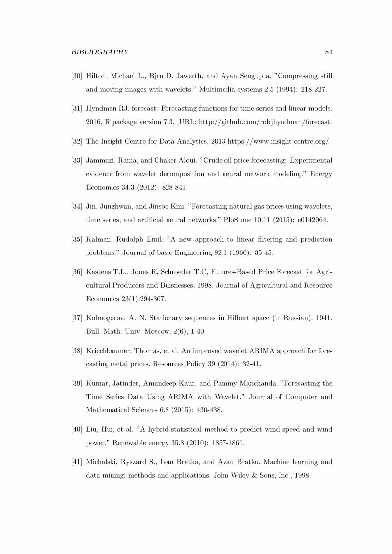
BIBLIOGRAPHY 84

[30] Hilton, Michael L., Bjrn D. Jawerth, and Ayan Sengupta. ”Compressing still

and moving images with wavelets.” Multimedia systems 2.5 (1994): 218-227.

[31] Hyndman RJ. forecast: Forecasting functions for time series and linear models.

2016. R package version 7.3, ¡URL: http://github.com/robjhyndman/forecast.

[32] The Insight Centre for Data Analytics, 2013 https://www.insight-centre.org/.

[33] Jammazi, Rania, and Chaker Aloui. ”Crude oil price forecasting: Experimental

evidence from wavelet decomposition and neural network modeling.” Energy

Economics 34.3 (2012): 828-841.

[34] Jin, Junghwan, and Jinsoo Kim. ”Forecasting natural gas prices using wavelets,

time series, and artificial neural networks.” PloS one 10.11 (2015): e0142064.

[35] Kalman, Rudolph Emil. ”A new approach to linear filtering and prediction

problems.” Journal of basic Engineering 82.1 (1960): 35-45.

[36] Kastens T.L., Jones R, Schroeder T.C, Futures-Based Price Forecast for Agri-

cultural Producers and Buisnesses, 1998, Journal of Agricultural and Resource

Economics 23(1):294-307.

[37] Kolmogorov, A. N. Stationary sequences in Hilbert space (in Russian). 1941.

Bull. Math. Univ. Moscow, 2(6), 1-40

[38] Kriechbaumer, Thomas, et al. An improved wavelet ARIMA approach for fore-

casting metal prices. Resources Policy 39 (2014): 32-41.

[39] Kumar, Jatinder, Amandeep Kaur, and Pammy Manchanda. ”Forecasting the

Time Series Data Using ARIMA with Wavelet.” Journal of Computer and

Mathematical Sciences 6.8 (2015): 430-438.

[40] Liu, Hui, et al. ”A hybrid statistical method to predict wind speed and wind

power.” Renewable energy 35.8 (2010): 1857-1861.

[41] Michalski, Ryszard S., Ivan Bratko, and Avan Bratko. Machine learning and

data mining; methods and applications. John Wiley & Sons, Inc., 1998.

BIBLIOGRAPHY 85

[42] McCarren A., McCarthy S., O. Sullivan C., and Roantree M. Anomaly detection

in agri warehouse construction. Procedings of ACSW 2017, ACM Press 17,

doi¿10.1145/3014812.3014829.

[43] Nau, Robert, Statistical forecasting: Notes on regression and time series anal-

ysis, https://people.duke.edu/ rnau/411arim.htm

[44] Nguyen, Hang T., and Ian T. Nabney. Short-term electricity demand and gas

price forecasts using wavelet transforms and adaptive models. Energy 35.9

(2010): 3674-3685.

[45] OMIE Download page for Spanish Electricity Historical Prices

http://www.omie.es/files/flash/ResultadosMercado.swf

[46] Pankratz, Alan. Forecasting with univariate Box-Jenkins models: Concepts and

cases. Vol. 224. John Wiley & Sons, 2009.

[47] Parzen, E. ARARMA models for time series analysis and forecasting. Journal

of Forecasting, 1982 vol. 1, 67-82.

[48] Percival, D. and Walden, A. (2000) Wavelet Methods for Time Series Analysis.

Cambridge, UK: Cambridge University Press.

[49] Pizurica, Aleksandra, et al. ”A versatile wavelet domain noise filtration tech-

nique for medical imaging.” IEEE transactions on medical imaging 22.3 (2003):

323-331.

[50] R Core Team, R: A Language and Environment for Statistical Computing,

2016, https://www.R-project.org/.

[51] Ramsey, James B. ”The contribution of wavelets to the analysis of economic and

financial data.” Philosophical Transactions of the Royal Society of London A:

Mathematical, Physical and Engineering Sciences 357.1760 (1999): 2593-2606.

[52] Schleicher, Christoph. An introduction to wavelets for economists. Bank of

Canada, 2002.

BIBLIOGRAPHY 86

[53] Seo, In-Yong, et al. ”Short Term Wind Power Prediction Using Wavelet Trans-

form and ARIMA.” Journal of Energy and Power Engineering 6.11 (2012):

1786.

[54] Shafie-Khah, M., M. Parsa Moghaddam, and M. K. Sheikh-El-Eslami. ”Price

forecasting of day-ahead electricity markets using a hybrid forecast method.”

Energy Conversion and Management 52.5 (2011): 2165-2169.

[55] Stevenson, Simon. ”A comparison of the forecasting ability of ARIMA models.”

Journal of Property Investment & Finance 25.3 (2007): 223-240.

[56] https://www.teagasc.ie, 2016.

[57] Wei, Dong. Coiflet-type wavelets: theory, design, and applications. Diss. Uni-

versity of Texas at Austin, 1998.

[58] Wiener, N. Non-linear problems in random theory. (1958). Wiley.

[59] Yousefi, Shahriar, Ilona Weinreich, and Dominik Reinarz. Wavelet-based pre-

diction of oil prices. Chaos, Solitons & Fractals 25.2 (2005): 265-275.

[60] Yule, G. U. On the method of investigating periodicities in disturbed series,

with special reference to Wolfers sunspot numbers. Philosophical Transactions

of the Royal Society London, 1927, Series A, 226, 267-298

[61] Zhongfu T., et al. Day-ahead electricity price forecasting using wavelet trans-

form combined with ARIMA and GARCH models. Applied Energy 87.11

(2010): 3606-3610.

[62] Zhu, Li, Yanxin Wang, and Qibin Fan. MODWT-ARMA model for time series

prediction. Applied Mathematical Modelling 38.5 (2014): 1859-1865.

A Combined Wavelet and ARIMA Approach to Predicting Financial Time...

Documents

Transcript of A Combined Wavelet and ARIMA Approach to Predicting Financial Time...