7.1 Basic Properties of Confidence Intervals

What’s Missing in a Point Estimate?

• Just a single estimate

• No idea how reliable this estimate is

• What we need:

• how reliable it is

• some measure of the variability

Ideas behind CI

• Realizing that a single estimate is insufficient

• Try to use an interval to cover our target

• Crucial aspects:

• how reliable is this interval? - confidence level

• how meaningful is this interval? - width

Introducing Confidence Intervals for population mean

• Start with the sample mean

• We have

• If X is normal,

X̄ =X1 + X2 + · · · + Xn

n

E[X̄] = µ, V [X̄] =σ2

n

P

�����X̄ − µ

σ/√

n

���� < zα/2

�= 1− α

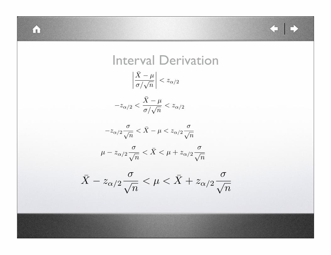
Interval Derivation����X̄ − µ

σ/√

n

���� < zα/2

−zα/2 <X̄ − µ

σ/√

n< zα/2

−zα/2σ√n

< X̄ − µ < zα/2σ√n

µ− zα/2σ√n

< X̄ < µ + zα/2σ√n

X̄ − zα/2σ√n

< µ < X̄ + zα/2σ√n

Interpreting CI

• Notice only is random, not

• Interval is random

• The probability that this random interval covers is

• If we repeat the experiment many many times, we should have of the intervals covering

• Typical values: 90%, 95%, 99%...

X̄ µ

µ

1− α

1− α

100(1− α)%

µ

Common Misconceptions

• Say 95%, , one interval (1.5,1.8)obtained from a sample

• False claims:

• there is a 95% chance that is in this interval

• 95% of the observations are in this interval

• both are wrong!

z0.025 = 1.96

µ

Calculating the Bounds

• Determine the needed

• Check the normal distribution requirement

• See if is available (most likely not, so approximation is needed)

α

σ

�x̄− zα/2

σ√n

, x̄ + zα/2σ√n

�

x̄± zα/2σ√n

Examples

• (a). 95%: ,

• (b). 99%:

• more confidence, wider interval, less useful!

x̄ = 58.3, n = 50,σ = 3

z0.025 = 1.96 z0.025σ√n

= 1.96× 3√50

= 0.832

(57.47, 59.13)z0.005 = 2.57, z0.005

σ√n

= 2.57× 3√50

= 1.09

(57.2, 59.39)

Role of Sample Size n• Everything else being equal

• n increased by 4 times - interval narrowed by half

• n decreased by 4 times - interval enlarged by double

• if a particular w (width) is required

n =�2zα/2 · σ

w

�2

7.2 Large-Sample CI for a Population Mean and

Proportion

Conditions for Previous CI Discussion

• Focused on population mean

• Assume the population distribution to be normal

• Require random samples

• Population variance is assumed to be known

• Approximation of by is often used, assuming large sample size

µ

(X1, X2, . . . , Xn)

σ2

σ2 S2

n

Getting around the normal

• No reason to assume a normal distribution in practice (example, the proportion of successes)

• Often the estimator can be approximately normal if the sample size is large enough (CLT at work!)

• Formulas are similar, but the implications can be subtle

Large-Sample Interval for

• Estimator

• Approximately normal if n is large

• Standardize

• Large-Sample CI for

µ

X̄

Z =X̄ − µ

σ/√n

P�−zα/2 < Z < zα/2

�= 1− α

µ

x̄± zα/2 ·s√n

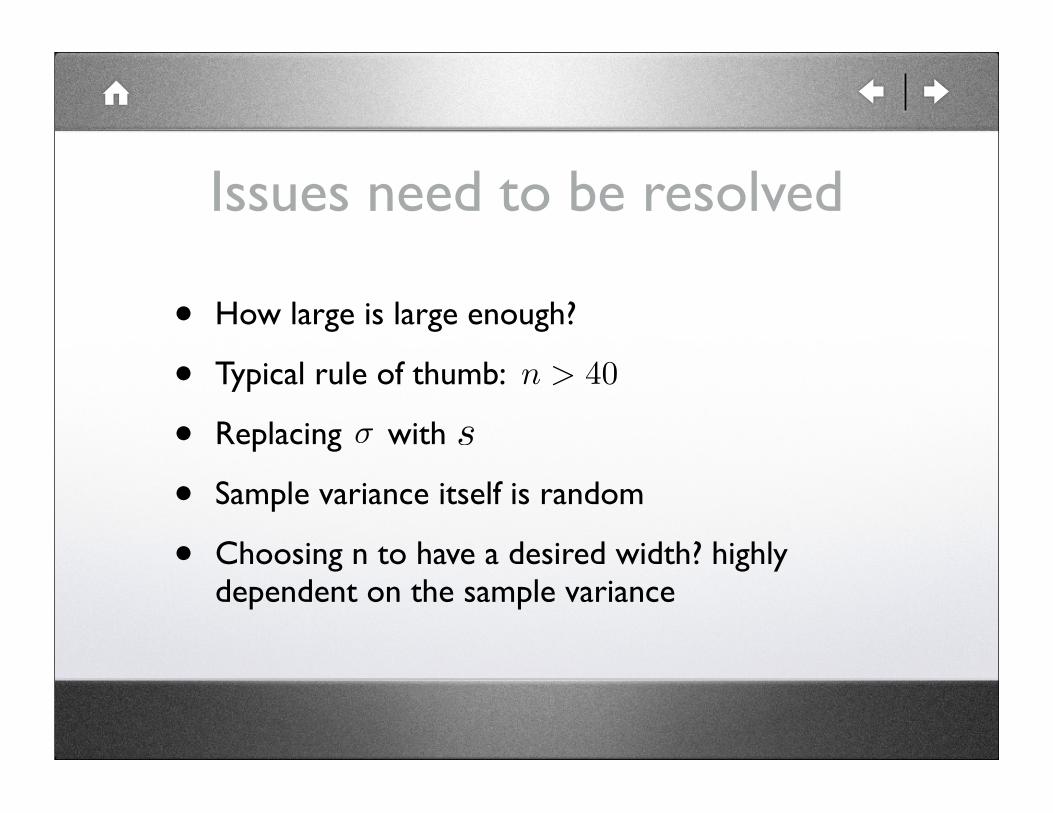
Issues need to be resolved

• How large is large enough?

• Typical rule of thumb:

• Replacing with

• Sample variance itself is random

• Choosing n to have a desired width? highly dependent on the sample variance

n > 40

σ s

From to more general parameters

• Consider more general

• Do we still have an estimator that is approximately normal?

• Require

• approximately normal

• unbiased

• an expression for

µ

θ

σθ̂

θ̂

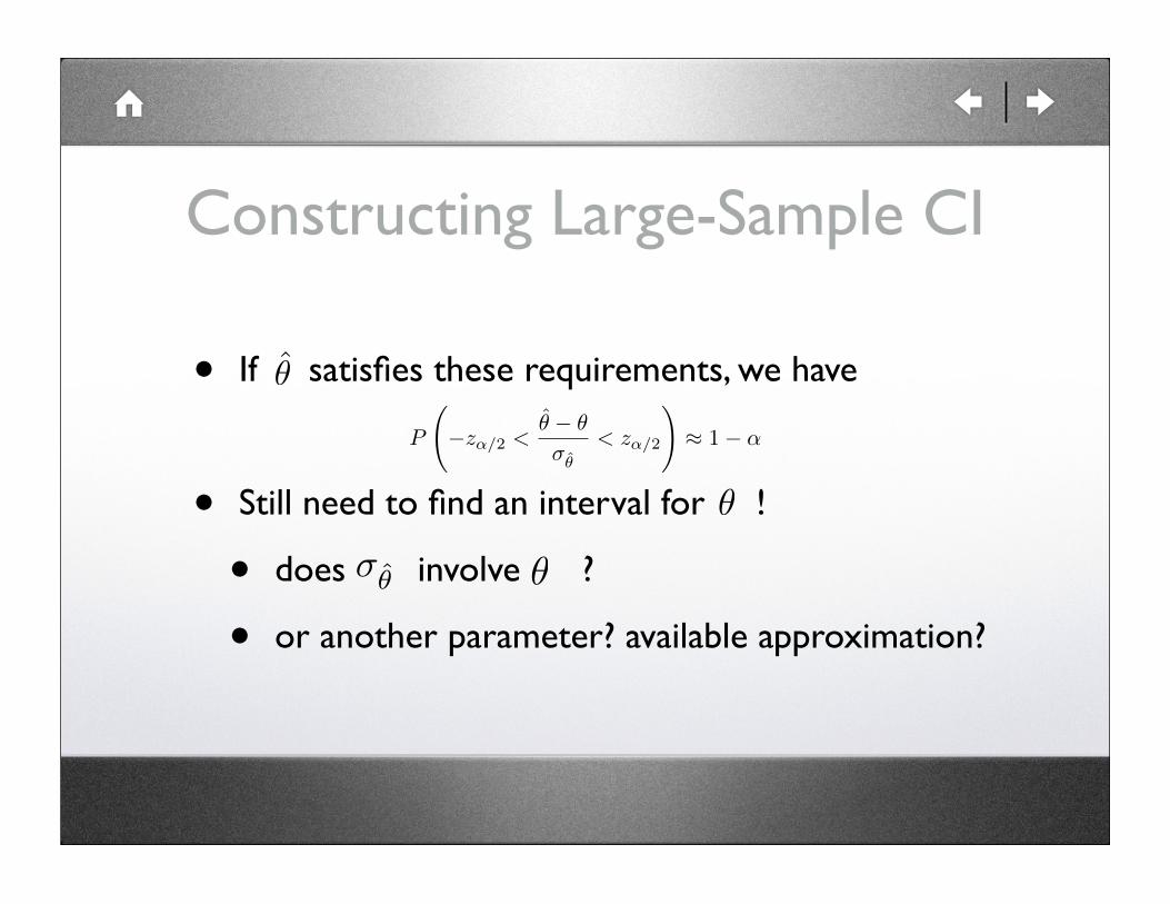
Constructing Large-Sample CI

• If satisfies these requirements, we have

• Still need to find an interval for !

• does involve ?

• or another parameter? available approximation?

P

�−zα/2 <

θ̂ − θ

σθ̂

< zα/2

�≈ 1− α

θ

σθ̂ θ

θ̂

CI for Population Proportion

• Parameter in question: population proportion

• Natural estimator:

• Expression for

• Solve for the CI:

θ = p

p̂ = X/n

σθ̂

σp̂ =�p(1− p)/n

p =p̂+

z2α/2

2n ± zα/2

�p̂q̂n +

z2α/2

4n2

1 + (z2α/2)/n

Two Different CI’s for p

• More accurate

• More simplified

• Advantages of the first: (1) closer to the the intended confidence level; (2) even works with sample sizes not so large!

p =p̂+

z2α/2

2n ± zα/2

�p̂q̂n +

z2α/2

4n2

1 + (z2α/2)/n

p = p̂± zα/2�p̂q̂/n

One-Sided CI (Confidence Bounds)

• large-sample upper CB

• large-sample lower CB

•

µ < x̄+ zαs√n

µ > x̄− zαs√n

7.3 Intervals Based on Normal Population

Distribution

Key Assumptions

• Normal population distribution

• Population standard dev NOT known, so sample standard dev is used

• Sample size not large!

• Problem: is NOT normal!

σS

X̄ − µ

S/√

n

A New Distribution

• What do we know about this distribution?

• more variability than the normal - more spread

• additional parameter: the number of degree of freedom (df) = n-1, where n is the sample size

• Student’s t-distribution, or just the t-distribution

Properties of t Distribution

• Denote the density function curve for df

• Each curve is bell-shaped, centered at 0

• Each curve is more spread out than the standard normal curve

• As increases, the spread decreases

• As , the sequence of curves approaches the standard normal curve

ν

ν

ν →∞

tν

tν

tν

tν

Standardize the rv

• We use the following in place of Z

• T has the t distribution with df n-1 where n is the sample size

• As n becomes large, T can be replaced by Z

T =X̄ − µ

S/√

n

Probability Statement

• Replacing with

• is the location on measurement axis for which the area under the curve to the right of is

• is called a t critical value

• Different df leads to different critical values

zα tα,ν

tα,ν

tα,ν

tα,ν α

One-Sample t CI

• confidence interval for is

• Upper confidence bound

• lower confidence bound

• Can we find the n to give a desired interval width?

100(1− α) µ�

x̄− tα/2,n−1 · s√n

, x̄ + tα/2,n−1 · s√n

�

x̄ + tα,n−1 · s√n

x̄− tα,n−1 · s√n

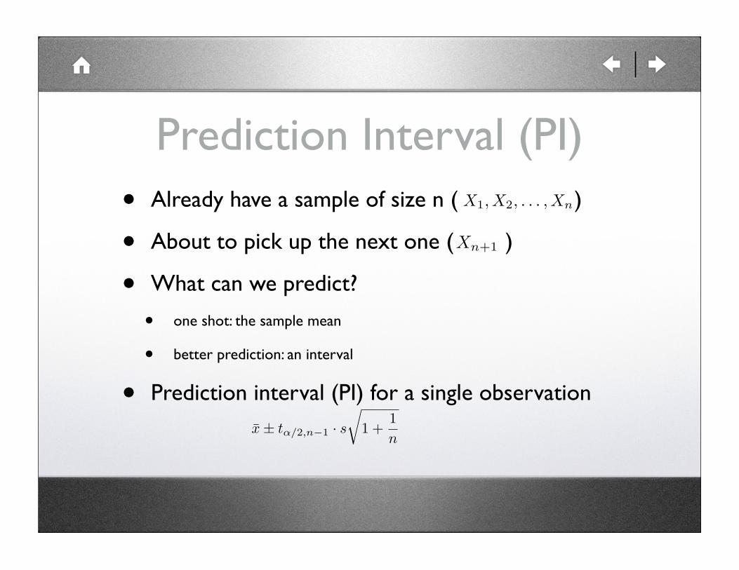
Prediction Interval (PI)• Already have a sample of size n ( )

• About to pick up the next one ( )

• What can we predict?

• one shot: the sample mean

• better prediction: an interval

• Prediction interval (PI) for a single observation

X1, X2, . . . , Xn

Xn+1

x̄ ± tα/2,n−1 · s�

1 +1n

Tolerance Intervals

• Want to find an interval that captures certain percentage of the values in a normal distribution

• Allow some uncertain factor (confidence level)

• Tolerance interval for capturing at least k% of the values, with a confidence level 95%

• Critical values found in Appendix Table A.6

x̄ ± (tolerance critical value) · s

7.4 CIs for Variance and Standard Dev of a Normal

Population

Estimating Variance

• always needed in estimation of other parameters

• A point estimate often suffices, but sometimes we would like to have a CI

• Distribution of S usually more complicated than that of X̄

σ

Normal Population Assumption

• We need to start from something familiar

• Population with normal distribution

• is normal, but is not

• chi-square distribution

• Another parameter involved (df)

X̄ S

χ2

A Theorem

• Let be a random sample from a normal distribution

• the rv

• has a chi-square distribution with n-1 df

X1, X2, . . . , Xn

N(µ,σ2)

(n− 1)S2

σ2=

�(Xi − X̄)2

σ2

chi-squared critical values

• similar ideas as

• additional parameter - df (n-1 in our applications)

• denotes the number of the measurement axis such that of the area under the curve with df lies to the right of

zα, tα,ν

χ2α,ν

χ2α,ν

α ν

What’s different?

• not symmetric, because it is positive, but unbounded in the positive direction

• Two ends:

• lower - , upper -

• Interval for , confidence level

• Formulas for one-sided:

(n− 1)S2

χ2α/2,n−1

< σ2 <(n− 1)S2

χ21−α/2,n−1

χ21−α/2,n−1 χ2

α/2,n−1

χ2

σ2 100(1− α)%

α/2→ α