6.207/14.15: 4, 5 6: Linear Dynamics, Markov Chains ...
44
6.207/14.15: Networks Lectures 4, 5 & 6: Linear Dynamics, Markov Chains, Centralities 1
Transcript of 6.207/14.15: 4, 5 6: Linear Dynamics, Markov Chains ...

6.207/14.15: Networks Lectures 4, 5 & 6: Linear Dynamics, Markov Chains,
Centralities
1

��
���
���
��
Networks: Lectures 4, 5 & 6 Outline
Outline
Dynamical systems. Linear and Non-linear. Convergence. Linear algebra and Lyapunov functions.
Markov chains. Positive linear systems. Perron-Frobenius. Random walk on graph.
Centralities. Eigen centrality. Katz centrality. Page Rank. Hubs and Authorities.
Reading: Newman, Chapter 6 (Sections 6.13-14). Newman, Chapter 7 (Sections 7.1-7.5).
2
���
� �
�
���
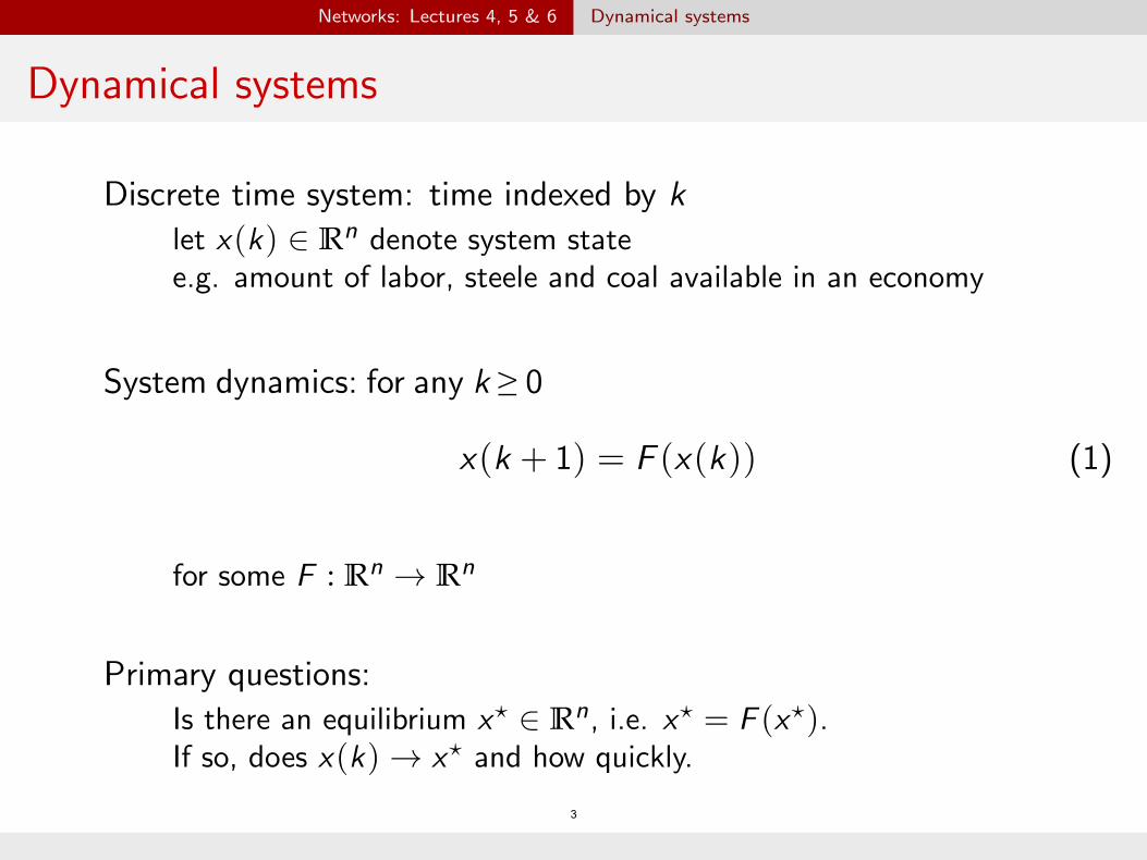
Networks: Lectures 4, 5 & 6 Dynamical systems
Dynamical systems
Discrete time system: time indexed by k let x(k) 2 Rn denote system statee.g. amount of labor, steele and coal available in an economy
System dynamics: for any k ≥ 0
x(k + 1) = F (x(k)) (1)
for some F : Rn ! Rn
Primary questions: ?Is there an equilibrium x? 2 Rn, i.e. x = F (x?).
If so, does x(k) ! x? and how quickly. 3

� �
��
���
��
Networks: Lectures 4, 5 & 6 Dynamical systems
Linear dynamical systems
Linear system dynamics: for any k ≥ 0
x(k + 1) = Ax(k) + b (2)
for some A 2 Rn⇥n and b 2 Rn
example: Leontif’s input-output model of economy
We’ll study Existence and characterization of equilibrium. Convergence.
Initially, we’ll consider b = 0 Later, we shall consider generic b 2 Rn
4

��
�
�
�
Networks: Lectures 4, 5 & 6 Dynamical systems
Linear dynamical systems
Consider
x(k) = Ax(k – 1) = A ⇥ Ax(k – 2)· · ·= Ak x(0)
So what is Ak ?
For n = 1, let A = a 2 R+:80 if 0 a < 1>
k
k!•<
x(k) = a x(0) ! x(0) if a = 1>• if 1 < a.:
5
�
�
��
Networks: Lectures 4, 5 & 6 Dynamical systems
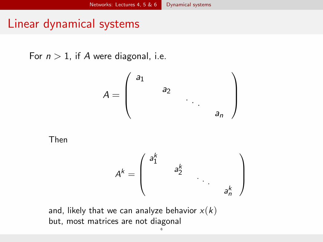
Linear dynamical systems
For n > 1, if A were diagonal, i.e. 0
BB
1
CCa1
a2A = @ . . .an
A
Then 0
BB
1
CC
ka1ak2Ak = @ . . .
a
Ak
n
and, likely that we can analyze behavior x(k) but, most matrices are not diagonal
6
�� �
�
��
�
�
Networks: Lectures 4, 5 & 6 Dynamical systems
Linear dynamical systems
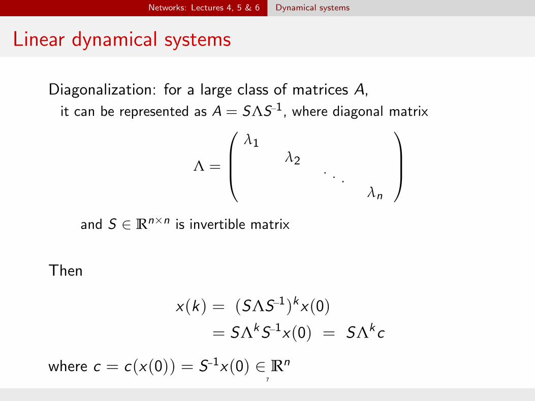
Diagonalization: for a large class of matrices A,
0
BBl1
l2
1it can be represented as A = SLS–1, where diagonal
matrix
CCL = @ . . .ln
A
and S 2 Rn⇥n is invertible matrix
Then
x(k) = (SLS–1)k x(0) = SLk S–1 x(0) = S Lk c
where c = c(x(0)) = S–1x(0) 2 Rn
7

�
�
Networks: Lectures 4, 5 & 6 Dynamical systems
Linear dynamical systems
Suppose
S =
0
@s1 . . . sn
1
A
Then
x(k) = SLk c n
= Â ci lk
i sii=1
8

� �
� �
�
�
� �
Networks: Lectures 4, 5 & 6 Dynamical systems
Linear dynamical systems
Let 0 |ln
| |ln 1| · · · |l2| < |l1|
Then 80 if |l1| < 1>
k!•<
kx(k)k ! |c1|ks1k if |l1| = 1>:• if |l1| > 1
moreover, for |l1| > 1,
k
kl 1 x(k) – c1s1k ! 0.9
x(k) =n
Âi=1
ci
li
ksi
= lk
1
⇣c1s1 +
n
Âi=2
ci
� li
l1
�k
si
⌘

���
�� ��
���
��
Networks: Lectures 4, 5 & 6 Dynamical systems
Diagonalization
When can a matrix A 2 Rn⇥n be diagonalize?When A has n distinct eigenvalues, for example In general, all matrices are block-diagonalizable a la Jordan form
Eigenvalues of A Roots of n order (characteristic) polynomial: det(A – lI ) = 0 Let they be l1, . . . , l
n
Eigenvectors of A Given l
i , let si 6= 0 be such that As
i = li si
Then si is eigenvector corresponding to eigenvalue l
i
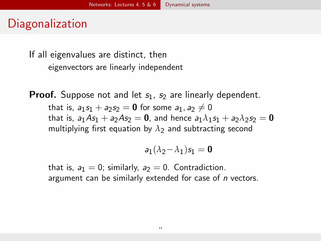
If all eigenvalues are distinct, then eigenvectors are linearly independent
10
��
����
�
��
Networks: Lectures 4, 5 & 6 Dynamical systems
Diagonalization
If all eigenvalues are distinct, then eigenvectors are linearly independent
Proof. Suppose not and let s1, s2 are linearly dependent. that is, a1s1 + a2s2 = 0 for some a1, a2 6= 0that is, a1As1 + a2As2 = 0, and hence a1l1s1 + a2l2s2 = 0 multiplying first equation by l2 and subtracting second
a1(l2 – l1)s1 = 0
that is, a1 = 0; similarly, a2 = 0. Contradiction. argument can be similarly extended for case of n vectors.
11

��
�
�
Networks: Lectures 4, 5 & 6 Dynamical systems
Diagonalization
If all eigenvalues are distinct (li 6= l
j , i 6= j), theneigenvectors, s1, . . . , s
n
, are linearly independent
Therefore, we have invertible matrix S , where
S =
0
@s1 . . . sn
1
A
Consider diagonal matrix of eigenvalues 0
@ l1
1
AL = . . .ln
12
�
� �
�
Networks: Lectures 4, 5 & 6 Dynamical systems
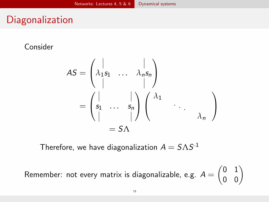
Diagonalization
Consider
AS
0
@
0
@
1
Al1s1 . . . ln
sn =
s1 . . . sn
0
@
1
A
1
A l1
.= . .ln
✓0 1
= SL
Therefore, we have diagonalization A = SLS–1
Remember: not every matrix is diagonalizable, e.g. A = 0 0
◆
13

�
� �
�� �
� � � �
�
Networks: Lectures 4, 5 & 6 Dynamical systems
Linear dynamical systems
Let us consider linear system with b 6= 0:
x(k + 1) = Ax(k) + b
= A(Ax(k – 1) + b) + b = A2 x(k – 1) + (A + I )b . . .
⇣ k – 1
 –1⌘b.= Ak Ak – jx(0) +
k – 1n
Â
j=0
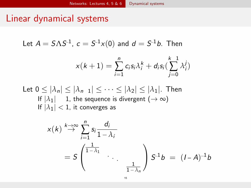
Let A = SLS–1, c = S–1x(0) and d = S–1b. Then
 jci si l
k
i
x(k + 1) = + di si ( l )
i i =1 j=0
14
� � � �
�
� �� ��
�
�
�
� � �
Networks: Lectures 4, 5 & 6 Dynamical systems
Linear dynamical systems
Let A = SLS–1, c = S–1x(0) and d = S–1b. Then
=0 Â
k 1n
 j
jci si l
k
i
x(k + 1) = + di si ( )l
i i =1
Let 0 |ln
| |ln 1| · · · |l2| |l1|. Then
If |l1| 1, the sequence is divergent (! •) If |l1| < 1, it converges as
n diÂk!•
x(k) ! si
1 – li
i=1 0
@ 1
1 – l1
1
A= S . . .1
1 – ln
S–1b = (I – A)–1b
15

�
�
� �
�
Networks: Lectures 4, 5 & 6 Dynamical systems
Linear dynamical systems
For linear system, equilibrium x? should satisfy
x ? = Ax? + b
The solution to the above exists when A does not have an eigenvalue equal to 1, which is
x ? = (I – A)–1b
But, as discussed, it may not be reached unless |l1| < 1!
16

�
�
�
�
�
Networks: Lectures 4, 5 & 6 Dynamical systems
Nonlinear dynamical systems
Consider nonlinear system
x(k + 1) = F (x(k)) = x(k) + (F (x(k)) – x(k)) = x(k) + G (x(k))
where G (x) = F (x) – x
Continuous approximation of the above (replace k by time index t)
dx(t) = G (x(t))
dt
When does x(t) ! x??17

�
�
�
Networks: Lectures 4, 5 & 6 Dynamical systems
Lyapunov function
Let there exist a Lyapunov (or Energy) function V : Rn ! R+
Such that
?1. V is minimum at x
dV (x(t)) ?2. dt < 0 if x(t) 6= x
?that is, rV (x(t))T
G (x(t)) < 0 if x(t) 6= x
?Then x(t) ! x
18

���
�
�
�
�
Networks: Lectures 4, 5 & 6 Dynamical systems
Lyapunov function: An Example
A simple model of Epidemic Let I (k) 2 [0, 1] be fraction of population that is infectedand S(k) 2 [0, 1] be the fraction of population that is susceptible toinfection Population is either infected or susceptible: I (k) + S(k) = 1
Due to “social interaction” they evolve as
I (k + 1) = I (k) + bI (k)S(k) S(k + 1) = S (k) – bI (k)S(k)
where b 2 (0, 1) is a parameter captures “infectiousness”
Question: what is the equilibrium of such a society? 19

�
�
� �
�
� �
�
Networks: Lectures 4, 5 & 6 Dynamical systems
Lyapunov function: An Example
Since I (k) + S(k) = 1, we can focus only on one of them, say S(k)
Then
S(k + 1) = S (k) – b(1 – S(k))S(k)
That is, continuous approximation suggests
dS(t) = – b(1 – S(t))S(t).
dt
An easy Lyapunov function is V (S) = S
20

�
� �
�
�
�
Networks: Lectures 4, 5 & 6 Dynamical systems
Lyapunov function: An Example
For V (S) = S :
dV (S(t)) dS(t)= V 0(S(t))
dt dt = b(1 – S(t))S(t)
Then, for S(t) 2 [0, 1) if S(t) 6= 0,
dV (S(t)) < 0
dt
And V is minimized at 0
Therefore, if S(0) < 1, then S(t) ! 0: entire population is infected!21

���
� �
��
�
���
Networks: Lectures 4, 5 & 6 Positive linear system
Positive linear system
Positive linear system Let A = [A
ij ] 2 Rn⇥n be such that Aij > 0 for all 1 i , j n
System dynamics:
x(k) = Ax(k – 1), for k ≥ 1.
Perron-Frobenius Theorem: let A 2 Rn⇥n be positiveLet l1, . . . , l
n be eigenvalues such that
0 |ln
| |ln 1| · · · |l2| |l1|
Then, maximum eigenvalue l1 > 0 It is unique, i.e. |l1| > |l2|Corresponding eigenvector, say s1 is component-wise > 0
22

�� ��
� ��
��� �
�� ��
���
�
Networks: Lectures 4, 5 & 6 Positive linear system
Perron Frobenius Theorem
23
� Why is l1 > 0?
�TLet
isTnon= {t-emp
>ty:0 :AAx �
=txmi,nfor
Asome
Txbe2cRa
n
u+s}e� min ij ij
2� A1 � Amin1 and Amin > 0 since A > 0
� T is bounded because
�?Ax 6� nAmaxx for any x 2 Rn
+, where Amax = max
ij
A
ij
� LetThat
tis,=tmaxhere
{tex
:istts2x
T}� 2 Rn
+?
such that Ax � t?x� In fact, it must be Ax = t x .
� Because, if Ax � t
?x
?, then A
2x > t
?Ax beca
T
use A > 0
� This will contradict t being maximum over
� For any eigenvalue, eigenvector pair (l, z), i.e. Az = lz� |
th
le
||re
z |fo
=re,
|Azl|
t
A
?|z |
� | | � Thus, we have established that eigenvalue with largest norm is t? > 0.
����
����
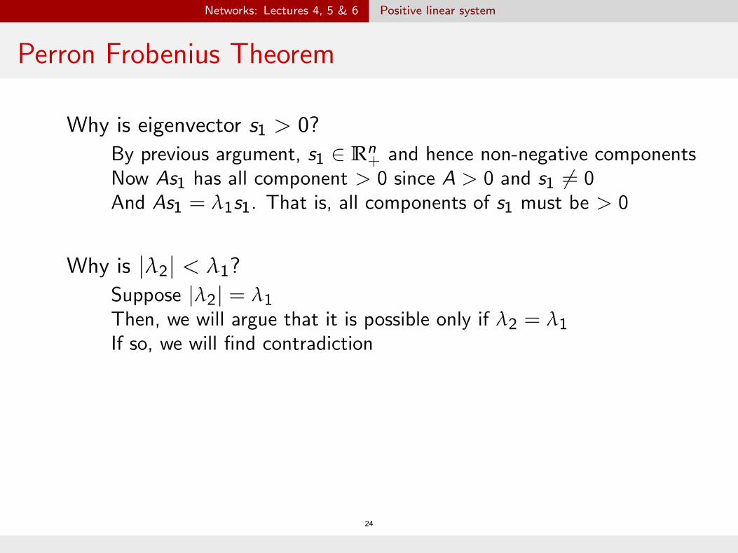
Networks: Lectures 4, 5 & 6 Positive linear system
Perron Frobenius Theorem
Why is eigenvector s1 > 0? By previous argument, s1 2 Rn and hence non-negative components+ Now As1 has all component > 0 since A > 0 and s1 6= 0 And As1 = l1s1. That is, all components of s1 must be > 0
Why is |l2| < l1?
Suppose |l2| = l1
Then, we will argue that it is possible only if l2 = l1
If so, we will find contradiction
24
��� �� ��� �
� �� ��
��
���
� �
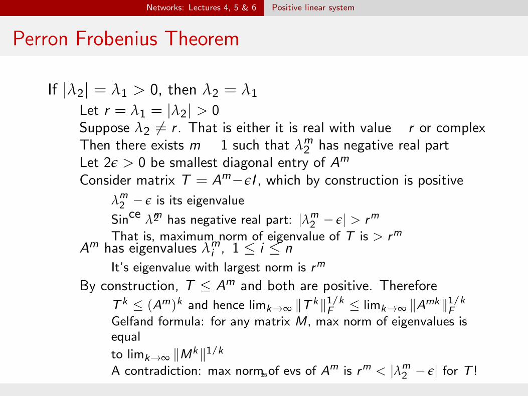
Networks: Lectures 4, 5 & 6 Positive linear system
Perron Frobenius Theorem
If |l2| = l1 > 0, then l2 = l1
Let r = l1 = |l2| > 0 Suppose l2 6= r . That is either it is real with value r or complexThen there exists m 1 such that lm has negative real part 2 Let 2e > 0 be smallest diagonal entry of Am
Consider matrix T = Am – eI , which by construction is positive l2m
– e is its eigenvaluece 2
Sin lm has negative real part: |l2
m
– e| > rmThat is, maximum norm of eigenvalue of T is > rm
Am has eigenvalues lm, 1 i ni
m
It’s eigenvalue with largest norm is rBy construction, T Am and both are positive. Therefore
T k (Am)k and hence lim
k!• kT k k1/k limk!• kAmk k1/k
F F Gelfand formula: for any matrix M, max norm of eigenvalues i s equal
to limk!• kMk k1/k
A contradiction: max norm of evs of Am is rm < |l2
m
– e| for T !25
���� �� �� ��
��
�
Networks: Lectures 4, 5 & 6 Positive linear system
Perron Frobenius Theorem
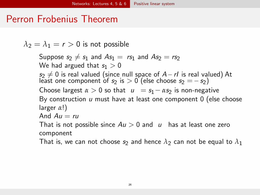
l2 = l1 = r > 0 is not possible Suppose s2 6= s1 and As1 =
rs1 and As2 = rs2
We had argued that s1 > 0s2 6= 0 is real valued (since null space of A – rI is real value
d) At
least one component of s2 is > 0 (else choose s2 = – s 2)
Choose largest a > 0 so that u = s1 – as2 is non-negativeBy construction u must have at least one component 0 (else choose larger a!) And Au = ru That is not possible since Au > 0 and u has at least one zero component That is, we can not choose s2 and hence l2 can not be equal to l1
26
�� �� ����
���
Networks: Lectures 4, 5 & 6 Positive linear system
Positive linear system
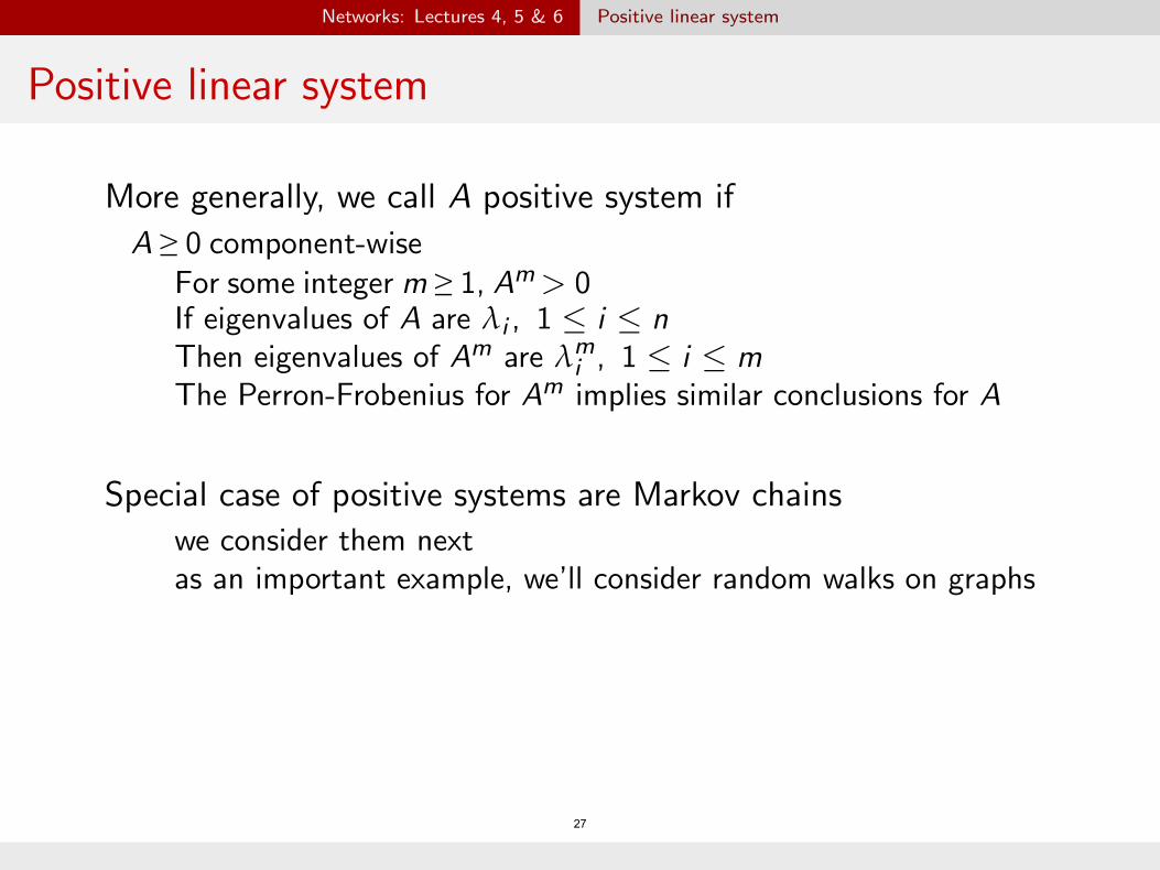
More generally, we call A positive system if A ≥ 0 component-wise
For some integer m ≥ 1, Am > 0 If eigenvalues of A are l
i , 1 i nThen eigenvalues of Am are lm, 1 i m
i The Perron-Frobenius for Am implies similar conclusions for A
Special case of positive systems are Markov chains we consider them next as an important example, we’ll consider random walks on graphs
27

�
��
��
Networks: Lectures 4, 5 & 6 Markov chains
An Example
Shu✏ing cards
A special case of Overhead shu✏e: choose a card at random from deck and place it on top
How long does it take for card deck to become random? Any one of 52! orderings of cards is equally likely
28
�
�� �
Networks: Lectures 4, 5 & 6 Markov chains
An Example
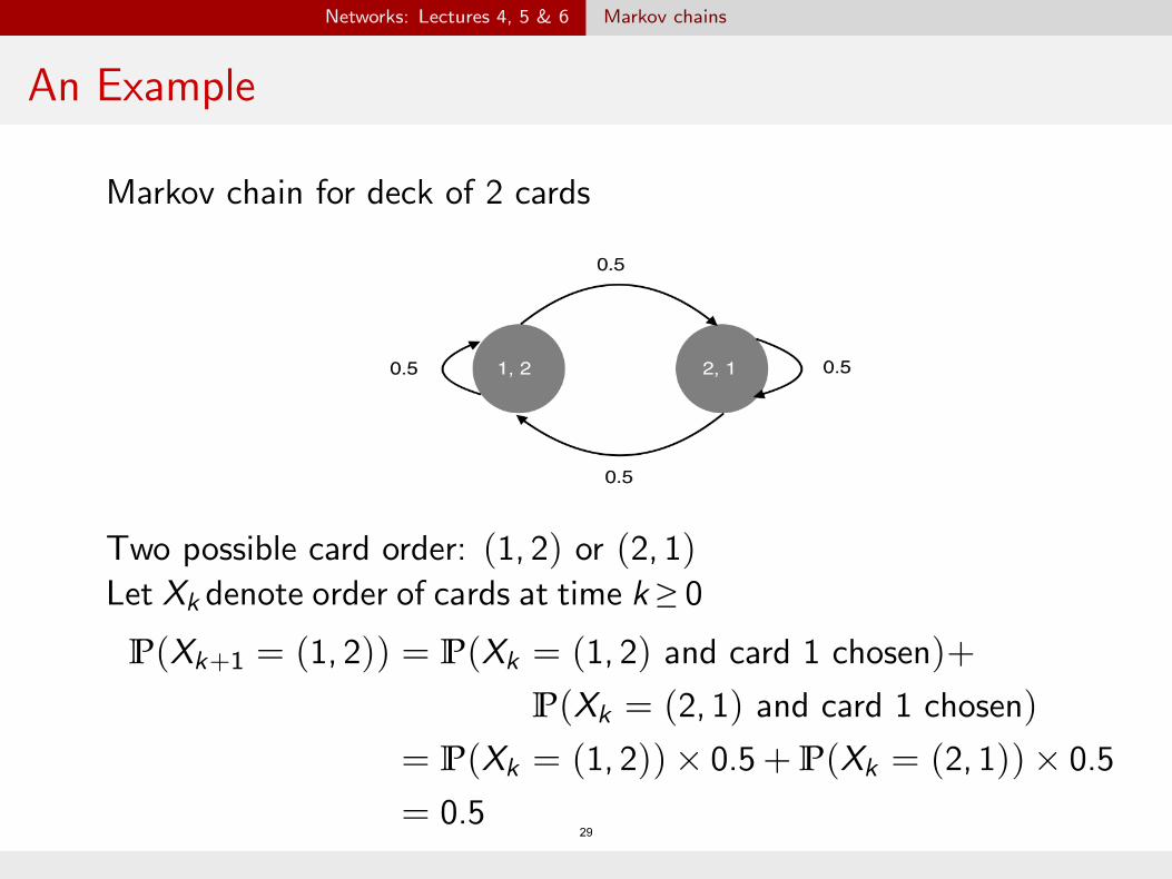
Markov chain for deck of 2 cards
Two possible card order: (1, 2) or (2, 1) Let X
k denote order of cards at time k ≥ 0
P(Xk+1 = (1, 2)) = P(X
k = (1, 2) and card 1 chosen)+ P(X
k = (2, 1) and card 1 chosen) = P(X
k = (1, 2)) ⇥ 0.5 + P(Xk = (2, 1)) ⇥ 0.5
= 0.5 29

�� �� �
�
�� ��
Networks: Lectures 4, 5 & 6 Markov chains
Notations
Markov chain defined over state space N = {1, . . . , n} X
k 2 N denote random variable representing state at ti me k ≥ 0
Pij = P(X
k+1 = j |Xk = i) for all i , j 2 N and all k ≥ 0
P(Xk+1 = i) = Â Pji P(X
k = j)j2N
Let p(k) = [pi (k)] 2 [0, 1]n, where p
i (k) = P(Xk = i)
pi (k + 1) = Â pj (k)Pji , 8i 2 N , p(k + 1)T = p(k)T P
j2N
P = [Pij ]: probability transition matrix of Markov chain
non-negative: P ≥ 0 row-stochastic: Â
j2N Pij = 1 for all i 2 N
30

����
���
� �
�
Networks: Lectures 4, 5 & 6 Markov chains
Stationary distribution
Markov chain dynamics: p(k + 1) = PT p(k) Let P > 0 (PT > 0): positive linear system Perron-Frobenius: PT has unique largest eigenvalue: lmax > 0
? ?Let p? > 0 be corresponding eigenvector: PT p = lmaxp?We claim lmax = 1 and p(k) ! p
Recall, kp(k)k ! 0 if lmax < 1 or kp(k)k ! • if lmax > 1But Â
i pi (k) = 1 for all k , since Âi pi (0) = 1 and
 pi (k + 1) = p(k + 1)T 1 = p(k)T P1
i
= Â pi (k)Pij = Â pi (k) Â Pij
ij i j
= Â pi (k).i
Therefore, lmax must be 1 and p(k) ! p? (as argued before)31
�
� �� ��
��
�
�
Networks: Lectures 4, 5 & 6 Markov chains
Stationary distribution
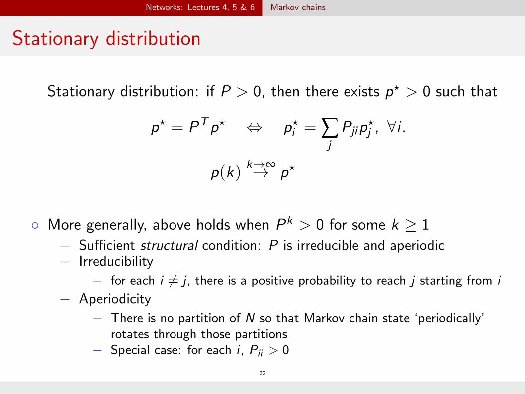
Stationary distribution: if P > 0, then there exists p? > 0 such that
? ? ? ? p = PT p , p = Â Pji pj , 8i .i
j
k!• ?p(k) ! p
32
� More generally, above holds when Pk > 0 for some k � 1
� Su�cient structural condition: P is irreducible and aperiodic� Irreducibility
� for each i 6= j , there is a positive probability to reach j starting from i
� Aperiodicity
� There is no partition of N so that Markov chain state ‘periodically’
rotates through those partitions
� Special case: for each i , P
ii
> 0

� ��
�
�
Networks: Lectures 4, 5 & 6 Markov chains
Stationary distribution
There exists q = [qi ] > 0 such
Reversible Markov chain with transition matrix P ≥ 0
qi Pij = q
j Pji , 8 i 6= j 2 N (3)
Then, stationary distribution, p? exists such that
Because, by (3) and P being stochastic
 qj Pji =  qi Pij
j j
= qi (Â Pij )
j
= qi
33
p? =1
(Âi
qi
)q
���
���
�
Networks: Lectures 4, 5 & 6 Graph dynamics, centrality
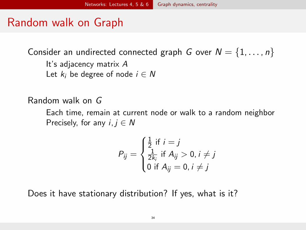
Random walk on Graph
Consider an undirected connected graph G over N = {1, . . . , n}It’s adjacency matrix A Let k
i be degree of node i 2 N
Random walk on G Each time, remain at current node or walk to a random neighbor Precisely, for any i , j 2 N
18
if i = j2>< 1P
ij = if Aij > 0, i 6= j> 2k
i :0 if A
ij = 0, i 6= j
Does it have stationary distribution? If yes, what is it?
34

��
�� �
� �
Networks: Lectures 4, 5 & 6 Graph dynamics, centrality
Random walk on Graph
Answer: Yes, because irreducible and aperiodic. ?Further, p = k
i /2m, where m is number of edgesi
Why? (alternative approach: reversible MC) 1 ? 1P = (I + D 1A), p = D1, where D = diag (k
i ), 1 = [1]2 2m
1 1?,T ?,T p P = 1p (I + D –1A) = p ?,T + p?,T D –1A2 2 2
?,T= 1 p + 1
1
T A 2 2m
?,T= 1 p + 1
(A1)T , because A = AT
2 4m 1 1 1 1?,T ?,T ?,T ?,T= p + [k
i ]T = p + p = p .
2 4m 2 2
35
�� �
�
��
��
��
Networks: Lectures 4, 5 & 6 Graph dynamics, centrality
Eigenvector Centrality
Stationary distribution of random walk: 2p? = 1
(I + D –1A)p?p? µ k
i ! Degree centrality!i
Eigenvector centrality (Bonacich ’87) Given (weighted, non-negative) adjacency matrix A associated withgraph G v = [v
i ] be eigenvector associated with largest eigenvalue k > 0
Av = kv , v = k – 1Av
Then vi is eigenvector centrality of node i 2 N
vi = k 1 Â Aij vj
j
36
��
�
��
� �� �
�� �
� �
Networks: Lectures 4, 5 & 6 Graph dynamics, centrality
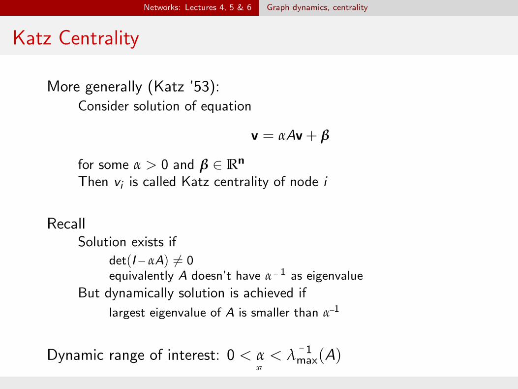
Katz Centrality
More generally (Katz ’53): Consider solution of equation
v = aAv + b
for some a > 0 and b 2 Rn
Then vi is called Katz centrality of node i
Recall Solution exists if
det(I – aA) 6= 0equivalently A doesn’t have a – 1
as eigenvalue But dynamically solution is achieved if
largest eigenvalue of A is smaller than a–1
1Dynamic range of interest: 0 < a < l (A)max37
–

��
���
�
Networks: Lectures 4, 5 & 6 Graph dynamics, centrality
PageRank
Goal: assign “importance” to each web-page in WWW Utilize it to order pages for providing most relevant search results
An insight If a page is important, and it points to other page, it must be important But the influence of a page should not amplify with number of neighbors
Formalizing the insight: vi be importance of page i
vi = a  Aij vj /kj + b,
j
for some a > 0 and b 2 R
38

�
�
�
� � �
� �
��
Networks: Lectures 4, 5 & 6 Graph dynamics, centrality
PageRank
PageRank vector v is solution of
v = aAD–1v + b1,
where D = diag (ki ) and 1 is vector of all 1
Solution
v = b(I – aAD–1)–11
= b(I + aAD–1 + a 2(AD–1)2 + . . . ) 1
That is, PageRank of page i is sum of weighted paths in it’s neighborhood plus a constant
39

��
���
���
Networks: Lectures 4, 5 & 6 Graph dynamics, centrality
Hubs and Authority
Goal: assign importance to authors By utilizing whose papers are cited by whom
An additional insight A node is important if it points to other important node For example, a review article is useful if it points to important works
Two types of important nodes Authorities: nodes that are important due to having useful information Hubs: nodes that tell where important authorities are
40
��
�
�
Networks: Lectures 4, 5 & 6 Graph dynamics, centrality
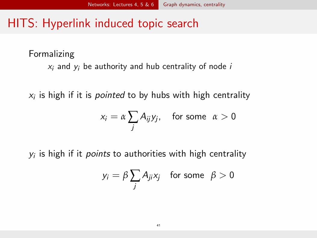
HITS: Hyperlink induced topic search
Formalizing xi and y
i be authority and hub centrality of node i
xi is high if it is pointed to by hubs with high centrality
xi = a ÂA
ij yj , for some a > 0j
yi is high if it points to authorities with high centrality
yi = b Â
j Aji xj for some b > 0
41
�
� �
���
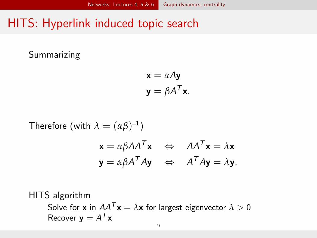
Networks: Lectures 4, 5 & 6 Graph dynamics, centrality
HITS: Hyperlink induced topic search
Summarizing
x = aAy
y = bAT x.
Therefore (with l = (ab)–1)
x = abAAT x , AAT
x = lxy = abAT Ay , AT Ay = ly.
HITS algorithm Solve for x in AAT
x = lx for largest eigenvector l > 0 Recover y = AT
x 42
�
���
���
Networks: Lectures 4, 5 & 6 Graph dynamics, centrality
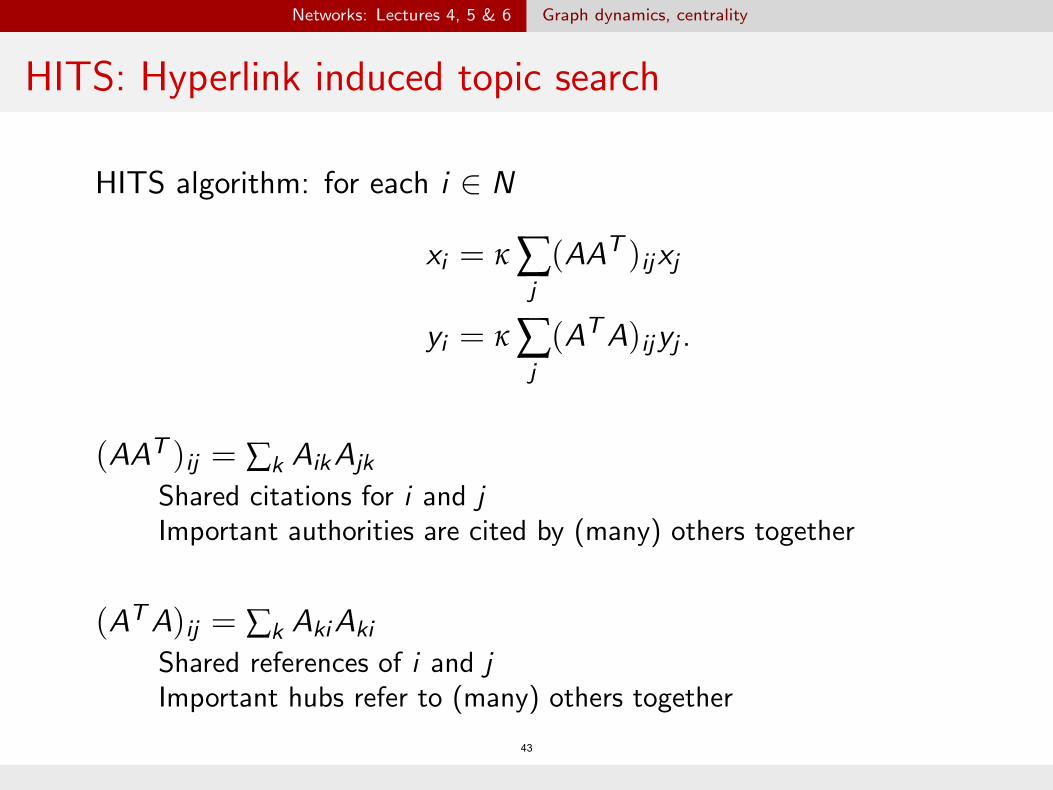
HITS: Hyperlink induced topic search
HITS algorithm: for each i 2 N
xi = k Â(AAT )
ij xjj
yi = k Â(AT A)
ij yj .j
(AAT )ij = Â
k Aik Ajk
Shared citations for i and j Important authorities are cited by (many) others together
(AT A)ij = Â
k Aki Aki
Shared references of i and j Important hubs refer to (many) others together
43

MIT OpenCourseWare https://ocw.mit.edu
14.15J/6.207J Networks Spring 2018
For information about citing these materials or our Terms of Use, visit: https://ocw.mit.edu/terms.