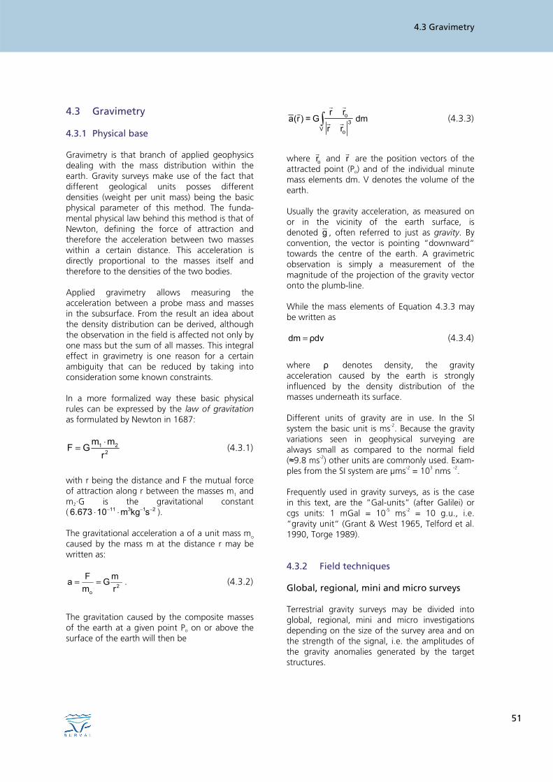
4.3 Gravimetry

51

4.3 Gravimetry

4.3.1 Physical base

Gravimetry is that branch of applied geophysics dealing with the mass distribution within the earth. Gravity surveys make use of the fact that different geological units posses different densities (weight per unit mass) being the basic physical parameter of this method. The funda-mental physical law behind this method is that of Newton, defining the force of attraction and therefore the acceleration between two masses within a certain distance. This acceleration is directly proportional to the masses itself and therefore to the densities of the two bodies. Applied gravimetry allows measuring the acceleration between a probe mass and masses in the subsurface. From the result an idea about the density distribution can be derived, although the observation in the field is affected not only by one mass but the sum of all masses. This integral effect in gravimetry is one reason for a certain ambiguity that can be reduced by taking into consideration some known constraints. In a more formalized way these basic physical rules can be expressed by the law of gravitation as formulated by Newton in 1687:

1 22

m mF G

r⋅

= (4.3.1)

with r being the distance and F the mutual force of attraction along r between the masses m1 and m2·G is the gravitational constant ( 11 3 1 26.673 10 m kg s− − −⋅ ⋅ ). The gravitational acceleration a of a unit mass mo caused by the mass m at the distance r may be written as:

2o

F ma Gm r

= = . (4.3.2)

The gravitation caused by the composite masses of the earth at a given point Po on or above the surface of the earth will then be

dmrr

rrG=)r(a

V3

o

o∫ rr

rr

(4.3.3)

where or

r and r

r are the position vectors of the

attracted point (Po) and of the individual minute mass elements dm. V denotes the volume of the earth. Usually the gravity acceleration, as measured on or in the vicinity of the earth surface, is denoted g , often referred to just as gravity. By convention, the vector is pointing “downward“ towards the centre of the earth. A gravimetric observation is simply a measurement of the magnitude of the projection of the gravity vector onto the plumb-line. While the mass elements of Equation 4.3.3 may be written as dm ρdv= (4.3.4)

where ρ denotes density, the gravity acceleration caused by the earth is strongly influenced by the density distribution of the masses underneath its surface. Different units of gravity are in use. In the SI system the basic unit is ms-2. Because the gravity variations seen in geophysical surveying are always small as compared to the normal field (≈9.8 ms-2) other units are commonly used. Exam-ples from the SI system are µms-2 = 103 nms -2. Frequently used in gravity surveys, as is the case in this text, are the “Gal-units” (after Galilei) or cgs units: 1 mGal = 10-5 ms-2 = 10 g.u., i.e. “gravity unit“ (Grant & West 1965, Telford et al. 1990, Torge 1989). 4.3.2 Field techniques

Global, regional, mini and micro surveys

Terrestrial gravity surveys may be divided into global, regional, mini and micro investigations depending on the size of the survey area and on the strength of the signal, i.e. the amplitudes of the gravity anomalies generated by the target structures.

STEEN THOMSEN & GERALD GABRIEL

52

Gravity surveys for mapping groundwater resources may be characterized as mini regarding the size of the survey area varying from some hundred metres to several kilometres, but as micro regarding the precision of the data to be obtained (Lakshmanan & Montlucon 1987, Reisz 1988, Thomsen 1988, 1990). Typically the anomaly amplitudes fall within the interval of a few tenths to a few hundreds µGal thus implying an accuracy of the gravity data better than 15 to 30 µGal. Gravimeters

Instruments for measuring gravity are called gravity meters, gravimeters or just meters. Gravimeters may be divided into absolute or relative instruments and into portable or stationary devices. While absolute gravimeters measure the absolute gravity, relative type meters measure only variations of the gravity field with time and space. Gravimeters for measuring the absolute gravity are not necessarily stationary, but they are rather complicated to move between different locations because of their size, weight and accessory equipments. Since relative type gravimeters are easier to handle and to carry, only this type is used for survey purposes in the frame of structural investigations. Around 1930 the first relative gravimeter based on the elastic spring concept was introduced. With the invention of the long-periodic vertical seismometer and the zero-length spring by L.J.B. LaCoste in 1934 the development towards improved sensitivity and portability of gravimeters gained. Actually the basic ideas of the most widely used gravimeters even today, with LaCoste & Romberg (LC&R) and to a minor extent Worden as prominent examples, are still the same. Because of instrument principles and design gravity observations have traditionally been performed as a manual process thus implying high demands of experience and competence by the observer. But since some 15 years automated gravimeters have been available. Under the name of Scintrex Autograv they come in different

models. As it is the case with every other gravimeters used for areal surveying, the sensing unit of Scintrex Autograv gravimeters is based on the elastic spring concept. Over the years the accuracies of gravimeters have been steadily enhanced. Modern gravimeters for areal surveying may under favourable field conditions produce data with accuracies in the interval 5 to 20 µGal. With the Scintrex CG-5 Autograv it is possible to produce data with a precision about 5–10 µGal. The LC&R model G meter can yield data with a precision in the interval 10–20 µGal depending on the field conditions and on the observer. Likewise with the LC&R model D meter data with a precision in the interval 5–15 µGal may be obtained. Both LC&R instruments may be equipped with an additional electronic feedback system thereby enhancing both the accuracy as well as reading procedure (Torge 1989). Survey area extension and data coverage

Preceding any gravimetric survey for mapping subsurface structures such as aquifers, the expected gravity signals have to be considered. Based on a priori information about geometry and density contrasts of the target structures possible signal amplitudes and frequency content should be estimated. Presupposed that the expected anomalies are of sufficient magnitude to be identified the survey area must be outlined. The area has to be large enough to reach well beyond the perimeter of the anomalies to be mapped. The individual measurement points of a gravity survey are traditionally denoted stations. Areal station (or data) coverage of the entire survey area is of course ideal since in this way 3-D modelling of the subsurface might then be accomplished. However, if the resources being available for a survey project are limited the question of a line-based survey may be relevant. Whether this alternative is appropriate should be evaluated while considering the expected shape of the subsurface target structures. When these can be

4.3 Gravimetry

53

approximated by 2-D models gravimetric traverses or profiles perpendicular across their supposed location might suffice. Often the actual outline of the station survey net is a compromise between geophysical requisites and economy. The result is in many cases a hybrid of the areal and the line type concepts. Such a hybrid net-design typically implies positioning stations primarily along roads and tracks while areal coverage may be restricted to urban districts. Based first of all on assumptions about the concrete geometry and depth of the target structures, the distance between the gravity stations has to be decided. General rules of thumb state that more shallow depth as well as shorter lateral extension of the targets implies shorter distances between stations. For ground water reservoir surveys distances between stations typically fall within the interval 50 to 300 metres. Definition of the gravity station net and localizing of the individual stations

Only gravimeters of the relative type are used for areal gravity surveys. Therefore the local net of survey stations should be tied to one or more stations of known absolute gravity in order to shift the observed gravity variations to absolute values. Only then the new data can be combined with existing data. Normally in the context of a given survey an absolute gravity station is characterized as the base- or a zero-order station. Preferably the gravity value should be given according to the International Gravity Standardization Net 1971, IGSN71, which is the current global gravity reference. Because of internal drift of the gravimeters field observations are normally carried out in measurement loops. A loop consists of a set of stations – typically 5 to 15 stations – of which the gravity of at least one, the reference station, is known. The first and the last gravity observation of a given loop should then be performed on the reference station while the rest of the stations are observed within the enclosed time interval. Gravity readings obtained during such a loop can hereby be corrected for instrumental drift and

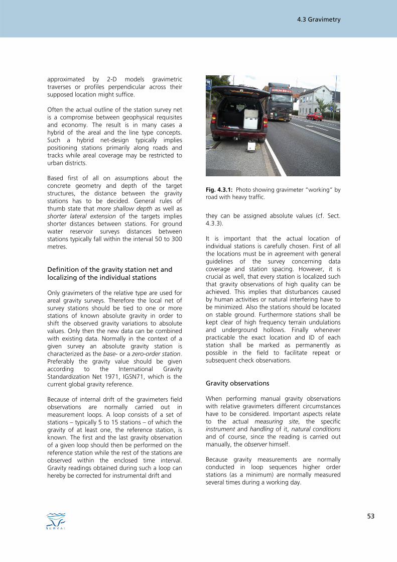
Fig. 4.3.1: Photo showing gravimeter “working” by road with heavy traffic.

they can be assigned absolute values (cf. Sect. 4.3.3). It is important that the actual location of individual stations is carefully chosen. First of all the locations must be in agreement with general guidelines of the survey concerning data coverage and station spacing. However, it is crucial as well, that every station is localized such that gravity observations of high quality can be achieved. This implies that disturbances caused by human activities or natural interfering have to be minimized. Also the stations should be located on stable ground. Furthermore stations shall be kept clear of high frequency terrain undulations and underground hollows. Finally whenever practicable the exact location and ID of each station shall be marked as permanently as possible in the field to facilitate repeat or subsequent check observations. Gravity observations

When performing manual gravity observations with relative gravimeters different circumstances have to be considered. Important aspects relate to the actual measuring site, the specific instrument and handling of it, natural conditions and of course, since the reading is carried out manually, the observer himself. Because gravity measurements are normally conducted in loop sequences higher order stations (as a minimum) are normally measured several times during a working day.

STEEN THOMSEN & GERALD GABRIEL

54

It is essential that the gravimeter is kept strictly levelled during each observation sequence. This requires continuous monitoring and frequent adjusting of the instrument level. The procedure associated with most manually operated gravimeters may be rather demanding with respect to time and mental concentration of the observer. Especially during hot summer days when stations are located on asphalt-paved ground this task are often really cumbersome and time-consuming while the “legs“ of the meter base “pan“ may slowly sink into the warm asphalt thereby distorting the measurements. Similar problems may arise if the underground is wet. With automatic gravimeters like the Scintrex CG-5 Autograv the problem of levelling the instrument are automatically handled by electronic tilt sensors. Along with automatic reading and logging of the data into the gravimeters memory measuring becomes less demanding as regards the involvement and skills of the observer. Positioning of the individual stations

Gravity is closely related to the actual position and height of observation (cf. Eq. 4.3.3 and Sect. 4.3.3). Therefore, it is of crucial importance for accurate gravimetric surveying to obtain precise data regarding the location of the individual gravity measurement points – the gravity stations. As a rule of thumb heights have to be known with a precision of 5 centimetres or better while errors on the latitude coordinates should not exceed 10 metres. Nowadays, these requirements can be achieved by using the Differential Global Positioning System. Possible (DGPS) errors on the longitude coordinates do not have consequences regarding gravity (cf. Sect. 4.3.3). With the introduction of the DGPS method the resources needed for positioning of gravity stations have been significantly reduced – manpower as well as time. Moreover the preci-sion obtained is comparable or even better than the results achieved with traditional methods. DGPS in its current design however encompasses two intrinsic shortcomings: One is the lack of

ability for operation in areas (mostly forests or urban areas with high buildings) where the view of the sky is significantly reduced by obstacles consequently limiting the areal utilization of the method. The other drawback is the inherent requirement for operating simultaneously two receivers: a stationary “base“-receiver and a mobile “rover“-receiver. The logistics involved in managing the base-receiver concurrently with the actual surveying may be considerable. 4.3.3 Data processing

Correction of gravity observations for temporal variations

Gravity does not only vary with location, but also with time. Celestial bodies such as the moon and the sun are the primary sources of temporal variations. The effect is denoted earth tides or just tides. The magnitude of earth tides can reach nearly ±150 μGal and therefore may be in the order of anomalies caused by the target structures. Moreover, gravity measurements vary with time because of instrumental reasons. This effect is normally denoted as gravimeter drift or just as drift. When the objective of gravity surveys as in the present context is to delineate underground (static) geological structures such as aquifers, gravity observations must be corrected for temporal variations (e.g. Gabriel 2006a). Prior to correcting the observed data for temporal variations though the data must be converted to units of gravity, since in the field reports the data will, when obtained by manually operated gravimeters, be given in “instrument units“. This procedure is usually quite simple but may be a little elaborated if the data were obtained using a gravimeter with an active electronic feedback system. The first temporal-effect to be corrected for is the tides. This correction is carried out for each individual observation by use of algorithms based on comprehensive theoretical and empirical knowledge together with, of course, information about the time (including the date) of the observation as well as the 3-D coordinates of the location. When the absolute time is known with

4.3 Gravimetry

55

an accuracy better than 2 minutes and the 3-D position is known within the error limits required for applying the position related corrections (see below) the error on the tide correction will not exceed 1 µGal. As explained in Section 4.3.2 gravity observations are performed in “loops“ typically consisting of 5 to 15 stations of which the gravity of at least one is known. The initial measurement is carried out on a station of known gravity, the reference station of the actual loop. Observations of the remaining stations follow without delay with a concluding second observation of the reference station to close the loop. Frequently the drift correction is carried out by use of a simple linear drift model

ref 2 ref1D i

2 1

g gΔg (i) tt t

−= ⋅−

(4.3.5)

where DΔg (i) is the drift correction on the i'th observation, ref1g and ref 2g are the observations on the reference station at times 1t and 2t while

it is the elapsed time between 1t and the i'th observation. When assuming the relative time of each observation is known with an accuracy better than 5 minutes, tide corrections have been applied prior to the drift correction, drift is smooth with no jumps and less than 100 µGal/day, and finally 2t – 1t <100 minutes, then the drift correction is assessed to be better than 1 µGal. The relative gravity values of a loop corrected for temporal variations are via the reference station with known gravity shifted to an absolute level

Abs ref,Abs Tide Dg (i) g (Δg(i,ref ) Δg (i) Δg (i))= + − − (4.3.6)

where Absg (i) is the absolute gravity at the location of the i'th observation, ref,Absg is the absolute gravity at the reference station, Δg(i,ref ) is the uncorrected observed gravity difference between the absolute gravity at the reference station and the location i while

TideΔg (i) and DΔg (i) are the tide respectively the drift correction of the i'th observation.

Bouguer anomaly and corrections related to position

As mentioned above gravity varies with location in space. The primary sources of variations of the earth gravity as measured on or close to its surface are related to the shape and rotation of the planet. Only a minute fraction of these variations is caused by density variations within the earth crust. With the aim to relatively amplify gravity signals bearing information about geological structures of the earths crust, the concept of the Bouguer anomaly was introduced (after the French mathematician Pierre Bouguer). In some cases also the free air anomaly is used in practise. The Bouguer anomaly is defined as

B Abs γ FA BP Topog g g g g g= − − − − (4.3.7)

and the free air anomaly as

F Abs γ FAg g g g= − − (4.3.7a)

where Bg is the Bouguer anomaly, Fg the free air anomaly, Absg the absolute gravity, γg the normal gravity, FAg the free air reduction, BPg the Bouguer plate reduction, and Topog the terrain correction. By subtracting the latter four components from the absolute gravity the remaining Bouguer anomaly reflects in a simplified sense solely the effect caused by density anomalies below the height reference surface, assuming that densities used in Equation 4.3.7 for the rocks between the station height and the reference surface are homogenous and correct (see below); for a detailed discussion see Ervin (1977), Hinze (1990) or Li & Götze (2001).

STEEN THOMSEN & GERALD GABRIEL

56

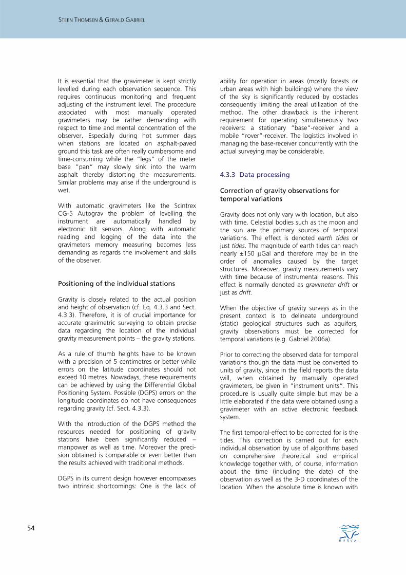
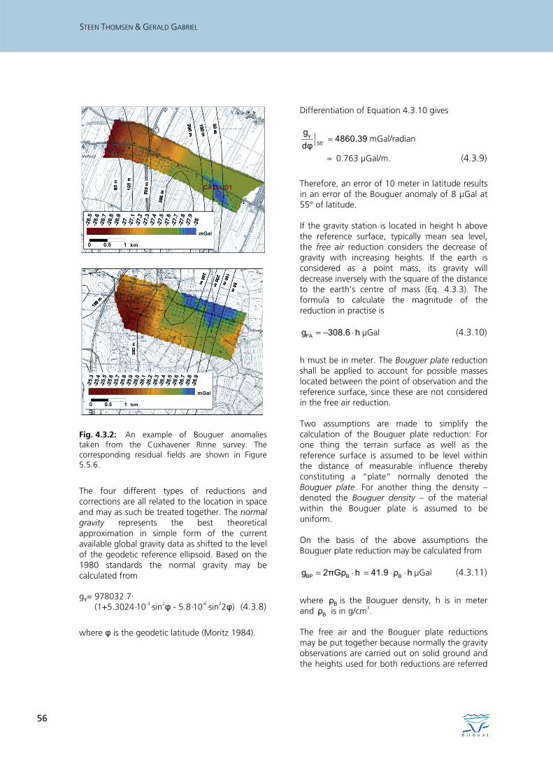
Fig. 4.3.2: An example of Bouguer anomalies taken from the Cuxhavener Rinne survey. The corresponding residual fields are shown in Figure 5.5.6.

The four different types of reductions and corrections are all related to the location in space and may as such be treated together. The normal gravity represents the best theoretical approximation in simple form of the current available global gravity data as shifted to the level of the geodetic reference ellipsoid. Based on the 1980 standards the normal gravity may be calculated from gγ= 978032.7· (1+5.3024·10-3·sin2φ - 5.8·10-6·sin22φ) (4.3.8)

where φ is the geodetic latitude (Moritz 1984).

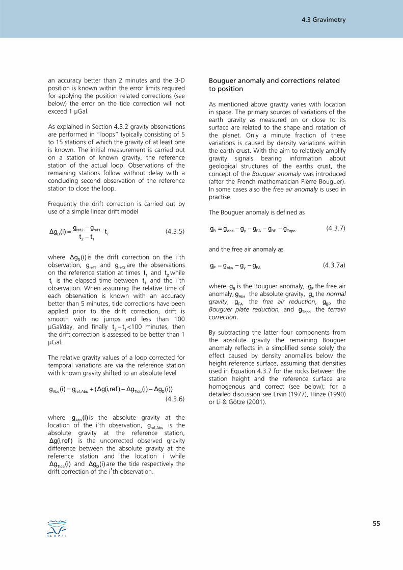
Differentiation of Equation 4.3.10 gives

γ55

g4860.39

dφ≈o mGal/radian

≈ 0.763 µGal/m. (4.3.9)

Therefore, an error of 10 meter in latitude results in an error of the Bouguer anomaly of 8 µGal at 55° of latitude. If the gravity station is located in height h above the reference surface, typically mean sea level, the free air reduction considers the decrease of gravity with increasing heights. If the earth is considered as a point mass, its gravity will decrease inversely with the square of the distance to the earth’s centre of mass (Eq. 4.3.3). The formula to calculate the magnitude of the reduction in practise is

FAg 308.6 h= − ⋅ µGal (4.3.10)

h must be in meter. The Bouguer plate reduction shall be applied to account for possible masses located between the point of observation and the reference surface, since these are not considered in the free air reduction. Two assumptions are made to simplify the calculation of the Bouguer plate reduction: For one thing the terrain surface as well as the reference surface is assumed to be level within the distance of measurable influence thereby constituting a “plate“ normally denoted the Bouguer plate. For another thing the density – denoted the Bouguer density – of the material within the Bouguer plate is assumed to be uniform. On the basis of the above assumptions the Bouguer plate reduction may be calculated from

BP Bg 2πGρ h= ⋅ B41.9 ρ h= ⋅ ⋅ µGal (4.3.11)

where Bρ is the Bouguer density, h is in meter and Bρ is in g/cm3. The free air and the Bouguer plate reductions may be put together because normally the gravity observations are carried out on solid ground and the heights used for both reductions are referred

4.3 Gravimetry

57

to the same reference surface. Of course if for instance a station by some reason is located on a bridge the situation is different. Therefore, when the Bouguer density has been chosen the free air and the Bouguer plate reductions are both solely depending on the height h of the measuring point. The combination of the two, sometimes referred to as the height reduction, may then be defined as (Dobrin 1981, p. 419)

Height FA BPg g g= + (4.3.12)

When the Bouguer density is set at 2000 kg/m3 (which for surveys in an area dominated by unconsolidated sediments like in Denmark has proved to be realistic) the height reduction can be calculated from

Heightg 224.5 h= − ⋅ µGal (4.3.13)

h is given in meter. Equation 4.3.13 indicates that an error of 5 centimetres will produce an error on the corrected gravity of 11 µGal. The purpose of the terrain correction is to account for the influence of an undulating topography within the distance of significant measurable gravity influence. For instance a nearby hill extending above the height of observation will erroneously reduce the gravity at the station because of the gravitational attraction of the hill exerts an upward component of gravity counteracting the pull from the rest of the earth. In the same way valleys extending below the height of the observation site will reduce the vertical component of the pull of the earth as measured on the station. Normally terrain corrections are quite complicated to calculate in practice, but whenever digital models of the terrain in question exist computer software may be applied. The magnitude of the terrain correction will increase with roughness of the landscape and with proximity of topographic features in regard to the individual gravity stations. Furthermore the correction is directly proportional to the density of the rocks constituting the surrounding terrain.

Investigations show that in regions of rather subdued topography like in Denmark the terrain correction may reach above 350 µGal. However the mean level of the correction of the major part of the country amounts some 15 µGal or less. Whether terrain corrections shall be applied depends on the roughness of the terrain and on the precision requirements of the survey. The correction may be estimated with an accuracy better than 20% depending primarily on the resolution and quality of the terrain model as well as on the actual location of the stations (Hamelmann & Snopek 2004, Thomsen 1988). Review on errors on gravity observations and corrections

Based on the above description of a worst-case total error estimate for the Bouguer anomaly results Be can be summarized as

B Obs Topoe e 1 1 8 11 e= + + + + + µGal

Obs Topo21 e e= + + µGal (4.3.14)

As described above the terms Obse and Topoe may vary considerably depending on type of gravimeter and terrain (cf. Sect. 4.3.2). However, under the assumption that the instrument used is LC&R model G gravimeter or better and that the corrections for the terrain – which is assumed to be subdued – effect has been applied, worst-case estimates of the two will be 20 µGal respectively 3 µGal. This leads to a worst-case total error estimate of 44 µGal. However, when a station has been observed more than once Obse will decrease with 1/ n where n is the number of observations. Moreover, when DGPS has been used for positioning, the error on the normal gravity γe will reduce to less than 50 nGal because the accuracy of the latitude coordinate will then be better than 3 centimetres. In other words: Under the above assumptions with each station observed at least twice the worst-case total error estimate on the Bouguer anomaly Be reduces to some 30 µGal. A conservative estimate of the mean total error may then be less than 20 µGal.

STEEN THOMSEN & GERALD GABRIEL

58

Assessing density magnitudes

In gravimetric surveys, density of the underground geology and surrounding terrain is a key physical parameter. On the one hand mapping the density distribution of the subsurface geology frequently constitutes an important part of the purpose of gravity surveys. On the other hand this requires a Bouguer or a free air anomaly version of the surveyed gravity field, which has to be calculated from the raw observations by applying the various corrections (see above) based partly on information about density of the surrounding terrain and of the subsurface between the level of observation and the level of reference. Various concepts for assessing the magnitude of density exist. These range from merely extracting the data from literature over sample measurements to genuine in-situ surveys. In-situ surveys may be conducted as measurements on the terrain surface (typically for estimating the Bouguer density) or as measurements down through drill-holes or mine shafts with the aim to obtain knowledge about density variations needed in the modelling and interpretation process. While gravimeters can be used for measuring density on the terrain surface, active radioactive logging instruments are normally utilized when gauging density of the surrounding rocks down through boreholes (e.g Fricke & Schön 1999, Rider 1996, Serra 1984). 4.3.4 Modelling and interpretation /

which results can be expected

When the raw gravity observations from a gravity survey have been processed the work on modelling and interpretation of the obtained Bouguer- or free air anomaly values commences. Usually only certain parts of the underground are considered. Therefore, the first step of the process aims at identifying and extracting signals caused by relevant geological structures from the total corrected gravity field. The outcome of this process, normally referred to as regional-residual-separation, is dependent on the amount and quality of a priori knowledge about the

geological setting of the area in question as well as on skills and experiences of the person performing the separation. The actual modelling and interpretation of the subsurface geology are then carried out based on the extracted residual gravity field. There exist several different concepts for doing this and some of these will be considered below. Generally spoken, two circumstances influence the reliability of the resulting models and interpretations. For one thing the amount and quality as well as the diversity of available additional data are of crucial importance. For another thing, the degree of consistency between geology and density is of principal significance as well. Regional-residual separation / extracting relevant signals from the surveyed gravity field

The purpose of regional-residual separation is to separate elements of the gravity field representing regional geological structures and elements caused by local sources with the former of these normally assumed to be located at greater depth than the latter. The wavelength of the gravity signal from a given source increases with distance. Therefore, separation of signals caused by sources located at greater depth from signals caused by shallow sources may consist in dividing the “total“ gravity field into a long wave part representing regional sources and into a short wave part representing the local geology. Methods for separating gravity field data may be characterized as graphical or as numerical. Graphical approaches are based on graphic displays of the obtained Bouguer (or free air) anomaly values of a survey – in case of 1-D surveys as profiles and in case of 2-D surveys as contour maps. A line or a smooth graph approximating the long wave element of the “total“ gravity field is then sketched onto the 1-D profile figure whereupon the short wave, or residual, part of the gravity anomaly is found by subtracting the smooth long wave graph from the surveyed data. Reducing the degree of “smoothness“ of the graph approximating the

4.3 Gravimetry

59

regional field will cause the resulting residual field more strongly to reflect local sources and vice versa. Two prominent groups of numerical methods for extracting or separating relevant gravity signals are known as field continuation and filtering. Strictly spoken, field continuation can be regarded as a special type of gravity field filtering. The process of field continuation of gravity fields implies vertical shifting and re-calculation of a field known at one height level to a different level. Depending on the direction of the shift, either long- or short wavelength elements of the field are amplified. As for continuation methods, also traditional filtering of gravity fields is a mathematical operation performed on a digital copy of the data. By filtering a gravity field, predefined wavelength intervals are extracted from the “total“ field. The filter may be defined so that either the long or the short wavelength components of the field are allowed to pass. This type of filters is termed as either low or high pass. Since filtering is normally conducted in the frequency domain, a low pass filter allows for only frequencies below certain limit passing through while high pass filters lets only frequencies above a specific limit through. “Low” frequencies correspond to long wavelengths, obviously, and “high“ frequencies correspond to short wavelength intervals. A special variety of digital filters is known as band pass. This type utilizes two limits – a “low“ and a “high“ threshold defining a frequency – or wavelengths – band within which signals passes through while frequencies outside are blocked. Most frequently, gravity data are obtained at varying distances throughout the survey area. Therefore, interpolation of the data to be defined at uniform spatial intervals must to be carried out since digital filtering cannot be performed on irregularly spaced data. An example of 2-D filtering taken from the Cuxhavener Rinne survey is shown in Figure 5.5.6, the corresponding Bouguer anomalies are shown in Figure 4.3.2.

Qualitative interpretations

The process of regional-residual separation is actually representing a qualitative interpretation of geology and density distribution. General knowledge concerning geometry and density of regional deep-seated geological elements is utilized in the separation process. Qualitative interpretation of extracted residual fields may be performed as well. Relevant topics are often associated with mapping the lateral limits of shallow geological structures such as buried valleys or lateral locations of subsurface fault planes. Estimating maximum depth to gravity anomaly sources is another common issue for qualitative interpretation of residual Bouguer – or free air – anomaly fields. Although it is well known that the lateral resolution of ordinary gravity anomaly fields is normally quite high, different versions of the gradient of the field are often employed for facilitating qualitative interpretation, e.g., of the lateral extension of shallow gravity sources. Recently a method closely associated with horizontal gravity gradients termed maximum curvature has been introduced (Stadtler et al. 2003, Stadtler 2001). In some situations, this method appears to expose rather clearly the lateral limits of shallow geological structures like buried valleys. Several methods for estimating the maximum depth to gravity anomaly sources exist. The so-called Smith rules belong to this category (Smith 1959). Quantitative modeling and interpretation

Quantitative modeling of gravity anomalies involves fitting of model responses to measured residual anomaly data by adjusting geometry and density of subsurface gravity source models. Modeling the data may be conducted either as a forward or as an inverse operation. When satisfactory models have been found, they have to be interpreted into geological models. Both processes are critically dependent on the amount and quality of a priori information.

STEEN THOMSEN & GERALD GABRIEL

60

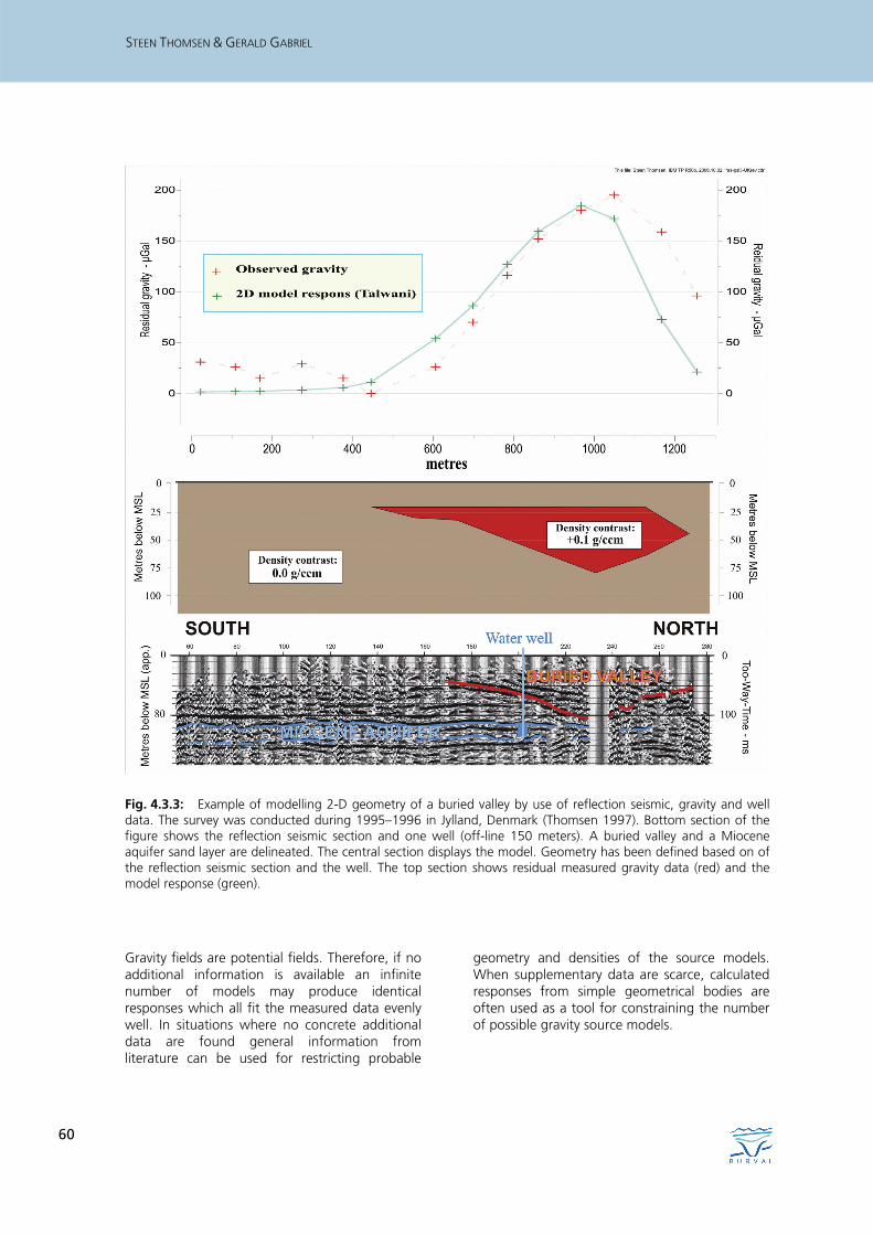
Fig. 4.3.3: Example of modelling 2-D geometry of a buried valley by use of reflection seismic, gravity and well data. The survey was conducted during 1995–1996 in Jylland, Denmark (Thomsen 1997). Bottom section of the figure shows the reflection seismic section and one well (off-line 150 meters). A buried valley and a Miocene aquifer sand layer are delineated. The central section displays the model. Geometry has been defined based on of the reflection seismic section and the well. The top section shows residual measured gravity data (red) and the model response (green).

Gravity fields are potential fields. Therefore, if no additional information is available an infinite number of models may produce identical responses which all fit the measured data evenly well. In situations where no concrete additional data are found general information from literature can be used for restricting probable

geometry and densities of the source models. When supplementary data are scarce, calculated responses from simple geometrical bodies are often used as a tool for constraining the number of possible gravity source models.

4.3 Gravimetry

61

More complex geometrical bodies, which approximate subsurface geology, are often established. Both 2-D and 3-D shaped bodies are considered. Since more than 40 years, a method for calculating the gravity response of 2-D polygon models – known as the Talwani formula – has been widely used (Talwani et al. 1959). Actually, Talwani’s formula has been implemented as the core algorithm for several computer programs calculating gravity effects of quite complex 2-D models. Several concepts for computing gravity effects of complex 3-D models have been developed over the passed three decades. One algorithm for calculating the response of arbitrary complex 3-D shaped bodies was presented by Götze & Lahmeyer (1988). Traditionally well information has been the prime source of independent information for modelling and interpreting gravity field data obtained for mapping aquifers. Well data may contribute important information on lithology and density as well as on the level of layer interfaces, thereby constraining the probable models in a point wise manner. However, since the last 10–15 years inclusion of reflection seismic data has been increasingly used as a mean for delineating 2-D geometry of the models. Figure 4.3.3 shows an example of modelling the 2-D geometry of a buried valley by use of reflection seismic, gravity and well data from a survey conducted close to the town of Skjern in Jylland, Denmark (Thomsen 1997). When geometry of the model has been established, the density contrasts may then be modelled by varying the contrasts until the model response fits the measured data. Further examples of forward modelling of buried valleys are found in Gabriel (2006b). A simple modelling concept involves approximating the depth interval of the subsurface which is supposed to span the sources of the residual gravity anomalies with a two-layer model. For this concept to work, the densities of the two layers must be individually relatively uniform and the contrast between the two has to be large enough to produce a detectable gravity signal. In the context of mapping aquifers, the idea of a two-layer model has been frequently utilized.

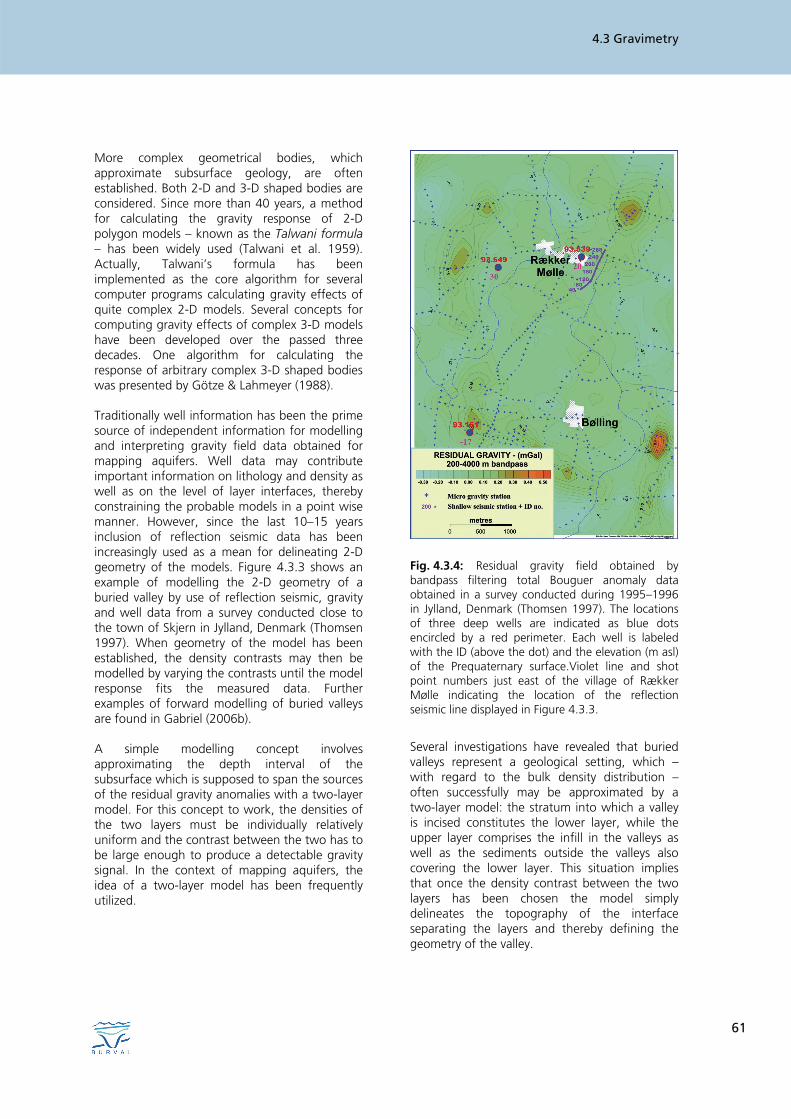
Fig. 4.3.4: Residual gravity field obtained by bandpass filtering total Bouguer anomaly data obtained in a survey conducted during 1995–1996 in Jylland, Denmark (Thomsen 1997). The locations of three deep wells are indicated as blue dots encircled by a red perimeter. Each well is labeled with the ID (above the dot) and the elevation (m asl) of the Prequaternary surface.Violet line and shot point numbers just east of the village of Rækker Mølle indicating the location of the reflection seismic line displayed in Figure 4.3.3.

Several investigations have revealed that buried valleys represent a geological setting, which – with regard to the bulk density distribution – often successfully may be approximated by a two-layer model: the stratum into which a valley is incised constitutes the lower layer, while the upper layer comprises the infill in the valleys as well as the sediments outside the valleys also covering the lower layer. This situation implies that once the density contrast between the two layers has been chosen the model simply delineates the topography of the interface separating the layers and thereby defining the geometry of the valley.

STEEN THOMSEN & GERALD GABRIEL

62

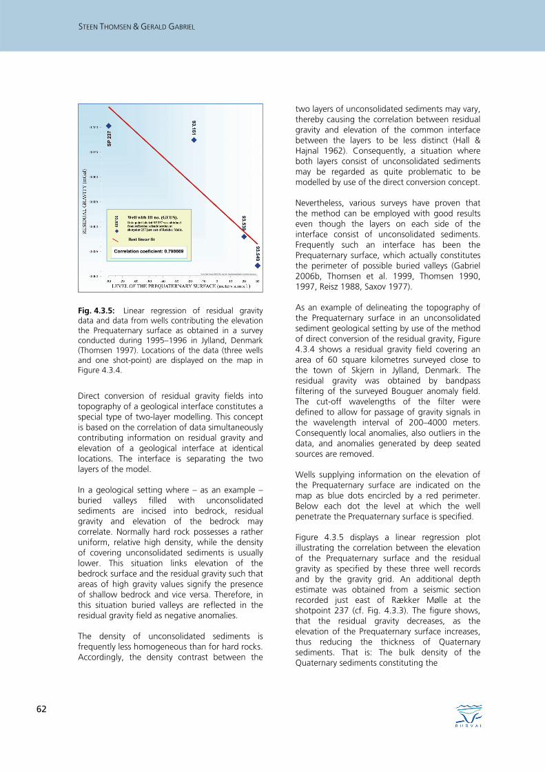
Fig. 4.3.5: Linear regression of residual gravity data and data from wells contributing the elevation the Prequaternary surface as obtained in a survey conducted during 1995–1996 in Jylland, Denmark (Thomsen 1997). Locations of the data (three wells and one shot-point) are displayed on the map in Figure 4.3.4.

Direct conversion of residual gravity fields into topography of a geological interface constitutes a special type of two-layer modelling. This concept is based on the correlation of data simultaneously contributing information on residual gravity and elevation of a geological interface at identical locations. The interface is separating the two layers of the model. In a geological setting where – as an example – buried valleys filled with unconsolidated sediments are incised into bedrock, residual gravity and elevation of the bedrock may correlate. Normally hard rock possesses a rather uniform, relative high density, while the density of covering unconsolidated sediments is usually lower. This situation links elevation of the bedrock surface and the residual gravity such that areas of high gravity values signify the presence of shallow bedrock and vice versa. Therefore, in this situation buried valleys are reflected in the residual gravity field as negative anomalies. The density of unconsolidated sediments is frequently less homogeneous than for hard rocks. Accordingly, the density contrast between the

two layers of unconsolidated sediments may vary, thereby causing the correlation between residual gravity and elevation of the common interface between the layers to be less distinct (Hall & Hajnal 1962). Consequently, a situation where both layers consist of unconsolidated sediments may be regarded as quite problematic to be modelled by use of the direct conversion concept. Nevertheless, various surveys have proven that the method can be employed with good results even though the layers on each side of the interface consist of unconsolidated sediments. Frequently such an interface has been the Prequaternary surface, which actually constitutes the perimeter of possible buried valleys (Gabriel 2006b, Thomsen et al. 1999, Thomsen 1990, 1997, Reisz 1988, Saxov 1977). As an example of delineating the topography of the Prequaternary surface in an unconsolidated sediment geological setting by use of the method of direct conversion of the residual gravity, Figure 4.3.4 shows a residual gravity field covering an area of 60 square kilometres surveyed close to the town of Skjern in Jylland, Denmark. The residual gravity was obtained by bandpass filtering of the surveyed Bouguer anomaly field. The cut-off wavelengths of the filter were defined to allow for passage of gravity signals in the wavelength interval of 200–4000 meters. Consequently local anomalies, also outliers in the data, and anomalies generated by deep seated sources are removed. Wells supplying information on the elevation of the Prequaternary surface are indicated on the map as blue dots encircled by a red perimeter. Below each dot the level at which the well penetrate the Prequaternary surface is specified. Figure 4.3.5 displays a linear regression plot illustrating the correlation between the elevation of the Prequaternary surface and the residual gravity as specified by these three well records and by the gravity grid. An additional depth estimate was obtained from a seismic section recorded just east of Rækker Mølle at the shotpoint 237 (cf. Fig. 4.3.3). The figure shows, that the residual gravity decreases, as the elevation of the Prequaternary surface increases, thus reducing the thickness of Quaternary sediments. That is: The bulk density of the Quaternary sediments constituting the

4.3 Gravimetry

63

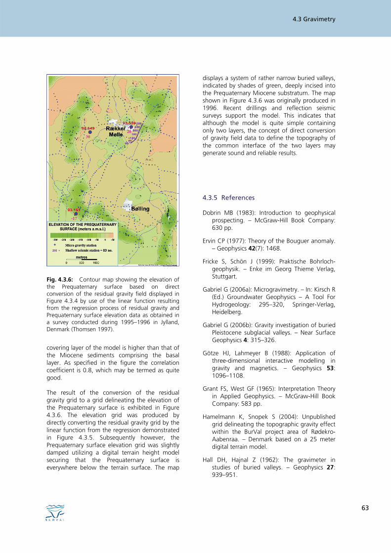
Fig. 4.3.6: Contour map showing the elevation of the Prequaternary surface based on direct conversion of the residual gravity field displayed in Figure 4.3.4 by use of the linear function resulting from the regression process of residual gravity and Prequaternary surface elevation data as obtained in a survey conducted during 1995–1996 in Jylland, Denmark (Thomsen 1997).

covering layer of the model is higher than that of the Miocene sediments comprising the basal layer. As specified in the figure the correlation coefficient is 0.8, which may be termed as quite good. The result of the conversion of the residual gravity grid to a grid delineating the elevation of the Prequaternary surface is exhibited in Figure 4.3.6. The elevation grid was produced by directly converting the residual gravity grid by the linear function from the regression demonstrated in Figure 4.3.5. Subsequently however, the Prequaternary surface elevation grid was slightly damped utilizing a digital terrain height model securing that the Prequaternary surface is everywhere below the terrain surface. The map

displays a system of rather narrow buried valleys, indicated by shades of green, deeply incised into the Prequaternary Miocene substratum. The map shown in Figure 4.3.6 was originally produced in 1996. Recent drillings and reflection seismic surveys support the model. This indicates that although the model is quite simple containing only two layers, the concept of direct conversion of gravity field data to define the topography of the common interface of the two layers may generate sound and reliable results. 4.3.5 References

Dobrin MB (1983): Introduction to geophysical prospecting. – McGraw-Hill Book Company: 630 pp.

Ervin CP (1977): Theory of the Bouguer anomaly. – Geophysics 42(7): 1468.

Fricke S, Schön J (1999): Praktische Bohrloch-geophysik. – Enke im Georg Thieme Verlag, Stuttgart.

Gabriel G (2006a): Microgravimetry. – In: Kirsch R (Ed.) Groundwater Geophysics – A Tool For Hydrogeology: 295–320, Springer-Verlag, Heidelberg.

Gabriel G (2006b): Gravity investigation of buried Pleistocene subglacial valleys. – Near Surface Geophysics 4: 315–326.

Götze HJ, Lahmeyer B (1988): Application of three-dimensional interactive modelling in gravity and magnetics. – Geophysics 53: 1096–1108.

Grant FS, West GF (1965): Interpretation Theory in Applied Geophysics. – McGraw-Hill Book Company: 583 pp.

Hamelmann K, Snopek S (2004): Unpublished grid delineating the topographic gravity effect within the BurVal project area of Rødekro-Aabenraa. – Denmark based on a 25 meter digital terrain model.

Hall DH, Hajnal Z (1962): The gravimeter in studies of buried valleys. – Geophysics 27: 939–951.

STEEN THOMSEN & GERALD GABRIEL

64

Hinze WJ (1990): The role of gravity and magnetic methods in engineering and environmental studies. – In: Ward SH (Ed.) Investigation of geophysics no. 5: Geotechnical and environmental geophysics (Vol. 1). Society of Exploration Geophysicists: 75–126.

Lakshmanan J, Montlucon J (1987): Microgravity probes the Great Pyramid. – The Leading Edge of Exploration 6(1): 10–17.

Li X, Götze HJ (2001): Ellipsoid, geoid, gravity, geodesy, and geophysics. – Geophysics 66(6): 1660–1668.

Moritz H (1984): Geodetic Reference System 1980. – Bulletin Géodésique 58: 388–398.

Reisz J (1988): Detailgravimetrisk kortlægning af Prækvartære dalstrøg syd for Århus. – Master Thesis, Aarhus Universitet, 117 pp.

Rider M (1996): The Geological Interpretation of Well Logs (2nd edn). – Whittles Publishing, Caithness.

Saxov S (1977): The application of gravimetry to groundwater exploration, with examples from Denmark and Sweeden. – Striae 4: 67–70, Uppsala.

Serra O (1984): Fundamentals of well log interpretation, Vol 1: the acquisition of logging data. – Dev. Pet. Sci., 15A, Elsevier, Amsterdam.

Smith, RA (1959): Some Depth Formulae for Local Magnetic and Gravity Anomalies. – Geophysical Prospecting 7(1): 55–63.

Stadtler C (2001): Mikrogravimetrische Untersuchungen im dänisch-deutschen Grenzgebiet. – Diplomarbeit, Ruhr-Universität Bochum: 100 pp.

Stadtler C, Casten U, Thomsen S (2003): Anwendung der “maximum curvature“ Methode auf Schweredaten zur Lokalisierung und Kartierung quartärer Rinnen in Südjütland (Dänemark). – Extended abstract GGP02, 63th Annual Meeting of the German Geophysical Society (DGG).

Talwani M, Worzel JL, Landisman M (1959): Rapid gravity computations for twodimensional bodies with application to the Mendocino submarine fracture zone. – Journal of Geophysical Research 64: 49–59.

Telford WM, Geldart LP, Sheriff RE (1990): Applied Geophysics (2nd edn). – Cambridge University Press: 770 pp.

Thomsen S (1988): Gravimetrisk undersøgelse i Vejle Ådal. – Master Thesis, Aarhus Universitet, 192 pp.

Thomsen S (1990): Surveying deepseated aquifers in Denmark. – Proceedings of the Eleventh Meeting of the Nordic Geodetic Comission, Copenhagen, 7.–11. May 1990: 526–538.

Thomsen S (1997): Kortlægning af dybtliggende grundvandsmagasiner i Danmark. – Afsluttende rapport. Sønderjyllands Amt & Kort- og Matrikelstyrelsen: 83 pp.

Thomsen S, Nørmark E, Lykke-Andersen H (1999): Buried valleys mapped by high-precision gravity and shallow seismic investigations. – Extended abstract 1, 61st EAGE Conference Helsinki 1999.

Torge W (1989): Gravimetry. – Walter de Gruyter: 465 pp.