Superconducting gravimetry at Onsala Space...
42
Superconducting gravimetry at Onsala Space Observatory The first year June 13, 2009 – Status August 31, 2010
Transcript of Superconducting gravimetry at Onsala Space...
Superconducting gravimetryat Onsala Space Observatory
The first year
June 13, 2009 –
Status August 31, 2010
Basic facts
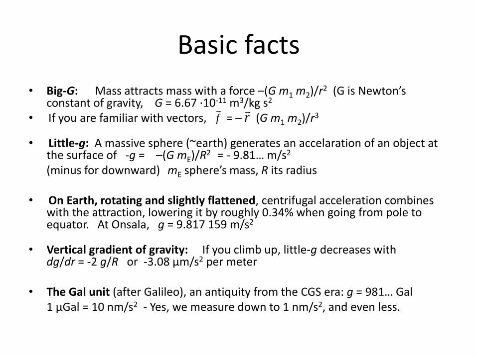
• Big-G: Mass attracts mass with a force –(G m1 m2)/r2 (G is Newton’sconstant of gravity, G = 6.67 ·10-11 m3/kg s2
• If you are familiar with vectors, = – (G m1 m2)/r3
• Little-g: A massive sphere (~earth) generates an accelaration of an object at the surface of -g = –(G mE)/R2 = - 9.81… m/s2
(minus for downward) mE sphere’s mass, R its radius
• On Earth, rotating and slightly flattened, centrifugal acceleration combineswith the attraction, lowering it by roughly 0.34% when going from pole to equator. At Onsala, g = 9.817 159 m/s2
• Vertical gradient of gravity: If you climb up, little-g decreases with dg/dr = -2 g/R or -3.08 µm/s2 per meter
• The Gal unit (after Galileo), an antiquity from the CGS era: g = 981… Gal1 µGal = 10 nm/s2 - Yes, we measure down to 1 nm/s2, and even less.
r
f
Gravimeters
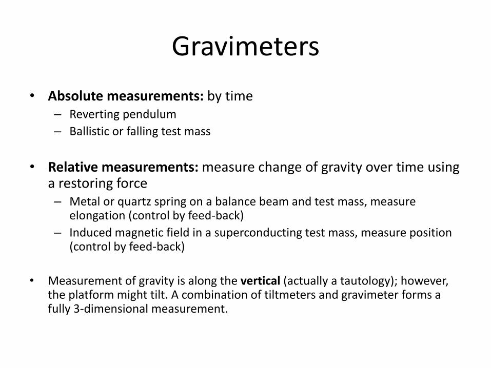
• Absolute measurements: by time– Reverting pendulum
– Ballistic or falling test mass
• Relative measurements: measure change of gravity over time usinga restoring force– Metal or quartz spring on a balance beam and test mass, measure
elongation (control by feed-back)
– Induced magnetic field in a superconducting test mass, measure position (control by feed-back)
• Measurement of gravity is along the vertical (actually a tautology); however, the platform might tilt. A combination of tiltmeters and gravimeter forms a fully 3-dimensional measurement.
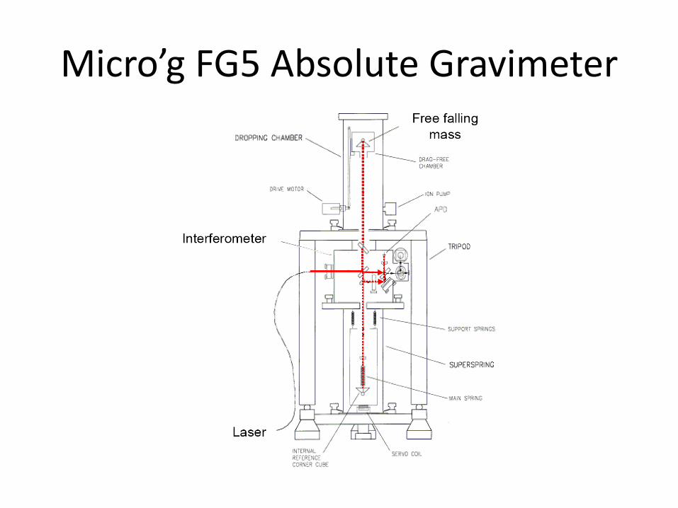
Micro’g FG5 Absolute Gravimeter
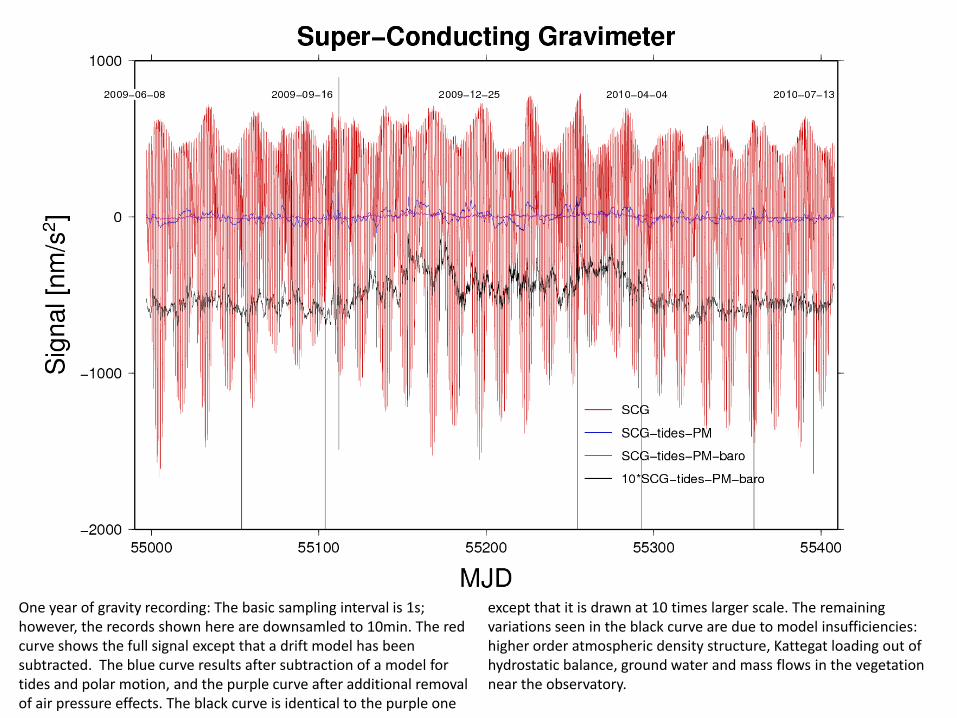
One year of gravity recording: The basic sampling interval is 1s; however, the records shown here are downsamled to 10min. The red curve shows the full signal except that a drift model has beensubtracted. The blue curve results after subtraction of a model for tides and polar motion, and the purple curve after additional removal of air pressure effects. The black curve is identical to the purple one
except that it is drawn at 10 times larger scale. The remainingvariations seen in the black curve are due to model insufficiencies: higher order atmospheric density structure, Kattegat loading out of hydrostatic balance, ground water and mass flows in the vegetation near the observatory.
One year of gravity recording: The basicsampling interval is 1s; however, the records shown here are downsamled to 10min. The red curve shows the full signal except that a drift model has beensubtracted. The blue curve results after subtraction of a model for tides and polar motion, and the purple curve after additional removal of air pressure effects.
The black curve is identical to the purpleone except that it is drawn at 10 timeslarger scale. The remaining variations seenin the black curve are due to modelinsufficiencies: higher order atmosphericdensity structure, Kattegat loading out of hydrostatic balance, ground water and mass flows in the vegetation near the observatory.
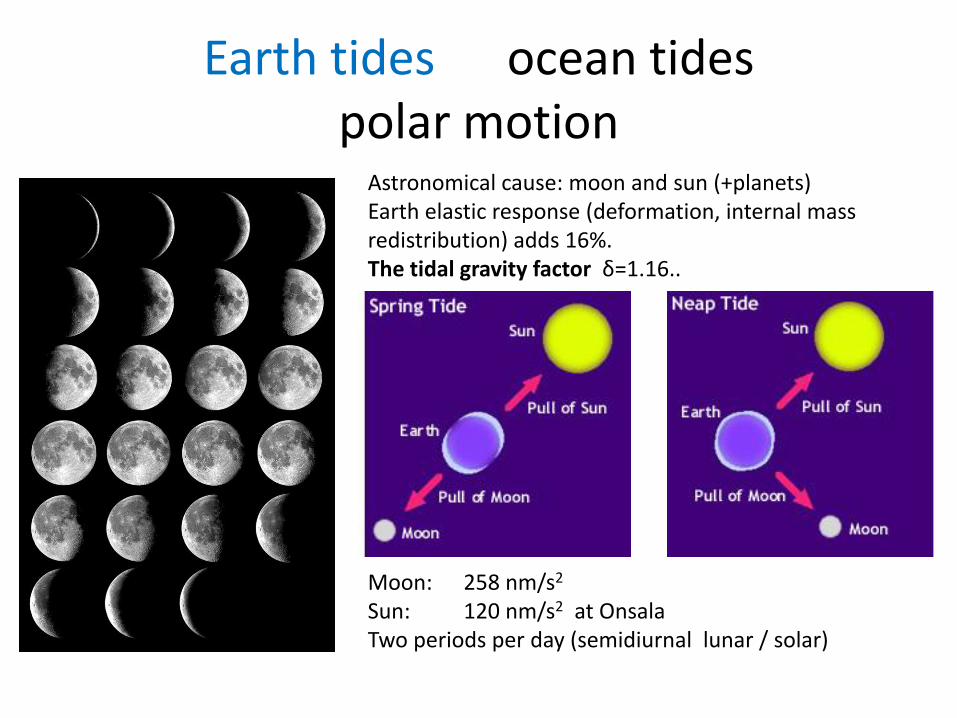
Earth tides ocean tidespolar motion
Astronomical cause: moon and sun (+planets)Earth elastic response (deformation, internal massredistribution) adds 16%. The tidal gravity factor δ=1.16..
Moon: 258 nm/s2
Sun: 120 nm/s2 at OnsalaTwo periods per day (semidiurnal lunar / solar)
• The Nearly-diurnal Free Wobble. The fluid core of the earth performs a free nutation around the earths rotation axis. The core rotates such that it makes one extra turn in 434 sidereal days. The resonance frequency of the nearly-diurnal free wobble, as the phenomenon is called, is thus(1/Ts) × (1+1/434)
• This motion implies pressure forces on the core-mantleboundary and internal mass redistribution. It affects the tidal gravity factor, lowering it from 1.16 to e.g. 1.14 at the K1 tide. And amplifying it at frequencies higher than the resonance frequency. The effect is narrow-banded and affects only diurnal tides.
Earth tides ocean tidespolar motion

Earth tides ocean tidespolar motion
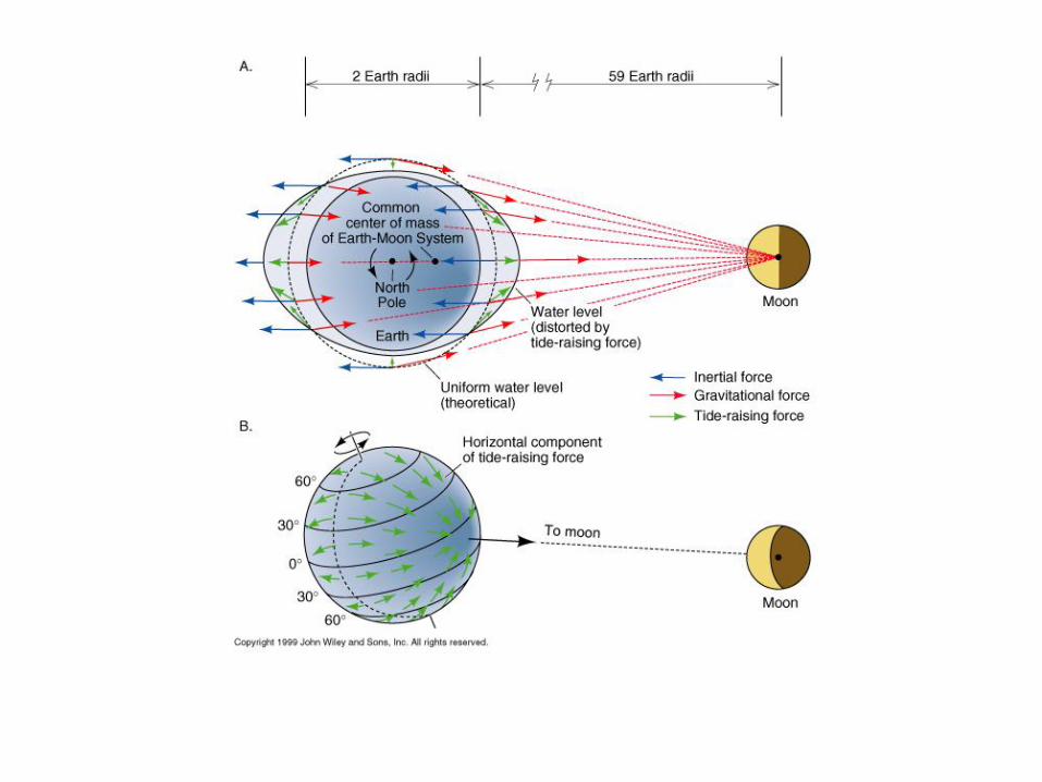
If moon and sun appeared only in the equatorial plane, we would not havebut semidiurnal tides, M2 (lunar) and S2 (solar).
The inclinations of the ecliptic and the lunar orbit cause the appearance of the bodies at different declinations aboveand below the equatorial plane during(solar, lunar) day and night, respectively. This gives rise to the diurnal tides, i.e. one period per (lunar, solar) day. The tide named K1 is suchan example (period = 1 sidereal day).
The tidal oscillation patterns in the oceans depend strongly on the periods of excitation.
Earth tides ocean tidespolar motion
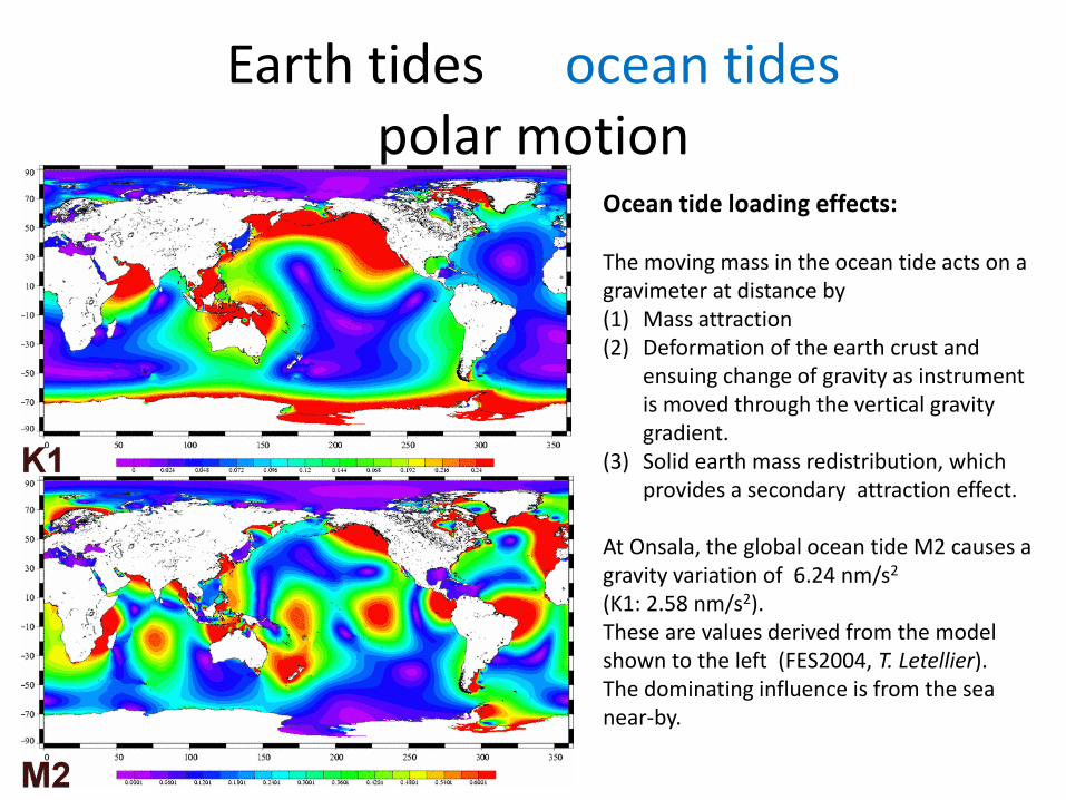
Ocean tide loading effects:
The moving mass in the ocean tide acts on a gravimeter at distance by(1) Mass attraction(2) Deformation of the earth crust and
ensuing change of gravity as instrument is moved through the vertical gravitygradient.
(3) Solid earth mass redistribution, whichprovides a secondary attraction effect.
At Onsala, the global ocean tide M2 causes a gravity variation of 6.24 nm/s2
(K1: 2.58 nm/s2). These are values derived from the modelshown to the left (FES2004, T. Letellier). The dominating influence is from the seanear-by.
Earth tides ocean tidespolar motion
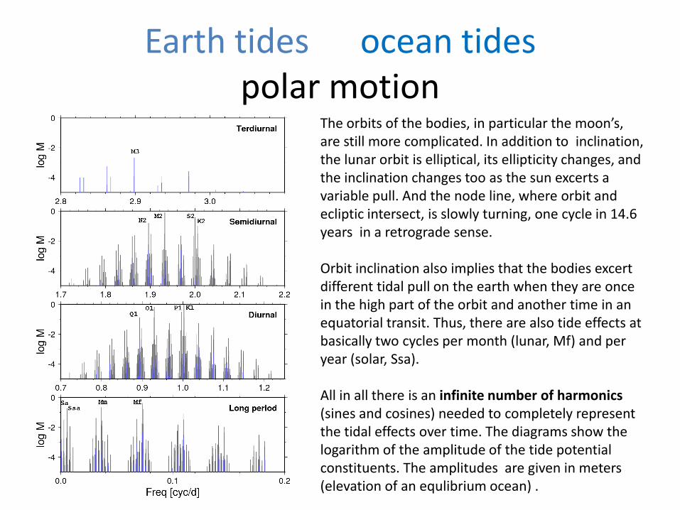
The orbits of the bodies, in particular the moon’s, are still more complicated. In addition to inclination, the lunar orbit is elliptical, its ellipticity changes, and the inclination changes too as the sun excerts a variable pull. And the node line, where orbit and ecliptic intersect, is slowly turning, one cycle in 14.6 years in a retrograde sense.
Orbit inclination also implies that the bodies excertdifferent tidal pull on the earth when they are oncein the high part of the orbit and another time in an equatorial transit. Thus, there are also tide effects at basically two cycles per month (lunar, Mf) and per year (solar, Ssa).
All in all there is an infinite number of harmonics(sines and cosines) needed to completely representthe tidal effects over time. The diagrams show the logarithm of the amplitude of the tide potential constituents. The amplitudes are given in meters (elevation of an equlibrium ocean) .
Earth tides ocean tidespolar motion
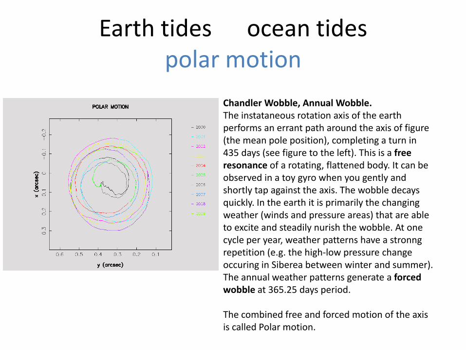
Chandler Wobble, Annual Wobble. The instataneous rotation axis of the earthperforms an errant path around the axis of figure(the mean pole position), completing a turn in 435 days (see figure to the left). This is a freeresonance of a rotating, flattened body. It can be observed in a toy gyro when you gently and shortly tap against the axis. The wobble decaysquickly. In the earth it is primarily the changingweather (winds and pressure areas) that are ableto excite and steadily nurish the wobble. At onecycle per year, weather patterns have a stronngrepetition (e.g. the high-low pressure changeoccuring in Siberea between winter and summer). The annual weather patterns generate a forcedwobble at 365.25 days period.
The combined free and forced motion of the axisis called Polar motion.
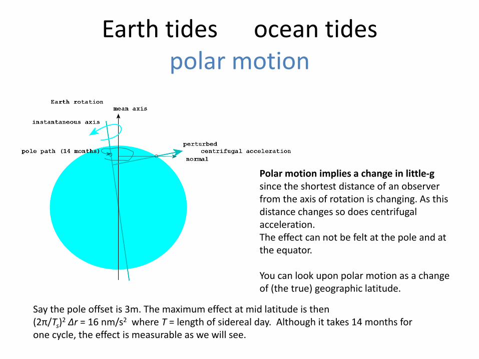
Earth tides ocean tidespolar motion
Polar motion implies a change in little-gsince the shortest distance of an observerfrom the axis of rotation is changing. As this distance changes so does centrifugal acceleration. The effect can not be felt at the pole and at the equator.
You can look upon polar motion as a changeof (the true) geographic latitude.
Say the pole offset is 3m. The maximum effect at mid latitude is then(2π/Ts)
2 Δr = 16 nm/s2 where T = length of sidereal day. Although it takes 14 months for one cycle, the effect is measurable as we will see.
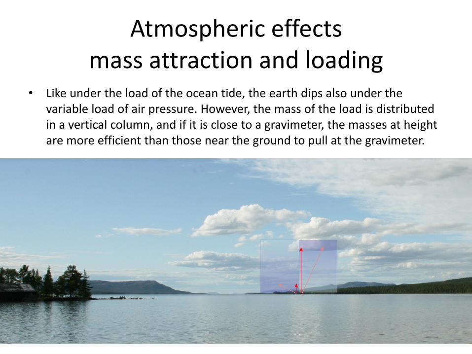
Atmospheric effectsmass attraction and loading
• Like under the load of the ocean tide, the earth dips also under the variable load of air pressure. However, the mass of the load is distributedin a vertical column, and if it is close to a gravimeter, the masses at heightare more efficient than those near the ground to pull at the gravimeter.
Hydrodynamic Loading
• Where air pressure acts on the ocean surface, the water adjusts so that the pressure at the ocean bottom remains constant. This is the so-calledinverse barometer effect. So, air pressure above ocean would not deformthe earth, although the sea level would change.
• However the ocean needs time to adjust. The shallower the water and the narrower the straights, the longer is the time for adjustment.
• Wind fields and fast travelling low-pressure systems excite oscillations in basins and pile up water at the coast.
• Thus, near the shores of shallow, semi-enclosed basins the sea level is in hydrostatic balance only on the time scale of days to weeks. The misadjustment causes loading and mass attraction.
Ground water and biosphere
• Variable ground water masses and the water cycle in the biosphere canimply mass changes in the very near environment of a gravimeter station. Especially ground water presents a serious problem if hydrology is considered a source of noise (while the measurement of ground water variations with a gravimeter is a clumsy and expensive method) .
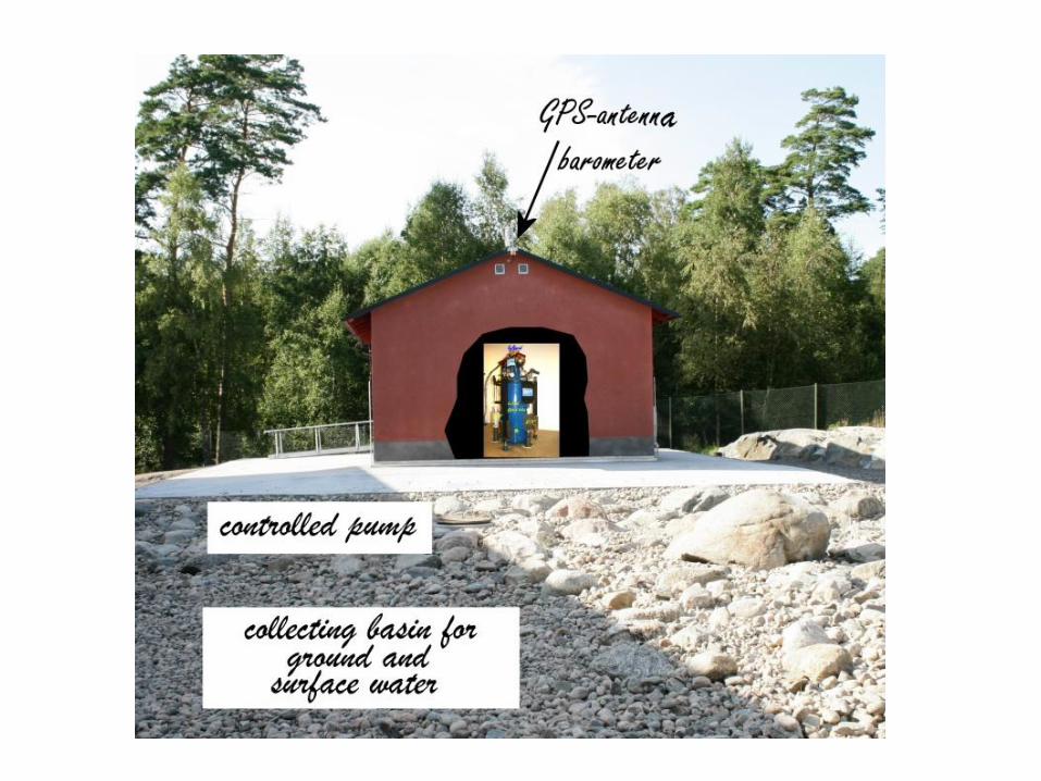
• The gravimeter lab at Onsala is situated on crystalline bedrock, which is expected to host small water masses. Precautions during constructionprevent the accumulation of rain water. It is collected in an underground pond and pumped away by controlling a constant water level in the pond.
• However, the forest (trees, undervegetation, soil) on the neighbourground is out of the observatory’s control. Here, we will have to deal with seasonal perturbations due mostly to the vegetation.
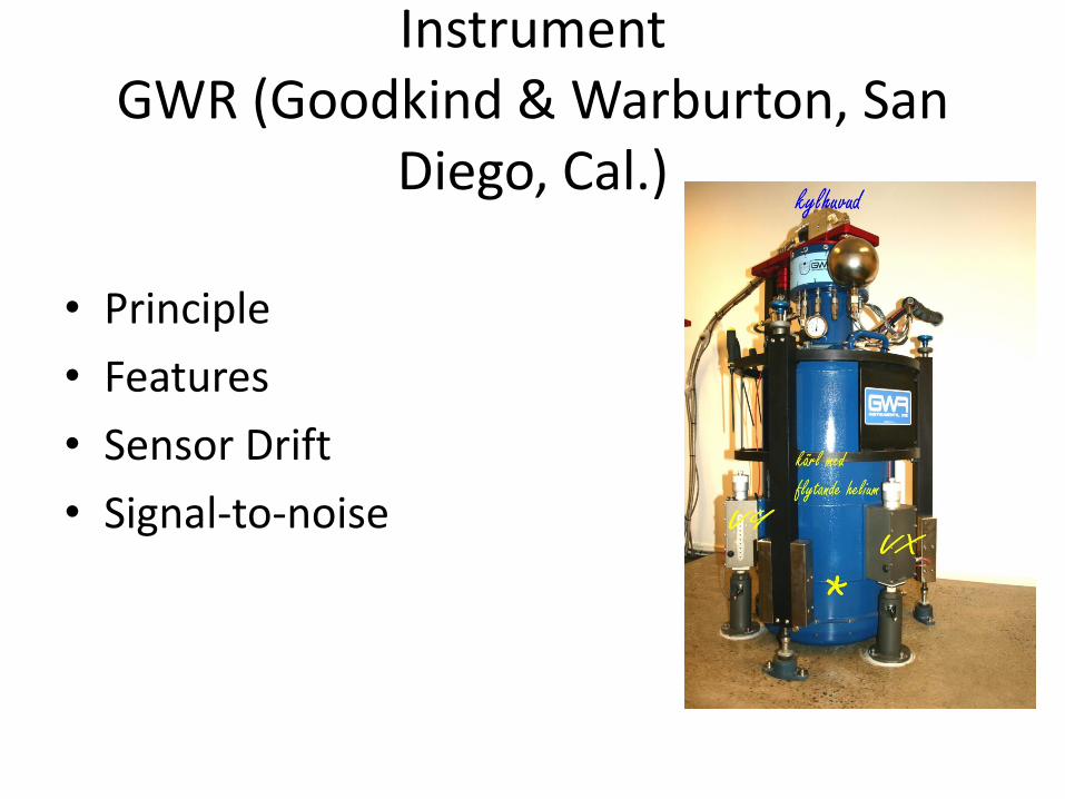
InstrumentGWR (Goodkind & Warburton, San
Diego, Cal.)
• Principle
• Features
• Sensor Drift
• Signal-to-noise
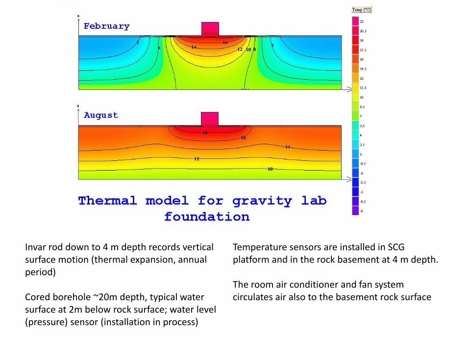
Invar rod down to 4 m depth records verticalsurface motion (thermal expansion, annualperiod)
Cored borehole ~20m depth, typical water surface at 2m below rock surface; water level(pressure) sensor (installation in process)
Temperature sensors are installed in SCG platform and in the rock basement at 4 m depth.
The room air conditioner and fan system circulates air also to the basement rock surface
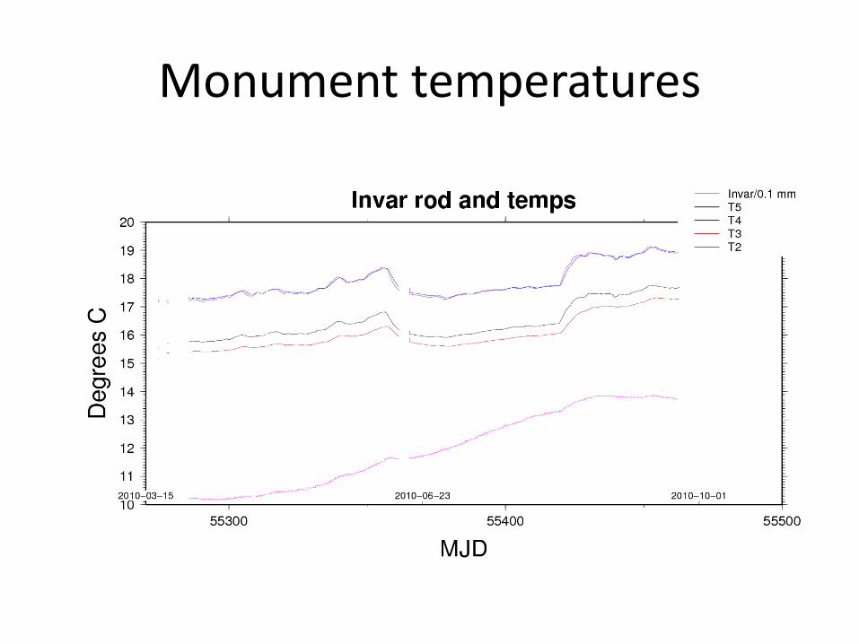
Monument temperatures
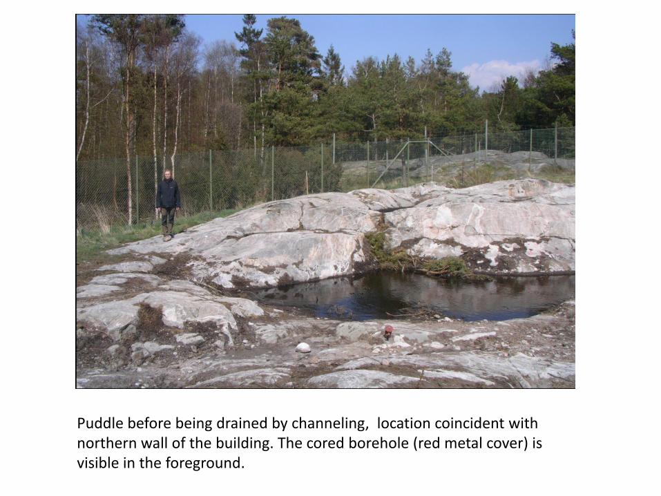
Puddle before being drained by channeling, location coincident with northern wall of the building. The cored borehole (red metal cover) is visible in the foreground.
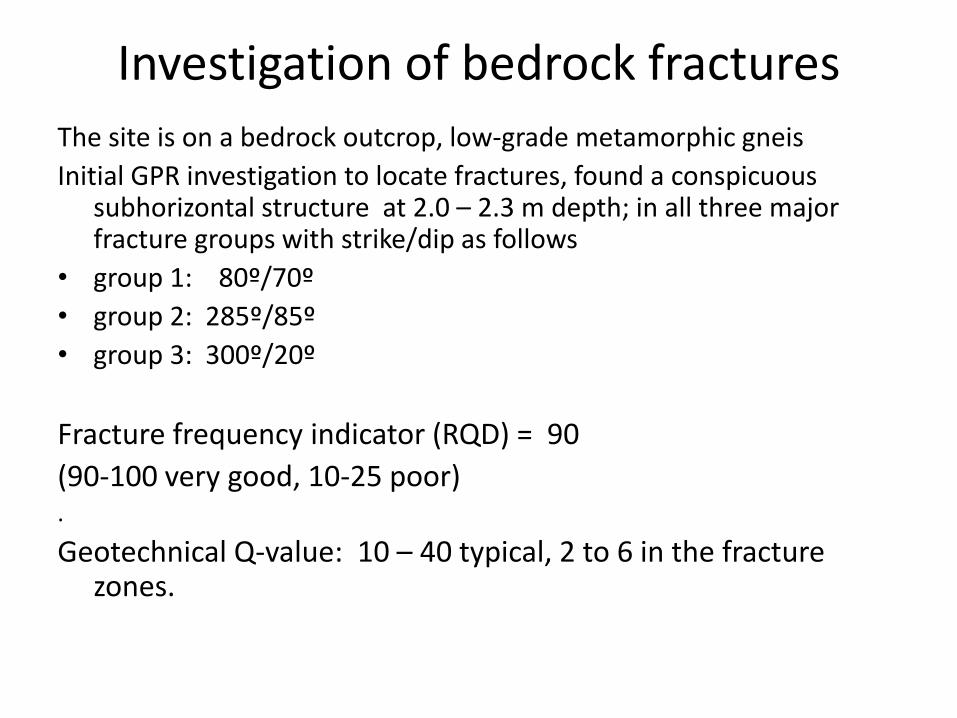
Investigation of bedrock fractures
The site is on a bedrock outcrop, low-grade metamorphic gneis
Initial GPR investigation to locate fractures, found a conspicuoussubhorizontal structure at 2.0 – 2.3 m depth; in all three major fracture groups with strike/dip as follows
• group 1: 80º/70º
• group 2: 285º/85º
• group 3: 300º/20º
Fracture frequency indicator (RQD) = 90
(90-100 very good, 10-25 poor).
Geotechnical Q-value: 10 – 40 typical, 2 to 6 in the fracturezones.
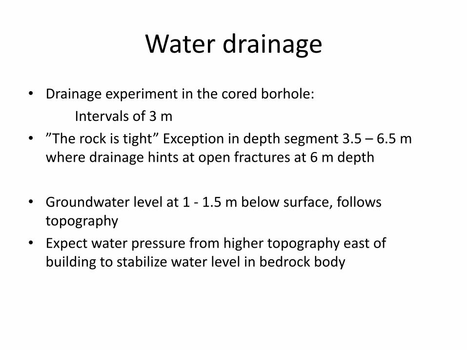
Water drainage
• Drainage experiment in the cored borhole:
Intervals of 3 m
• ”The rock is tight” Exception in depth segment 3.5 – 6.5 m where drainage hints at open fractures at 6 m depth
• Groundwater level at 1 - 1.5 m below surface, followstopography
• Expect water pressure from higher topography east of building to stabilize water level in bedrock body
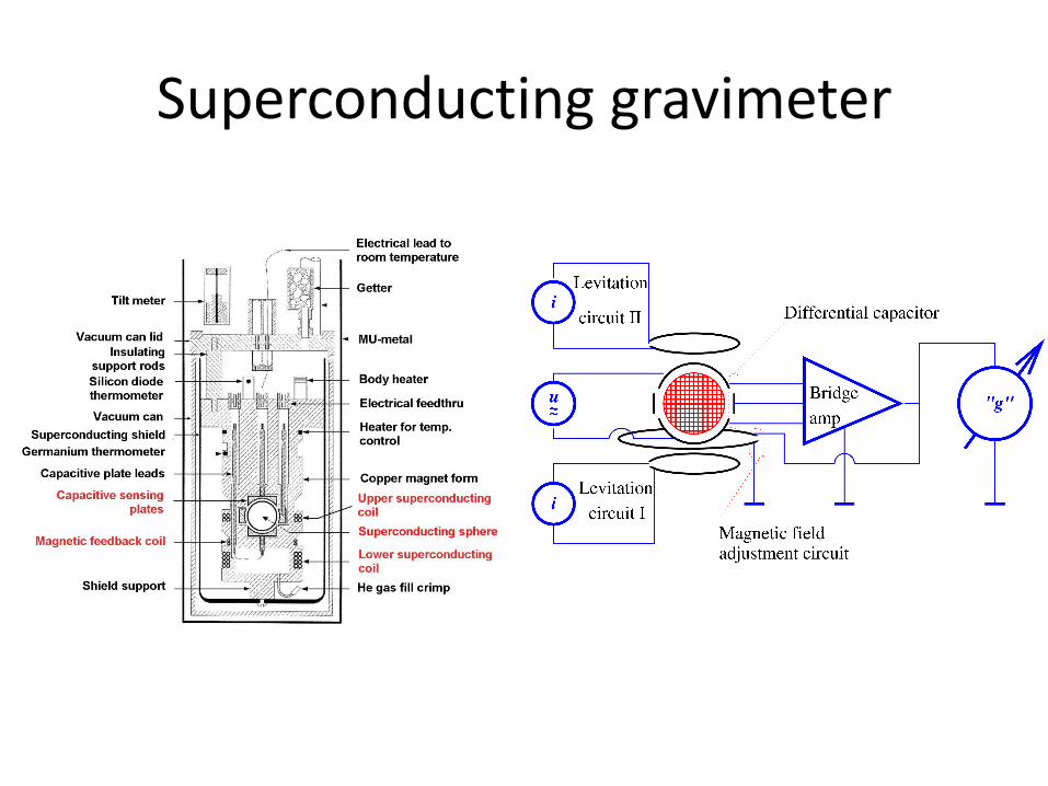
Superconducting gravimeter
• Cryogenic sensor
• Feedback loop
• Feedback controlled levelling
• 60 l liquid helium dewar
• Coldhead generates liquid from room-temperature He gas.
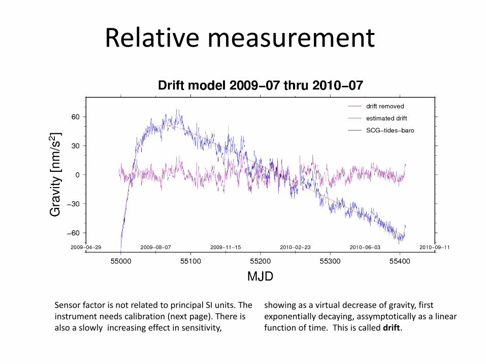
Relative measurement
Sensor factor is not related to principal SI units. The instrument needs calibration (next page). There is also a slowly increasing effect in sensitivity,
showing as a virtual decrease of gravity, first exponentially decaying, assymptotically as a linearfunction of time. This is called drift.
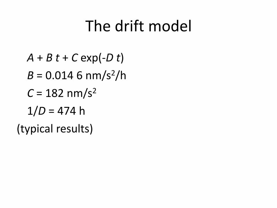
The drift model
A + B t + C exp(-D t)
B = 0.014 6 nm/s2/h
C = 182 nm/s2
1/D = 474 h
(typical results)
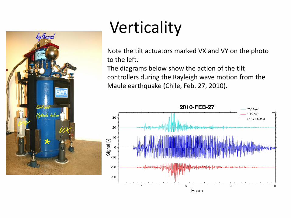
VerticalityNote the tilt actuators marked VX and VY on the phototo the left. The diagrams below show the action of the tiltcontrollers during the Rayleigh wave motion from the Maule earthquake (Chile, Feb. 27, 2010).
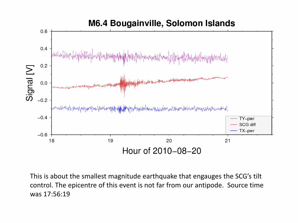
This is about the smallest magnitude earthquake that engauges the SCG’s tiltcontrol. The epicentre of this event is not far from our antipode. Source time was 17:56:19
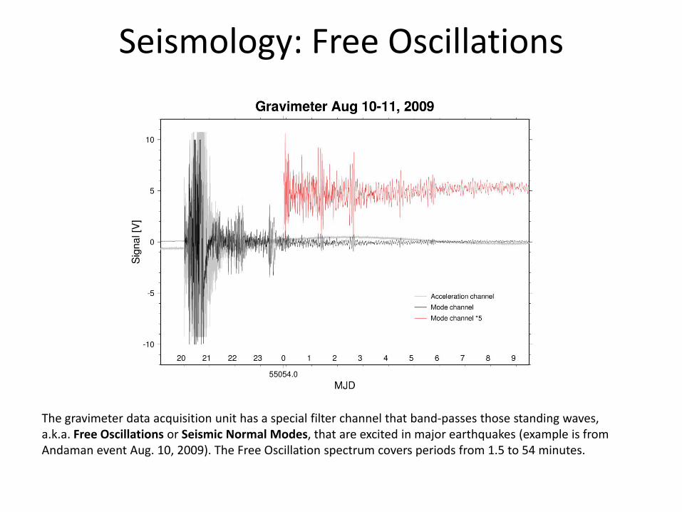
Seismology: Free Oscillations
The gravimeter data acquisition unit has a special filter channel that band-passes those standing waves, a.k.a. Free Oscillations or Seismic Normal Modes, that are excited in major earthquakes (example is from Andaman event Aug. 10, 2009). The Free Oscillation spectrum covers periods from 1.5 to 54 minutes.
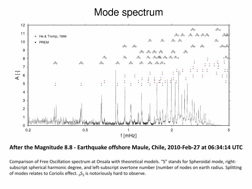
After the Magnitude 8.8 - Earthquake offshore Maule, Chile, 2010-Feb-27 at 06:34:14 UTC
Comparison of Free Oscillation spectrum at Onsala with theoretical models. “S” stands for Spheroidal mode, right-subscript spherical harmonic degree, and left-subscript overtone number (number of nodes on earth radius. Splitting of modes relates to Coriolis effect. 0S2 is notoriously hard to observe.
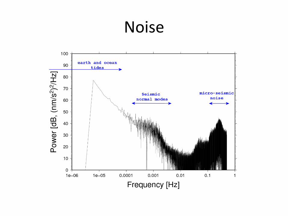
Noise
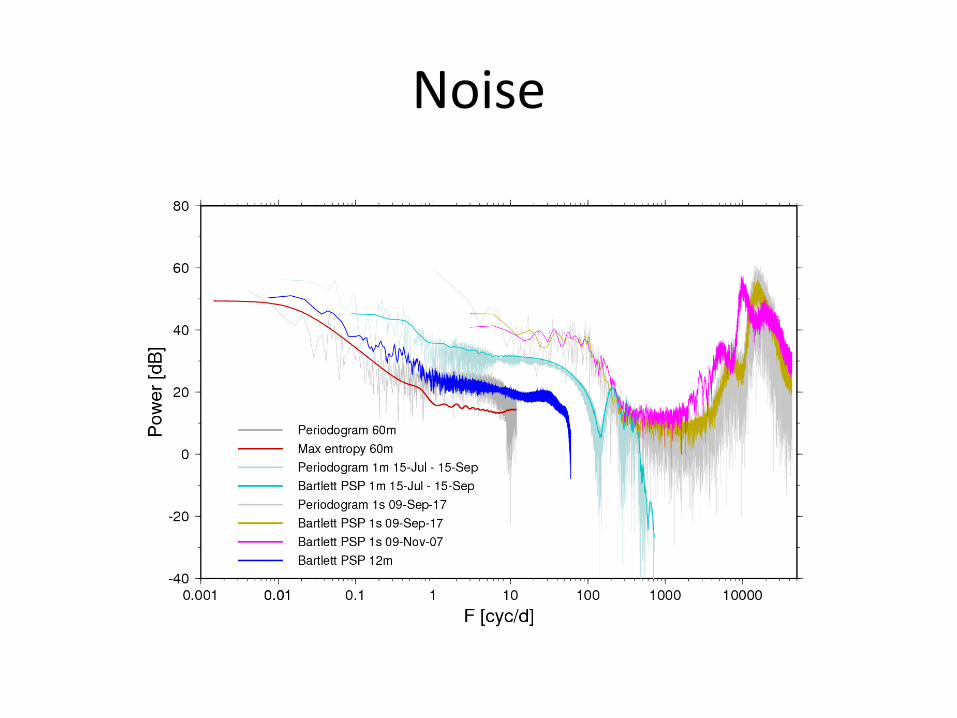
Noise
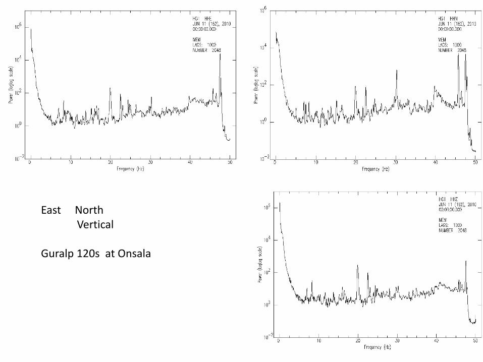
East NorthVertical
Guralp 120s at Onsala
GIA – glacial isostatic adjustment
• Research target for an AG project
• AG calibrates SCG
Isostasy = a solid body without internal forcesthat change its shape and gravity field.
GIA is the visco-elastic rebound after glacial loading and unloading. The earthreturns slowly to its pre-loading shape. Gravity anomaly (internal buoyancy) provides the force, visco-elasticity the resistance. The oceans with theirvariable mass adjust to the ambient gravity field and at the same time provides a dynamic load.
Peripheral to the uplifting dome is a subsiding trough, an effect of the elasticity of the lithosphere (top ~200 km of the earth). Ratio of central upliftversus peripheral subsidence ~10 : 1 (mm/yr) in and around Fennoscandia.
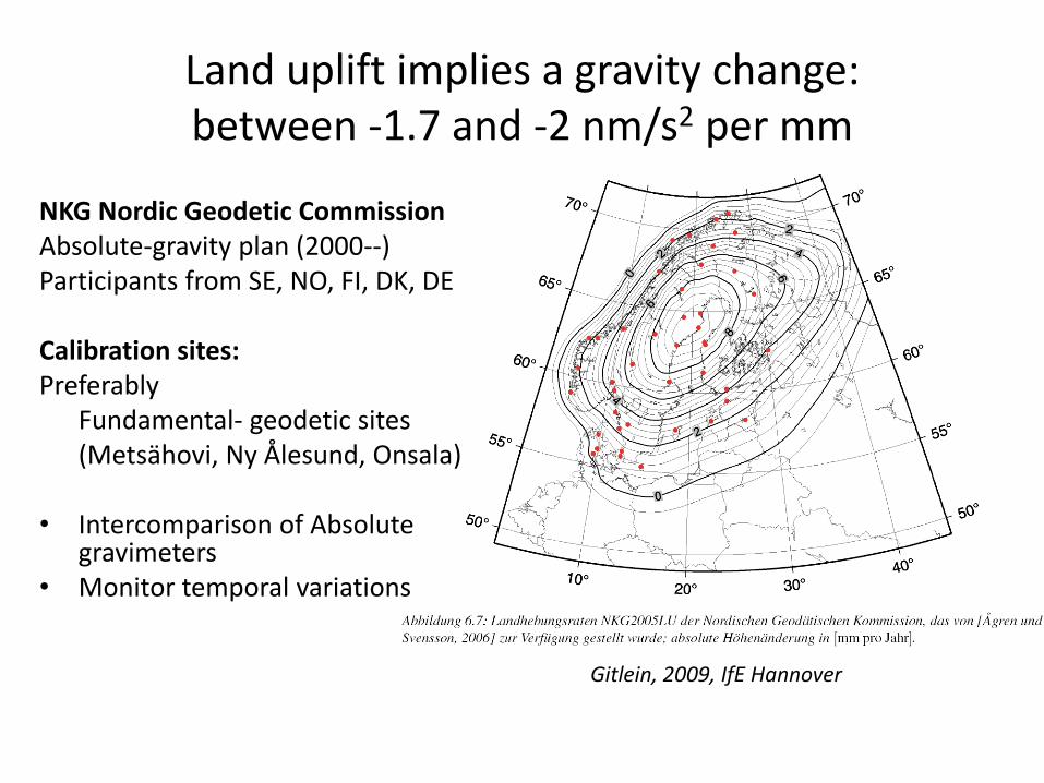
Land uplift implies a gravity change:between -1.7 and -2 nm/s2 per mm
NKG Nordic Geodetic CommissionAbsolute-gravity plan (2000--)Participants from SE, NO, FI, DK, DE
Calibration sites: Preferably
Fundamental- geodetic sites (Metsähovi, Ny Ålesund, Onsala)
• Intercomparison of Absolute gravimeters
• Monitor temporal variations
Gitlein, 2009, IfE Hannover
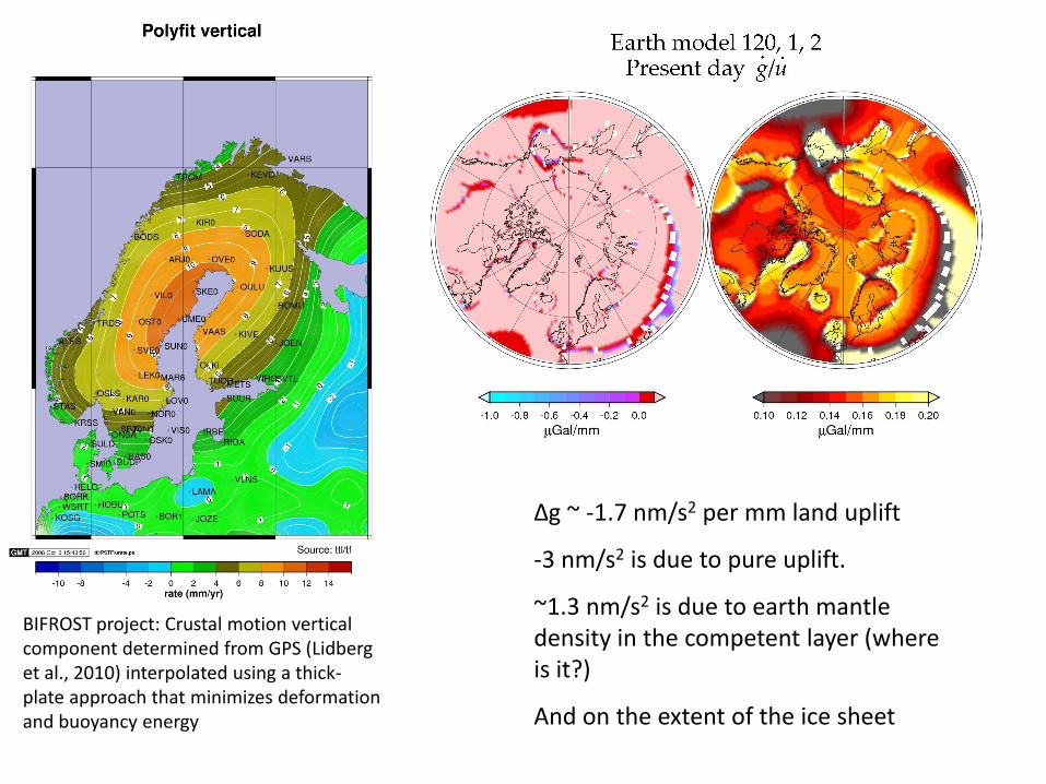
Δg ~ -1.7 nm/s2 per mm land uplift
-3 nm/s2 is due to pure uplift.
~1.3 nm/s2 is due to earth mantle density in the competent layer (where is it?)
And on the extent of the ice sheet
BIFROST project: Crustal motion verticalcomponent determined from GPS (Lidberg et al., 2010) interpolated using a thick-plate approach that minimizes deformation and buoyancy energy
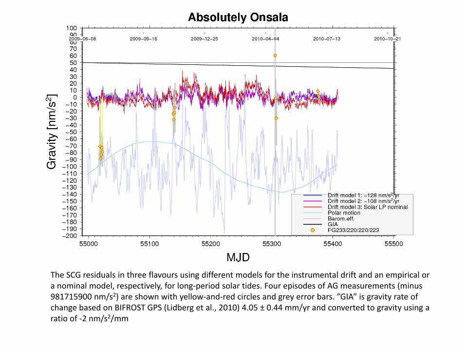
The SCG residuals in three flavours using different models for the instrumental drift and an empirical or a nominal model, respectively, for long-period solar tides. Four episodes of AG measurements (minus 981715900 nm/s2) are shown with yellow-and-red circles and grey error bars. ”GIA” is gravity rate of change based on BIFROST GPS (Lidberg et al., 2010) 4.05 ± 0.44 mm/yr and converted to gravity using a ratio of -2 nm/s2/mm
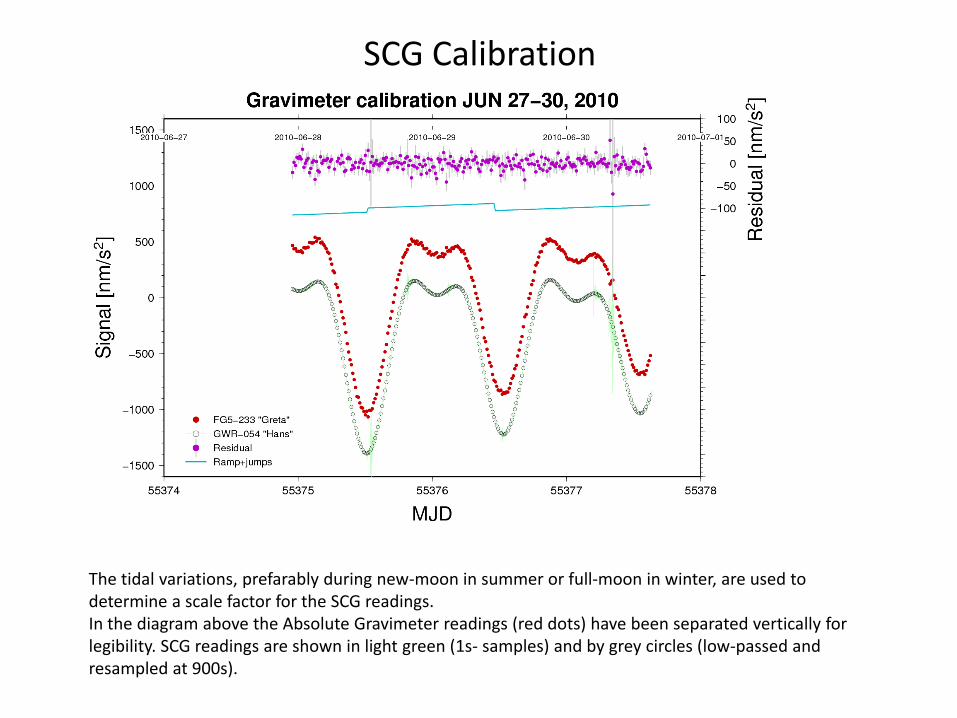
SCG Calibration
The tidal variations, prefarably during new-moon in summer or full-moon in winter, are used to determine a scale factor for the SCG readings. In the diagram above the Absolute Gravimeter readings (red dots) have been separated vertically for legibility. SCG readings are shown in light green (1s- samples) and by grey circles (low-passed and resampled at 900s).
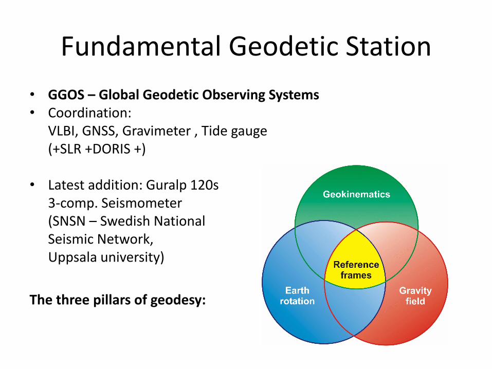
Fundamental Geodetic Station
• GGOS – Global Geodetic Observing Systems• Coordination:
VLBI, GNSS, Gravimeter , Tide gauge(+SLR +DORIS +)
• Latest addition: Guralp 120s3-comp. Seismometer(SNSN – Swedish NationalSeismic Network,Uppsala university)
The three pillars of geodesy: