4 Transmission System - Electrical...

Karady, George G. “Transmission System”The Electric Power Engineering HandbookEd. L.L. GrigsbyBoca Raton: CRC Press LLC, 2001

© 2001 CRC Press LLC

4Transmission SystemGeorge G. KaradyArizona State University

4.1 Concept of Energy Transmission and Distribution George G. Karady

4.2 Transmission Line Structures Joe C. Pohlman

4.3 Insulators and Accessories George G. Karady and R.G. Farmer

4.4 Transmission Line Construction and Maintenance Wilford Caulkins and Kristine Buchholz

4.5 Insulated Power Cables for High-Voltage Applications Carlos V. Núñez-Noriega and Felimón Hernandez

4.6 Transmission Line Parameters Manuel Reta-Hernández

4.7 Sag and Tension of Conductor D.A. Douglass and Ridley Thrash

4.8 Corona and Noise Giao N. Trinh

4.9 Geomagnetic Disturbances and Impacts upon Power System OperationJohn G. Kappenman

4.10 Lightning Protection William A. Chisholm

4.11 Reactive Power Compensation Rao S. Thallam


4Transmission System

4.1 Concept of Energy Transmission and DistributionGeneration Stations • Switchgear • Control Devices • Concept of Energy Transmission and Distribution

4.2 Transmission Line StructuresTraditional Line Design Practice • Current Deterministic Design Practice • Improved Design Approaches

4.3 Insulators and AccessoriesElectrical Stresses on External Insulation • Ceramic (Porcelain and Glass) Insulators • Nonceramic (Composite) Insulators • Insulator Failure Mechanism • Methods for Improving Insulator Performance

4.4 Transmission Line Construction and MaintenanceTools • Equipment • Procedures • Helicopters

4.5 Insulated Power Cables for High-Voltage ApplicationsTypical Cable Description • Overview of Electric Parameters of Underground Power Cables • Underground Layout and Construction • Testing, Troubleshooting, and Fault Location

4.6 Transmission Line ParametersEquivalent Circuit • Resistance • Current-Carrying Capacity (Ampacity) • Inductance and Inductive Reactance • Capacitance and Capacitive Reactance • Characteristics of Overhead Conductors

4.7 Sag and Tension of ConductorCatenary Cables • Approximate Sag-Tension Calculations • Numerical Sag-Tension Calculations • Ruling Span Concept • Line Design Sag-Tension Parameters • Conductor Installation

4.8 Corona and NoiseCorona Modes • Main Effects of Discharges on Overhead Lines • Impact on the Selection of Line Conductors • Conclusions

4.9 Geomagnetic Disturbances and Impacts upon Power System OperationPower System Reliability Threat • Transformer Impacts Due to GIC • Magneto-Telluric Climatology and the Dynamics of a Geomagnetic Superstorm • Satellite Monitoring and Forecast Models Advance Forecast Capabilities

4.10 Lightning ProtectionGround Flash Density • Stroke Incidence to Power Lines • Stroke Current Parameters • Calculation of Lightning Overvoltages on Shielded Lines • Insulation Strength • Conclusion

George G. KaradyArizona State University

Joe C. PohlmanConsultant

R.G. FarmerArizona State University

Wilford CaulkinsSherman & Reilly

Kristine BuchholzPacific Gas & Electric Company

Carlos V. Núñez-NoriegaGlendale Community College

Felimón HernandezArizona Public Service Company

Manuel Reta-HernándezArizona State University

D.A. DouglassPower Delivery Consultants, Inc.

Ridley ThrashSouthwire Company

Giao N. TrinhLog-In

John G. KappenmanMetatech Corporation

William A. ChisholmOntario Hydro Technologies

Rao S. ThallamSalt River Project


4.11 Reactive Power CompensationThe Need for Reactive Power Compensation • Application of Shunt Capacitor Banks in Distribution Systems — A Utility Perspective • Static VAR Control (SVC) • Series Compensation • Series Capacitor Bank

4.1 Concept of Energy Transmission and Distribution

George G. Karady

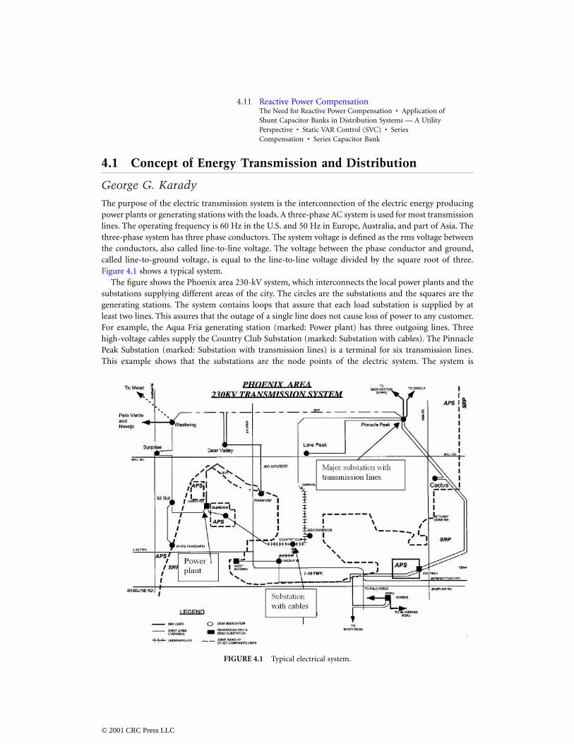
The purpose of the electric transmission system is the interconnection of the electric energy producingpower plants or generating stations with the loads. A three-phase AC system is used for most transmissionlines. The operating frequency is 60 Hz in the U.S. and 50 Hz in Europe, Australia, and part of Asia. Thethree-phase system has three phase conductors. The system voltage is defined as the rms voltage betweenthe conductors, also called line-to-line voltage. The voltage between the phase conductor and ground,called line-to-ground voltage, is equal to the line-to-line voltage divided by the square root of three.Figure 4.1 shows a typical system.

The figure shows the Phoenix area 230-kV system, which interconnects the local power plants and thesubstations supplying different areas of the city. The circles are the substations and the squares are thegenerating stations. The system contains loops that assure that each load substation is supplied by atleast two lines. This assures that the outage of a single line does not cause loss of power to any customer.For example, the Aqua Fria generating station (marked: Power plant) has three outgoing lines. Threehigh-voltage cables supply the Country Club Substation (marked: Substation with cables). The PinnaclePeak Substation (marked: Substation with transmission lines) is a terminal for six transmission lines.This example shows that the substations are the node points of the electric system. The system is

FIGURE 4.1 Typical electrical system.


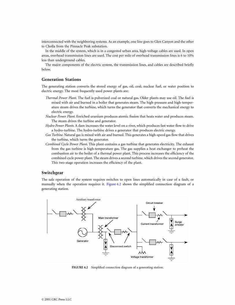
interconnected with the neighboring systems. As an example, one line goes to Glen Canyon and the otherto Cholla from the Pinnacle Peak substation.

In the middle of the system, which is in a congested urban area, high-voltage cables are used. In openareas, overhead transmission lines are used. The cost per mile of overhead transmission lines is 6 to 10%less than underground cables.

The major components of the electric system, the transmission lines, and cables are described brieflybelow.

Generation Stations

The generating station converts the stored energy of gas, oil, coal, nuclear fuel, or water position toelectric energy. The most frequently used power plants are:

Thermal Power Plant. The fuel is pulverized coal or natural gas. Older plants may use oil. The fuel ismixed with air and burned in a boiler that generates steam. The high-pressure and high-temper-ature steam drives the turbine, which turns the generator that converts the mechanical energy toelectric energy.

Nuclear Power Plant. Enriched uranium produces atomic fission that heats water and produces steam.The steam drives the turbine and generator.

Hydro Power Plants. A dam increases the water level on a river, which produces fast water flow to drivea hydro-turbine. The hydro-turbine drives a generator that produces electric energy.

Gas Turbine. Natural gas is mixed with air and burned. This generates a high-speed gas flow that drivesthe turbine, which turns the generator.

Combined Cycle Power Plant. This plant contains a gas turbine that generates electricity. The exhaustfrom the gas turbine is high-temperature gas. The gas supplies a heat exchanger to preheat thecombustion air to the boiler of a thermal power plant. This process increases the efficiency of thecombined cycle power plant. The steam drives a second turbine, which drives the second generator.This two-stage operation increases the efficiency of the plant.

Switchgear

The safe operation of the system requires switches to open lines automatically in case of a fault, ormanually when the operation requires it. Figure 4.2 shows the simplified connection diagram of agenerating station.

FIGURE 4.2 Simplified connection diagram of a generating station.


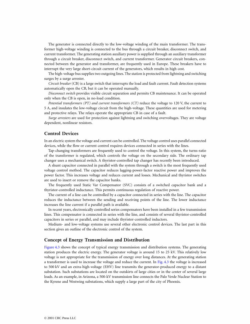
The generator is connected directly to the low-voltage winding of the main transformer. The trans-former high-voltage winding is connected to the bus through a circuit breaker, disconnect switch, andcurrent transformer. The generating station auxiliary power is supplied through an auxiliary transformerthrough a circuit breaker, disconnect switch, and current transformer. Generator circuit breakers, con-nected between the generator and transformer, are frequently used in Europe. These breakers have tointerrupt the very large short-circuit current of the generators, which results in high cost.

The high-voltage bus supplies two outgoing lines. The station is protected from lightning and switchingsurges by a surge arrester.

Circuit breaker (CB) is a large switch that interrupts the load and fault current. Fault detection systemsautomatically open the CB, but it can be operated manually.

Disconnect switch provides visible circuit separation and permits CB maintenance. It can be operatedonly when the CB is open, in no-load condition.

Potential transformers (PT) and current transformers (CT) reduce the voltage to 120 V, the current to5 A, and insulates the low-voltage circuit from the high-voltage. These quantities are used for meteringand protective relays. The relays operate the appropriate CB in case of a fault.

Surge arresters are used for protection against lightning and switching overvoltages. They are voltagedependent, nonlinear resistors.

Control Devices

In an electric system the voltage and current can be controlled. The voltage control uses parallel connecteddevices, while the flow or current control requires devices connected in series with the lines.

Tap-changing transformers are frequently used to control the voltage. In this system, the turns-ratioof the transformer is regulated, which controls the voltage on the secondary side. The ordinary tapchanger uses a mechanical switch. A thyristor-controlled tap changer has recently been introduced.

A shunt capacitor connected in parallel with the system through a switch is the most frequently usedvoltage control method. The capacitor reduces lagging-power-factor reactive power and improves thepower factor. This increases voltage and reduces current and losses. Mechanical and thyristor switchesare used to insert or remove the capacitor banks.

The frequently used Static Var Compensator (SVC) consists of a switched capacitor bank and athyristor-controlled inductance. This permits continuous regulation of reactive power.

The current of a line can be controlled by a capacitor connected in series with the line. The capacitorreduces the inductance between the sending and receiving points of the line. The lower inductanceincreases the line current if a parallel path is available.

In recent years, electronically controlled series compensators have been installed in a few transmissionlines. This compensator is connected in series with the line, and consists of several thyristor-controlledcapacitors in series or parallel, and may include thyristor-controlled inductors.

Medium- and low-voltage systems use several other electronic control devices. The last part in thissection gives an outline of the electronic control of the system.

Concept of Energy Transmission and Distribution

Figure 4.3 shows the concept of typical energy transmission and distribution systems. The generatingstation produces the electric energy. The generator voltage is around 15 to 25 kV. This relatively lowvoltage is not appropriate for the transmission of energy over long distances. At the generating stationa transformer is used to increase the voltage and reduce the current. In Fig. 4.3 the voltage is increasedto 500 kV and an extra-high-voltage (EHV) line transmits the generator-produced energy to a distantsubstation. Such substations are located on the outskirts of large cities or in the center of several largeloads. As an example, in Arizona, a 500-kV transmission line connects the Palo Verde Nuclear Station tothe Kyrene and Westwing substations, which supply a large part of the city of Phoenix.


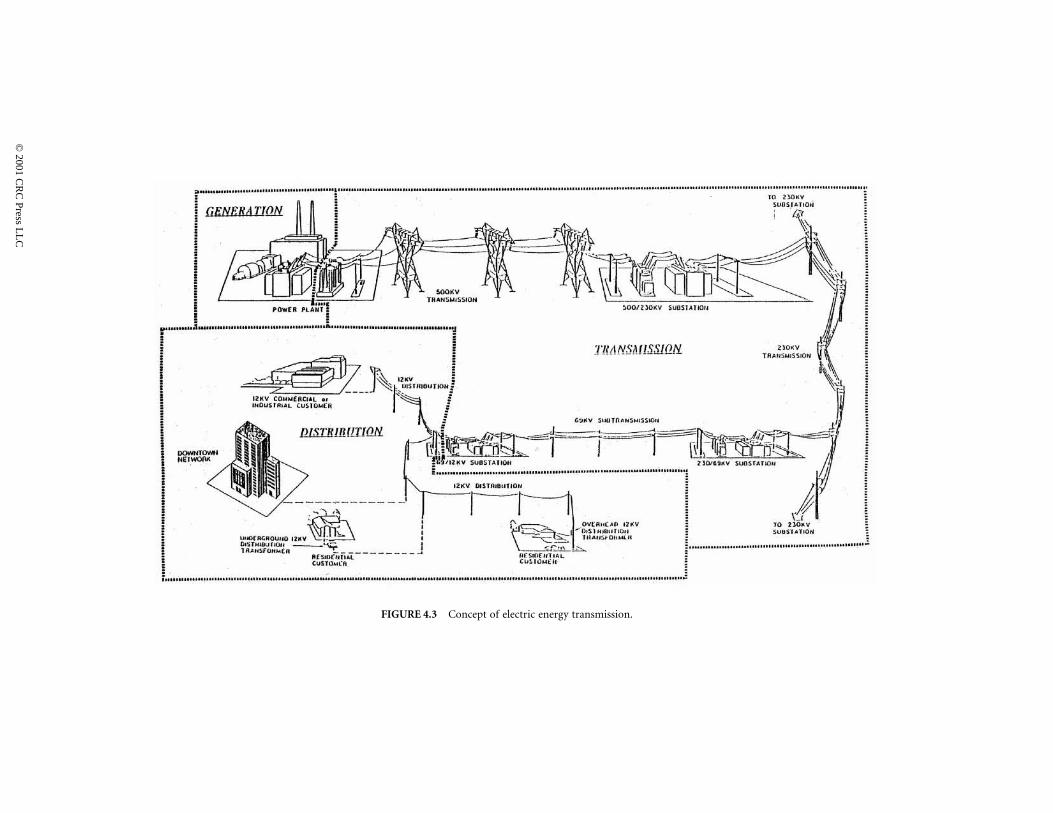
FIGURE 4.3 Concept of electric energy transmission.

©

2001 CR

C Press L

LC

The voltage is reduced at the 500 kV/220 kV EHV substation to the high-voltage level and high-voltagelines transmit the energy to high-voltage substations located within cities.

At the high-voltage substation the voltage is reduced to 69 kV. Sub-transmission lines connect thehigh-voltage substation to many local distribution stations located within cities. Sub-transmission linesare frequently located along major streets.

The voltage is reduced to 12 kV at the distribution substation. Several distribution lines emanate fromeach distribution substation as overhead or underground lines. Distribution lines distribute the energyalong streets and alleys. Each line supplies several step-down transformers distributed along the line. Thedistribution transformer reduces the voltage to 230/115 V, which supplies houses, shopping centers, andother local loads. The large industrial plants and factories are supplied directly by a subtransmission lineor a dedicated distribution line as shown in Fig. 4.3.

The overhead transmission lines are used in open areas such as interconnections between cities oralong wide roads within the city. In congested areas within cities, underground cables are used for electricenergy transmission. The underground transmission system is environmentally preferable but has asignificantly higher cost. In Fig. 4.3 the 12-kV line is connected to a 12-kV cable which supplies com-mercial or industrial customers. The figure also shows 12-kV cable networks supplying downtown areasin a large city. Most newly developed residential areas are supplied by 12-kV cables through pad-mountedstep-down transformers as shown in Fig. 4.3.

High-Voltage Transmission Lines

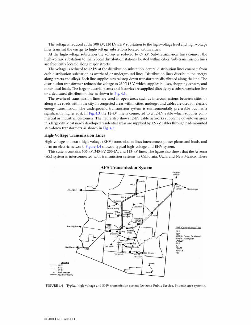
High-voltage and extra-high-voltage (EHV) transmission lines interconnect power plants and loads, andform an electric network. Figure 4.4 shows a typical high-voltage and EHV system.

This system contains 500-kV, 345-kV, 230-kV, and 115-kV lines. The figure also shows that the Arizona(AZ) system is interconnected with transmission systems in California, Utah, and New Mexico. These

FIGURE 4.4 Typical high-voltage and EHV transmission system (Arizona Public Service, Phoenix area system).


interconnections provide instantaneous help in case of lost generation in the AZ system. This also permitsthe export or import of energy, depending on the needs of the areas.

Presently, synchronous ties (AC lines) interconnect all networks in the eastern U.S. and Canada.Synchronous ties also (AC lines) interconnect all networks in the western U.S. and Canada. Several non-synchronous ties (DC lines) connect the East and the West. These interconnections increase the reliabilityof the electric supply systems.

In the U.S., the nominal voltage of the high-voltage lines is between 100 kV and 230 kV. The voltageof the extra-high-voltage lines is above 230 kV and below 800 kV. The voltage of an ultra-high-voltageline is above 800 kV. The maximum length of high-voltage lines is around 200 miles. Extra-high-voltagetransmission lines generally supply energy up to 400–500 miles without intermediate switching and varsupport. Transmission lines are terminated at the bus of a substation.

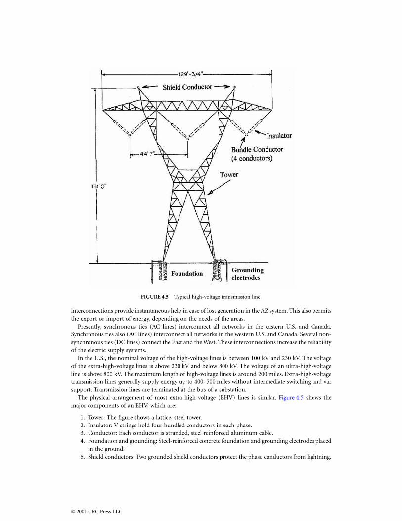
The physical arrangement of most extra-high-voltage (EHV) lines is similar. Figure 4.5 shows themajor components of an EHV, which are:

1. Tower: The figure shows a lattice, steel tower.2. Insulator: V strings hold four bundled conductors in each phase.3. Conductor: Each conductor is stranded, steel reinforced aluminum cable.4. Foundation and grounding: Steel-reinforced concrete foundation and grounding electrodes placed

in the ground.5. Shield conductors: Two grounded shield conductors protect the phase conductors from lightning.

FIGURE 4.5 Typical high-voltage transmission line.


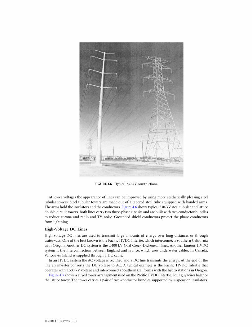
At lower voltages the appearance of lines can be improved by using more aesthetically pleasing steeltubular towers. Steel tubular towers are made out of a tapered steel tube equipped with banded arms.The arms hold the insulators and the conductors. Figure 4.6 shows typical 230-kV steel tubular and latticedouble-circuit towers. Both lines carry two three-phase circuits and are built with two conductor bundlesto reduce corona and radio and TV noise. Grounded shield conductors protect the phase conductorsfrom lightning.

High-Voltage DC Lines

High-voltage DC lines are used to transmit large amounts of energy over long distances or throughwaterways. One of the best known is the Pacific HVDC Intertie, which interconnects southern Californiawith Oregon. Another DC system is the ±400 kV Coal Creek-Dickenson lines. Another famous HVDCsystem is the interconnection between England and France, which uses underwater cables. In Canada,Vancouver Island is supplied through a DC cable.

In an HVDC system the AC voltage is rectified and a DC line transmits the energy. At the end of theline an inverter converts the DC voltage to AC. A typical example is the Pacific HVDC Intertie thatoperates with ±500 kV voltage and interconnects Southern California with the hydro stations in Oregon.

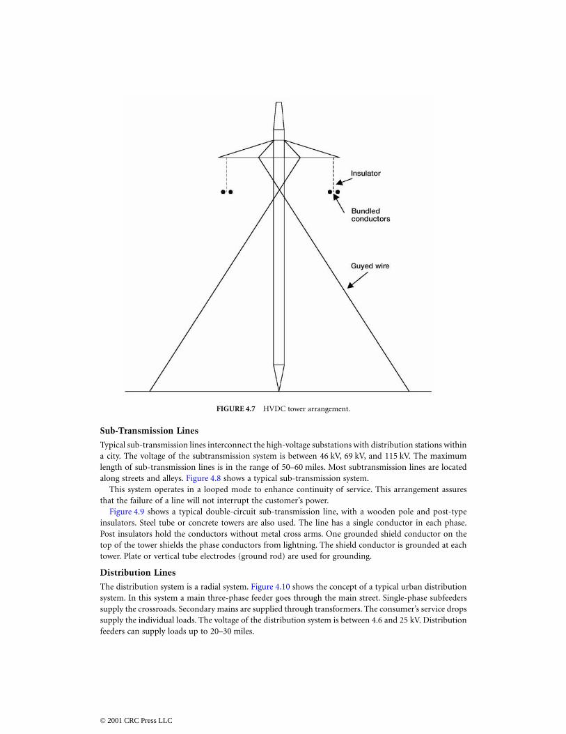
Figure 4.7 shows a guyed tower arrangement used on the Pacific HVDC Intertie. Four guy wires balancethe lattice tower. The tower carries a pair of two-conductor bundles supported by suspension insulators.

FIGURE 4.6 Typical 230-kV constructions.


Sub-Transmission Lines

Typical sub-transmission lines interconnect the high-voltage substations with distribution stations withina city. The voltage of the subtransmission system is between 46 kV, 69 kV, and 115 kV. The maximumlength of sub-transmission lines is in the range of 50–60 miles. Most subtransmission lines are locatedalong streets and alleys. Figure 4.8 shows a typical sub-transmission system.

This system operates in a looped mode to enhance continuity of service. This arrangement assuresthat the failure of a line will not interrupt the customer’s power.

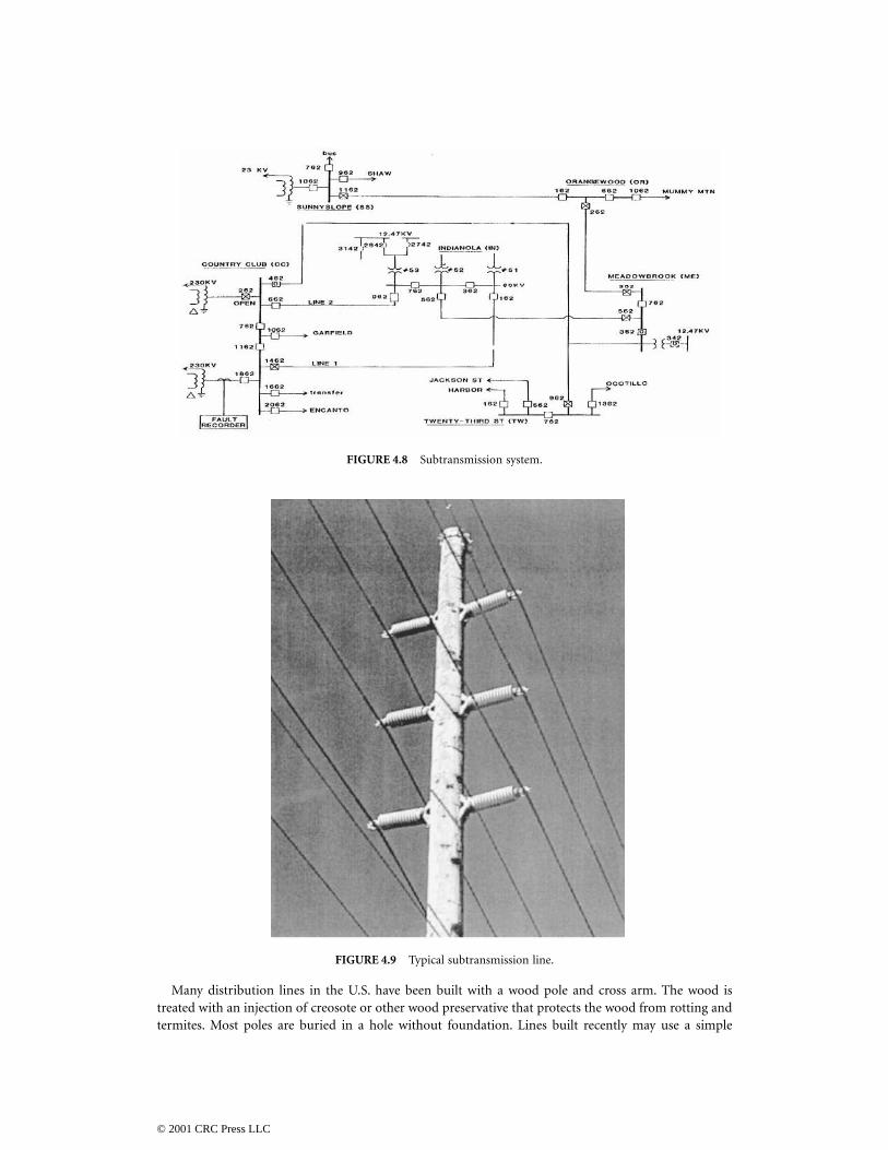
Figure 4.9 shows a typical double-circuit sub-transmission line, with a wooden pole and post-typeinsulators. Steel tube or concrete towers are also used. The line has a single conductor in each phase.Post insulators hold the conductors without metal cross arms. One grounded shield conductor on thetop of the tower shields the phase conductors from lightning. The shield conductor is grounded at eachtower. Plate or vertical tube electrodes (ground rod) are used for grounding.

Distribution Lines

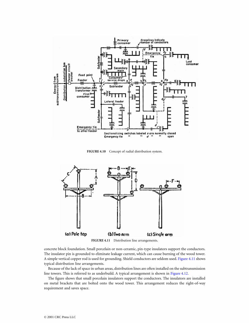
The distribution system is a radial system. Figure 4.10 shows the concept of a typical urban distributionsystem. In this system a main three-phase feeder goes through the main street. Single-phase subfeederssupply the crossroads. Secondary mains are supplied through transformers. The consumer’s service dropssupply the individual loads. The voltage of the distribution system is between 4.6 and 25 kV. Distributionfeeders can supply loads up to 20–30 miles.

FIGURE 4.7 HVDC tower arrangement.


Many distribution lines in the U.S. have been built with a wood pole and cross arm. The wood istreated with an injection of creosote or other wood preservative that protects the wood from rotting andtermites. Most poles are buried in a hole without foundation. Lines built recently may use a simple

FIGURE 4.8 Subtransmission system.

FIGURE 4.9 Typical subtransmission line.


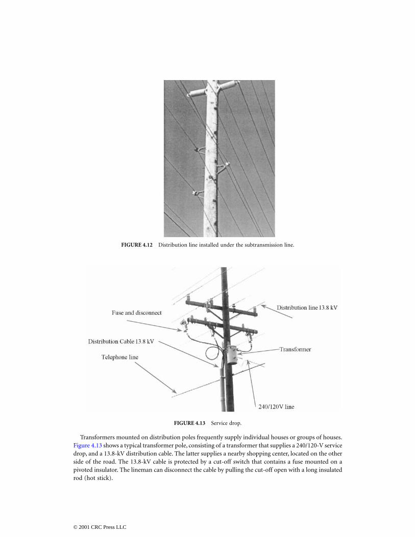
concrete block foundation. Small porcelain or non-ceramic, pin-type insulators support the conductors.The insulator pin is grounded to eliminate leakage current, which can cause burning of the wood tower.A simple vertical copper rod is used for grounding. Shield conductors are seldom used. Figure 4.11 showstypical distribution line arrangements.

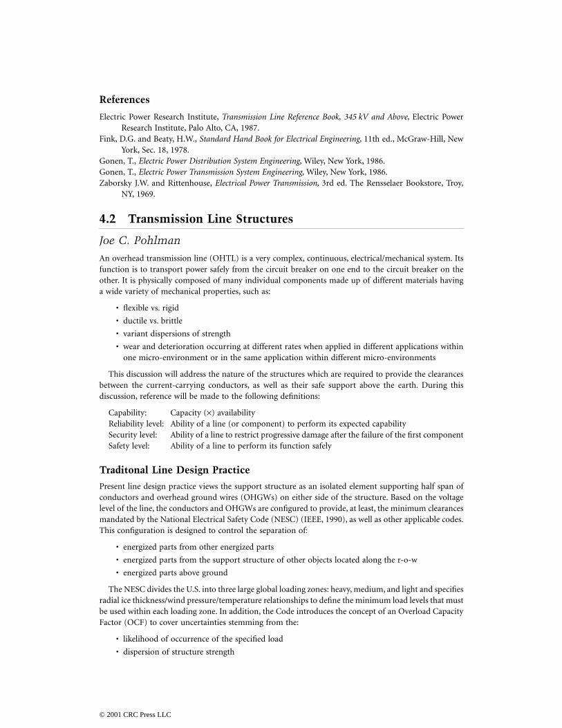
Because of the lack of space in urban areas, distribution lines are often installed on the subtransmissionline towers. This is referred to as underbuild. A typical arrangement is shown in Figure 4.12.

The figure shows that small porcelain insulators support the conductors. The insulators are installedon metal brackets that are bolted onto the wood tower. This arrangement reduces the right-of-wayrequirement and saves space.

FIGURE 4.10 Concept of radial distribution system.

FIGURE 4.11 Distribution line arrangements.


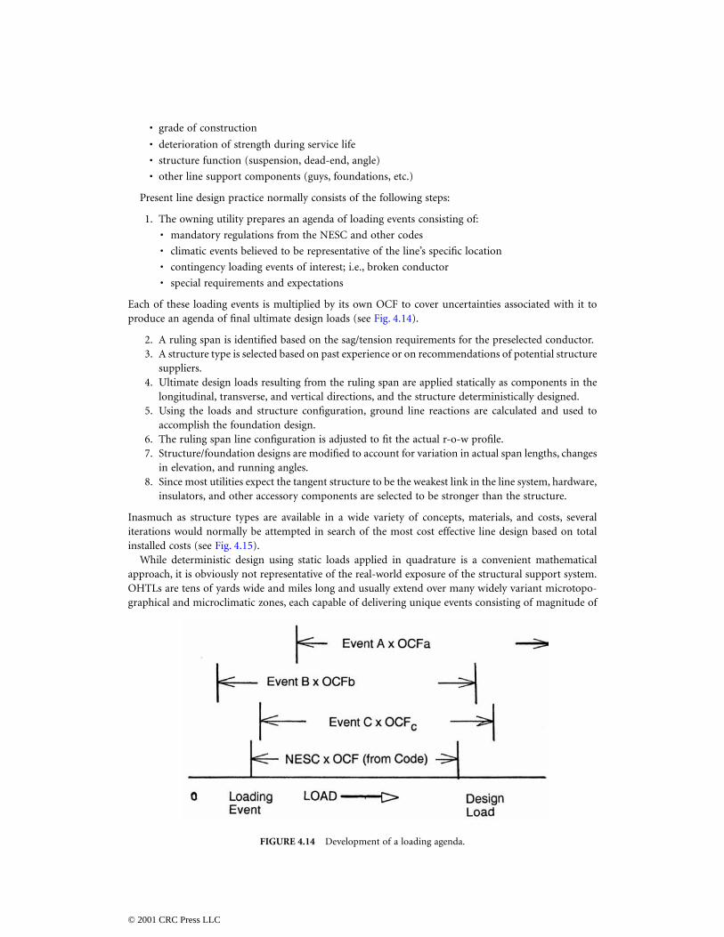
Transformers mounted on distribution poles frequently supply individual houses or groups of houses.Figure 4.13 shows a typical transformer pole, consisting of a transformer that supplies a 240/120-V servicedrop, and a 13.8-kV distribution cable. The latter supplies a nearby shopping center, located on the otherside of the road. The 13.8-kV cable is protected by a cut-off switch that contains a fuse mounted on apivoted insulator. The lineman can disconnect the cable by pulling the cut-off open with a long insulatedrod (hot stick).

FIGURE 4.12 Distribution line installed under the subtransmission line.

FIGURE 4.13 Service drop.


References

Electric Power Research Institute, Transmission Line Reference Book, 345 kV and Above, Electric PowerResearch Institute, Palo Alto, CA, 1987.

Fink, D.G. and Beaty, H.W., Standard Hand Book for Electrical Engineering, 11th ed., McGraw-Hill, NewYork, Sec. 18, 1978.

Gonen, T., Electric Power Distribution System Engineering, Wiley, New York, 1986.Gonen, T., Electric Power Transmission System Engineering, Wiley, New York, 1986.Zaborsky J.W. and Rittenhouse, Electrical Power Transmission, 3rd ed. The Rensselaer Bookstore, Troy,

NY, 1969.

4.2 Transmission Line Structures

Joe C. Pohlman

An overhead transmission line (OHTL) is a very complex, continuous, electrical/mechanical system. Itsfunction is to transport power safely from the circuit breaker on one end to the circuit breaker on theother. It is physically composed of many individual components made up of different materials havinga wide variety of mechanical properties, such as:

• flexible vs. rigid

• ductile vs. brittle

• variant dispersions of strength

• wear and deterioration occurring at different rates when applied in different applications withinone micro-environment or in the same application within different micro-environments

This discussion will address the nature of the structures which are required to provide the clearancesbetween the current-carrying conductors, as well as their safe support above the earth. During thisdiscussion, reference will be made to the following definitions:

Capability: Capacity (×) availabilityReliability level: Ability of a line (or component) to perform its expected capabilitySecurity level: Ability of a line to restrict progressive damage after the failure of the first componentSafety level: Ability of a line to perform its function safely

Traditonal Line Design Practice

Present line design practice views the support structure as an isolated element supporting half span ofconductors and overhead ground wires (OHGWs) on either side of the structure. Based on the voltagelevel of the line, the conductors and OHGWs are configured to provide, at least, the minimum clearancesmandated by the National Electrical Safety Code (NESC) (IEEE, 1990), as well as other applicable codes.This configuration is designed to control the separation of:

• energized parts from other energized parts

• energized parts from the support structure of other objects located along the r-o-w

• energized parts above ground

The NESC divides the U.S. into three large global loading zones: heavy, medium, and light and specifiesradial ice thickness/wind pressure/temperature relationships to define the minimum load levels that mustbe used within each loading zone. In addition, the Code introduces the concept of an Overload CapacityFactor (OCF) to cover uncertainties stemming from the:

• likelihood of occurrence of the specified load

• dispersion of structure strength


• grade of construction

• deterioration of strength during service life

• structure function (suspension, dead-end, angle)

• other line support components (guys, foundations, etc.)

Present line design practice normally consists of the following steps:

1. The owning utility prepares an agenda of loading events consisting of:

• mandatory regulations from the NESC and other codes

• climatic events believed to be representative of the line’s specific location

• contingency loading events of interest; i.e., broken conductor

• special requirements and expectations

Each of these loading events is multiplied by its own OCF to cover uncertainties associated with it toproduce an agenda of final ultimate design loads (see Fig. 4.14).

2. A ruling span is identified based on the sag/tension requirements for the preselected conductor.3. A structure type is selected based on past experience or on recommendations of potential structure

suppliers.4. Ultimate design loads resulting from the ruling span are applied statically as components in the

longitudinal, transverse, and vertical directions, and the structure deterministically designed.5. Using the loads and structure configuration, ground line reactions are calculated and used to

accomplish the foundation design.6. The ruling span line configuration is adjusted to fit the actual r-o-w profile.7. Structure/foundation designs are modified to account for variation in actual span lengths, changes

in elevation, and running angles.8. Since most utilities expect the tangent structure to be the weakest link in the line system, hardware,

insulators, and other accessory components are selected to be stronger than the structure.

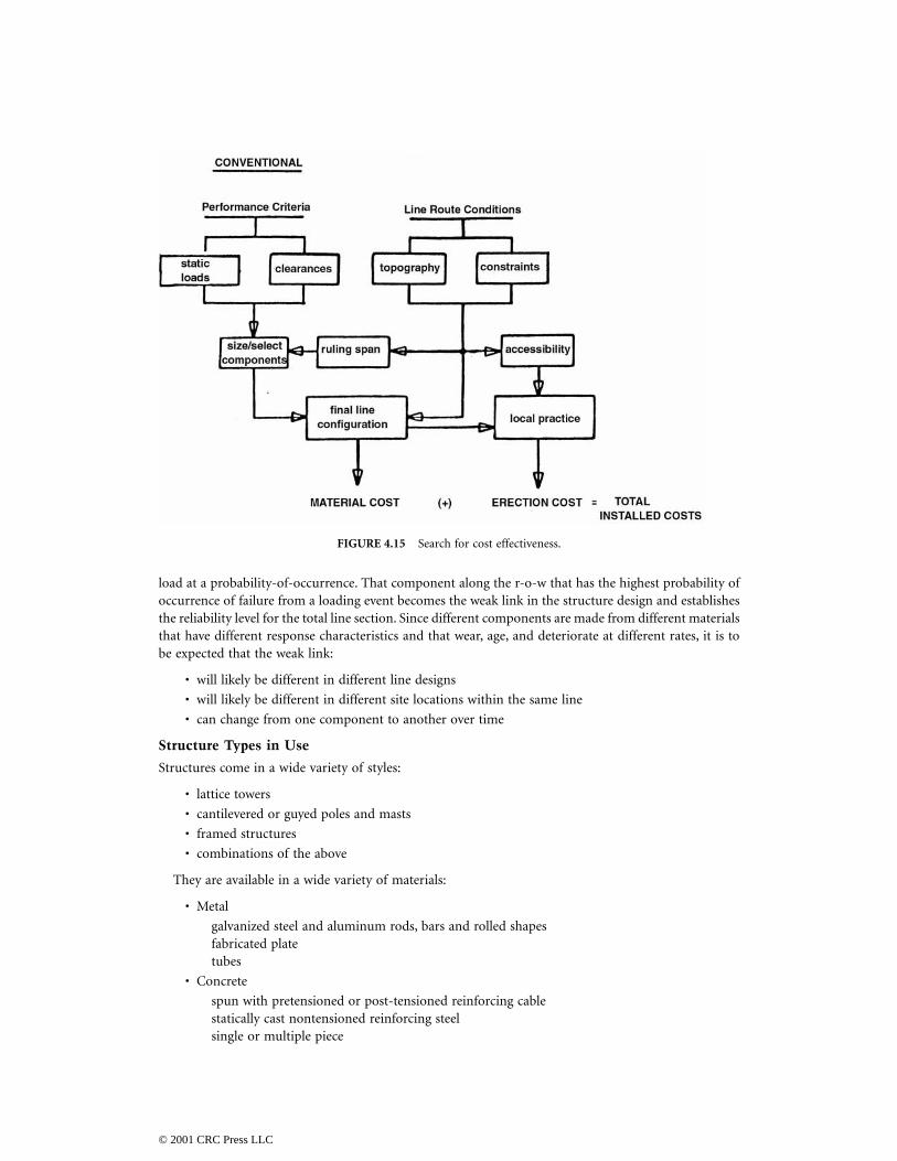
Inasmuch as structure types are available in a wide variety of concepts, materials, and costs, severaliterations would normally be attempted in search of the most cost effective line design based on totalinstalled costs (see Fig. 4.15).

While deterministic design using static loads applied in quadrature is a convenient mathematicalapproach, it is obviously not representative of the real-world exposure of the structural support system.OHTLs are tens of yards wide and miles long and usually extend over many widely variant microtopo-graphical and microclimatic zones, each capable of delivering unique events consisting of magnitude of

FIGURE 4.14 Development of a loading agenda.


load at a probability-of-occurrence. That component along the r-o-w that has the highest probability ofoccurrence of failure from a loading event becomes the weak link in the structure design and establishesthe reliability level for the total line section. Since different components are made from different materialsthat have different response characteristics and that wear, age, and deteriorate at different rates, it is tobe expected that the weak link:

• will likely be different in different line designs

• will likely be different in different site locations within the same line

• can change from one component to another over time

Structure Types in Use

Structures come in a wide variety of styles:

• lattice towers

• cantilevered or guyed poles and masts

• framed structures

• combinations of the above

They are available in a wide variety of materials:

• Metal

galvanized steel and aluminum rods, bars and rolled shapesfabricated platetubes

• Concrete

spun with pretensioned or post-tensioned reinforcing cablestatically cast nontensioned reinforcing steelsingle or multiple piece

FIGURE 4.15 Search for cost effectiveness.


• Wood

as grown

glued laminar

• Plastics

• Composites

• Crossarms and braces

• Variations of all of the above

Depending on their style and material contents, structures vary considerably in how they respond toload. Some are rigid. Some are flexible. Those structures that can safely deflect under load and absorbenergy while doing so, provide an ameliorating influence on progressive damage after the failure of thefirst element (Pohlman and Lummis, 1969).

Factors Affecting Structure Type Selection

There are usually many factors that impact on the selection of the structure type for use in an OHTL.Some of the more significant are briefly identified below.

Erection Technique: It is obvious that different structure types require different erection techniques. Asan example, steel lattice towers consist of hundreds of individual members that must be bolted together,assembled, and erected onto the four previously installed foundations. A tapered steel pole, on the otherhand, is likely to be produced in a single piece and erected directly on its previously installed foundationin one hoist. The lattice tower requires a large amount of labor to accomplish the considerable numberof bolted joints, whereas the pole requires the installation of a few nuts applied to the foundation anchorbolts plus a few to install the crossarms. The steel pole requires a large-capacity crane with a high reachwhich would probably not be needed for the tower. Therefore, labor needs to be balanced against theneed for large, special equipment and the site’s accessibility for such equipment.

Public Concerns: Probably the most difficult factors to deal with arise as a result of the concerns of thegeneral public living, working, or coming in proximity to the line. It is common practice to hold publichearings as part of the approval process for a new line. Such public hearings offer a platform for neighborsto express individual concerns that generally must be satisfactorily addressed before the required permitwill be issued. A few comments demonstrate this problem.

The general public usually perceives transmission structures as “eyesores” and distractions in the locallandscape. To combat this, an industry study was made in the late 1960s (Dreyfuss, 1968) sponsored bythe Edison Electric Institute and accomplished by Henry Dreyfuss, the internationally recognized indus-trial designer. While the guidelines did not overcome all the objections, they did provide a means ofsatisfying certain very highly controversial installations (Pohlman and Harris, 1971).

Parents of small children and safety engineers often raise the issue of lattice masts, towers, and guys,constituting an “attractive challenge” to determined climbers, particularly youngsters.

Inspection, Assessment, and Maintenance: Depending on the owning utility, it is likely their in-housepractices will influence the selection of the structure type for use in a specific line location. Inspectionsand assessment are usually made by human inspectors who use diagnostic technologies to augment theirpersonal senses of sight and touch. The nature and location of the symptoms of critical interest are suchthat they can be most effectively examined from specific perspectives. Inspectors must work from themost advantageous location when making inspections. Methods can include observations from groundor fly-by patrol, climbing, bucket trucks, or helicopters. Likewise, there are certain maintenance activitiesthat are known or believed to be required for particular structure types. The equipment necessary tomaintain the structure should be taken into consideration during the structure type selection process toassure there will be no unexpected conflict between maintenance needs and r-o-w restrictions.

Future Upgrading or Uprating: Because of the difficulty of procuring r-o-w’s and obtaining the necessarypermits to build new lines, many utilities improve their future options by selecting structure types forcurrent line projects that will permit future upgrading and/or uprating initiatives.


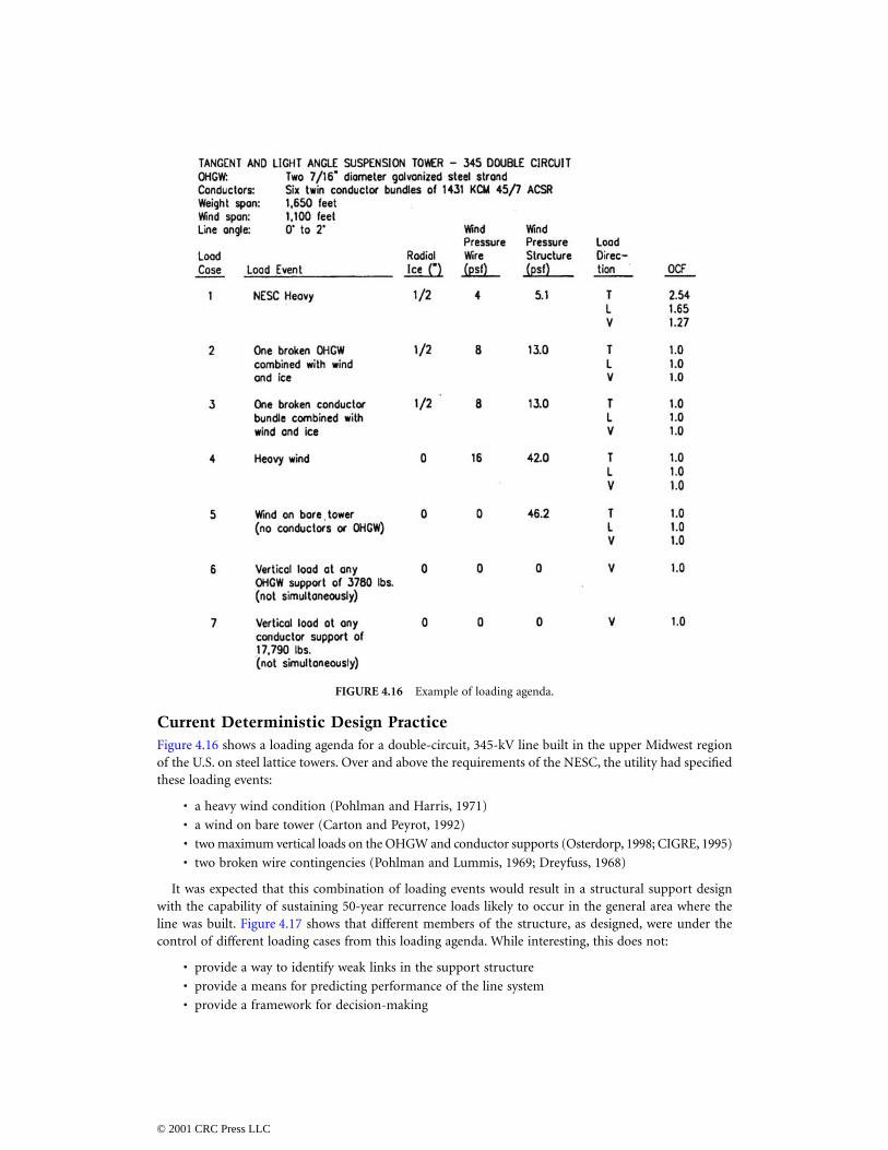
Current Deterministic Design PracticeFigure 4.16 shows a loading agenda for a double-circuit, 345-kV line built in the upper Midwest regionof the U.S. on steel lattice towers. Over and above the requirements of the NESC, the utility had specifiedthese loading events:

• a heavy wind condition (Pohlman and Harris, 1971)

• a wind on bare tower (Carton and Peyrot, 1992)

• two maximum vertical loads on the OHGW and conductor supports (Osterdorp, 1998; CIGRE, 1995)

• two broken wire contingencies (Pohlman and Lummis, 1969; Dreyfuss, 1968)

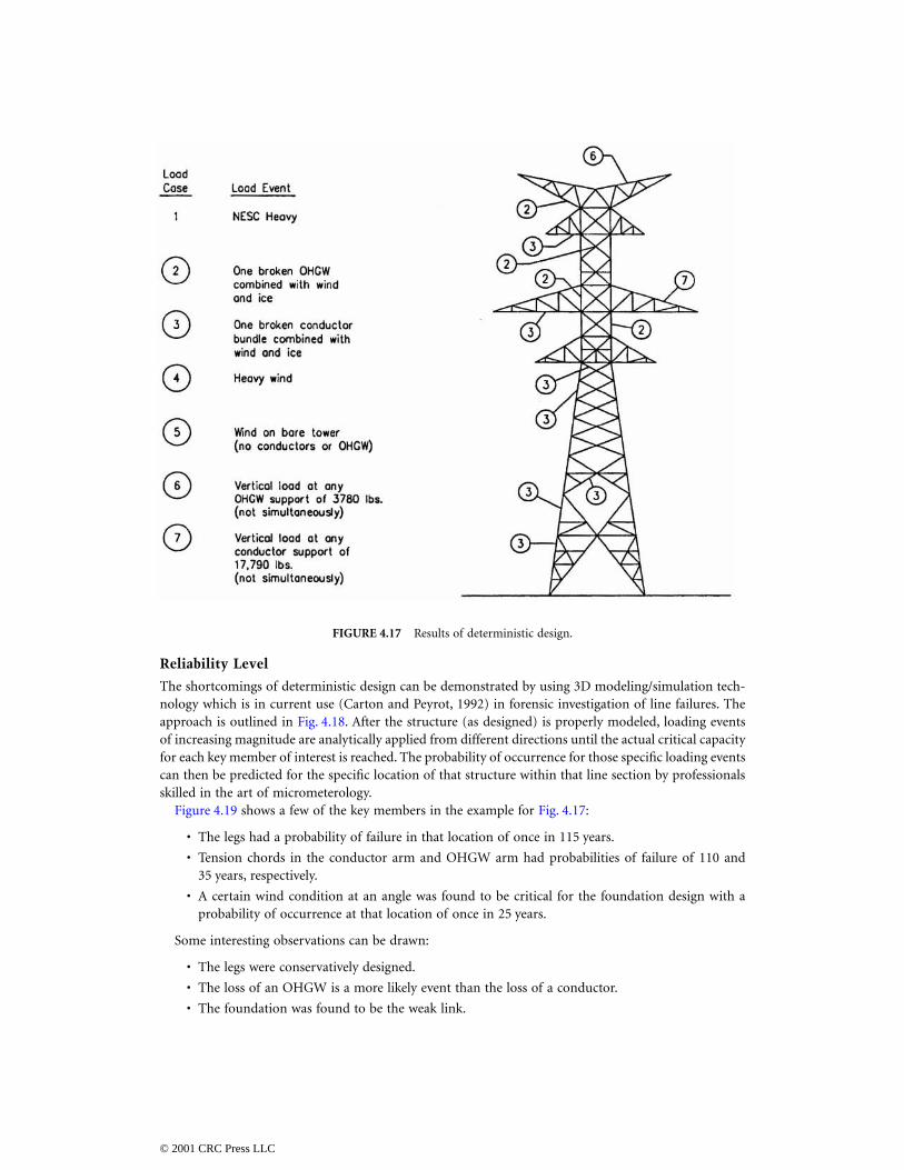
It was expected that this combination of loading events would result in a structural support designwith the capability of sustaining 50-year recurrence loads likely to occur in the general area where theline was built. Figure 4.17 shows that different members of the structure, as designed, were under thecontrol of different loading cases from this loading agenda. While interesting, this does not:

• provide a way to identify weak links in the support structure

• provide a means for predicting performance of the line system

• provide a framework for decision-making

FIGURE 4.16 Example of loading agenda.


Reliability Level

The shortcomings of deterministic design can be demonstrated by using 3D modeling/simulation tech-nology which is in current use (Carton and Peyrot, 1992) in forensic investigation of line failures. Theapproach is outlined in Fig. 4.18. After the structure (as designed) is properly modeled, loading eventsof increasing magnitude are analytically applied from different directions until the actual critical capacityfor each key member of interest is reached. The probability of occurrence for those specific loading eventscan then be predicted for the specific location of that structure within that line section by professionalsskilled in the art of micrometerology.

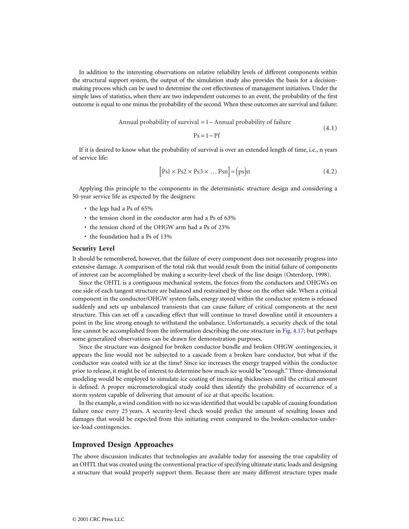
Figure 4.19 shows a few of the key members in the example for Fig. 4.17:

• The legs had a probability of failure in that location of once in 115 years.

• Tension chords in the conductor arm and OHGW arm had probabilities of failure of 110 and35 years, respectively.

• A certain wind condition at an angle was found to be critical for the foundation design with aprobability of occurrence at that location of once in 25 years.

Some interesting observations can be drawn:

• The legs were conservatively designed.

• The loss of an OHGW is a more likely event than the loss of a conductor.

• The foundation was found to be the weak link.

FIGURE 4.17 Results of deterministic design.


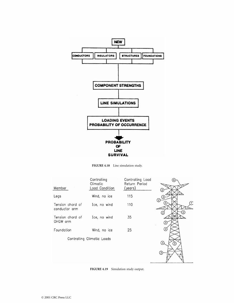
FIGURE 4.18 Line simulation study.

FIGURE 4.19 Simulation study output.


In addition to the interesting observations on relative reliability levels of different components withinthe structural support system, the output of the simulation study also provides the basis for a decision-making process which can be used to determine the cost effectiveness of management initiatives. Under thesimple laws of statistics, when there are two independent outcomes to an event, the probability of the firstoutcome is equal to one minus the probability of the second. When these outcomes are survival and failure:

(4.1)

If it is desired to know what the probability of survival is over an extended length of time, i.e., n yearsof service life:

(4.2)

Applying this principle to the components in the deterministic structure design and considering a50-year service life as expected by the designers:

• the legs had a Ps of 65%

• the tension chord in the conductor arm had a Ps of 63%

• the tension chord of the OHGW arm had a Ps of 23%

• the foundation had a Ps of 13%

Security Level

It should be remembered, however, that the failure of every component does not necessarily progress intoextensive damage. A comparison of the total risk that would result from the initial failure of componentsof interest can be accomplished by making a security-level check of the line design (Osterdorp, 1998).

Since the OHTL is a contiguous mechanical system, the forces from the conductors and OHGWs onone side of each tangent structure are balanced and restrained by those on the other side. When a criticalcomponent in the conductor/OHGW system fails, energy stored within the conductor system is releasedsuddenly and sets up unbalanced transients that can cause failure of critical components at the nextstructure. This can set off a cascading effect that will continue to travel downline until it encounters apoint in the line strong enough to withstand the unbalance. Unfortunately, a security check of the totalline cannot be accomplished from the information describing the one structure in Fig. 4.17; but perhapssome generalized observations can be drawn for demonstration purposes.

Since the structure was designed for broken conductor bundle and broken OHGW contingencies, itappears the line would not be subjected to a cascade from a broken bare conductor, but what if theconductor was coated with ice at the time? Since ice increases the energy trapped within the conductorprior to release, it might be of interest to determine how much ice would be “enough.” Three-dimensionalmodeling would be employed to simulate ice coating of increasing thicknesses until the critical amountis defined. A proper micrometerological study could then identify the probability of occurrence of astorm system capable of delivering that amount of ice at that specific location.

In the example, a wind condition with no ice was identified that would be capable of causing foundationfailure once every 25 years. A security-level check would predict the amount of resulting losses anddamages that would be expected from this initiating event compared to the broken-conductor-under-ice-load contingencies.

Improved Design Approaches

The above discussion indicates that technologies are available today for assessing the true capability ofan OHTL that was created using the conventional practice of specifying ultimate static loads and designinga structure that would properly support them. Because there are many different structure types made

Annual probability of survival nnual probability of failure= −

= −

1

1

A

Ps Pf

Ps Ps Ps Psn ps n1 2 3× × × …[ ] = ( )


from different materials, this was not always straightforward. Accordingly, many technical societiesprepared guidelines on how to design the specific structure needed. These are listed in the accompanyingreferences. The interested reader should realize that these documents are subject to periodic review andrevision and should, therefore, seek the most current version.

While the technical fraternity recognizes that the mentioned technologies are useful for analyzing existinglines and determining management initiatives, something more direct for designing new lines is needed.There are many efforts under way. The most promising of these is Improved Design Criteria of OHTLs Basedon Reliability Concepts (Ostendorp, 1998), currently under development by CIGRE Study Committee 22:Recommendations for Overhead Lines. Appendix A outlines the methodology involved in words and in adiagram. The technique is based on the premise that loads and strengths are stochastic variables and thecombined reliability is computable if the statistical functions of loads and strength are known. The referencedreport has been circulated internationally for trial use and comment. It is expected that the returnedcomments will be carefully considered, integrated into the report, and the final version submitted to theInternational Electrotechnical Commission (IEC) for consideration as an International Standard.

References

1. Carton, T. and Peyrot, A., Computer Aided Structural and Geometric Design of Power Lines, IEEETrans. on Power Line Syst., 7(1), 1992.

2. Dreyfuss, H., Electric Transmission Structures, Edison Electric Institute Publication No. 67-61, 1968.3. Guide for the Design and Use of Concrete Poles, ASCE 596-6, 1987.4. Guide for the Design of Prestressed Concrete Poles, ASCE/PCI Joint Commission on Concrete

Poles, February, 1992. Draft.5. Guide for the Design of Transmission Towers, ASCE Manual on Engineering Practice, 52, 1988.6. Guide for the Design Steel Transmission Poles, ASCE Manual on Engineering Practice, 72, 1990.7. IEEE Trial-Use Design Guide for Wood Transmission Structures, IEEE Std. 751, February, 1991.8. Improved Design Criteria of Overhead Transmission Lines Based on Reliability Concepts, CIGRE

SC-22 Report, October 1995.9. National Electrical Safety Code ANSI C-2, IEEE, 1990.

10. Ostendorp, M., Longitudinal Loading and Cascading Failure Assessment for Transmission LineUpgrades, ESMO Conference ’98, Orlando, Florida, April 26-30, 1998.

11. Pohlman, J. and Harris, W., Tapered Steel H-Frames Gain Acceptance Through Scenic Valley,Electric Light and Power Magazine, 48(vii), 55-58, 1971.

12. Pohlman, J. and Lummis, J., Flexible Structures Offer Broken Wire Integrity at Low Cost, ElectricLight and Power, 46(V, 144-148.4), 1969.

Appendix A — General Design Criteria — Methodology

The recommended methodology for designing transmission line components is summarized in Fig. 4.20and can be described as follows:

a) Gather preliminary line design data and available climatic data.1

b1) Select the reliability level in terms of return period of design loads. (Note: Some national regu-lations and/or codes of practice sometimes impose design requirements, directly or indirectly, thatmay restrict the choice offered to designers).

b2) Select the security requirements (failure containment).b3) List safety requirements imposed by mandatory regulations and construction and maintenance

loads.c) Calculate climatic variables corresponding to selected return period of design loads.

1In some countries, design wind speed, such as the 50-year return period, is given in National Standards.


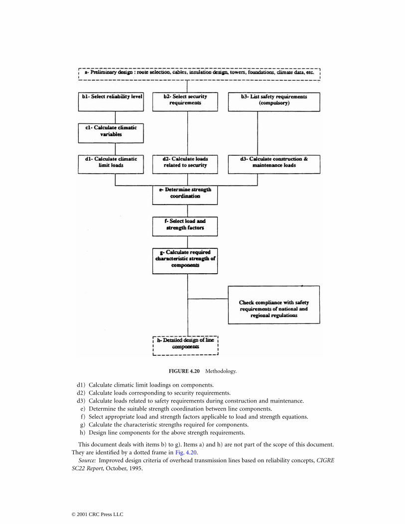
d1) Calculate climatic limit loadings on components.d2) Calculate loads corresponding to security requirements.d3) Calculate loads related to safety requirements during construction and maintenance.

e) Determine the suitable strength coordination between line components.f) Select appropriate load and strength factors applicable to load and strength equations.g) Calculate the characteristic strengths required for components.h) Design line components for the above strength requirements.

This document deals with items b) to g). Items a) and h) are not part of the scope of this document.They are identified by a dotted frame in Fig. 4.20.

Source: Improved design criteria of overhead transmission lines based on reliability concepts, CIGRESC22 Report, October, 1995.

FIGURE 4.20 Methodology.


4.3 Insulators and Accessories

George G. Karady and R.G. Farmer

Electric insulation is a vital part of an electrical power system. Although the cost of insulation is only asmall fraction of the apparatus or line cost, line performance is highly dependent on insulation integrity.Insulation failure may cause permanent equipment damage and long-term outages. As an example, ashort circuit in a 500-kV system may result in a loss of power to a large area for several hours. Thepotential financial losses emphasize the importance of a reliable design of the insulation.

The insulation of an electric system is divided into two broad categories:

1. Internal insulation2. External insulation

Apparatus or equipment has mostly internal insulation. The insulation is enclosed in a groundedhousing which protects it from the environment. External insulation is exposed to the environment. Atypical example of internal insulation is the insulation for a large transformer where insulation betweenturns and between coils consists of solid (paper) and liquid (oil) insulation protected by a steel tank. Anovervoltage can produce internal insulation breakdown and a permanent fault.

External insulation is exposed to the environment. Typical external insulation is the porcelain insulatorssupporting transmission line conductors. An overvoltage caused by flashover produces only a temporaryfault. The insulation is self-restoring.

This section discusses external insulation used for transmission lines and substations.

Electrical Stresses on External Insulation

The external insulation (transmission line or substation) is exposed to electrical, mechanical, and envi-ronmental stresses. The applied voltage of an operating power system produces electrical stresses. Theweather and the surroundings (industry, rural dust, oceans, etc.) produce additional environmentalstresses. The conductor weight, wind, and ice can generate mechanical stresses. The insulators mustwithstand these stresses for long periods of time. It is anticipated that a line or substation will operatefor more than 20–30 years without changing the insulators. However, regular maintenance is needed tominimize the number of faults per year. A typical number of insulation failure-caused faults is 0.5–10 peryear, per 100 mi of line.

Transmission Lines and Substations

Transmission line and substation insulation integrity is one of the most dominant factors in power systemreliability. We will describe typical transmission lines and substations to demonstrate the basic conceptof external insulation application.

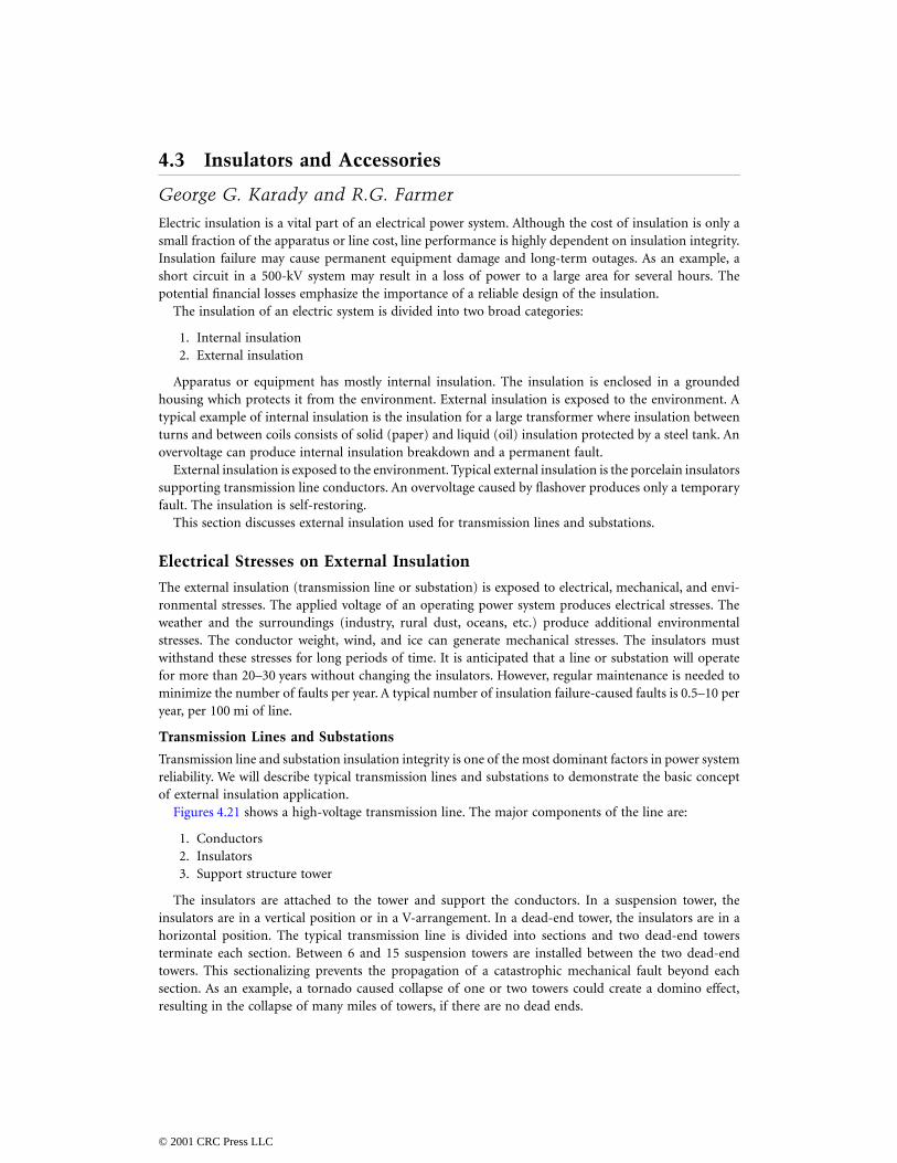
Figures 4.21 shows a high-voltage transmission line. The major components of the line are:

1. Conductors2. Insulators3. Support structure tower

The insulators are attached to the tower and support the conductors. In a suspension tower, theinsulators are in a vertical position or in a V-arrangement. In a dead-end tower, the insulators are in ahorizontal position. The typical transmission line is divided into sections and two dead-end towersterminate each section. Between 6 and 15 suspension towers are installed between the two dead-endtowers. This sectionalizing prevents the propagation of a catastrophic mechanical fault beyond eachsection. As an example, a tornado caused collapse of one or two towers could create a domino effect,resulting in the collapse of many miles of towers, if there are no dead ends.


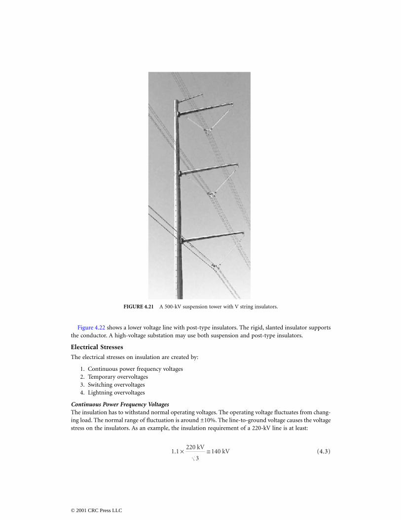
Figure 4.22 shows a lower voltage line with post-type insulators. The rigid, slanted insulator supportsthe conductor. A high-voltage substation may use both suspension and post-type insulators.

Electrical Stresses

The electrical stresses on insulation are created by:

1. Continuous power frequency voltages2. Temporary overvoltages3. Switching overvoltages4. Lightning overvoltages

Continuous Power Frequency VoltagesThe insulation has to withstand normal operating voltages. The operating voltage fluctuates from chang-ing load. The normal range of fluctuation is around ±10%. The line-to-ground voltage causes the voltagestress on the insulators. As an example, the insulation requirement of a 220-kV line is at least:

(4.3)

FIGURE 4.21 A 500-kV suspension tower with V string insulators.

1 1220

3140. × ≅kV

kV


This voltage is used for the selection of the number of insulators when the line is designed. Theinsulation can be laboratory tested by measuring the dry flashover voltage of the insulators. Because theline insulators are self-restoring, flashover tests do not cause any damage. The flashover voltage must belarger than the operating voltage to avoid outages. For a porcelain insulator, the required dry flashovervoltage is about 2.5–3 times the rated voltage. A significant number of the apparatus standards recom-mend dry withstand testing of every kind of insulation to be two (2) times the rated voltage plus 1 kVfor 1 min of time. This severe test eliminates most of the deficient units.

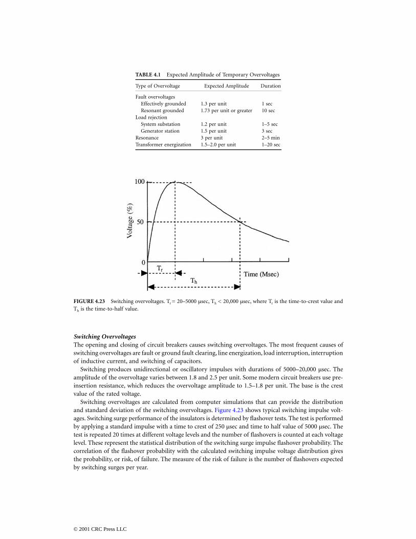
Temporary OvervoltagesThese include ground faults, switching, load rejection, line energization and resonance, cause powerfrequency, or close-to-power frequency, and relatively long duration overvoltages. The duration is from5 sec to several minutes. The expected peak amplitudes and duration are listed in Table 4.1.

The base is the crest value of the rated voltage. The dry withstand test, with two times the maximumoperating voltage plus 1 kV for 1 minute, is well-suited to test the performance of insulation undertemporary overvoltages.

FIGURE 4.22 69-kV transmission line with post insulators.


Switching OvervoltagesThe opening and closing of circuit breakers causes switching overvoltages. The most frequent causes ofswitching overvoltages are fault or ground fault clearing, line energization, load interruption, interruptionof inductive current, and switching of capacitors.

Switching produces unidirectional or oscillatory impulses with durations of 5000–20,000 µsec. Theamplitude of the overvoltage varies between 1.8 and 2.5 per unit. Some modern circuit breakers use pre-insertion resistance, which reduces the overvoltage amplitude to 1.5–1.8 per unit. The base is the crestvalue of the rated voltage.

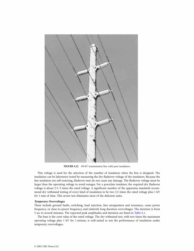
Switching overvoltages are calculated from computer simulations that can provide the distributionand standard deviation of the switching overvoltages. Figure 4.23 shows typical switching impulse volt-ages. Switching surge performance of the insulators is determined by flashover tests. The test is performedby applying a standard impulse with a time to crest of 250 µsec and time to half value of 5000 µsec. Thetest is repeated 20 times at different voltage levels and the number of flashovers is counted at each voltagelevel. These represent the statistical distribution of the switching surge impulse flashover probability. Thecorrelation of the flashover probability with the calculated switching impulse voltage distribution givesthe probability, or risk, of failure. The measure of the risk of failure is the number of flashovers expectedby switching surges per year.

TABLE 4.1 Expected Amplitude of Temporary Overvoltages

Type of Overvoltage Expected Amplitude Duration

Fault overvoltagesEffectively grounded 1.3 per unit 1 secResonant grounded 1.73 per unit or greater 10 sec

Load rejectionSystem substation 1.2 per unit 1–5 secGenerator station 1.5 per unit 3 sec

Resonance 3 per unit 2–5 minTransformer energization 1.5–2.0 per unit 1–20 sec

FIGURE 4.23 Switching overvoltages. Tr = 20–5000 µsec, Th < 20,000 µsec, where Tr is the time-to-crest value andTh is the time-to-half value.


Lightning OvervoltagesLightning overvoltages are caused by lightning strikes:

1. to the phase conductors2. to the shield conductor (the large current-caused voltage drop in the grounding resistance may

cause flashover to the conductors [back flash]).3. to the ground close to the line (the large ground current induces voltages in the phase conductors).

Lighting strikes cause a fast-rising, short-duration, unidirectional voltage pulse. The time-to-crest isbetween 0.1–20 µsec. The time-to-half value is 20–200 µsec.

The peak amplitude of the overvoltage generated by a direct strike to the conductor is very high and ispractically limited by the subsequent flashover of the insulation. Shielding failures and induced voltages causesomewhat less overvoltage. Shielding failure caused overvoltage is around 500 kV–2000 kV. The lightning-induced voltage is generally less than 400 kV. The actual stress on the insulators is equal to the impulse voltage.

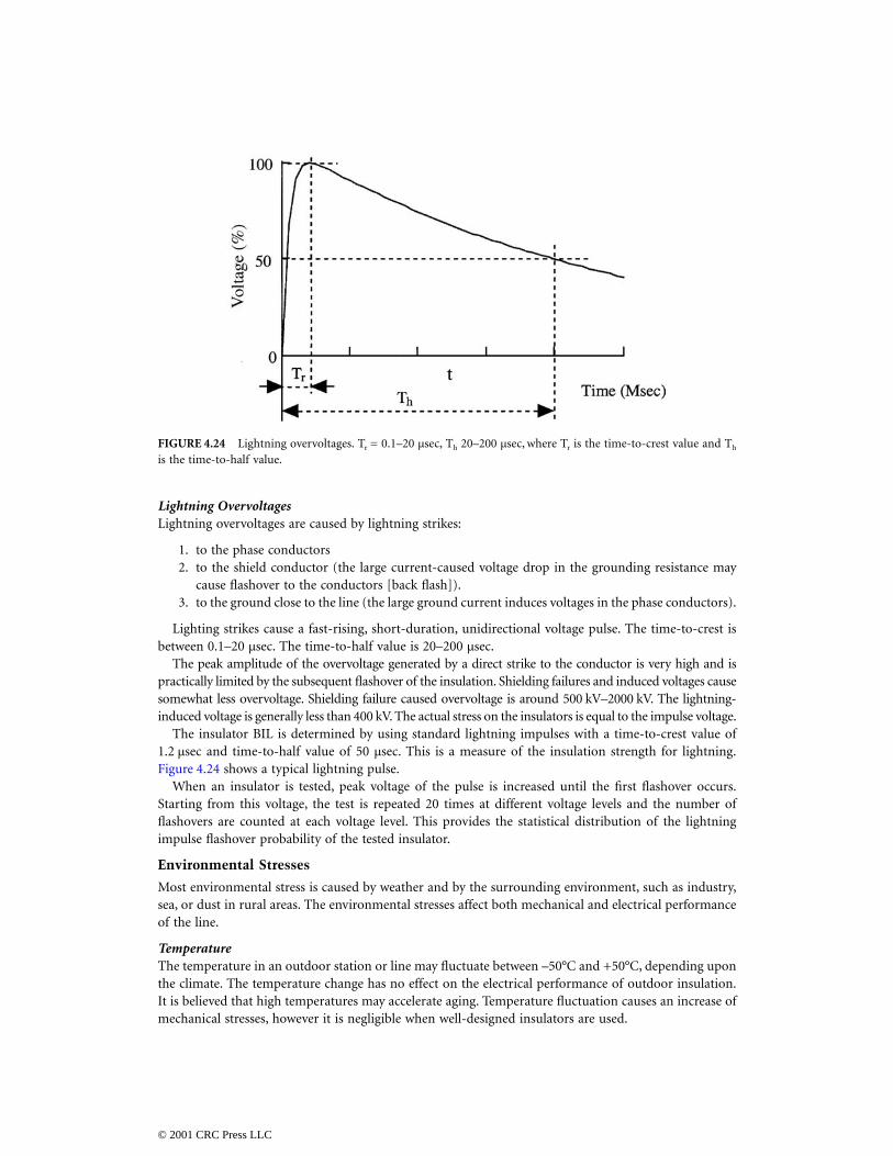
The insulator BIL is determined by using standard lightning impulses with a time-to-crest value of1.2 µsec and time-to-half value of 50 µsec. This is a measure of the insulation strength for lightning.Figure 4.24 shows a typical lightning pulse.

When an insulator is tested, peak voltage of the pulse is increased until the first flashover occurs.Starting from this voltage, the test is repeated 20 times at different voltage levels and the number offlashovers are counted at each voltage level. This provides the statistical distribution of the lightningimpulse flashover probability of the tested insulator.

Environmental Stresses

Most environmental stress is caused by weather and by the surrounding environment, such as industry,sea, or dust in rural areas. The environmental stresses affect both mechanical and electrical performanceof the line.

TemperatureThe temperature in an outdoor station or line may fluctuate between –50°C and +50°C, depending uponthe climate. The temperature change has no effect on the electrical performance of outdoor insulation.It is believed that high temperatures may accelerate aging. Temperature fluctuation causes an increase ofmechanical stresses, however it is negligible when well-designed insulators are used.

FIGURE 4.24 Lightning overvoltages. Tr = 0.1–20 µsec, Th 20–200 µsec, where Tr is the time-to-crest value and Th

is the time-to-half value.


UV RadiationUV radiation accelerates the aging of nonceramic composite insulators, but has no effect on porcelainand glass insulators. Manufacturers use fillers and modified chemical structures of the insulating materialto minimize the UV sensitivity.

RainRain wets porcelain insulator surfaces and produces a thin conducting layer most of the time. This reducesthe flashover voltage of the insulators. As an example, a 230-kV line may use an insulator string with12 standard ball-and-socket-type insulators. Dry flashover voltage of this string is 665 kV and the wetflashover voltage is 502 kV. The percentage reduction is about 25%.

Nonceramic polymer insulators have a water-repellent hydrophobic surface that reduces the effects ofrain. As an example, with a 230-kV composite insulator, dry flashover voltage is 735 kV and wet flashovervoltage is 630 kV. The percentage reduction is about 15%. The insulator’s wet flashover voltage must behigher than the maximum temporary overvoltage.

IcingIn industrialized areas, conducting water may form ice due to water-dissolved industrial pollution. Anexample is the ice formed from acid rain water. Ice deposits form bridges across the gaps in an insulatorstring that result in a solid surface. When the sun melts the ice, a conducting water layer will bridge theinsulator and cause flashover at low voltages. Melting ice-caused flashover has been reported in theQuebec and Montreal areas.

PollutionWind drives contaminant particles into insulators. Insulators produce turbulence in airflow, which resultsin the deposition of particles on their surfaces. The continuous depositing of the particles increases thethickness of these deposits. However, the natural cleaning effect of wind, which blows loose particlesaway, limits the growth of deposits. Occasionally, rain washes part of the pollution away. The continuousdepositing and cleaning produces a seasonal variation of the pollution on the insulator surfaces. However,after a long time (months, years), the deposits are stabilized and a thin layer of solid deposit will coverthe insulator. Because of the cleaning effects of rain, deposits are lighter on the top of the insulators andheavier on the bottom. The development of a continuous pollution layer is compounded by chemicalchanges. As an example, in the vicinity of a cement factory, the interaction between the cement and waterproduces a tough, very sticky layer. Around highways, the wear of car tires produces a slick, tar-likecarbon deposit on the insulator’s surface.

Moisture, fog, and dew wet the pollution layer, dissolve the salt, and produce a conducting layer, whichin turn reduces the flashover voltage. The pollution can reduce the flashover voltage of a standard insulatorstring by about 20–25%.

Near the ocean, wind drives salt water onto insulator surfaces, forming a conducting salt-water layerwhich reduces the flashover voltage. The sun dries the pollution during the day and forms a white saltlayer. This layer is washed off even by light rain and produces a wide fluctuation in pollution levels.

The Equivalent Salt Deposit Density (ESDD) describes the level of contamination in an area. EquivalentSalt Deposit Density is measured by periodically washing down the pollution from selected insulatorsusing distilled water. The resistivity of the water is measured and the amount of salt that produces thesame resistivity is calculated. The obtained mg value of salt is divided by the surface area of the insulator. Thisnumber is the ESDD. The pollution severity of a site isdescribed by the average ESDD value, which is deter-mined by several measurements.

Table 4.2 shows the criteria for defining site severity.The contamination level is light or very light in most

parts of the U.S. and Canada. Only the seashores andheavily industrialized regions experience heavy pollution.

TABLE 4.2 Site Severity (IEEE Definitions)

Description ESDD (mg/cm2)

Very light 0–0.03Light 0.03–0.06Moderate 0.06–0.1Heavy <0.1


Typically, the pollution level is very high in Florida and on the southern coast of California. Heavyindustrial pollution occurs in the industrialized areas and near large highways. Table 4.3 gives a summaryof the different sources of pollution.

The flashover voltage of polluted insulators has been measured in laboratories. The correlation betweenthe laboratory results and field experience is weak. The test results provide guidance, but insulators areselected using practical experience.

AltitudeThe insulator’s flashover voltage is reduced as altitude increases. Above 1500 feet, an increase in thenumber of insulators should be considered. A practical rule is a 3% increase of clearance or insulatorstrings’ length per 1000 ft as the elevation increases.

Mechanical Stresses

Suspension insulators need to carry the weight of the conductors and the weight of occasional ice andwind loading.

In northern areas and in higher elevations, insulators and lines are frequently covered by ice in thewinter. The ice produces significant mechanical loads on the conductor and on the insulators. Thetransmission line insulators need to support the conductor’s weight and the weight of the ice in theadjacent spans. This may increase the mechanical load by 20–50%.

The wind produces a horizontal force on the line conductors. This horizontal force increases themechanical load on the line. The wind-force-produced load has to be added vectorially to the weight-produced forces. The design load will be the larger of the combined wind and weight, or ice and wind load.

The dead-end insulators must withstand the longitudinal load, which is higher than the simple weightof the conductor in the half span.

A sudden drop in the ice load from the conductor produces large-amplitude mechanical oscillations,which cause periodic oscillatory insulator loading (stress changes from tension to compression and back).

The insulator’s one-minute tension strength is measured and used for insulator selection. In addition,each cap-and-pin or ball-and-socket insulator is loaded mechanically for one minute and simultaneouslyenergized. This mechanical and electrical (M&E) value indicates the quality of insulators. The maximumload should be around 50% of the M&E load.

The Bonneville Power Administration uses the following practical relation to determine the requiredM&E rating of the insulators.

1. M&E > 5∗ Bare conductor weight/span2. M&E > Bare conductor weight + Weight of 3.81 cm (1.5 in) of ice on the conductor (3 lb/sq ft)3. M&E > 2∗ (Bare conductor weight + Weight of 0.63 cm (1/4 in) of ice on the conductor and

loading from a wind of 1.8 kg/sq ft (4 lb/sq ft)

The required M&E value is calculated from all equations above and the largest value is used.

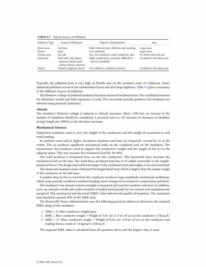
TABLE 4.3 Typical Sources of Pollution

Pollution Type Source of Pollutant Deposit Characteristics Area

Rural areas Soil dust High resitivity layer, effective rain washing Large areasDesert Sand Low resistivity Large areasCoastal area Sea salt Very low resistivity, easily washed by rain 10–20 km from the seaIndustrial Steel mill, coke plants,

chemical plants, gene-rating stations, quarries

High conductivity, extremely difficult to remove, insoluble

Localized to the plant area

Mixed Industry, highway, desert Very adhesive, medium resistivity Localized to the plant area


Ceramic (Porcelain and Glass) Insulators

Materials

Porcelain is the most frequently used material for insulators. Insulators are made of wet, processedporcelain. The fundamental materials used are a mixture of feldspar (35%), china clay (28%), flint (25%),ball clay (10%), and talc (2%). The ingredients are mixed with water. The resulting mixture has theconsistency of putty or paste and is pressed into a mold to form a shell of the desired shape. The alternativemethod is formation by extrusion bars that are machined into the desired shape. The shells are driedand dipped into a glaze material. After glazing, the shells are fired in a kiln at about 1200°C. The glazeimproves the mechanical strength and provides a smooth, shiny surface. After a cooling-down period,metal fittings are attached to the porcelain with Portland cement.

Toughened glass is also frequently used for insulators. The melted glass is poured into a mold to formthe shell. Dipping into hot and cold baths cools the shells. This thermal treatment shrinks the surface ofthe glass and produces pressure on the body, which increases the mechanical strength of the glass. Suddenmechanical stresses, such as a blow by a hammer or bullets, will break the glass into small pieces. Themetal end-fitting is attached by alumina cement.

Insulator Strings

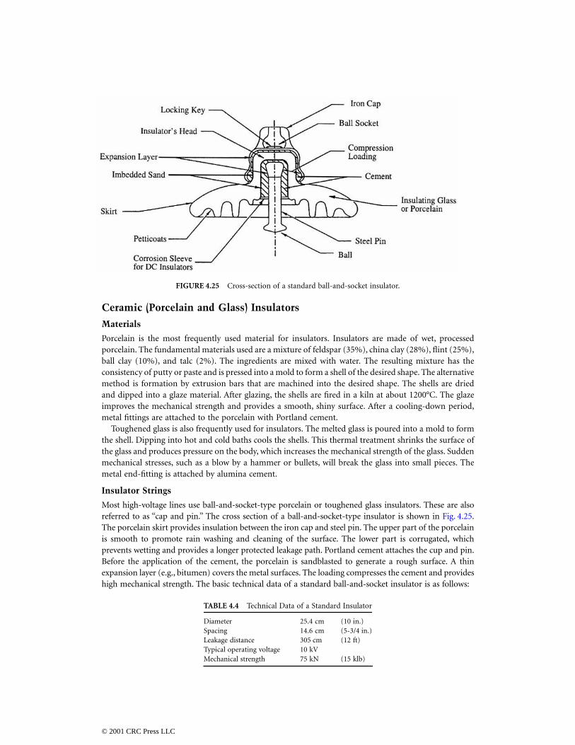
Most high-voltage lines use ball-and-socket-type porcelain or toughened glass insulators. These are alsoreferred to as “cap and pin.” The cross section of a ball-and-socket-type insulator is shown in Fig. 4.25.The porcelain skirt provides insulation between the iron cap and steel pin. The upper part of the porcelainis smooth to promote rain washing and cleaning of the surface. The lower part is corrugated, whichprevents wetting and provides a longer protected leakage path. Portland cement attaches the cup and pin.Before the application of the cement, the porcelain is sandblasted to generate a rough surface. A thinexpansion layer (e.g., bitumen) covers the metal surfaces. The loading compresses the cement and provideshigh mechanical strength. The basic technical data of a standard ball-and-socket insulator is as follows:

FIGURE 4.25 Cross-section of a standard ball-and-socket insulator.

TABLE 4.4 Technical Data of a Standard Insulator

Diameter 25.4 cm (10 in.)Spacing 14.6 cm (5-3/4 in.)Leakage distance 305 cm (12 ft)Typical operating voltage 10 kVMechanical strength 75 kN (15 klb)


The metal parts are designed to fail before the porcelain fails as the mechanical load increases. Thisacts as a mechanical fuse protecting the tower structure.

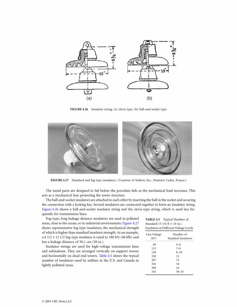
The ball-and-socket insulators are attached to each other by inserting the ball in the socket and securingthe connection with a locking key. Several insulators are connected together to form an insulator string.Figure 4.26 shows a ball-and-socket insulator string and the clevis-type string, which is used less fre-quently for transmission lines.

Fog-type, long leakage distance insulators are used in pollutedareas, close to the ocean, or in industrial environments. Figure 4.27shows representative fog-type insulators, the mechanical strengthof which is higher than standard insulator strength. As an example,a 6 1/2 × 12 1/2 fog-type insulator is rated to 180 kN (40 klb) andhas a leakage distance of 50.1 cm (20 in.).

Insulator strings are used for high-voltage transmission linesand substations. They are arranged vertically on support towersand horizontally on dead-end towers. Table 4.5 shows the typicalnumber of insulators used by utilities in the U.S. and Canada inlightly polluted areas.

FIGURE 4.26 Insulator string: (a) clevis type, (b) ball-and-socket type.

FIGURE 4.27 Standard and fog-type insulators. (Courtesy of Sediver, Inc., Nanterre Cedex, France.)

TABLE 4.5 Typical Number of Standard (5-1/4 ft × 10 in.) Insulators at Different Voltage Levels

Line Voltage(kV)

Number of Standard Insulators

69 4–6115 7–9138 8–10230 12287 15345 18500 24765 30–35


Post-Type Insulators

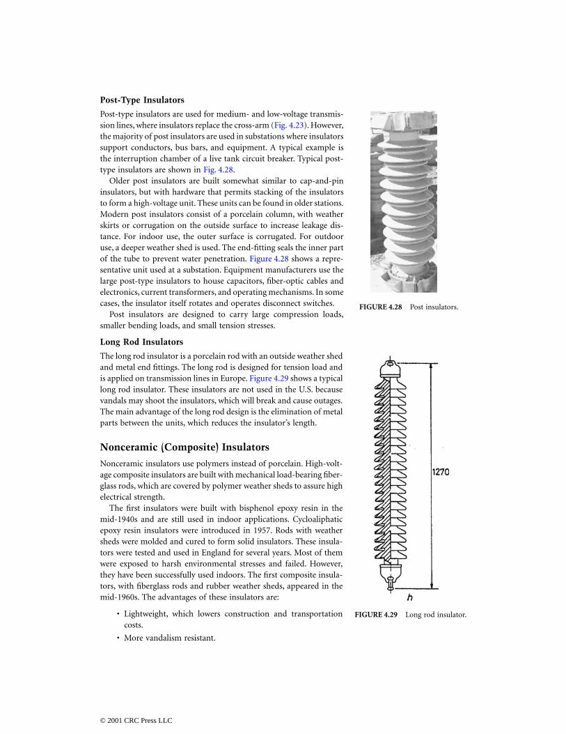
Post-type insulators are used for medium- and low-voltage transmis-sion lines, where insulators replace the cross-arm (Fig. 4.23). However,the majority of post insulators are used in substations where insulatorssupport conductors, bus bars, and equipment. A typical example isthe interruption chamber of a live tank circuit breaker. Typical post-type insulators are shown in Fig. 4.28.

Older post insulators are built somewhat similar to cap-and-pininsulators, but with hardware that permits stacking of the insulatorsto form a high-voltage unit. These units can be found in older stations.Modern post insulators consist of a porcelain column, with weatherskirts or corrugation on the outside surface to increase leakage dis-tance. For indoor use, the outer surface is corrugated. For outdooruse, a deeper weather shed is used. The end-fitting seals the inner partof the tube to prevent water penetration. Figure 4.28 shows a repre-sentative unit used at a substation. Equipment manufacturers use thelarge post-type insulators to house capacitors, fiber-optic cables andelectronics, current transformers, and operating mechanisms. In somecases, the insulator itself rotates and operates disconnect switches.

Post insulators are designed to carry large compression loads,smaller bending loads, and small tension stresses.

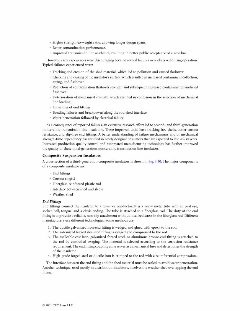
Long Rod Insulators

The long rod insulator is a porcelain rod with an outside weather shedand metal end fittings. The long rod is designed for tension load andis applied on transmission lines in Europe. Figure 4.29 shows a typicallong rod insulator. These insulators are not used in the U.S. becausevandals may shoot the insulators, which will break and cause outages.The main advantage of the long rod design is the elimination of metalparts between the units, which reduces the insulator’s length.

Nonceramic (Composite) Insulators

Nonceramic insulators use polymers instead of porcelain. High-volt-age composite insulators are built with mechanical load-bearing fiber-glass rods, which are covered by polymer weather sheds to assure highelectrical strength.

The first insulators were built with bisphenol epoxy resin in themid-1940s and are still used in indoor applications. Cycloaliphaticepoxy resin insulators were introduced in 1957. Rods with weathersheds were molded and cured to form solid insulators. These insula-tors were tested and used in England for several years. Most of themwere exposed to harsh environmental stresses and failed. However,they have been successfully used indoors. The first composite insula-tors, with fiberglass rods and rubber weather sheds, appeared in themid-1960s. The advantages of these insulators are:

• Lightweight, which lowers construction and transportationcosts.

• More vandalism resistant.

FIGURE 4.28 Post insulators.

FIGURE 4.29 Long rod insulator.


• Higher strength-to-weight ratio, allowing longer design spans.

• Better contamination performance.

• Improved transmission line aesthetics, resulting in better public acceptance of a new line.

However, early experiences were discouraging because several failures were observed during operation.Typical failures experienced were:

• Tracking and erosion of the shed material, which led to pollution and caused flashover.

• Chalking and crazing of the insulator’s surface, which resulted in increased contaminant collection,arcing, and flashover.

• Reduction of contamination flashover strength and subsequent increased contamination-inducedflashover.

• Deterioration of mechanical strength, which resulted in confusion in the selection of mechanicalline loading.

• Loosening of end fittings.

• Bonding failures and breakdowns along the rod-shed interface.

• Water penetration followed by electrical failure.

As a consequence of reported failures, an extensive research effort led to second- and third-generationnonceramic transmission line insulators. These improved units have tracking free sheds, better coronaresistance, and slip-free end fittings. A better understanding of failure mechanisms and of mechanicalstrength-time dependency has resulted in newly designed insulators that are expected to last 20–30 years.Increased production quality control and automated manufacturing technology has further improvedthe quality of these third-generation nonceramic transmission line insulators.

Composite Suspension Insulators

A cross-section of a third-generation composite insulators is shown in Fig. 4.30. The major componentsof a composite insulator are:

• End fittings

• Corona ring(s)

• Fiberglass-reinforced plastic rod

• Interface between shed and sleeve

• Weather shed

End FittingsEnd fittings connect the insulator to a tower or conductor. It is a heavy metal tube with an oval eye,socket, ball, tongue, and a clevis ending. The tube is attached to a fiberglass rod. The duty of the endfitting is to provide a reliable, non-slip attachment without localized stress in the fiberglass rod. Differentmanufacturers use different technologies. Some methods are:

1. The ductile galvanized iron-end fitting is wedged and glued with epoxy to the rod.2. The galvanized forged steel-end fitting is swaged and compressed to the rod.3. The malleable cast iron, galvanized forged steel, or aluminous bronze-end fitting is attached to

the rod by controlled swaging. The material is selected according to the corrosion resistancerequirement. The end fitting coupling zone serves as a mechanical fuse and determines the strengthof the insulator.

4. High-grade forged steel or ductile iron is crimped to the rod with circumferential compression.

The interface between the end fitting and the shed material must be sealed to avoid water penetration.Another technique, used mostly in distribution insulators, involves the weather shed overlapping the endfitting.


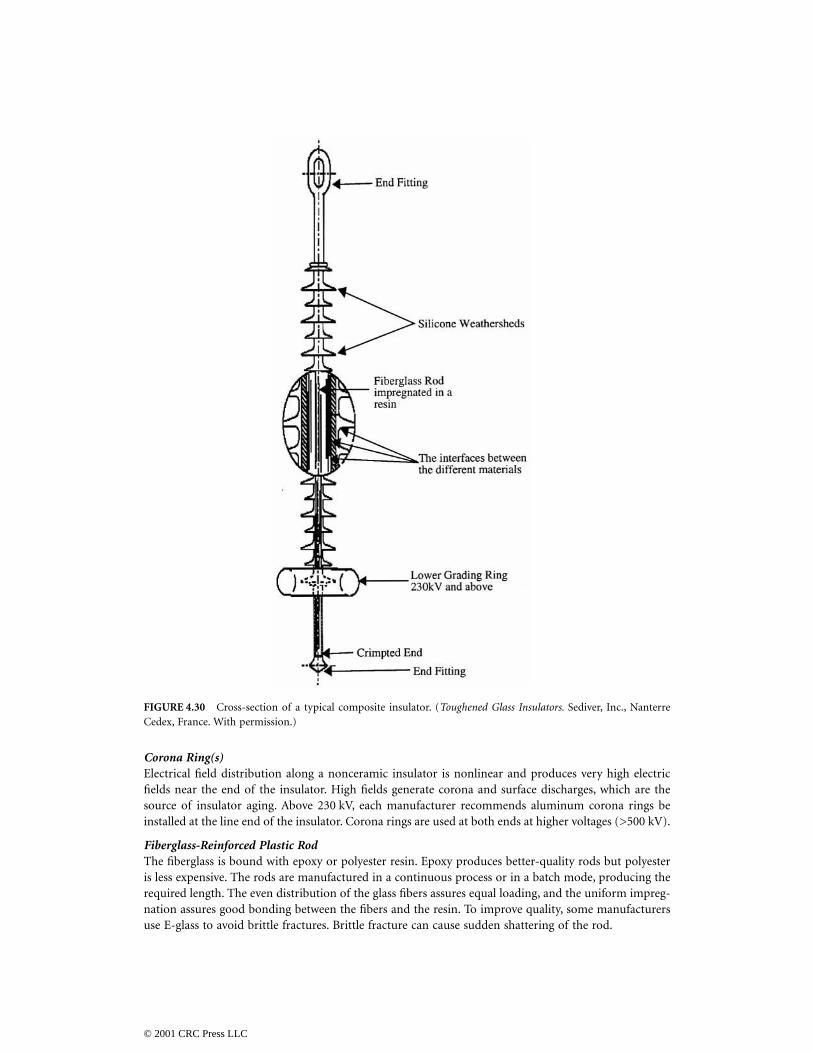
Corona Ring(s)Electrical field distribution along a nonceramic insulator is nonlinear and produces very high electricfields near the end of the insulator. High fields generate corona and surface discharges, which are thesource of insulator aging. Above 230 kV, each manufacturer recommends aluminum corona rings beinstalled at the line end of the insulator. Corona rings are used at both ends at higher voltages (>500 kV).

Fiberglass-Reinforced Plastic RodThe fiberglass is bound with epoxy or polyester resin. Epoxy produces better-quality rods but polyesteris less expensive. The rods are manufactured in a continuous process or in a batch mode, producing therequired length. The even distribution of the glass fibers assures equal loading, and the uniform impreg-nation assures good bonding between the fibers and the resin. To improve quality, some manufacturersuse E-glass to avoid brittle fractures. Brittle fracture can cause sudden shattering of the rod.

FIGURE 4.30 Cross-section of a typical composite insulator. (Toughened Glass Insulators. Sediver, Inc., NanterreCedex, France. With permission.)


Interfaces Between Shed and Fiberglass RodInterfaces between the fiberglass rod and weather shed should have no voids. This requires an appropriateinterface material that assures bonding of the fiberglass rod and weather shed. The most frequently usedtechniques are:

1. The fiberglass rod is primed by an appropriate material to assure the bonding of the sheds.2. Silicon rubber or ethylene propylene diene monomer (EPDM) sheets are extruded onto the

fiberglass rod, forming a tube-like protective covering.3. The gap between the rod and the weather shed is filled with silicon grease, which eliminates voids.

Weather ShedAll high-voltage insulators use rubber weather sheds installed on fiberglass rods. The interface betweenthe weather shed, fiberglass rod, and the end fittings are carefully sealed to prevent water penetration.The most serious insulator failure is caused by water penetration to the interface.

The most frequently used weather shed technologies are:

1. Ethylene propylene copolymer (EPM) and silicon rubber alloys, where hydrated-alumina fillersare injected into a mold and cured to form the weather sheds. The sheds are threaded to thefiberglass rod under vacuum. The inner surface of the weather shed is equipped with O-ring typegrooves filled with silicon grease that seals the rod-shed interface. The gap between the end-fittingsand the sheds is sealed by axial pressure. The continuous slow leaking of the silicon at the weathershed junctions prevents water penetration.

2. High-temperature vulcanized silicon rubber (HTV) sleeves are extruded on the fiberglass surfaceto form an interface. The silicon rubber weather sheds are injection-molded under pressure andplaced onto the sleeved rod at a predetermined distance. The complete subassembly is vulcanizedat high temperatures in an oven. This technology permits the variation of the distance betweenthe sheds.

3. The sheds are directly injection-molded under high pressure and high temperature onto theprimed rod assembly. This assures simultaneous bonding to both the rod and the end-fittings.Both EPDM and silicon rubber are used. This one-piece molding assures reliable sealing againstmoisture penetration.

4. One piece of silicon or EPDM rubber shed is molded directly to the fiberglass rod. The rubbercontains fillers and additive agents to prevent tracking and erosion.

Composite Post Insulators

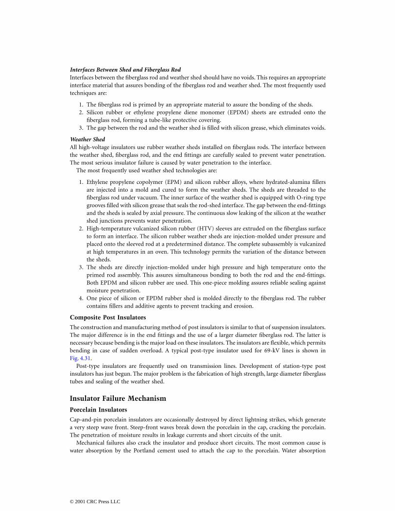
The construction and manufacturing method of post insulators is similar to that of suspension insulators.The major difference is in the end fittings and the use of a larger diameter fiberglass rod. The latter isnecessary because bending is the major load on these insulators. The insulators are flexible, which permitsbending in case of sudden overload. A typical post-type insulator used for 69-kV lines is shown inFig. 4.31.

Post-type insulators are frequently used on transmission lines. Development of station-type postinsulators has just begun. The major problem is the fabrication of high strength, large diameter fiberglasstubes and sealing of the weather shed.

Insulator Failure Mechanism

Porcelain Insulators

Cap-and-pin porcelain insulators are occasionally destroyed by direct lightning strikes, which generatea very steep wave front. Steep-front waves break down the porcelain in the cap, cracking the porcelain.The penetration of moisture results in leakage currents and short circuits of the unit.

Mechanical failures also crack the insulator and produce short circuits. The most common cause iswater absorption by the Portland cement used to attach the cap to the porcelain. Water absorption


expands the cement, which in turn cracks the porcelain. This reduces the mechanical strength, whichmay cause separation and line dropping.

Short circuits of the units in an insulator string reduce the electrical strength of the string, which maycause flashover in polluted conditions.

Glass insulators use alumina cement, which reduces water penetration and the head-cracking problem.A great impact, such as a bullet, can shatter the shell, but will not reduce the mechanical strength of theunit.

The major problem with the porcelain insulators is pollution, which may reduce the flashover voltageunder the rated voltages. Fortunately, most areas of the U.S. are lightly polluted. However, some areaswith heavy pollution experience flashover regularly.

Insulator Pollution

Insulation pollution is a major cause of flashovers and of long-term service interruptions. Lightning-caused flashovers produce short circuits. The short circuit current is interrupted by the circuit breakerand the line is reclosed successfully. The line cannot be successfully reclosed after pollution-causedflashover because the contamination reduces the insulation’s strength for a long time. Actually, theinsulator must dry before the line can be reclosed.

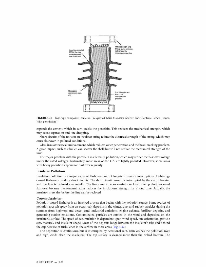
Ceramic InsulatorsPollution-caused flashover is an involved process that begins with the pollution source. Some sources ofpollution are: salt spray from an ocean, salt deposits in the winter, dust and rubber particles during thesummer from highways and desert sand, industrial emissions, engine exhaust, fertilizer deposits, andgenerating station emissions. Contaminated particles are carried in the wind and deposited on theinsulator’s surface. The speed of accumulation is dependent upon wind speed, line orientation, particlesize, material, and insulator shape. Most of the deposits lodge between the insulator’s ribs and behindthe cap because of turbulence in the airflow in these areas (Fig. 4.32).

The deposition is continuous, but is interrupted by occasional rain. Rain washes the pollution awayand high winds clean the insulators. The top surface is cleaned more than the ribbed bottom. The

FIGURE 4.31 Post-type composite insulator. (Toughened Glass Insulators. Sediver, Inc., Nanterre Cedex, France.With permission.)


horizontal and V strings are cleaned better by the rain than the I strings. The deposit on the insulatorforms a well-dispersed layer and stabilizes around an average value after longer exposure times. However,this average value varies with the changing of the seasons.

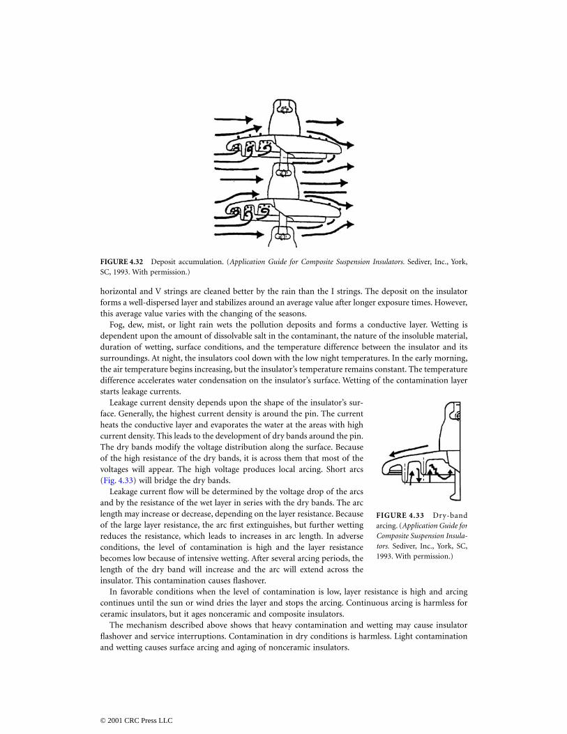
Fog, dew, mist, or light rain wets the pollution deposits and forms a conductive layer. Wetting isdependent upon the amount of dissolvable salt in the contaminant, the nature of the insoluble material,duration of wetting, surface conditions, and the temperature difference between the insulator and itssurroundings. At night, the insulators cool down with the low night temperatures. In the early morning,the air temperature begins increasing, but the insulator’s temperature remains constant. The temperaturedifference accelerates water condensation on the insulator’s surface. Wetting of the contamination layerstarts leakage currents.

Leakage current density depends upon the shape of the insulator’s sur-face. Generally, the highest current density is around the pin. The currentheats the conductive layer and evaporates the water at the areas with highcurrent density. This leads to the development of dry bands around the pin.The dry bands modify the voltage distribution along the surface. Becauseof the high resistance of the dry bands, it is across them that most of thevoltages will appear. The high voltage produces local arcing. Short arcs(Fig. 4.33) will bridge the dry bands.

Leakage current flow will be determined by the voltage drop of the arcsand by the resistance of the wet layer in series with the dry bands. The arclength may increase or decrease, depending on the layer resistance. Becauseof the large layer resistance, the arc first extinguishes, but further wettingreduces the resistance, which leads to increases in arc length. In adverseconditions, the level of contamination is high and the layer resistancebecomes low because of intensive wetting. After several arcing periods, thelength of the dry band will increase and the arc will extend across theinsulator. This contamination causes flashover.

In favorable conditions when the level of contamination is low, layer resistance is high and arcingcontinues until the sun or wind dries the layer and stops the arcing. Continuous arcing is harmless forceramic insulators, but it ages nonceramic and composite insulators.

The mechanism described above shows that heavy contamination and wetting may cause insulatorflashover and service interruptions. Contamination in dry conditions is harmless. Light contaminationand wetting causes surface arcing and aging of nonceramic insulators.

FIGURE 4.32 Deposit accumulation. (Application Guide for Composite Suspension Insulators. Sediver, Inc., York,SC, 1993. With permission.)

FIGURE 4.33 Dry-bandarcing. (Application Guide forComposite Suspension Insula-tors. Sediver, Inc., York, SC,1993. With permission.)


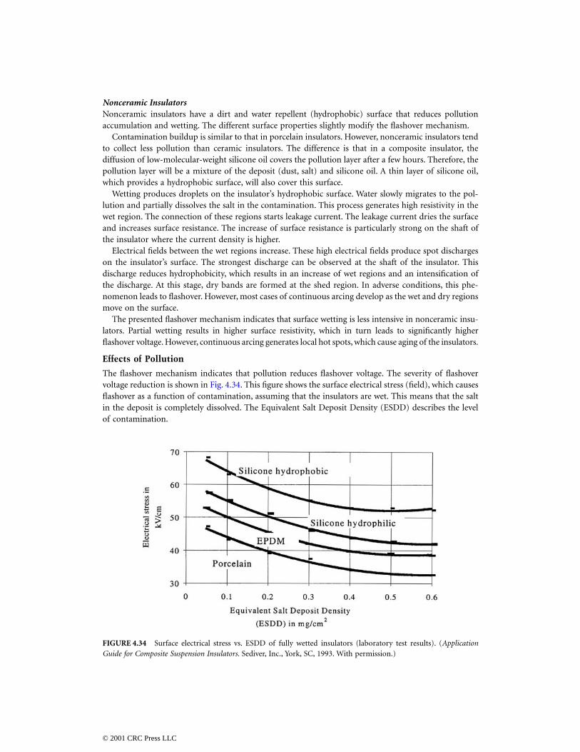
Nonceramic InsulatorsNonceramic insulators have a dirt and water repellent (hydrophobic) surface that reduces pollutionaccumulation and wetting. The different surface properties slightly modify the flashover mechanism.

Contamination buildup is similar to that in porcelain insulators. However, nonceramic insulators tendto collect less pollution than ceramic insulators. The difference is that in a composite insulator, thediffusion of low-molecular-weight silicone oil covers the pollution layer after a few hours. Therefore, thepollution layer will be a mixture of the deposit (dust, salt) and silicone oil. A thin layer of silicone oil,which provides a hydrophobic surface, will also cover this surface.

Wetting produces droplets on the insulator’s hydrophobic surface. Water slowly migrates to the pol-lution and partially dissolves the salt in the contamination. This process generates high resistivity in thewet region. The connection of these regions starts leakage current. The leakage current dries the surfaceand increases surface resistance. The increase of surface resistance is particularly strong on the shaft ofthe insulator where the current density is higher.

Electrical fields between the wet regions increase. These high electrical fields produce spot dischargeson the insulator’s surface. The strongest discharge can be observed at the shaft of the insulator. Thisdischarge reduces hydrophobicity, which results in an increase of wet regions and an intensification ofthe discharge. At this stage, dry bands are formed at the shed region. In adverse conditions, this phe-nomenon leads to flashover. However, most cases of continuous arcing develop as the wet and dry regionsmove on the surface.

The presented flashover mechanism indicates that surface wetting is less intensive in nonceramic insu-lators. Partial wetting results in higher surface resistivity, which in turn leads to significantly higherflashover voltage. However, continuous arcing generates local hot spots, which cause aging of the insulators.

Effects of Pollution

The flashover mechanism indicates that pollution reduces flashover voltage. The severity of flashovervoltage reduction is shown in Fig. 4.34. This figure shows the surface electrical stress (field), which causesflashover as a function of contamination, assuming that the insulators are wet. This means that the saltin the deposit is completely dissolved. The Equivalent Salt Deposit Density (ESDD) describes the levelof contamination.

FIGURE 4.34 Surface electrical stress vs. ESDD of fully wetted insulators (laboratory test results). (ApplicationGuide for Composite Suspension Insulators. Sediver, Inc., York, SC, 1993. With permission.)


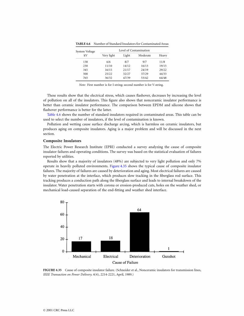
These results show that the electrical stress, which causes flashover, decreases by increasing the levelof pollution on all of the insulators. This figure also shows that nonceramic insulator performance isbetter than ceramic insulator performance. The comparison between EPDM and silicone shows thatflashover performance is better for the latter.

Table 4.6 shows the number of standard insulators required in contaminated areas. This table can beused to select the number of insulators, if the level of contamination is known.

Pollution and wetting cause surface discharge arcing, which is harmless on ceramic insulators, butproduces aging on composite insulators. Aging is a major problem and will be discussed in the nextsection.

Composite Insulators

The Electric Power Research Institute (EPRI) conducted a survey analyzing the cause of compositeinsulator failures and operating conditions. The survey was based on the statistical evaluation of failuresreported by utilities.

Results show that a majority of insulators (48%) are subjected to very light pollution and only 7%operate in heavily polluted environments. Figure 4.35 shows the typical cause of composite insulatorfailures. The majority of failures are caused by deterioration and aging. Most electrical failures are causedby water penetration at the interface, which produces slow tracking in the fiberglass rod surface. Thistracking produces a conduction path along the fiberglass surface and leads to internal breakdown of theinsulator. Water penetration starts with corona or erosion-produced cuts, holes on the weather shed, ormechanical load-caused separation of the end-fitting and weather shed interface.

TABLE 4.6 Number of Standard Insulators for Contaminated Areas

System Voltage Level of Contamination

kV Very light Light Moderate Heavy

138 6/6 8/7 9/7 11/8230 11/10 14/12 16/13 19/15345 16/15 21/17 24/19 29/22500 25/22 32/27 37/29 44/33765 36/32 47/39 53/42 64/48

Note: First number is for I-string; second number is for V-string.

FIGURE 4.35 Cause of composite insulator failure. (Schneider et al., Nonceramic insulators for transmission lines,IEEE Transaction on Power Delivery, 4(4), 2214-2221, April, 1989.)


Most of the mechanical failures are caused by breakage of the fiberglass rods in the end fitting. Thisoccurs because of local stresses caused by inappropriate crimping. Another cause of mechanical failuresis brittle fracture. Brittle fracture is initiated by the penetration of water containing slight acid frompollution. The acid may be produced by electrical discharge and acts as a cathalizator, attacking the bondsand the glass fibers to produce a smooth fracture. The brittle fractures start at high mechanical stresspoints, many times in the end fitting.

Aging of Composite Insulators

Most technical work concentrates on the aging of nonceramic insulators and the development of testmethods that simulate the aging process. Transmission lines operate in a polluted atmosphere. Inevitably,insulators will become polluted after several months in operation. Fog and dew cause wetting and produceuneven voltage distribution, which results in surface discharge. Observations of transmission lines atnight by a light magnifier show that surface discharge occurs in nearly every line in wet conditions. UVradiation and surface discharge cause some level of deterioration after long-term operation. These arethe major causes of aging in composite insulators which also lead to the uncertainty of an insulator’slife span. If the deterioration process is slow, the insulator can perform well for a long period of time.This is true of most locations in the U.S. and Canada. However, in areas closer to the ocean or areaspolluted by industry, deterioration may be accelerated and insulator failure may occur after a few yearsof exposure. Surveys indicate that some insulators operate well for 18–20 years and others fail after afew months. An analysis of laboratory data and literature surveys permit the formulation of the followingaging hypothesis:

1. Wind drives dust and other pollutants into the composite insulator’s water-repellent surface. Thecombined effects of mechanical forces and UV radiation produces slight erosion of the surface,increasing surface roughness and permitting the slow buildup of contamination.

2. Diffusion drives polymers out of the bulk skirt material and embeds the contamination. A thinlayer of polymer will cover the contamination, assuring that the surface maintains hydrophobicity.

3. High humidity, fog, dew, or light rain produce droplets on the hydrophobic insulator surface.Droplets may roll down from steeper areas. In other areas, contaminants diffuse through the thinpolymer layer and droplets become conductive.

4. Contamination between the droplets is wetted slowly by the migration of water into the drycontaminant. This generates a high resistance layer and changes the leakage current from capacitiveto resistive.

5. The uneven distribution and wetting of the contaminant produces an uneven voltage stressdistribution along the surface. Corona discharge starts around the droplets at the high stress areas.Additional discharge may occur between the droplets.

6. The discharge consumes the thin polymer layer around the droplets and destroys hydrophobicity.7. The deterioration of surface hydrophobicity results in dispersion of droplets and the formation

of a continuous conductive layer in the high stress areas. This increases leakage current.8. Leakage current produces heating, which initiates local dry band formation.9. At this stage, the surface consists of dry regions, highly resistant conducting surfaces, and hydro-

phobic surfaces with conducting droplets. The voltage stress distribution will be uneven on thissurface.

10. Uneven voltage distribution produces arcing and discharges between the different dry bands. Thesecause further surface deterioration, loss of hydrophobicity, and the extension of the dry areas.

11. Discharge and local arcing produces surface erosion, which ages the insulator’s surface.12. A change in the weather, such as the sun rising, reduces the wetting. As the insulator dries, the

discharge diminishes.13. The insulator will regain hydrophobicity if the discharge-free dry period is long enough. Typically,

silicon rubber insulators require 6–8 h; EPDM insulators require 12–15 h to regain hydrophobicity.


14. Repetition of the described procedure produces erosion on the surface. Surface roughness increasesand contamination accumulation accelerates aging.

15. Erosion is due to discharge-initiated chemical reactions and a rise in local temperature. Surfacetemperature measurements, by temperature indicating point, show local hot-spot temperaturesbetween 260°C and 400°C during heavy discharge.

The presented hypothesis is supported by the observation that the insulator life spans in dry areas arelonger than in areas with a wetter climate. Increasing contamination levels reduce an insulator’s life span.The hypothesis is also supported by observed beneficial effects of corona rings on insulator life.

DeTourreil et al. (1990) reported that aging reduces the insulator’s contamination flashover voltage.Different types of insulators were exposed to light natural contamination for 36–42 months at two differentsites. The flashover voltage of these insulators was measured using the “quick flashover salt fog” technique,before and after the natural aging. The quick flashover salt fog procedure subjects the insulators to saltfog (80 kg/m3 salinity). The insulators are energized and flashed over 5–10 times. Flashover was obtainedby increasing the voltage in 3% steps every 5 min from 90% of the estimated flashover value until flashover.The insulators were washed, without scrubbing, before the salt fog test. The results show that flashovervoltage on the new insulators was around 210 kV and the aged insulators flashed over around 184–188 kV.The few years of exposure to light contamination caused a 10–15% reduction of salt fog flashover voltage.

Natural aging and a follow-up laboratory investigation indicated significant differences between theperformance of insulators made by different manufacturers. Natural aging caused severe damage on someinsulators and no damage at all on others.

Methods for Improving Insulator Performance

Contamination caused flashovers produce frequent outages in severely contaminated areas. Lines closerto the ocean are in more danger of becoming contaminated. Several countermeasures have been proposedto improve insulator performance. The most frequently used methods are:

1. Increasing leakage distance by increasing the number of units or by using fog-type insulators.The disadvantages of the larger number of insulators are that both the polluted and the impulseflashover voltages increase. The latter jeopardizes the effectiveness of insulation coordinationbecause of the increased strike distance, which increases the overvoltages at substations.

2. Application insulators are covered with a semiconducting glaze. A constant leakage current flowsthrough the semiconducting glaze. This current heats the insulator’s surface and reduces themoisture of the pollution. In addition, the resistive glaze provides an alternative path when drybands are formed. The glaze shunts the dry bands and reduces or eliminates surface arcing. Theresistive glaze is exceptionally effective near the ocean.

3. Periodic washing of the insulators with high-pressure water. The transmission lines are washedby a large truck carrying water and pumping equipment. Trained personnel wash the insulatorsby aiming the water spray toward the strings. Substations are equipped with permanent washingsystems. High-pressure nozzles are attached to the towers and water is supplied from a centralpumping station. Safe washing requires spraying large amounts of water at the insulators in ashort period of time. Fast washing prevents the formation of dry bands and pollution-causedflashover. However, major drawbacks of this method include high installation and operationalcosts.

4. Periodic cleaning of the insulators by high pressure driven abrasive material, such as groundcorn cobs or walnut shells. This method provides effective cleaning, but cleaning of the residualfrom the ground is expensive and environmentally undesirable.

5. Replacement of porcelain insulators with nonceramic insulators. Nonceramic insulators havebetter pollution performance, which eliminates short-term pollution problems at most sites.However, insulator aging may affect the long-term performance.


6. Covering the insulators with a thin layer of room-temperature vulcanized (RTV) silicon rubbercoating. This coating has a hydrophobic and dirt-repellent surface, with pollution performancesimilar to nonceramic insulators. Aging causes erosion damage to the thin layer after 5–10 yearsof operation. When damage occurs, it requires surface cleaning and a reapplication of the coating.Cleaning by hand is very labor intensive. The most advanced method is cleaning with high pressuredriven abrasive materials like ground corn cobs or walnut shells. The coating is sprayed on thesurface using standard painting techniques.

7. Covering the insulators with a thin layer of petroleum or silicon grease. Grease provides ahydrophobic surface and absorbs the pollution particles. After one or two years of operation, thegrease saturates the particles and it must be replaced. This requires cleaning of the insulator andapplication of the grease, both by hand. Because of the high cost and short life span of the grease,it is not used anymore.

References

Application Guide for Composite Suspension Insulators, Sediver Inc., York, SC, 1993.DeTourreil, C.H. and Lambeth, P.J., Aging of composite insulators: Simulation by electrical tests, IEEE

Trans. on Power Delivery, 5(3), 1558-1567, July, 1990.Fink, D.G. and Beaty, H.W., Standard Handbook for Electrical Engineers, 11th ed., McGraw-Hill, New

York, 1978.Gorur, R.S., Karady, G.G., Jagote, A., Shah, M., and Yates, A., Aging in silicon rubber used for outdoor

insulation, IEEE Transaction on Power Delivery, 7(2), 525-532, March, 1992.Hall, J.F., History and bibliography of polymeric insulators for outdoor application, IEEE Transaction on

Power Delivery, 8(1), 376-385, January, 1993.Karady, G.G., Outdoor insulation, Proceedings of the Sixth International Symposium on High Voltage

Engineering, New Orleans, LA, September, 1989, 30.01-30.08.Karady, G.G., Rizk, F.A.M., and Schneider, H.H., Review of CIGRE and IEEE Research into Pollution

Performance of Nonceramic Insulators: Field Aging Effect and Laboratory Test Techniques, inInternational Conference on Large Electric High Tension Systems (CIGRE), Group 33, (33-103), Paris,1-8, August, 1994.

Looms, J.S.T., Insulators for High Voltages, Peter Peregrinus Ltd., London, 1988.Schneider, H., Hall, J.F., Karady, G., and Rendowden, J., Nonceramic insulators for transmission lines,

IEEE Transaction on Power Delivery, 4(4), 2214-2221, April, 1989.Toughened Glass Insulators. Sediver Inc., Nanterre Cedex, France.Transmission Line Reference Book (345 kV and Above), 2nd ed., EL 2500 Electric Power Research Institute

(EPRI), Palo Alto, CA, 1987.

4.4 Transmission Line Construction and Maintenance

Wilford Caulkins and Kristine Buchholz

The information herein was derived from personal observation and participation in the construction ofoverhead transmission lines for over 35 years. Detailed information, specific tools and equipment havebeen provided previously and are available in IEEE Standard 524-1992 and IEEE Standard 524A-1993.

The purpose of this section is to give a general overview of the steps that are necessary in the planningand construction of a typical overhead transmission line, to give newcomers to the trade a general formatto follow, and assist transmission design engineers in understanding how such lines are built.

Stringing overhead conductors in transmission is a very specialized type of construction requiringyears of experience, as well as equipment and tools that have been designed, tried, and proven to do thework. Because transmission of electrical current is normally at higher voltages (69 kV and above),conductors must be larger in diameter and span lengths must be longer than in normal distribution.


Although proximity to other energized lines may be limited on the right-of-way, extra care must beexercised to protect the conductor so that when energized, power loss and corona are not a problem.

There are four methods that can be used to install overhead transmission conductors:

1. Slack stringing2. Semi-tension stringing3. Full-tension stringing4. Helicopter stringing

Slack stringing can only be utilized if it is not necessary to keep the conductor off of the ground, andif no energized lines lie beneath the line being strung. In this method the pulling lines are pulled out onthe ground, threaded through the stringing blocks, and the conductor is pulled in with less tension thanis required to keep it off the ground. This is not considered to be an acceptable method when demandsinvolve maximum utilization of transmission requirements.

Semi-tension methods are merely an upgrading of slack stringing, but do not necessarily keep theconductor completely clear of the ground, or the lines used to pull.

Full-tension stringing is a method of installing the conductors and overhead groundwire in whichsufficient pulling capabilities on one end and tension capabilities on the other, keep the wires clear ofany obstacles during the movement of the conductor from the reel to its final sag position. This ensuresthat these current-carrying cables are “clipped” into the support clamps in the best possible condition,which is the ultimate goal of the work itself.

Stringing with helicopters, which is much more expensive per hour of work, can be much less expensivewhen extremely arduous terrain exists along the right-of-way and when proper pre-planning is utilized.Although pulling conductors themselves with a helicopter can be done, it is limited and normally notpractical. Maximum efficiency can be achieved when structures are set and pilot lines are pulled withthe helicopter, and then the conductor stringing is done in a conventional manner. Special tools (suchas stringing blocks) are needed if helicopters are used.

So that maximum protection of the conductor is realized and maximum safety of personnel is attained,properly designed and constructed tools and equipment are tantamount to a successful job. Because theinitial cost of these tools and equipment represent such a small percentage of the overall cost of theproject, the highest quality should be used, thus minimizing “down time” and possible failure duringthe course of construction.

Tools

Basic tools needed to construct overhead transmission lines are as follows:

1. Conductor blocks2. Overhead groundwire blocks3. Catch-off blocks4. Sagging blocks5. Pulling lines6. Pulling grips7. Catch-off grips8. Swivels9. Running boards

10. Conductor lifting hooks11. Hold-down blocks

Conductor blocks are made in the following configurations:

1. Single conductor2. Multiple conductor3. Multiversal type (can be converted from bundle to single, and vice versa)4. Helicopter


Conductor blocks should be large enough to properly accommodate the conductor and be lined witha resilient liner such as neoprene or polyurethane and constructed of lightweight, high-strength materials.Sheaves should be mounted on anti-friction ball bearings to reduce the tension required in stringing andfacilitate proper sagging. Conductor blocks are available for stringing single conductors or multipleconductors. Some are convertible, thus enhancing their versatility. When stringing multiple conductors,it is desirable to pull all conductors with a single pulling line so that all conductors in the bundle haveidentical tension history. The running board makes this possible. Pulling lines are divided into twocategories:

1. Steel cable2. Synthetic rope

Because of the extra high tension required in transmission line construction, steel pulling lines andpilot lines are most practical to use. Torque-resistant, stranded, and swagged cable are used so that ballbearing swivels can be utilized to prevent torque buildup from being transferred to the conductor. Somebraided or woven steel cables are also used. If synthetic ropes are utilized, the most important featuresshould include:

1. No torque2. Very minimum elongation3. No “kinking”4. Easily spliced5. High strength/small diameter6. Excellent dielectric properties

Stringing overhead groundwires does not normally require the care of current-carrying conductors.Most overhead groundwires are stranded steel construction and the use of steel wire with a fiber-opticcore for communications has become a common practice. Special care should be taken to ensure thatexcessive bending does not occur when erecting overhead groundwires with fiber-optic centers, such asOPT-GW (Optical Power Telecommunications — Ground Wire) and ADSS (All Dielectric Self-Support-ing Cable). Special instructions are available from the manufacturer, which specify minimum sheave andbullwheel diameter for construction. OPT-GW should be strung using an antirotational device to preventthe cable from twisting.

Equipment

Pullers are used to bring in the main pulling line. Multidrum pullers, called pilot line winders, are usedto tension string the heavy pulling cable.

Primary pullers are used to tension string the conductors. These pullers are either drum type orbullwheel type. The drum type is used more extensively in many areas of North America because thepuller and pulling cable are stored on one piece of equipment, but it is not practical in other areas becauseit is too heavy. Thus, the bullwheel type is used allowing the puller and pulling cable to be separatedonto two pieces of equipment. Also, the pulling cable can be separated into shorter lengths to allow easierhandling, especially if manual labor is preferred.

Tensioners should be bullwheel type using multigroove wheels for more control. Although V groovemachines are used on some lighter, smaller conductors, they are not recommended in transmission workbecause of the crushing effect on the conductor. Tensioners are either mounted on a truck or trailer.

Reel stands are used to carry the heavy reels of conductor and are equipped with brakes to hold “tailingtension” on the conductor as it is fed into the bullwheel tensioner. These stands are usually mounted ona trailer separated from the tensioner.

Helicopters are normally used to fly in a light line which can be used to pull in the heavier cable.


Procedures

Once the right-of-way has been cleared, the following are normal steps taken in construction:

1. Framing2. Pulling3. Pulling overhead groundwire up to sag and installation4. Pulling in main line with pilot line5. Stringing conductors6. Sagging conductors7. Clipping in conductors8. Installing spacer or spacer dampers where applicable

Framing normally consists of erecting poles, towers, or other structures, including foundations andanchors on guyed structures. It is desirable for the stringing blocks to be installed, with finger lines, onthe ground before structures are set, to eliminate an extra climb later. Helicopters are used to set structures,especially where rough terrain exists or right-of-way clearances are restricted.

Once structures are secure, overhead groundwire and pilot lines are pulled in together with a piece ofequipment such as a caterpillar or other track vehicle. A helicopter is also used to fly in these lines. Oncethe overhead groundwires are in place, they are sagged and secured, thus giving the structures morestability for the stringing of the conductors. This is especially important for guyed structures.

Normally the three pilot lines (typically 3/8 in. diameter swagged steel cable) pull in the heavier pullingline (typically 3/4 in. diameter or 7/8 in. diameter swagged steel) under tension. The main pulling lineis then attached to the conductor which is strung under full tension. Once the conductor is “caught off,”the main pulling line is returned for pulling of the next phase.

Once the conductors are in place, they are then brought up to final sag and clipped into the conductorclamps provided. If the conductor is a part of a bundle per phase, the spacers or spacer dampers areinstalled, using a spacer cart which is either pulled along from the ground or self-propelled.

Coordination between design engineers and construction personnel is very important in the planningand design of transmission lines. Although it is sometimes impossible to accommodate the most efficientcapabilities of the construction department (or line contractor), much time and money can be conservedif predesign meetings are held to discuss items such as the clearances needed for installing overheadgroundwire blocks, hardware equipped with “work” holes to secure lifting hooks or blocks, conductorreel sizes compatible with existing reel stands, length of pull most desirable, or towers equipped tofacilitate climbing.

For maximum safety of personnel constructing transmission lines, proper and effective groundingprocedures should be utilized. Grounding can be accomplished by:

1. adequate grounding of conductors being strung and pulling cables being used, or2. fully insulating equipment and operator, or3. isolating equipment and personnel.

All equipment, conductors, anchors, and structures within a defined work area must be bondedtogether and connected to the ground source. The recommended procedures of personnel protection arethe following:

1. Establish equipotential work zones.2. Select grounding equipment for the worst-case fault.3. Discontinue all work when the possibility of lightning exists which may affect the work site.

In addition to the grounding system, the best safety precaution is to treat all equipment as if it couldbecome energized.


Helicopters

As already mentioned, the use of helicopters is another option that is being chosen more frequently fortransmission system construction and maintenance. There are a wide variety of projects where helicoptersbecome involved, making the projects easier, safer, or more economical. When choosing any constructionor maintenance method, identify the work to be accomplished, analyze the potential safety aspects, listthe possible alternatives, and calculate the economics. Helicopters add a new dimension to this analyticalprocess by adding to the alternatives, frequently reducing the risks of accident or injury, and potentiallyreducing costs. The most critical consideration in the use of a helicopter is the ability to safely positionthe helicopter and line worker at the work location.

Conductor Stringing

Helicopters are used for conductor stringing on towers through the use of pilot lines. Special stringingblocks are installed at each tower and a helicopter is brought in and attached to a pilot line. The helicopterflies along the tower line and slips the pilot line in through each stringing block until it reaches the endof the set of towers for conductor pulling, where it disconnects and the pilot line is transferred to aground crew. The ground crew then proceeds to pull the conductor in the conventional manner (Caulkins,1987). The helicopter may also be used to monitor the conductor pulling and is readily available to assistif the conductor stalls at any tower location.

Structure and Material Setting

The most obvious use of helicopters is in the setting of new towers and structures. Helicopters arefrequently used in rough terrain to fly in the actual tower to a location where a ground crew is waitingto spot the structure into a preconstructed foundation. In addition, heavy material can be transportedto remote locations, as well as the construction crew.

The use of helicopters can be especially critical if the tower line is being replaced following a catastropheor failure. Frequently, roads and even construction paths are impassable or destroyed following naturaldisasters. Helicopters can carry crews and materials with temporary structures that can be erected withinhours to restore tower lines. Again, depending on the terrain and current conditions, whether the existingstructure is repaired or temporary tower structures are utilized, the helicopter is invaluable to carry inthe needed supplies and personnel.

Insulator Replacement

A frequent maintenance requirement on a transmission system is replacing insulators. This need isgenerated for various reasons, including line upgrading, gunshots, environmental damage, or defects inthe original insulator manufacturing. With close coordinated crews, helicopters can maximize the effi-ciency of the replacement project.

Crews are located at several towers to perform the actual insulator removal and installation. The crewswill do the required setup for a replacement, but the helicopter can be used to bring in the necessarytools and equipment. The crew removes the old insulator string and sets it to one side of the worklocation. When the crews are ready, the helicopter flies in the new insulator string to each tower. Thecrew on the tower detaches the new insulator string from the helicopter, positions it, and then attachesthe old string to the helicopter, which removes the string to the staging area. With a well-coordinatedteam of helicopters and experienced line workers, it is not unusual to achieve a production rate ofreplacing all insulators on four three-phase structures per crew per day. Under ideal conditions, crewsare able to replace the insulators on a structure in one hour (Buchholz, 1987).

Replacing Spacers

One of the first uses of helicopters in live-line work was the replacement of spacers in the early 1980s.This method was a historic step in live-line work since it circumvented the need for hot sticks or insulatedaerial lift devices.


The first projects involved a particular spacer wearing into the conductor strands, causing the sepa-ration of the conductor. Traditionally, the transmission line would have been de-energized, grounded,and either a line worker would have utilized a spacer cart to move out on the line to replace the spacer,or the line would have been lowered and the spacer replaced and the conductor strengthened. The obvioussafety dilemma was whether the conductor could support a line worker on a spacer cart or whether itwas physically able to withstand the tensions of lowering it to the ground. By utilizing a helicopter andbare-hand work methods, the spacers were able to be replaced and the conductor strengthened wherenecessary with full-tension compression splices while providing total safety to the line workers and acontinuous supply of energy over the transmission lines. One of the early projects achieved a replacementand installation of 25,000 spacers without a single accident or injury. A typical spacer replacementrequired about 45 sec, including the travel time between work locations (Buchholz, 1987).

Insulator Washing

Another common practice is to utilize helicopters for insulator washing. Again, this is a method thatallows for the line to remain energized during the process. The helicopter carries a water tank that isrefilled at a staging area near the work location. A hose and nozzle are attached to a structure on thehelicopter and are operated by a qualified line worker who directs the water spray and adequately cleansthe insulator string. Again, with the ease of access afforded by the helicopter, the speed of this operationcan result in a typical three-phase tower being cleaned in a few minutes.

Inspections

Helicopters are invaluable for tower line and structure inspections. Due to the ease of the practice andthe large number of inspections that can be accomplished, utilities have increased the amount of main-tenance inspections being done, thus promoting system reliability.

Helicopters typically carry qualified line workers who utilize stabilizing binoculars to visually inspectthe transmission tower for signs of rusting or weakness and the transmission hardware and conductorfor damage and potential failure. Infrared inspections and photographic imaging can also be accom-plished from the helicopter, either by mounting the cameras on the helicopter or through direct use bythe crew. During these inspections, the helicopter provides a comfortable situation for accomplishingthe necessary recording of specific information, tower locations, etc. In addition, inspections fromhelicopters are required following a catastrophic event or system failure. It is the only logical method ofquickly inspecting a transmission system for the exact location and extent of damage.

Helicopter Method Considerations

The ability to safely position a helicopter and worker at the actual work site is the most critical consid-eration when deciding if a helicopter method can be utilized for construction or maintenance. The terrainand weather conditions are obvious factors, as well as the physical spacing needed to position thehelicopter and worker in the proximity required for the work method. If live-line work methods are tobe utilized, the minimum approach distance required for energized line work must be calculated verycarefully for every situation. The geometry of each work structure, the geometry of the individualhelicopter, and the positioning of the helicopter and worker for the specific work method must beanalyzed. There are calculations that are available to analyze the approach distances (IEEE Task Force15.07.05.05, 1999).

When choosing between construction and maintenance work methods, the safety of the line workersis the first consideration. Depending on circumstances, a helicopter method may be the safest workmethod. Terrain has always been a primary reason for choosing helicopters to assist with projects sincethe ability to drive to each work site may not be possible. However, helicopters may still be the easiestand most economic alternative when the terrain is open and flat, especially when there are manyindividual tower locations that will be contacted. Although helicopters may seem to be expensive on aper person basis, the ability to quickly position workers and easily move material can drastically reduce


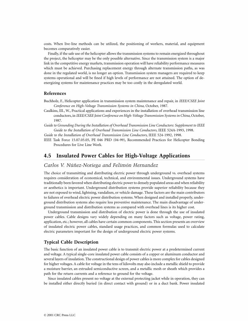
costs. When live-line methods can be utilized, the positioning of workers, material, and equipmentbecomes comparatively easier.

Finally, if the safe use of the helicopter allows the transmission systems to remain energized throughoutthe project, the helicopter may be the only possible alternative. Since the transmission system is a majorlink in the competitive energy markets, transmission operation will have reliability performance measureswhich must be achieved. Purchasing replacement energy through alternate transmission paths, as wasdone in the regulated world, is no longer an option. Transmission system managers are required to keepsystems operational and will be fined if high levels of performance are not attained. The option of de-energizing systems for maintenance practices may be too costly in the deregulated world.

References

Buchholz, F., Helicopter application in transmission system maintenance and repair, in IEEE/CSEE JointConference on High-Voltage Transmission Systems in China, October, 1987.

Caulkins, III., W., Practical applications and experiences in the installation of overhead transmission lineconductors, in IEEE/CSEE Joint Conference on High-Voltage Transmission Systems in China, October,1987.

Guide to Grounding During the Installation of Overhead Transmission Line Conductors: Supplement to IEEEGuide to the Installation of Overhead Transmission Line Conductors, IEEE 524A-1993, 1998.

Guide to the Installation of Overhead Transmission Line Conductors, IEEE 524-1992, 1998.IEEE Task Force 15.07.05.05, PE 046 PRD (04-99), Recommended Practices for Helicopter Bonding

Procedures for Live Line Work.

4.5 Insulated Power Cables for High-Voltage Applications

Carlos V. Núñez-Noriega and Felimón Hernandez

The choice of transmitting and distributing electric power through underground vs. overhead systemsrequires consideration of economical, technical, and environmental issues. Underground systems havetraditionally been favored when distributing electric power to densely populated areas and when reliabilityor aesthetics is important. Underground distribution systems provide superior reliability because theyare not exposed to wind, lightning, vandalism, or vehicle damage. These factors are the main contributorsto failures of overhead electric power distribution systems. When designed and installed properly, under-ground distribution systems also require less preventive maintenance. The main disadvantage of under-ground transmission and distribution systems as compared with overhead lines is its higher cost.

Underground transmission and distribution of electric power is done through the use of insulatedpower cables. Cable designs vary widely depending on many factors such as voltage, power rating,application, etc.; however, all cables have certain common components. This section presents an overviewof insulated electric power cables, standard usage practices, and common formulas used to calculateelectric parameters important for the design of underground electric power systems.

Typical Cable Description

The basic function of an insulated power cable is to transmit electric power at a predetermined currentand voltage. A typical single-core insulated power cable consists of a copper or aluminum conductor andseveral layers of insulation. The constructional design of power cables is more complex for cables designedfor higher voltages. A cable for voltage in the tens of kilovolts may also include a metallic shield to providea moisture barrier, an extruded semiconductive screen, and a metallic mesh or sheath which provides apath for the return currents and a reference to ground for the voltage.

Since insulated cables present no voltage at the external protecting jacket while in operation, they canbe installed either directly buried (in direct contact with ground) or in a duct bank. Power insulated


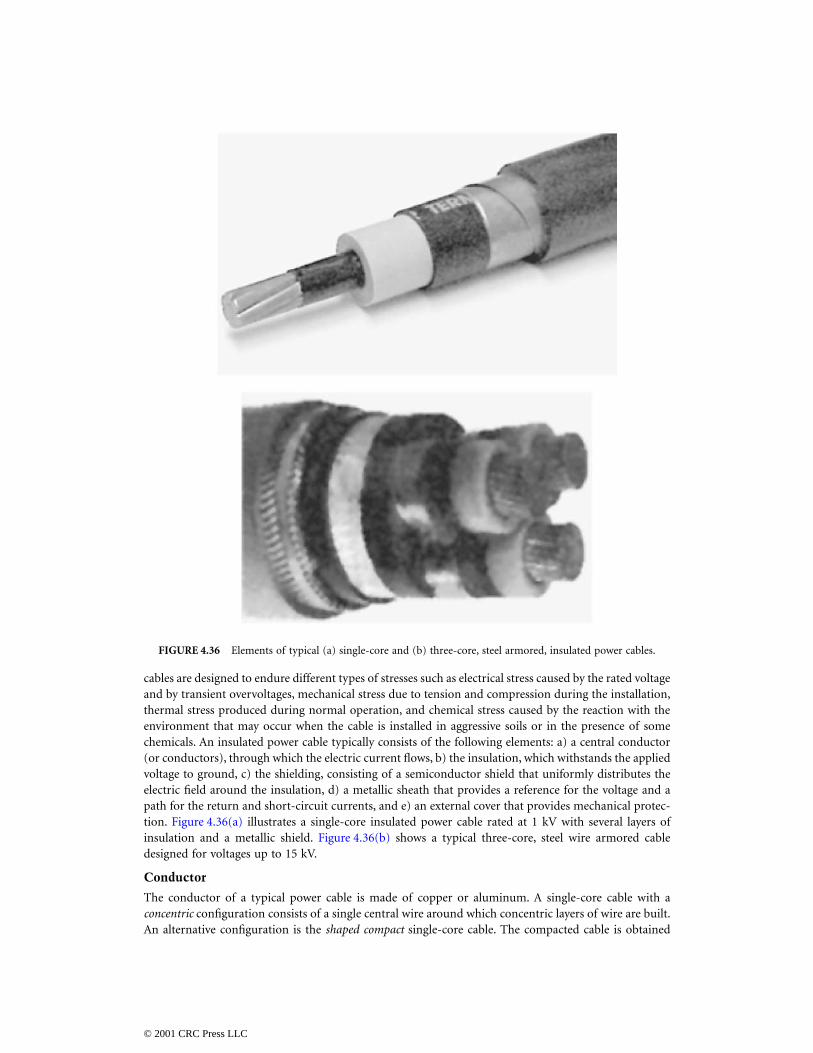
cables are designed to endure different types of stresses such as electrical stress caused by the rated voltageand by transient overvoltages, mechanical stress due to tension and compression during the installation,thermal stress produced during normal operation, and chemical stress caused by the reaction with theenvironment that may occur when the cable is installed in aggressive soils or in the presence of somechemicals. An insulated power cable typically consists of the following elements: a) a central conductor(or conductors), through which the electric current flows, b) the insulation, which withstands the appliedvoltage to ground, c) the shielding, consisting of a semiconductor shield that uniformly distributes theelectric field around the insulation, d) a metallic sheath that provides a reference for the voltage and apath for the return and short-circuit currents, and e) an external cover that provides mechanical protec-tion. Figure 4.36(a) illustrates a single-core insulated power cable rated at 1 kV with several layers ofinsulation and a metallic shield. Figure 4.36(b) shows a typical three-core, steel wire armored cabledesigned for voltages up to 15 kV.

Conductor

The conductor of a typical power cable is made of copper or aluminum. A single-core cable with aconcentric configuration consists of a single central wire around which concentric layers of wire are built.An alternative configuration is the shaped compact single-core cable. The compacted cable is obtained

FIGURE 4.36 Elements of typical (a) single-core and (b) three-core, steel armored, insulated power cables.


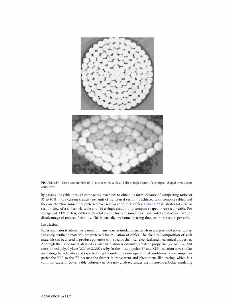
by passing the cable through compacting machines to obtain its form. Because of compacting ratios of85 to 90%, more current capacity per unit of transversal section is achieved with compact cables, andthey are therefore sometimes preferred over regular concentric cables. Figure 4.37 illustrates (a) a cross-section view of a concentric cable and (b) a single section of a compact-shaped three-sector cable. Forvoltages of 1 kV or less, cables with solid conductors are sometimes used. Solid conductors have thedisadvantage of reduced flexibility. This is partially overcome by using three or more sectors per core.

Insulation

Paper and natural rubbers were used for many years as insulating materials in underground power cables.Presently, synthetic materials are preferred for insulation of cables. The chemical composition of suchmaterials can be altered to produce polymers with specific chemical, electrical, and mechanical properties.Although the list of materials used as cable insulation is extensive, ethylene propylene (EP or EPR) andcross-linked polyethylene (XLP or XLPE) are by far the most popular. EP and XLP insulation have similarinsulating characteristics and expected long life under the same operational conditions. Some companiesprefer the XLP to the EP because the former is transparent and phenomena like treeing, which is acommon cause of power cable failures, can be easily analyzed under the microscope. Other insulating

FIGURE 4.37 Cross-section view of (a) a concentric cable and (b) a single sector of a compact-shaped three-sectorconductor.


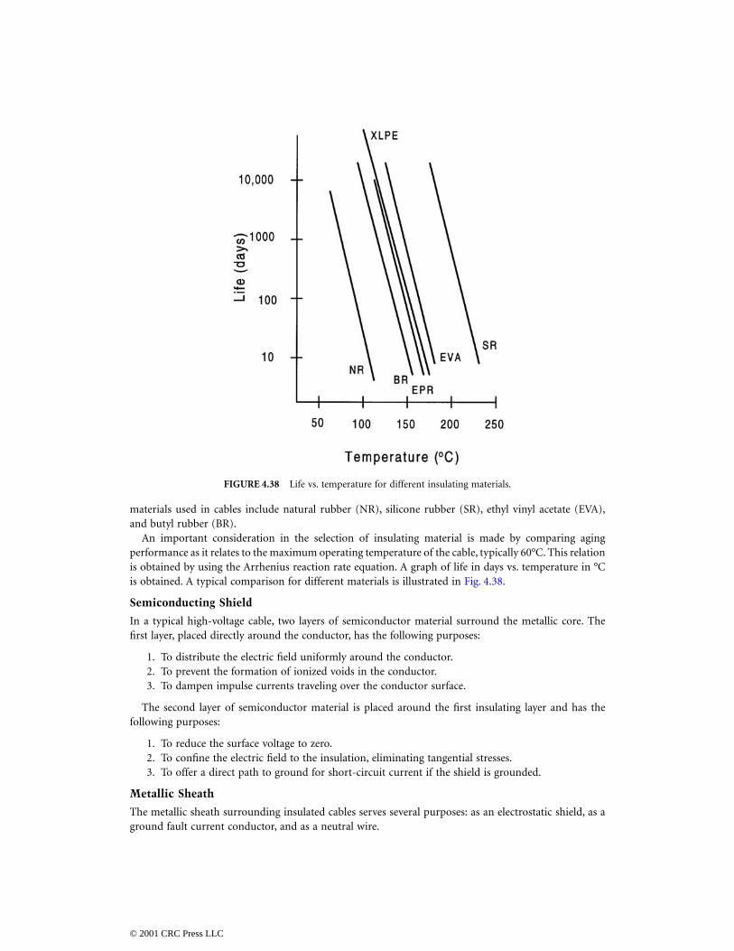
materials used in cables include natural rubber (NR), silicone rubber (SR), ethyl vinyl acetate (EVA),and butyl rubber (BR).

An important consideration in the selection of insulating material is made by comparing agingperformance as it relates to the maximum operating temperature of the cable, typically 60°C. This relationis obtained by using the Arrhenius reaction rate equation. A graph of life in days vs. temperature in °Cis obtained. A typical comparison for different materials is illustrated in Fig. 4.38.

Semiconducting Shield

In a typical high-voltage cable, two layers of semiconductor material surround the metallic core. Thefirst layer, placed directly around the conductor, has the following purposes:

1. To distribute the electric field uniformly around the conductor.2. To prevent the formation of ionized voids in the conductor.3. To dampen impulse currents traveling over the conductor surface.

The second layer of semiconductor material is placed around the first insulating layer and has thefollowing purposes:

1. To reduce the surface voltage to zero.2. To confine the electric field to the insulation, eliminating tangential stresses.3. To offer a direct path to ground for short-circuit current if the shield is grounded.

Metallic Sheath

The metallic sheath surrounding insulated cables serves several purposes: as an electrostatic shield, as aground fault current conductor, and as a neutral wire.

FIGURE 4.38 Life vs. temperature for different insulating materials.


1. The metallic sheath designed for electrostatic purpose should be made of non-magnetic tape ornon-magnetic wires. Copper is usually used for these sheaths.

2. When properly grounded, this sheath provides a path for short-circuit current.3. With appropriate dimensions, the metallic sheath can be used as a system neutral, as in residential

distribution cables where single-phase transformers are common. When single-core cables areused in three-phase systems, the grounded sheath provides a path for unbalanced currents.

When high-voltage underground cables require some type of moisture insulating barrier, a metallicpipe surrounds the current-carrying cable. The materials most commonly used as moisture barriers arelead and aluminum. The electric currents carried by the high-voltage cable will induce a voltage in themetallic shield that surrounds the conductor, and in the shields of other surrounding cables. Theseinduced voltages, in turn, will generate an induced current flow with its associated heat losses. In thecase of steel shields, the losses will include magnetization and hysteresis losses.

External Layer

The purpose of the external layer in insulated power cables is to provide mechanical protection againstthe environment during the installation and operation of the power cable. Currently, materials commonlyused as the external layer for extruded power cables include PVC and polyethylene of low and highdensity. These materials are used for their ability to withstand the cable operating temperature, theirresistance to excessive degradation when in contact with some chemicals typical of some operatingenvironments, and their excellent mechanical properties for undergoing stresses during transportation,or compression and tension during installation and operation.

Overview of Electric Parameters of Underground Power Cables

Cable Electrical Resistance

The cable operation parameters determine the cable behavior under emergency and normal operatingconditions. The cable impedance, (R + jXL), is useful for calculating regulation and losses under normalconditions and short-circuit current magnitude under short-circuit fault conditions. Alterations inparameters due to temperature and length variations include the change of resistance. In order to simplifythe selection of a power cable for a given application, the maximum cable operating temperature isdetermined based on engineering calculations and laboratory tests. In the case of single wires, which arestranded together following a helical path to form a cable, a factor must be added to account for theextra length. In multi-core cables, the extra length due to the layout of the individual cores must also beaccounted for. To simplify the calculation of electrical parameters, graphs of conductor size vs. resistancein ohm/kilometer can be developed and are provided by the manufacturer. Typically, manufacturersprovide AC and DC resistance values which are temperature dependent. In general, the DC resistance isgiven by:

(4.4)

where

Rtc = conductor resistance at temperature tc°C (in ohms)R20 = conductor resistance at temperature 20°C (in ohms)α20 = temperature coefficient of resistance of conductor material at 20°Ctc = conductor temperature (in °C)

The AC resistance of cables is important because it affects the current-carrying capacity. The ACresistance of cables is affected mainly by skin effect and proximity effect. The analysis of these effects iscomplicated and graphs and tables provided by the cable manufacturer should be used to simplify any

R R tt cc= + −( )[ ]20 201 20α


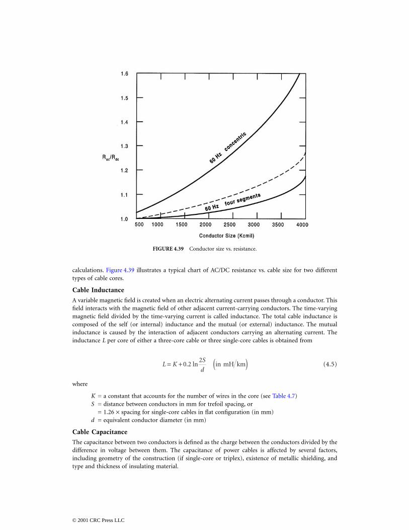
calculations. Figure 4.39 illustrates a typical chart of AC/DC resistance vs. cable size for two differenttypes of cable cores.

Cable Inductance

A variable magnetic field is created when an electric alternating current passes through a conductor. Thisfield interacts with the magnetic field of other adjacent current-carrying conductors. The time-varyingmagnetic field divided by the time-varying current is called inductance. The total cable inductance iscomposed of the self (or internal) inductance and the mutual (or external) inductance. The mutualinductance is caused by the interaction of adjacent conductors carrying an alternating current. Theinductance L per core of either a three-core cable or three single-core cables is obtained from

(4.5)

where

K = a constant that accounts for the number of wires in the core (see Table 4.7)S = distance between conductors in mm for trefoil spacing, or

= 1.26 × spacing for single-core cables in flat configuration (in mm)d = equivalent conductor diameter (in mm)

Cable Capacitance

The capacitance between two conductors is defined as the charge between the conductors divided by thedifference in voltage between them. The capacitance of power cables is affected by several factors,including geometry of the construction (if single-core or triplex), existence of metallic shielding, andtype and thickness of insulating material.

FIGURE 4.39 Conductor size vs. resistance.

L KS

d= + ( )0 2

2. ln in mH km


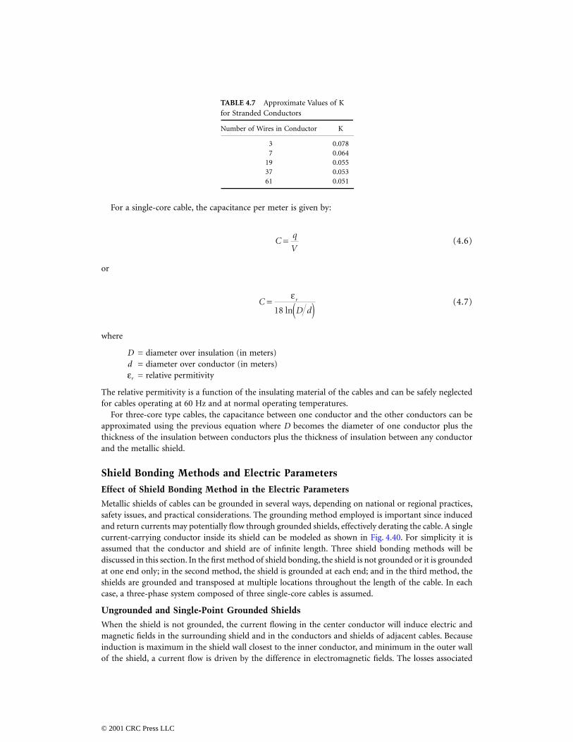
For a single-core cable, the capacitance per meter is given by:

(4.6)

or

(4.7)

where

D = diameter over insulation (in meters)d = diameter over conductor (in meters)εr = relative permitivity

The relative permitivity is a function of the insulating material of the cables and can be safely neglectedfor cables operating at 60 Hz and at normal operating temperatures.

For three-core type cables, the capacitance between one conductor and the other conductors can beapproximated using the previous equation where D becomes the diameter of one conductor plus thethickness of the insulation between conductors plus the thickness of insulation between any conductorand the metallic shield.

Shield Bonding Methods and Electric Parameters

Effect of Shield Bonding Method in the Electric Parameters

Metallic shields of cables can be grounded in several ways, depending on national or regional practices,safety issues, and practical considerations. The grounding method employed is important since inducedand return currents may potentially flow through grounded shields, effectively derating the cable. A singlecurrent-carrying conductor inside its shield can be modeled as shown in Fig. 4.40. For simplicity it isassumed that the conductor and shield are of infinite length. Three shield bonding methods will bediscussed in this section. In the first method of shield bonding, the shield is not grounded or it is groundedat one end only; in the second method, the shield is grounded at each end; and in the third method, theshields are grounded and transposed at multiple locations throughout the length of the cable. In eachcase, a three-phase system composed of three single-core cables is assumed.

Ungrounded and Single-Point Grounded Shields

When the shield is not grounded, the current flowing in the center conductor will induce electric andmagnetic fields in the surrounding shield and in the conductors and shields of adjacent cables. Becauseinduction is maximum in the shield wall closest to the inner conductor, and minimum in the outer wallof the shield, a current flow is driven by the difference in electromagnetic fields. The losses associated

TABLE 4.7 Approximate Values of K for Stranded Conductors

Number of Wires in Conductor K

3 0.0787 0.064

19 0.05537 0.05361 0.051

Cq

V=

CD dr= ( )

ε18 ln


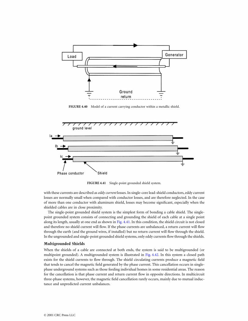
with these currents are described as eddy current losses. In single-core lead-shield conductors, eddy currentlosses are normally small when compared with conductor losses, and are therefore neglected. In the caseof more than one conductor with aluminum shield, losses may become significant, especially when theshielded cables are in close proximity.

The single-point grounded shield system is the simplest form of bonding a cable shield. The single-point grounded system consists of connecting and grounding the shield of each cable at a single pointalong its length, usually at one end as shown in Fig. 4.41. In this condition, the shield circuit is not closedand therefore no shield current will flow. If the phase currents are unbalanced, a return current will flowthrough the earth (and the ground wires, if installed) but no return current will flow through the shield.In the ungrounded and single-point grounded shield systems, only eddy currents flow through the shields.

Multigrounded Shields

When the shields of a cable are connected at both ends, the system is said to be multigrounded (ormultipoint grounded). A multigrounded system is illustrated in Fig. 4.42. In this system a closed pathexists for the shield currents to flow through. The shield circulating currents produce a magnetic fieldthat tends to cancel the magnetic field generated by the phase current. This cancellation occurs in single-phase underground systems such as those feeding individual homes in some residential areas. The reasonfor the cancellation is that phase current and return current flow in opposite directions. In multicircuitthree-phase systems, however, the magnetic field cancellation rarely occurs, mainly due to mutual induc-tance and unpredicted current unbalances.

FIGURE 4.40 Model of a current carrying conductor within a metallic shield.

FIGURE 4.41 Single-point grounded shield system.


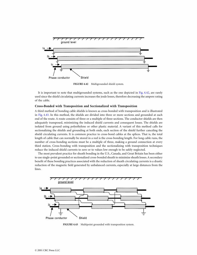
It is important to note that multigrounded systems, such as the one depicted in Fig. 4.42, are rarelyused since the shield circulating currents increases the joule losses, therefore decreasing the ampere ratingof the cable.

Cross-Bonded with Transposition and Sectionalized with Transposition

A third method of bonding cable shields is known as cross-bonded with transposition and is illustratedin Fig. 4.43. In this method, the shields are divided into three or more sections and grounded at eachend of the route. A route consists of three or a multiple of three sections. The conductor shields are thenadequately transposed, minimizing the induced shield currents and consequent losses. The shields areisolated from ground using polyethylene or other plastic material. A variant of this method calls forsectionalizing the shields and grounding at both ends, each section of the shield further canceling theshield circulating currents. It is common practice to cross-bond cables at the splices. That is, the totallength of cable that can normally be stored in a reel is the cross-bonding length. For long cable runs, thenumber of cross-bonding sections must be a multiple of three, making a ground connection at everythird station. Cross-bonding with transposition and the sectionalizing with transposition techniquesreduce the induced shield currents to zero or to values low enough to be safely neglected.

The most prevalent practice for sheath bonding in the U.S., Canada, and Great Britain has been eitherto use single-point grounded or sectionalized cross-bonded sheath to minimize sheath losses. A secondarybenefit of these bonding practices associated with the reduction of sheath circulating currents is a drasticreduction of the magnetic field generated by unbalanced currents, especially at large distances from thelines.

FIGURE 4.42 Multigrounded shield system.

FIGURE 4.43 Multipoint grounded with transposition system.


Calculation of Losses

When the sheath is grounded or bonded to earth at more than one point, current flows through thesheath due to the emf induced in it by the alternating current in the central conductor. The mechanismof induction is the same as the mechanism of induction in a transformer. The induced voltage in thesheath of such conductor is:

(4.8)

where

I

= conductor current in amperes and

(4.9)

where the mutual inductance between conductors and sheath is:

(4.10)

The impedance of the sheath is given by:

(4.11)

where R

s

is the sheath resistance.The sheath current is therefore:

(4.12)

or

(4.13)

Finally, the sheath current losses per phase is given by:

(4.14)

The calculations described above assume that voltage induction by nearby conductors and nearbysheaths is negligible.

Underground Layout and Construction

Residential Distribution Layout

In general, the design of underground distribution systems feeding residential areas is similar to overheaddistribution systems. As in overhead systems, a primary main is installed from which distributiontransformers supply consumers at a lower voltage (120–240 V). There are two widely used circuit

E I Xs m=

X fMm = π ( )−2 10 3 in ohms km

MS

de

m

= ( )0 22

. log in mH km

Z R Xs s m= + ( )2 2 in ohms km

IE

R Xs

s

s m

=+2 2

IIX

R Xs

m

s m

=+2 2

I RI X R

R Xs s

m s

s m

22 2

2 2=

+( ) in watts km


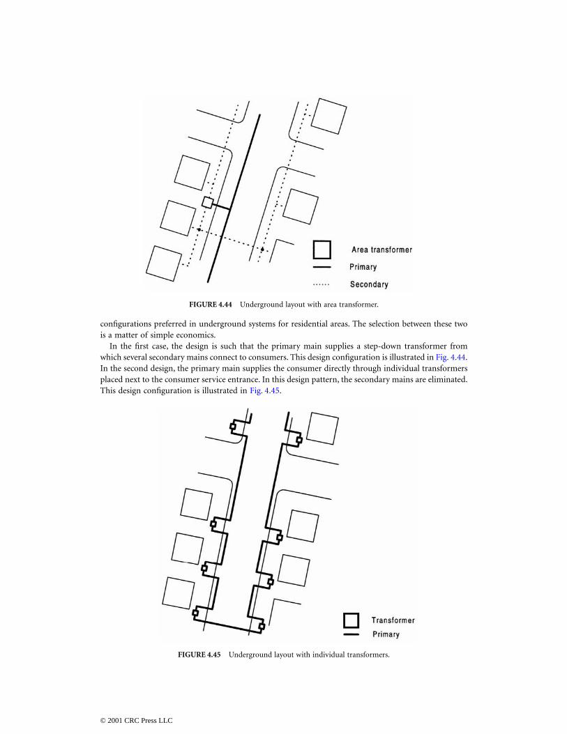
configurations preferred in underground systems for residential areas. The selection between these twois a matter of simple economics.

In the first case, the design is such that the primary main supplies a step-down transformer fromwhich several secondary mains connect to consumers. This design configuration is illustrated in Fig. 4.44.In the second design, the primary main supplies the consumer directly through individual transformersplaced next to the consumer service entrance. In this design pattern, the secondary mains are eliminated.This design configuration is illustrated in Fig. 4.45.

FIGURE 4.44

Underground layout with area transformer.

FIGURE 4.45

Underground layout with individual transformers.


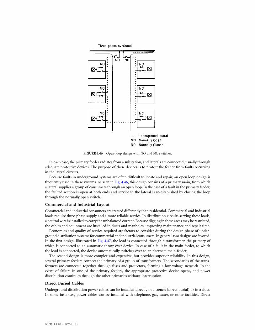
In each case, the primary feeder radiates from a substation, and laterals are connected, usually throughadequate protective devices. The purpose of these devices is to protect the feeder from faults occurringin the lateral circuits.

Because faults in underground systems are often difficult to locate and repair, an open loop design isfrequently used in these systems. As seen in Fig. 4.46, this design consists of a primary main, from whicha lateral supplies a group of consumers through an open loop. In the case of a fault in the primary feeder,the faulted section is open at both ends and service to the lateral is re-established by closing the loopthrough the normally open switch.

Commercial and Industrial Layout

Commercial and industrial consumers are treated differently than residential. Commercial and industrialloads require three-phase supply and a more reliable service. In distribution circuits serving these loads,a neutral wire is installed to carry the unbalanced current. Because digging in these areas may be restricted,the cables and equipment are installed in ducts and manholes, improving maintenance and repair time.

Economics and quality of service required are factors to consider during the design phase of under-ground distribution systems for commercial and industrial consumers. In general, two designs are favored.In the first design, illustrated in Fig. 4.47, the load is connected through a transformer, the primary ofwhich is connected to an automatic throw-over device. In case of a fault in the main feeder, to whichthe load is connected, the device automatically switches over to an alternate main feeder.

The second design is more complex and expensive, but provides superior reliability. In this design,several primary feeders connect the primary of a group of transformers. The secondaries of the trans-formers are connected together through fuses and protectors, forming a low-voltage network. In theevent of failure in one of the primary feeders, the appropriate protective device opens, and powerdistribution continues through the other primaries without interruption.

Direct Buried Cables

Underground distribution power cables can be installed directly in a trench (direct burial) or in a duct.In some instances, power cables can be installed with telephone, gas, water, or other facilities. Direct

FIGURE 4.46

Open-loop design with NO and NC switches.


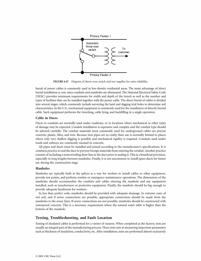
burial of power cables is commonly used in low-density residential areas. The main advantage of directburial installation is cost, since conduits and manholes are eliminated. The National Electrical Safety Code(NESC) provides minimum requirements for width and depth of the trench as well as the number andtypes of facilities that can be installed together with the power cable. The direct burial of cables is dividedinto several stages, which commonly include surveying the land and digging trial holes to determine soilcharacteristics. In the U.S., mechanized equipment is commonly used for the installation of directly buriedcable. Such equipment performs the trenching, cable lying, and backfilling in a single operation.

Cable in Ducts

Ducts or conduits are normally used under roadways, or in locations where mechanical or other typesof damage may be expected. Conduit installation is expensive and complex and the conduit type shouldbe selected carefully. The conduit materials most commonly used for underground cables are precastconcrete, plastic, fiber, and iron. Because iron pipes are so costly, their use is normally limited to placeswhere only very shallow digging is possible and mechanical rigidity is required. Conduits used underroads and railways are commonly encased in concrete.

All pipes and ducts must be installed and joined according to the manufacturer’s specifications. It iscommon practice to seal the duct to prevent foreign materials from entering the conduit. Another practiceconsists of including a noncorroding draw line in the duct prior to sealing it. This is a beneficial provision,especially in long lengths between manholes. Finally, it is not uncommon to install spare ducts for futureuse during the construction stage.

Manholes

Manholes are typically built at the splices as a way for workers to install cables or other equipment,provide test points, and perform routine or emergency maintenance operations. The dimensions of themanholes should accommodate the conduits and cables entering the manhole and any equipmentinstalled, such as transformers or protective equipment. Finally, the manhole should be big enough toprovide adequate headroom for workers.

In less than perfect soils, manholes should be provided with adequate drainage. In extreme cases ofwet soil, and if sewer connections are possible, appropriate connections should be made from themanholes to the sewer lines. If sewer connections are not possible, manholes should be constructed withwaterproof concrete. This is a necessary requirement where the natural water table is higher than thebottom of the manhole.

Testing, Troubleshooting, and Fault Location

Testing of insulated cables is performed for a variety of reasons. When completed at the factory, tests areusually an integral part of the manufacturing process. These tests aim at measuring important parameterssuch as thickness of insulation, conductivity, etc. After installation, tests are performed almost exclusively

FIGURE 4.47

Diagram of throw-over switch and two supplies for extra reliability.


to detect the location of failures. This section presents an overview of some commonly performed pre-and post-installation tests.

Four types of tests are performed on cables:

1. Routine tests performed on every cable to ensure compliance with specifications and the integrityof every cable.

2. Sample tests performed periodically on cable samples to ensure manufacturing consistency.3. Experimental tests performed to determine characteristics of newly developed materials.4. Site tests performed after installation in the field.

Tests 1 through 3 provide insight into cable dimensions, insulation resistance and capacitance. Inaddition, high voltage, impulse voltage, and measurement of partial discharge trials are performed aspart of these tests.

Impulse Test

The purpose of the impulse voltage test is to check the cable under conditions of transient overvoltagesor other temporary high-voltage surges normally associated with switching operations or atmosphericdischarges. Such conditions are often encountered during the regular operation of a cable. During atypical impulse voltage test, the cable is first subjected to mechanical stresses typically found in a routineinstallation procedure, such as bending. A set of negative and positive impulses at the withstand levelare applied to the cable which has been heated at the maximum conductor temperature. After the impulsesare applied, the cable may be subjected to a high-voltage test.

High-Voltage Test

High-voltage tests are performed to locate defects in insulated cables. The selection of voltage level isextremely important: if the voltage is too high, it may cause incipient damage of the cable, affectingfuture service life. On the other hand, the breakdown of the insulation under high voltage is also timedependent and therefore a number of voltage/time to breakdown tests are performed. These tests areimportant for developmental purposes but have little use as predictors of service life.

Partial Discharge Test

Gas-filled voids are found in the insulation and at the juncture of dielectric and conductive sheaths of cables.The breakdown of this gas produces a phenomenon known as partial discharge. Partial discharge occurs atthese voids because the breakdown strength of the gas within voids is much less than that of the typicalcable insulation material. In fact, discharges may occur at voltages lower than the operating voltage of thecable. The level of voltage at which partial discharge occurs first is called the discharge inception voltage.

Incidence of Faults and Fault Location

The major causes of faults in underground cables (listed below) are an indication of some of the hazardsto which cables are exposed: accidental contact, aging, faulty installation, lightning, and others. Depend-ing on the location, accidental contact and aging account for more than 50% of all faults. Becauseaccidental contacts with cables often produce only minor damage, there is a time lapse until the cabledeteriorates enough to produce failure and operation of protective equipment. When there is accidentalcontact with cables, failures may occur as a result of prolonged exposure to moisture, loss of dielectricmaterial, corrosion, etc.

An effective location of faults in an underground cable system requires a systematic approach. Typically,the following steps are followed to successfully locate a fault:

1. The existence and type of fault is first determined. This requires the determination of damage tothe shield and or changes in continuity of the conductor.

2. Once the existence of the fault is assured, it is necessary to diagnose the cause of the fault. Thiscan be determined in several ways, including ruling out faulty operation of protective equipment.A Megger may be used to check continuity.


3. In the case of intermittent faults, preconditioning of the cable may be required to produce a“stable” fault. This step may or may not be required, depending on the type of equipment availablefor fault location. The most common preconditioning technique used consists of allowing currentto pass through the fault to carbonize the insulation.

4. Once a consistent fault is observed, procedures for fault prelocation are followed. This is knownas pinpointing the fault location. This step assures that the location and repair of a faultedunderground cable will be accomplished in one single excavation. Most modern instruments usedto pinpoint faults are based on traveling waves theory.

References

Ametani, A., A general formulation of impedance and admittance of cables,

IEEE Trans. PAS-99

, 3,902-910, May/June 1980.

Densley, R. J., An investigation into the growth of electrical trees in XLPE cable insulation,

IEEE Trans.EI-14

, 148-158, June 1979.Gale, P. F., Cable fault location by impulse current method,

Proc. IEEE 122

, 403-408, April 1975.Graneau, P.,

Underground Power Transmission: The Science, Technology, and Economics of High VoltageCables

, John Wiley & Sons, New York, 1979.IEEE Guide for the Application of Sheath-Bonding Methods for Single-Conductor Cable and the Calcu-

lation of Induced Voltages and Currents in Cable Sheaths.

ANSI/IEEE Std. 575-1988

.Kalsi, S. S. and Minnich, S. H., Calculation of circulating current losses in cable conductors,

IEEE Trans.PAS-99

, March/April, 1980.Kojima, K. et al., Development and commercial use of 275 kV XLPE power cable,

IEEE Trans. PAS-100

,1, 203-210.

McAllister, D.,

Electric Cables Handbook

, Granada Publishing Ltd., Great Britain, 1982.Milne, A. G. and Mochlinski, K., Characteristics of soil affecting cable ratings,

Proc. IEEE 111

(5), 1964.Pansini, A.,

Guide to Electrical Power Distribution Systems

, Pennwell Books, Tulsa, OK, 1996.Transmission cable magnetic field research,

EPRI EL-6759-D, Project 7898-21, Final Report

, April 1990.

4.6 Transmission Line Parameters

Manuel Reta-Hernández

The power transmission line is one of the major components of an electric power system. Its majorfunction is to transport electric energy, with minimal losses, from the power sources to the load centers,usually separated by long distances. The three basic electrical parameters of a transmission line are:

1. Series resistance2. Series inductance3. Shunt capacitance

Once evaluated, the parameters are used to model the line and to perform design calculations. Thearrangement of the parameters (equivalent circuit) representing the line depends upon the length of theline.

Equivalent Circuit

A transmission line is defined as a short-length line if its length is less than 80 km (50 mi). In this case,the capacitive effect is negligible and only the resistance and inductive reactance are considered. Assumingbalanced conditions, the line can be represented by the equivalent circuit of a single phase with resistance

R

,and inductive reactance

X

L

in series, as shown in Fig. 4.48.


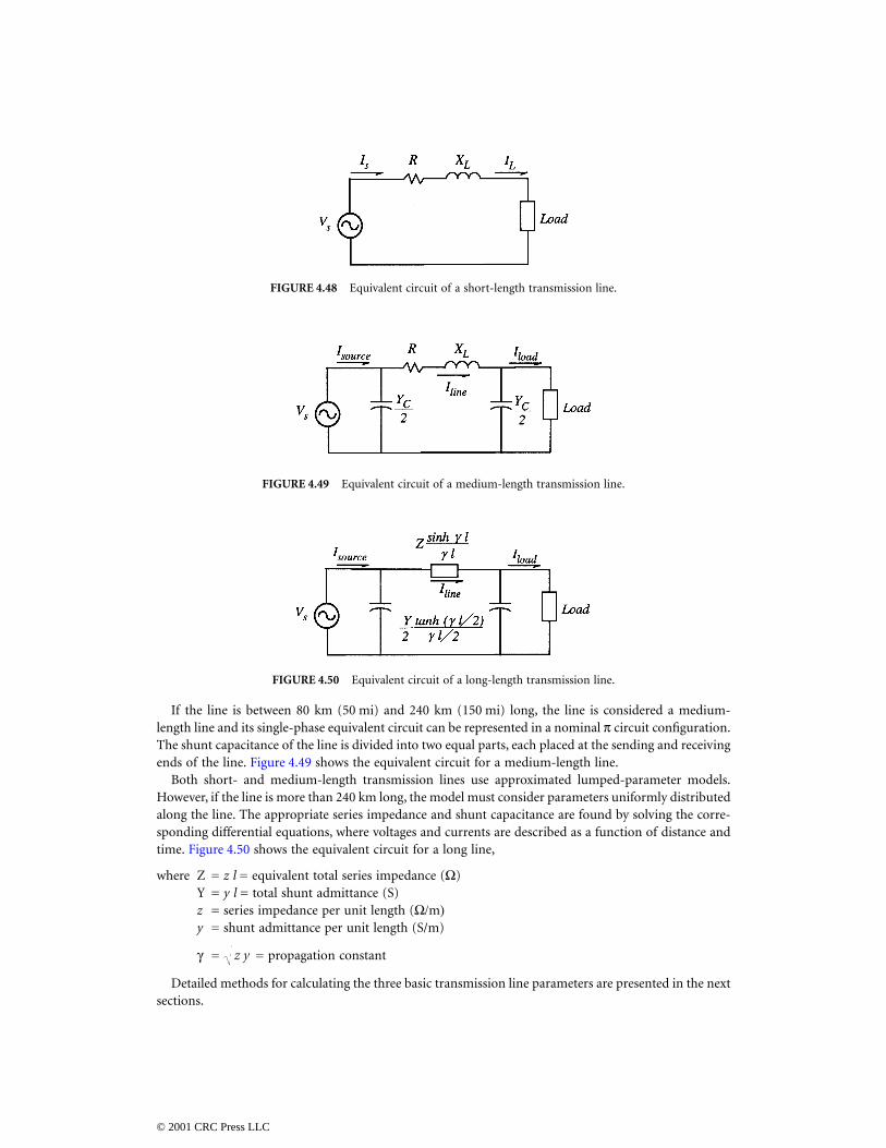
If the line is between 80 km (50 mi) and 240 km (150 mi) long, the line is considered a medium-length line and its single-phase equivalent circuit can be represented in a nominal

π

circuit configuration.The shunt capacitance of the line is divided into two equal parts, each placed at the sending and receivingends of the line. Figure 4.49 shows the equivalent circuit for a medium-length line.

Both short- and medium-length transmission lines use approximated lumped-parameter models.However, if the line is more than 240 km long, the model must consider parameters uniformly distributedalong the line. The appropriate series impedance and shunt capacitance are found by solving the corre-sponding differential equations, where voltages and currents are described as a function of distance andtime. Figure 4.50 shows the equivalent circuit for a long line,

where Z =

z l

= equivalent total series impedance (

Ω

)Y =

y l

= total shunt admittance (S)

z

= series impedance per unit length (

Ω/

m

)

y

= shunt admittance per unit length (S/m)

γ

= = propagation constant

Detailed methods for calculating the three basic transmission line parameters are presented in the nextsections.

FIGURE 4.48

Equivalent circuit of a short-length transmission line.

FIGURE 4.49

Equivalent circuit of a medium-length transmission line.

FIGURE 4.50

Equivalent circuit of a long-length transmission line.

z y


Resistance

The AC resistance of a conductor in a transmission line is based on the calculation of its DC resistance.If DC is flowing along a round cylindrical conductor, the current is uniformly distributed over its cross-section area and the DC resistance is evaluated by:

(4.15)

where

ρ

= conductor resistivity at a given temperature (

Ω

-m)

l

= conductor length (m)

A

= conductor cross-section area (m

2

)

If AC current is flowing, rather than DC current, the conductor effective resistance is higher due tothe skin effect (presented in the next section).

Frequency Effect

The frequency of the AC voltage produces a second effect on the conductor resistance due to thenonuniform distribution of the current. This phenomenon is known as skin effect. As frequency increases,the current tends to go toward the surface of the conductor and the current density decreases at thecenter. Skin effect reduces the effective cross-section area used by the current and thus the effectiveresistance increases. Also, although in small amount, a further resistance increase occurs when othercurrent-carrying conductors are present in the immediate vicinity. A skin correction factor

k

, obtainedby differential equations and Bessel functions, is considered to reevaluate the AC resistance. For 60 Hz,

k

is estimated around 1.02:

(4.16)

Other variations in resistance are caused by:

• temperature

• spiraling of stranded conductors

• bundle conductors arrangement

Temperature Effect

The resistivity of any metal varies linearly over an operating temperature, and therefore the resistance ofany conductor suffers the same variations. As temperature rises, the resistance increases linearly, accordingto the following equation:

(4.17)

where

R

2

= resistance at second temperature

t

2

(°C)

R

1

= resistance at initial temperature

t

1

(°C)

T

= temperature coefficient for the particular material (°C)

Resistivity (

ρ

) and temperature coefficient (

T

) constants depend on the particular conductor material.Table 4.8 lists resistivity and temperature coefficients of some typical conductor materials.

Spiraling and Bundle Conductor Effect

There are two types of transmission line conductors: overhead and underground. Overhead conductors,made of naked metal and suspended on insulators, are preferred over underground conductors becauseof the lower cost and ease of maintenance.

Rl

Adc = [ ]ρ Ω

R R kac ac=

R RT t

T t2 12

1

= ++


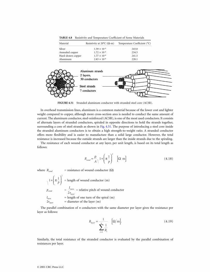
In overhead transmission lines, aluminum is a common material because of the lower cost and lighterweight compared to copper, although more cross-section area is needed to conduct the same amount ofcurrent. The aluminum conductor, steel-reinforced (ACSR), is one of the most used conductors. It consistsof alternate layers of stranded conductors, spiraled in opposite directions to hold the strands together,surrounding a core of steel strands as shown in Fig. 4.51. The purpose of introducing a steel core insidethe stranded aluminum conductors is to obtain a high strength-to-weight ratio. A stranded conductoroffers more flexibility and is easier to manufacture than a solid large conductor. However, the totalresistance is increased because the outside strands are larger than the inside strands due to the spiraling.

The resistance of each wound conductor at any layer, per unit length, is based on its total length asfollows:

(4.18)

where

R

cond

= resistance of wound conductor (

Ω)

= length of wound conductor (m)

p

cond

= = relative pitch of wound conductor

l

turn

= length of one turn of the spiral (m)2

r

layer

= diameter of the layer (m)

The parallel combination of

n

conductors with the same diameter per layer gives the resistance perlayer as follows:

(4.19)

Similarly, the total resistance of the stranded conductor is evaluated by the parallel combination ofresistances per layer.

TABLE 4.8

Resistivity and Temperature Coefficient of Some Materials

Material Resistivity at 20°C (

Ω

-m) Temperature Coefficient (°C)

Silver 1.59

×

10

–8

243.0Annealed copper 1.72

×

10

–8

234.5Hard-drawn copper 1.77

×

10

–8

241.5Aluminum 2.83

×

10

–8

228.1

FIGURE 4.51

Stranded aluminum conductor with stranded steel core (ACSR).

RA pcond = + π

[ ]ρ1

12

Ω m

11

2

+ π

p

I

rturn

layer2

R

R

layer

ii

n= [ ]

=∑

1

1

1

.Ω m


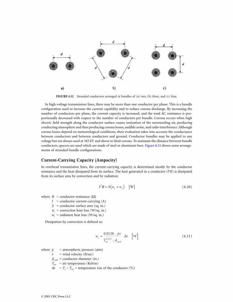
In high-voltage transmission lines, there may be more than one conductor per phase. This is a bundleconfiguration used to increase the current capability and to reduce corona discharge. By increasing thenumber of conductors per phase, the current capacity is increased, and the total AC resistance is pro-portionally decreased with respect to the number of conductors per bundle. Corona occurs when highelectric field strength along the conductor surface causes ionization of the surrounding air, producingconducting atmosphere and thus producing corona losses, audible noise, and radio interference. Althoughcorona losses depend on meteorological conditions, their evaluation takes into account the conductancebetween conductors and between conductors and ground. Conductor bundles may be applied to anyvoltage but are always used at 345 kV and above to limit corona. To maintain the distance between bundleconductors, spacers are used which are made of steel or aluminum bars. Figure 4.52 shows some arrange-ments of stranded bundle configurations.

Current-Carrying Capacity (Ampacity)

In overhead transmission lines, the current-carrying capacity is determined mostly by the conductorresistance and the heat dissipated from its surface. The heat generated in a conductor (

I

2

R

) is dissipatedfrom its surface area by convection and by radiation:

(4.20)

where

R =

conductor resistance (

Ω)I = conductor current-carrying (A)S = conductor surface area (sq. in.)wc = convection heat loss (W/sq. in.)wr = radiation heat loss (W/sq. in.)

Dissipation by convection is defined as:

(4.21)

where p = atmospheric pressure (atm)v = wind velocity (ft/sec)dcond = conductor diameter (in.)Tair = air temperature (Kelvin)∆t = Tc – Tair = temperature rise of the conductor (°C)

FIGURE 4.52 Stranded conductors arranged in bundles of (a) two, (b) three, and (c) four.

I R S w wc r2 = +( ) [ ] W

wpv

T dtc

air cond

= [ ]0 01280 123

.

.∆ W


Dissipation by radiation is obtained from the Stefan-Boltzmann law and is defined as:

(4.22)

where wr = radiation heat loss (W/sq. in.)E = emissivity constant (1 for the absolute black body and 0.5 for oxidized copper)Tc = conductor temperature (°C)Tair = ambient temperature (°C)

Substituting Eqs. (4.21) and (4.22) in (4.20) we can obtain the conductor ampacity at given temperatures.

(4.23)

(4.24)

Some approximated current-carrying capacity values for overhead aluminum and aluminum reinforcedconductors are presented in the section “Characteristics of Overhead Conductors.”

Inductance and Inductive Reactance

The magnetic flux generated by the current in transmission line conductors produces a total inductancewhose magnitude depends on the line configuration. To determine the inductance of the line, it isnecessary to calculate, as in any magnetic circuit with permeability µ:

1. the magnetic field intensity H,2. the magnetic field density B, and3. the flux linkage λ.

Inductance of a Solid, Round, Infinitely Long Conductor

Consider a long, solid, cylindrical conductor with radius r, carrying current I as shown in Fig. 4.53. Ifthe conductor is a nonmagnetic material, and the current is assumed to be uniformly distributed (noskin effect), then the generated internal and external magnetic field lines are concentric circles aroundthe conductor with direction defined by the right-hand rule.

Internal Inductance

To obtain the internal inductance, a magnetic field at radius x inside the conductor is chosen as shownin Fig. 4.54.

The fraction of the current Ix enclosed in the area of the circle is determined by:

(4.25)

Ampere’s law determines the magnetic field intensity Hx constant at any point along the circle contour:

w ET T

rc air=

−

[ ]36 81000 1000

4 4

. W sq. in.

Iw w S

R

c r=+( ) [ ] A

IS

R

t pv

T dE

T T

air cond

c air=

+ −

[ ]

∆ 0 012836 8

10000 123

4 4

4

..

.A

Ix

rIx = π

π [ ]2

2 .A


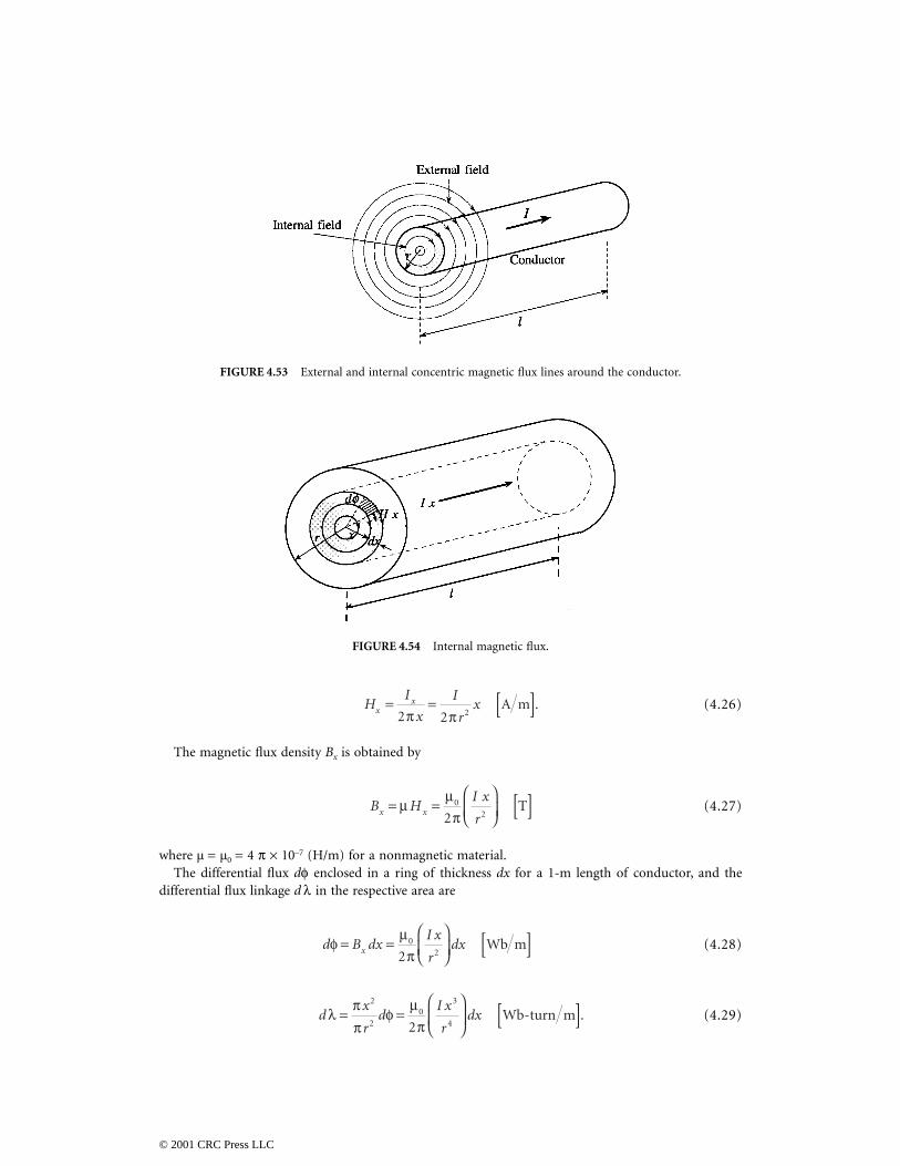
(4.26)

The magnetic flux density Bx is obtained by

(4.27)

where µ = µ0 = 4 π × 10–7 (H/m) for a nonmagnetic material.The differential flux dφ enclosed in a ring of thickness dx for a 1-m length of conductor, and the

differential flux linkage d λ in the respective area are

(4.28)

(4.29)

FIGURE 4.53 External and internal concentric magnetic flux lines around the conductor.

FIGURE 4.54 Internal magnetic flux.

HI

x

I

rxx

x=π

=π [ ]

2 2 2 .A m

B HI x

rx x= µ = µ

π

[ ]0

22 T

d B dxI x

rdxxφ = = µ

π

[ ]0

22 Wb m

dx

rd

I x

rdxλ φ= π

π= µ

π

[ ]

2

20

3

42 .Wb-turn m


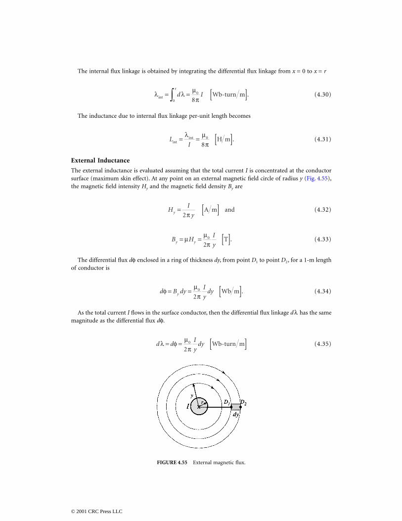
The internal flux linkage is obtained by integrating the differential flux linkage from x = 0 to x = r

(4.30)

The inductance due to internal flux linkage per-unit length becomes

(4.31)

External Inductance

The external inductance is evaluated assuming that the total current I is concentrated at the conductorsurface (maximum skin effect). At any point on an external magnetic field circle of radius y (Fig. 4.55),the magnetic field intensity Hy and the magnetic field density By are

(4.32)

(4.33)

The differential flux dφ enclosed in a ring of thickness dy, from point D1 to point D2, for a 1-m lengthof conductor is

(4.34)

As the total current I flows in the surface conductor, then the differential flux linkage dλ has the samemagnitude as the differential flux dφ.

(4.35)

FIGURE 4.55 External magnetic flux.

λ λint

r

Wb-turn m= = µπ [ ]∫ d I

0

0

8 .

LIintint .= = µ

π [ ]λ 0

8H m

HI

yy =π [ ]

2 A m and

B HI

yy y= µ = µπ [ ]0

2 .T

d B dyI

ydyyφ = = µ

π [ ]0

2 .Wb m

d dI

ydyλ φ= = µ

π [ ]0

2 Wb-turn m


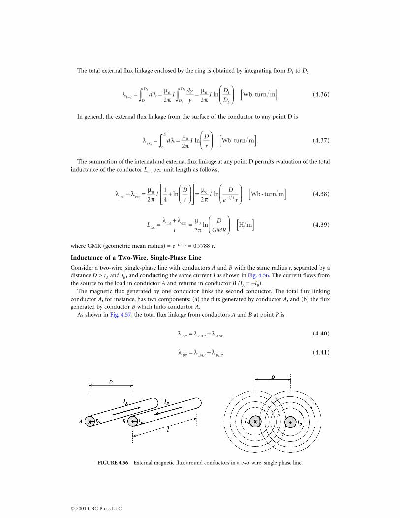
The total external flux linkage enclosed by the ring is obtained by integrating from D1 to D2

(4.36)

In general, the external flux linkage from the surface of the conductor to any point D is

(4.37)

The summation of the internal and external flux linkage at any point D permits evaluation of the totalinductance of the conductor Ltot per-unit length as follows,

(4.38)

(4.39)

where GMR (geometric mean radius) = e –1/4 r = 0.7788 r.

Inductance of a Two-Wire, Single-Phase Line

Consider a two-wire, single-phase line with conductors A and B with the same radius r, separated by adistance D > rA and rB , and conducting the same current I as shown in Fig. 4.56. The current flows fromthe source to the load in conductor A and returns in conductor B (IA = –IB).

The magnetic flux generated by one conductor links the second conductor. The total flux linkingconductor A, for instance, has two components: (a) the flux generated by conductor A, and (b) the fluxgenerated by conductor B which links conductor A.

As shown in Fig. 4.57, the total flux linkage from conductors A and B at point P is

(4.40)

(4.41)

FIGURE 4.56 External magnetic flux around conductors in a two-wire, single-phase line.

λ λ1 20 0 1

21

2

1

2

2 2− = = µπ

= µπ

[ ]∫ ∫d I

dy

yI

D

DD

D

D

D

ln .Wb-turn m

λ λext Wb-turn m= = µπ

[ ]∫ d ID

rr

D0

2ln .

λ λintl ext Wb-turn m+ = µπ

+

= µπ

[ ]−

0 01 42

1

4 2I

D

rI

D

e rln ln

LI

D

GMRtotext H m= + = µ

π

[ ]λ λint ln 0

2

λ λ λAP AAP ABP= +

λ λ λBP BAP BBP= +


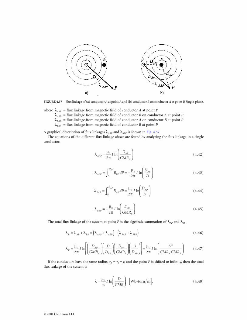
where λAAP = flux linkage from magnetic field of conductor A at point PλABP = flux linkage from magnetic field of conductor B on conductor A at point PλBAP = flux linkage from magnetic field of conductor A on conductor B at point PλBBP = flux linkage from magnetic field of conductor B at point P

A graphical description of flux linkages λAAP and λABP is shown in Fig. 4.57.The equations of the different flux linkage above are found by analyzing the flux linkage in a single

conductor.

(4.42)

(4.43)

(4.44)

(4.45)

The total flux linkage of the system at point P is the algebraic summation of λAP and λBP

(4.46)

(4.47)

If the conductors have the same radius, rA = rB = r, and the point P is shifted to infinity, then the totalflux leakage of the system is

(4.48)

FIGURE 4.57 Flux linkage of (a) conductor A at point P, and (b) conductor B on conductor A at point P. Single-phase.

λAAPAP

A

ID

GMR= µ

π

0

2ln

λABP BPD

DBPB dP I

D

D

BP

= = − µπ

∫ 0

2ln

λBAP APD

DAPB dP I

D

D

AP

= = µπ

∫ 0

2ln

λBBPBP

B

ID

GMR= − µ

π

0

2ln

λ λ λ λ λ λ λP AP BP AAP ABP BAP BBP= + = +( ) − +( )

λPAP

A BP

BP

B AP A B

ID

GMR

D

D

D

GMR

D

DI

D

GMR GMR= µ

π

= µπ

0 0

2

2 2ln ln

λ = µπ

[ ]0 ID

GMRln ,Wb-turn m


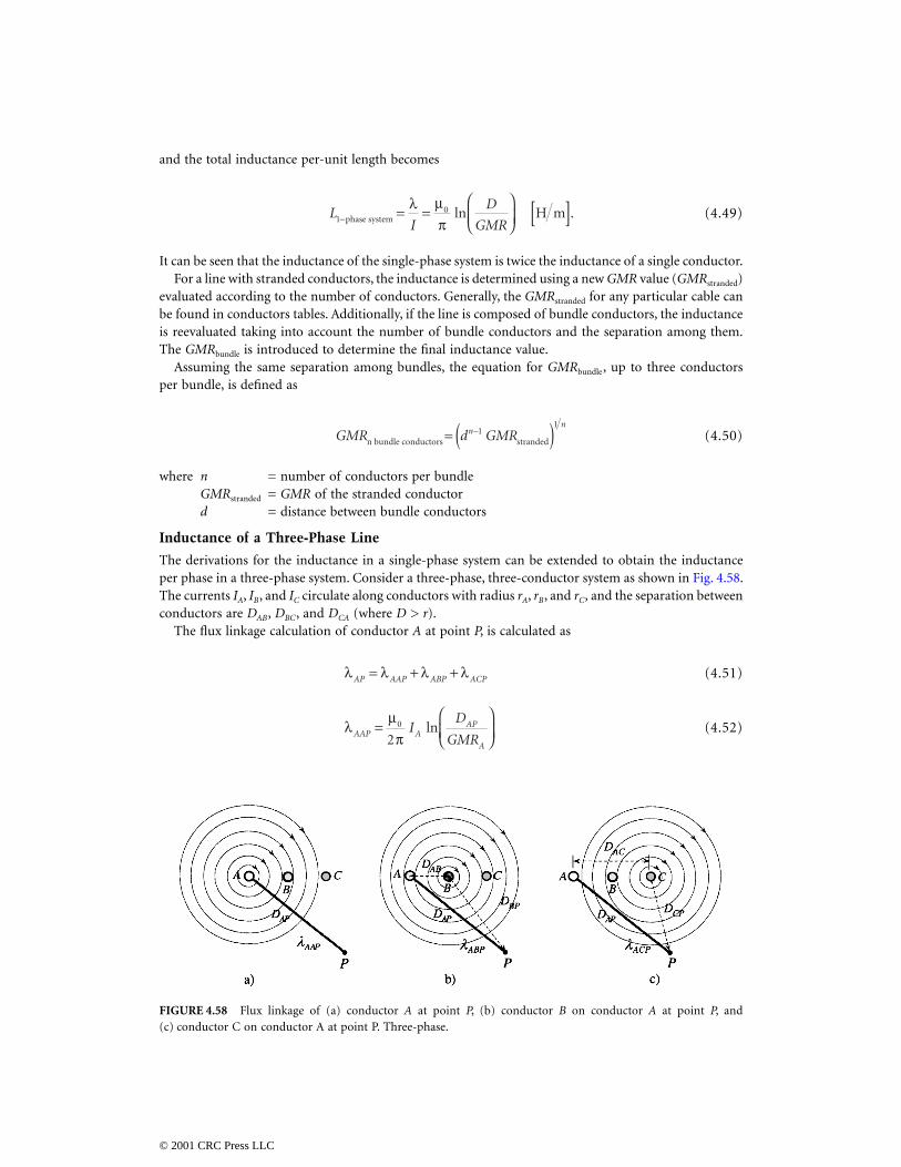
and the total inductance per-unit length becomes

(4.49)

It can be seen that the inductance of the single-phase system is twice the inductance of a single conductor.For a line with stranded conductors, the inductance is determined using a new GMR value (GMRstranded)

evaluated according to the number of conductors. Generally, the GMRstranded for any particular cable canbe found in conductors tables. Additionally, if the line is composed of bundle conductors, the inductanceis reevaluated taking into account the number of bundle conductors and the separation among them.The GMRbundle is introduced to determine the final inductance value.

Assuming the same separation among bundles, the equation for GMRbundle, up to three conductorsper bundle, is defined as

(4.50)

where n = number of conductors per bundleGMRstranded = GMR of the stranded conductord = distance between bundle conductors

Inductance of a Three-Phase Line

The derivations for the inductance in a single-phase system can be extended to obtain the inductanceper phase in a three-phase system. Consider a three-phase, three-conductor system as shown in Fig. 4.58.The currents IA, IB, and IC circulate along conductors with radius rA, rB, and rC, and the separation betweenconductors are DAB, DBC, and DCA (where D > r).

The flux linkage calculation of conductor A at point P, is calculated as

(4.51)

(4.52)

FIGURE 4.58 Flux linkage of (a) conductor A at point P, (b) conductor B on conductor A at point P, and(c) conductor C on conductor A at point P. Three-phase.

LI

D

GMR10

− = = µπ

[ ]phase system H mλ

ln .

GMR d GMRnn

n bundle conductors stranded= ( )−11

λ λ λ λAP AAP ABP ACP= + +

λAAP AAP

A

ID

GMR= µ

π

0

2ln


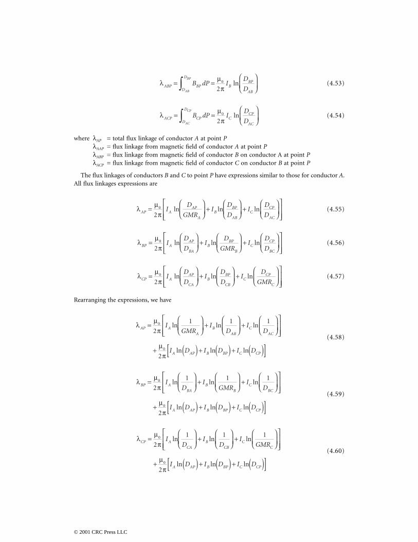
(4.53)

(4.54)

where λAP = total flux linkage of conductor A at point PλAAP = flux linkage from magnetic field of conductor A at point PλABP = flux linkage from magnetic field of conductor B on conductor A at point PλACP = flux linkage from magnetic field of conductor C on conductor B at point P

The flux linkages of conductors B and C to point P have expressions similar to those for conductor A.All flux linkages expressions are

(4.55)

(4.56)

(4.57)

Rearranging the expressions, we have

(4.58)

(4.59)

(4.60)

λABP BPD

D

BBP

AB

B dP ID

DAB

BP

= = µπ

∫ 0

2ln

λACP CPD

D

CCP

AC

B dP ID

DAC

CP

= = µπ

∫ 0

2ln

λAP AAP

A

BBP

AB

CCP

AC

ID

GMRI

D

DI

D

D= µ

π

+

+

0

2ln ln ln

λBP AAP

BA

BBP

B

CCP

BC

ID

DI

D

GMRI

D

D= µ

π

+

+

0

2ln ln ln

λCP AAP

CA

BBP

CB

CCP

C

ID

DI

D

DI

D

GMR= µ

π

+

+

0

2ln ln ln

λAP A

A

B

AB

C

AC

A AP B BP C CP

IGMR

ID

ID

I D I D I D

= µπ

+

+

+ µπ ( ) + ( ) + ( )[ ]

0

0

2

1 1 1

2

ln ln ln

ln ln ln

λBP A

BA

B

B

C

BC

A AP B BP C CP

ID

IGMR

ID

I D I D I D

= µπ

+

+

+ µπ ( ) + ( ) + ( )[ ]

0

0

2

1 1 1

2

ln ln ln

ln ln ln

λCP A

CA

B

CB

C

C

A AP B BP C CP

ID

ID

IGMR

I D I D I D

= µπ

+

+

+ µπ ( ) + ( ) + ( )[ ]

0

0

2

1 1 1

2

ln ln ln

ln ln ln


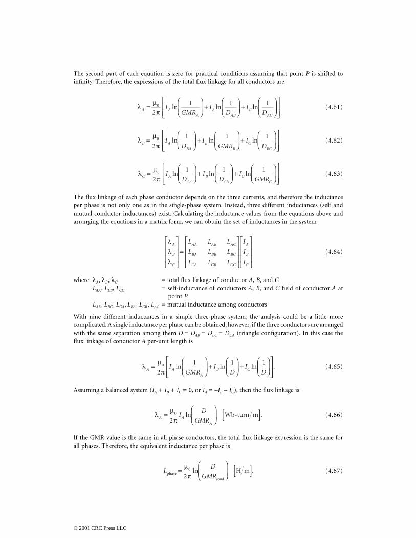
The second part of each equation is zero for practical conditions assuming that point P is shifted toinfinity. Therefore, the expressions of the total flux linkage for all conductors are

(4.61)

(4.62)

(4.63)

The flux linkage of each phase conductor depends on the three currents, and therefore the inductanceper phase is not only one as in the single-phase system. Instead, three different inductances (self andmutual conductor inductances) exist. Calculating the inductance values from the equations above andarranging the equations in a matrix form, we can obtain the set of inductances in the system

(4.64)

where λA, λB, λC = total flux linkage of conductor A, B, and CLAA, LBB, LCC = self-inductance of conductors A, B, and C field of conductor A at

point PLAB, LBC, LCA, LBA, LCB, LAC = mutual inductance among conductors

With nine different inductances in a simple three-phase system, the analysis could be a little morecomplicated. A single inductance per phase can be obtained, however, if the three conductors are arrangedwith the same separation among them D = DAB = DBC = DCA (triangle configuration). In this case theflux linkage of conductor A per-unit length is

(4.65)

Assuming a balanced system (IA + IB + IC = 0, or IA = –IB – IC), then the flux linkage is

(4.66)

If the GMR value is the same in all phase conductors, the total flux linkage expression is the same forall phases. Therefore, the equivalent inductance per phase is

(4.67)

λA A

A

B

AB

C

AC

IGMR

ID

ID

= µπ

+

+

0

2

1 1 1ln ln ln

λB A

BA

B

B

C

BC

ID

IGMR

ID

= µπ

+

+

0

2

1 1 1ln ln ln

λC A

CA

B

CB

C

C

ID

ID

IGMR

= µπ

+

+

0

2

1 1 1ln ln ln

λλλ

A

B

C

AA AB AC

BA BB BC

CA CB CC

A

B

C

L L L

L L L

L L L

I

I

I

=

λA A

A

B CIGMR

ID

ID

= µπ

+

+

0

2

1 1 1ln ln ln .

λA A

A

ID

GMR= µ

π

[ ]0

2ln .Wb-turn m

LD

GMRcond

phase H m= µπ

[ ]0

2ln .


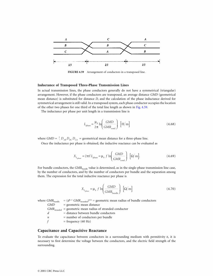
Inductance of Transposed Three-Phase Transmission Lines

In actual transmission lines, the phase conductors generally do not have a symmetrical (triangular)arrangement. However, if the phase conductors are transposed, an average distance GMD (geometricalmean distance) is substituted for distance D, and the calculation of the phase inductance derived forsymmetrical arrangement is still valid. In a transposed system, each phase conductor occupies the locationof the other two phases for one third of the total line length as shown in Fig. 4.59.

The inductance per phase per unit length in a transmission line is

(4.68)

where GMD = = geometrical mean distance for a three-phase line.

Once the inductance per phase is obtained, the inductive reactance can be evaluated as

(4.69)

For bundle conductors, the GMRbundle value is determined, as in the single-phase transmission line case,by the number of conductors, and by the number of conductors per bundle and the separation amongthem. The expression for the total inductive reactance per phase is

(4.70)

where GMRbundle = (dn–1 GMRstranded)1/n = geometric mean radius of bundle conductorsGMD = geometric mean distanceGMRstranded = geometric mean radius of stranded conductord = distance between bundle conductorsn = number of conductors per bundlef = frequency (60 Hz)

Capacitance and Capacitive Reactance

To evaluate the capacitance between conductors in a surrounding medium with permitivity ε, it isnecessary to first determine the voltage between the conductors, and the electric field strength of thesurrounding.

FIGURE 4.59 Arrangement of conductors in a transposed line.

LGMD

GMRphase

cond

H m= µπ

[ ]0

2ln

D D DAB BC CA3

X L fGMD

GMRL phase

condphase

f m= π = µ

[ ]2 0 ln .Ω

X fGMD

GMRL

bundlephase

m= µ

[ ]0 ln Ω


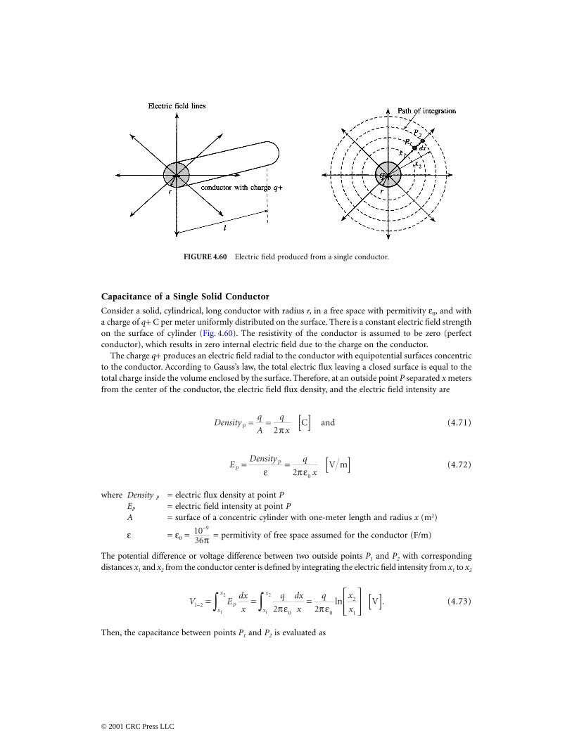
Capacitance of a Single Solid Conductor

Consider a solid, cylindrical, long conductor with radius r, in a free space with permitivity ε0, and witha charge of q+ C per meter uniformly distributed on the surface. There is a constant electric field strengthon the surface of cylinder (Fig. 4.60). The resistivity of the conductor is assumed to be zero (perfectconductor), which results in zero internal electric field due to the charge on the conductor.

The charge q+ produces an electric field radial to the conductor with equipotential surfaces concentricto the conductor. According to Gauss’s law, the total electric flux leaving a closed surface is equal to thetotal charge inside the volume enclosed by the surface. Therefore, at an outside point P separated x metersfrom the center of the conductor, the electric field flux density, and the electric field intensity are

(4.71)

(4.72)

where Density P = electric flux density at point PEP = electric field intensity at point PA = surface of a concentric cylinder with one-meter length and radius x (m2)

ε = ε0 = = permitivity of free space assumed for the conductor (F/m)

The potential difference or voltage difference between two outside points P1 and P2 with correspondingdistances x1 and x2 from the conductor center is defined by integrating the electric field intensity from x1 to x2

(4.73)

Then, the capacitance between points P1 and P2 is evaluated as

FIGURE 4.60 Electric field produced from a single conductor.

Densityq

A

q

xP = =π [ ]

2 C and

EDensity q

xPP= =

π [ ]ε ε2 0

V m

1036

9−

π

V Edx

x

q dx

x

q x

xPx

x

x

x

1 2

0 0

2

11

2

1

2

2 2− = =π

=π

[ ]∫ ∫ ε εln .V


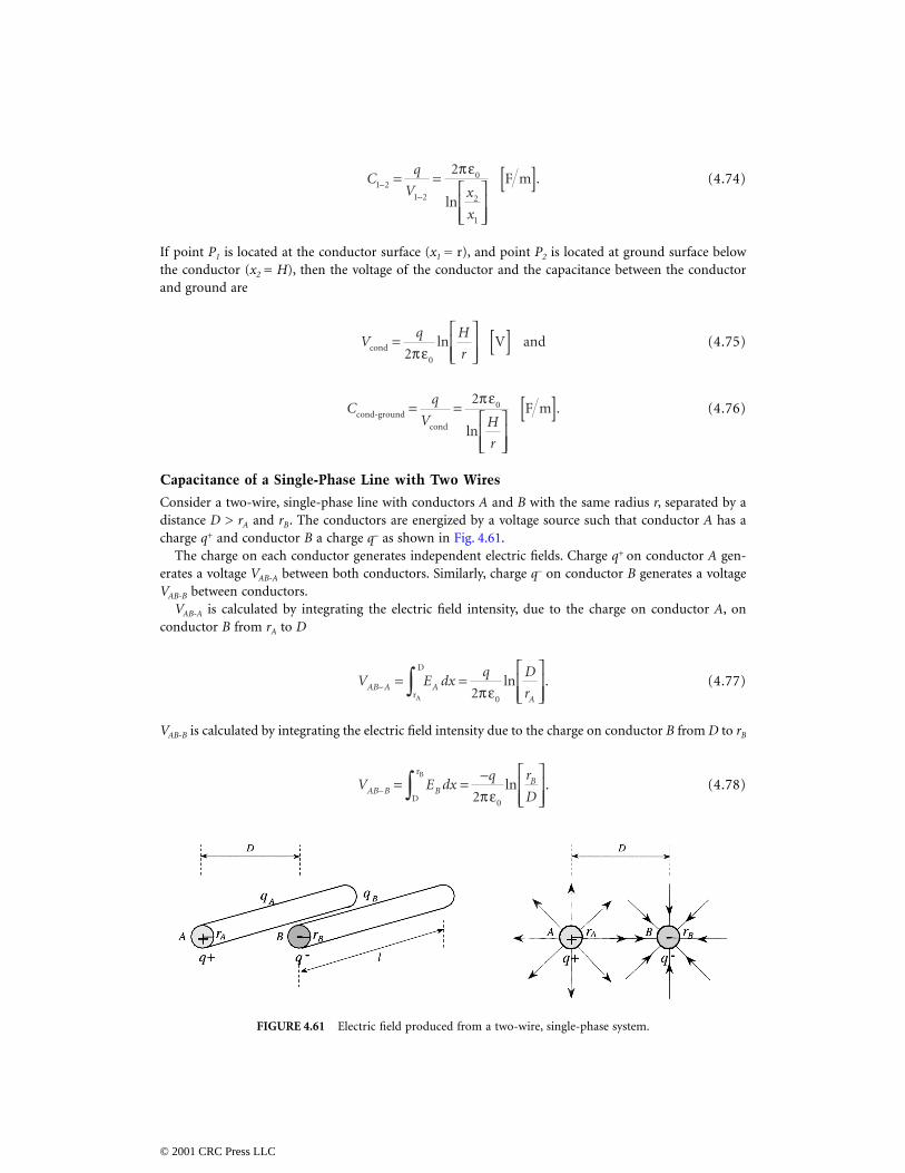
(4.74)

If point P1 is located at the conductor surface (x1 = r), and point P2 is located at ground surface belowthe conductor (x2 = H), then the voltage of the conductor and the capacitance between the conductorand ground are

(4.75)

(4.76)

Capacitance of a Single-Phase Line with Two Wires

Consider a two-wire, single-phase line with conductors A and B with the same radius r, separated by adistance D > rA and rB. The conductors are energized by a voltage source such that conductor A has acharge q+ and conductor B a charge q– as shown in Fig. 4.61.

The charge on each conductor generates independent electric fields. Charge q+ on conductor A gen-erates a voltage VAB-A between both conductors. Similarly, charge q– on conductor B generates a voltageVAB-B between conductors.

VAB-A is calculated by integrating the electric field intensity, due to the charge on conductor A, onconductor B from rA to D

(4.77)

VAB-B is calculated by integrating the electric field intensity due to the charge on conductor B from D to rB

(4.78)

FIGURE 4.61 Electric field produced from a two-wire, single-phase system.

Cq

V x

x

1 2

1 2

0

2

1

2−

−

= = π

[ ]ε

ln

.F m

Vq H

rcond V and=π

[ ]2 0ε

ln

Cq

V H

r

cond-ground

cond

F m= = π

[ ]2 0ε

ln

.

V E dxq D

rAB A A

A

− = =π

∫r

D

A 2 0εln .

V E dxq r

DAB B BB

− = = −π

∫D

rB

2 0εln .


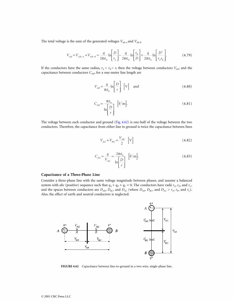
The total voltage is the sum of the generated voltages VAB-A and VAB-B

(4.79)

If the conductors have the same radius, rA = rB = r, then the voltage between conductors VAB, and thecapacitance between conductors CAB, for a one-meter line length are

(4.80)

(4.81)

The voltage between each conductor and ground (Fig. 4.62) is one-half of the voltage between the twoconductors. Therefore, the capacitance from either line to ground is twice the capacitance between lines

(4.82)

(4.83)

Capacitance of a Three-Phase Line

Consider a three-phase line with the same voltage magnitude between phases, and assume a balancedsystem with abc (positive) sequence such that qA + qB + qC = 0. The conductors have radii rA, rB, and rC,and the spaces between conductors are DAB, DBC, and DAC (where DAB, DBC, and DAC > rA, rB, and rC).Also, the effect of earth and neutral conductors is neglected.

FIGURE 4.62 Capacitance between line-to-ground in a two-wire, single-phase line.

V V Vq D

r

q r

D

q D

r rAB AB A AB B

A

B

A B

= + =π

−π

=π

− − 2 2 20 0 0

2

ε ε εln ln ln .

Vq D

rAB =π

[ ]ε0

ln V and

CD

r

AB = π

[ ]ε0

ln

.F m

V VV

AG BGAB= = [ ]2

V

Cq

V D

r

AG

AG

= = π

[ ]2 0ε

ln

.F m


The expression for voltage between two conductors in a single-phase system can be extended to obtainthe voltages between conductors in a three-phase system. The expressions for VAB and VAC are

(4.84)

(4.85)

If the three-phase system has a triangular arrangement with equidistant conductors such that DAB = DBC =DAC = D, with the same radii for the conductors such that rA = rB = rC = r (where D > r), the expressionsfor VAB and VAC are

(4.86)

(4.87)

Balanced line-to-line voltages with sequence abc, expressed in terms of the line-to-neutral voltage are:

, and ; where VAN is the line-to-neutral voltage. There-

fore, VAN can be expressed in terms of VAB and VAC as

(4.88)

and thus, substituting VAB and VAC from Eqs. (4.81) and (4.82), we have

(4.89)

Under balanced conditions (qA + qB + qC = 0, or –qA = (qB + qC) then, the final expression for the line-to-neutral voltage is

V qD

rq

r

Dq

D

DAB AAB

A

BB

AB

CBC

AC

=π

+

+

1

2 0εln ln ln and

V qD

rq

D

Dq

r

DAC ACA

A

BBC

AB

CC

AC

=π

+

+

1

2 0εln ln ln

V qD

rq

r

Dq

D

D

qD

rq

r

D

AB A B C

A B

=π

+

+

=π

+

[ ]

1

2

1

2

0

0

ε

ε

ln ln ln

ln ln V

V qD

rq

D

Dq

r

D

qD

rq

r

D

AC A B C

A C

=π

+

+

=π

+

[ ]

1

2

1

2

0

0

ε

ε

ln ln ln

ln ln V

V VAB AN= ∠ °3 30 V V VAC CA AN= − = ∠ − °3 30

VV V

ANAB AC= +

3

V qD

rq

r

Dq

D

rq

r

D

qD

rq q

r

AN A B A C

A B C

=π

+

+

+

=π

+ +( )

1

6

1

62

0

0

ε

ε

ln ln ln ln

ln lnDD

.


(4.90)

The positive sequence capacitance per unit length between phase A and neutral can now be obtained.The same result is obtained for capacitance between phases B and C to neutral.

(4.91)

Capacitance of Stranded Bundle Conductors

The calculation of the capacitance in the equation above is based on:

1. solid conductors with zero resistivity (zero internal electric field)2. distributed charge uniformly3. equilateral spacing of phase conductors

In actual transmission lines, the resistivity of the conductors produces a small internal electric field and,therefore, the electric field at the conductor surface is smaller than estimated. However, the difference isnegligible for practical purposes. Because of the presence of other charged conductors, the chargedistribution is nonuniform, and therefore the estimated capacitance is different. However, this effect isnegligible for most practical calculations. In a line with stranded conductors, the capacitance is evaluatedassuming a solid conductor with the same radius as the outside radius of the stranded conductor. Thisproduces a negligible difference.

Most transmission lines do not have equilateral spacing of phase conductors. This causes differencesbetween the line-to-neutral capacitances of the three phases. However, transposing the phase conductorsbalances the system, resulting in equal line-to-neutral capacitance for each phase and is developed in thefollowing manner.

Consider a transposed three-phase line with conductors having the same radius r, and with spacebetween conductors DAB, DBC, and DAC, where DAB, DBC, and DAC > r. Assuming abc positive sequence,the expressions for VAB on the first, second, and third sections of the transposed line are

(4.92)

(4.93)

(4.94)

Similarly, the expressions for VAC on the first, second, and third sections of the transposed line are

(4.95)

V qD

rAN A=π

[ ]1

2 0εln .V

Cq

V D

r

ANA

AN

= = π

[ ]2 0ε

ln

F m

V qD

rq

r

Dq

D

DAB AAB

B

AB

CAB

AC

first =π

+

+

1

2 0εln ln ln

V qD

rq

r

Dq

D

DAB ABC

B

BC

CAC

AB

second =π

+

+

1

2 0εln ln ln

V qD

rq

r

Dq

D

DAB AAC

B

AC

CAB

BC

third =π

+

+

1

2 0εln ln ln .

V qD

rq

D

Dq

r

DAC AAC

BBC

AB

C

AC

first =π

+

+

1

2 0εln ln ln


(4.96)

(4.97)

Taking the average value of the three sections, we have the final expressions of VAB and VAC in thetransposed line

(4.98)

(4.99)

For a balanced system where –qA = (qB + qC), the phase-to-neutral voltage VAN (phase voltage) is

(4.100)

where GMD = = geometrical mean distance for a three-phase line.

For bundle conductors, an equivalent radius re replaces the radius r of a single conductor and isdetermined by the number of conductors per bundle and the spacing of conductors. The expression ofre is similar to GMRbundle used in the calculation of the inductance per phase, except that the actual outsideradius of the conductor is used instead of the GMRcond. Therefore, the expression for VAN is

(4.101)

where re = (dn–1 r)1/n = equivalent radius for up to three conductors per bundle (m)d = distance between bundle conductors (m)n = number of conductors per bundle

V qD

rq

D

Dq

r

DAC AAB

BAC

BC

C

AB

second =π

+

+

1

2 0εln ln ln

V qD

rq

D

Dq

r

DAC ABC

BAB

AC

C

BC

third =π

+

+

1

2 0εln ln ln

VV V V

qD D D

rq

r

D D Dq

D D D

D D D

AB

AB AB AB

AAB AC BC

B

AB AC BC

CAC AC BC

AC AC BC

transp

first second third=+ +

=π

+

+

3

1

6 03

3

εln ln ln

VV V V

qD D D

rq

D D D

D D Dq

r

D D D

AB

AC AC AC

AAB AC BC

BAC AC BC

AB AC BC

C

AC AC BC

transp

first second third=+ +

=π

+

+

3

1

6 03

3

εln ln ln .

VV V

qD D D

rq q

r

D D D

qD D D

rq

GMD

r

AN

AB AC

A

AB AC BC

B C

AB AC BC

A

AB AC BC

A

transp

transp transp=+

=π

+ +( )

=π

=π

3

1

182

1

6

1

2

03

3

03

0

ε

ε ε

ln ln

ln ln V[ ]

D D DAB BC CA3

V qGMD

rAN A

e

transp V=π

[ ]1

2 0εln


Finally, the capacitance and capacitive reactance per unit length from phase to neutral can be evaluated as

(4.102)

(4.103)

Characteristics of Overhead Conductors

Tables 4.9a and 4.9b present general characteristics of aluminum cable steel reinforced conductors(ACSR). The size of the conductors (cross-section area) is specified in square millimeters and kcmil,where a cmil is the cross-section area of a circular conductor with a diameter of 1/1000 inch. Typicalvalues of resistance, inductive reactance, and capacitive reactance are listed. The approximate current-carrying capacity of the conductors is also included assuming 60 Hz, wind speed of 1.4 mi/h, andconductor and air temperatures of 75°C and 25°C, respectively. Similarly, Tables 4.10a and 4.10b presentthe corresponding characteristics of aluminum conductors (AAC).

References

Barnes, C. C., Power Cables: Their Design and Installation, 2nd ed., Chapman and Hall, Ltd., London, 1966.Electric Power Research Institute, Transmission Line Reference Book 345 kV and Above, 2nd ed., Palo Alto,

CA, 1987.Glover J. D., Sarma, M., and Digby, G., Power System Analysis and Design with Personal Computer

Applications, 2nd ed., PWS Publishing Company, 1994.Gross, Ch. A., Power System Analysis, John Wiley & Sons, New York, 1979.Gungor, B. R., Power Systems, Harcourt Brace Jovanovich, Florida, 1988.Yamayee, Z. A., and Bala, J. L. Jr., Electromechanical Energy Devices and Power Systems, John Wiley &

Sons, New York, 1994.Zaborszky, J., and Rittenhouse, J. W., Electric Power Transmission: The Power System in the Steady State,

The Ronald Press Company, New York, 1954.

Cq

V GMD

r

ANA

AN

e

transp

transp

F m= = π

[ ]2 0ε

ln

XC

GMD

rAN

AN e

transp

transpf fm=

π=

π

[ ]1

2

1

4 0εln .Ω


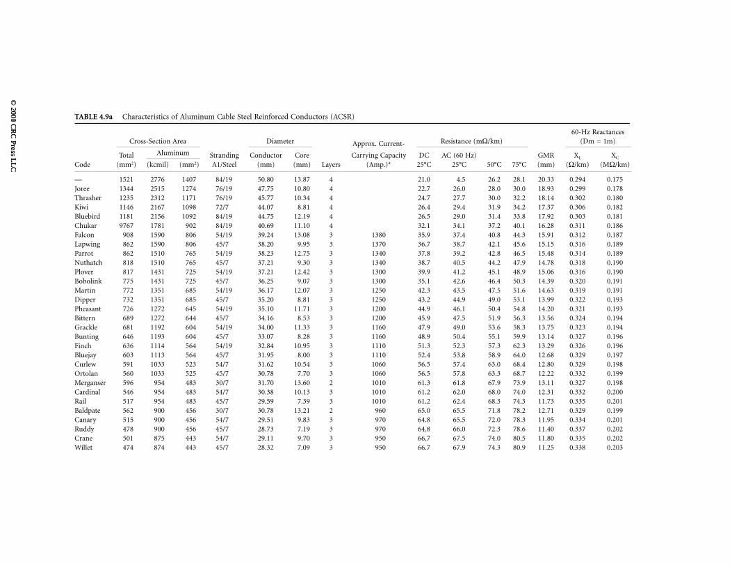
TABLE 4.9a Characteristics of Aluminum Cable Steel Reinforced Conductors (ACSR)

Cross-Section Area Diameter Approx. Current- Resistance (mΩ/km)60-Hz Reactances

(Dm = 1m)

Total Aluminum Stranding Conductor Core Carrying Capacity DC AC (60 Hz) GMR XL XC

Code (mm2) (kcmil) (mm2) A1/Steel (mm) (mm) Layers (Amp.)* 25°C 25°C 50°C 75°C (mm) (Ω/km) (MΩ/km)

— 1521 2776 1407 84/19 50.80 13.87 4 21.0 4.5 26.2 28.1 20.33 0.294 0.175Joree 1344 2515 1274 76/19 47.75 10.80 4 22.7 26.0 28.0 30.0 18.93 0.299 0.178Thrasher 1235 2312 1171 76/19 45.77 10.34 4 24.7 27.7 30.0 32.2 18.14 0.302 0.180Kiwi 1146 2167 1098 72/7 44.07 8.81 4 26.4 29.4 31.9 34.2 17.37 0.306 0.182Bluebird 1181 2156 1092 84/19 44.75 12.19 4 26.5 29.0 31.4 33.8 17.92 0.303 0.181Chukar 9767 1781 902 84/19 40.69 11.10 4 32.1 34.1 37.2 40.1 16.28 0.311 0.186Falcon 908 1590 806 54/19 39.24 13.08 3 1380 35.9 37.4 40.8 44.3 15.91 0.312 0.187Lapwing 862 1590 806 45/7 38.20 9.95 3 1370 36.7 38.7 42.1 45.6 15.15 0.316 0.189Parrot 862 1510 765 54/19 38.23 12.75 3 1340 37.8 39.2 42.8 46.5 15.48 0.314 0.189Nuthatch 818 1510 765 45/7 37.21 9.30 3 1340 38.7 40.5 44.2 47.9 14.78 0.318 0.190Plover 817 1431 725 54/19 37.21 12.42 3 1300 39.9 41.2 45.1 48.9 15.06 0.316 0.190Bobolink 775 1431 725 45/7 36.25 9.07 3 1300 35.1 42.6 46.4 50.3 14.39 0.320 0.191Martin 772 1351 685 54/19 36.17 12.07 3 1250 42.3 43.5 47.5 51.6 14.63 0.319 0.191Dipper 732 1351 685 45/7 35.20 8.81 3 1250 43.2 44.9 49.0 53.1 13.99 0.322 0.193Pheasant 726 1272 645 54/19 35.10 11.71 3 1200 44.9 46.1 50.4 54.8 14.20 0.321 0.193Bittern 689 1272 644 45/7 34.16 8.53 3 1200 45.9 47.5 51.9 56.3 13.56 0.324 0.194Grackle 681 1192 604 54/19 34.00 11.33 3 1160 47.9 49.0 53.6 58.3 13.75 0.323 0.194Bunting 646 1193 604 45/7 33.07 8.28 3 1160 48.9 50.4 55.1 59.9 13.14 0.327 0.196Finch 636 1114 564 54/19 32.84 10.95 3 1110 51.3 52.3 57.3 62.3 13.29 0.326 0.196Bluejay 603 1113 564 45/7 31.95 8.00 3 1110 52.4 53.8 58.9 64.0 12.68 0.329 0.197Curlew 591 1033 523 54/7 31.62 10.54 3 1060 56.5 57.4 63.0 68.4 12.80 0.329 0.198Ortolan 560 1033 525 45/7 30.78 7.70 3 1060 56.5 57.8 63.3 68.7 12.22 0.332 0.199Merganser 596 954 483 30/7 31.70 13.60 2 1010 61.3 61.8 67.9 73.9 13.11 0.327 0.198Cardinal 546 954 483 54/7 30.38 10.13 3 1010 61.2 62.0 68.0 74.0 12.31 0.332 0.200Rail 517 954 483 45/7 29.59 7.39 3 1010 61.2 62.4 68.3 74.3 11.73 0.335 0.201Baldpate 562 900 456 30/7 30.78 13.21 2 960 65.0 65.5 71.8 78.2 12.71 0.329 0.199Canary 515 900 456 54/7 29.51 9.83 3 970 64.8 65.5 72.0 78.3 11.95 0.334 0.201Ruddy 478 900 456 45/7 28.73 7.19 3 970 64.8 66.0 72.3 78.6 11.40 0.337 0.202Crane 501 875 443 54/7 29.11 9.70 3 950 66.7 67.5 74.0 80.5 11.80 0.335 0.202Willet 474 874 443 45/7 28.32 7.09 3 950 66.7 67.9 74.3 80.9 11.25 0.338 0.203

© 2000 C

RC

Press LL

C ©

2001 CR

C Press L

LC

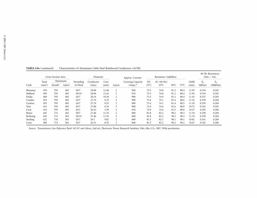
Skimmer 479 795 403 30/7 29.00 12.40 2 940 73.5 74.0 81.2 88.4 11.95 0.334 0.202Mallard 495 795 403 30/19 28.96 12.42 2 910 73.5 74.0 81.2 88.4 11.95 0.334 0.202Drake 469 795 403 26/7 28.14 10.36 2 900 73.3 74.0 81.2 88.4 11.43 0.337 0.203Condor 455 795 403 54/7 27.74 9.25 3 900 73.4 74.1 81.4 88.6 11.22 0.339 0.204Cuckoo 455 795 403 24/7 27.74 9.25 2 900 73.4 74.1 81.4 88.5 11.16 0.339 0.204Tern 431 795 403 45/7 27.00 6.76 3 900 73.4 74.4 81.6 88.8 10.73 0.342 0.205Coot 414 795 403 36/1 26.42 3.78 3 910 73.0 74.4 81.5 88.6 10.27 0.345 0.206Buteo 447 715 362 30/7 27.46 11.76 2 840 81.8 82.2 90.2 98.3 11.34 0.338 0.204Redwing 445 715 362 30/19 27.46 11.76 2 840 81.8 82.2 90.2 98.3 11.34 0.338 0.204Starling 422 716 363 26/7 26.7 9.82 2 840 81.5 82.1 90.1 98.1 10.82 0.341 0.206Crow 409 715 362 54/7 26.31 8.76 3 840 81.5 82.2 90.2 98.2 10.67 0.342 0.206

Source: Transmission Line Reference Book 345 kV and Above, 2nd ed., Electronic Power Research Institute, Palo Alto, CA, 1987. With permission.

TABLE 4.9a (continued) Characteristics of Aluminum Cable Steel Reinforced Conductors (ACSR)


(Dm = 1m)



©

2001 CR

C Press L

LC

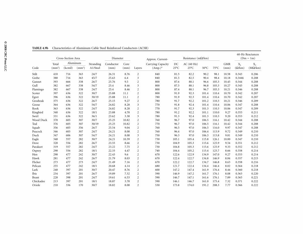
TABLE 4.9b Characteristics of Aluminum Cable Steel Reinforced Conductors (ACSR)


(Dm = 1m)



Stilt 410 716 363 24/7 26.31 8.76 2 840 81.5 82.2 90.2 98.1 10.58 0.343 0.206Grebe 388 716 363 45/7 25.63 6.4 3 840 81.5 82.5 90.4 98.4 10.18 0.3446 0.208Gannet 393 666 338 26/7 25.76 9.5 2 800 87.6 88.1 96.6 105.3 10.45 0.344 0.208Gull 382 667 338 54/7 25.4 8.46 3 800 87.5 88.1 96.8 105.3 10.27 0.345 0.208Flamingo 382 667 338 24/7 25.4 8.46 2 800 87.4 88.1 96.7 105.3 10.21 0.346 0.208Scoter 397 636 322 30/7 25.88 11.1 2 800 91.9 92.3 101.4 110.4 10.70 0.342 0.207Egret 396 636 322 30/19 25.88 11.1 2 780 91.9 92.3 101.4 110.4 10.70 0.342 0.207Grosbeak 375 636 322 26/7 25.15 9.27 2 780 91.7 92.2 101.2 110.3 10.21 0.346 0.209Goose 364 636 322 54/7 24.82 8.28 3 770 91.8 92.4 101.4 110.4 10.06 0.347 0.208Rook 363 636 322 24/7 24.82 8.28 2 770 91.7 92.3 101.3 110.3 10.06 0.347 0.209Kingbird 340 636 322 18/1 23.88 4.78 2 780 91.2 92.2 101.1 110.0 9.27 0.353 0.211Swirl 331 636 322 36/1 23.62 3.38 3 780 91.3 92.4 101.3 110.3 9.20 0.353 0.212Wood Duck 378 605 307 30/7 25.25 10.82 2 760 96.7 97.0 106.5 116.1 10.42 0.344 0.208Teal 376 605 307 30/19 25.25 10.82 2 770 96.7 97.0 106.5 116.1 10.42 0.344 0.208Squab 356 605 356 26/7 25.54 9.04 2 760 96.5 97.0 106.5 116.0 9.97 0.347 0.208Peacock 346 605 307 24/7 24.21 8.08 2 760 96.4 97.0 106.4 115.9 9.72 0.349 0.210Duck 347 606 307 54/7 24.21 8.08 3 750 96.3 97.0 106.3 115.8 9.81 0.349 0.210Eagle 348 557 282 30/7 24.21 10.39 2 730 105.1 105.4 115.8 126.1 10.00 0.347 0.210Dove 328 556 282 26/7 23.55 8.66 2 730 104.9 105.3 115.6 125.9 9.54 0.351 0.212Parakeet 319 557 282 24/7 23.22 7.75 2 730 104.8 105.3 115.6 125.9 9.33 0.352 0.212Osprey 298 556 282 18/1 22.33 4.47 2 740 104.4 105.2 115.4 125.7 8.66 0.358 0.214Hen 298 477 242 30/7 22.43 9.6 2 670 122.6 122.9 134.9 147.0 9.27 0.353 0.214Hawk 281 477 242 26/7 21.79 8.03 2 670 122.4 122.7 134.8 146.9 8.84 0.357 0.215Flicker 273 477 273 24/7 21.49 7.16 2 670 122.2 122.7 134.7 146.8 8.63 0.358 0.216Pelican 255 477 242 18/1 20.68 4.14 2 680 121.7 122.4 134.4 146.4 8.02 0.364 0.218Lark 248 397 201 30/7 20.47 8.76 2 600 147.2 147.4 161.9 176.4 8.44 0.360 0.218Ibis 234 397 201 26/7 19.89 7.32 2 590 146.9 147.2 161.7 176.1 8.08 0.363 0.220Brant 228 398 201 24/7 19.61 6.53 2 590 146.7 147.1 161.6 176.1 7.89 0.365 0.221Chickadee 213 397 201 18/1 18.87 3.78 2 590 146.1 146.7 161.0 175.4 7.32 0.371 0.222Oriole 210 336 170 30/7 18.82 8.08 2 530 173.8 174.0 191.2 208.3 7.77 0.366 0.222

© 2000 C

RC

Press LL

C ©

2001 CR

C Press L

LC

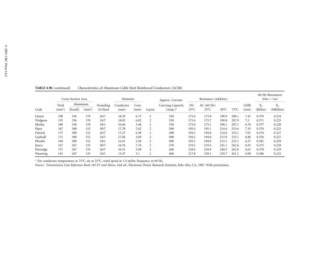
Linnet 198 336 170 26/7 18.29 6.73 2 530 173.6 173.8 190.9 208.1 7.41 0.370 0.224Widgeon 193 336 170 24/7 18.03 6.02 2 530 173.4 173.7 190.8 207.9 7.5 0.371 0.225Merlin 180 336 170 18/1 16.46 3.48 2 530 173.0 173.1 190.1 207.1 6.74 0.377 0.220Piper 187 300 152 30/7 17.78 7.62 2 500 195.0 195.1 214.4 233.6 7.35 0.370 0.225Ostrich 177 300 152 26/7 17.27 6.38 2 490 194.5 194.8 214.0 233.1 7.01 0.374 0.227Gadwall 172 300 152 24/7 17.04 5.69 2 490 194.5 194.8 213.9 233.1 6.86 0.376 0.227Phoebe 160 300 152 18/1 16.41 3.28 2 490 193.5 194.0 213.1 232.1 6.37 0.381 0.229Junco 167 267 135 30/7 16.76 7.19 2 570 219.2 219.4 241.1 262.6 6.92 0.375 0.228Partridge 157 267 135 26/7 16.31 5.99 2 460 218.6 218.9 240.5 262.0 6.61 0.378 0.229Waxwing 143 267 135 18/1 15.47 3.1 2 460 217.8 218.1 239.7 261.1 6.00 0.386 0.232

* For conductor temperature at 75°C, air at 25°C, wind speed at 1.4 mi/hr, frequency at 60 Hz.Source: Transmission Line Reference Book 345 kV and Above, 2nd ed., Electronic Power Research Institute, Palo Alto, CA, 1987. With permission.

TABLE 4.9b (continued) Characteristics of Aluminum Cable Steel Reinforced Conductors (ACSR)


(Dm = 1m)



©

2001 CR

C Press L

LC

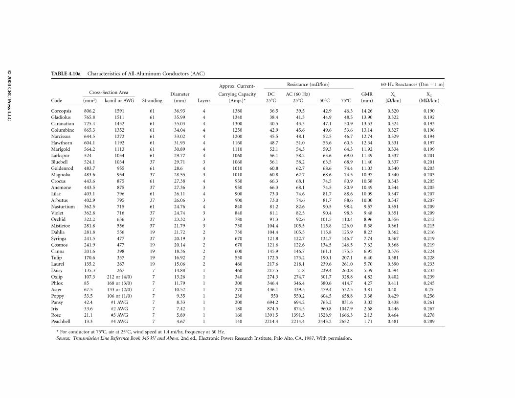
TABLE 4.10a Characteristics of All-Aluminum Conductors (AAC)

Approx. Current- Resistance (mΩ/km) 60-Hz Reactances (Dm = 1 m)

Cross-Section Area Diameter Carrying Capacity DC AC (60 Hz) GMR XL XC

Code (mm2) kcmil or AWG Stranding (mm) Layers (Amp.)* 25°C 25°C 50°C 75°C (mm) (Ω/km) (MΩ/km)

Coreopsis 806.2 1591 61 36.93 4 1380 36.5 39.5 42.9 46.3 14.26 0.320 0.190Gladiolus 765.8 1511 61 35.99 4 1340 38.4 41.3 44.9 48.5 13.90 0.322 0.192Caranation 725.4 1432 61 35.03 4 1300 40.5 43.3 47.1 50.9 13.53 0.324 0.193Columbine 865.3 1352 61 34.04 4 1250 42.9 45.6 49.6 53.6 13.14 0.327 0.196Narcissus 644.5 1272 61 33.02 4 1200 45.5 48.1 52.5 46.7 12.74 0.329 0.194Hawthorn 604.1 1192 61 31.95 4 1160 48.7 51.0 55.6 60.3 12.34 0.331 0.197Marigold 564.2 1113 61 30.89 4 1110 52.1 54.3 59.3 64.3 11.92 0.334 0.199Larkspur 524 1034 61 29.77 4 1060 56.1 58.2 63.6 69.0 11.49 0.337 0.201Bluebell 524.1 1034 37 29.71 3 1060 56.1 58.2 63.5 68.9 11.40 0.337 0.201Goldenrod 483.7 955 61 28.6 4 1010 60.8 62.7 68.6 74.4 11.03 0.340 0.203Magnolia 483.6 954 37 28.55 3 1010 60.8 62.7 68.6 74.5 10.97 0.340 0.203Crocus 443.6 875 61 27.38 4 950 66.3 68.1 74.5 80.9 10.58 0.343 0.205Anemone 443.5 875 37 27.36 3 950 66.3 68.1 74.5 80.9 10.49 0.344 0.205Lilac 403.1 796 61 26.11 4 900 73.0 74.6 81.7 88.6 10.09 0.347 0.207Arbutus 402.9 795 37 26.06 3 900 73.0 74.6 81.7 88.6 10.00 0.347 0.207Nasturtium 362.5 715 61 24.76 4 840 81.2 82.6 90.5 98.4 9.57 0.351 0.209Violet 362.8 716 37 24.74 3 840 81.1 82.5 90.4 98.3 9.48 0.351 0.209Orchid 322.2 636 37 23.32 3 780 91.3 92.6 101.5 110.4 8.96 0.356 0.212Mistletoe 281.8 556 37 21.79 3 730 104.4 105.5 115.8 126.0 8.38 0.361 0.215Dahlia 281.8 556 19 21.72 2 730 104.4 105.5 115.8 125.9 8.23 0.362 0.216Syringa 241.5 477 37 20.19 3 670 121.8 122.7 134.7 146.7 7.74 0.367 0.219Cosmos 241.9 477 19 20.14 2 670 121.6 122.6 134.5 146.5 7.62 0.368 0.219Canna 201.6 398 19 18.36 2 600 145.9 146.7 161.1 175.5 6.95 0.376 0.224Tulip 170.6 337 19 16.92 2 530 172.5 173.2 190.1 207.1 6.40 0.381 0.228Laurel 135.2 267 19 15.06 2 460 217.6 218.1 239.6 261.0 5.70 0.390 0.233Daisy 135.3 267 7 14.88 1 460 217.5 218 239.4 260.8 5.39 0.394 0.233Oxlip 107.3 212 or (4/0) 7 13.26 1 340 274.3 274.7 301.7 328.8 4.82 0.402 0.239Phlox 85 168 or (3/0) 7 11.79 1 300 346.4 346.4 380.6 414.7 4.27 0.411 0.245Aster 67.5 133 or (2/0) 7 10.52 1 270 436.1 439.5 479.4 522.5 3.81 0.40 0.25Poppy 53.5 106 or (1/0) 7 9.35 1 230 550 550.2 604.5 658.8 3.38 0.429 0.256Pansy 42.4 #1 AWG 7 8.33 1 200 694.2 694.2 763.2 831.6 3.02 0.438 0.261Iris 33.6 #2 AWG 7 7.42 1 180 874.5 874.5 960.8 1047.9 2.68 0.446 0.267Rose 21.1 #3 AWG 7 5.89 1 160 1391.5 1391.5 1528.9 1666.3 2.13 0.464 0.278Peachbell 13.3 #4 AWG 7 4.67 1 140 2214.4 2214.4 2443.2 2652 1.71 0.481 0.289

* For conductor at 75°C, air at 25°C, wind speed at 1.4 mi/hr, frequency at 60 Hz.Source: Transmission Line Reference Book 345 kV and Above, 2nd ed., Electronic Power Research Institute, Palo Alto, CA, 1987. With permission.

© 2000 C

RC

Press LL

C ©

2001 CR

C Press L

LC

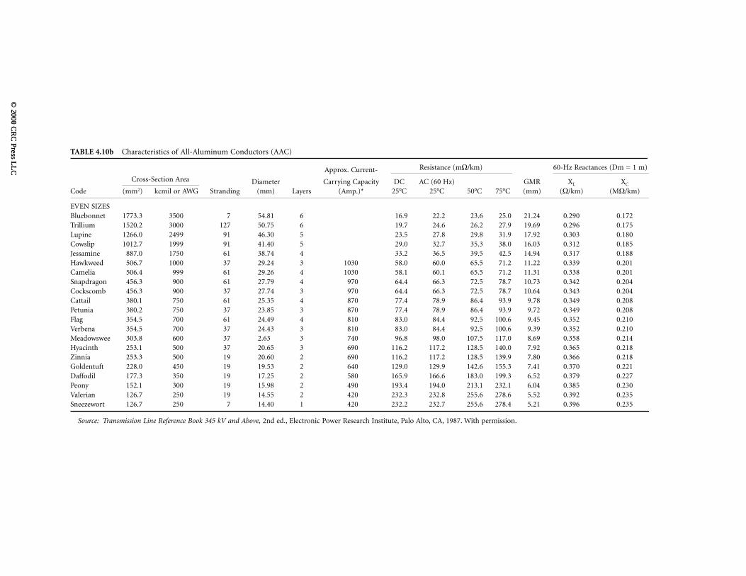
TABLE 4.10b Characteristics of All-Aluminum Conductors (AAC)

Approx. Current- Resistance (mΩ/km) 60-Hz Reactances (Dm = 1 m)

Cross-Section Area Diameter Carrying Capacity DC AC (60 Hz) GMR XL XC

Code (mm2) kcmil or AWG Stranding (mm) Layers (Amp.)* 25°C 25°C 50°C 75°C (mm) (Ω/km) (MΩ/km)

EVEN SIZESBluebonnet 1773.3 3500 7 54.81 6 16.9 22.2 23.6 25.0 21.24 0.290 0.172Trillium 1520.2 3000 127 50.75 6 19.7 24.6 26.2 27.9 19.69 0.296 0.175Lupine 1266.0 2499 91 46.30 5 23.5 27.8 29.8 31.9 17.92 0.303 0.180Cowslip 1012.7 1999 91 41.40 5 29.0 32.7 35.3 38.0 16.03 0.312 0.185Jessamine 887.0 1750 61 38.74 4 33.2 36.5 39.5 42.5 14.94 0.317 0.188Hawkweed 506.7 1000 37 29.24 3 1030 58.0 60.0 65.5 71.2 11.22 0.339 0.201Camelia 506.4 999 61 29.26 4 1030 58.1 60.1 65.5 71.2 11.31 0.338 0.201Snapdragon 456.3 900 61 27.79 4 970 64.4 66.3 72.5 78.7 10.73 0.342 0.204Cockscomb 456.3 900 37 27.74 3 970 64.4 66.3 72.5 78.7 10.64 0.343 0.204Cattail 380.1 750 61 25.35 4 870 77.4 78.9 86.4 93.9 9.78 0.349 0.208Petunia 380.2 750 37 23.85 3 870 77.4 78.9 86.4 93.9 9.72 0.349 0.208Flag 354.5 700 61 24.49 4 810 83.0 84.4 92.5 100.6 9.45 0.352 0.210Verbena 354.5 700 37 24.43 3 810 83.0 84.4 92.5 100.6 9.39 0.352 0.210Meadowswee 303.8 600 37 2.63 3 740 96.8 98.0 107.5 117.0 8.69 0.358 0.214Hyacinth 253.1 500 37 20.65 3 690 116.2 117.2 128.5 140.0 7.92 0.365 0.218Zinnia 253.3 500 19 20.60 2 690 116.2 117.2 128.5 139.9 7.80 0.366 0.218Goldentuft 228.0 450 19 19.53 2 640 129.0 129.9 142.6 155.3 7.41 0.370 0.221Daffodil 177.3 350 19 17.25 2 580 165.9 166.6 183.0 199.3 6.52 0.379 0.227Peony 152.1 300 19 15.98 2 490 193.4 194.0 213.1 232.1 6.04 0.385 0.230Valerian 126.7 250 19 14.55 2 420 232.3 232.8 255.6 278.6 5.52 0.392 0.235Sneezewort 126.7 250 7 14.40 1 420 232.2 232.7 255.6 278.4 5.21 0.396 0.235

Source: Transmission Line Reference Book 345 kV and Above, 2nd ed., Electronic Power Research Institute, Palo Alto, CA, 1987. With permission.

© 2000 C

RC

Press LL

C ©

2001 CR

C Press L

LC

4.7 Sag and Tension of Conductor

D.A. Douglass and Ridley Thrash

The energized conductors of transmission and distribution lines must be placed to totally eliminate thepossibility of injury to people. Overhead conductors, however, elongate with time, temperature, andtension, thereby changing their original positions after installation. Despite the effects of weather andloading on a line, the conductors must remain at safe distances from buildings, objects, and people orvehicles passing beneath the line at all times. To ensure this safety, the shape of the terrain along theright-of-way, the height and lateral position of the conductor support points, and the position of theconductor between support points under all wind, ice, and temperature conditions must be known.

Bare overhead transmission or distribution conductors are typically quite flexible and uniform inweight along their length. Because of these characteristics, they take the form of a catenary (Ehrenberg,1935; Winkelmann, 1959) between support points. The shape of the catenary changes with conductortemperature, ice and wind loading, and time. To ensure adequate vertical and horizontal clearance underall weather and electrical loadings, and to ensure that the breaking strength of the conductor is notexceeded, the behavior of the conductor catenary under all conditions must be known before the line isdesigned. The future behavior of the conductor is determined through calculations commonly referredto as sag-tension calculations.

Sag-tension calculations predict the behavior of conductors based on recommended tension limits undervarying loading conditions. These tension limits specify certain percentages of the conductor’s ratedbreaking strength that are not to be exceeded upon installation or during the life of the line. Theseconditions, along with the elastic and permanent elongation properties of the conductor, provide the basisfor determinating the amount of resulting sag during installation and long-term operation of the line.

Accurately determined initial sag limits are essential in the line design process. Final sags and tensionsdepend on initial installed sags and tensions and on proper handling during installation. The final sagshape of conductors is used to select support point heights and span lengths so that the minimumclearances will be maintained over the life of the line. If the conductor is damaged or the initial sags areincorrect, the line clearances may be violated or the conductor may break during heavy ice or wind loadings.

Catenary Cables

A bare-stranded overhead conductor is normally held clear of objects, people, and other conductors byperiodic attachment to insulators. The elevation differences between the supporting structures affect theshape of the conductor catenary. The catenary’s shape has a distinct effect on the sag and tension of theconductor, and therefore, must be determined using well-defined mathematical equations.

Level Spans

The shape of a catenary is a function of the conductor weight per unit length, w, the horizontal componentof tension, H, span length, S, and the maximum sag of the conductor, D. Conductor sag and span lengthare illustrated in Fig. 4.63 for a level span.

The exact catenary equation uses hyperbolic functions. Relative to the low point of the catenary curveshown in Fig. 4.63, the height of the conductor, y(x), above this low point is given by the following equation:

(4.104)

Note that x is positive in either direction from the low point of the catenary. The expression to theright is an approximate parabolic equation based upon a MacLaurin expansion of the hyperbolic cosine.

For a level span, the low point is in the center, and the sag, D, is found by substituting x = S/2 in thepreceding equations. The exact and approximate parabolic equations for sag become the following:

y xH

w

w

Hx

w x

H( ) =

−

=

( )cosh 1

2

2


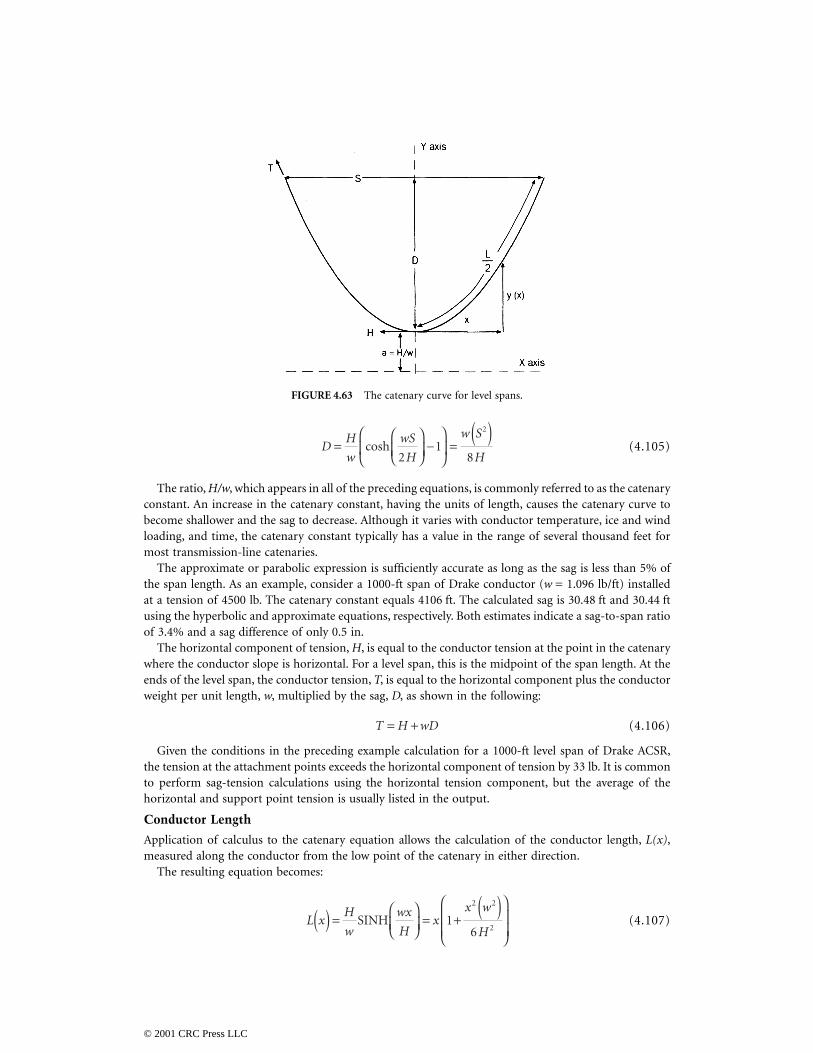
(4.105)

The ratio, H/w, which appears in all of the preceding equations, is commonly referred to as the catenaryconstant. An increase in the catenary constant, having the units of length, causes the catenary curve tobecome shallower and the sag to decrease. Although it varies with conductor temperature, ice and windloading, and time, the catenary constant typically has a value in the range of several thousand feet formost transmission-line catenaries.

The approximate or parabolic expression is sufficiently accurate as long as the sag is less than 5% ofthe span length. As an example, consider a 1000-ft span of Drake conductor (w = 1.096 lb/ft) installedat a tension of 4500 lb. The catenary constant equals 4106 ft. The calculated sag is 30.48 ft and 30.44 ftusing the hyperbolic and approximate equations, respectively. Both estimates indicate a sag-to-span ratioof 3.4% and a sag difference of only 0.5 in.

The horizontal component of tension, H, is equal to the conductor tension at the point in the catenarywhere the conductor slope is horizontal. For a level span, this is the midpoint of the span length. At theends of the level span, the conductor tension, T, is equal to the horizontal component plus the conductorweight per unit length, w, multiplied by the sag, D, as shown in the following:

(4.106)

Given the conditions in the preceding example calculation for a 1000-ft level span of Drake ACSR,the tension at the attachment points exceeds the horizontal component of tension by 33 lb. It is commonto perform sag-tension calculations using the horizontal tension component, but the average of thehorizontal and support point tension is usually listed in the output.

Conductor Length

Application of calculus to the catenary equation allows the calculation of the conductor length, L(x),measured along the conductor from the low point of the catenary in either direction.

The resulting equation becomes:

(4.107)

FIGURE 4.63 The catenary curve for level spans.

DH

w

wS

H

w S

H=

−

=

( )cosh

21

8

2

T H wD= +

L xH

w

wx

Hx

x w

H( ) =

= +

( )

SINH 16

2 2

2


For a level span, the conductor length corresponding to x = S/2 is half of the total conductor lengthand the total length, L, is:

(4.108)

The parabolic equation for conductor length can also be expressed as a function of sag, D, by substi-tution of the sag parabolic equation, giving:

(4.109)

Conductor Slack

The difference between the conductor length, L, and the span length, S, is called slack. The parabolicequations for slack may be found by combining the preceding parabolic equations for conductor length,L, and sag, D:

(4.110)

While slack has units of length, it is often expressed as the percentage of slack relative to the spanlength. Note that slack is related to the cube of span length for a given H/w ratio and to the square ofsag for a given span. For a series of spans having the same H/w ratio, the total slack is largely determinedby the longest spans. It is for this reason that the ruling span is nearly equal to the longest span ratherthan the average span in a series of suspension spans.

Equation (4.110) can be inverted to obtain a more interesting relationship showing the dependenceof sag, D, upon slack, L-S:

(4.111)

As can be seen from the preceding equation, small changes in slack typically yield large changes inconductor sag.

Inclined Spans

Inclined spans may be analyzed using essentially the same equations that were used for level spans. Thecatenary equation for the conductor height above the low point in the span is the same. However, thespan is considered to consist of two separate sections, one to the right of the low point and the other tothe left as shown in Fig. 4.64 (Winkelmann, 1959). The shape of the catenary relative to the low pointis unaffected by the difference in suspension point elevation (span inclination).

In each direction from the low point, the conductor elevation, y(x), relative to the low point is given by:

(4.112)

Note that x is considered positive in either direction from the low point.

LH

w

Sw

HS

S w

H=

= +

( )

2

21

24

2 2

2SINH

L SD

S= + 8

3

2

L S Sw

HD

S− =

=

3

2

2

2

24

8

3

DS L S

=−( )3

8

y xH

w

w

Hx

w x

H( ) =

−

=

( )cosh 1

2

2


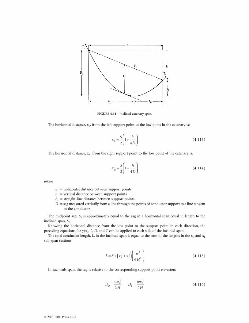
The horizontal distance, xL, from the left support point to the low point in the catenary is:

(4.113)

The horizontal distance, xR, from the right support point to the low point of the catenary is:

(4.114)

where

S = horizontal distance between support points.h = vertical distance between support points.S1 = straight-line distance between support points.D = sag measured vertically from a line through the points of conductor support to a line tangent

to the conductor.

The midpoint sag, D, is approximately equal to the sag in a horizontal span equal in length to theinclined span, S1.

Knowing the horizonal distance from the low point to the support point in each direction, thepreceding equations for y(x), L, D, and T can be applied to each side of the inclined span.

The total conductor length, L, in the inclined span is equal to the sum of the lengths in the xR and xL

sub-span sections:

(4.115)

In each sub-span, the sag is relative to the corresponding support point elevation:

(4.116)

FIGURE 4.64 Inclined catenary span.

xS h

DL = +

21

4

xS h

DR = −

21

4

L S x xw

HR L= + +( )

3 32

26

Dwx

HD

wx

HRR

LL= =

2 2

2 2


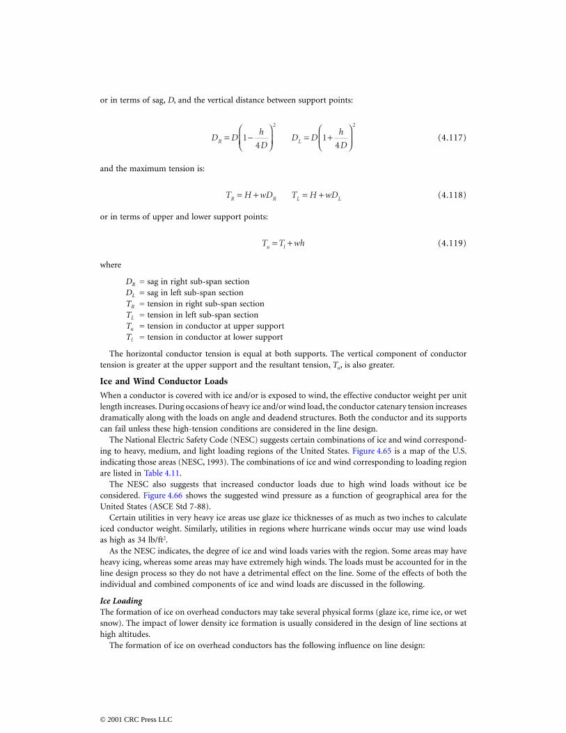
or in terms of sag, D, and the vertical distance between support points:

(4.117)

and the maximum tension is:

(4.118)

or in terms of upper and lower support points:

(4.119)

where

DR = sag in right sub-span sectionDL = sag in left sub-span sectionTR = tension in right sub-span sectionTL = tension in left sub-span sectionTu = tension in conductor at upper supportTl = tension in conductor at lower support

The horizontal conductor tension is equal at both supports. The vertical component of conductortension is greater at the upper support and the resultant tension, Tu, is also greater.

Ice and Wind Conductor Loads

When a conductor is covered with ice and/or is exposed to wind, the effective conductor weight per unitlength increases. During occasions of heavy ice and/or wind load, the conductor catenary tension increasesdramatically along with the loads on angle and deadend structures. Both the conductor and its supportscan fail unless these high-tension conditions are considered in the line design.

The National Electric Safety Code (NESC) suggests certain combinations of ice and wind correspond-ing to heavy, medium, and light loading regions of the United States. Figure 4.65 is a map of the U.S.indicating those areas (NESC, 1993). The combinations of ice and wind corresponding to loading regionare listed in Table 4.11.

The NESC also suggests that increased conductor loads due to high wind loads without ice beconsidered. Figure 4.66 shows the suggested wind pressure as a function of geographical area for theUnited States (ASCE Std 7-88).

Certain utilities in very heavy ice areas use glaze ice thicknesses of as much as two inches to calculateiced conductor weight. Similarly, utilities in regions where hurricane winds occur may use wind loadsas high as 34 lb/ft2.

As the NESC indicates, the degree of ice and wind loads varies with the region. Some areas may haveheavy icing, whereas some areas may have extremely high winds. The loads must be accounted for in theline design process so they do not have a detrimental effect on the line. Some of the effects of both theindividual and combined components of ice and wind loads are discussed in the following.

Ice LoadingThe formation of ice on overhead conductors may take several physical forms (glaze ice, rime ice, or wetsnow). The impact of lower density ice formation is usually considered in the design of line sections athigh altitudes.

The formation of ice on overhead conductors has the following influence on line design:

D Dh

DD D

h

DR L= −

= +

1

41

4

2 2

T H wD T H wDR R L L= + = +

T T whu l= +


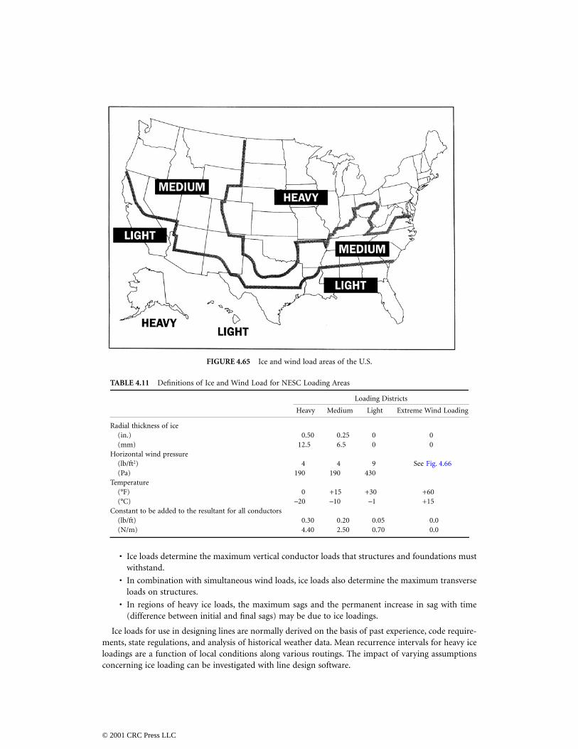
• Ice loads determine the maximum vertical conductor loads that structures and foundations mustwithstand.

• In combination with simultaneous wind loads, ice loads also determine the maximum transverseloads on structures.

• In regions of heavy ice loads, the maximum sags and the permanent increase in sag with time(difference between initial and final sags) may be due to ice loadings.

Ice loads for use in designing lines are normally derived on the basis of past experience, code require-ments, state regulations, and analysis of historical weather data. Mean recurrence intervals for heavy iceloadings are a function of local conditions along various routings. The impact of varying assumptionsconcerning ice loading can be investigated with line design software.

FIGURE 4.65 Ice and wind load areas of the U.S.

TABLE 4.11 Definitions of Ice and Wind Load for NESC Loading Areas

Loading Districts

Heavy Medium Light Extreme Wind Loading

Radial thickness of ice(in.)(mm)

0.5012.5

0.256.5

00

00

Horizontal wind pressure(lb/ft2)(Pa)

4190

4190

9430

See Fig. 4.66

Temperature(°F)(°C)

0–20

+15–10

+30–1

+60+15

Constant to be added to the resultant for all conductors(lb/ft)(N/m)

0.304.40

0.202.50

0.050.70

0.00.0


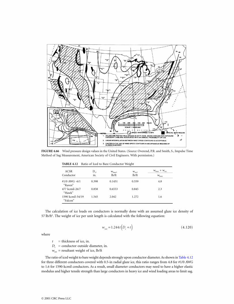
The calculation of ice loads on conductors is normally done with an assumed glaze ice density of57 lb/ft3. The weight of ice per unit length is calculated with the following equation:

(4.120)

where

t = thickness of ice, in.Dc = conductor outside diameter, in.wice = resultant weight of ice, lb/ft

The ratio of iced weight to bare weight depends strongly upon conductor diameter. As shown in Table 4.12for three different conductors covered with 0.5-in radial glaze ice, this ratio ranges from 4.8 for #1/0 AWGto 1.6 for 1590-kcmil conductors. As a result, small diameter conductors may need to have a higher elasticmodulus and higher tensile strength than large conductors in heavy ice and wind loading areas to limit sag.

FIGURE 4.66 Wind pressure design values in the United States. (Source: Overend, P.R. and Smith, S., Impulse TimeMethod of Sag Measurement, American Society of Civil Engineers. With permission.)

TABLE 4.12 Ratio of Iced to Bare Conductor Weight

ACSRConductor

Dc,in.

wbare,lb/ft

wice,lb/ft

wbare + wice

wbare

#1/0 AWG -6/1“Raven”

0.398 0.1451 0.559 4.8

477 kcmil-26/7“Hawk”

0.858 0.6553 0.845 2.3

1590 kcmil-54/19“Falcon”

1.545 2.042 1.272 1.6

w t D tcice = +( )1 244.


Wind LoadingWind loadings on overhead conductors influence line design in a number of ways:

• The maximum span between structures may be determined by the need for horizontal clearanceto edge of right-of-way during moderate winds.

• The maximum transverse loads for tangent and small angle suspension structures are oftendetermined by infrequent high wind-speed loadings.

• Permanent increases in conductor sag may be determined by wind loading in areas of light ice load.

Wind pressure load on conductors, Pw, is commonly specified in lb/ft2. The relationship between Pw

and wind velocity is given by the following equation:

(4.121)

where Vw = the wind speed in miles per hour.The wind load per unit length of conductor is equal to the wind pressure load, Pw, multiplied by the

conductor diameter (including radial ice of thickness t, if any), is given by the following equation:

(4.122)

Combined Ice and Wind LoadingIf the conductor weight is to include both ice and wind loading, the resultant magnitude of the loadsmust be determined vectorially. The weight of a conductor under both ice and wind loading is given bythe following equation:

(4.123)

where

wb = bare conductor weight per unit length, lb/ftwi = weight of ice per unit length, lb/ftww = wind load per unit length, lb/ftww± i = resultant of ice and wind loads, lb/ft

The NESC prescribes a safety factor, K, in pounds per foot, dependent upon loading district, to beadded to the resultant ice and wind loading when performing sag and tension calculations. Therefore,the total resultant conductor weight, w, is:

(4.124)

Conductor Tension Limits

The NESC recommends limits on the tension of bare overhead conductors as a percentage of theconductor’s rated breaking strength. The tension limits are: 60% under maximum ice and wind load,33.3% initial unloaded (when installed) at 60°F, and 25% final unloaded (after maximum loading hasoccurred) at 60°F. It is common, however, for lower unloaded tension limits to be used. Except in areasexperiencing severe ice loading, it is not unusual to find tension limits of 60% maximum, 25% unloadedinitial, and 15% unloaded final. This set of specifications could easily result in an actual maximum tensionon the order of only 35 to 40%, an initial tension of 20% and a final unloaded tension level of 15%. Inthis case, the 15% tension limit is said to govern.

P Vw w= ( )0 00252

.

W PD t

w w

c=+( )2

12

w w w Ww i b i w+ = +( ) + ( )2 2

w w Kw i= ++


Transmission-line conductors are normally not covered with ice, and winds on the conductor areusually much lower than those used in maximum load calculations. Under such everyday conditions,tension limits are specified to limit aeolian vibration to safe levels. Even with everyday lower tensionlevels of 15 to 20%, it is assumed that vibration control devices will be used in those sections of the linethat are subject to severe vibration. Aeolian vibration levels, and thus appropriate unloaded tension limits,vary with the type of conductor, the terrain, span length, and the use of dampers. Special conductors,such as ACSS, SDC, and VR, exhibit high self-damping properties and may be installed to the full codelimits, if desired.

Approximate Sag-Tension Calculations

Sag-tension calculations, using exacting equations, are usually performed with the aid of a computer;however, with certain simplifications, these calculations can be made with a handheld calculator. Thelatter approach allows greater insight into the calculation of sags and tensions than is possible withcomplex computer programs. Equations suitable for such calculations, as presented in the precedingsection, can be applied to the following example:

It is desired to calculate the sag and slack for a 600-ft level span of 795 kcmil-26/7 ACSR “Drake”conductor. The bare conductor weight per unit length, wb, is 1.094 lb/ft. The conductor is installed witha horizontal tension component, H, of 6300 lb, equal to 20% of its rated breaking strength of 31,500 lb.

By use of Eq. (4105), the sag for this level span is:

The length of the conductor between the support points is determined using Eq. (4.109):

Note that the conductor length depends solely on span and sag. It is not directly dependent onconductor tension, weight, or temperature. The conductor slack is the conductor length minus the spanlength; in this example, it is 0.27 ft (0.0826 m).

Sag Change with Thermal Elongation

ACSR and AAC conductors elongate with increasing conductor temperature. The rate of linear thermalexpansion for the composite ACSR conductor is less than that of the AAC conductor because the steelstrands in the ACSR elongate at approximately half the rate of aluminum. The effective linear thermalexpansion coefficient of a non-homogenous conductor, such as Drake ACSR, may be found from thefollowing equations (Fink and Beatty):

(4.125)

(4.126)

where

D =( )

( ) = ( )1 094 600

8 63007 81 2 38

2.. .ft m

L = +( )( ) = ( )600

8 7 81

3 600600 27 182 96

2

.. .ft m

E EA

AE

A

AAS ALAL

TOTAL

STST

TOTAL

=

+

α α αASAL

AS

AL

TOTAL

STST

AS

ST

TOTAL

E

E

A

A

E

E

A

A=

+

AL


EAL = Elastic modulus of aluminum, psiEST = Elastic modulus of steel, psiEAS = Elastic modulus of aluminum-steel composite, psiAAL = Area of aluminum strands, square unitsAST = Area of steel strands, square unitsATOTAL = Total cross-sectional area, square unitsαAL = Aluminum coefficient of linear thermal expansion, per °FαST = Steel coefficient of thermal elongation, per °FαAS = Composite aluminum-steel coefficient of thermal elongation, per °F

The elastic moduli for solid aluminum wire is 10 million psi and for steel wire is 30 million psi. Theelastic moduli for stranded wire is reduced. The modulus for stranded aluminum is assumed to be8.6 million psi for all strandings. The moduli for the steel core of ACSR conductors varies with strandingas follows:

• 27.5 × 106 for single-strand core

• 27.0 × 106 for 7-strand core

• 26.5 × 106 for 19-strand core

Using elastic moduli of 8.6 and 27.0 million psi for aluminum and steel, respectively, the elasticmodulus for Drake ACSR is:

and the coefficient of linear thermal expansion is:

If the conductor temperature changes from a reference temperature, TREF , to another temperature, T,the conductor length, L, changes in proportion to the product of the conductor’s effective thermalelongation coefficient, αAS, and the change in temperature, T – TREF , as shown below:

(4.127)

For example, if the temperature of the Drake conductor in the preceding example increases from 60°F(15°C) to 167°F (75°C), then the length at 60°F increases by 0.68 ft (0.21 m) from 600.27 ft (182.96 m)to 600.95 ft (183.17 m):

Ignoring for the moment any change in length due to change in tension, the sag at 167°F (75°C) maybe calculated for the conductor length of 600.95 ft (183.17 m) using Eq. (4.111):

EAS = ×( )

+ ×( )

= ×8 6 10

0 6247

0 726427 0 10

0 1017

0 726411 2 106 6 6.

.

..

.

.. psi

αAS = × ××

+ × ×

×

= × °

− −

−

12 8 108 6 10

11 2 10

0 6247

0 72646 4 10

27 0 10

11 2 10

0 1017

0 7264

10 6 10

66

6

66

6

6

..

.

.

..

.

.

.

.

. F

L L T TT T AS REFREF= + −( )( )1 α

LF167

6600 27 1 10 6 10 167 60 600 95°( )−= + ×( ) −( )( ) =. . . ft

D =( )( )

=3 600 0 95

814 62

.. ft


Using a rearrangement of Eq. (4.105), this increased sag is found to correspond to a decreased tension of:

If the conductor were inextensible, that is, if it had an infinite modulus of elasticity, then these valuesof sag and tension for a conductor temperature of 167°F would be correct. For any real conductor,however, the elastic modulus of the conductor is finite and changes in tension do change the conductorlength. Use of the preceding calculation, therefore, will overstate the increase in sag.

Sag Change Due to Combined Thermal and Elastic Effects

With moduli of elasticity around the 8.6 million psi level, typical bare aluminum and ACSR conductorselongate about 0.01% for every 1000 psi change in tension. In the preceding example, the increase intemperature caused an increase in length and sag and a decrease in tension, but the effect of tensionchange on length was ignored.

As discussed later, concentric-lay stranded conductors, particularly non-homogenous conductors suchas ACSR, are not inextensible. Rather, they exhibit quite complex elastic and plastic behavior. Initialloading of conductors results in elongation behavior substantially different from that caused by loadingmany years later. Also, high tension levels caused by heavy ice and wind loads cause a permanent increasein conductor length, affecting subsequent elongation under various conditions.

Accounting for such complex stress-strain behavior usually requires a sophisticated, computer-aidedapproach. For illustration purposes, however, the effect of permanent elongation of the conductor on sagand tension calculations will be ignored and a simplified elastic conductor assumed. This idealized conductoris assumed to elongate linearly with load and to undergo no permanent increase in length regardless ofloading or temperature. For such a conductor, the relationship between tension and length is as follows:

(4.128)

where

LH = Length of conductor under horizontal tension HLHREF

= Length of conductor under horizontal reference tension HREF

EC = Elastic modulus of elasticity of the conductor, psiA = Cross-sectional area, in.2

In calculating sag and tension for extensible conductors, it is useful to add a step to the precedingcalculation of sag and tension for elevated temperature. This added step allows a separation of thermalelongation and elastic elongation effects, and involves the calculation of a zero tension length, ZTL, atthe conductor temperature of interest, Tcdr .

This ZTL(Tcdr) is the conductor length attained if the conductor is taken down from its supports andlaid on the ground with no tension. By reducing the initial tension in the conductor to zero, the elasticelongation is also reduced to zero, shortening the conductor. It is possible, then, for the zero tensionlength to be less than the span length.

Consider the preceding example for Drake ACSR in a 600-ft level span. The initial conductor temper-ature is 60°F, the conductor length is 600.27 ft, and EAS is calculated to be 11.2 million psi. UsingEq. (4.128), the reduction of the initial tension from 6300 lb to zero yields a ZTL (60°F) of:

Hw S

D=

( )=

( )( ) =

2 2

8

1 094 600

8 14 623367

.

.lb

L LH H

E AH HREF

CREF

= + −

1

ZTLF60 6

600 27 10 6300

11 2 10 0 7264599 81°( ) = + −

×( )

=.. .

. ft


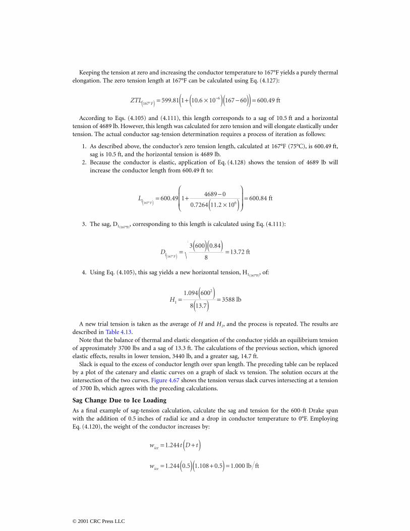
Keeping the tension at zero and increasing the conductor temperature to 167°F yields a purely thermalelongation. The zero tension length at 167°F can be calculated using Eq. (4.127):

According to Eqs. (4.105) and (4.111), this length corresponds to a sag of 10.5 ft and a horizontaltension of 4689 lb. However, this length was calculated for zero tension and will elongate elastically undertension. The actual conductor sag-tension determination requires a process of iteration as follows:

1. As described above, the conductor’s zero tension length, calculated at 167°F (75°C), is 600.49 ft,sag is 10.5 ft, and the horizontal tension is 4689 lb.

2. Because the conductor is elastic, application of Eq. (4.128) shows the tension of 4689 lb willincrease the conductor length from 600.49 ft to:

3. The sag, D1(167°F), corresponding to this length is calculated using Eq. (4.111):

4. Using Eq. (4.105), this sag yields a new horizontal tension, H1(167°F), of:

A new trial tension is taken as the average of H and H1, and the process is repeated. The results aredescribed in Table 4.13.

Note that the balance of thermal and elastic elongation of the conductor yields an equilibrium tensionof approximately 3700 lbs and a sag of 13.3 ft. The calculations of the previous section, which ignoredelastic effects, results in lower tension, 3440 lb, and a greater sag, 14.7 ft.

Slack is equal to the excess of conductor length over span length. The preceding table can be replacedby a plot of the catenary and elastic curves on a graph of slack vs tension. The solution occurs at theintersection of the two curves. Figure 4.67 shows the tension versus slack curves intersecting at a tensionof 3700 lb, which agrees with the preceding calculations.

Sag Change Due to Ice Loading

As a final example of sag-tension calculation, calculate the sag and tension for the 600-ft Drake spanwith the addition of 0.5 inches of radial ice and a drop in conductor temperature to 0°F. EmployingEq. (4.120), the weight of the conductor increases by:

ZTLF167

6599 81 1 10 6 10 167 60 600 49°( )−= + ×( ) −( )( ) =. . . ft

Ll F167600 49 1

4689 0

0 7264 11 2 10600 84

6°( ) = + −×( )

=.. .

. ft

Dl F167

3 600 0 84

813 72

°( ) =( )( )

=.

. ft

H1

21 094 600

8 13 73588=

( )( ) =

.

.lb

w t D tice = +( )1 244.

wice = ( ) +( ) =1 244 0 5 1 108 0 5 1 000. . . . . lb ft


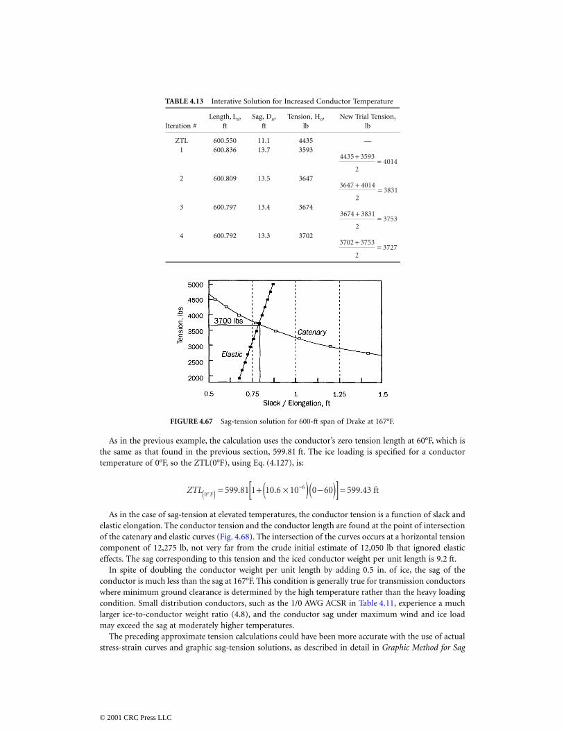
As in the previous example, the calculation uses the conductor’s zero tension length at 60°F, which isthe same as that found in the previous section, 599.81 ft. The ice loading is specified for a conductortemperature of 0°F, so the ZTL(0°F), using Eq. (4.127), is:

As in the case of sag-tension at elevated temperatures, the conductor tension is a function of slack andelastic elongation. The conductor tension and the conductor length are found at the point of intersectionof the catenary and elastic curves (Fig. 4.68). The intersection of the curves occurs at a horizontal tensioncomponent of 12,275 lb, not very far from the crude initial estimate of 12,050 lb that ignored elasticeffects. The sag corresponding to this tension and the iced conductor weight per unit length is 9.2 ft.

In spite of doubling the conductor weight per unit length by adding 0.5 in. of ice, the sag of theconductor is much less than the sag at 167°F. This condition is generally true for transmission conductorswhere minimum ground clearance is determined by the high temperature rather than the heavy loadingcondition. Small distribution conductors, such as the 1/0 AWG ACSR in Table 4.11, experience a muchlarger ice-to-conductor weight ratio (4.8), and the conductor sag under maximum wind and ice loadmay exceed the sag at moderately higher temperatures.

The preceding approximate tension calculations could have been more accurate with the use of actualstress-strain curves and graphic sag-tension solutions, as described in detail in Graphic Method for Sag

TABLE 4.13 Interative Solution for Increased Conductor Temperature

Iteration #Length, Ln,

ftSag, Dn,

ftTension, Hn,

lb New Trial Tension,

lb

ZTL 600.550 11.1 4435 —1 600.836 13.7 3593

2 600.809 13.5 3647

3 600.797 13.4 3674

4 600.792 13.3 3702

FIGURE 4.67 Sag-tension solution for 600-ft span of Drake at 167°F.

4435 3593

24014

+=

3647 4014

23831

+=

3674 3831

23753

+=

3702 3753

23727

+=

ZTLF0

6599 81 1 10 6 10 0 60 599 43°( )−= + ×( ) −( )[ ] =. . . ft


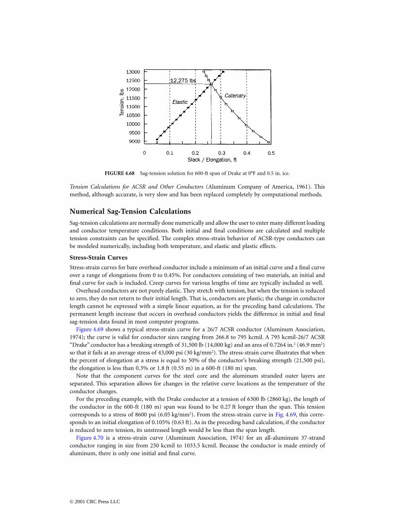
Tension Calculations for ACSR and Other Conductors (Aluminum Company of America, 1961). Thismethod, although accurate, is very slow and has been replaced completely by computational methods.

Numerical Sag-Tension Calculations

Sag-tension calculations are normally done numerically and allow the user to enter many different loadingand conductor temperature conditions. Both initial and final conditions are calculated and multipletension constraints can be specified. The complex stress-strain behavior of ACSR-type conductors canbe modeled numerically, including both temperature, and elastic and plastic effects.

Stress-Strain Curves

Stress-strain curves for bare overhead conductor include a minimum of an initial curve and a final curveover a range of elongations from 0 to 0.45%. For conductors consisting of two materials, an initial andfinal curve for each is included. Creep curves for various lengths of time are typically included as well.

Overhead conductors are not purely elastic. They stretch with tension, but when the tension is reducedto zero, they do not return to their initial length. That is, conductors are plastic; the change in conductorlength cannot be expressed with a simple linear equation, as for the preceding hand calculations. Thepermanent length increase that occurs in overhead conductors yields the difference in initial and finalsag-tension data found in most computer programs.

Figure 4.69 shows a typical stress-strain curve for a 26/7 ACSR conductor (Aluminum Association,1974); the curve is valid for conductor sizes ranging from 266.8 to 795 kcmil. A 795 kcmil-26/7 ACSR“Drake” conductor has a breaking strength of 31,500 lb (14,000 kg) and an area of 0.7264 in.2 (46.9 mm2)so that it fails at an average stress of 43,000 psi (30 kg/mm2). The stress-strain curve illustrates that whenthe percent of elongation at a stress is equal to 50% of the conductor’s breaking strength (21,500 psi),the elongation is less than 0.3% or 1.8 ft (0.55 m) in a 600-ft (180 m) span.

Note that the component curves for the steel core and the aluminum stranded outer layers areseparated. This separation allows for changes in the relative curve locations as the temperature of theconductor changes.

For the preceding example, with the Drake conductor at a tension of 6300 lb (2860 kg), the length ofthe conductor in the 600-ft (180 m) span was found to be 0.27 ft longer than the span. This tensioncorresponds to a stress of 8600 psi (6.05 kg/mm2). From the stress-strain curve in Fig. 4.69, this corre-sponds to an initial elongation of 0.105% (0.63 ft). As in the preceding hand calculation, if the conductoris reduced to zero tension, its unstressed length would be less than the span length.

Figure 4.70 is a stress-strain curve (Aluminum Association, 1974) for an all-aluminum 37-strandconductor ranging in size from 250 kcmil to 1033.5 kcmil. Because the conductor is made entirely ofaluminum, there is only one initial and final curve.

FIGURE 4.68 Sag-tension solution for 600-ft span of Drake at 0°F and 0.5 in. ice.


4 Transmission System - Electrical...

Documents

Transcript of 4 Transmission System - Electrical...