Migration of a Complete 3D Poisson Solver g pfrom Optimized Fortran77 to GPU

Huynh Phung HuynhShyh‐hao Kuo

Rick Siow Mong Goh Le Duc VinhLe Duc VinhTerence Hung

A*STAR I i f Hi h P f C i (IHPC)A*STAR Institute of High Performance Computing (IHPC)Singapore

OutlineOutline

3D P i S l• 3D Poisson Solver

• Algorithm FlowAlgorithm Flow

• Mapping to GPUpp g

• Experimental Results

• Conclusions and Future Work

3D Poisson Solver3D Poisson Solver

222 ),,(),,(222 zyxfzyxzyx

Wide range applications of Poisson Solver: Fl id D i

Fluid Dynamic Solar Magnetostatics Electrostatics Electrostatics Mechanical Engineer Theoretical physics Theoretical physics …

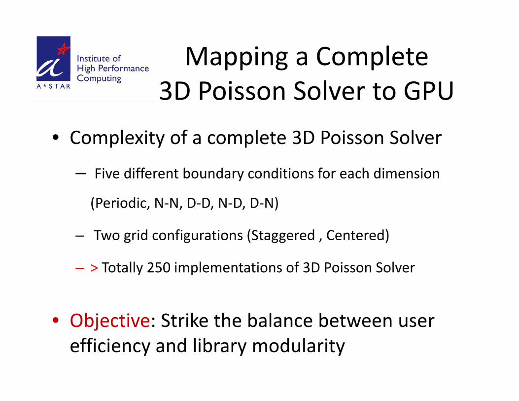
Mapping a Complete 3D Poisson Solver to GPU

• Complexity of a complete 3D Poisson Solver

– Five different boundary conditions for each dimensionFive different boundary conditions for each dimension 

(Periodic, N‐N, D‐D, N‐D, D‐N)

– Two grid configurations (Staggered , Centered)

– > Totally 250 implementations of 3D Poisson Solver

• Objective: Strike the balance between user Object e St e t e ba a ce bet ee useefficiency and library modularity

OutlineOutline

3D P i S l• 3D Poisson Solver

• Algorithm FlowAlgorithm Flow

• Mapping to GPUpp g

• Experimental Results

• Conclusions and Future Work

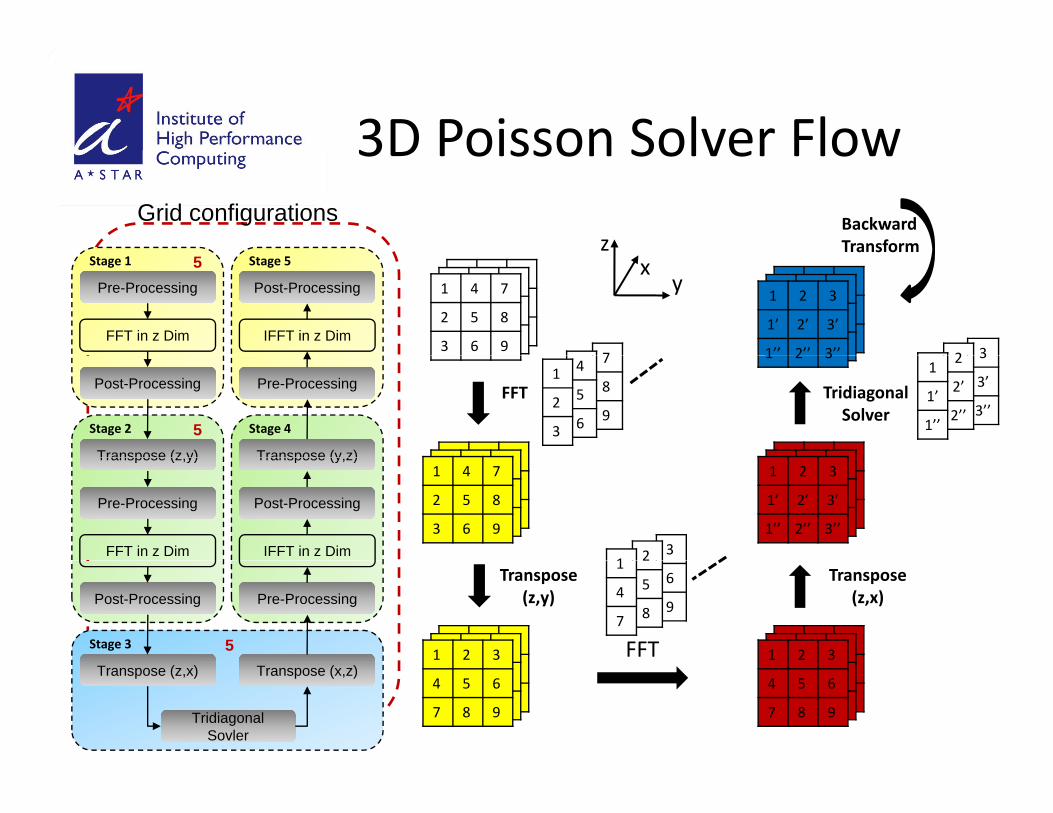
3D Poisson Solver FlowGrid configurations

3D Poisson Solver Flow  

zBackward Transform

7

yx

1 4 7

2 5 8

3 6 9

1 2 3

1’    2’ 3’

1’’ 2’’ 3’’ 32

Pre-Processing

FFT in z Dim

Post-Processing

IFFT in z Dim

Stage 1 Stage 55

7

8

9

4

5

6

1

2

3

FFT Tridiagonal Solver

1 2 3 3

3’

3’’

2

2’

2’’

1

1’

1’’

Post-Processing

Transpose (z y)

Pre-Processing

Transpose (y z)

Stage 2 Stage 45

1 4 7

2 5 8

3 6 9321

1 2 3

1’    2’ 3’

1’’ 2’’ 3’’

Transpose (z,y)

Pre-Processing

FFT in z Dim

Transpose (y,z)

Post-Processing

IFFT in z Dim

FFT

Transpose(z,x)

1 2 3

6

9

2

5

8

1

4

7

1 2 3

Transpose(z,y)Post-Processing Pre-Processing

Stage 3 5

4 5 6

7 8 9

4 5 6

7 8 9

Transpose (z,x)

TridiagonalSovler

Transpose (x,z)

OutlineOutline

3D P i S l• 3D Poisson Solver

• Algorithm FlowAlgorithm Flow

• Mapping to GPUpp g

• Experimental Results

• Conclusions and Future Work

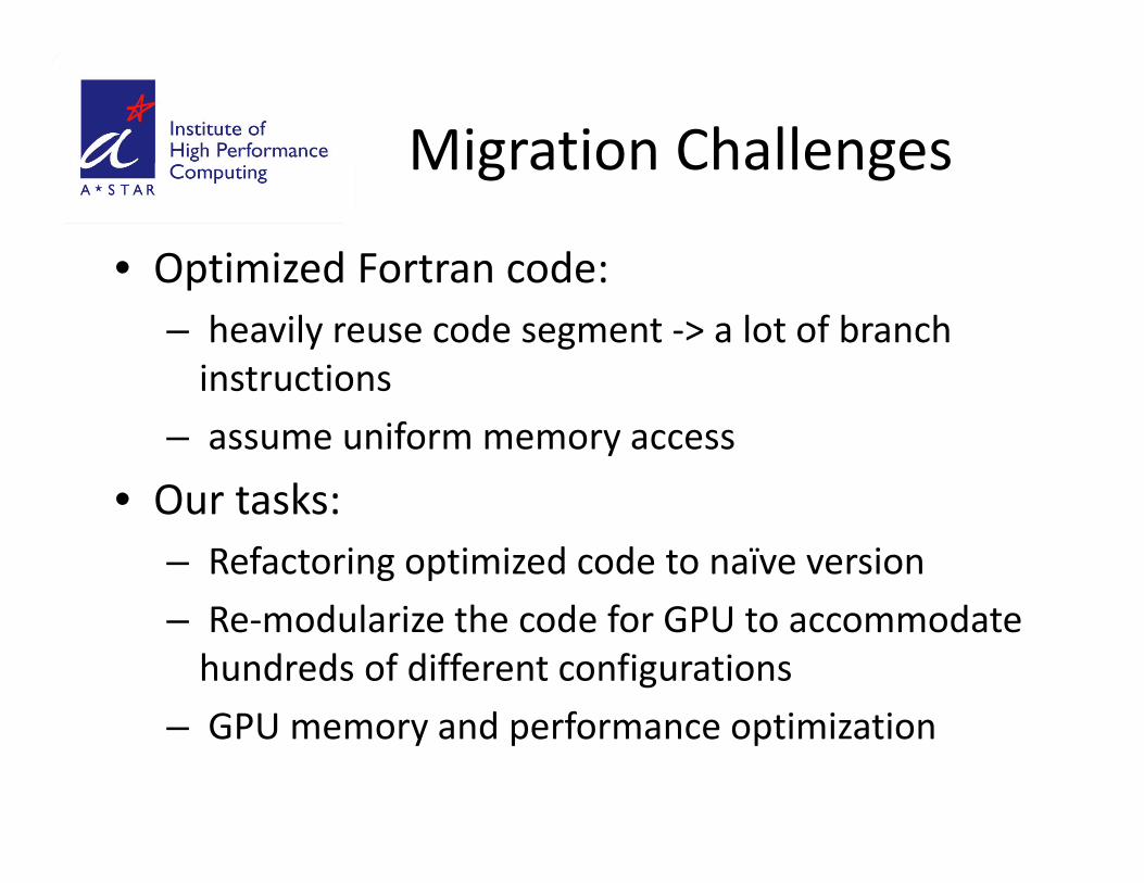
Migration ChallengesMigration Challenges

• Optimized Fortran code:Optimized Fortran code:– heavily reuse code segment ‐> a lot of branch instructionsinstructions

– assume uniform memory access

• Our tasks:• Our tasks:– Refactoring optimized code to naïve version

R d l i th d f GPU t d t– Re‐modularize the code for GPU to accommodate hundreds of different configurations

GPU memory and performance optimization– GPU memory and performance optimization

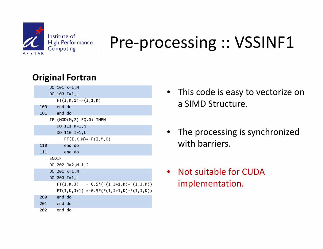
Pre‐processing :: VSSINF1Pre processing :: VSSINF1

Original FortranDO 101 K=1,NDO 100 I=1,L

FT(I,K,1)=F(I,1,K)100    end do

• This code is easy to vectorize on a SIMD Structure.

Original Fortran

101    end doIF (MOD(M,2).EQ.0) THEN

DO 111 K=1,NDO 110 I=1,L

FT(I,K,M)=‐F(I,M,K)• The processing is synchronized 

h bFT(I,K,M) F(I,M,K)

110       end do111       end do

ENDIFDO 202 J=2,M‐1,2DO 201 K=1 N

with barriers.

• Not suitable for CUDADO 201 K=1,NDO 200 I=1,L

FT(I,K,J)   = 0.5*(F(I,J+1,K)‐F(I,J,K))FT(I,K,J+1) =‐0.5*(F(I,J+1,K)+F(I,J,K))

200    end do201    end do

• Not suitable for CUDA implementation.

201    end do202    end do

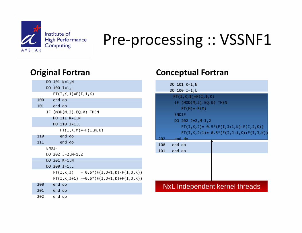
Pre‐processing :: VSSNF1Pre processing :: VSSNF1

Original Fortran Conceptual FortranOriginal FortranDO 101 K=1,NDO 100 I=1,L

FT(I,K,1)=F(I,1,K)100    end do

Conceptual FortranDO 101 K=1,N  DO 100 I=1,L  FT(I,K,1)=F(I,1,K)IF (MOD(M 2) EQ 0) THEN

101    end doIF (MOD(M,2).EQ.0) THEN

DO 111 K=1,NDO 110 I=1,L

FT(I,K,M)=‐F(I,M,K)

IF (MOD(M,2).EQ.0) THENFT(M)=‐F(M)

ENDIFDO 202 J=2,M‐1,2

FT(I,K,J)= 0.5*(F(I,J+1,K)‐F(I,J,K))( ) *( ( ) ( ))

FT(I,K,M) F(I,M,K)110       end do111       end do

ENDIFDO 202 J=2,M‐1,2DO 201 K=1 N

FT(I,K,J+1)=‐0.5*(F(I,J+1,K)+F(I,J,K))202    end do100   end do101   end do

DO 201 K=1,NDO 200 I=1,L

FT(I,K,J)   = 0.5*(F(I,J+1,K)‐F(I,J,K))FT(I,K,J+1) =‐0.5*(F(I,J+1,K)+F(I,J,K))

200    end do201    end do

NxL Independent kernel threads201    end do202    end do

p

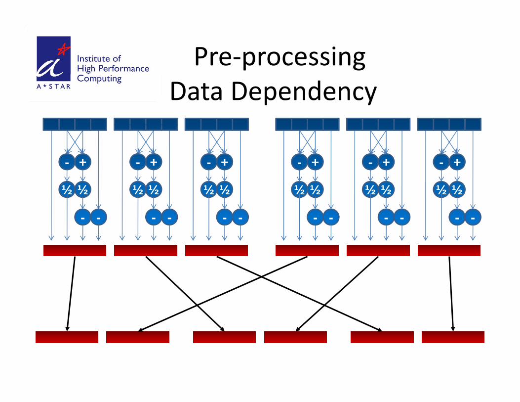
Pre‐processingData Dependency

+- +- +- +- +- +-

-

½ ½

- -

½ ½

- -

½ ½

- -

½ ½

- -

½ ½

- -

½ ½

-

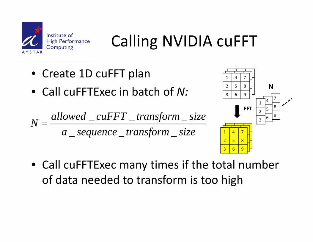
Calling NVIDIA cuFFTCalling NVIDIA cuFFT

• Create 1D cuFFT planCreate 1D cuFFT plan

• Call cuFFTExec in batch of N:7

8

1 4 7

2 5 8

3 6 941

N

sizetransformsequenceasizetransformcuFFTallowedN ___

8

9

1 4 7

5

62

3

FFT

• Call cuFFTExec many times if the total number

fq ___2 5 8

3 6 9

Call cuFFTExec many times if the total number of data needed to transform is too high

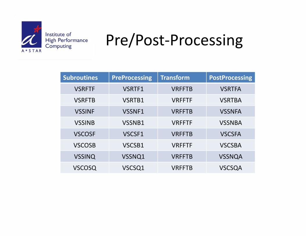
Pre/Post‐ProcessingPre/Post Processing

Subroutines PreProcessing Transform PostProcessing

VSRFTF VSRTF1 VRFFTB VSRTFA

VSRFTB VSRTB1 VRFFTF VSRTBA

VSSINF VSSNF1 VRFFTB VSSNFA

VSSINB VSSNB1 VRFFTF VSSNBA

VSCOSF VSCSF1 VRFFTB VSCSFAVSCOSF VSCSF1 VRFFTB VSCSFA

VSCOSB VSCSB1 VRFFTF VSCSBA

VSSINQ VSSNQ1 VRFFTB VSSNQA

VSCOSQ VSCSQ1 VRFFTB VSCSQA

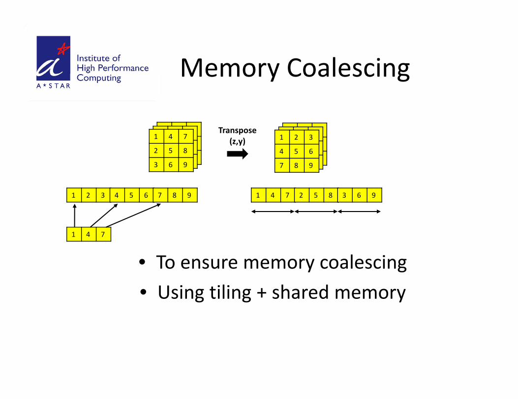
Memory CoalescingMemory Coalescing

1 4 7

2 5 8

3 6 9

1 2 3

4 5 6

7 8 9

Transpose(z,y)

1 2 3 4 5 6 7 8 9 1 4 7 2 5 8 3 6 9

• To ensure memory coalescing

1 4 7

• Using tiling + shared memory

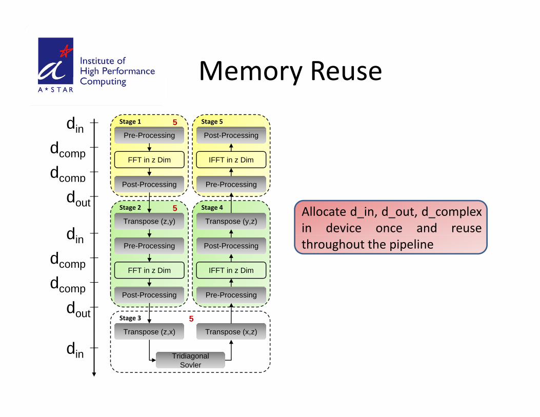
Memory ReuseMemory Reuse

Stage 1 Stage 55dinPre-Processing

FFT in z Dim

P t P i

Post-Processing

IFFT in z Dim

P P i

in

dcomp

dcomp

Allocate d_in, d_out, d_complexin device once and reuse

Post-Processing

Transpose (z,y)

Pre-Processing

Transpose (y,z)

Stage 2 Stage 45dout

dthroughout the pipelinePre-Processing

FFT in z Dim

Post-Processing

IFFT in z Dim

din

dcomp

dcompPost-Processing

Transpose (z,x)

Pre-Processing

Transpose (x,z)

Stage 3 5

dcomp

dout

TridiagonalSovler

din

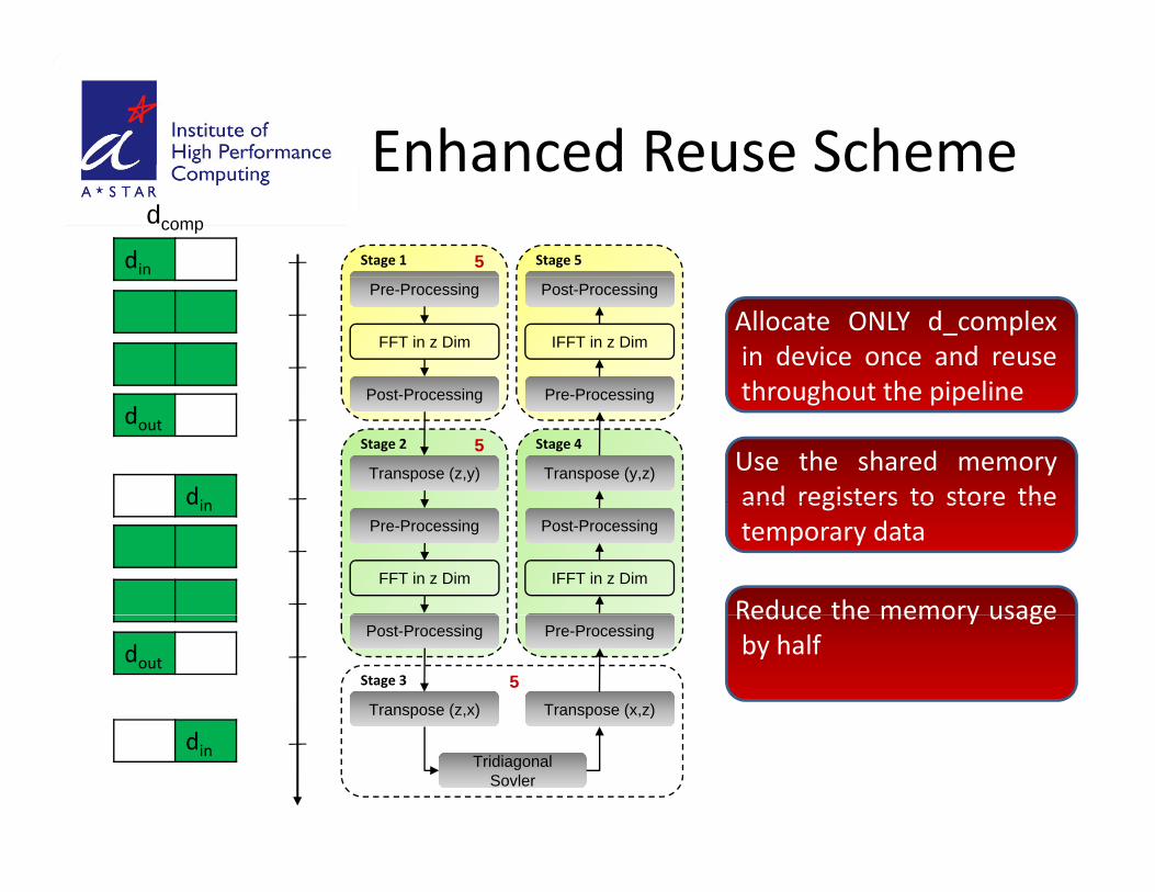
Enhanced Reuse SchemeEnhanced Reuse Scheme

Stage 1 Stage 55din

dcomp

Allocate ONLY d_complexin device once and reusethroughout the pipeline

Pre-Processing

FFT in z Dim

P t P i

Post-Processing

IFFT in z Dim

P P i throughout the pipelinePost-Processing

Transpose (z,y)

Pre-Processing

Transpose (y,z)

Stage 2 Stage 45dout

di

Use the shared memoryand registers to store the

Pre-Processing

FFT in z Dim

Post-Processing

IFFT in z Dim

din and registers to store thetemporary data

Reduce the memory usagePost-Processing

Transpose (z,x)

Pre-Processing

Transpose (x,z)

Stage 3 5dout

Reduce the memory usageby half

TridiagonalSovler

din

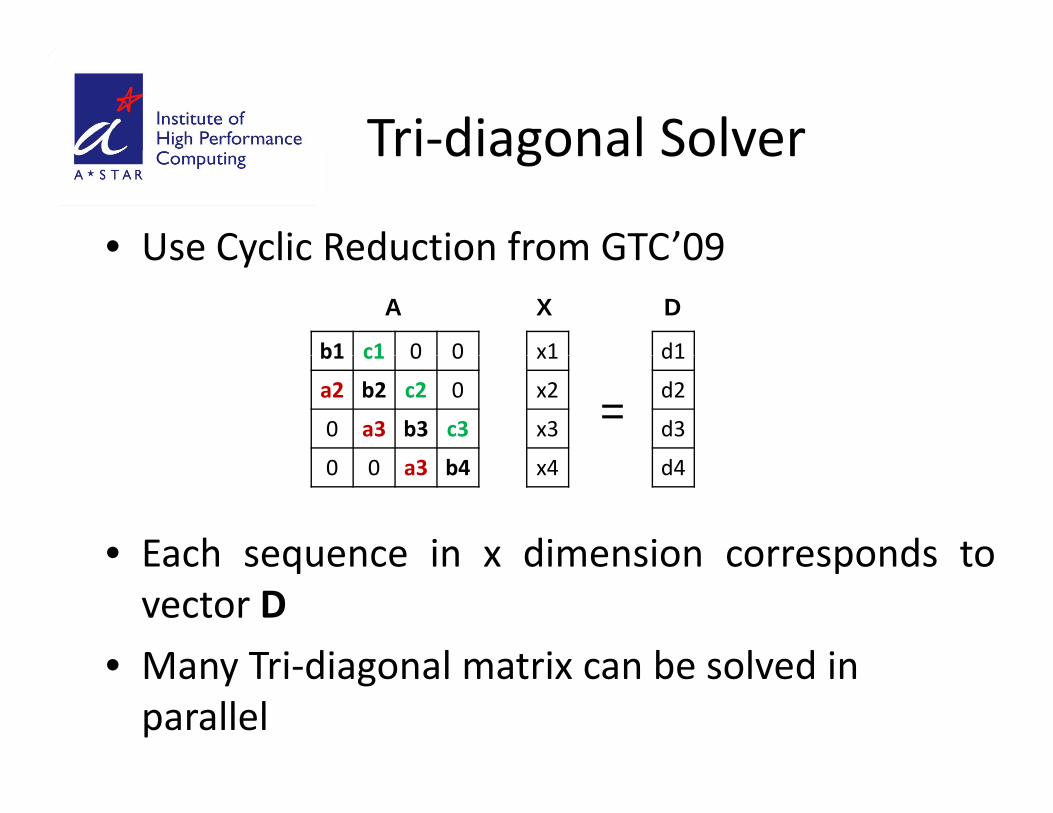
Tri‐diagonal SolverTri diagonal Solver

• Use Cyclic Reduction from GTC’09Use Cyclic Reduction from GTC 09

b1 c1 0 0 x1 d1

A X D

b1 c1 0 0

a2 b2 c2 0

0 a3 b3 c3

x1

x2

x3 =d1

d2

d3

• Each sequence in x dimension corresponds to

0 0 a3 b4 x4 d4

Each sequence in x dimension corresponds tovector D

• Many Tri diagonal matrix can be solved in• Many Tri‐diagonal matrix can be solved in parallel

OutlineOutline

3D P i S l• 3D Poisson Solver

• Algorithm FlowAlgorithm Flow

• Mapping to GPUpp g

• Experimental Results

• Conclusions and Future Work

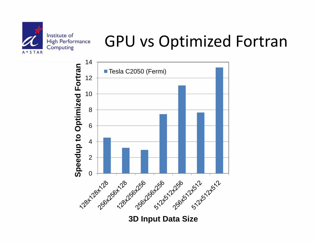
GPU vs Optimized FortranGPU vs Optimized Fortran 

12

14

ran

Tesla C2050 (Fermi)

10

12ze

d Fo

rt

6

8

o O

ptim

iz

2

4

peed

up to

0Sp

3D Input Data Size

Conclusions & Future WorkConclusions & Future Work

• Provide a generic Poisson Solver library interfaceProvide a generic Poisson Solver library interface

i G i h 3 i f h• Fermi GPU version has up to 13 times faster than optimized Fortran77 version (8‐core Intel Xeon(R) 3 0 Gh )3.0 Ghz) 

• Implement Multiple‐GPU version

Thank you!Thank you!

• Questions?Questions?