Improvements to the APBS biomolecular solvationsoftware suite

Elizabeth Jurrus?, Dave Engel?, Keith Star?, Kyle Monson?, Juan Brandi?,Lisa E. Felberg†, David H. Brookes†, Leighton Wilson‡, Jiahui Chen§,

Karina Liles?, Minju Chun?, Peter Li?, Todd Dolinsky‖, Robert Konecny∆,David R. KoesB, Jens Erik Nielsen¶, Teresa Head-Gordon†, Weihua Geng§,

Robert Krasny‡, Guo-Wei Wei∇, Michael J. Holst∆,J. Andrew McCammon∆, and Nathan A. BakerC

?Pacific Northwest National Laboratory†University of California, Berkeley

‡University of Michigan§Southern Methodist University

‖FoodLogiQBUniversity of Pittsburgh

¶Protein Engineering, Novozymes A/S∇Michigan State University

∆University of California San DiegoCTo whom correspondence should be addressed. Advanced Computing,

Mathematics, and Data Division; Pacific Northwest National Laboratory;Richland, WA 99352, USA. Division of Applied Mathematics; Brown

University; Providence, RI 02912, USA. Email: nathan.baker@pnnl.gov

July 4, 2017

arX

iv:1

707.

0002

7v1

[q-

bio.

BM

] 3

0 Ju

n 20

17

Abstract

The Adaptive Poisson-Boltzmann Solver (APBS) software was developed to solve the equa-tions of continuum electrostatics for large biomolecular assemblages that has provided impactin the study of a broad range of chemical, biological, and biomedical applications. APBSaddresses three key technology challenges for understanding solvation and electrostatics inbiomedical applications: accurate and efficient models for biomolecular solvation and elec-trostatics, robust and scalable software for applying those theories to biomolecular systems,and mechanisms for sharing and analyzing biomolecular electrostatics data in the scientificcommunity. To address new research applications and advancing computational capabilities,we have continually updated APBS and its suite of accompanying software since its releasein 2001. In this manuscript, we discuss the models and capabilities that have recently beenimplemented within the APBS software package including: a Poisson-Boltzmann analyticaland a semi-analytical solver, an optimized boundary element solver, a geometry-based ge-ometric flow solvation model, a graph theory based algorithm for determining pKa values,and an improved web-based visualization tool for viewing electrostatics.

1 Introduction

Robust models of electrostatic interactions are important for understanding early molecularrecognition events where long-ranged intermolecular interactions and the effects of solvationon biomolecular processes dominate. While explicit electrostatic models that treat the so-lute and solvent in atomic detail are common, these approaches generally require extensiveequilibration and sampling to converge properties of interest in the statistical ensemble ofinterest. Coarse-graining approaches that integrate out important, but largely uninterestingdegrees of freedom, sacrifice numerical precision in favor of robust but qualitative accuracyand efficiency by eliminating the need for sampling and equilibration associated with explicitsolute and solvent models.

While there is a choice among several implicit solvation models [1–6], one of the mostpopular implicit solvent models for biomolecules is based on the Poisson-Boltzmann (PB)equation [7–9]. The PB equation provides a global solution for the electrostatic potential(φ) within and around a biomolecule by solving the partial differential equation

−∇ · ε∇φ−M∑i

ciqie−β(qiφ+Vi) = ρ. (1)

The solvent is described by the bulk solvent dielectric constant εs as well as the propertiesof i = 1, . . . ,M mobile ion species, described by their charges qi, concentrations ci, andsteric ion-solute interaction potential Vi. The biomolecular structure is incorporated into theequation through Vi, a dielectric coefficient function ε, and a charge distribution function ρ.The dielectric ε is often set to a constant value εm in the interior of the molecule and variessharply across the molecular boundary to the value εs which describes the bulk solvent.The shape of the boundary is determined by the size and location of the solute atoms aswell as model-specific parameters such as a characteristic solvent molecule size [10]. Thecharge distribution ρ is usually a sum of Dirac delta distributions which are located atatom centers. Finally, β = (kT )−1 is the inverse thermal energy where k is the Boltzmannconstant and T is the temperature. The potential φ can be used in a variety of applications,including visualization, other structural analyses, diffusion simulations, and a number ofother calculations that require global electrostatic properties. The PB theory is approximateand, as a result, has several well-known limitations which can affect its accuracy, particularlyfor strongly charged systems or high salt concentrations [7, 11]. Despite these limitations, PBmethods are still very important and popular for biomolecular structural analysis, modeling,and simulation.

Several software packages have been developed that solve the Poisson-Boltzmann equa-tions to evaluate energies, potentials, and other solvation properties. The most significant(based on user base and citations) of these include CHARMM [12], AMBER [13], DelPhi [14],Jaguar [15], Zap [16], MIBPB [17], and APBS [18]. However the APBS and associated soft-ware package PDB2PQR has served a large community of ∼27,000 users by creating webservers linked from the APBS website [19] that support preparation of biomolecular struc-tures (see Section 2) and a fast finite-difference solution of the Poisson-Boltzmann equation(see Section 3.1) that are further augmented with a set of analysis tools. Most APBS elec-trostatics calculations follow the general workflow outlined in Figure 1. An even broader

1

Typical APBS & PDB2PQR user workflow

PDB2PQR onlyUserAPBS &

PDB2PQRAPBS only

Start

Upload a structure or

specify ID

Repair heavy atoms

Assign titration

states

End

Add hydrogens

Assign charge & radius

parameters

Web-based visualization

Offline visualization

& analysis

Calculate electrostatic properties

Figure 1: Workflow for biomolecular electrostatics calculations using the APBS-PDB2PQRsoftware suite. This workflow is supported by the APBS tool suite with specific support byPDB2PQR for preparing biomolecular structures (see Section 2) and support by APBS forperforming electrostatics calculations (see Section 3).

range of features and more flexible configuration is available when APBS and PDB2PQRare run from the command line on Linux, Mac, and Windows platforms, and which canbe run locally or through web services provided by the NBCR-developed Opal toolkit [20].This toolkit allows for the computing load for processor intensive scientific applications tobe shifted to remote computing resources such as those provided by the National BiomedicalComputation Resource (NCBR). Finally, APBS can run through other molecular simulationprograms such as AMBER [13], CHARMM [12], NAMD [21], Rosetta [22] and TINKER [23].General support for integration of APBS with 3rd-party programs is provided by the iAPBSlibrary [24, 25].

This article provides an overview of the new capabilities in the APBS software andits associated tools since their release in 2001 [18, 26–28]. In particular new solutionsto the PB equation have been developed and incorporated into APBS: a fully analyticalmodel based on simple spherical geometries that treats full mutual polarization accurately,known as PBAM (Poisson-Boltzmann Analytical Model) [29, 30] as well as its extensionto a semi-analytical PBE solver PB-SAM (Poisson-Boltzmann Semi-Analytical Model) thattreats arbitrary shaped dielectric boundaries [31, 32]. APBS-PDB2PQR also now includes

2

an optimized boundary element solver, a geometry-based geometric flow solvation model, agraph theory based algorithm for determining pKa values, and an improved web-based visu-alization tool for viewing electrostatics. We describe these new approaches in the remainderof the paper, and more detailed documentation for these tools is available on the APBSwebsite [19]. ?? Dave: please make sure this is true! ??

2 Preparing biomolecular structures

Electrostatics calculations begin with specification of the molecule structure and parametersfor the charge and size of the constituent atoms. Constituent atoms are generally groupedin types with charge and size values specified by atom type in a variety of force field filesdeveloped for implicit solvent calculations [3]. APBS incorporates this information intocalculations via the “PQR” format. PQR is a file format of unknown origins used by severalsoftware packages such as MEAD [33] and AutoDock [34]. The PQR file simply replaces thetemperature and occupancy columns of a PDB flat file [35] with the per-atom charge (Q)and radius (R). There are much more elegant ways to implement the PQR functionalitythrough more modern extensible file formats such as mmCIF [36] or PDBML [37]; however,the simple PDB format is still one of the most widely used formats and, therefore, continueduse of the PQR format supports broad compatibility across biomolecular modeling tools andworkflows.

The PDB2PQR software is part of the APBS suite that was developed to assist with theconversion of PDB files to PQR format [38, 39]. PDB2PQR began its existence as a sed [40]script and evolved to work with APBS and support the functionality shown in Figure 1.In particular, PDB2PQR automatically sets up, executes, and optimizes the structure forPoisson-Boltzmann electrostatics calculations, outputting a PQR file that can be used withAPBS or other modeling software. Some of the key steps in PDB2PQR are described below.

Repairing missing heavy atoms Within PDB2PQR, the PDB file is examined to seeif there are missing heavy (non-hydrogen) atoms. Missing heavy atoms can be rebuilt usingstandard amino acid topologies in conjunction with existing atomic coordinates to determinenew positions for the missing heavy atoms. A debump option performs very limited mini-mization of sidechain χ angles to reduce steric clashes between rebuilt and existing atoms.

Optimizing titration states Amino acid titration states are important determinants ofbiomolecular (particularly enzymatic) function and can be used to assess functional activityand identify active sites. The APBS-PDB2PQR system contains several methods for thisanalysis.

• Empirical methods. PDB2PQR provides an empirical model (PROPKA [41]) thatuses a heuristic method to compute pKa perturbations due to desolvation, hydrogenbonding, and charge-charge interactions. PROPKA is included with PDB2PQR. Theempirical PROPKA method has surprising accuracy for fast evaluation of protein pKa

values [42].

3

• Implicit solvent methods. PDB2PQR also contains two methods for using implicitsolvent (Poisson-Boltzmann) models for predicting residue titration states. The firstmethod uses Metropolis Monte Carlo to calculating titration curves and pKa values(PDB2PKA); however, sampling issues can be a major problem with Monte Carlomethods when searching over the O

(2N)

titration states of N titratable residues. Thesecond method is a new polynomial-time algorithm for the optimization of discretestates in macromolecular systems [43]. This method transforms interaction energiesbetween titratable groups into a graphical flow network. The polynomial-time O (N4)behavior makes it possible to rigorously evaluate titration states for much larger pro-teins than Monte Carlo methods.

Adding missing hydrogens. The majority of PDB entries do not include hydrogen posi-tions. Given a titration state assignment, PDB2PQR uses Monte Carlo sampling to positionhydrogen atoms and optimize the global hydrogen-bonding network in the structure [44].Newly added hydrogen atoms are checked for steric conflicts and optimized via the debump-ing procedure discussed above.

Assigning charge and radius parameters Given the titration state, atomic charges(for ρ) and radii (for ε and Vi) are assigned based on the chosen force field. PDB2PQR cur-rently supports charge/radii force fields from AMBER99 [45], CHARMM22 [46], PARSE [47],PEOE PB [48], Swanson et al. [49], and Tan et al. [50].

3 Solving the Poisson-Boltzmann and related solvation

equations

The APBS software was designed from the ground up using modern design principles toensure its ability to interface with other computational packages and evolve as methods andapplications change over time. APBS input files contain several keywords that are genericwith respect to the type of calculation being performed; these are described in Appendix A.The remainder of this section describes the specific solvers available for electrostatic calcu-lations, also described in more detail on the APBS website [19].

3.1 Finite difference and finite element solvers

The original version of APBS was based on two key libraries from the Holst research group.FEtk is a general-purpose multi-level adaptive finite element library [51, 52]. Adaptive finiteelement methods can resolve extremely fine features of a complex system (like biomolecules)while solving the associated equations over large problem domain. For example, FEtk hasbeen used to solve electrostatic and diffusion equations over six orders of magnitude in lengthscale [53]. The finite difference PMG solver [52, 54] trades speed and efficiency for the high-accuracy and high-detail solutions of the finite element FEtk library. However, many APBSusers need only a relatively coarse-grained solution of φ for their visualization or simulation

4

applications. Therefore, most APBS users employ the Holst group’s finite difference grid-based PMG solver for biomolecular electrostatics calculations. Appendix B describes someof the common configuration options for finite difference and finite element calculations inAPBS.

3.2 Geometric flow

Several recent papers have described our work on a geometric flow formulation of Poisson-based implicit solvent models [55–59]. The geometric flow approach couples the polar andnonpolar components of the implicit solvent model with two primary benefits. First, thiscoupling eliminates the need for an ad hoc geometric definition for the solute-solvent bound-ary. In particular, the solute-solvent interface is optimized as part of the geometric flowcalculation. Second, the optimization of this boundary ensures self-consistent calculation ofpolar and nonpolar energetic contributions (using the same surface definitions, etc.), therebyreducing confusion and the likelihood of user error. Additional information about the geo-metric flow implementation in APBS is provided in Appendix C. This equation is solved inAPBS using a finite difference method.

3.3 Boundary element methods

Boundary element methods offer the ability to focus numerical effort on a much smallerregion of the problem domain: the interface between the molecule and the solvent. APBSnow includes a treecode accelerated boundary integral PB solver (TABI-PB) developed byGeng and Krasny to solve a linearized version of the PB equation (Eq. 1) [60]. In this method,two coupled integral equations defined on the solute-solvent boundary define a mathematicalrelationship between the electrostatic surface potential and its normal derivative with a setof integral kernels consisting of Coulomb and screened Coulomb potentials with their normalderivatives [61]. The boundary element method requires a surface triangulation, generatedby a program such as MSMS [62] or NanoShaper [63], on which to discretize the integralequations. A Cartesian particle-cluster treecode is used to compute matrix-vector productsand reduce the computational cost of this dense system from O(N2) to O(N logN) forN points on the discretized molecular surface [61, 64]. Typical results from a boundaryelement calculation are shown in Figure 2. Additional information about the boundaryelement method and its implementation in APBS is provided in Appendix D.

3.4 Analytical and semi-analytical methods

Numerical solution methods tend to be computationally intensive which has led to the adop-tion analytical approaches for solvation calculations such as generalized Born [65] and theapproaches developed by Head-Gordon and implemented in APBS. In particular, the Poisson-Boltzmann Analytical Method (PB-AM), was developed by Lotan and Head-Gordon in2006 [29]. PB-AM produces a fully analytical solution to the linearized PB equation formultiple macromolecules, represented as coarse-grained low-dielectric spheres. This spheri-cal domain enables the use of a multipole expansion to represent charge-charge interactionsand higher order cavity polarization effects. The interactions can then be used to compute

5

(A) (B) (C)

(D) (E) (F)

Figure 2: APBS TABI-PB electrostatic potential results for PDB ID 1a63. Surfaces weregenerated with (A) 20228 triangles via MSMS [62], (B) 20744 triangles via NanoShaperSES, and (C) 21084 triangles via NanoShaper Skin [63]. These discretizations resulted insurface potentials (with units kT/e) of (D) MSMS in range [−8.7, 8.6], (E) NanoShaper SESin range [−13.4, 7.5], and (F) NanoShaper Skin in range [−33.8, 8.0]. All calculations wereperformed at 0.15 M ionic strength in 1:1 salt, with protein dielectric 1, solvent dielectric80, and temperature 300K.

6

(A) (B)

(C)

Figure 3: APBS PB-AM electrostatic potential results for (A) 2D cross section for theelectrostatic potential outside of two collections of point charges (each with net charge ±6,charge positions indicated by red and blue circles), (B) potential on the spherical coarse-grain surface of a barstar molecule, (C) VMD [66] of the transmembrane trimer Omp32porin (molecules are given in gray and isosurfaces are drawn at 1.0 (blue) and −1.0 (red).All calculations were performed at 0.0 M ionic strength, pH 7, protein dielectric 2, andsolvent dielectric 78. All electrostatic potentials are given in units of kT/e.

physical properties such as interaction energies, forces, and torques. An example of this ap-proximation, and the resulting electrostatic potentials from PB-AM, are shown in Figure 3.

The Poisson Boltzmann Semi-Analytical method (PB-SAM) is a modification of PB-AM that incorporates the use of boundary integrals into its formalism to represent a com-plex molecular domain as a collection of overlapping low dielectric spherical cavities [31].PB-SAM produces a semi-analytical solution to the linearized PB equation for multiplemacromolecules in a screened environment. This semi-analytical method provides a betterrepresentation of the molecular boundary when compared to PB-AM, while maintainingcomputational efficiency. An example of this approximation, and the resulting electrostaticpotentials from PB-SAM, are shown in Figure 4.

Because it is fully analytical, PB-AM can be used for model validation as well as for repre-senting systems that are relatively spherical in nature, such as globular proteins and colloids.PB-SAM, on the other hand has a much more detailed representation of the molecular sur-face and can therefore be used for many systems that other APBS (numerical) methods arecurrently used for. Through APBS, both programs can be used to compute the electrostaticpotential at any point in space, report energies, forces, and torques of a system of macro-molecules, and simulate a system using a BD scheme [67]. Additional details about thesemethods and their use in APBS are presented in Appendix E.

7

(A) (B) (C)

Figure 4: APBS PB-SAM electrostatic potential results for (A) potential in a 2D planesurrounding the barstar molecule, (B) potential over range [−1, 1] on the coarse-grain surfaceof the barnase molecule (blue region is the location of barstar association, (C) VMD [66]visualization of the ESP around the association of barnase and barstar (molecules are givenin gray and isosurfaces are drawn at 1.0 (blue) and -1.0 (red). All calculations were performedat 0.0 M ionic strength, pH 7, protein dielectric 2, and solvent dielectric 78. All electrostaticpotentials are given in units of kT/e.

4 Using APBS results

4.1 Visualization

One of the primary uses of the APBS tools is to generate electrostatic potentials for usein biomolecular visualization software. These packages offer both the ability to visualizeAPBS results as well as a graphical interface for setting up the calculation. Several of thesesoftware packages are thick clients that run from users’ computers, including PyMOL [68, 69],VMD [66, 70], PMV [71, 72], and Chimera [73, 74]. We have also worked with the developersof Jmol [75, 76] and 3Dmol.js [77, 78]. to provide web-based setup and visualization ofAPBS-PDB2PQR calculations and related workflows. APBS integration with Jmol has beendescribed previously [79]. 3Dmol.js is a molecular viewer that offers the performance of adesktop application and convenience of a web-based viewer which broadens accessibility forall users. As part of the integration with 3Dmol.js, we implemented additional enhancements,including extending our output file formats and creating a customized user interface. Datafrom the APBS output file is used to generate surfaces, apply color schemes, and displaydifferent molecular styles such as cartoons and spheres. An example of the 3Dmol.js interfaceis shown in Figure 5. Examples of 3Dmol.js visualization options are shown in Figure 6.

4.2 Other applications

Besides visualization and the processes described in Section 2, there are a number of otherapplications where APBS can be used. For example, during the past four years, the APBS-PDB2PQR software has been used in the post-simulation energetic analyses of moleculardynamics trajectories [80], understanding protein-nanoparticle interactions [81, 82], under-standing nucleic acid-ion interactions [83], biomolecular docking [84] and ligand binding [85],

8

Figure 5: 3Dmol.js interface displaying a rendering of fasciculin-2 (1FAS) protein withtranslucent, solvent accessible surface using a stick model and red-green-blue color scheme.

developing new coarse-grained protein models [86], setting up membrane protein simula-tions [87], etc. APBS also plays a key role in PIPSA for protein surface electrostaticsanalysis [88] as well as BrownDye [89] and SDA [90] for simulation of protein-protein as-sociation kinetics through Brownian dynamics. As discussed above with PB-SAM, anotherapplication area for implicit solvent methods is in the evaluation of biomolecular kineticswhere implicit solvent models are generally used to provide solvation forces (or energies) forperforming (or analyzing) discrete molecular or continuum diffusion simulations with APBSin both of these areas [80, 90–95].

5 The future of APBS

To help with modularity and to facilitate extensibility, APBS was based on a object-orientedprogramming paradigm with strict ANSI-C compliance. This “Clean OO C” [96] has enabledthe long-term sustainability of APBS and by combining an object-oriented design frameworkwith the portability and speed of C. This object-oriented design framework has made itrelatively straightforward to extend APBS functionality and incorporate new features.

The Clean OO C design has served APBS well for the past 17 years. This design stillforms the basis for many modules of APBS and PDB2PQR. Additionally, we have begun toexplore a framework for integrating components that exploits the common workflows used byAPBS-PDB2PQR users and maps naturally to cloud-based resources. Our vision for APBSis to build the infrastructure that can enable our users to implement their own models andmethods so that they can run on a common system. Our goal is to have a well-designed,well-tested and well-documented industry-grade framework that will integrate the APBS-PDB2PQR capabilities and make straightforward the incorporation of new features and new

9

Figure 6: Renderings of three different proteins using renderings of actinidin (2ACT) (top),fasciculin-2 (1FAS) (center), and pepsin-penicillium (2APP) (bottom). To demonstrate thedifferent visualization options. From left to right: solvent-accessible surface, solvent-excludedsurface, van der Waals surface, and cartoon models are shown all using red-white-blue colorscheme (excluding cartoon model).

10

workflows.

Acknowledgments

The authors gratefully acknowledge NIH grant GM069702 for support of APBS and PDB2-PQR. PNNL is operated by Battelle for the U.S. DOE under contract DE-AC05-76RL01830.THG and DHB were supported by the Director, Office of Science, Office of Basic EnergySciences, of the U.S. Department of Energy under contract DE-AC02-05CH11231. LEF wassupported by the National Science Foundation Graduate Research Fellowship under GrantNo. DGE 110640. JAM and RK were supported by NIH grants GM31749 and GM103426.LWW was supported by the Department of Defense through the National Defense Science &Engineering Graduate Fellowship (NDSEG) Program. WG and RK were supported by NSFgrant DMS-1418966.

11

These appendices provide basic information about configuring APBS electrostatics cal-culations. Rather than duplicating the user manual on the APBS website [19], we have onlyfocused on input file keywords that directly relate to the setup and execution of solvationcalculations.

A General keywords for implicit solvent calculations

This section contains information about the general keywords used to configure implicitsolvent calculations in the ELEC section of APBS input files. These keywords are used in allof the solver types described in this paper:

• ion charge 〈charge〉 conc 〈conc〉 radius 〈radius〉: This line can appear multipletimes to specify the ionic species in the calculation. This specifies the following termsin Eq. 1: 〈charge〉 gives qi in units of electrons, 〈conc〉 gives ci in units of M, and〈radius〉 specifies the ionic radius (in A) used to calculate Vi.

• lpbe|npbe: This keyword indicates whether to solve the full nonlinear version of Eq. 1(npbe) or a linearized version (lpbe).

• mol 〈id〉: Specify the ID of the molecule on which the calculations are to be performed.This ID is determined by READ statements which specify the molecules to import.

• pdie and sdie: These keywords specify the dielectric coefficient values for the bio-molecular interior (pdie) and bulk solvent (sdie). A typical value for sdie is 78.54;values for pdie are much more variable and often range from 2 to 40.

• temp 〈temp〉: The temperature (in K) for the calculation. A typical value is 298 K.

Additionally, READ statements in APBS input files are used to load molecule information,parameter sets, and finite element meshes. More detailed information about these and othercommands can be found on the APBS website [19].

B Finite element and finite difference calculations in

APBS

The finite difference and finite element methods used by APBS have been described exten-sively in previous publications [18, 26–28, 54]; this section focuses on the configuration anduse of these methods in APBS.

B.1 Finite difference calculation configuration

APBS users have several ways to invoke the PMG finite difference solver [54] capabilities ofAPBS through keywords in the APBS input file ELEC block. The different types of finitedifference calculations include:

12

• mg-manual: This specifies a manually configured multigrid finite difference calculationin APBS.

• mg-auto: This specifies an automatically configured multigrid finite difference calcula-tion in APBS, using focusing [97] to increase the resolution of the calculation in areasof interest.

• mg-para: This specifies a parallel version of the multigrid finite difference calculat-ing, using parallel focusing to increase the resolution of the calculation in areas ofinterest [18].

These different types of calculations have several keywords described in detail on the APBSwebsite [19]. Some of the most important settings are described below.

Boundary conditions Boundary conditions must be imposed on the exterior of the fi-nite difference calculation domain. In general, biomolecular electrostatics calculations useDirichlet boundary conditions, setting the value of the potential to an asymptotically correctapproximation of the true solution. There are several forms of these boundary conditionsavailable in APBS with approximately equal accuracy given a sufficiently large calculationdomain (see below). The only boundary condition which is not recommended for typicalcalculations is the zero-potential Dirichlet condition.

Grid dimensions, center, and spacing Finite difference calculations in APBS are per-formed in rectangular domains. The key aspects of this domain include its length Li andnumber of grid points ni in each direction i. These parameters are related to the spacing hiof the finite difference grid by hi = Li/(ni−1). Grid spacings below 0.5 A are recommendedfor most calculations. The number of grid points is specified by the dime keyword. Formg-manual calculations, the grid spacing can be specified by either the grid or the glen

keywords, which specify the grid spacing or length, respectively. For mg-auto or mg-para

calculations, the grid spacing is determined by the cglen and fglen keywords, which specifythe lengths of the coarse and fine grids for the focusing calculations. Grid lengths shouldextend sufficient distance away from the biomolecule so that the chosen boundary conditionis accurate. In general, setting the length of the coarsest grid to approximately 1.5 timesthe size of the biomolecule gives reasonable results. However, as a best practice, it is impor-tant to ensure that the calculated quantities of interest do not change significantly with gridspacing or grid length. The center of the finite difference grid can be specified by the gcent

command for mg-manual calculations or by the cgcent and fgcent keywords for the coarseand fine grids (respectively) in mg-auto or mg-para focusing calculations. These keywordscan be used to specify absolute grid centers (in Cartesian coordinates) or relative centersbased on molecule location. Because of errors associated with charge discretization, it isgenerally a good idea to keep the positions of molecules on a grid fixed for all calculations.For example, a binding calculation for rigid molecules should keep all molecules in the samepositions on the grid.

13

Charge discretization As mentioned above, atomic charge distributions are often mod-eled as a collection of Dirac delta functions or other basis functions with extremely smallspatial support. However, finite difference calculations on performed on grids with finitespacing, requiring charges to be mapped across several grid points. This mapping createssignificant dependence of the electrostatic potential on the grid spacing which is why it isalways important to use the same grid setup for all parts of an electrostatic calculation. Thechgm keyword controls the interpolation scheme used for charge distributions and includesthe following types of discretization schemes:

• spl0: Traditional trilinear interpolation (linear splines). The charge is mapped ontothe nearest-neighbor grid points. Resulting potentials are very sensitive to grid spacing,length, and position.

• spl2: Cubic B-spline discretization as described by Im et al. [98]. The charge ismapped onto the nearest- and next-nearest-neighbor grid points. Resulting potentialsare somewhat less sensitive (than spl0) to grid spacing, length, and position; however,this discretization can often require smaller grid spacings for accurate representationof charge positions.

• spl4: Quintic B-spline discretization as described by Schnieders et al. [99]. Similar tospl2, except the charge/multipole is additionally mapped to include next-next-nearestneighbors (125 grid points receive charge density). This discretization results in lesssensitivity to grid spacing and position but nearly always requires smaller grid spacingsfor accurate representation of charge positions.

Surface definition APBS provides several difference surface definitions through the srfm

keyword:

• mol: The dielectric coefficient is defined based on a molecular surface definition. Theproblem domain is divided into two spaces. The “free volume” space is defined by theunion of solvent-sized spheres (size determined by the srad keyword) which do notoverlap with biomolecular atoms. This free volume is assigned bulk solvent dielectricvalues. The complement of this space is assigned biomolecular dielectric values. With anon-zero solvent radius (srad), this choice of coefficient corresponds to the traditionaldefinition used for PB calculations. When the solvent radius is set to zero, this corre-sponds to a van der Waals surface definition. The ion-accessibility coefficient is definedby an “inflated” van der Waals model. Specifically, the radius of each biomolecularatom is increased by the radius of the ion species (as specified with the ion keyword).The problem domain is then divided into two spaces. The space inside the union ofthese inflated atomic spheres is assigned an ion-accessibility value of 0; the complementspace is assigned bulk ion accessibility values.

• smol: The dielectric and ion-accessibility coefficients are defined as for mol (see above).However, they are then “smoothed” by a 9-point harmonic averaging to somewhatreduce sensitivity to the grid setup [100].

14

• spl2: The dielectric and ion-accessibility coefficients are defined by a cubic-spline sur-face [98]. The width of the dielectric interface is controlled by the swin parameter.These spline-based surface definitions are very stable with respect to grid parametersand therefore ideal for calculating forces. However, they require substantial reparam-eterization of the force field [101].

• spl4: The dielectric and ion-accessibility coefficients are defined by a 7th-order poly-nomial. This surface definition has characteristics similar to spl2, but provides higherorder continuity necessary for stable force calculations with atomic multipole forcefields (up to quadrupole) [99].

B.2 Finite elements calculation configuration

Users invoke the FEtk finite element solver [51] in APBS by including the fe-manual keywordin the ELEC section of the input file. Many aspects of the finite element configurationclosely follow the finite difference options described above. This section only describes theconfiguration options which are unique to finite element calculations in APBS.

Finite element calculations begin with an initial mesh. This mesh can be imported froman external file via the usemesh keyword or generated by APBS. APBS generates the initialmesh from a very coarse 8-tetrahedron mesh of size domainLength which is then refineduniformly or selectively at the molecular surface and charge locations, based on the value ofthe akeyPRE keyword. This initial refinement occurs until the mesh has targetNum verticesor has reached targetRes edge length (in A).

As described previously [26, 27], APBS uses FEtk in a solve-estimate-refine iterationwhich involves the following steps:

1. Solve the problem with the current finite element mesh.

2. Estimate the error in the solution as a function of position on the mesh. The methodof error estimation is determined by the ekey keyword which can have the values:

• simp: Per-simplex error threshold; simplices with error above this limit are flaggedfor refinement.

• global: Global (whole domain) error limit; flag enough simplices for refinementto reduce the global error below this limit.

• frac: The specified fraction of the simplices with the highest amount of error areflagged for refinement.

3. Adaptively refine the mesh to reduce the error using the error metric described byekey.

This iteration is repeated until a target error level etol is reached or a maximum numberof solve-estimate refine iterations (maxsolve) or vertices (maxvert) is reached.

15

C Geometric flow calculations in APBS

This section contains additional information about the geometric flow equation implemen-tation in APBS introduced in Section 3.2. The geometric flow methods used by APBS havebeen described extensively in previous publications [55–58, 102]; this section focuses on theconfiguration and use of these methods in APBS.

C.1 Geometric flow calculation configuration

Users invoke the geometric flow solver in APBS by including the geoflow-auto keywordin the ELEC section of the input file. Because the geometric flow solver is based on finitedifference solvers, many of the keywords for this section are similar to those described inSection B.1. Three additional parameters are needed for geometric flow calculations tospecify how nonpolar solvation is linked to the polar implicit solvent models:

• gamma 〈tension〉: Specify the surface tension of the solvent in units of kJ mol−1 A−2.Based on Daily et al. [58], a recommended value for small molecules is 0.431 kJ mol−1

A−2.

• press 〈pressure〉: Specify the internal pressure of the solvent in units of kJ mol−1 A−3.Based on Daily et al. [58], a recommended value for small molecules is 0.104 kJ mol−1

A−3.

• bconc 〈concentration〉: Specify the bulk concentration of solvent in A−3. The bulkdensity of water, 0.0334 A−3, is recommended.

• vdwdisp 〈bool〉: Indicate whether van der Waals interactions should be included inthe geometric flow calculation through 〈bool〉 (1 = include, 0 = exclude). If theseinteractions are included, then a force field with van der Waals terms must be includedthrough a READ statement in the APBS input file.

D Boundary element method implementation

This appendix provides additional information about the boundary element method intro-duced in Section 3.3.

D.1 Boundary element method background

This section provides additional background on the TABI-PB boundary element solver [60],introduced in Section 3.3. As described earlier, this method involves solving two coupledintegral equations defined on the solute-solvent boundary define a mathematical relationshipbetween the electrostatic surface potential and its normal derivative with a set of integralkernels consisting of Coulomb and screened Coulomb potentials with their normal derivatives.The boundary element method requires a surface triangulation, generated by a program suchas MSMS [62] or NanoShaper [63], on which to discretize the integral equations.

16

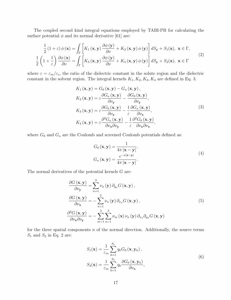
The coupled second kind integral equations employed by TABI-PB for calculating thesurface potential φ and its normal derivative [61] are:

1

2(1 + ε)φ (x) =

∫Γ

[K1 (x,y)

∂φ (y)

∂ν+K2 (x,y)φ (y)

]dSy + S1(x), x ∈ Γ,

1

2

(1 +

1

ε

)∂φ (x)

∂ν=

∫Γ

[K3 (x,y)

∂φ (y)

∂ν+K4 (x,y)φ (y)

]dSy + S2(x), x ∈ Γ

(2)

where ε = εm/εs, the ratio of the dielectric constant in the solute region and the dielectricconstant in the solvent region. The integral kernels K1, K2, K3, K4 are defined in Eq. 3.

K1 (x,y) = G0 (x,y)−Gκ (x,y) ,

K2 (x,y) = ε∂Gκ (x,y)

∂νy− ∂G0 (x,y)

∂νy,

K3 (x,y) = ε∂G0 (x,y)

∂νx− 1

ε

∂Gκ (x,y)

∂νx,

K4 (x,y) = ε∂2Gκ (x,y)

∂νx∂νy− 1

ε

∂2G0 (x,y)

∂νx∂νx,

(3)

where G0 and Gκ are the Coulomb and screened Coulomb potentials defined as:

G0 (x,y) =1

4π |x− y|,

Gκ (x,y) =e−κ|x−y|

4π |x− y|.

(4)

The normal derivatives of the potential kernels G are:

∂G (x,y)

∂νy=

3∑n=1

νn (y) ∂ynG (x,y) ,

∂G (x,y)

∂νx=−

3∑n=1

νn (y) ∂xnG (x,y) ,

∂2G (x,y)

∂νx∂νy=−

3∑m=1

3∑n=1

νm (x) νn (y) ∂xn∂ynG (x,y)

(5)

for the three spatial components n of the normal direction. Additionally, the source termsS1 and S2 in Eq. 2 are:

S1(x) =1

εm

Nc∑k=1

qkG0 (x,yk) ,

S2(x) =1

εm

Nc∑k=1

qk∂G0 (x,yk)

∂νx,

(6)

17

where Nc is the number of atoms in the solute molecule, and qk is the charge of the kthatom. Note that S1 is a linear superposition of the point charge electrostatic potentials, andS2 is a linear superposition of the normal derivatives of the potentials.

Given a surface triangularization with N elements – where xi and Ai are the centroidand area, respectively, of the ith triangle – the integral equations are discretized as:

1

2(1 + ε)φ (xi) =

N∑j=1j 6=i

[K1 (xi,xj)

∂φ (xj)

∂ν+K2 (xi,xj)φ (xj)

]Aj + S1(xi),

1

2

(1 +

1

ε

)∂φ (xi)

∂ν=

N∑j=1j 6=i

[K3 (xi,xj)

∂φ (xj)

∂ν+K4 (xi,xj)φ (xj)

]AJ + S2(xI).

(7)

The omission of the j = i term in the summation avoids the singularity of the kernels atthat point. Note that the right hand sides of these equations consist of sums of products ofkernels and the surface potential or its normal derivative. These are the analogues to theN -body potential in the treecode, with the surface potential or its normal derivatives playingthe role of the charges. In the discretized form, the total electrostatic energy of solvation isgiven by Eq. 8:

Esol =1

2

Nc∑k=1

qk

N∑j=1

[K1 (xk,xj)

∂φ (xj)

∂ν+K2 (xk,xj)φ (xj)

]Aj (8)

where qk is the charge on the kth atom of the solute molecule, and xk is its position.The matrix-vector products involve evaluation of the integral kernels over the surface

elements. These evaluations effectively take the form of an N -body potential: a sum over aset of N positions of products between a kernel and a “charge” at each position. In this case,the locations of the N particles are the centroids of the surface triangularization elements.A Cartesian particle-cluster treecode is used to compute matrix-vector products and reducethe computational cost of this dense system from O(N2) to O(N logN) for N points on thediscretized molecular surface [64]. In particular, to rapidly evaluate the N -body potentialat the N particle locations, the treecode subdivides the particles into a tree-like hierarchicalstructure of clusters. At each location, the potential contribution from nearby particlesis computed by direct sum, while for well-separated particle cluster interactions, a Taylorapproximation about the center of the cluster is used to evaluate the contribution. TheTaylor coefficients are calculated through recurrence relations. The resulting linear systemis then solved with GMRES iteration [103].

Because the integral equations are defined on the molecular boundary, the singularcharges are handled analytically and do not introduce the same issues present in grid-basedschemes. The integral equations also rigorously enforce the interface conditions on the sur-face, and the boundary condition at infinity is exactly satisfied. Thus, the boundary integralformulation can potentially be superior to other methods for investigating electrostatic po-tential on the boundary.

18

D.2 Boundary element calculation configuration

APBS users can invoke TABI-PB with the bem-manual flag in the ELEC section of the inputfile. Major options include:

• tree order 〈order〉: An integer indicating the order of the Taylor expansion for de-termining treecode coefficients. Higher values of 〈order〉 will result in a more accurate– but more expensive – calculations. A typical choice for this parameter is 3.

• tree n0 〈number〉: The maximum number of particles allowable in a leaf of thetreecode (clusters in the last level of the tree). A typical choice for this parameteris 500.

• mac 〈criterion〉: Multipole acceptance criterion specifies the distance ratio at whichthe Taylor expansion is used. In general, a higher value of 〈criterion〉 will result in amore accurate but more expensive computation; while a lower value causes more directsummations and forces the particle-cluster interaction to descend to a finer cluster level.A typical choice for this parameter is 0.8.

• mesh 〈flag〉: The software used to mesh the molecular surface; 0 = MSMS, 1 = Nano-Shaper’s SES implementation, and 2 = NanoShaper’s Skin implementation. See Fig-ure 2 for an example of surface meshes.

• outdata 〈flag〉: Type of output data file generated; 0 = APBS OpenDX format [104]and 1 = ParaView format [105].

Additional information about parameter settings is provided via the APBS website [19].TABI-PB produces output including the potential and normal derivative of potential forevery element and vertex of the triangularization, as well as the electrostatic solvation energy.Examples of electrostatic surface potential on the protein 1a63 are shown in Figure 2 by usingMSMS and NanoShaper.

E Analytical and semi-analytical method implementa-

tions

This appendix provides additional information about the analytical and semi-analytic meth-ods [29, 30] introduced in Section 3.4.

E.1 Analytical method (PB-AM) background

The solution to the PB-AM model is represented as a system of linear equations:

A = Γ · (∆ · T · A+ E), (9)

where A represents a vector of the effective multipole expansion of the charge distributions ofeach molecule, E is a vector of the fixed charge distribution of all molecules, Γ is a dielectricboundary-crossing operator, ∆ is a cavity polarization operator, and T is an operator that

19

transforms the multipole expansion from the global (lab) coordinates to a local coordinateframe. The unknown A determined using the Gauss-Seidel iterative method and can then beused to compute physical properties such as interaction energies, forces, and torques. Theinteraction energy for molecule i, (Ω(i)) is given in Eq. 10.

Ω(i) =1

εs

⟨N∑j 6=i

T · A(j), A(i)

⟩(10)

where εs is the dielectric constant of the solvent and 〈M,N〉 denotes the inner product.When energy is computed, forces follow as:

F(i) = ∇iΩ(i) =

1

εs[〈∇i T · A(i), A(i)〉+ 〈T · A(i),∇iA

(i)〉] (11)

By definition, the torque on a charge in the molecule is the cross product of its positionrelative to the center of mass of the molecule with the force it experiences. The total torqueon the molecule is a linear combination of the torque on all charges of the molecule, asillustrated in Eq. 12.

τ (i) =1

εs

[xH(i),yH(i),zH(i)

]×[∇iL

(i)]

(12)

where αH(i)n,m =

∑Mi

j=1 α(i)j γ

(i)n q

(i)j (ρ

(i)j )nYn,m(ϑ

(i)j , ϕ

(i)j ) , α = x, y, z, is a coefficient vector for

each of the charges in the molecule, Mi is the number of charges in molecule i, q(i)J is the

magnitude of the jth charge, and p(i)j =

[ρ

(i)j , ϑ

(i)j , ϕ

(i)j

]is its position in spherical coordinates.

For more details on the PB-AM derivation, see Lotan and Head-Gordon [29].

E.2 Semi-analytical method (PM-SAM) background

The derivation details of PB-SAM have been reported previously [31, 32], with the mainpoints being summarized in this section. The electrostatic potential (φr) of the system atany point r is governed by the linearized form of the PB equation:

−∇ · ε∇φ+ κ2φ = ρ, (13)

where κ is the inverse Debye length. Eq. 13 is a linearization of Eq. 1 for βqiφ 1. For thecase of spherical cavities, we can solve Eq. 13 by dividing the system into inner sphere andouter sphere regions, and enforcing a set of boundary conditions that stipulate the continuityof the electrostatic potential and the electrostatic field at the surface of each sphere. Theelectrostatic potential outside molecule (I) is described by:

φ(i)out(r) =

Nmol∑I=1

(4π

∫dΩ(I)

e−κ|r−r′|

|r − r′|h(I)(r′)dr′

)(14)

where h(r) is an effective surface charge that can be transformed into the unknown multipoleexpansion H(I,k) with inside molecule I and sphere k. In a similar manner, the interior

20

potential is given as

φ(i)in (r) =

N(I)C∑

α=1

1

|r − r(I)α |· q

(I)α

εin+

1

4π

∫dΩ(I)

1

|r − r′|f (I)(r′)dr′ (15)

where N(I)C is the number of charges in molecule I, qα is the magnitude of the α-th charge,

r(I)α =

[ρ

(I)α , θ

(I)α , φ

(I)α

]is its position in spherical coordinates, and f(r) is a reactive surface

charge that can be transformed into the unknown multipole expansion F (I,k). The reactivemultipole and the effective multipole, H(I,k), are given as:

F (I,k)n,m ≡

1

4π

∫dΩ(I,k)

f (I,k)(r′)

(a(I,k)

r′

)n+1

Y(I,k)n,m (θ′, φ′)dr′ (16)

H(I,k)n,m ≡

1

4π

∫dΩ(I,k)

h(I,k)(r′)

(r′

a(I,k)

)nin(κr′)Y

(I,k)n,m (θ′, φ′)dr′ (17)

where Yn,m is the spherical harmonics, Yn,m is the complete conjugate, and a(I,k) is the radiusof sphere k of molecule I. These multipole expansions can be iteratively solved using:

F (I,k)n,m = 〈I(I,k)

E,n,m,WF (I,k)〉 (18)

H(I,k)n,m = 〈I(I,k)

E,n,m,WH(I,k)〉 (19)

where WF (I,k) and WH(I,k) are scaled multipoles computed from fixed charges and polariza-tion charges from other spheres. I

(I,k)E,n,m is a matrix of the surface integrals over the exposed

surface:

I(I,k)E,n,m ≡

1

4π

∫φE

∫θE

Y(I,k)l,s (θ′, φ′)Y

(I,k)n,m (θ′, φ′) sin θ′dθ′dφ′ (20)

Using the above formalism, physical properties of the system, such as interaction energy,forces and torques can also be computed. The interaction energy of each molecule, (Ω(i)), isthe product of the molecule’s total charge distribution (from fixed and polarization charges)with the potential due to external sources. This is computed as the inner product between themolecule’s multipole expansion, (H(I,k)), and the multipole expansions of the other moleculesin the system, (LHN (I,k)) as follows:

Ω(i) =1

εs

N(I)k∑k

〈LHN (I,k), H(I,k)〉 (21)

which allows us to define the force which is computed as the gradient of the interactionenergy with respect to the position of the center of molecule I :

F (I) = −∇Ω(I) = − 1

εs

N(I)k∑k

fI,k = − 1

εs

N(I)k∑k

(〈∇LHN (I,k), H(I,k)〉+ 〈LHN (I,k),∇H(I,k)〉) (22)

As in the analytical PB-AM method, the torque on a charge in the molecule is the crossproduct of its position relative to the center of mass of the molecule with the force it expe-riences. For a charge at position P about the center of mass c(I) for molecule I, the torque

21

is given by the cross product of its position r(I,k)P with respect to the center of mass and

the force on that charge fP . We can re-express r(I,k)P as the sum of vectors from the center

of molecule I to the center of sphere k (c(I,k)) and from the center of sphere k to point P

(r(I,k)P ). The total torque on molecule I is then given by Eq. 23.

τ (I) =

N(I)k∑k

c(I,k) × fI,k +

N(I)k∑k

∑P∈k

r(I,k)P × fP (23)

where fI,k is given in Eq. 22 and

fP = − 1

εs

N(I)k∑k

(〈∇ILHN(I,k), H

(I,k)P 〉+ 〈LHN (I,k),∇IH

(I,k)P 〉) (24)

where

H(I,k)P,n,m = h(θp, φp)Y

(I,k)n,m (θp, φp) (25)

∇jH(I,k)P,α,n,m = [∇j h(θp, φp)]α Y

(I,k)n,m (θp, φp) (26)

where α = x, y, z. For the derivation of the PB-SAM solver please see the previous publica-tions [31, 32] .

E.3 PB-AM and PB-SAM configuration in APBS

PB-AM and PB-SAM have been fully integrated into APBS, and is invoked using the keywordpbam-auto or pbsam-auto in the ELEC section of an APBS input file. Major options include:

• runname 〈name〉: Desired name to be used for outputs of each run.

• pbc 〈length〉: Size of the periodic simulation/calculation domain.

• runtype dynamics: Perform a Brownian Dynamics simulation.

• ntraj 〈number〉: Number of Brownian Dynamics simulations to run.

• term 〈type〉 〈value〉 〈mol〉: Allows the user to indicate conditions for the terminationof each BD trajectory. The following values of 〈type〉 are allowed:

– time 〈time〉: A limit on the total simulation time.

– x or y or y or z or r and 〈>=〉 or 〈<=〉: Represents the approach of two moleculesto a certain distance r or certain region of space given by x or y or y. The operators>= and <= represent the corresponding inequalities.

The parameter 〈mol〉 is the molecular index that this condition applies. 〈mol〉 shouldbe 0 for time and for a termination condition of x, y or z, the molecule index that thistermination condition applies to.

22

• xyz 〈idx 〉 〈fpath〉: Molecule index 〈idx 〉 and file path 〈fpath〉 for the molecule startingconfigurations. A starting configuration is needed for each molecule and each trajec-tory. Therefore, jf there are m molecules and ntraj 〈n〉 trajectories, then the inputfile must contain m× n xyz entries.

• tolsp 〈val〉: Modify the coarseness of the molecular description. 〈val〉 is the distance(in A) beyond the solvent-excluded surface that the coarse-grained representation ex-tends. Increasing values of 〈val〉 leads to fewer coarse-grained spheres, faster calculationtimes, but less accurate solutions. Typical values for 〈val〉 are between 1 and 5 A.

The commands (keywords) not included in this list are used to specify system conditions,such as temperature and salt concentration. These parameters are similar to those foundin the ELEC section of a usual APBS run and are documented on the Contributions portionof the APBS website [19]. Additional information about parameter settings is provided viathe APBS website [19]. Examples of the electrostatic potentials produced from PB-AM andPB-SAM are shown in Figures 3 and 4, respectively.

References

[1] M. E. Davis and J A McCammon. “Electrostatics in biomolecular structure and dy-namics”. In: Chemical Reviews 90.3 (1990), pp. 509–521.

[2] M F Perutz. “Electrostatic effects in proteins”. In: Science 201.4362 (1978), pp. 1187–91.

[3] P Ren et al. “Biomolecular electrostatics and solvation: a computational perspec-tive”. In: Quarterly Reviews of Biophysics 45.4 (2012), pp. 427–91. doi: 10.1017/S003358351200011X.

[4] K A Sharp and B Honig. “Electrostatic interactions in macromolecules: theory andapplications”. In: Annual Review of Biophysics and Biophysical Chemistry 19 (1990),pp. 301–32. doi: 10.1146/annurev.bb.19.060190.001505.

[5] B Roux and T Simonson. “Implicit solvent models”. In: Biophysical Chemistry 78.1-2(1999), pp. 1–20.

[6] A Warshel et al. “Modeling electrostatic effects in proteins”. In: Biochimica et Bio-physica Acta 1764.11 (2006), pp. 1647–76. doi: 10.1016/j.bbapap.2006.08.007.

[7] M Fixman. “The Poisson-Boltzmann equation and its application to polyelectrolytes”.In: Journal of Chemical Physics 70 (1979), pp. 4995–5005.

[8] P Grochowski and J Trylska. “Continuum molecular electrostatics, salt effects, andcounterion binding–a review of the Poisson-Boltzmann theory and its modifications”.In: Biopolymers 89.2 (2008), pp. 93–113. doi: 10.1002/bip.20877.

[9] G Lamm et al. “The Poisson-Boltzmann Equation”. In: Reviews in ComputationalChemistry 19 (2003), pp. 147–365.

[10] B. Lee and F. M Richards. “The interpretation of protein structures: Estimation ofstatic accessibility”. In: Journal of Molecular Biology 55.3 (1971), pp. 379–400. doi:10.1016/0022-2836(71)90324-X.

23

[11] R. R. Netz and H. Orland. “Beyond Poisson-Boltzmann: Fluctuation effects and corre-lation functions”. In: European Physical Journal E: Soft Matter 1.2-3 (2000), pp. 203–214.

[12] B R Brooks et al. “CHARMM: the biomolecular simulation program”. In: Journal ofComputational Chemistry 30.10 (2009), pp. 1545–614. doi: 10.1002/jcc.21287.

[13] D A Case et al. “The AMBER biomolecular simulation programs”. In: Journal ofComputational Chemistry 26.16 (2005), pp. 1668–88. doi: 10.1002/jcc.20290.

[14] S Sarkar et al. “DelPhi web server: A comprehensive online suite for electrostaticcalculations of biological macromolecules and their complexes”. In: Communicationsin Computational Physics 13.1 (2013), pp. 269–284.

[15] AD Bochevarov et al. “Jaguar: A high-performance quantum chemistry software pro-gram with strengths in life and materials sciences”. In: International Journal of Quan-tum Chemistry 113.18 (2013), pp. 2110–2142.

[16] JA Grant, BT Pickup, and A Nicholls. “A smooth permittivity function for Poisson-Boltzmann solvation methods”. In: Journal of Computational Chemistry 22 (2001),pp. 608–640.

[17] Y. C. Zhou, M. Feig, and G. W. Wei. “Highly accurate biomolecular electrostaticsin continuum dielectric environments”. In: Journal of Computational Chemistry 29.1(2008), pp. 87–87. doi: 10.1002/jcc.20769.

[18] N A Baker et al. “Electrostatics of nanosystems: application to microtubules and theribosome”. In: Proceedings of the National academy of Sciences of the United Statesof America 98.18 (2001), pp. 10037–41. doi: 10.1073/pnas.181342398.

[19] “APBS website”. http : / / www . poissonboltzmann . org/. url: http : / / www .

poissonboltzmann.org/.

[20] Sriram Krishnan et al. “Design and evaluation of Opal2: A toolkit for scientific soft-ware as a service”. In: Services-I, 2009 World Conference on. IEEE. 2009, pp. 709–716. url: http://nbcr-222.ucsd.edu/opal2/dashboard.

[21] J C Phillips et al. “Scalable molecular dynamics with NAMD”. In: Journal of Com-putational Chemistry 26.16 (2005), pp. 1781–802. doi: 10.1002/jcc.20289.

[22] David Baker. “Rosetta website”. https://www.rosettacommons.org/. url: https://www.rosettacommons.org/.

[23] Jay Ponder. “TINKER website”. https : / / dasher . wustl . edu / tinker/. url:https://dasher.wustl.edu/tinker/.

[24] R Konecny, N A Baker, and J A McCammon. “iAPBS: a programming interface toAdaptive Poisson-Boltzmann Solver (APBS)”. In: Computational Science and Dis-covery 5.1 (2012). doi: 10.1088/1749-4699/5/1/015005.

[25] “iAPBS website”. https://mccammon.ucsd.edu/iapbs/. url: https://mccammon.ucsd.edu/iapbs/.

24

[26] M Holst, N Baker, and F Wang. “Adaptive multilevel finite element solution of thePoisson-Boltzmann equation I. Algorithms and examples”. In: Journal of Computa-tional Chemistry 21.15 (2000), pp. 1319–1342.

[27] N Baker, M Holst, and F Wang. “Adaptive multilevel finite element solution of thePoisson-Boltzmann equation II. Refinement at solvent-accessible surfaces in biomolec-ular systems”. In: Journal of Computational Chemistry 21.15 (2000), pp. 1343–1352.

[28] N A Baker et al. “The adaptive multilevel finite element solution of the Poisson-Boltzmann equation on massively parallel computers”. In: IBM Journal of Researchand Development 45.3-4 (2001), pp. 427–438.

[29] Itay Lotan and Teresa Head-Gordon. “An Analytical Electrostatic Model for SaltScreened Interactions between Multiple Proteins”. In: Journal of Chemical Theoryand Computation 2.3 (2006). PMID: 26626662, pp. 541–555. doi: 10.1021/ct050263p.eprint: http://dx.doi.org/10.1021/ct050263p.

[30] Lisa E. Felberg et al. “PB-AM: An open-source, fully analytical linear Poisson-Boltzmann solver”. In: Journal of Computational Chemistry 38.15 (2017), pp. 1275–1282. issn: 1096-987X. doi: 10.1002/jcc.24528.

[31] E-H Yap and T Head-Gordon. “New and Efficient Poisson-Boltzmann Solver for In-teraction of Multiple Proteins”. In: Journal of Chemical Theory and Computation 6.7(2010), pp. 2214–2224. doi: 10.1021/ct100145f.

[32] E. H. Yap and T. Head-Gordon. “Calculating the Bimolecular Rate of Protein-ProteinAssociation with Interacting Crowders”. In: Journal of Chemical Theory and Com-putation 9.5 (2013), pp. 2481–9. issn: 1549-9618 (Print) 1549-9618 (Linking). doi:10.1021/ct400048q. url: http://www.ncbi.nlm.nih.gov/pubmed/26583736.

[33] Donald Bashford. “An Object-Oriented Programming Suite for Electrostatic Effectsin Biological Molecules”. In: Scientific Computing in Object-Oriented Parallel En-vironments. Ed. by Yutaka Ishikawa et al. Vol. 1343. Lecture Notes in ComputerScience. Berlin: Springer, 1997, pp. 233–240.

[34] Garrett M. Morris et al. “AutoDock4 and AutoDockTools4: Automated docking withselective receptor flexibility”. In: Journal of Computational Chemistry 30 (2009),pp. 2785–2791. url: http://www3.interscience.wiley.com/cgi-bin/abstract/122365050/ABSTRACT.

[35] “Protein Data Bank Contents Guide: Atomic Coordinate Entry Format Description.Version 3.3”. http://www.wwpdb.org/documentation/file-format-content/format33/v3.3.html. 2012. url: http://www.wwpdb.org/documentation/file-format-content/format33/v3.3.html.

[36] “PDBx/mmCIF Dictionary Resources”. http://mmcif.wwpdb.org/. url: http://mmcif.wwpdb.org/.

[37] J. Westbrook et al. “PDBML: the representation of archival macromolecular struc-ture data in XML”. In: Bioinformatics 21.7 (2005), pp. 988–992. doi: 10.1093/

bioinformatics/bti082.

25

[38] Todd J Dolinsky et al. “PDB2PQR: an automated pipeline for the setup of Poisson–Boltzmann electrostatics calculations”. In: Nucleic Acids Research 32.suppl 2 (2004),W665–W667.

[39] T J Dolinsky et al. “PDB2PQR: expanding and upgrading automated preparationof biomolecular structures for molecular simulations”. In: Nucleic Acids Research 35(2007), W522–5. doi: 10.1093/nar/gkm276.

[40] “sed - a stream editor”. https://www.gnu.org/software/sed/manual/sed.html.url: https://www.gnu.org/software/sed/manual/sed.html.

[41] Chresten R. Sondergaard et al. “Improved Treatment of Ligands and Coupling Effectsin Empirical Calculation and Rationalization of pKa Values”. In: Journal of ChemicalTheory and Computation 7.7 (2011), pp. 2284–2295.

[42] H. Li, A. D. Robertson, and J. H. Jensen. “Very fast empirical prediction and ratio-nalization of protein pKa values”. In: Proteins 61 (2005), p. 704721.

[43] Emilie Purvine et al. “Energy Minimization of Discrete Protein Titration State Mod-els Using Graph Theory”. In: Journal of Physical Chemistry 120 (2016), pp. 8354–8360. doi: 10.1021/acs.jpcb.6b02059.

[44] J E Nielsen and G Vriend. “Optimizing the hydrogen-bond network in Poisson-Boltzmann equation-based pKa calculations”. In: Proteins 43.4 (2001), pp. 403–12.

[45] Junmei Wang, Piotr Cieplak, and Peter A. Kollman. “How well does a restrainedelectrostatic potential (RESP) model perform in calculating conformational energiesof organic and biological molecules?” In: Journal of Computational Chemistry 21.12(2000), pp. 1049–1074. doi: 10 . 1002 / 1096 - 987X(200009 ) 21 : 12<1049 :: AID -

JCC3>3.0.CO;2-F.

[46] A.D. MacKerell Jr., M. Feig, and C.L. Brooks III. “Extending the treatment of back-bone energetics in protein force fields: limitations of gas-phase quantum mechanicsin reproducing protein conformational distributions in molecular dynamics simula-tions”. In: Journal of Computational Chemistry 25.11 (2004), pp. 1400–1415. doi:10.1002/jcc.20065.

[47] Doree Sitkoff, Kim A. Sharp, and Barry Hong. “Accurate calculation of hydrationfree energies using macroscopic solvation models”. In: Journal of Physical Chemistry98.7 (1994), pp. 1978–1988.

[48] Paul Czodrowski et al. “Development, validation, and application of adapted PEOEcharges to estimate pKa values of functional groups in protein-ligand complexes”. In:Proteins 65.2 (2006), pp. 424–437. issn: 1097-0134. doi: 10.1002/prot.21110.

[49] J M J Swanson, S A Adcock, and J A McCammon. “Optimized Radii for Poisson-Boltzmann Calculations with the AMBER Force Field”. In: Journal of ChemicalTheory and Computation 1.3 (2005), pp. 484–93. doi: 10.1021/ct049834o.

[50] Chunhu Tan, Lijiang Yang, and Ray Luo. “How Well Does Poisson-Boltzmann Im-plicit Solvent Agree with Explicit Solvent? A Quantitative Analysis”. In: Journalof Physical Chemistry B 110.37 (2006), pp. 18680–18687. issn: 1520-6106. doi: 10.1021/jp063479b.

26

[51] Michael Holst. “Adaptive numerical treatment of elliptic systems on manifolds”. In:Journal of Computational Mathematics 15 (2001), pp. 139–191.

[52] “FEtk website”. http://www.fetk.org. url: http://www.fetk.org.

[53] Kaihsu Tai et al. “Finite element simulations of acetylcholine diffusion in neuromus-cular junctions”. In: Biophysical Journal 84.4 (2003), pp. 2234–2241. doi: 10.1016/S0006-3495(03)75029-2.

[54] Michael Holst and Faisal Saied. “Multigrid solution of the Poisson—Boltzmann equa-tion”. In: Journal of Computational Chemistry 14.1 (1993), pp. 105–113. doi: 10.1002/jcc.540140114.

[55] Z Chen, N A Baker, and G W Wei. “Differential geometry based solvation model I:Eulerian formulation”. In: Journal of Computational Physics 229.22 (2010), pp. 8231–8258. doi: 10.1016/j.jcp.2010.06.036.

[56] Z Chen, N A Baker, and G W Wei. “Differential geometry based solvation model II:Lagrangian formulation”. In: Journal of Mathematical Biology 63.6 (2011), pp. 1139–200. doi: 10.1007/s00285-011-0402-z.

[57] Z Chen et al. “Variational approach for nonpolar solvation analysis”. In: Journal ofChemical Physics 137.8 (2012), p. 084101. doi: 10.1063/1.4745084.

[58] M D Daily et al. “Origin of parameter degeneracy and molecular shape relationshipsin geometric-flow calculations of solvation free energies”. In: Journal of ChemicalPhysics 139.20 (2013), p. 204108. doi: 10.1063/1.4832900.

[59] D G Thomas et al. “ISA-TAB-Nano: a specification for sharing nanomaterial researchdata in spreadsheet-based format”. In: BMC Biotechnology 13 (2013), p. 2. doi:10.1186/1472-6750-13-2.

[60] Weihua Geng and Robert Krasny. “A treecode-accelerated boundary integral Poisson-Boltzmann solver for electrostatics of solvated biomolecules”. In: Journal of Compu-tational Physics 247 (2013), pp. 62–78.

[61] Andre Juffer et al. “The electric potential of a macromolecule in a solvent: A funda-mental approach”. In: Journal of Computational Physics 97.1 (1991), pp. 144–171.

[62] Michel Sanner, Arthur Olson, and Jean Claude Spehner. “Fast and robust compu-tation of molecular surfaces”. In: Proc 11th ACM Symp Comp Geom. ACM. 1995,pp. C6–C7.

[63] Sergio Decherchi and Walter Rocchia. “A general and robust ray-casting-based algo-rithm for triangulating surfaces at the nanoscale”. In: PLoS ONE 8.4 (2013), e59744.

[64] Peijun Li, Hans Johnston, and Robert Krasny. “A Cartesian treecode for screenedCoulomb interactions”. In: Journal of Computational Physics 228 (2009), pp. 3858–3868.

[65] D. Bashford and D. A. Case. “Generalized Born models of macromolecular solvationeffects”. In: Annual Review in Physical Chemistry 51 (2000), pp. 129–152. doi: 10.1146/annurev.physchem.51.1.129.

27

[66] W Humphrey, A Dalke, and K Schulten. “VMD: visual molecular dynamics”. In:Journal of Molecular Graphics 14.1 (1996), pp. 33–8, 27–8.

[67] Donald Ermak and J. A. McCammon. “Brownian dynamics with hydrodynamic in-teractions”. In: Journal of Chemical Physics 69.4 (1978), pp. 1352–1360.

[68] Schrodinger, LLC. “The PyMOL Molecular Graphics System, Version 1.8”. PyMOL.2015.

[69] “PyMOL website”. http://www.pymol.org. url: http://www.pymol.org.

[70] “VMD website”. http://www.ks.uiuc.edu/Research/vmd/.

[71] Graham T. Johnson et al. “ePMV Embeds Molecular Modeling into ProfessionalAnimation Software Environments”. In: Structure 19.3 (2011), pp. 293–303. doi: 10.1016/j.str.2010.12.023.

[72] “MGLTools (AutoDock, PMV, Vision) website”. http://mgltools.scripps.edu/.url: http://mgltools.scripps.edu/.

[73] “Chimera website”. https://www.cgl.ucsf.edu/chimera/. url: https://www.cgl.ucsf.edu/chimera/.

[74] E F Pettersen et al. “UCSF Chimera–a visualization system for exploratory researchand analysis”. In: Journal of Computational Chemistry 25.13 (2004), pp. 1605–12.doi: 10.1002/jcc.20084.

[75] “Jmol website”. http://jmol.sourceforge.net/. url: http://jmol.sourceforge.net/.

[76] Angel Herraez. “Biomolecules in the computer: Jmol to the rescue”. In: Biochemistryand Molecular Biology Education 34.4 (2006), pp. 255–261.

[77] D Koes. “3Dmol.js”. http://3dmol.csb.pitt.edu/. url: http://3dmol.csb.pitt.edu/ (visited on 2016).

[78] Nicholas Rego and David Koes. “3Dmol.js: molecular visualization with WebGL”. In:Bioinformatics 31.8 (2015), pp. 1322–1324. url: http://3dmol.csb.pitt.edu/.

[79] S Unni et al. “Web servers and services for electrostatics calculations with APBS andPDB2PQR”. In: Journal of Computational Chemistry 32.7 (2011), pp. 1488–91. doi:10.1002/jcc.21720.

[80] RO Dror et al. “Structural basis for modulation of a G-protein-coupled receptor byallosteric drugs”. In: Nature 503.7475 (2013), pp. 295–299.

[81] L Treuel et al. “Impact of Protein Modification on the Protein Corona on Nanopar-ticles and Nanoparticle-Cell Interactions”. In: ACS Nano 8.1 (2013), pp. 503–513.

[82] Silvia H. De Paoli et al. “The effect of protein corona composition on the interactionof carbon nanotubes with human blood platelets”. In: Biomaterials 35.24 (2014),pp. 6182–6194. issn: 0142-9612. url: http://www.sciencedirect.com/science/article/pii/S0142961214004657.

[83] J Lipfert et al. “Understanding nucleic acid-ion interactions”. In: Annual Review ofBiochemistry 83 (2014), pp. 813–41. doi: 10.1146/annurev- biochem- 060409-

092720.

28

[84] V A Roberts et al. “DOT2: Macromolecular docking with improved biophysical mod-els”. In: Journal of Computational Chemistry 34.20 (2013), pp. 1743–58. doi: 10.1002/jcc.23304.

[85] T. Evangelidis et al. “An integrated workflow for proteome-wide off-target identifica-tion and polypharmacology drug design”. In: International Conference on Bioinfor-matics and Biomedicine Workshops. IEEE. 2009, pp. 32–39. url: doi:%2010.1109/BIBMW.2012.6470348.

[86] E Spiga et al. “Electrostatic-Consistent Coarse-Grained Potentials for Molecular Sim-ulations of Proteins”. In: Journal of Chemical Theory and Computation 9.8 (2013),pp. 3515–3526. doi: 10.1021/ct400137q.

[87] Phillip J Stansfeld et al. “MemProtMD: Automated Insertion of Membrane ProteinStructures into Explicit Lipid Membranes”. In: Structure 23.7 (2015), pp. 1350–1361.

[88] S Richter et al. “webPIPSA: a web server for the comparison of protein interactionproperties”. In: Nucleic Acids Res 36.Web Server issue (2008), W276–80. doi: 10.1093/nar/gkn181.

[89] Gary A. Huber and J. Andrew McCammon. “Browndye: A software package for Brow-nian dynamics”. In: Computer Physics Communications 181.11 (2010), pp. 1896–1905. doi: 10.1016/j.cpc.2010.07.022.

[90] Michael Martinez et al. “SDA 7: A modular and parallel implementation of the sim-ulation of diffusional association software”. In: Journal of Computational Chemistry36.21 (2015), pp. 1631–45. doi: 10.1002/jcc.23971.

[91] Y Cheng et al. “Finite element analysis of the time-dependent Smoluchowski equa-tion for acetylcholinesterase reaction rate calculations”. In: Biophysical Journal 92.10(2007), pp. 3397–406. doi: 10.1529/biophysj.106.102533.

[92] Y Cheng et al. “Continuum simulations of acetylcholine diffusion with reaction-determined boundaries in neuromuscular junction models”. In: Biophysical Chemistry127.3 (2007), pp. 129–39. doi: 10.1016/j.bpc.2007.01.003.

[93] Y Song et al. “Continuum diffusion reaction rate calculations of wild-type and mutantmouse acetylcholinesterase: adaptive finite element analysis”. In: Biophysical Journal87.3 (2004), pp. 1558–1566.

[94] A H Elcock. “Molecular simulations of diffusion and association in multimacromolec-ular systems”. In: Methods in Enzymology 383 (2004), pp. 166–98. doi: 10.1016/S0076-6879(04)83008-8.

[95] P Mereghetti and RC Wade. “Atomic Detail Brownian Dynamics Simulations of Con-centrated Protein Solutions with a Mean Field Treatment of Hydrodynamic Interac-tions”. In: Journal of Physical Chemistry 116.29 (2012), pp. 8523–8533.

[96] Michael J Holst. “Clean Object-Oriented C”. http://fetk.org/codes/maloc/api/html/index.html.

[97] Michael K. Gilson, Kim A. Sharp, and Barry H. Honig. “Calculating the electro-static potential of molecules in solution: Method and error assessment”. In: Journalof Computational Chemistry 9.4 (1988), pp. 327–335. doi: 10.1002/jcc.540090407.

29

[98] W. Im, D. Beglov, and B. Roux. “Continuum Solvation Model: Computation of elec-trostatic forces from numerical solutions to the Poisson-Boltzmann equation”. In:Computer Physics Communications 111 (1998), pp. 59–75.

[99] M. J. Schnieders et al. “Polarizable atomic multipole solutes in a Poisson-Boltzmanncontinuum”. In: Journal of Chemical Physics 126 (2007), p. 124114. url: https://www.ncbi.nlm.nih.gov/pubmed/17411115.

[100] Robert E. Bruccoleri et al. “Finite difference Poisson-Boltzmann electrostatic cal-culations: Increased accuracy achieved by harmonic dielectric smoothing and chargeantialiasing”. In: Journal of Computational Chemistry 18.2 (1997), pp. 268–276.

[101] Mafalda Nina, Wonpil Im, and Benoit Roux. “Optimized atomic radii for proteincontinuum electrostatics solvation forces”. In: Biophysical Chemistry 78.1-2 (1999),pp. 89–96. doi: 10.1016/S0301-4622(98)00236-1.

[102] D G Thomas et al. “Parameterization of a geometric flow implicit solvation model”.In: Journal of Computational Chemistry 34.8 (2013), pp. 687–95. doi: 10.1002/jcc.23181.

[103] Y. Saad and M. Schultz. “GMRES: A generalized minimal residual algorithm for solv-ing nonsymmetric linear systems”. In: Journal of Scientific and Statistical Computing7 (1986), pp. 856–869.

[104] “OpenDX”. http://fetk.org/codes/maloc/api/html/index.html. url: http://www.opendx.org/.

[105] James Ahrens, Berk Geveci, and Charles Law. ParaView: An End-User Tool for LargeData Visualization. Elsevier, 2005.

30