NASA-CR-ZOI051

- fJ

Research Institute for Advanced Computer ScienceNASA Ames Research Center

A fast Poisson solver for unsteady

incompressible Navier-Stokes Equations

on the half-staggered grid

G. H. Golub, L. C. Huang, H. Simon and W.-P. Tang

RIACS Technical Report 95.07 April 1995

https://ntrs.nasa.gov/search.jsp?R=19960026757 2018-08-30T11:28:36+00:00Z

A fast Poisson solver for unsteady incompressible

Navier-Stokes Equations on the half-staggered grid

G. H. Golub, L. C. Huang, H. Simon and W.-P. Tang

The Research Institute for Advanced Computer Science is operated by Universities Space Research

Association, The American City Building, Suite 212, Columbia, MD 21044 (410)730-2656

Work reported herein was supported in part by NASA under contract NAS 2-13721 between

NASA and the Universities Space Research Association (USRA).

A fast Poisson solver for

Navier-Stokes Equations

unsteady incompressible

on the half-staggered grid

Abstract. In this paper, a fast Poisson solver for unsteady, incompressible Navier-Stokes equations

with finite difference methods on the non-uniform, half-staggered grid is presented. To achieve this, new

algorithms for diagonalizing a semi-definite pair are developed. Our fast solver can also be extended

to the three dimensional case. The motivation and related issues in using this second kind of staggered

grid are also discussed. Numerical testing has indicated the effectiveness of this algorithm.

Key words, fast solver, generalized eigenvalues, incompressible Navier-Stokes equations.

AMS(MOS) subject classifications. 15A22, 35Q30, 65F15, 65M06, 76D05

o

(INSE)

(1)

(2)

Introduction. Consider the unsteady incompressible Navier-Stokes equations

_ + u + v + grad p = a div grad w

div w = 0

where w = (u, v)', in a two-dimensional region _ with initial condition

w(x,y,0) = w°(x,y) in fl

satisfying the constraint condition (2), and boundary condition

w(x,y,t) = wb(x,y,t) on 0_2.

The boundary condition on Ogt satisfies the consistency condition

(3) ¢ w.ds = 0.JO fl

The main difficulty in the solution of this problem is that the unsteady INSE is not

entirely evolutionary; it is subject to the divergence-free constraint (2). The projection

method, proposed by Chorin [3] and Temam [20], proved to be very effective and its

variants are widely used in many applications. With this method, some auxiliary ve-

locity is found and then projected into the divergence-free space via the solution of a

Poisson equation for some form of the pressure. For example, let the discretization of

(1) and (2), after linearization of nonlinear terms, be

£w(4) 'A----t-+ m/kw + V¢ = E

(5) V.w=0

where _w = w TM - w '_, A represents the discretization of convection and diffusion,

V and V. the discretization of grad and div respectively, ¢ = p,,+l _ p,_ the pressure

increment, and E includes all known terms at the nth level. With an approximate

factorization, Eq. (4) is put into the following fractional steps

(6) ,_w + AAxw = EAt

where Aw = _ - w" (_ is called the auxiliary velocity) and

W n+l -- _r

(7) At + V¢ = 0.

Now, applying the discrete divergence to (7), we obtain the discrete Poisson equation

for ¢:

V._

(s) v2¢- At

in which the discrete divergence free condition (5), V. w "+1 = 0 has been enforced.

The solution process is then:

U U U

V

V

V

P

U

P

U

P

V • V •P P

U U

V • V •P p

U U

V • V •P P

V

V

V

U U --U--

ofv u,vpe pe I P*

U_,V-- U_V-- U_V-- U_V

Il+.I+.I1+.U_V-- U_,V-- U,_V-- U._V

U.jV-- U_,V-- U.j.V-- U,_V

Fro. 2. Half-Staggered Grid

• Find _r by (6).

* Solve the discrete Poisson equation (8) for $.

• Update w TM by (7).

For a more detailed account with the boundary condition treatment, see [10].

The constraint (5) causes difficulties in the choice of the mesh, the coordinate

system and the related discrete Poisson equation, etc., of the solution method. For a

rectangular region f_, the usual staggered mesh (u, v and p staggered mesh as shown

in Fig. 1) is most frequently used. With this mesh, no pressure boundary condition is

needed, which is mathematically correct. Let the discretized linear system of equations

of (8) be denoted as

(9) L<:I)= R,

where • is the unknown vector of size, say, M. With this mesh, L is of rank M -

1; the constraint on the right hand side R reduces to an approximation of (3), and

the solution _ is unique up to a constant. For a rectangular region with uniform

or nonuniform mesh intervals, direct solvers from the FISHPACK have proved to be

most efficient, see [2, 16] for example. Also for the usual staggered mesh, the finite

difference approximation of (1) is the same as the finite volume approximation. In

addition, 27p and V. w are straightforward without any interpolation. However, u and

v involve different finite volumes and near the boundary half interval differencing is

necessary, which are inconveniences. More serious is the problem on curvilinear meshes

in arbitrary regions; there the extension of the usual staggered mesh will lose many

of the above advantages, see [17] for instance. Hence, the half-staggered mesh (w, p

staggered as shown in Fig. 2 was studied in [10, 11]. This mesh was first proposed

in [5] for the unsteady INSE; it was recently used in [1] with a different discretization

of projection, for example; but it is not used in practical computation in general. For

steady-state INSE, this mesh was used and investigated for FEM in [15] and for the

Galerkin formulation in [18].

The advantages of this mesh for the unsteady INSE are: no pressure boundary

condition is required; the finite difference approximation of (1) is the same as the finite

volume method with the same finite volume for u and v; Vp and _7.w involve only simple

averages, and there is no half interval differencing near the boundary. Most important

is the extension of this staggering to curvilinear meshes in arbitrary regions. As the

velocity components are at the same point, it is easily transformed to, say, contravariant

components for finite volume formation, for approximation of div w, and for boundary

conditions, etc.. The disadvantage of this mesh is the nature of the discrete Poisson

equation (8), where L is of rank M - 2. There is an additional constraint and the

solution qb may have oscillations; see the next section.

As the first step to this problem, we consider rectangular regions with nonuniform

meshes. Since (9) is to be solved at every time step for the unsteady INSE, efficient

solvers are necessary and this is the subject of this paper.

2. Diseretization. Consider a rectangular region with a nonuniform mesh, schemat-

ically show in Fig. 3. We generate the nonuniform mesh by some smooth transformation

x((), y(r/), with a uniform mesh in the computational (r/region, and approximate

- by -Ox dx O( _x 5x A(

where (_ on the right hand side denotes centered differencing, and similarly for O/Oy.

Then for every interior w point

(10)

j+ 1 1

[ ¢_+1,k+1 - ¢_,k+1 ¢_+1,k -- ¢_,k ]1 Xj+ 1 Xj + Xj+ 1 Xj

= 2 Cj+l,k+l Cj+l,k Cjrk+l Cj,k

Yk+l Yk + Yk+l xk

and (7) on all the interior w point can be written as

W n+l - W

(11) At + GO = 0

where G is the gradient matrix for the solution vector (P. For every interior ¢ point, or

rather every (j, k) cell,

1 1 [(uj+_,k+ _ + u. _ _ ( 3-_,k+_ + uj-½,k-½ ]V'Wij'k : 2Zj..{_l--Xj_½ 1 1 3-l--_,k-_)-- U" , 1 )

dxl dx2 dx3 dx4 _,j gi,j hio

dy3

dy2

dyl

di,)i,j

ai,j bi,j ci,j

ei,j

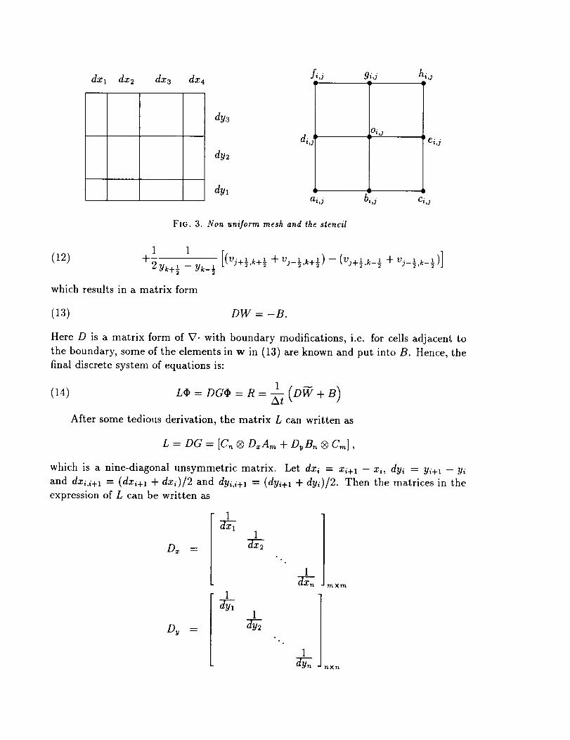
FIG. 3. Non uniform mesh and the stencil

(12) -_ 1 1 [(vj+½,k+ _ + vj__,k+_)_, -- (v._+_,k__ _ + v.j__,k__)]_2 Yk+½ - Yk-½

which results in a matrix form

(13) DW = -B.

Here D is a matrix form of V. with boundary modifications, i.e. for cells adjacent to

the boundary, some of the elements in w in (13) are known and put into B. Hence, the

final discrete system of equations is:

+(14) L(I) = DG¢ = R = -_

After some tedious derivation, the matrix L can written as

L = DG = [Ca ® D,A,.,, + D_B,_ ® Cm],

which is a nine-diagonal unsymmetric matrix. Let dxi = xi+l - xi, dyi = yi+l - yi

and dxi,i+l = (dxi+l + dxi)/2 and dyi,i+l = (dyi+l + dyi)/2. Then the matrices in the

expression of L can be written as

Dx

Dy

1

1

1

1

1

1

m Xrn

nXn

1 1

1 2

• .

• °

2

1

1

A,r¢l,

-(,_+_.°

'" " ") 1"" 1 +_= 1 - 1

• 1 ") 1""B. = I ___+ I .

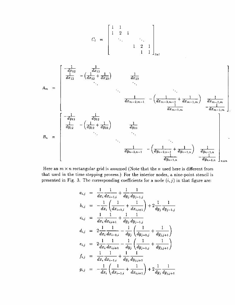
Here an m × n rectangular grid is assumed (Note that the n used here is different [rom

that used in the time stepping process.) For the interior nodes, a nine-point stencil is

presented in Fig. 3. The corresponding coefficients for a node (/,J) in that figure _re:

1 ! 1 1

bi,j ----- dxi \axi-l,i

I I I 1

dyj dy_-_,J

I ( I_./____+1 I _ _ _I |. . d?cj,j+_}

1 1

fi,j = dxi dxi-l,i dyj dyj,j+l 1

_ + 2_ ay.+,1 li_+

@i,j _" -- dx-"_ dxi-l,i dzi,i+t

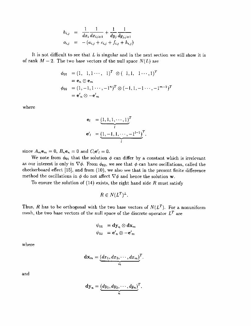
1 1 1 1hi,j - +

dxi dxi,i+l dyy dyy,y+l

oi,y = -- (ai,j + ci,j + fi,i + hi,i)

It is not difficult to see that L is singular and in the next section we will show it is

of rank M - 2. The two base vectors of the null space N(L) are

¢ol =(1, 1,1..., 1) T Q( 1,1, 1...,1) T

= en @ em

¢02 =(1,-1,1"",-1") T®(-1,1,-1...,-lm-a) r

= etn ® --etm

where

el =(1,1,1,...,1) r

I

e'l = (1,-1, 1,...,-1_-1) T.• y •

l

since Amem = 0, Bnen = 0 and Cle't = 0.

We note from ¢01 that the solution ¢ can differ by a constant which is irrelevant

as our interest is only in V¢. From ¢o2, we see that ¢ can have oscillations, called the

checkerboard effect [15], and from (10), we also see that in the present finite difference

method the oscillations in ¢ do not affect V¢ and hence the solution w.

To ensure the solution of (14) exists, the right hand side R must satisfy

R C N(LT) L.

Thus, R has to be orthogonal with the two base vectors of N(LT). For a nonuniform

mesh, the two base vectors of the null space of the discrete operator L T are

_ox = dy,_ ®dxm

_'o2 = etn Q--elm

where

dx_ = (dxl,dz2,...,dxm) T.

m

and

dyn = (dya , dy2, . . . , dy,Q T.

n

This can be verified by multiplying directly with the matrix L T.

LT_ol -:- [Cn Q AmDx + B,_Dy ® Cm] dy, ® dxm

= C_dy n ® AmDxdxm + B,_Dydy n ® Cmdxm

= 0

LTIP02 : [Cn ® A_Dx + B,_Dy ® C_] e',_ ® -e'm

= -C,_e',_ ® AmDxe'm - B,_Dye',_ ® Cme'm

= 0

since AmD_dxm = O, BnDudy,_ = 0 and Cte'l = O.

In [15], Sani investigated the solution of (13) and gave the base vectors of N(D T)

to be _01 and _02. He showed that the constraint ¢oTIB = 0 reduces to a discrete form

of (3), and ¢0T2B = 0 yields a constraint for the tangential velocity component on the

boundary•

For the unsteady INSE, the interest is in the solution of (14). Due to the divergence

form of R, _,_DW will cancel out, leaving CTR = (_TaB)/At. Hence, the constraint

¢TR = 0 is a discrete form of (3). ¢TR = 0 will also hold if (5) holds for some velocity

field with the given boundary condition, i.e. (13) holds for some W, for example, the

initial velocity field with time independent boundary condition•

When dxi _/kx and dyi =--Axy are constant, the matrix L is symmetric and has a

simpler form

where

AI=1

1 -2 1

1 -1lxl

In particular, when Axi = Ayi = h, the discretization is a well known skewed five point

stencil (see Fig. 4).

3. Fast solver. As we mentioned in the introduction, since the matrix equation

(9) must be solved every time step, an efficient solver is essential. Fast solvers for

the sum of two matrix tensor products were discussed in the first author's paper[2].

Later, L. Kaufman and D. Warner [13] provided a generalization to the higher order

discretization case. In particular, the eigen-decomposition applused in [2] is replaced

by a generalized eigenvalue and eigenvector problem. If we examine the formula of the

matrix L, it is clear that generalized eigen-decomposition is needed to develop our fastsolver• For a matrix of the form

AQB+CQE,

2 2

• 0 •

• o •

2 2

FIG. 4. Skewed five point stencil

the key step in developing a fast algorithm in [2, 13] was to simultaneously diagonalize

the matrices B and E by a matrix Z for which

ZTBZ = I, ZTEZ = D,

where B and E are symmetric and positive definite. There are two obvious problems

which cause these algorithms not to be directly applicable here. The first problem is

that the matrices L, D=Am and DuBn are not symmetric. The second problem is the

singularity of the matrices Am, Ct and B,_. Many of the effective generalized eigenvalue

algorithms [4, 8, 12, 21] for diagonalizing two banded matrices simultaneously need

the matrix pair to be nonsingular and symmetric. Unfortunately, both Am and Ct are

singular and D=Am is unsymmetric and thus a new approach is needed.

3.1. Equal-spaced in one direction. Assume the mesh is equal-spaced in one

direction, say the x direction.

Let Axi = Ax, i = 1,...,m. Then the matrix L can be written as

(15) L = [_-_C,_ ® A'_ + DyBn ® C_] .

Though the matrix L is not symmetric, both -A_ and C_ are symmetric, semi-definite

matrices. We can show the following result.

THEOREM 3.1. There exists a matrix Z such that

zTc2z = -A'_

zT s2z = Cm

where the diagonal elements ci, si of C and S satisfy

ci2 + s i2= 1, O _< ci,si _< 1 i= 1,... m.

Proof. The proof is a natural generalization of the result presented in [21], where a

pair of symmetric and definite matrices is considered.

There exist two orthogonal matrices T1 and T2 such that

-A" = T,D_T T,

Cm = T_DIT T,

where Di, i = 1,2 are diagonal matrices with non-negative diagonal elements. Now,construct

W= D2TT =QR

where Q, R make up the QR decomposition of the matrix W. Then partition matrix

Q as follows:

(16) Q= Q2

Applying Stewart's theorem[19], we have from the Singular Value Decomposition(SVD)[7]

Q1 = UlCV

Q2 = U2SV2

where /]1, U2, 1/1 and ½ are all orthogonal matrices and C, S are diagonal matrices

diag(c,) and diag(si), respectively. Then from (16) and the orthogonality of Q,

¼ =½=V

and

Therefore, we have

-A"

where

2 1c_ + S i = .

= T1D_T T = RTvTc2vR = zTc2z,

Cm = 2 TT2D2T _ = RTvTs2vR = zT s2z,

Z= VR.

0

After the simultaneous diagonalization of the matrices Am and Cm is achieved,

the fast solver in this case is similar to the Buzbee-Golub-Nilson or Kaufman-Warner

algorithm. First, the matrix equation (15) can be transformed into a tridiagonal matrix

equation as follows:

(I ® Z -r) L (I ® Z -1) = INZ-T[ 1C ],,@A" +DuB,_®Cm IQZ -1

_ -T i -11 C,_ ® Z AmZ + D_B,_ ® z-TCm Z-iAx 2

-1

- Ax2C,, ®C 2 + D_Bn ®S _

= i It,

where L" is a tridiagonal matrix. A simple permutation matrix transforms L" into a

block diagonal matrix. The diagonal elements are n x n tridiagonal matrices. The

solution of these tridiagonM matrices is trivial. In particular, they can be implemented

on a vector or parallel computer efficiently.

For a regular mesh, Ax = Ay = h, this block diagonal matrix has a very simple

form. We show the following result.

TttEOREM 3.2. The rank of the matrix L for regular mesh is of ran - 2.

Proof. We know that both A'_ and Cm have only one zero eigenvalue and N(A_) fl

N(Cm) = 0. Therefore, the two zero diagonal elements cq. and sj. in C and S will not

be in the same location. It is easy to arrange them such that cl = 0 and sm = 0. After

permuting the matrix L" to a block diagonal matrix, the first and last diagonal block

matrix will be:

T1 8 2 A' Tn 2: _ erich,l'an,

respectively. Each has only one zero eigenvalue. The rest of the diagonal block matrices

are of the form

(17) Ti 2 2 t= -c iC,_ + s iA,_, i = 2,...n - 1,

where c_ + s_ = 1. When c; = s_, (17) reduces to a diagonal matrix

diag{1,2,...,2, 1},

and it is not singular. If ci 7L si, Ti is a tridiagonal matrix, viz

T, = (-4 + g)

--a 1

1 -2a

".,

I 1where I 1- = 28 i -- C i

1

°,°

1 -2a 1

1 -a

> 1, and hence Ti is non-singular. El

lxl

We conjecture that this is true in general. Numerical computations support our

conjecture.

As we discussed in the previous section, the solutions of the matrix equation (14)

can differ by a linear combination of the two base vectors in N(L). Some special

attention needs to be paid to the solution of linear systems involving the first and last

tridiagonal submatrices 7'1 and Tin.

3.2. General case. For a general non-uniform grid, the simultaneous diagonal-

ization of both matrix D_Am and Cm by a single matrix can not be achieved. However,

the generalized eigenvectors 1 can still be used to achieve the same purpose with two

1 It is not difficult to see that the generalized eigenvalue problem:

D_A,,,,z = ACmx

different matrices. Recall the matrix equation:

(19)

where

L¢= R

_iD_Amvi = cqCmvi.

Let 73_ and :De be two diagonal matrices whose diagonal elements are ai and _i, respec-

tively. We have

D_A_ V_D_ = C_ V_D_

where matrix V = [vl,vl,'",vm]. Since we know that each matrix Am and Cm has one

zero eigenvalue, it is clear that each of :Da and Dc has one zero diagonal element. Due

to the orthogonality of the null spaces of N(Am) and N(Cm), the two zero diagonal

elements will not be in the same location. We arrange the generalized eigenvectors suchthat

Then we construct a matrix

a_ = 0; fix = 0.

(21) U = [DxAm[vl, v2,....Vm--l], Cmvm].

It is not difficult to see that

U-_(DxAm)V =

and

U-'CV =

0

1

1

°.°

1

0

is a discrete approximation of the eigenvalue problem

(18) - y" = Ay, y'(0) = y'(1) = 0

on a non-uniform grid. Therefore, this pencil is diagonalizable. Our extensive numerical testings withrandomly non-uniform grid have verified this observation. The eigenvectors are approximations of the

eigenfunctions of (18).

(20) L = DG = [C,_ ® D_Am + DvB,_ ® Cm].

The QZ algorithm [7, 14] is used to compute the generalized eigenvalues (ai,13i) and

its corresponding eigenvectors vi such that

Thus, the tridiagonalization of (20) can be achieved as follows:

(I,_ ® U-1)L(In ® V) = (L, ® U -1 ) [On @ D_A_ + D_,B,_ ® C_] (I,_ ® V)

= C,_ ® U-1D_AmV + DuBn ® U-1CV

= C,_@'[m+DyB,_®_Dx

= L.

Here, the matrix L has three non-zero diagonals with a bandwidth of m. The resulting

matrix equation will be

where

(In (_ U-')L(In @V)(ln @V-') ¢_ = (In @U-1)R

L_ = h,

= (I,_®V-')#h = (i_®u-a)n.

We start with an ordering of the grid nodes first in the x direction, then in the y

direction. Let P be the permutation matrix, which reorders the grid nodes first in the

y direction, then in the x direction. We have

(PL,P)(P_) = PR£_ = k,

where £ = PZ, P, _ = P_ and /_ = PR. The matrix £ is a block diagonal matrix in

which each diagonal element T,- is an n x n tridiagonal matrix:

and

T1 = Cn

T, = Cn+ _3iD BnY

Oli

Tm = DyBn

(i = 2,3,---,m - 1)

The solutions of the T[s are trivial, but, some attention should be paid to the first

one and last one, since both T1 and T,,, are rank n - 1 and the top left (n - 1) x

(n - 1) submatrices of T1 and Tm are not singular. We can solve the two non-singular

submatrices and assume the last element of the solution is zero. Using this approach,

the contribution of the two null space base vectors of L is set to be zero and this will

not affect the final solution of the INSE. The final solution of (19) is

_=(I,_®V)P_.

The fast solver can be

1. Preprocess.

(a) Compute the

(DxAm,Cm).

(b) Compute the

(c) Form the LU

Note that this step

INSE. The cost of

of step (a) and (b)

2. Solve

summarized as follows:

generalized eigen-decomposition (79a,79c, V) of the pencil

LU decomposition of the matrix U given in (21).

decompositions of the matrices Ti.

is needed once at the beginning of the solution process of the

it can be amortized over many time steps. The complexity

is O(ma), and of (c)is O(nm).

(I ® U)/_ = R.

The complexity is O(nm2).3. Solve

/,_ =/_ = P/_.

The complexity of this step is O(nm).

4. Compute

¢=(INV)P_

The complexity of this step is O(nm2).

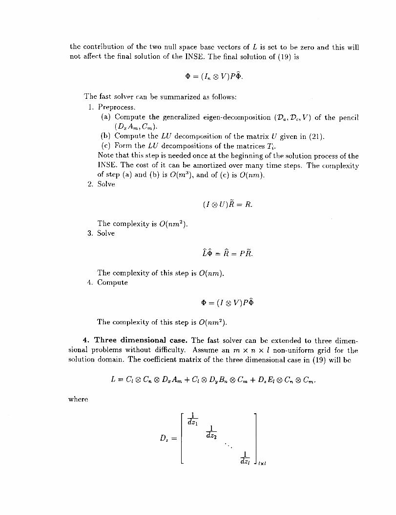
4. Three dimensional case. The fast solver can be extended to three dimen-

sional problems without difficulty• Assume an m x n x l non-uniform grid for the

solution domain. The coefficient matrix of the three dimensional case in (19) will be

L = Ct @ C,, ® D_:Am + Ct ® Du B,_ ® C,,, + D, Et ® C,, ® C_.

where

1

Dz

1

1

lxl

and

El =

1 1

1

1dzl-2,l-1 (1+1) 1dzl- ,l-1

1 1 l-i,l lxl

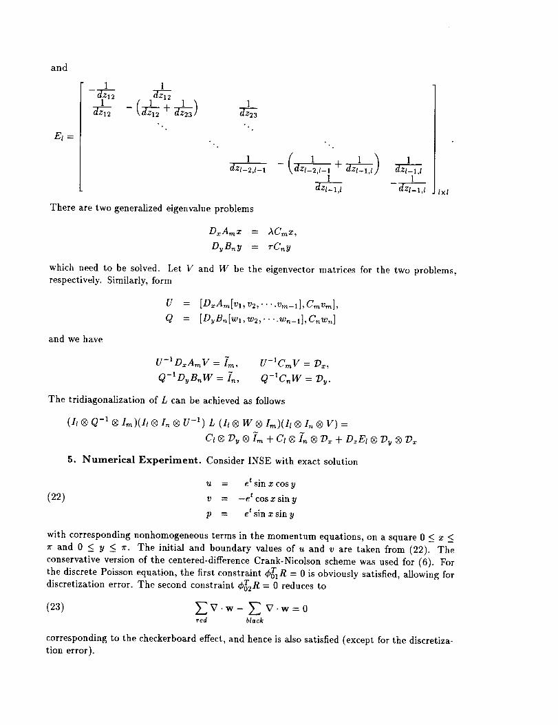
There are two generalized eigenvalue problems

DxAmx = ACmx,

DvB,_y = rC,_y

which need to be solved. Let V and W be the eigenvector matrices for the two problems,

respectively. Similarly, form

U = [D:_Am[vl,v2,'".vm-1],Cmv,,_],

Q = [DyB,_[w,,w2,....wn_,],Cnwn]

and we have

The tridiagonalization of L can be achieved as follows

(h ® Q-_ ® Im)(Ii @ I,_ ® U -_) L (Ii ® W ® Im)(I1 ® In ® V) =

Cl ® l_y ® "ira+ Cl ® I',_ ® l_:: + Dz El ® _y ® D_

5. Numerical Experiment. Consider INSE with exact solution

(22)

u = e tsinxcosy

v = --e t cosx siny

p = e tsinxsiny

with corresponding nonhomogeneous terms in the momentum equations, on a square 0 < x _<

r and 0 < y < r. The initial and boundary values of u and v are taken from (22). The

conservative version of the centered-difference Crank-Nicolson scheme was used for (6). For

the discrete Poisson equation, the first constraint ¢0T1R = 0 is obviously satisfied, allowing for

discretization error. The second constraint ¢0T2R = 0 reduces to

(23) Zv.w- Z v.w=ored black

corresponding to the checkerboard effect, and hence is also satisfied (except for the discretiza-

tion error).

On a 64 × 64 nonuniform mesh with mini(dxi) = mini(dyi) ,_ 3.3 × 10 -2 and maxi(dxi) =

maxi(dyi) _ 7.6 × 10 -2, the fast solver developed herein took 0.13 sec CPU time on the

100MHz Indigo R4000 workstation for each solution of (14), with residual _ 0.4 • 10 -3 and

maxij(V • w) _ 0.1 • 10 -3. There was no apparent oscillation in pressure, but adding ±1,

say, to the initial pressure at alternate cells (the red and black cells) will cause an oscillating

pressure distribution as shown in Fig 6 for t = 1. As we indicated earlier, the oscillation in p

has no effect on the solution of u and v shown in Fig. 5, nor any effect on the solution process.

In contrast, solving the same problem using an adaptive multigrid method [10] took six

times more CPU time. This version of the multigrid is not very effective in this application,

presumably due mainly to the treatment for the second constraint.

U V

3.

2,

1,

O,

-1,

-2.

-3:SO

6O

4O

20

0 0

6O

40

2O

3160 50 40 30 20 10" 0_0 20

FIG. 5. Solution u and v at t = 1

6. Conclusion. We have developed a fast Poisson solver for the unsteady incompressible

Navier-Stokes Equation with finite difference methods on the non-uniform, half-staggered

grid. Due to the efficiency of this method, it is possible to solve the unsteady flow with

Re = 10,000 [9]. Although this method can only be applied to an orthogonaJ rectangular

grid, it can be used as a preconditioner or in a domain decomposition scheme for general

applications. Our next project will be development of effective solvers for unsteady INSE on

an irregular domain with curvilinear grid.

[1] J.

[2] B

[31A.

[4] C.

[5] M.

REFERENCES

B. BELL, P. COLELLA, AND H. M. GLAZ, A second-order projection method for the incom-

pressible Navier-Stokes equations, Journal of Computational Physics, 85 (1989), pp. 257-283.

BUZBEE, G. GOLUB, AND C. NILSON, On direct methods for solving Poisson's equation, SIAM

Journal on Numerical Analysis, 7 (1970), pp. 627-656.

J. CHORIN, Numerical solution of Navier-Stokes equations, Mathematics of Computation, 22

(1968), pp. 745-762.

R. CRAWFORD, Reduction of aa band-symmetric generalized eigenvalue problem, Comm.

ACM., 16 (1973), pp. 41-44.

FORTIN, R. PEYRET, AND R. TEMAM, Calcul des ecoulements d'un fluide visqueux incom-

pressible, J. Mec, 10 (1971), pp. 357-390.

Oscillating P

-170 6o

5o 204o 302o

1o o o

FIG. 6. Oscillating pressure at t = 1

60

40

[6] G. GOLUB AND C. V. LOAN, Matrix Computations, second edition, The Johns Hopkins UniversityPress, Baltimore, MD, 1989.

[7] G. GOLUB AND V. E. LANGLOIS, Direct solution of the equation for the Stokes stream function,

Computer Methods in Applied Mechanics and Engineering, 19 (1979), pp. 391-399.

[8] R. G. GRIMES, J. G. LEWIS, AND H. D. SIMON, A shifted block Lanczos algorithm for solving

sparse symmetric generalized eigenproblems, SIAM Journal on Matrix Analysis and Applica-tions, 15 (1994), pp. 228-272.

[9] L. C. HUANG, J. OLIGER, W.-P. TANG AND Y. D. WU, Toward efficient and robust finite

difference schemes for unsteady incompressible Namer-Stokes equation on the half staggeredmesh, Sixth International Symposium on CFD, (1995).

[10] L. C. HUANG, On boundary treatment for the numerical solution of the incompressible Navier-

Stokes equations with finite difference methods, J. Comput. Math, (1994).

[11] --, On the staggered mesh 11for the finite difference solution of the unsteady incompressible

Namer-Stokes equations, J. Comput. Math, (1994). Submitted.

[12] L. KAUFMAN, An algorithm for the banded symmetric generalized matriz eigenvalue problem,

SIAM Journal on Matrix Analysis and Applications, 14 (1993), pp. 372-389.

[13] L. KAUFMAN AND D. D. WARNER, High-order, fast-direct methods for separable elliptic equa-

tions, SIAM Journal on Numerical Analysis, 21 (1984), pp. 672-694.

[14] C. B. MOLER AND G. W. STEWART, An algorithm for generalized matriz eigenvalue problems,

SIAM Journal on Numerical Analysis, 10 (1973), pp. 241-256.

[15] R. L. SAN[, The cause and cure of the spurious pressure generated by certain FEM solution of

the incompressible Namer-Stokes eqnations:Part L Int. J. for Num. Meth. in Fluids, 1 (1981),pp. 17-43.

[16] U. SCHMANN AND R. SWEET, A direct method for the solution of Poisson's equation with Neu-

mann boundary conditions on a staggered grid of arbitrary sizes, Journal of ComputationalPhysics, 20 (1976), pp. 171-182.

[17] SHYY AND VU, On the adoption of velocity variable and grid system for fluid flow computation

in curvilinearcoordinates,Journal of Computational Physics, 92 (1991), pp. 82-105.

[18] A. B. STEPHEN, A finite difference Galerkin formulation for the incompressible Navier-Stokes

equations, Journal of Computational Physics, 53 (1984), pp. 152-172.

[19] G. W. STEWART, On the perturbation of pseudo-inverses, projections, and linear least squares

problems, SIAM Review, 19 (1977), pp. 634-662.[20] R. TEMAM, Navier-Stokes Equations, Theory and Numerical Analysis, Elsevier Science Pub. B.

V., New York, 1984.

[21] S. WANG AND S. ZHAO, An algorithm for Ax = ,_Bx with symmetric and positive definite a and

b, SIAM Journal on Matrix Analysis and Applications, 12 (1991), pp. 654-660.

RIACSMail Stop T041-5

NASA Ames Research Center

Moffett Field, CA 94035