2D Motion Projectile Motion - De Anza...

2D MotionProjectile Motion

Lana Sheridan

De Anza College

Oct 3, 2017

Last time

• vectors

• vector operations

Warm Up: Quick review of Vector Expressions

Let a, b, and c be (non-null) vectors. Let `, m, and n be non-zeroscalars.

Could this possibly be a valid equation?

a = b

(A) yes

(B) no




a = b

(A) yes ←(B) no




a = n

(A) yes

(B) no




a = n

(A) yes

(B) no ←




|a| = n

(A) yes

(B) no




|a| = n

(A) yes ←(B) no




a = b + n

(A) yes

(B) no




a = b + n

(A) yes

(B) no ←




a = n b

(A) yes

(B) no

Overview

• 2 dimensional motion

• projectile motion

• height of a projectile

Motion in 2 Dimensions

The Plan:

All the same kinematics equations apply in 2 dimensions.

We can use our knowledge of vectors to solve separately themotion in the x and y directions.

Motion in 2 Dimensions

4.1 The Position, Velocity, and Acceleration Vectors 79

! to " is not necessarily a straight line. As the particle moves from ! to " in the time interval Dt 5 tf 2 ti, its position vector changes from rSi to rSf . As we learned in Chapter 2, displacement is a vector, and the displacement of the particle is the difference between its final position and its initial position. We now define the dis-placement vector D rS for a particle such as the one in Figure 4.1 as being the differ-ence between its final position vector and its initial position vector:

D rS ; rSf 2 rSi (4.1)

The direction of D rS is indicated in Figure 4.1. As we see from the figure, the mag-nitude of D rS is less than the distance traveled along the curved path followed by the particle. As we saw in Chapter 2, it is often useful to quantify motion by looking at the displacement divided by the time interval during which that displacement occurs, which gives the rate of change of position. Two-dimensional (or three-dimensional) kinematics is similar to one-dimensional kinematics, but we must now use full vector notation rather than positive and negative signs to indicate the direction of motion. We define the average velocity vSavg of a particle during the time interval Dt as the displacement of the particle divided by the time interval:

vSavg ;D rS

Dt (4.2)

Multiplying or dividing a vector quantity by a positive scalar quantity such as Dt changes only the magnitude of the vector, not its direction. Because displacement is a vector quantity and the time interval is a positive scalar quantity, we conclude that the average velocity is a vector quantity directed along D rS. Compare Equa-tion 4.2 with its one-dimensional counterpart, Equation 2.2. The average velocity between points is independent of the path taken. That is because average velocity is proportional to displacement, which depends only on the initial and final position vectors and not on the path taken. As with one- dimensional motion, we conclude that if a particle starts its motion at some point and returns to this point via any path, its average velocity is zero for this trip because its displacement is zero. Consider again our basketball players on the court in Figure 2.2 (page 23). We previously considered only their one-dimensional motion back and forth between the baskets. In reality, however, they move over a two-dimensional sur-face, running back and forth between the baskets as well as left and right across the width of the court. Starting from one basket, a given player may follow a very compli-cated two-dimensional path. Upon returning to the original basket, however, a play-er’s average velocity is zero because the player’s displacement for the whole trip is zero. Consider again the motion of a particle between two points in the xy plane as shown in Figure 4.2 (page 80). The dashed curve shows the path of the particle. As the time interval over which we observe the motion becomes smaller and smaller—that is, as " is moved to "9 and then to "0 and so on—the direction of the displace-ment approaches that of the line tangent to the path at !. The instantaneous velocity vS is defined as the limit of the average velocity D rS/Dt as Dt approaches zero:

vS ; limDt S0

D rS

Dt5

d rS

dt (4.3)

That is, the instantaneous velocity equals the derivative of the position vector with respect to time. The direction of the instantaneous velocity vector at any point in a particle’s path is along a line tangent to the path at that point and in the direc-tion of motion. Compare Equation 4.3 with the corresponding one-dimensional version, Equation 2.5. The magnitude of the instantaneous velocity vector v 5 0 vS 0 of a particle is called the speed of the particle, which is a scalar quantity.

WW Displacement vector

WW Average velocity

WW Instantaneous velocity

Path ofparticle

x

y

ti

i

! t f

f

O

rS

rS

rS

!r.S The displacement of the particle is the vector

!"

Figure 4.1 A particle moving in the xy plane is located with the position vector rS drawn from the origin to the particle. The displacement of the particle as it moves from ! to " in the time interval Dt 5 tf 2 ti is equal to the vector D rS 5 rSf 2 rSi.

r = x i + y j

∆r = rf − ri

Motion in 2 Dimensions80 Chapter 4 Motion in Two Dimensions

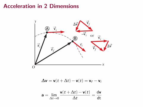
As a particle moves from one point to another along some path, its instanta-neous velocity vector changes from vSi at time ti to vSf at time tf . Knowing the velocity at these points allows us to determine the average acceleration of the particle. The average acceleration aSavg of a particle is defined as the change in its instantaneous velocity vector DvS divided by the time interval Dt during which that change occurs:

aSavg ;DvS

Dt5

vSf 2 vSi

tf 2 ti (4.4)

Because aSavg is the ratio of a vector quantity DvS and a positive scalar quantity Dt, we conclude that average acceleration is a vector quantity directed along DvS. As indicated in Figure 4.3, the direction of DvS is found by adding the vector 2vSi (the negative of vSi) to the vector vSf because, by definition, DvS 5 vSf 2 vSi. Compare Equation 4.4 with Equation 2.9. When the average acceleration of a particle changes during different time inter-vals, it is useful to define its instantaneous acceleration. The instantaneous accel-eration aS is defined as the limiting value of the ratio D vS/Dt as Dt approaches zero:

aS ; limDt S0

DvS

Dt5

d vS

dt (4.5)

In other words, the instantaneous acceleration equals the derivative of the velocity vector with respect to time. Compare Equation 4.5 with Equation 2.10. Various changes can occur when a particle accelerates. First, the magnitude of the velocity vector (the speed) may change with time as in straight-line (one-

Average acceleration X

Instantaneous acceleration X

O

y

x

!!!r1S r2

S r3S

Direction of at vS

As the end point approaches , !t approaches zero and the direction of approaches that of the green line tangent to the curve at .

!rS

As the end point of the path is moved from to to , the respective displacements and corresponding time intervals become smaller and smaller.

" #

!!

!

!

"#

""

"

" " "

x

y

O

vf

or

viS

viS

vfS

vfS

–viS

!vS

!vSriS

rfS

!

"

Figure 4.3 A particle moves from position ! to position ". Its velocity vector changes from vSi to vSf . The vector diagrams at the upper right show two ways of determining the vector DvS from the initial and final velocities.

Figure 4.2 As a particle moves between two points, its average velocity is in the direction of the displacement vector D rS. By defini-tion, the instantaneous velocity at ! is directed along the line tan-gent to the curve at !.

Pitfall Prevention 4.1Vector Addition Although the vec-tor addition discussed in Chapter 3 involves displacement vectors, vec-tor addition can be applied to any type of vector quantity. Figure 4.3, for example, shows the addition of velocity vectors using the graphical approach.

v = lim∆t→0

r(t + ∆t) − r(t)

∆t=

dr

dt

Velocity in 2 Dimensions

Different directions are independent ⇒ differentiate separately!

r = x i + y j

v =dr

dt

=dx

dti +

dy

dtj

v = vx i + vy j

(Differentiation is a linear operation.)

Acceleration in 2 Dimensions

80 Chapter 4 Motion in Two Dimensions

As a particle moves from one point to another along some path, its instanta-neous velocity vector changes from vSi at time ti to vSf at time tf . Knowing the velocity at these points allows us to determine the average acceleration of the particle. The average acceleration aSavg of a particle is defined as the change in its instantaneous velocity vector DvS divided by the time interval Dt during which that change occurs:

aSavg ;DvS

Dt5

vSf 2 vSi

tf 2 ti (4.4)

Because aSavg is the ratio of a vector quantity DvS and a positive scalar quantity Dt, we conclude that average acceleration is a vector quantity directed along DvS. As indicated in Figure 4.3, the direction of DvS is found by adding the vector 2vSi (the negative of vSi) to the vector vSf because, by definition, DvS 5 vSf 2 vSi. Compare Equation 4.4 with Equation 2.9. When the average acceleration of a particle changes during different time inter-vals, it is useful to define its instantaneous acceleration. The instantaneous accel-eration aS is defined as the limiting value of the ratio D vS/Dt as Dt approaches zero:

aS ; limDt S0

DvS

Dt5

d vS

dt (4.5)

In other words, the instantaneous acceleration equals the derivative of the velocity vector with respect to time. Compare Equation 4.5 with Equation 2.10. Various changes can occur when a particle accelerates. First, the magnitude of the velocity vector (the speed) may change with time as in straight-line (one-

Average acceleration X

Instantaneous acceleration X

O

y

x

!!!r1S r2

S r3S

Direction of at vS

As the end point approaches , !t approaches zero and the direction of approaches that of the green line tangent to the curve at .

!rS

As the end point of the path is moved from to to , the respective displacements and corresponding time intervals become smaller and smaller.

" #

!!

!

!

"#

""

"

" " "

x

y

O

vf

or

viS

viS

vfS

vfS

–viS

!vS

!vSriS

rfS

!

"

Figure 4.3 A particle moves from position ! to position ". Its velocity vector changes from vSi to vSf . The vector diagrams at the upper right show two ways of determining the vector DvS from the initial and final velocities.

Figure 4.2 As a particle moves between two points, its average velocity is in the direction of the displacement vector D rS. By defini-tion, the instantaneous velocity at ! is directed along the line tan-gent to the curve at !.

Pitfall Prevention 4.1Vector Addition Although the vec-tor addition discussed in Chapter 3 involves displacement vectors, vec-tor addition can be applied to any type of vector quantity. Figure 4.3, for example, shows the addition of velocity vectors using the graphical approach.

∆v = v(t + ∆t) − v(t) = vf − vi

a = lim∆t→0

v(t + ∆t) − v(t)

∆t=

dv

dt

Kinematic Equations in 2 Dimensions

vf = vi + at


Because the acceleration aS of the particle is assumed constant in this discussion, its components ax and ay also are constants. Therefore, we can model the particle as a particle under constant acceleration independently in each of the two directions and apply the equations of kinematics separately to the x and y components of the velocity vector. Substituting, from Equation 2.13, vxf 5 vxi 1 axt and vyf 5 vyi 1 ayt into Equation 4.7 to determine the final velocity at any time t, we obtain

vSf 5 1vxi 1 axt 2 i 1 1vyi 1 ayt 2 j 5 1vxi i 1 vyi j 2 1 1ax i 1 ay j 2 t vSf 5 vSi 1 aSt (4.8)

This result states that the velocity of a particle at some time t equals the vector sum of its initial velocity vSi at time t 5 0 and the additional velocity aSt acquired at time t as a result of constant acceleration. Equation 4.8 is the vector version of Equation 2.13. Similarly, from Equation 2.16 we know that the x and y coordinates of a particle under constant acceleration are

xf 5 xi 1 vxit 1 12axt 2 yf 5 yi 1 vyit 1 1

2ayt 2

Substituting these expressions into Equation 4.6 (and labeling the final position vector rSf ) gives

rSf 5 1xi 1 vxit 1 12axt 2 2 i 1 1yi 1 vyit 1 1

2ayt 2 2 j 5 1xi i 1 yi j 2 1 1vxi i 1 vyi j 2 t 1 1

2 1ax i 1 ay j 2 t 2

rSf 5 rSi 1 vSit 1 12 aSt 2 (4.9)

which is the vector version of Equation 2.16. Equation 4.9 tells us that the position vector rSf of a particle is the vector sum of the original position rSi, a displacement vSi t arising from the initial velocity of the particle, and a displacement 1

2 aSt 2 result-ing from the constant acceleration of the particle. We can consider Equations 4.8 and 4.9 to be the mathematical representation of a two-dimensional version of the particle under constant acceleration model. Graphical representations of Equations 4.8 and 4.9 are shown in Figure 4.5. The components of the position and velocity vectors are also illustrated in the figure. Notice from Figure 4.5a that vSf is generally not along the direction of either vSi or aS because the relationship between these quantities is a vector expression. For the same reason, from Figure 4.5b we see that rSf is generally not along the direction of rSi, vSi, or aS. Finally, notice that vSf and rSf are generally not in the same direction.

Velocity vector as Wa function of time for a particle under constant

acceleration in two dimensions

Position vector as a function of time for a particle under constant


Figure 4.5 Vector representa-tions and components of (a) the velocity and (b) the position of a particle under constant accelera-tion in two dimensions.

y

x

ayt

vyf

vyi

t

vxi axt

vxf

y

x

yf

yi

it

vxit

xf

ayt21

2

vyit

t212

axt21

2xi

viS vi

S

vfS

riS

rfSaS aS

a b

Equating x-components (i-components):

vx = vx ,i + ax t

Equating y -components (j-components):

vy = vy ,i + ay t


vf = vi + at

vf = (vx ,i i + vy ,i j) + (ax i + ay j)t

vx i + vy j = (vx ,i + ax t)i + (vy ,i + ay t)j


Because the acceleration aS of the particle is assumed constant in this discussion, its components ax and ay also are constants. Therefore, we can model the particle as a particle under constant acceleration independently in each of the two directions and apply the equations of kinematics separately to the x and y components of the velocity vector. Substituting, from Equation 2.13, vxf 5 vxi 1 axt and vyf 5 vyi 1 ayt into Equation 4.7 to determine the final velocity at any time t, we obtain

vSf 5 1vxi 1 axt 2 i 1 1vyi 1 ayt 2 j 5 1vxi i 1 vyi j 2 1 1ax i 1 ay j 2 t vSf 5 vSi 1 aSt (4.8)

This result states that the velocity of a particle at some time t equals the vector sum of its initial velocity vSi at time t 5 0 and the additional velocity aSt acquired at time t as a result of constant acceleration. Equation 4.8 is the vector version of Equation 2.13. Similarly, from Equation 2.16 we know that the x and y coordinates of a particle under constant acceleration are

xf 5 xi 1 vxit 1 12axt 2 yf 5 yi 1 vyit 1 1

2ayt 2

Substituting these expressions into Equation 4.6 (and labeling the final position vector rSf ) gives

rSf 5 1xi 1 vxit 1 12axt 2 2 i 1 1yi 1 vyit 1 1

2ayt 2 2 j 5 1xi i 1 yi j 2 1 1vxi i 1 vyi j 2 t 1 1

2 1ax i 1 ay j 2 t 2

rSf 5 rSi 1 vSit 1 12 aSt 2 (4.9)

which is the vector version of Equation 2.16. Equation 4.9 tells us that the position vector rSf of a particle is the vector sum of the original position rSi, a displacement vSi t arising from the initial velocity of the particle, and a displacement 1

2 aSt 2 result-ing from the constant acceleration of the particle. We can consider Equations 4.8 and 4.9 to be the mathematical representation of a two-dimensional version of the particle under constant acceleration model. Graphical representations of Equations 4.8 and 4.9 are shown in Figure 4.5. The components of the position and velocity vectors are also illustrated in the figure. Notice from Figure 4.5a that vSf is generally not along the direction of either vSi or aS because the relationship between these quantities is a vector expression. For the same reason, from Figure 4.5b we see that rSf is generally not along the direction of rSi, vSi, or aS. Finally, notice that vSf and rSf are generally not in the same direction.

Velocity vector as Wa function of time for a particle under constant


Position vector as a function of time for a particle under constant


Figure 4.5 Vector representa-tions and components of (a) the velocity and (b) the position of a particle under constant accelera-tion in two dimensions.

y

x

ayt

vyf

vyi

t

vxi axt

vxf

y

x

yf

yi

it

vxit

xf

ayt21

2

vyit

t212

axt21

2xi

viS vi

S

vfS

riS

rfSaS aS

a bEquating x-components (i-components):

vx = vx ,i + ax t

Equating y -components (j-components):

vy = vy ,i + ay t


The other kinematics equations work basically the same way asvf = vi + at.

These are also vector equations and the components add up thesame way:

∆r = vi t +1

2at2

∆r =1

2(vi + vf )t

This one is a scalar equation:

v2f = v2

i + 2a ·∆r

(Why is it a scalar equation?)


The other kinematics equations work basically the same way asvf = vi + at.These are also vector equations and the components add up thesame way:

∆r = vi t +1

2at2

∆r =1

2(vi + vf )t

This one is a scalar equation:

v2f = v2

i + 2a ·∆r

(Why is it a scalar equation?)

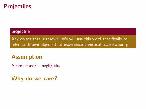
Projectiles

projectile

Any object that is thrown. We will use this word specifically torefer to thrown objects that experience a vertical acceleration g .

Assumption

Air resistance is negligible.

Why do we care?

Projectilesprojectile

Any object that is thrown. We will use this word specifically torefer to thrown objects that experience a vertical acceleration g .

Assumption

Air resistance is negligible.

Why do we care?

Projectile Velocity 4.3 Projectile Motion 85

Figure 4.7 The parabolic path of a projectile that leaves the ori-gin with a velocity vSi . The velocity vector vS changes with time in both magnitude and direction. This change is the result of accel-eration aS 5 gS in the negative y direction.

f

x

(x,y)it

O

y

t212 gS

rS

vS

Figure 4.8 The position vector rSf of a projectile launched from the origin whose initial velocity at the origin is vSi . The vector vSit would be the displacement of the projectile if gravity were absent, and the vector 12 gSt 2 is its vertical displacement from a straight-line path due to its downward gravita-tional acceleration.

R

x

y

h

i

vy ! 0

i

O

u

vS!

"

!

Figure 4.9 A projectile launched over a flat surface from the origin at ti 5 0 with an initial velocity vSi . The maximum height of the projectile is h, and the horizontal range is R. At !, the peak of the trajectory, the particle has coordi-nates (R/2, h).

In Section 4.2, we stated that two-dimensional motion with constant accelera-tion can be analyzed as a combination of two independent motions in the x and y directions, with accelerations ax and ay. Projectile motion can also be handled in this way, with acceleration ax 5 0 in the x direction and a constant acceleration ay 5 2g in the y direction. Therefore, when solving projectile motion problems, use two analysis models: (1) the particle under constant velocity in the horizontal direction (Eq. 2.7):

xf 5 xi 1 vxit

and (2) the particle under constant acceleration in the vertical direction (Eqs. 2.13–2.17 with x changed to y and ay = –g):

vyf 5 vyi 2 gt

vy,avg 5vyi 1 vyf

2

yf 5 yi 1 12 1vyi 1 vyf 2 t

yf 5 yi 1 vyit 2 12gt 2

vyf2 5 vyi

2 2 2g 1 yf 2 yi 2

The horizontal and vertical components of a projectile’s motion are completely independent of each other and can be handled separately, with time t as the com-mon variable for both components.

Q uick Quiz 4.2 (i) As a projectile thrown upward moves in its parabolic path (such as in Fig. 4.8), at what point along its path are the velocity and accelera-tion vectors for the projectile perpendicular to each other? (a) nowhere (b) the highest point (c) the launch point (ii) From the same choices, at what point are the velocity and acceleration vectors for the projectile parallel to each other?

Horizontal Range and Maximum Height of a ProjectileBefore embarking on some examples, let us consider a special case of projectile motion that occurs often. Assume a projectile is launched from the origin at ti 5 0 with a positive vyi component as shown in Figure 4.9 and returns to the same hori-zontal level. This situation is common in sports, where baseballs, footballs, and golf balls often land at the same level from which they were launched. Two points in this motion are especially interesting to analyze: the peak point !, which has Cartesian coordinates (R/2, h), and the point ", which has coordinates (R , 0). The distance R is called the horizontal range of the projectile, and the distance h is its maximum height. Let us find h and R mathematically in terms of vi, ui, and g.

xvxi

vxi

vy

vy ! 0

vxi

vy

ivy

vy

i

vxi

y

i

i

u

uu

u

The y component of velocity is zero at the peak of the path.

The x component of velocity remains constant because there is no acceleration in the x direction.

vS

The projectile is launched with initial velocity vi.

S

vSvS

vS

vS

gS

!

"

# $

%

"#

$

%

Projectile Velocity 4.3 Projectile Motion 85


f

x

(x,y)it

O

y

t212 gS

rS

vS


R

x

y

h

i

vy ! 0

i

O

u

vS!

"

!



xf 5 xi 1 vxit


vyf 5 vyi 2 gt

vy,avg 5vyi 1 vyf

2



vyf2 5 vyi

2 2 2g 1 yf 2 yi 2




xvxi

vxi

vy

vy ! 0

vxi

vy

ivy

vy

i

vxi

y

i

i

u

uu

u



vS


S

vSvS

vS

vS

gS

!

"

# $

%

"#

$

%

← But the yaccelerationis not zero!

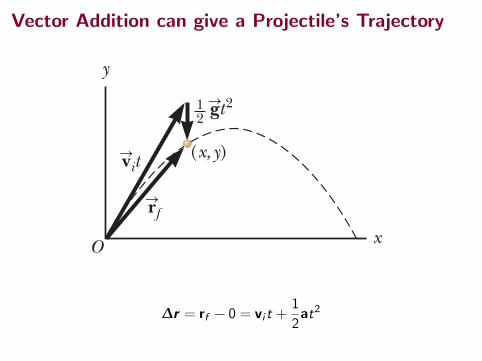
Vector Addition can give a Projectile’s Trajectory

4.3 Projectile Motion 85


f

x

(x,y)it

O

y

t212 gS

rS

vS


R

x

y

h

i

vy ! 0

i

O

u

vS!

"

!



xf 5 xi 1 vxit


vyf 5 vyi 2 gt

vy,avg 5vyi 1 vyf

2



vyf2 5 vyi

2 2 2g 1 yf 2 yi 2




xvxi

vxi

vy

vy ! 0

vxi

vy

ivy

vy

i

vxi

y

i

i

u

uu

u



vS


S

vSvS

vS

vS

gS

!

"

# $

%

"#

$

%

∆r = rf − 0 = vi t +1

2at2

Height of a Projectile

How can we find the maximum height that a projectile reaches?

c



f

x

(x,y)it

O

y

t212 gS

rS

vS


R

x

y

h

i

vy ! 0

i

O

u

vS!

"

!



xf 5 xi 1 vxit


vyf 5 vyi 2 gt

vy,avg 5vyi 1 vyf

2



vyf2 5 vyi

2 2 2g 1 yf 2 yi 2




xvxi

vxi

vy

vy ! 0

vxi

vy

ivy

vy

i

vxi

y

i

i

u

uu

u



vS


S

vSvS

vS

vS

gS

!

"

# $

%

"#

$

%

Find the height when vy = 0.

v2f ,y = v2

i ,y − 2g∆y

0 = v2y ,i − 2gh

h =v2y ,i

2g

In the diagram, vy ,i = vi sin θ.

h =v2i sin2 θ

2g

Time of Flight of a Projectile

time of flight

The time from launch to when projectile hits the ground.

How can we find the time of flight of a projectile?



f

x

(x,y)it

O

y

t212 gS

rS

vS


R

x

y

h

i

vy ! 0

i

O

u

vS!

"

!



xf 5 xi 1 vxit


vyf 5 vyi 2 gt

vy,avg 5vyi 1 vyf

2



vyf2 5 vyi

2 2 2g 1 yf 2 yi 2




xvxi

vxi

vy

vy ! 0

vxi

vy

ivy

vy

i

vxi

y

i

i

u

uu

u



vS


S

vSvS

vS

vS

gS

!

"

# $

%

"#

$

%

Assuming that it is launched from the ground and lands on theground at the same height...


Use symmetry! A parabola is always symmetric about a linethrough it’s vertex.



1 That means the time to go up and return to the ground arethe same. Find the time to reach the vy = 0 point, (“thalf”)then multiply by two.




2 Or, notice that just before striking the ground, vy ,f = −vy ,i .





3 Or, notice that just when striking the ground, ∆y = 0.





1.vy ,f = vy ,i + ay t

0 = vi sin θ− gthalf

thalf =vi sin θ

g

tflight =2vi sin θ

g






0 = vi sin θ− gthalf

thalf =vi sin θ

g

tflight =2vi sin θ

g


−vi sin θ = vi sin θ− gt

t =2vi sin θ

g

tflight =2vi sin θ

g


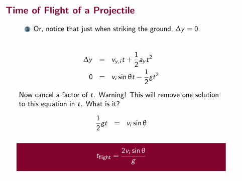
3 Or, notice that just when striking the ground, ∆y = 0.

∆y = vy ,i t +1

2ay t

2

0 = vi sin θt −1

2gt2

Now cancel a factor of t. Warning! This will remove one solutionto this equation in t. What is it?

1

2gt = vi sin θ

tflight =2vi sin θ

g

Time of Flight of a ProjectileQuick Quiz 4.31 Rank the launch angles for the five paths in thefigure with respect to time of flight from the shortest time of flightto the longest. (Assume the magnitude vi remains the same.)


We can determine h by noting that at the peak vy! 5 0. Therefore, from the particle under constant acceleration model, we can use the y direction version of Equation 2.13 to determine the time t! at which the projectile reaches the peak:

vyf 5 vyi 2 gt S 0 5 vi sin ui 2 gt !

t ! 5vi sin ui

g

Substituting this expression for t! into the y direction version of Equation 2.16 and replacing yf 5 y! with h, we obtain an expression for h in terms of the magni-tude and direction of the initial velocity vector:

yf 5 yi 1 vyit 2 12gt 2 S h 5 1vi sin ui 2 vi sin ui

g 2 12g avi sin ui

g b2

h 5vi

2 sin2 ui

2g (4.12)

The range R is the horizontal position of the projectile at a time that is twice the time at which it reaches its peak, that is, at time t" 5 2t!. Using the particle under constant velocity model, noting that vxi 5 vx" 5 vi cos ui, and setting x" 5 R at t 5 2t!, we find that

xf 5 xi 1 vxit S R 5 vxit " 5 1vi cos ui 22t !

5 1vi cos ui 2 2vi sin ui

g 52vi

2 sin ui cos ui

g

Using the identity sin 2u 5 2 sin u cos u (see Appendix B.4), we can write R in the more compact form

R 5vi

2 sin 2ui

g (4.13)

The maximum value of R from Equation 4.13 is Rmax 5 vi2/g . This result makes

sense because the maximum value of sin 2ui is 1, which occurs when 2ui 5 90°. Therefore, R is a maximum when ui 5 45°. Figure 4.10 illustrates various trajectories for a projectile having a given initial speed but launched at different angles. As you can see, the range is a maximum for ui 5 45°. In addition, for any ui other than 45°, a point having Cartesian coordi-nates (R, 0) can be reached by using either one of two complementary values of ui, such as 75° and 15°. Of course, the maximum height and time of flight for one of these values of ui are different from the maximum height and time of flight for the complementary value.

Q uick Quiz 4.3 Rank the launch angles for the five paths in Figure 4.10 with respect to time of flight from the shortest time of flight to the longest.

50

100

150y (m)

x (m)

75!

60!

45!

30!

15!

vi " 50 m/s

50 100 150 200 250

Complementary values of the initial angle ui result in the same value of R.

Figure 4.10 A projectile launched over a flat surface from the origin with an initial speed of 50 m/s at various angles of projection.

Pitfall Prevention 4.3The Range Equation Equation 4.13 is useful for calculating R only for a symmetric path as shown in Figure 4.10. If the path is not sym-metric, do not use this equation. The particle under constant velocity and particle under constant accel-eration models are the important starting points because they give the position and velocity compo-nents of any projectile moving with constant acceleration in two dimensions at any time t.

A 15◦, 30◦, 45◦, 60◦, 75◦

B 45◦, 30◦, 60◦, 15◦, 75◦

C 15◦, 75◦, 30◦, 60◦, 45◦

D 75◦, 60◦, 45◦, 30◦, 15◦

1Page 86, Serway & Jewett

Time of Flight of a ProjectileQuick Quiz 4.31 Rank the launch angles for the five paths in thefigure with respect to time of flight from the shortest time of flightto the longest. (Assume the magnitude vi remains the same.)


We can determine h by noting that at the peak vy! 5 0. Therefore, from the particle under constant acceleration model, we can use the y direction version of Equation 2.13 to determine the time t! at which the projectile reaches the peak:

vyf 5 vyi 2 gt S 0 5 vi sin ui 2 gt !

t ! 5vi sin ui

g

Substituting this expression for t! into the y direction version of Equation 2.16 and replacing yf 5 y! with h, we obtain an expression for h in terms of the magni-tude and direction of the initial velocity vector:

yf 5 yi 1 vyit 2 12gt 2 S h 5 1vi sin ui 2 vi sin ui

g 2 12g avi sin ui

g b2

h 5vi

2 sin2 ui

2g (4.12)

The range R is the horizontal position of the projectile at a time that is twice the time at which it reaches its peak, that is, at time t" 5 2t!. Using the particle under constant velocity model, noting that vxi 5 vx" 5 vi cos ui, and setting x" 5 R at t 5 2t!, we find that

xf 5 xi 1 vxit S R 5 vxit " 5 1vi cos ui 22t !

5 1vi cos ui 2 2vi sin ui

g 52vi

2 sin ui cos ui

g

Using the identity sin 2u 5 2 sin u cos u (see Appendix B.4), we can write R in the more compact form

R 5vi

2 sin 2ui

g (4.13)

The maximum value of R from Equation 4.13 is Rmax 5 vi2/g . This result makes

sense because the maximum value of sin 2ui is 1, which occurs when 2ui 5 90°. Therefore, R is a maximum when ui 5 45°. Figure 4.10 illustrates various trajectories for a projectile having a given initial speed but launched at different angles. As you can see, the range is a maximum for ui 5 45°. In addition, for any ui other than 45°, a point having Cartesian coordi-nates (R, 0) can be reached by using either one of two complementary values of ui, such as 75° and 15°. Of course, the maximum height and time of flight for one of these values of ui are different from the maximum height and time of flight for the complementary value.

Q uick Quiz 4.3 Rank the launch angles for the five paths in Figure 4.10 with respect to time of flight from the shortest time of flight to the longest.

50

100

150y (m)

x (m)

75!

60!

45!

30!

15!

vi " 50 m/s

50 100 150 200 250

Complementary values of the initial angle ui result in the same value of R.

Figure 4.10 A projectile launched over a flat surface from the origin with an initial speed of 50 m/s at various angles of projection.

Pitfall Prevention 4.3The Range Equation Equation 4.13 is useful for calculating R only for a symmetric path as shown in Figure 4.10. If the path is not sym-metric, do not use this equation. The particle under constant velocity and particle under constant accel-eration models are the important starting points because they give the position and velocity compo-nents of any projectile moving with constant acceleration in two dimensions at any time t.

A 15◦, 30◦, 45◦, 60◦, 75◦←B 45◦, 30◦, 60◦, 15◦, 75◦

C 15◦, 75◦, 30◦, 60◦, 45◦

D 75◦, 60◦, 45◦, 30◦, 15◦

1Page 86, Serway & Jewett

Summary

• projectile motion

• height, range of a projectile

• trajectory equation for a projectile

Collected Homework! due Friday, Oct 6.

(Uncollected) Homework Serway & Jewett,

• Ch 4 Work through example 4.5 (Ski Jumper) on page 90.Understand it.

• Ch 4, onward from page 102. Probs: 7, 11, 15, 21, 29, 37, 39

• Read Ch 1-4, if you haven’t already.

2D Motion Projectile Motion - De Anza...

Documents

Transcript of 2D Motion Projectile Motion - De Anza...