iii

Student Guide for

Elementary Business Statistics

Dean H Fearn

Elliot Nebenzahl

Maurice Geraghty

2003

iv

OUTLINE

I. Introduction 1

A. What Does the Term ‘Statistics’ Mean? B. Introductory Terms including Population, Parameter, Sample, Statistic C. Example of ‘Inferential Statistics’, ‘Probability’, ‘Descriptive Statistics’ D. Loading Statistical Software in Microsoft Excel

II. Graphs and Tables 3

A. Stem and Leaf Plot B. Grouping Data C. Frequency, Relative Frequency, %, Cumulative Frequency, Plus More D. Histogram E. Problems F. Using Excel to Make Frequency Distributions and Histograms

III. Measures of Central tendency 10

A. Mean, Median, Mode B. Symmetry versus Skewness C. Problems

IV. Measures of Variation (or Dispersion) 14

A. Range, Variance, Standard deviation B. Empirical Rule C. Percentiles, Quartiles, Box-Plots D. Problems E. Using Excel to find Descriptive Statistics

V. Probability 23

A. Empirical Definition versus Classical (or Counting) Definition B. Combinations C. Lotto-Like Problems D. Two-way Table Problems E. Qualitative versus Quantitative Variables & Discrete versus Continuous

Variables F. Problems

VI. Discrete Probability Distributions 37

v

A. Introduction B. Binomial C. Population Mean μ and Population Standard deviation σ for a Discrete

Random Variable D. Hypergeometric (≡ Lotto-Like) Distribution E. Poisson F. Problems

G. Using Excel to Create Probability Distribution Tables VII. Continuous Probability Distributions 52

A. Normal B. Normal Approximation to the Binomial C. Problems D. Continuous Distributions in General

E. Using Excel to find Normal Probabilities and Percentiles VIII. Background for Inference 74 IX. One Sample Inference: Quantitative Data 76

A. Confidence Intervals for a Population Mean: Large & Small Sample B. Hypothesis Testing for a Population Mean: Large & Small Sample C. Using Excel for One Sample Inference

X. One Sample Inference: Qualitative Data 95 XI. Two Sample Inference: Quantitative Data 102 A. Large & Small Samples B. Problems C. Using Excel for Two Sample Inference XII. Regression and Correlation 112

A. Pearson’s Correlation Coefficient B. Least-Squares Line C. Coefficient of Determination D. Inference on the population correlation E. Problems F. Using Microsoft Excel: Instruction plus Problems G. Applications Plus Problems Relating to Capital Asset Pricing Model and

Autoregression XIII. Multiple Regression 130

vi

XIV. Tables 144

A. Cumulative Standard Normal Tables B. t-tables

XV. Appendix 147 A. Graphical Description of Menus for the Step-wise Routine of Minitab B. Graphical Description of Menus for Multiple Regression in Excel

vii

PREFACE

The purpose of writing this Student Guide is to tailor its organization and content

plus the problems assigned, to the course lectures. The authors feel comfortable with the material as presented in this guide. It contains a concise treatment of a number of topics that one would want to cover in a beginning one-quarter course in business statistics. In terms of the material presented, this book is reasonably self-contained but course instructors should feel free to add additional material as handouts as they see fit. However, we hope in the future to supplement the workbook with cumulative and exact-probability binomial tables, and cumulative and exact probability Poisson tables; these could then be obtained at a web address.

The advantage of this short book is that the cost to the students will be minimal when compared to the cost of most textbooks. We have instructions in the workbook for performing simple and multiple linear regression with Excel; earlier sections include Excel instructions for much of the earlier material in the book. Also, The simple regression chapter includes material on the ‘Capital Asset Pricing Model’ and ‘Autoregression’. Finally the multiple regression chapter has a brief discussion on some routines found in the statistical package Minitab for determining a reasonable prediction equation.

.

1

I. Introduction

A. What does the term ‘Statistics’ mean?

Statistics is the science of dealing with data. This includes:

1. Deciding what data to obtain. 2. Quantifying and describing the data. 3. Using the data to make inferences.

B. Introductory Terms including Population, Parameter, Sample, Statistic

A population consists of all items of interest.

A sample is the group of observed items selected from the population. The goal of statistics is to use the information gathered from the sample to describe the sample (‘Descriptive Statistics’) and to make estimates (or draw conclusions) about the whole population based on the description of the sample (‘Inferential Statistics’).

A particular item in a population or sample is called an element or member of the population or sample.

A variable is a measurable or observable characteristic of the elements of a population or sample. The values of a variable differ among these elements.

The value of a variable is called a measurement or observation.

The collection of measurements is called the data set.

The distribution of the data refers to the pattern of the measurements that comprise the data.

A quantity describing the population is called a parameter.

A quantity describing the sample is called a statistic.

C. Example of ‘Inferential Statistics’, ‘Probability’, ‘Descriptive Statistics’

We are interested in the amount of recall for TV viewers who watch a certain advertisement delivered by a famous personality. We randomly select 25 viewers, have them watch the advertisement and then test them on their recall of the Ad on a scale from 0 to 10, with the higher the number the greater the recall. The population could be the recall values for all viewers of the commercial, with a possible parameter being the population average recall value. The sample consists of the 25 recall values of the selected viewers; a random sample from the population would mean that all groups of 25 viewers would have an equal chance of being chosen from the population. A possible statistic could then be the sample average recall value based on the 25 scores in the sample.

2

The latter part of the course deals with inferential statistics, whereby one may draw conclusions from the sample about the entire population. An example of an inference based on a sample is “ from the average recall value of 7.48, one concludes with 95% confidence the population average recall is between 6.48 and 8.48.” The reason that we cannot be 100% confident is that the entire information in the population is not readily available to us. When we talk about 95% confidence, there is a 95% chance that our interval contains the population average and a 5% chance that it does not.

The ideas relating to the chance of an event occurring or not, relate to the area of Probability and this occupies the middle part of the course. The beginning part of the course merely deals with methods of making the sample data look nice, referred to as descriptive statistics. The ways of doing this are by means of tables, graphs, and various summary statistics.

D. Loading Statistical Software in Microsoft Excel

Many of the applications and problems in this text can be run in Excel’s standard programs and functions and in it’s Data Analysis ToolPak add-in. Since Analysis ToolPak is not normally functional with the standard instillation of Microsoft Office, use the following procedure to install the ToolPak:

Start up Microsoft Excel. Click the Menu Item Tools>Addins.

Click the box next to “Analysis ToolPak” until a checkmark appears. The program may prompt you for Microsoft Office CD.

The Menu Item Tools>Data Analysis should now appear on the menu.

3

II. Graphs and Tables

A. Stem and Leaf Plot

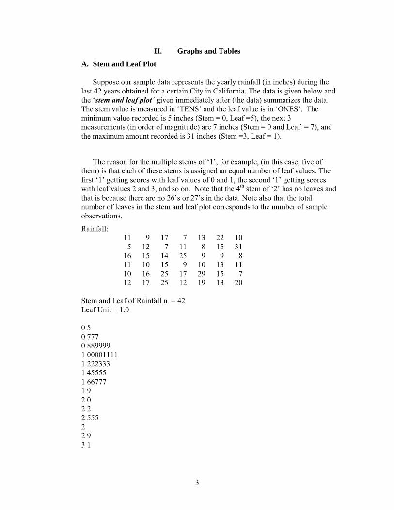
Suppose our sample data represents the yearly rainfall (in inches) during the last 42 years obtained for a certain City in California. The data is given below and the ‘stem and leaf plot’ given immediately after (the data) summarizes the data. The stem value is measured in ‘TENS’ and the leaf value is in ‘ONES’. The minimum value recorded is 5 inches (Stem = 0, Leaf =5), the next 3 measurements (in order of magnitude) are 7 inches (Stem = 0 and Leaf = 7), and the maximum amount recorded is 31 inches (Stem =3, Leaf = 1).

The reason for the multiple stems of ‘1’, for example, (in this case, five of them) is that each of these stems is assigned an equal number of leaf values. The first ‘1’ getting scores with leaf values of 0 and 1, the second ‘1’ getting scores with leaf values 2 and 3, and so on. Note that the 4th stem of ‘2’ has no leaves and that is because there are no 26’s or 27’s in the data. Note also that the total number of leaves in the stem and leaf plot corresponds to the number of sample observations.

Rainfall: 11 9 17 7 13 22 105 12 7 11 8 15 31

16 15 14 25 9 9 811 10 15 9 10 13 1110 16 25 17 29 15 712 17 25 12 19 13 20

Stem and Leaf of Rainfall n = 42 Leaf Unit = 1.0

0 5 0 777 0 889999 1 00001111 1 222333 1 45555 1 66777 1 9 2 0 2 2 2 555 2 2 9 3 1

4

B. Grouping Data

Suppose that we wanted to group the above rainfall data into 4 intervals, all having an equal width. Suppose also that we wanted to begin the smallest interval with a score of 4; note that this starting score cannot be bigger than the min (minimum), since then the min will fail to be included in any of the intervals. To decide on the common width of the intervals, call it the class width w, set w = (max(imum) – starting score)/(# of desired intervals) and then round the answer up to the next whole number (when our data is measured in whole numbers).

For this example, w = (31-4)/4 = 6.75 ≈ 7 and thus the common width = 7.

We then use the intervals 4- under 11(= 4+7), 11- under 18 (= 11+7), 18- under 25 and 25- under 32 and group our data according to these intervals. ‘Under 11’ means less than 11 and does not include a score of ‘11’ and so on. Equivalently, one could have decided to group the data into intervals of width (also, called length) 7, with the first interval starting at 4 (or since the first interval would have been 4- under 11), it could have been stated as the starting midpoint being 7.5 (= (4+11)/2).

C. Frequency, Relative Frequency, %, Cumulative Frequency, Plus More

For each of the intervals given above, we count how many of the 42 observations fall into the interval and this gives us the ‘Frequency’ f or count for the interval resulting in

Interval Frequency

f Relative

Freq. nf

% 100n

f Cum Freq Midpoint

m Density

wnf

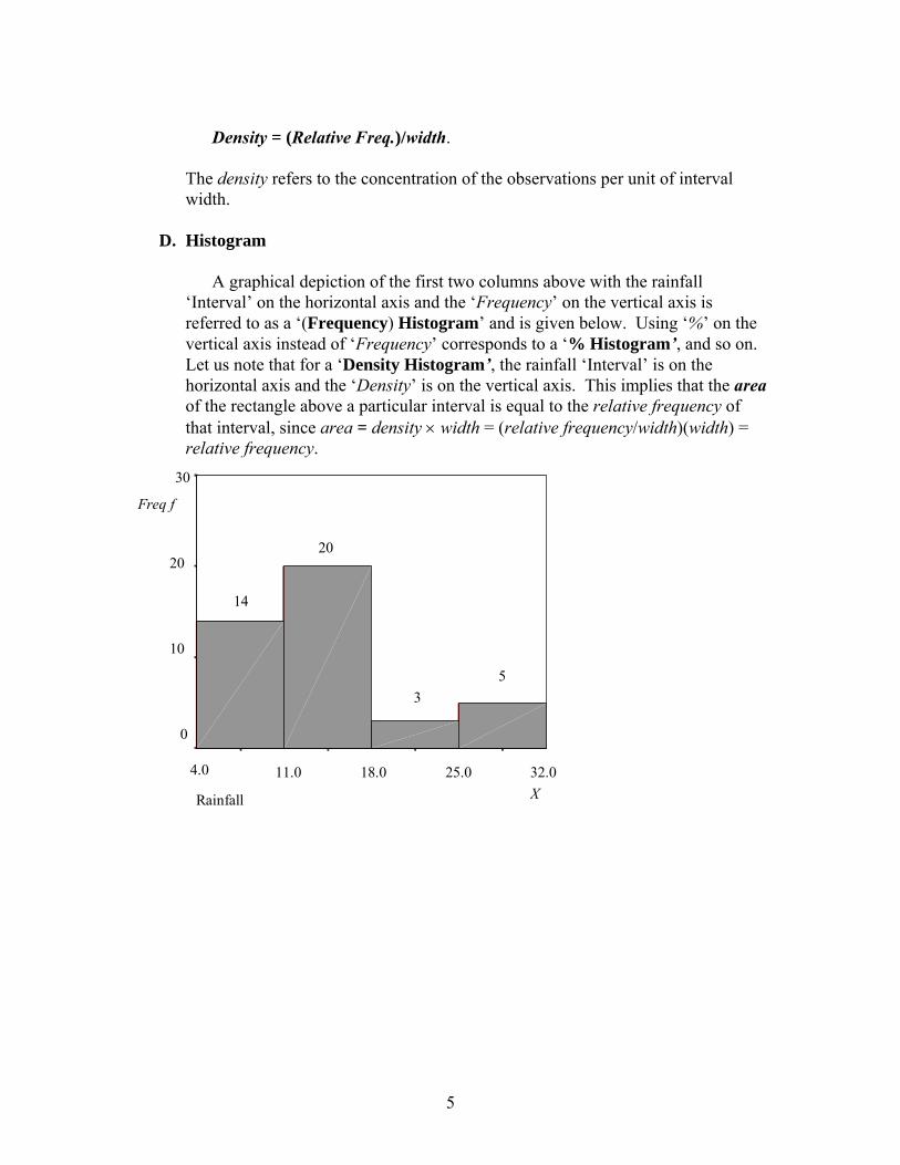
4-under 11 14 14/42 = .33 33 14 7.5 .0471411-under 18 20 20/42 = .48 48 14+20 = 34 14.5 .0685718-under 25 3 3/42 = .07 7 34+3= 37 21.5 .0100025-under 32 5 5/42 = .12 12 42 28.5 .01714

Total 42== ∑ fn 00.1=∑ nf

Thus 14 of the observations are included in the first interval and so on. The

‘Relative Frequency’ of an in interval is the proportion of the observations in an interval, i.e., Relative Freq. = n

f ; the ‘%’ of the cases in an interval is simply

nf 100. Finally the ‘Cumulative Frequency’ of an interval is the count for the

interval itself, added to the counts of other intervals that are numerically smaller than this interval; thus the ‘Cum Freq.’ value for the interval 18-under 25 corresponds to the number of observations under 25. The ‘Midpoint’ (say, m) of an interval is defined by m = (lower value + upper value)/2; thus for the 1st interval, m = (4+11)/2 = 7.5. The ‘Density’ of an interval is defined by

5

Density = (Relative Freq.)/width.

The density refers to the concentration of the observations per unit of interval width.

D. Histogram

A graphical depiction of the first two columns above with the rainfall ‘Interval’ on the horizontal axis and the ‘Frequency’ on the vertical axis is referred to as a ‘(Frequency) Histogram’ and is given below. Using ‘%’ on the vertical axis instead of ‘Frequency’ corresponds to a ‘% Histogram’, and so on. Let us note that for a ‘Density Histogram’, the rainfall ‘Interval’ is on the horizontal axis and the ‘Density’ is on the vertical axis. This implies that the area of the rectangle above a particular interval is equal to the relative frequency of that interval, since area = density × width = (relative frequency/width)(width) = relative frequency.

Rainfall

30

20

10

0

11.0 18.04.0 25.0 32.0X

14

20

Freq f

3

20

5

6

E. Problems

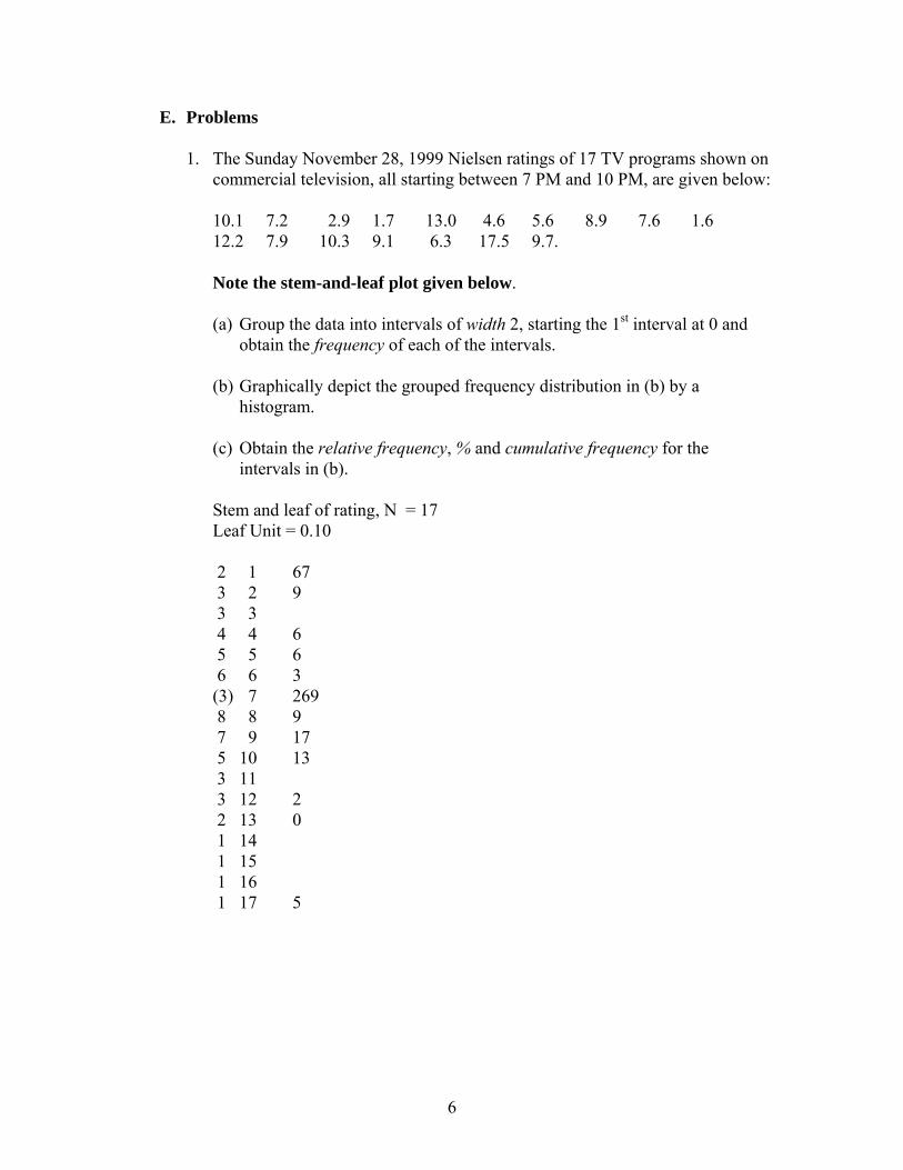
1. The Sunday November 28, 1999 Nielsen ratings of 17 TV programs shown on commercial television, all starting between 7 PM and 10 PM, are given below:

10.1 7.2 2.9 1.7 13.0 4.6 5.6 8.9 7.6 1.6 12.2 7.9 10.3 9.1 6.3 17.5 9.7. Note the stem-and-leaf plot given below. (a) Group the data into intervals of width 2, starting the 1st interval at 0 and

obtain the frequency of each of the intervals.

(b) Graphically depict the grouped frequency distribution in (b) by a histogram.

(c) Obtain the relative frequency, % and cumulative frequency for the

intervals in (b).

Stem and leaf of rating, N = 17 Leaf Unit = 0.10

2 1 67 3 2 9 3 3 4 4 6 5 5 6 6 6 3 (3) 7 269 8 8 9 7 9 17 5 10 13 3 11 3 12 2 2 13 0 1 14 1 15 1 16 1 17 5

7

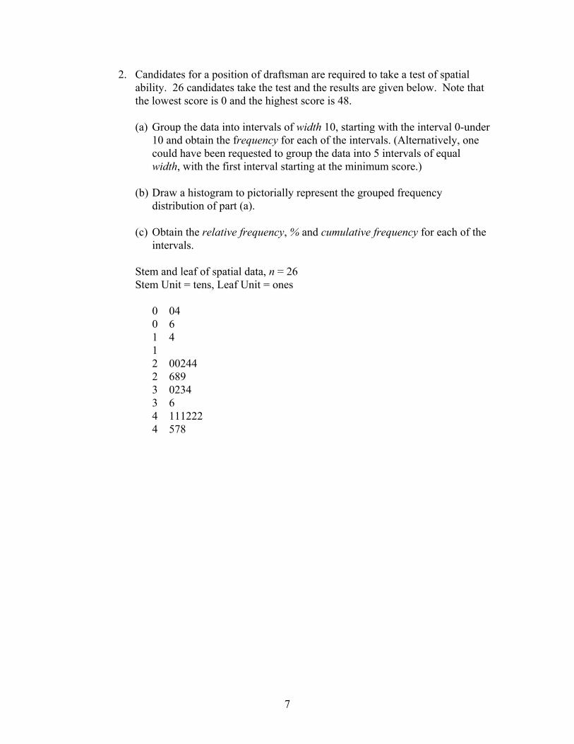
2. Candidates for a position of draftsman are required to take a test of spatial ability. 26 candidates take the test and the results are given below. Note that the lowest score is 0 and the highest score is 48.

(a) Group the data into intervals of width 10, starting with the interval 0-under

10 and obtain the frequency for each of the intervals. (Alternatively, one could have been requested to group the data into 5 intervals of equal width, with the first interval starting at the minimum score.)

(b) Draw a histogram to pictorially represent the grouped frequency

distribution of part (a). (c) Obtain the relative frequency, % and cumulative frequency for each of the

intervals.

Stem and leaf of spatial data, n = 26 Stem Unit = tens, Leaf Unit = ones

0 04 0 6 1 4 1 2 00244 2 689 3 0234 3 6 4 111222 4 578

8

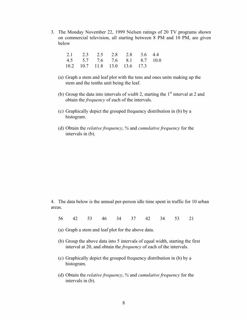
3. The Monday November 22, 1999 Nielsen ratings of 20 TV programs shown on commercial television, all starting between 8 PM and 10 PM, are given below

2.1 2.3 2.5 2.8 2.8 3.6 4.4 4.5 5.7 7.6 7.6 8.1 8.7 10.0 10.2 10.7 11.8 13.0 13.6 17.3

(a) Graph a stem and leaf plot with the tens and ones units making up the

stem and the tenths unit being the leaf. (b) Group the data into intervals of width 2, starting the 1st interval at 2 and

obtain the frequency of each of the intervals. (c) Graphically depict the grouped frequency distribution in (b) by a

histogram. (d) Obtain the relative frequency, % and cumulative frequency for the

intervals in (b).

4. The data below is the annual per-person idle time spent in traffic for 10 urban areas.

56 42 53 46 34 37 42 34 53 21 (a) Graph a stem and leaf plot for the above data.

(b) Group the above data into 5 intervals of equal width, starting the first interval at 20, and obtain the frequency of each of the intervals.

(c) Graphically depict the grouped frequency distribution in (b) by a

histogram. (d) Obtain the relative frequency, % and cumulative frequency for the

intervals in (b).

9

F. Using Excel to Make Frequency Distributions and Histograms

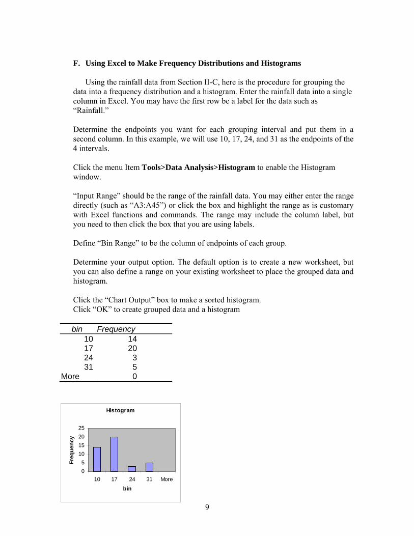
Using the rainfall data from Section II-C, here is the procedure for grouping the

data into a frequency distribution and a histogram. Enter the rainfall data into a single column in Excel. You may have the first row be a label for the data such as “Rainfall.”

Determine the endpoints you want for each grouping interval and put them in a

second column. In this example, we will use 10, 17, 24, and 31 as the endpoints of the 4 intervals.

Click the menu Item Tools>Data Analysis>Histogram to enable the Histogram window.

“Input Range” should be the range of the rainfall data. You may either enter the range

directly (such as “A3:A45”) or click the box and highlight the range as is customary with Excel functions and commands. The range may include the column label, but you need to then click the box that you are using labels.

Define “Bin Range” to be the column of endpoints of each group.

Determine your output option. The default option is to create a new worksheet, but you can also define a range on your existing worksheet to place the grouped data and histogram.

Click the “Chart Output” box to make a sorted histogram.

Click “OK” to create grouped data and a histogram bin Frequency

10 14 17 20 24 3 31 5

More 0

Histogram

05

10152025

10 17 24 31 More

bin

Freq

uenc

y

10

III. Measures of Central tendency

A. Mean, Median, Mode

The 3 statistics mean, median and mode, all measure a ‘typical’ score. The (sample) mean or average denoted by x (x-bar) is defined by x = n

x∑ , where

∑ x denotes the sum of all the observations in the sample. For the earlier rainfall data, ∑ x = 11+9+…+13 = 590 and since n = 42, x = 42

590 = 14.048. The sample median is a number, which is at least as large as half, or more of

the sample’s scores, but which is not larger than more than half of the sample’s scores; i.e. the sample median is the middle of the data. Specifically, the first step in finding the sample median is to arrange the sample’s scores from smallest to largest. A stem and leaf plot is helpful in the process of arranging larger samples. Then if n is odd the sample median is the middle score, i.e. the score at position

21+n ; if n is even, then the sample median is the average of the score in position 2

n and the score in position 12 +n .

For example, consider the rainfall data in IIA. First looking at the stem and

leaf plot, in which the data set is ordered from the smallest to the largest, the 1st or smallest score is ‘5’, the 2nd, 3rd and 4th scores (from the small end of the data) are all 7’s, the 5th score is an ‘8’, ... , the 42nd (or largest score) is ‘31’. Assuming the data has been ordered as described above, the median is the score in the middle, i.e., the median is the score at the [(n+1)/2]th position. Thus since n = 42 for the rainfall data, the median is the score at the [(42+1)/2]th = 21.5th position. Since 21.5 is not a ‘real’ position (only whole numbers qualify), the two closest (real) positions are 21 and 22. By convention the median is the average of the scores at these two closest positions, namely, the average of 12, at position = 21 and 13, at position = 22; thus median = (12+13)/2 =12.5. Note that 12.5 is indeed as large as half of the sample’s values, but not larger than more than half of the sample’s values.

The mode is simply the individual score(s) with the greatest frequency and for

the ‘rainfall’ data, the scores of 9,10,11 and 15 all have this greatest frequency of 4 and all these scores are modes; thus for this data there is no unique mode. More interestingly for this data, the ‘modal stem’ is the stem with the greatest frequency, here being the 1st stem of 1 (containing observations with scores of 10 or 11) with a frequency of 8. Thus if one represented the stem and leaf plot as a graph with the stems on the horizontal axis and frequencies (of these stems) on the vertical axis, the high point of the graph (vertically, speaking) occurs at the 1st stem of ‘1’. Also, the ‘modal interval’ for the earlier given histogram is the interval with the greatest frequency and this modal interval is ’11 to under 18’, with a frequency of 20.

11

The trimmed mean is an average just like the mean but only after a certain %

of the data from both the bigger and smaller ends of the distribution is not counted in the averaging process. This is done to lessen the influence of extreme scores; see the discussion below on skewness and outliers. For example, the 5% trimmed mean does not figure approximately 5% of the sample data points from each end into the calculation of the average. Thus (.05)(42) = 2.1 ≈ 3 (rounding up) observations from each end of the distribution are not counted and the average is obtained from the remaining 36 observations or from approximately the middle 90% of the distribution. Thus for the rainfall data, the 5% trimmed mean is (486)/36 = 13.5 and it is closer to the median than the usual (untrimmed) mean; note that the observations 5, 7, 7, 25, 29, 31 are trimmed and not used.

B. Symmetric versus Skewed

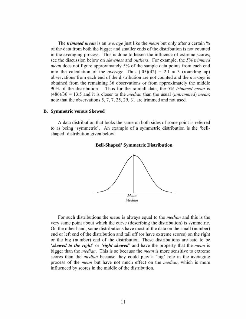
A data distribution that looks the same on both sides of some point is referred

to as being ‘symmetric’. An example of a symmetric distribution is the ‘bell-shaped’ distribution given below.

Bell-Shaped’ Symmetric Distribution

MeanMedian

For such distributions the mean is always equal to the median and this is the very same point about which the curve (describing the distribution) is symmetric. On the other hand, some distributions have most of the data on the small (number) end or left end of the distribution and tail off (or have extreme scores) on the right or the big (number) end of the distribution. These distributions are said to be ‘skewed to the right’ or ‘right skewed’ and have the property that the mean is bigger than the median. This is so because the mean is more sensitive to extreme scores than the median because they could play a ‘big’ role in the averaging process of the mean but have not much effect on the median, which is more influenced by scores in the middle of the distribution.

12

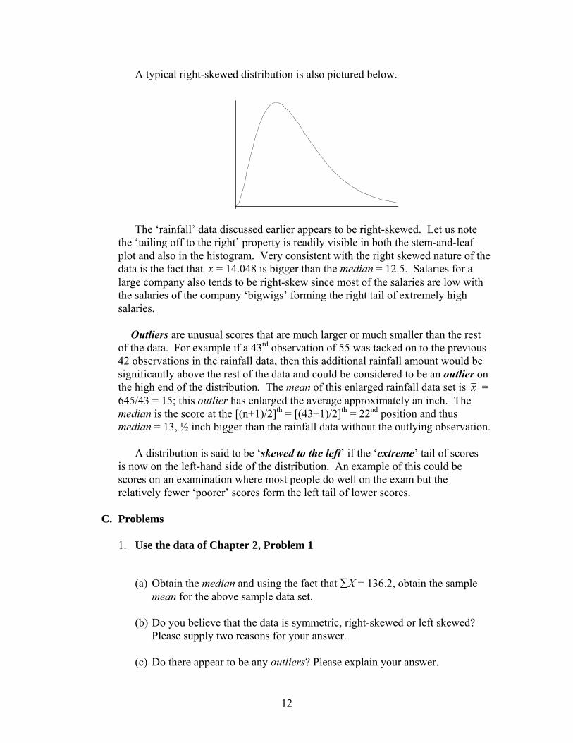
A typical right-skewed distribution is also pictured below.

The ‘rainfall’ data discussed earlier appears to be right-skewed. Let us note the ‘tailing off to the right’ property is readily visible in both the stem-and-leaf plot and also in the histogram. Very consistent with the right skewed nature of the data is the fact that x = 14.048 is bigger than the median = 12.5. Salaries for a large company also tends to be right-skew since most of the salaries are low with the salaries of the company ‘bigwigs’ forming the right tail of extremely high salaries.

Outliers are unusual scores that are much larger or much smaller than the rest

of the data. For example if a 43rd observation of 55 was tacked on to the previous 42 observations in the rainfall data, then this additional rainfall amount would be significantly above the rest of the data and could be considered to be an outlier on the high end of the distribution. The mean of this enlarged rainfall data set is x = 645/43 = 15; this outlier has enlarged the average approximately an inch. The median is the score at the [(n+1)/2]th = [(43+1)/2]th = 22nd position and thus median = 13, ½ inch bigger than the rainfall data without the outlying observation.

A distribution is said to be ‘skewed to the left’ if the ‘extreme’ tail of scores

is now on the left-hand side of the distribution. An example of this could be scores on an examination where most people do well on the exam but the relatively fewer ‘poorer’ scores form the left tail of lower scores.

C. Problems

1. Use the data of Chapter 2, Problem 1

(a) Obtain the median and using the fact that ∑X = 136.2, obtain the sample mean for the above sample data set.

(b) Do you believe that the data is symmetric, right-skewed or left skewed?

Please supply two reasons for your answer. (c) Do there appear to be any outliers? Please explain your answer.

13

2. Use the data of Chapter 2, Problem 2

(a) Obtain the median and using the fact that ∑X = 771, obtain the sample mean for the above sample data set.

(b) Do you believe that the data is symmetric, right-skewed or left skewed?

Please supply two reasons for your answer. 3. Use the data of Chapter 2, Problem 3

(a) Obtain the median and using the fact that ∑X = 149.3, obtain the sample mean for the above sample data set.

(b) Do there appear to be any outliers? Please explain your answer.

4. The number of million $ homes sold in 2000 for Bay Area communities are

206, 150, 173, 119, 228, 155, 348, 121, 124, 197, 275, 132 (a) Obtain the mean and the median. (b) Do you believe that the data is symmetric, right-skewed or left skewed?

Please supply two reasons for your answer.

14

IV. Measures of Variation (or Dispersion)

A. Range, Variance, Standard deviation

The 3 statistics (of course all based on the sample) the range, variance, and standard deviation, all measure the spread of the data. The range is simply given by the relationship, range = max – min. For the ‘rainfall’ data, range = (31-5) = 26; note that this statistic is extremely sensitive to even one unusually high or unusually low score.

The sample variance, denoted by s2, is given by the formula,

1)( 2

2

−

−= ∑

nxx

s ,

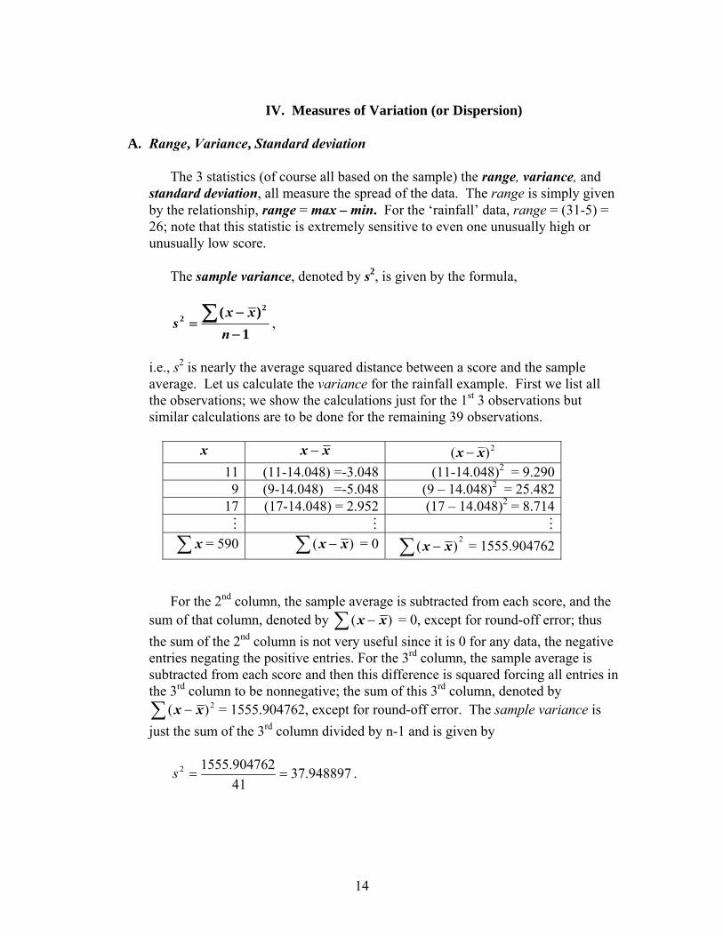
i.e., s2 is nearly the average squared distance between a score and the sample average. Let us calculate the variance for the rainfall example. First we list all the observations; we show the calculations just for the 1st 3 observations but similar calculations are to be done for the remaining 39 observations.

x xx − 2)( xx − 11 (11-14.048) =-3.048 (11-14.048)2 = 9.290 9 (9-14.048) =-5.048 (9 – 14.048)2 = 25.482

17 (17-14.048) = 2.952 (17 – 14.048)2 = 8.714

∑ x = 590 ∑ − )( xx = 0 2)(∑ − xx = 1555.904762

For the 2nd column, the sample average is subtracted from each score, and the sum of that column, denoted by ∑ − )( xx = 0, except for round-off error; thus the sum of the 2nd column is not very useful since it is 0 for any data, the negative entries negating the positive entries. For the 3rd column, the sample average is subtracted from each score and then this difference is squared forcing all entries in the 3rd column to be nonnegative; the sum of this 3rd column, denoted by ∑ − 2)( xx = 1555.904762, except for round-off error. The sample variance is just the sum of the 3rd column divided by n-1 and is given by

948897.3741904762.15552 ==s .

15

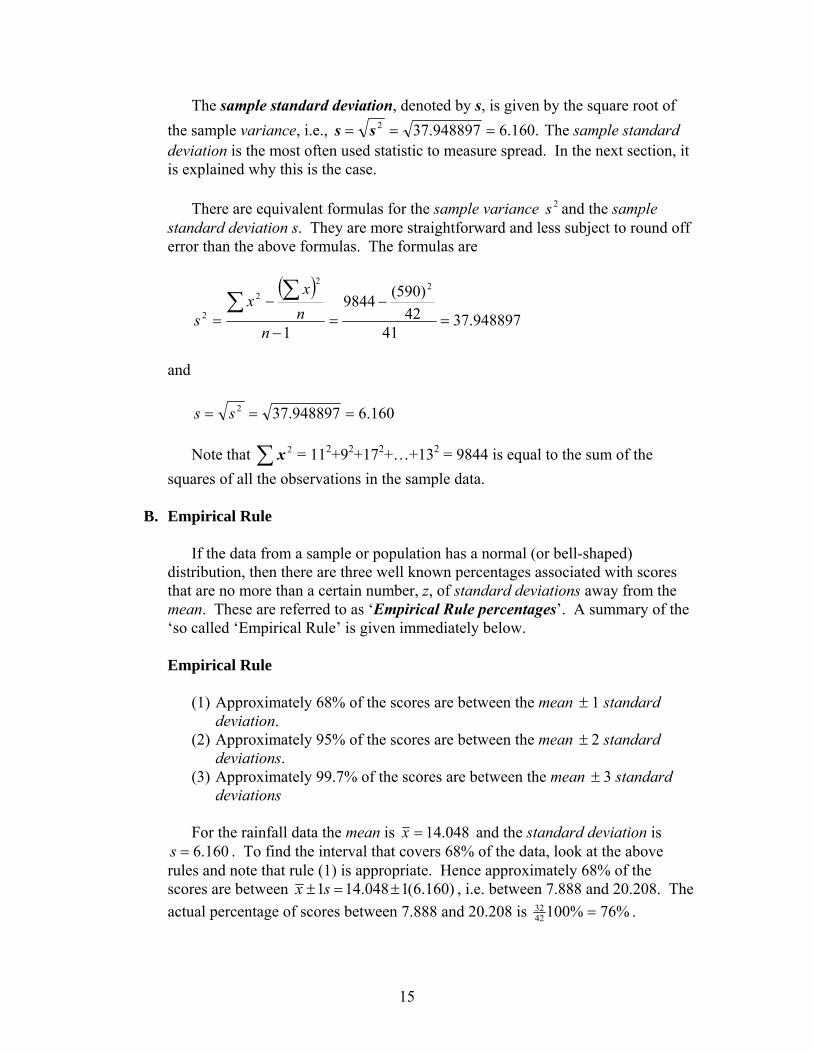
The sample standard deviation, denoted by s, is given by the square root of the sample variance, i.e., .160.6948897.372 === ss The sample standard deviation is the most often used statistic to measure spread. In the next section, it is explained why this is the case.

There are equivalent formulas for the sample variance 2s and the sample

standard deviation s. They are more straightforward and less subject to round off error than the above formulas. The formulas are

( )

1

2

2

2

−

−=

∑ ∑

nnx

xs 948897.37

4142

)590(98442

=−

=

and

160.6948897.372 === ss

Note that ∑ 2x = 112+92+172+…+132 = 9844 is equal to the sum of the squares of all the observations in the sample data.

B. Empirical Rule

If the data from a sample or population has a normal (or bell-shaped) distribution, then there are three well known percentages associated with scores that are no more than a certain number, z, of standard deviations away from the mean. These are referred to as ‘Empirical Rule percentages’. A summary of the ‘so called ‘Empirical Rule’ is given immediately below.

Empirical Rule

(1) Approximately 68% of the scores are between the mean ± 1 standard deviation.

(2) Approximately 95% of the scores are between the mean ± 2 standard deviations.

(3) Approximately 99.7% of the scores are between the mean ± 3 standard deviations

For the rainfall data the mean is 048.14=x and the standard deviation is

160.6=s . To find the interval that covers 68% of the data, look at the above rules and note that rule (1) is appropriate. Hence approximately 68% of the scores are between 1 14.048 1(6.160)x s± = ± , i.e. between 7.888 and 20.208. The actual percentage of scores between 7.888 and 20.208 is %76%10042

32 = .

16

Similarly: Approximately 95% of the scores are between 2 14.048 2(6.160)x s± = ± , i.e. between 1.728 and 26.368. The actual percentage

of scores between 1.728 and 26.368 is %95%1004240 = .

Approximately 99.7% of the scores are between 3 14.048 3(6.160)x s± = ± ,

i.e., between -4.432 and 32.528. The actual percentage of scores between -4.432 and 32.528 is %100%10042

42 = . The first of the above intervals contains all scores that are within one standard

deviation of the mean. For perfectly normal data, 68% all scores should fall in this first interval. For the rainfall example, we also obtain the ‘actual %’ of the 42 observations that fall within one standard deviation of the mean and this turns out to be 76%. There are occasions where based on a severe discrepancy between the empirical rule %’s (those based on normal theory) and the actual %’s, one would conclude that the sample data was not taken from a normal population. Also, especially for normal data, one could surmise how unusual an individual observed score is, by noting its number of standard deviations away from the mean. The greater the number of standard deviations, the more unusual the score.

C. Percentiles, Quartiles, Box-Plots

To get the 100pth percentile for the ‘rainfall data’ given above, one determines the rank (i.e. position) of the percentile, as was done earlier for the median; this is the score ranked approximately %100 p× of the scores up from the small end (i.e., left-hand end) of the distribution of scores.

For example, for p = .25, which designates the 100(.25) = 25th percentile, this

indicates a score that is approximately 25% up from the left-hand end of the distribution (or equivalently 75% (of the scores) down from the large (i.e. right-hand) end of the distribution). Suppose that the data set is a sample of login times (in minutes) on the Internet:

9.1 12.2 4.1 27.9 15.28.3 5.9 2.0 23.1 15.87.5 12.6 3.8 4.5 21.8

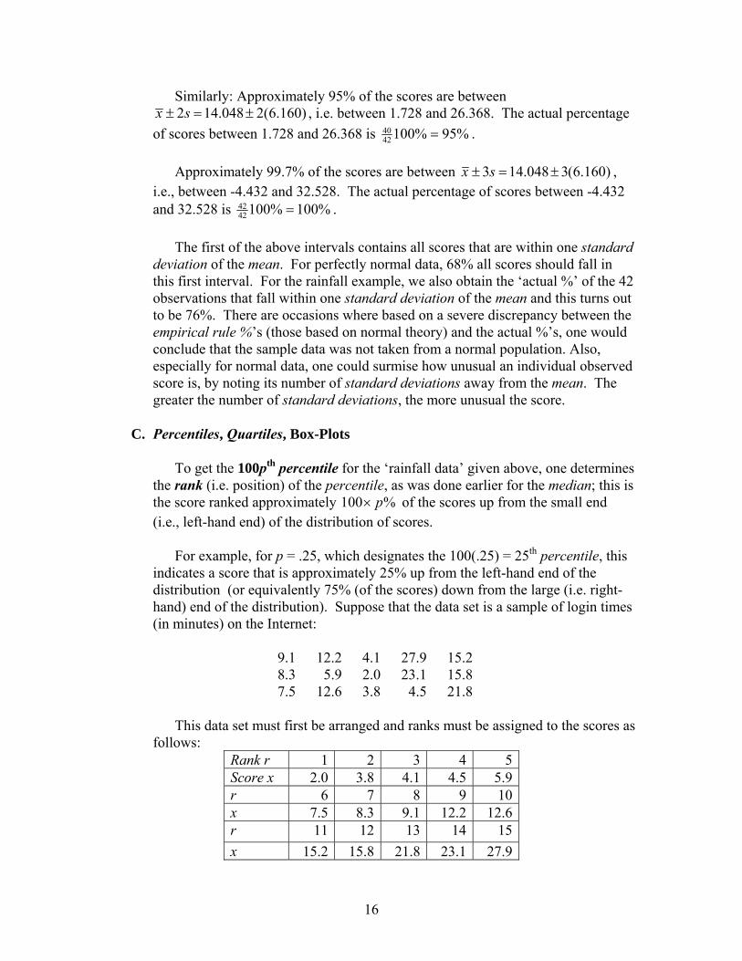
This data set must first be arranged and ranks must be assigned to the scores as

follows: Rank r 1 2 3 4 5Score x 2.0 3.8 4.1 4.5 5.9r 6 7 8 9 10x 7.5 8.3 9.1 12.2 12.6r 11 12 13 14 15x 15.2 15.8 21.8 23.1 27.9

17

To get the rank r of the 25th percentile, one multiplies the sample size plus 1 by p: 4)25(.16)1( ==×+= pnr .The 25th percentile 1Q is the score 4.5 whose rank is 4. Approximately 25% of the data is 4.5 or smaller.

The rank of the median, i.e. the 50th percentile is 8)50(.16)1( ==×+= pnr .

Hence, the median is the score 9.1 whose rank is 8. The rank of the 75th percentile 3Q is 12)75(.16)1( ==×+= pnr . Thus 3Q

is 15.8. Usually pnr ×+= )1( is not a whole number. For example the rank of the 40th percentile is 4.6)4(.16)1( ==×+= pnr

which is not a whole number. The 40th percentile is found by interpolation between the score 7.5 whose rank is 6 and the score 8.3 whose rank is 7 as follows: The 40th percentile = 7.5 (6.4 6)(8.3 7.5) 7.5 .4(.8) 7.5 .32 7.82+ − − = + = + = .

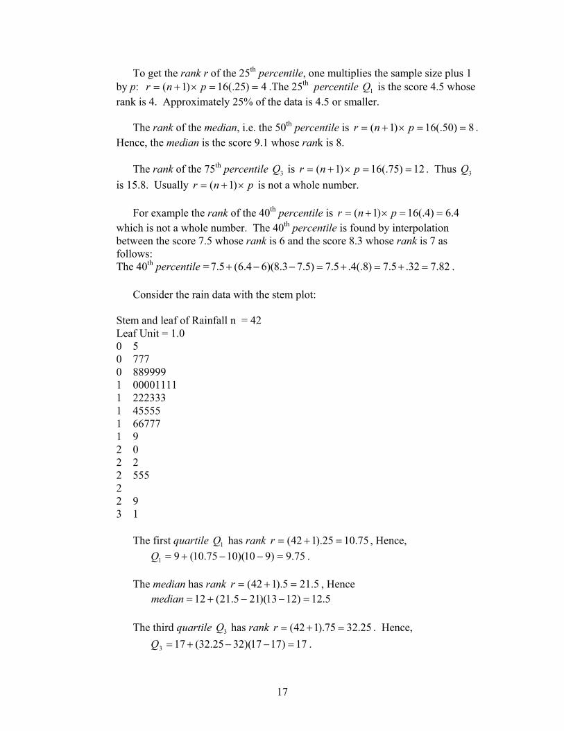
Consider the rain data with the stem plot:

Stem and leaf of Rainfall n = 42 Leaf Unit = 1.0 0 5 0 777 0 889999 1 00001111 1 222333 1 45555 1 66777 1 9 2 0 2 2 2 555 2 2 9 3 1

The first quartile 1Q has rank 75.1025).142( =+=r , Hence,

75.9)910)(1075.10(91 =−−+=Q .

The median has rank 5.215).142( =+=r , Hence 5.12)1213)(215.21(12 =−−+=median

The third quartile 3Q has rank 25.3275).142( =+=r . Hence,

17)1717)(3225.32(173 =−−+=Q .

18

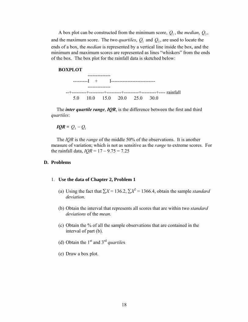
A box plot can be constructed from the minimum score, 1Q , the median, 3Q , and the maximum score. The two quartiles, 1Q and 3Q , are used to locate the ends of a box, the median is represented by a vertical line inside the box, and the minimum and maximum scores are represented as lines “whiskers” from the ends of the box. The box plot for the rainfall data is sketched below:

BOXPLOT -------------- ---------I + I--------------------------- -------------- --+---------+---------+---------+---------+---------+---- rainfall 5.0 10.0 15.0 20.0 25.0 30.0

The inter quartile range, IQR, is the difference between the first and third

quartiles: IQR = 13 QQ − The IQR is the range of the middle 50% of the observations. It is another

measure of variation; which is not as sensitive as the range to extreme scores. For the rainfall data, IQR = 17 – 9.75 = 7.25

D. Problems

1. Use the data of Chapter 2, Problem 1

(a) Using the fact that ∑X = 136.2, ∑X2 = 1366.4, obtain the sample standard deviation.

(b) Obtain the interval that represents all scores that are within two standard

deviations of the mean. (c) Obtain the % of all the sample observations that are contained in the

interval of part (b). (d) Obtain the 1st and 3rd quartiles (e) Draw a box plot.

19

2. Use the data of Chapter 2, Problem 2

(a) Using the fact that ∑X = 771, ∑X2 = 27323, obtain the sample standard deviation.

(b) Obtain the interval that represents all scores that are within one standard

deviation of the mean. (c) Obtain the % of all the sample observations that are contained in the

interval of part (b). (d) Obtain the 1st and 3rd quartiles. (e) Draw a box plot.

(f) Do you believe that the sample data follows a bell curve, i.e., is normal?

Supply 2 reasons for your answer.

20

3. Use the data of Chapter 2, Problem 3

(a) Using the fact that ∑X = 149.3, ∑X2 = 1484.5, obtain the sample standard deviation.

(b) Obtain the interval that represents all scores that are within three standard

deviations of the mean. (c) Obtain the % of all the sample observations that are contained in the

interval of part (b). (d) Obtain the 1st and 3rd quartiles. (e) Draw a box plot.

4. Use the ‘homes’ data of Chapter 3, Problem 4 (a) Obtain ∑X and ∑X2 . (b) Obtain the sample standard deviation. (c) Obtain the 1st and 3rd quartiles (d) Draw a boxplot.

21

Problems on the Empirical Rule

5. Suppose that Fred uses an average of 21.7 gallons of gas per week with a standard deviation 5.2 gallons. Fred has found that his weekly gas usage has a mound shaped distribution.

(a) What % of the time is his weekly usage between 11.3 and 32.1 gallons? (b) What % of the time is his weekly usage between 16.5 and 26.9 gallons? (c) 99.7% of the time his weekly gas usage is between what two amounts?

This is a more difficult and challenging Problem 6. The time that it takes a certain professor to get to work is normally distributed

with a mean of 70 minutes and a standard deviation of 8 minutes. (a) What % of time does it take her at most 54 minutes to get to work? (b) What % of time does it take her at least 78 minutes to get to work?

(c) What % of time does it take her between 70 and 94 minutes to get to work?

22

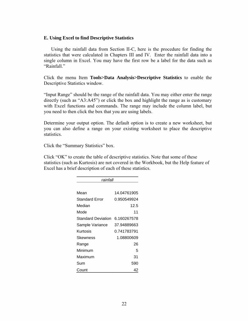
E. Using Excel to find Descriptive Statistics

Using the rainfall data from Section II-C, here is the procedure for finding the

statistics that were calculated in Chapters III and IV. Enter the rainfall data into a single column in Excel. You may have the first row be a label for the data such as “Rainfall.”

Click the menu Item Tools>Data Analysis>Descriptive Statistics to enable the

Descriptive Statistics window.

“Input Range” should be the range of the rainfall data. You may either enter the range directly (such as “A3:A45”) or click the box and highlight the range as is customary with Excel functions and commands. The range may include the column label, but you need to then click the box that you are using labels.

Determine your output option. The default option is to create a new worksheet, but

you can also define a range on your existing worksheet to place the descriptive statistics.

Click the “Summary Statistics” box.

Click “OK” to create the table of descriptive statistics. Note that some of these statistics (such as Kurtosis) are not covered in the Workbook, but the Help feature of Excel has a brief description of each of these statistics.

rainfall

Mean 14.04761905Standard Error 0.950549924Median 12.5Mode 11Standard Deviation 6.160267578Sample Variance 37.94889663Kurtosis 0.741783791Skewness 1.08800609Range 26Minimum 5Maximum 31Sum 590Count 42

23

V. Probability

A. Empirical Definition versus Classical (or Counting) Definition

Empirical Definition Probability = long-run relative frequency

For example, P(H = head) = probability of achieving a head by throwing a coin, is normally thought to be equal to 0.5; a coin with 50% chance of falling heads is referred to as a fair coin. This value could have been gotten by throwing a coin 10,000 (long-run) times and noting that the relative frequency of heads was (4970 heads)/10,000 or approximately 0.5. If we would have gotten a relative frequency of (5970 heads)/10000 ≈ .60, we would be inclined to say that the coin was not fair but was biased towards heads.

For a 2nd example, if one was interested in the proportion of people in a

certain population that favored at least the partial privatization of Social Security, referred to as P(randomly choosing someone from the population that favors privatization), one could randomly sample 1000 (long-run) individuals from the population and observe the number favoring privatization, say 583 and then the relative frequency favoring privatization is (583/1000) = .583 and it could be concluded that P(privatization) ≈ .583.

Counting Definition

An event is a collection of outcomes of an experiment.

experiment the of outcomes ofnumber total Theevent the to favorable outcomes ofNumber (event) =P

This definition assumes that all the possible outcomes of the experiment are equally likely.

For example, since for a fair coin there are two equally likely outcomes, H(eads) and T(ails), P(H) = ½. Also, for a throw of a fair die since there are six equally likely outcomes, namely 1-6, P(1) = 1/6; also P(odd no. showing) = 3/6 since the number of outcomes favorable to the event odd no. showing is 3, namely {1,3,5}.

For another example, we will show later on that the number of possible 5 card

poker hands (randomly chosen from 52 cards) is 2,598,960. The probability of a royal flush is (4)/2,598,960 = 1/649,740, since there a 4 possible hands giving a royal flush, namely 10 through ace, of one of 4 possible suits: clubs, spades, diamonds or hearts.

24

For a 3rd example, suppose a population consists of 1,000,000 people, 600,000

of them favoring privatization of Social Security and 400,000 of them against privatization. Suppose one individual is randomly selected from the population, the P(individual selected favors privatization) = (600,000)/1,000,000 = .60 and in this context probability can be regarded as a population proportion.

B Combinations

‘Lot’ Example Using Counting

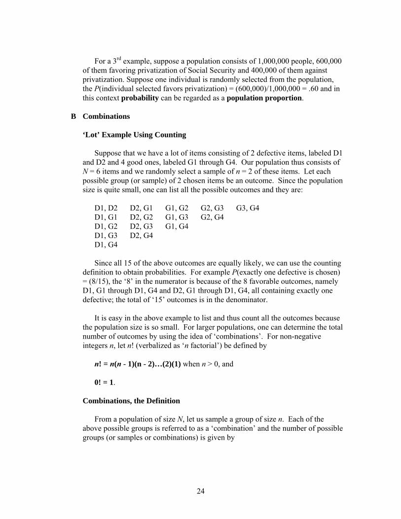
Suppose that we have a lot of items consisting of 2 defective items, labeled D1 and D2 and 4 good ones, labeled G1 through G4. Our population thus consists of N = 6 items and we randomly select a sample of n = 2 of these items. Let each possible group (or sample) of 2 chosen items be an outcome. Since the population size is quite small, one can list all the possible outcomes and they are:

D1, D2 D2, G1 G1, G2 G2, G3 G3, G4 D1, G1 D2, G2 G1, G3 G2, G4 D1, G2 D2, G3 G1, G4 D1, G3 D2, G4 D1, G4 Since all 15 of the above outcomes are equally likely, we can use the counting

definition to obtain probabilities. For example P(exactly one defective is chosen) = (8/15), the ‘8’ in the numerator is because of the 8 favorable outcomes, namely D1, G1 through D1, G4 and D2, G1 through D1, G4, all containing exactly one defective; the total of ‘15’ outcomes is in the denominator.

It is easy in the above example to list and thus count all the outcomes because

the population size is so small. For larger populations, one can determine the total number of outcomes by using the idea of ‘combinations’. For non-negative integers n, let n! (verbalized as ‘n factorial’) be defined by

n! = n(n - 1)(n - 2)…(2)(1) when n > 0, and 0! = 1.

Combinations, the Definition

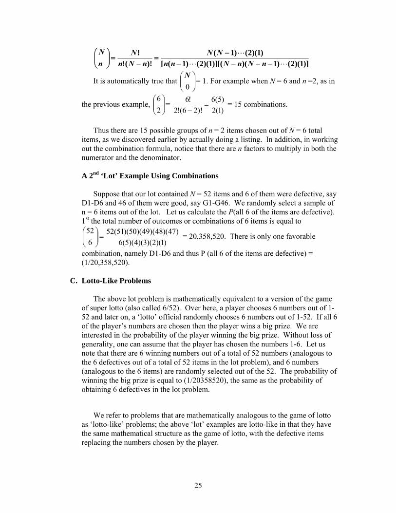
From a population of size N, let us sample a group of size n. Each of the above possible groups is referred to as a ‘combination’ and the number of possible groups (or samples or combinations) is given by

25

)]1)(2()1)()][(1)(2()1([

)1)(2()1()!(!

!−−−−

−=

−=⎟⎟

⎠

⎞⎜⎜⎝

⎛nNnNnn

NNnNn

NnN

It is automatically true that ⎟⎟⎠

⎞⎜⎜⎝

⎛0N

= 1. For example when N = 6 and n =2, as in

the previous example, ⎟⎟⎠

⎞⎜⎜⎝

⎛26

= )1(2)5(6

)!26(!2!6

=−

= 15 combinations.

Thus there are 15 possible groups of n = 2 items chosen out of N = 6 total

items, as we discovered earlier by actually doing a listing. In addition, in working out the combination formula, notice that there are n factors to multiply in both the numerator and the denominator.

A 2nd ‘Lot’ Example Using Combinations

Suppose that our lot contained N = 52 items and 6 of them were defective, say D1-D6 and 46 of them were good, say G1-G46. We randomly select a sample of n = 6 items out of the lot. Let us calculate the P(all 6 of the items are defective). 1st the total number of outcomes or combinations of 6 items is equal to

)1)(2)(3)(4)(5(6)47)(48)(49)(50)(51(52

652

=⎟⎟⎠

⎞⎜⎜⎝

⎛ = 20,358,520. There is only one favorable

combination, namely D1-D6 and thus P (all 6 of the items are defective) = (1/20,358,520).

C. Lotto-Like Problems

The above lot problem is mathematically equivalent to a version of the game of super lotto (also called 6/52). Over here, a player chooses 6 numbers out of 1-52 and later on, a ‘lotto’ official randomly chooses 6 numbers out of 1-52. If all 6 of the player’s numbers are chosen then the player wins a big prize. We are interested in the probability of the player winning the big prize. Without loss of generality, one can assume that the player has chosen the numbers 1-6. Let us note that there are 6 winning numbers out of a total of 52 numbers (analogous to the 6 defectives out of a total of 52 items in the lot problem), and 6 numbers (analogous to the 6 items) are randomly selected out of the 52. The probability of winning the big prize is equal to (1/20358520), the same as the probability of obtaining 6 defectives in the lot problem.

We refer to problems that are mathematically analogous to the game of lotto as ‘lotto-like’ problems; the above ‘lot’ examples are lotto-like in that they have the same mathematical structure as the game of lotto, with the defective items replacing the numbers chosen by the player.

26

In super lotto, as described above, a lesser prize is won if only five of the player’s numbers, say 1-5 and 36, are randomly selected by the official, and the player’s numbers are 1-6. A more difficult problem is to obtain the P (exactly 5 of the players numbers are selected).

We proceed to evaluate this probability. The total number of outcomes is

unchanged and is equal to ⎟⎟⎠

⎞⎜⎜⎝

⎛6

52 = 20358520. The number of favorable outcomes

is given by (the number of 5 number combinations chosen from 1-6, these are the possible 5 selected player numbers) x (the number of 1 number combinations

chosen from 7-52, these are the possible one selected non-player number) = ⎟⎟⎠

⎞⎜⎜⎝

⎛56 x

⎟⎟⎠

⎞⎜⎜⎝

⎛146 = 6(46); the 6, 5-numbered combinations include {1-5; 1-4, 6; 1-3, 5-6; 1-2,

4-6; 1, 3-6; 2-6} and the 46, 1-numbered combinations include {7; 8; … ;52}. The probability of exactly 5 selected players numbers is thus [6(46)]/20358520.

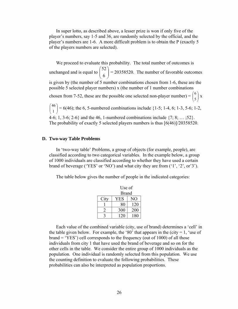
D. Two-way Table Problems

In ‘two-way table’ Problems, a group of objects (for example, people), are classified according to two categorical variables. In the example below, a group of 1000 individuals are classified according to whether they have used a certain brand of beverage (‘YES’ or ‘NO’) and what city they are from (‘1’, ‘2’, or’3’).

The table below gives the number of people in the indicated categories:

Use of Brand

City YES NO 1 80 1202 300 2003 120 180

Each value of the combined variable (city, use of brand) determines a ‘cell’ in

the table given below. For example, the ‘80’ that appears in the (city = 1, ‘use of brand = ‘YES’) cell corresponds to the frequency (out of 1000) of all those individuals from city 1 that have used the brand of beverage and so on for the other cells in the table. We consider the entire group of 1000 individuals as the population. One individual is randomly selected from this population. We use the counting definition to evaluate the following probabilities. These probabilities can also be interpreted as population proportions.

27

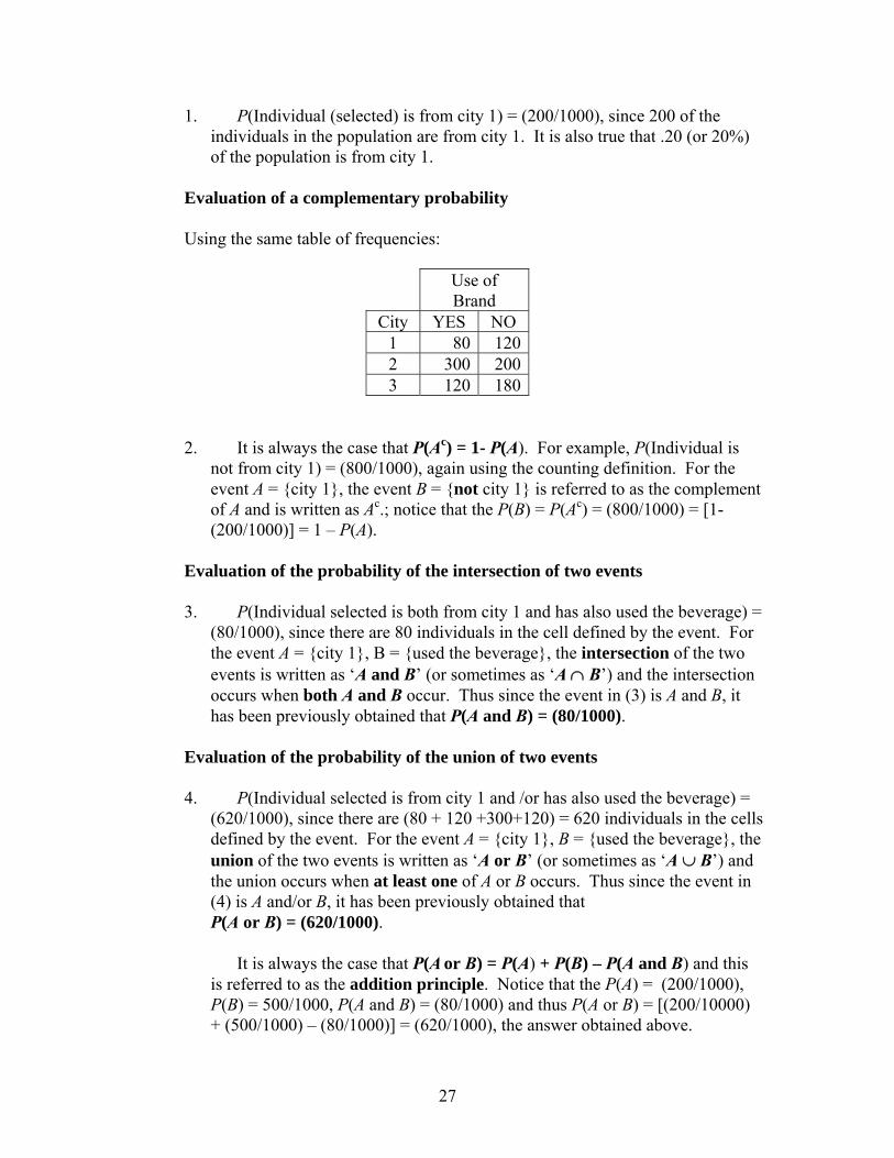
1. P(Individual (selected) is from city 1) = (200/1000), since 200 of the individuals in the population are from city 1. It is also true that .20 (or 20%) of the population is from city 1.

Evaluation of a complementary probability Using the same table of frequencies:

Use of Brand

City YES NO 1 80 1202 300 2003 120 180

2. It is always the case that P(Ac) = 1- P(A). For example, P(Individual is

not from city 1) = (800/1000), again using the counting definition. For the event A = {city 1}, the event B = {not city 1} is referred to as the complement of A and is written as Ac.; notice that the P(B) = P(Ac) = (800/1000) = [1-(200/1000)] = 1 – P(A).

Evaluation of the probability of the intersection of two events 3. P(Individual selected is both from city 1 and has also used the beverage) =

(80/1000), since there are 80 individuals in the cell defined by the event. For the event A = {city 1}, B = {used the beverage}, the intersection of the two events is written as ‘A and B’ (or sometimes as ‘A ∩ B’) and the intersection occurs when both A and B occur. Thus since the event in (3) is A and B, it has been previously obtained that P(A and B) = (80/1000).

Evaluation of the probability of the union of two events 4. P(Individual selected is from city 1 and /or has also used the beverage) =

(620/1000), since there are (80 + 120 +300+120) = 620 individuals in the cells defined by the event. For the event A = {city 1}, B = {used the beverage}, the union of the two events is written as ‘A or B’ (or sometimes as ‘A ∪ B’) and the union occurs when at least one of A or B occurs. Thus since the event in (4) is A and/or B, it has been previously obtained that P(A or B) = (620/1000).

It is always the case that P(A or B) = P(A) + P(B) – P(A and B) and this is referred to as the addition principle. Notice that the P(A) = (200/1000), P(B) = 500/1000, P(A and B) = (80/1000) and thus P(A or B) = [(200/10000) + (500/1000) – (80/1000)] = (620/1000), the answer obtained above.

28

Conditional Probability Again using the same table of frequencies:

Use of Brand

City YES NO 1 80 1202 300 2003 120 180

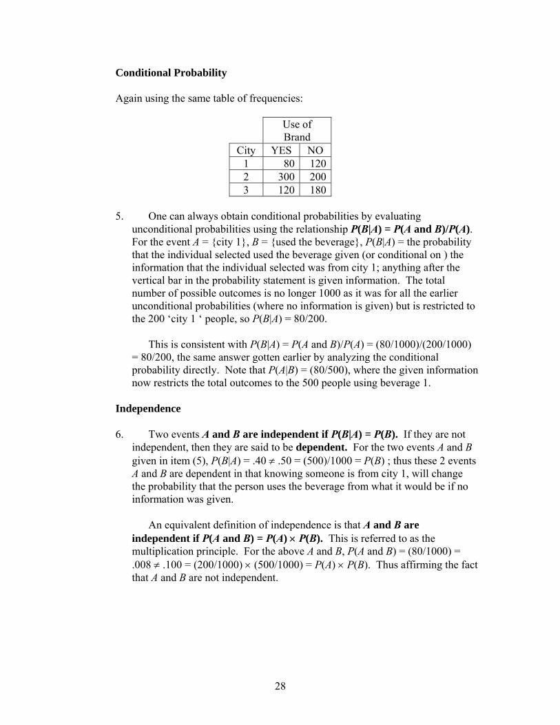
5. One can always obtain conditional probabilities by evaluating

unconditional probabilities using the relationship P(B|A) = P(A and B)/P(A). For the event A = {city 1}, B = {used the beverage}, P(B|A) = the probability that the individual selected used the beverage given (or conditional on ) the information that the individual selected was from city 1; anything after the vertical bar in the probability statement is given information. The total number of possible outcomes is no longer 1000 as it was for all the earlier unconditional probabilities (where no information is given) but is restricted to the 200 ‘city 1 ‘ people, so P(B|A) = 80/200.

This is consistent with P(B|A) = P(A and B)/P(A) = (80/1000)/(200/1000)

= 80/200, the same answer gotten earlier by analyzing the conditional probability directly. Note that P(A|B) = (80/500), where the given information now restricts the total outcomes to the 500 people using beverage 1.

Independence 6. Two events A and B are independent if P(B|A) = P(B). If they are not

independent, then they are said to be dependent. For the two events A and B given in item (5), P(B|A) = .40 ≠ .50 = (500)/1000 = P(B) ; thus these 2 events A and B are dependent in that knowing someone is from city 1, will change the probability that the person uses the beverage from what it would be if no information was given.

An equivalent definition of independence is that A and B are

independent if P(A and B) = P(A) × P(B). This is referred to as the multiplication principle. For the above A and B, P(A and B) = (80/1000) = .008 ≠ .100 = (200/1000) × (500/1000) = P(A) × P(B). Thus affirming the fact that A and B are not independent.

29

E. Qualitative versus Quantitative Variables & Discrete versus Continuous Variables

If the measurements of a variable are numerical, then the variable is called quantitative.

If the possible values of a quantitative variable can be counted, then the variable is called discrete.

If a quantitative variable can have any numerical value in an interval, then the variable is called continuous. If the values of a variable are categories, then the variable is called qualitative.

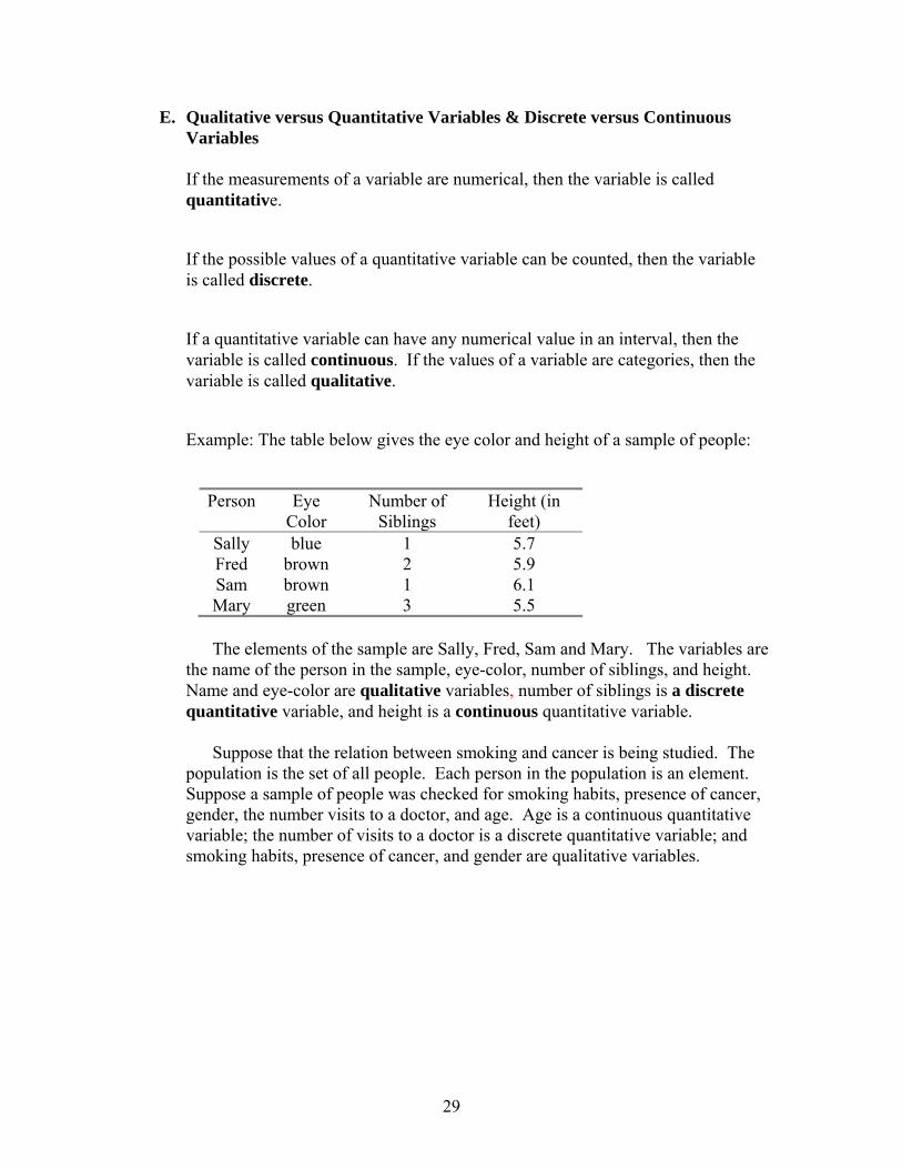
Example: The table below gives the eye color and height of a sample of people:

Person Eye Color

Number of Siblings

Height (in feet)

Sally blue 1 5.7 Fred brown 2 5.9 Sam brown 1 6.1 Mary green 3 5.5

The elements of the sample are Sally, Fred, Sam and Mary. The variables are

the name of the person in the sample, eye-color, number of siblings, and height. Name and eye-color are qualitative variables, number of siblings is a discrete quantitative variable, and height is a continuous quantitative variable.

Suppose that the relation between smoking and cancer is being studied. The

population is the set of all people. Each person in the population is an element. Suppose a sample of people was checked for smoking habits, presence of cancer, gender, the number visits to a doctor, and age. Age is a continuous quantitative variable; the number of visits to a doctor is a discrete quantitative variable; and smoking habits, presence of cancer, and gender are qualitative variables.

30

F. Problems

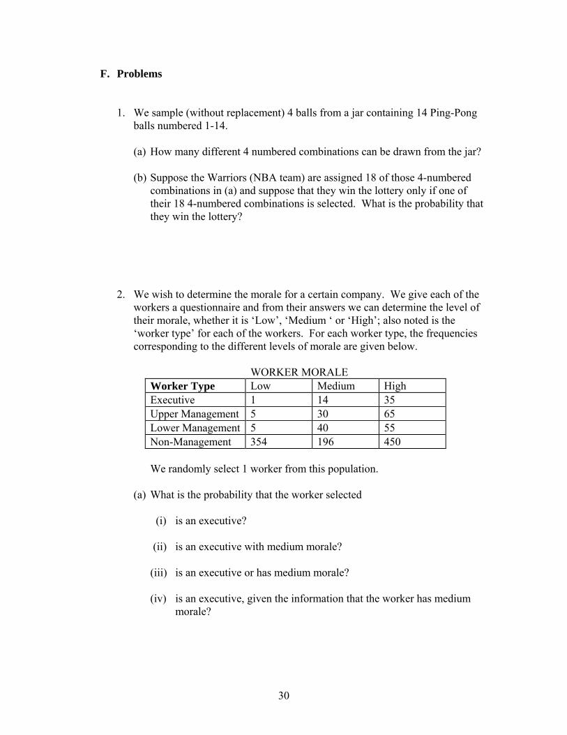
1. We sample (without replacement) 4 balls from a jar containing 14 Ping-Pong balls numbered 1-14.

(a) How many different 4 numbered combinations can be drawn from the jar? (b) Suppose the Warriors (NBA team) are assigned 18 of those 4-numbered

combinations in (a) and suppose that they win the lottery only if one of their 18 4-numbered combinations is selected. What is the probability that they win the lottery?

2. We wish to determine the morale for a certain company. We give each of the

workers a questionnaire and from their answers we can determine the level of their morale, whether it is ‘Low’, ‘Medium ‘ or ‘High’; also noted is the ‘worker type’ for each of the workers. For each worker type, the frequencies corresponding to the different levels of morale are given below.

WORKER MORALE

Worker Type Low Medium High Executive 1 14 35 Upper Management 5 30 65 Lower Management 5 40 55 Non-Management 354 196 450

We randomly select 1 worker from this population.

(a) What is the probability that the worker selected

(i) is an executive? (ii) is an executive with medium morale? (iii) is an executive or has medium morale? (iv) is an executive, given the information that the worker has medium

morale?

31

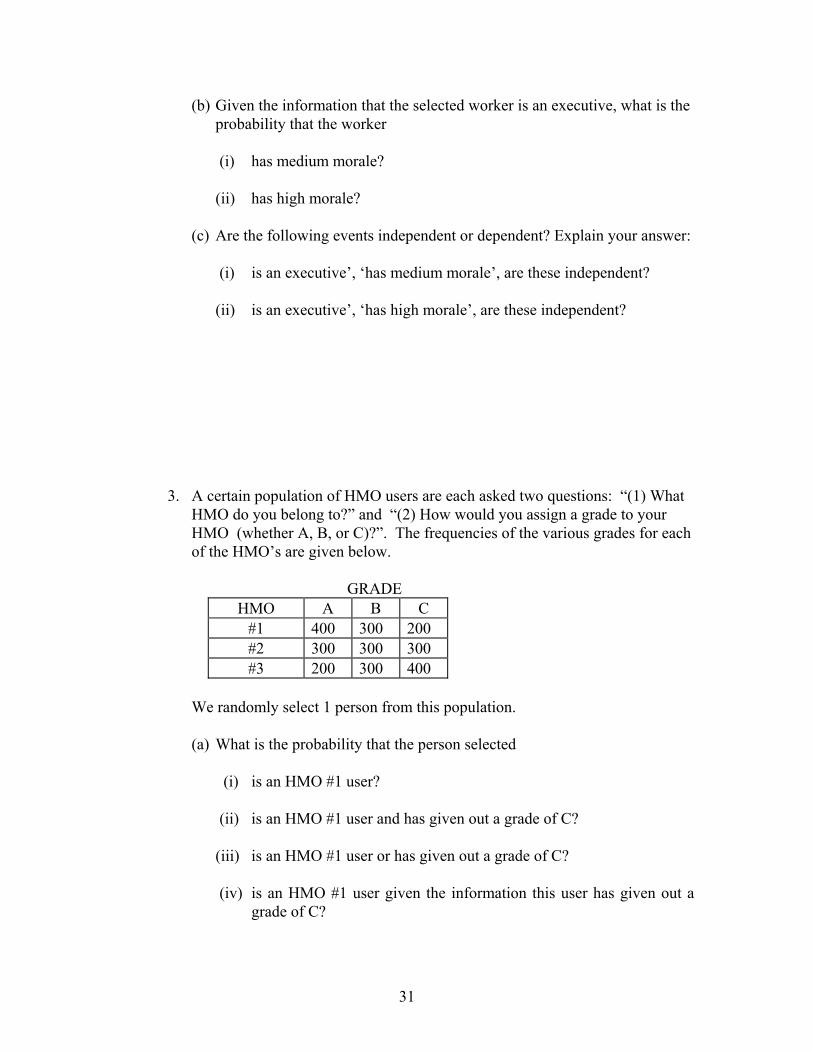
(b) Given the information that the selected worker is an executive, what is the probability that the worker

(i) has medium morale? (ii) has high morale?

(c) Are the following events independent or dependent? Explain your answer:

(i) is an executive’, ‘has medium morale’, are these independent? (ii) is an executive’, ‘has high morale’, are these independent?

3. A certain population of HMO users are each asked two questions: “(1) What HMO do you belong to?” and “(2) How would you assign a grade to your HMO (whether A, B, or C)?”. The frequencies of the various grades for each of the HMO’s are given below.

GRADE

HMO A B C #1 400 300 200 #2 300 300 300 #3 200 300 400

We randomly select 1 person from this population. (a) What is the probability that the person selected

(i) is an HMO #1 user? (ii) is an HMO #1 user and has given out a grade of C? (iii) is an HMO #1 user or has given out a grade of C? (iv) is an HMO #1 user given the information this user has given out a

grade of C?

32

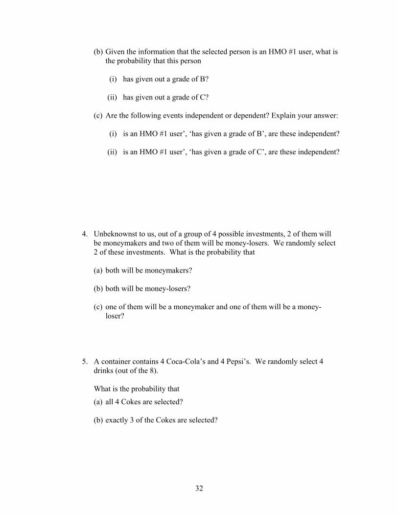
(b) Given the information that the selected person is an HMO #1 user, what is the probability that this person

(i) has given out a grade of B? (ii) has given out a grade of C?

(c) Are the following events independent or dependent? Explain your answer:

(i) is an HMO #1 user’, ‘has given a grade of B’, are these independent? (ii) is an HMO #1 user’, ‘has given a grade of C’, are these independent?

4. Unbeknownst to us, out of a group of 4 possible investments, 2 of them will be moneymakers and two of them will be money-losers. We randomly select 2 of these investments. What is the probability that

(a) both will be moneymakers? (b) both will be money-losers? (c) one of them will be a moneymaker and one of them will be a money-

loser?

5. A container contains 4 Coca-Cola’s and 4 Pepsi’s. We randomly select 4 drinks (out of the 8).

What is the probability that

(a) all 4 Cokes are selected? (b) exactly 3 of the Cokes are selected?

33

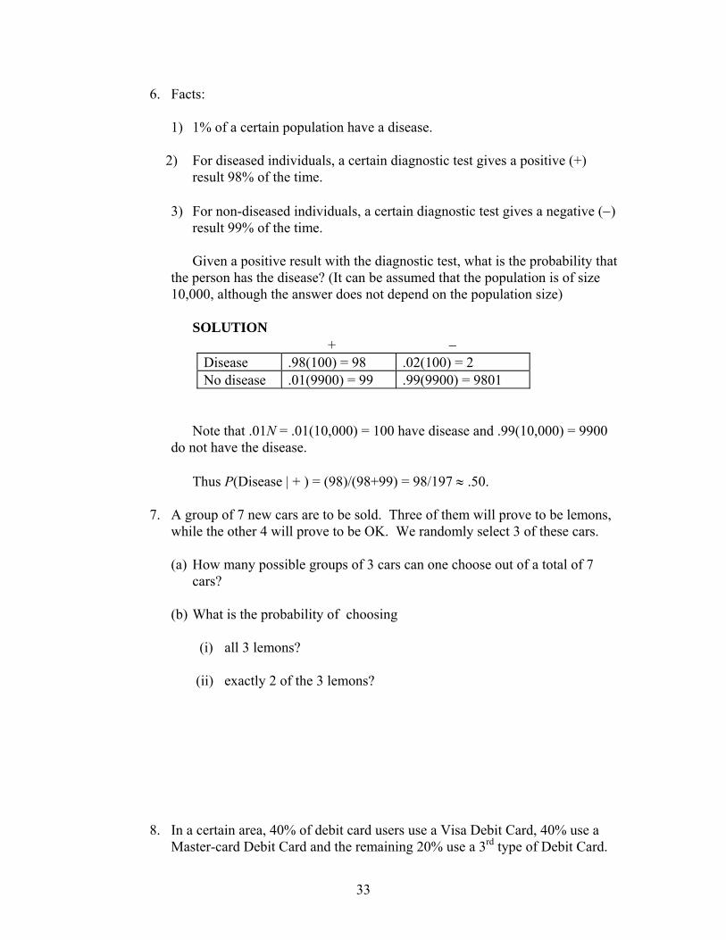
6. Facts: 1) 1% of a certain population have a disease.

2) For diseased individuals, a certain diagnostic test gives a positive (+) result 98% of the time.

3) For non-diseased individuals, a certain diagnostic test gives a negative (−)

result 99% of the time.

Given a positive result with the diagnostic test, what is the probability that the person has the disease? (It can be assumed that the population is of size 10,000, although the answer does not depend on the population size)

SOLUTION

+ − Disease .98(100) = 98 .02(100) = 2 No disease .01(9900) = 99 .99(9900) = 9801

Note that .01N = .01(10,000) = 100 have disease and .99(10,000) = 9900 do not have the disease.

Thus P(Disease | + ) = (98)/(98+99) = 98/197 ≈ .50.

7. A group of 7 new cars are to be sold. Three of them will prove to be lemons, while the other 4 will prove to be OK. We randomly select 3 of these cars.

(a) How many possible groups of 3 cars can one choose out of a total of 7

cars? (b) What is the probability of choosing

(i) all 3 lemons? (ii) exactly 2 of the 3 lemons?

8. In a certain area, 40% of debit card users use a Visa Debit Card, 40% use a Master-card Debit Card and the remaining 20% use a 3rd type of Debit Card.

34

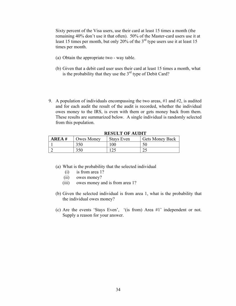
Sixty percent of the Visa users, use their card at least 15 times a month (the remaining 40% don’t use it that often). 50% of the Master-card users use it at least 15 times per month, but only 20% of the 3rd type users use it at least 15 times per month.

(a) Obtain the appropriate two - way table. (b) Given that a debit card user uses their card at least 15 times a month, what

is the probability that they use the 3rd type of Debit Card?

9. A population of individuals encompassing the two areas, #1 and #2, is audited and for each audit the result of the audit is recorded, whether the individual owes money to the IRS, is even with them or gets money back from them. These results are summarized below. A single individual is randomly selected from this population.

RESULT OF AUDIT

AREA # Owes Money Stays Even Gets Money Back 1 350 100 50 2 350 125 25

(a) What is the probability that the selected individual (i) is from area 1? (ii) owes money? (iii) owes money and is from area 1?

(b) Given the selected individual is from area 1, what is the probability that

the individual owes money? (c) Are the events ‘Stays Even’, ‘(is from) Area #1’ independent or not.

Supply a reason for your answer.

35

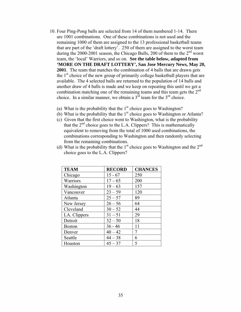
10. Four Ping-Pong balls are selected from 14 of them numbered 1-14. There are 1001 combinations. One of these combinations is not used and the remaining 1000 of them are assigned to the 13 professional basketball teams that are part of the ‘draft lottery’. 250 of them are assigned to the worst team during the 2000-2001 season, the Chicago Bulls, 200 of them to the 2nd worst team, the ‘local’ Warriors, and so on. See the table below, adapted from ‘MORE ON THE DRAFT LOTTERY’, San Jose Mercury News, May 20, 2001. The team that matches the combination of 4 balls that are drawn gets the 1st choice of the new group of primarily college basketball players that are available. The 4 selected balls are returned to the population of 14 balls and another draw of 4 balls is made and we keep on repeating this until we get a combination matching one of the remaining teams and this team gets the 2nd choice. In a similar manner, we obtain a 3rd team for the 3rd choice.

(a) What is the probability that the 1st choice goes to Washington? (b) What is the probability that the 1st choice goes to Washington or Atlanta? (c) Given that the first choice went to Washington, what is the probability

that the 2nd choice goes to the L.A. Clippers? This is mathematically equivalent to removing from the total of 1000 used combinations, the combinations corresponding to Washington and then randomly selecting from the remaining combinations.

(d) What is the probability that the 1st choice goes to Washington and the 2nd choice goes to the L.A. Clippers?

TEAM RECORD CHANCES Chicago 15 - 67 250 Warriors 17 – 65 200 Washington 19 – 63 157 Vancouver 23 – 59 120 Atlanta 25 – 57 89 New Jersey 26 – 56 64 Cleveland 30 – 52 44 LA. Clippers 31 – 51 29 Detroit 32 – 50 18 Boston 36 - 46 11 Denver 40 – 42 7 Seattle 44 – 38 6 Houston 45 – 37 5

36

11. The latest (as of June 2001) version of ‘Superlotto’ in Ca. is

‘SUPPERLOTTO PLUS’ as is given below, adapted from ‘POWERING UP SUPER LOTTO’ appearing in the San Francisco Chronicle (April 19, 2000); the former version also appears below as ‘SUPERLOTTO’. With reference to SUPPERLOTTO PLUS, What is the probability of

(a) winning the jackpot? (b) matching exactly 4 regular numbers and the Mega Number? (c) matching at least 4 regular numbers and the Mega Number?

SUPERLOTTO SUPERLOTTO PLUS How to play Players pick 6 numbers between 1 and 51. Players pick 5 numbers between 1 and 47

and a 6th number (‘Mega Number’) between 1 and 27.

How to win 1. Jackpot: Match all six numbers 2. Match 5 numbers 3. Match 4 numbers 4. Match 3 numbers

1. Jackpot: Match all 5 regular numbers and the Mega Number

2. Match five (regular)numbers without the mega number

3. Match 4 numbers and Mega Number 4. Match 1-3 No.’s and Mega Number 5. Match Mega Number only 6. Match 2-4 No.’s without Mega

Number How much you win

1. Millions 2. About $1500 3. $79 4. About $5

1. More likely to have over 100 million 2. Probably between 10K and 25K 3. Between $1200 and $1600 4. Between $10 and $100 5. $1

Odds of winning

Jackpot: 1 in 18 million At Least Something: 1 in 60

Jackpot: 1 in 41 million At Least Something: 1 in 23

37

VI. Discrete Probability Distributions

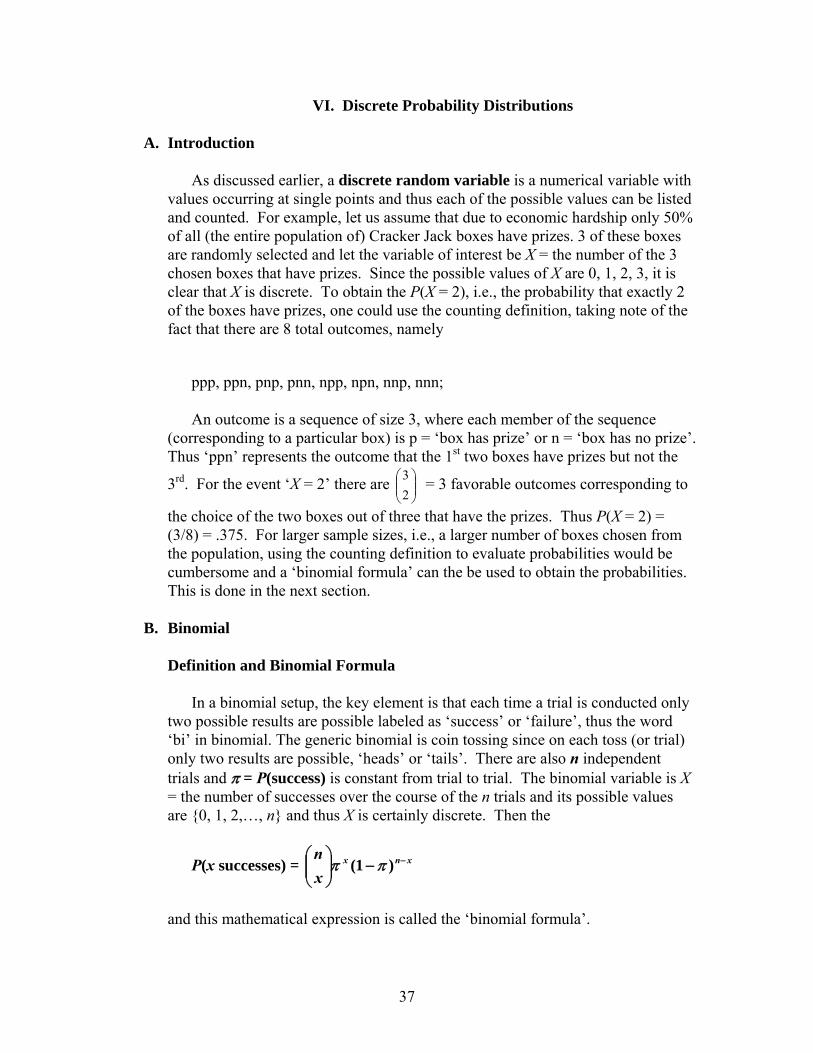
A. Introduction

As discussed earlier, a discrete random variable is a numerical variable with values occurring at single points and thus each of the possible values can be listed and counted. For example, let us assume that due to economic hardship only 50% of all (the entire population of) Cracker Jack boxes have prizes. 3 of these boxes are randomly selected and let the variable of interest be X = the number of the 3 chosen boxes that have prizes. Since the possible values of X are 0, 1, 2, 3, it is clear that X is discrete. To obtain the P(X = 2), i.e., the probability that exactly 2 of the boxes have prizes, one could use the counting definition, taking note of the fact that there are 8 total outcomes, namely

ppp, ppn, pnp, pnn, npp, npn, nnp, nnn; An outcome is a sequence of size 3, where each member of the sequence

(corresponding to a particular box) is p = ‘box has prize’ or n = ‘box has no prize’. Thus ‘ppn’ represents the outcome that the 1st two boxes have prizes but not the

3rd. For the event ‘X = 2’ there are ⎟⎟⎠

⎞⎜⎜⎝

⎛23 = 3 favorable outcomes corresponding to

the choice of the two boxes out of three that have the prizes. Thus P(X = 2) = (3/8) = .375. For larger sample sizes, i.e., a larger number of boxes chosen from the population, using the counting definition to evaluate probabilities would be cumbersome and a ‘binomial formula’ can the be used to obtain the probabilities. This is done in the next section.

B. Binomial

Definition and Binomial Formula

In a binomial setup, the key element is that each time a trial is conducted only two possible results are possible labeled as ‘success’ or ‘failure’, thus the word ‘bi’ in binomial. The generic binomial is coin tossing since on each toss (or trial) only two results are possible, ‘heads’ or ‘tails’. There are also n independent trials and π = P(success) is constant from trial to trial. The binomial variable is X = the number of successes over the course of the n trials and its possible values are {0, 1, 2,…, n} and thus X is certainly discrete. Then the

P(x successes) = xnx

xn −−⎟⎟

⎠

⎞⎜⎜⎝

⎛)1( ππ

and this mathematical expression is called the ‘binomial formula’.

38

The earlier X = number of prizes out of 3 boxes is binomial with n = 3 boxes, where success = ‘prize’ and failure = ‘no prize’ and π = .50 (since 50% of the Cracker Jack boxes have prizes). Thus P(x = 2 successes (prizes)) =

232 )5.0()5.0(23 −

⎟⎟⎠

⎞⎜⎜⎝

⎛ = 3(0.5)2(0.5)1 = 3(.125) = .375, the same answer that we got

before.

Similarly P(X = 1) = P(X = 1 success) = 131 )5.0()5.0(13 −

⎟⎟⎠

⎞⎜⎜⎝

⎛= .375 and using the

fact that ⎟⎟⎠

⎞⎜⎜⎝

⎛03

= ⎟⎟⎠

⎞⎜⎜⎝

⎛33

= 1, P(X = 0) = P(X = 3) = (1/8) = .125. Thus for X = no. of

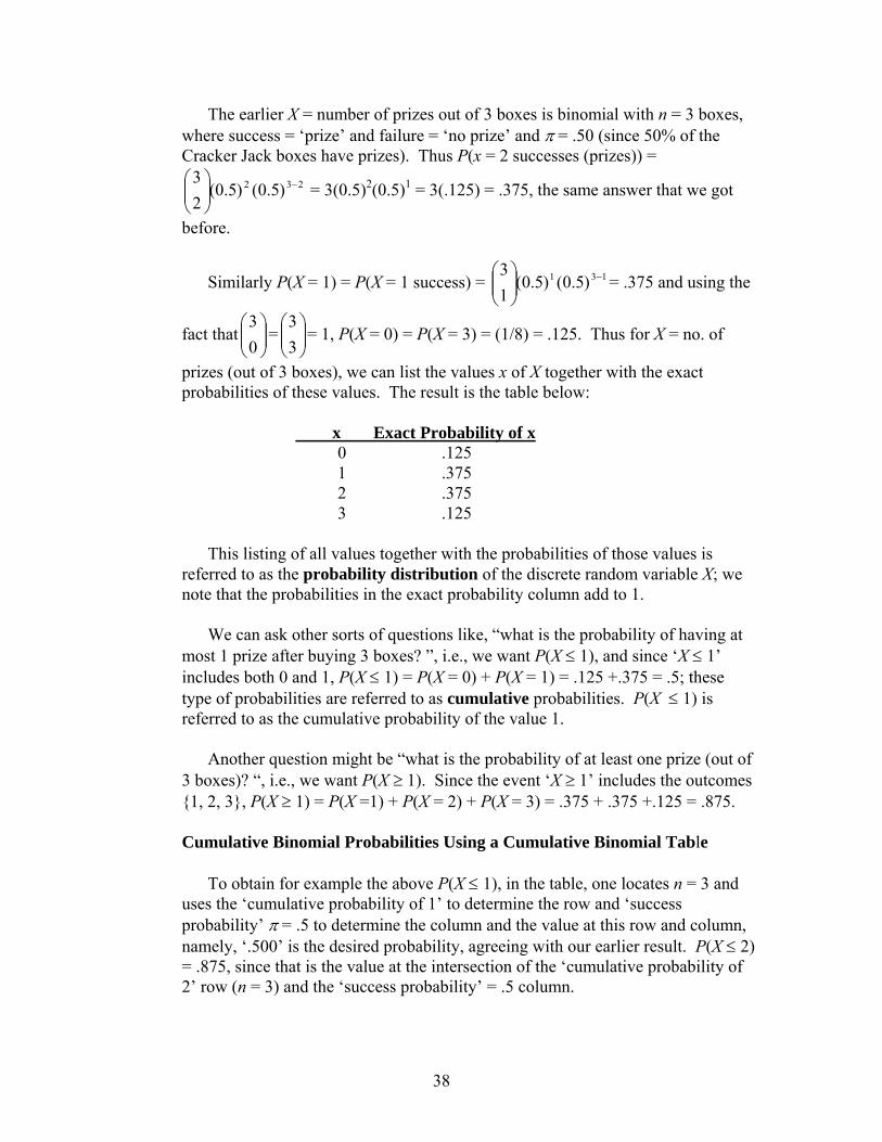
prizes (out of 3 boxes), we can list the values x of X together with the exact probabilities of these values. The result is the table below:

x Exact Probability of x

0 .125 1 .375 2 .375 3 .125

This listing of all values together with the probabilities of those values is referred to as the probability distribution of the discrete random variable X; we note that the probabilities in the exact probability column add to 1.

We can ask other sorts of questions like, “what is the probability of having at

most 1 prize after buying 3 boxes? ”, i.e., we want P(X ≤ 1), and since ‘X ≤ 1’ includes both 0 and 1, P(X ≤ 1) = P(X = 0) + P(X = 1) = .125 +.375 = .5; these type of probabilities are referred to as cumulative probabilities. P(X ≤ 1) is referred to as the cumulative probability of the value 1.

Another question might be “what is the probability of at least one prize (out of

3 boxes)? “, i.e., we want P(X ≥ 1). Since the event ‘X ≥ 1’ includes the outcomes {1, 2, 3}, P(X ≥ 1) = P(X =1) + P(X = 2) + P(X = 3) = .375 + .375 +.125 = .875.

Cumulative Binomial Probabilities Using a Cumulative Binomial Table

To obtain for example the above P(X ≤ 1), in the table, one locates n = 3 and uses the ‘cumulative probability of 1’ to determine the row and ‘success probability’ π = .5 to determine the column and the value at this row and column, namely, ‘.500’ is the desired probability, agreeing with our earlier result. P(X ≤ 2) = .875, since that is the value at the intersection of the ‘cumulative probability of 2’ row (n = 3) and the ‘success probability’ = .5 column.

39

Some textbooks contain cumulative binomial tables and some contain exact binomial tables (giving exact binomial probabilities just like the binomial formula); illustrated below are both types of tables.

Another Problem

Suppose that we randomly sample 15 boxes, where 80% of the entire

population of boxes have prizes. What is the probability that

(a) At most 11 of these boxes have prizes? (b) At least 12 of these boxes have prizes? (c) Exactly 12 of these boxes have prizes? Solution Using a Cumulative Binomial Table (a) P(X ≤ 11) = .352, the value at the intersection between the ‘cumulative

probability of 11’ row (n=15) and the ‘success probability’ = .80 column, since X = number of boxes (out of 15) with prizes is a binomial random variable with n = 15 and π =.80 (because of the 80% figure).

(b) P(X ≥ 12) = 1 − P(X ≤ 11) = 1 − .352 =.648, since when we subtract the

probability of {X ≤ 11} from the sum of all the probabilities (namely ‘1’), we remain with the probabilities of 12 or more. Another way to put it is that P(X ≥ 12) + P(X ≤ 11) = 1.

(c) P(X = 12) = P(X ≤ 12) − P(X ≤ 11) = .602 − .352 = .250. Why do you think

that subtracting the ‘12’ entry in the table from the ‘11’ entry gives the exact probability of 12?

Note that the P(X = 12) = 121512 )2.0()8.0(1215 −

⎟⎟⎠

⎞⎜⎜⎝

⎛= .250 from the binomial formula.

Solution Using an Exact Binomial Table

First note that X = number of boxes (out of 15) with prizes is a binomial

random variable with n = 15 and ‘success probability’ = .80 (because of the 80% figure).

(a) Locate the n=15 section of the table and then the ‘success probability’ (= .80)

column. Since the event {X ≤ 11} includes the exact values 0, 1, … ,11 of X, adding those probabilities together from the appropriate rows of the table (x = 0 through x = 11), results in P(X ≤ 11) = (.000 + .000 +… + .103 + .188) = .352.

40

(b) P(X ≥ 12) = 1 − P(X ≤ 11) = 1 − .352 =.648, since when we subtract the

probabilities of 0-11 from the sum of all the probabilities (namely ‘1’), we remain with the probabilities of 12 or more. Another way to put it is that P(X ≥ 12) + P(X ≤ 11) = 1. Alternatively, since the event {X ≥ 12} includes the exact values 12-20 of X, add those probabilities together from the appropriate rows of the table.

(c) P(X = 12) = ‘x = 12’ entry in the table = .250. Note that the P(X = 12) =

121512 )2.0()8.0(1215 −

⎟⎟⎠

⎞⎜⎜⎝

⎛= .250 from the binomial formula.

A 3rd Problem, this time without a solution

A machine consists of 5 components. Each component has a probability 0.9

of operating for a required period of time and we have independence between components, in terms of their successful operation (for the required period of time) or not. What is the probability that

(a) all 5 components operate successfully for the required period of time? (b) none of the components operate successfully for the required period of time? (c) exactly 3 of the components operate successfully for the required period of

time? (d) at least 3 of the components operate successfully for the required period of

time? (e) at most 2 of the components operate successfully for the required period of

time? (f) Suppose the machine works (for the required period of time) if at least 3 of the

components successfully operate. What is the probability that the machine works?

41

C. Population Mean μ and Population Standard deviation σ for a Discrete Random Variable

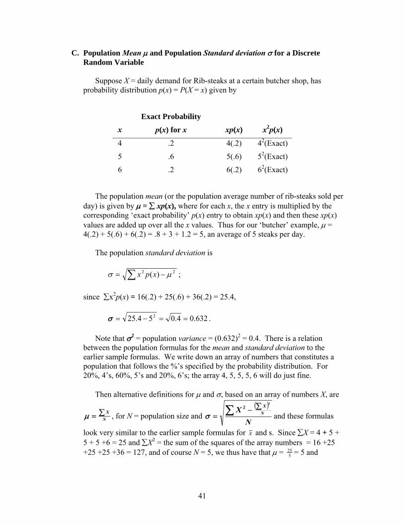
Suppose X = daily demand for Rib-steaks at a certain butcher shop, has

probability distribution p(x) = P(X = x) given by

x

Exact Probability

p(x) for x

xp(x)

x2p(x)

4 .2 4(.2) 42(Exact)

5 .6 5(.6) 52(Exact)

6 .2 6(.2) 62(Exact)

The population mean (or the population average number of rib-steaks sold per day) is given by μ = ∑ xp(x), where for each x, the x entry is multiplied by the corresponding ‘exact probability’ p(x) entry to obtain xp(x) and then these xp(x) values are added up over all the x values. Thus for our ‘butcher’ example, μ = 4(.2) + 5(.6) + 6(.2) = .8 + 3 + 1.2 = 5, an average of 5 steaks per day.

The population standard deviation is

∑ −= 22 )( μσ xpx ; since ∑x2p(x) = 16(.2) + 25(.6) + 36(.2) = 25.4,

632.04.054.25 2 ==−=σ .

Note that σ2 = population variance = (0.632)2 = 0.4. There is a relation between the population formulas for the mean and standard deviation to the earlier sample formulas. We write down an array of numbers that constitutes a population that follows the %’s specified by the probability distribution. For 20%, 4’s, 60%, 5’s and 20%, 6’s; the array 4, 5, 5, 5, 6 will do just fine.

Then alternative definitions for μ and σ, based on an array of numbers X, are

NX∑=μ , for N = population size and

( )

NX N

X∑ ∑−=

22

σ and these formulas

look very similar to the earlier sample formulas for x and s. Since ∑X = 4 + 5 + 5 + 5 +6 = 25 and ∑X2 = the sum of the squares of the array numbers = 16 +25 +25 +25 +36 = 127, and of course N = 5, we thus have that μ = 5

25 = 5 and

42

5127 5

252−=σ = 632.4.0

52

== . These answers are the same as our earlier

ones based on a probability distribution rather than on an array of numbers.

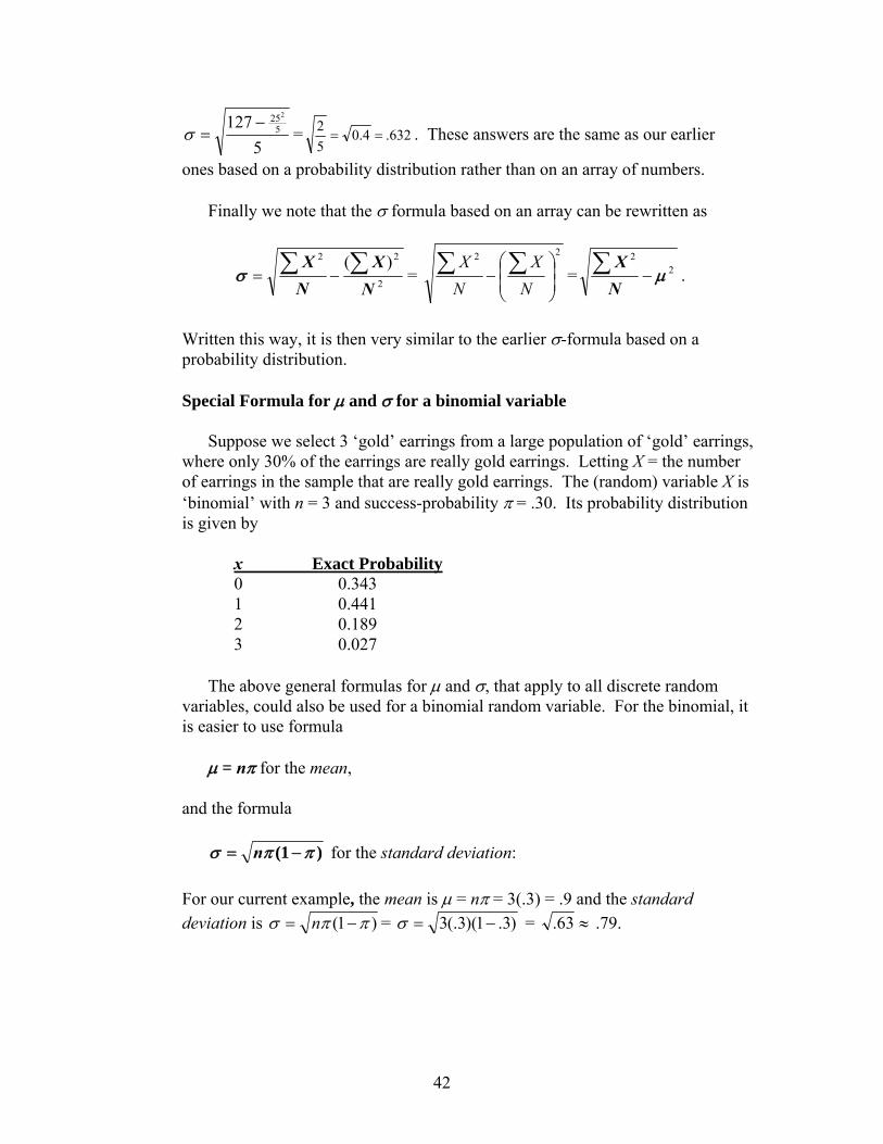
Finally we note that the σ formula based on an array can be rewritten as

2

22 )(N

XNX ∑∑ −=σ =

22

⎟⎟⎠

⎞⎜⎜⎝

⎛− ∑∑

NX

NX

= 22

μ−∑NX

.

Written this way, it is then very similar to the earlier σ-formula based on a probability distribution. Special Formula for μ and σ for a binomial variable

Suppose we select 3 ‘gold’ earrings from a large population of ‘gold’ earrings,

where only 30% of the earrings are really gold earrings. Letting X = the number of earrings in the sample that are really gold earrings. The (random) variable X is ‘binomial’ with n = 3 and success-probability π = .30. Its probability distribution is given by

x Exact Probability 0 0.343 1 0.441 2 0.189 3 0.027

The above general formulas for μ and σ, that apply to all discrete random

variables, could also be used for a binomial random variable. For the binomial, it is easier to use formula

μ = nπ for the mean,

and the formula

)1( ππσ −= n for the standard deviation: For our current example, the mean is μ = nπ = 3(.3) = .9 and the standard deviation is )1( ππσ −= n = )3.1)(3(.3 −=σ = ≈63. .79.

43

D. Hypergeometric (≡ Lotto-Like) Distribution

We have a population of size N containing S ‘success’ items and (N - S) ‘failure’ items. We randomly sample n items without replacement from this population. The probability that x of the success items appear in the sample is given by

P(x successes) = p(x) =

⎟⎟⎠

⎞⎜⎜⎝

⎛

⎟⎟⎠

⎞⎜⎜⎝

⎛−−

⎟⎟⎠

⎞⎜⎜⎝

⎛

nN

xnSN

xS

.

Note For the super-lotto lottery game discussed earlier, there are S = 6 player numbers out of the population of N = 52 numbers 1 – 52. n = 6 numbers are randomly selected from this population. To

determine the probability that exactly 5 player numbers are in the sample, substitute x = 5 in the above formula.

A Lotto-Like Problem

Three ‘gold’ earrings are randomly selected from a shipment containing 10 ‘gold’ earrings, altogether, with only 3 of the earrings being ‘real’ gold earrings. We are interested in the number of real gold earrings found in our sample of size 3.

(a) Identify ‘S’, ‘N’ and ‘n’ as defined above in the context of this current problem. (b) What is the probability that

(i) all 3 of the earrings in our sample are real gold? (ii) exactly 2 of the earrings in our sample are real gold?

NOTE: Since the earrings are selected without replacement, the probability

of (success, i.e. selecting a real gold earring) is not even approximately the same from one selection to the next but depends on results of previous selections. Thus the ‘independent trials’ assumption of the binomial is not satisfied and for this ‘small population’ example, an appropriate model is the ‘hypergeometric’ and not the ‘binomial’.

For example, the probability of choosing a real gold earring on the 1st

selection is (3/10), but given the information that real gold earrings were chosen on the 1st and 2nd selections, the probability of choosing a real gold earring on the 3rd selection is (1/8); this latter probability is very much different than (3/10) and thus the ‘independence’ assumption of the binomial model is not satisfied.

44

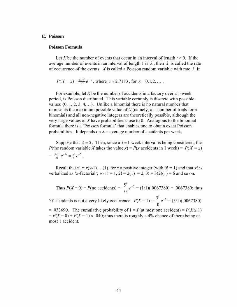
E. Poisson

Poisson Formula

Let X be the number of events that occur in an interval of length t > 0. If the average number of events in an interval of length 1 is λ , then λ is called the rate of occurrence of the events. X is called a Poisson random variable with rate λ if

( )

!( )xt t

xP X x eλ λ−= = , where 2.7183e ≈ , for 0,1, 2,x = … . For example, let X be the number of accidents in a factory over a 1-week

period, is Poisson distributed. This variable certainly is discrete with possible values {0, 1, 2, 3, 4,…}. Unlike a binomial there is no natural number that represents the maximum possible value of X (namely, n = number of trials for a binomial) and all non-negative integers are theoretically possible, although the very large values of X have probabilities close to 0. Analogous to the binomial formula there is a ‘Poisson formula’ that enables one to obtain exact Poisson probabilities. It depends on λ = average number of accidents per week.

Suppose that 5λ = . Then, since a 1t = week interval is being considered, the

P(the random variable X takes the value x) = P(x accidents in 1 week) = ( )P X x=

= ( ) 55! !

x xt tx xe eλ λ− −= .

Recall that x! = x(x-1)….(1), for x a positive integer (with 0! = 1) and that x! is

verbalized as ‘x-factorial’; so 1! = 1, 2! = 2(1) = 2, 3! = 3(2)(1) = 6 and so on.

Thus P(X = 0) = P(no accidents) = 50

!05 −e = (1/1)(.0067380) = .0067380; thus

‘0’ accidents is not a very likely occurrence. P(X = 1) = 51

!15 −e = (5/1)(.0067380)

= .033690. The cumulative probability of 1 = P(at most one accident) = P(X ≤ 1) = P(X = 0) + P(X = 1) ≈ .040; thus there is roughly a 4% chance of there being at most 1 accident.

45

Another Example, This one Illustrating the Cumulative and Exact Poisson Probability Tables

The number of failures per year of a certain type of copier is Poisson distributed with an average value of 10.

(a) What is the probability that the number of failures in a full year is

(i) At most 13? (ii) Exactly 10?

(b) What is the probability that the number of failures in a ½ year period is at least 2?

Solution using Tables First X = number of failures per year is Poisson with λ = 10.

(a) Using Cumulative Tables (i) P(X ≤ 13) = .8645 the value at the intersection between the x = 13 row

and λ = 10 column. (ii) P(X = 10) = .1251, the difference between .5830, the entry at the x =

10 row (corresponding to P(X ≤ 10) , of course still using the λ = 10 column), and .4579, the entry at the x = 9 column (corresponding to P(X ≤ 9) ).

(a) Using Exact Tables

(i) P(X ≤ 13) = .8645 the sum of the values at the intersections between the x = 0, 1, …, 13 rows and λ = 10 column.

(ii) P(X = 10) = .1251, the value at the intersection between the x = 10 row

and λ = 10 column.

Using your Favorite Table (b) One uses the 1

210( ) 5tλ = = column in the table, since this part of the question relates only to a ½ year period as opposed to a full year, as do the first two parts of the question. Then P(X ≥ 2) = 1 - .0404 = .9596 is the solution; note that .0404 corresponds to P(X ≤ 1) and gives us the same answer as gotten earlier using the Poisson formula.

46

F. Problems 1. A certain fried chicken retailer sends out discount coupons to individuals in a certain

population. Suppose it is believed that 36 % of the individuals in this population actually go out and make a purchase using these discount coupons. We randomly sample 8 individuals from this population. What is the probability that exactly 3 of them make a purchase using the coupons?

2. A general statement is made that an error occurs in 10% of all retail transactions. We

wish to evaluate the truthfulness of this figure for a particular retail store, say store A. Twenty transactions of this store are randomly obtained. Assuming that the 10% figure also applies to store A, evaluate the 'exact' probability that

(a) at most 2 of these transactions are in error? (b) at least 7 of these transactions are in error? (c) between 4 and 12 (inclusive of the endpoints) of these transactions are

in error?

3. Suppose that warranty records show that the probability that a new car needs a

warranty repair in the first 90 days is .05. In a sample of 10 new cars, what is the probability that in the first 90 days (a) None of them need a warranty repair?

(b) At most one needs a warranty repair?

(c) More than one needs a warranty repair?

47

4. 2% of the disk drives of a certain well-known brand fail within the first 90 days. In a sample of 5 disk drives, what is the probability that none of them fail within the first 90 days?

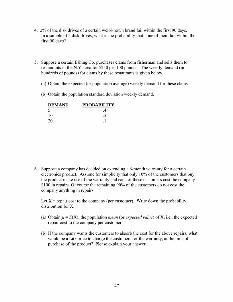
5. Suppose a certain fishing Co. purchases clams from fisherman and sells them to

restaurants in the N.Y. area for $250 per 100 pounds. The weekly demand (in hundreds of pounds) for clams by these restaurants is given below. (a) Obtain the expected (or population average) weekly demand for these clams.

(b) Obtain the population standard deviation weekly demand.

DEMAND PROBABILITY 5 .4 10 .5 20 . .1

6. Suppose a company has decided on extending a 6-month warranty for a certain

electronics product. Assume for simplicity that only 10% of the customers that buy the product make use of the warranty and each of these customers cost the company $100 in repairs. Of course the remaining 90% of the customers do not cost the

company anything in repairs

Let X = repair cost to the company (per customer). Write down the probability distribution for X.

(a) Obtain μ = E(X), the population mean (or expected value) of X, i.e., the expected

repair cost to the company per customer.

(b) If the company wants the customers to absorb the cost for the above repairs, what would be a fair price to charge the customers for the warranty, at the time of purchase of the product? Please explain your answer.

48

7. A manufacturer claims that 5% of her product is defective. If this claim is true, what is the probability that the number of defective products in a random sample of 20 will be

(a) Exactly 1? (b) At least 1?

Let X denote the number of defective products (out of 20); the possible values of X are then 0-20.

(c) Explain the rational behind the fact that the value ‘1’ has the highest probability

among the values 0-20.

(d) Obtain the population mean μ and the population standard deviation σ of X.

8. An individual is presented with 400 pairs of drinks, each pair consisting of one Pepsi

and one Coke in unmarked glasses. For each pair the individual must identify which of the drinks is the Coke. Assume that the individual has no skill and is just guessing. Let X = number of correct identifications (out of 400). Obtain the population mean μ and the population standard deviation σ of X.

Problems on the Poisson 9. Customers arrive at Sam’s used car lot at an average rate of 3 per hour. Suppose that

the number of customers arriving at his lot during any time period has a Poisson distribution.

(a) Find the probability that at most 2 customers arrive at Sam’s used car lot

during a given hour. (b) Find the probability that no customers arrive at Sam’s used car lot during

a given thirty minute period. (c) Find the probability that at least 2 but no more than 4 customers arrive at

Sam’s used car lot during a given thirty minute period.

49

10. Trucks arrive at a weighing station at a rate of 6 per hour. Suppose that the number

of trucks arriving at the weighing station during any time period has a Poisson distribution.

(a) Find the probability that at least 3 trucks arrive at the weighing station during a twenty-minute time period. (b) Find the probability that no trucks arrive at the weighing station during a ten minute time period. (c) Find the probability that more than 5 trucks arrive in a 40-minute time period.

Lotto-Like Problems

11. Problem on page 43 12. We randomly select 4 nursing homes from a population of 10 nursing homes,

where 4 are in violation of code and 6 are not. What is the probability that exactly 2 of the nursing homes in the sample are in violation of code?

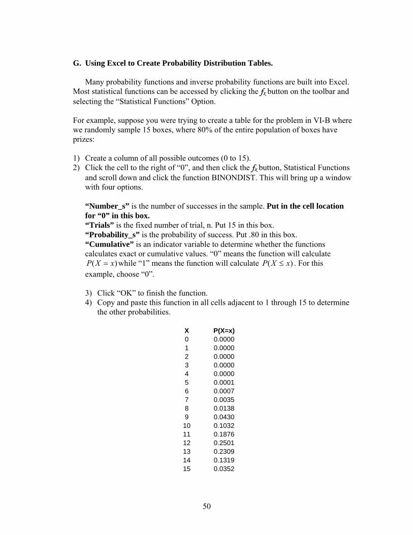
50

G. Using Excel to Create Probability Distribution Tables.

Many probability functions and inverse probability functions are built into Excel.

Most statistical functions can be accessed by clicking the fx button on the toolbar and selecting the “Statistical Functions” Option. For example, suppose you were trying to create a table for the problem in VI-B where we randomly sample 15 boxes, where 80% of the entire population of boxes have prizes: 1) Create a column of all possible outcomes (0 to 15). 2) Click the cell to the right of “0”, and then click the fx button, Statistical Functions

and scroll down and click the function BINONDIST. This will bring up a window with four options. “Number_s” is the number of successes in the sample. Put in the cell location for “0” in this box. “Trials” is the fixed number of trial, n. Put 15 in this box. “Probability_s” is the probability of success. Put .80 in this box. “Cumulative” is an indicator variable to determine whether the functions calculates exact or cumulative values. “0” means the function will calculate

)( xXP = while “1” means the function will calculate )( xXP ≤ . For this example, choose “0”. 3) Click “OK” to finish the function. 4) Copy and paste this function in all cells adjacent to 1 through 15 to determine

the other probabilities.

X P(X=x) 0 0.0000 1 0.0000 2 0.0000 3 0.0000 4 0.0000 5 0.0001 6 0.0007 7 0.0035 8 0.0138 9 0.0430 10 0.1032 11 0.1876 12 0.2501 13 0.2309 14 0.1319 15 0.0352

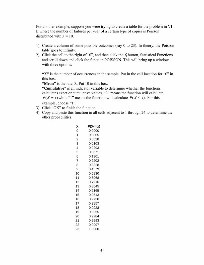
51

For another example, suppose you were trying to create a table for the problem in VI-E where the number of failures per year of a certain type of copier is Poisson distributed with λ = 10. 1) Create a column of some possible outcomes (say 0 to 23). In theory, the Poisson

table goes to infinity. 2) Click the cell to the right of “0”, and then click the fx button, Statistical Functions

and scroll down and click the function POISSON. This will bring up a window with three options. “X” is the number of occurrences in the sample. Put in the cell location for “0” in this box. “Mean” is the rate, λ. Put 10 in this box. “Cumulative” is an indicator variable to determine whether the functions calculates exact or cumulative values. “0” means the function will calculate

)( xXP = while “1” means the function will calculate )( xXP ≤ . For this example, choose “1”.

3) Click “OK” to finish the function. 4) Copy and paste this function in all cells adjacent to 1 through 24 to determine the

other probabilities.

X P(X<=x) 0 0.0000 1 0.0005 2 0.0028 3 0.0103 4 0.0293 5 0.0671 6 0.1301 7 0.2202 8 0.3328 9 0.4579

10 0.5830 11 0.6968 12 0.7916 13 0.8645 14 0.9165 15 0.9513 16 0.9730 17 0.9857 18 0.9928 19 0.9965 20 0.9984 21 0.9993 22 0.9997 23 1.0000

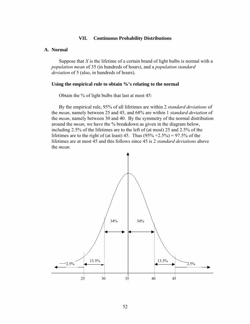
52

VII. Continuous Probability Distributions

A. Normal

Suppose that X is the lifetime of a certain brand of light bulbs is normal with a

population mean of 35 (in hundreds of hours), and a population standard deviation of 5 (also, in hundreds of hours).

Using the empirical rule to obtain %’s relating to the normal

Obtain the % of light bulbs that last at most 45: By the empirical rule, 95% of all lifetimes are within 2 standard deviations of

the mean, namely between 25 and 45, and 68% are within 1 standard deviation of the mean, namely between 30 and 40. By the symmetry of the normal distribution around the mean, we have the % breakdown as given in the diagram below, including 2.5% of the lifetimes are to the left of (at most) 25 and 2.5% of the lifetimes are to the right of (at least) 45. Thus (95% +2.5%) = 97.5% of the lifetimes are at most 45 and this follows since 45 is 2 standard deviations above the mean.

34% 34%

13.5%13.5%2.5% 2.5%

25 30 35 40 45

53

Obtain the % of light bulbs that last at most 30:

Since 30 is one standard deviation below the mean, (13.5% + 2.5%) = 16% of lifetimes are at most 30. Another way to reason is that 68% of the scores are within 1 standard deviation of the mean (between 30 and 40), and (100% - 32%) = 32% of the scores are outside of 30 – 40 (either below 30 or above 40). By symmetry, 16% = (32%/2) of the lifetimes fall below 30 and this is the desired answer.

We notice that the % of the lifetimes at most a certain value depend on how

many standard deviations the value is away from the mean, i.e., the ‘97.5%’ for a value of 45 is because 45 is 2 standard deviations above the mean and the ‘16%’ for a value of 30 is because 30 is 1 standard deviation below the mean. Using the empirical rule we are limited to whole numbered standard deviations like 1, 2 and 3. The Z table discussed below allows us to obtain results for scores that are not necessarily a whole number of standard deviations away from the mean.

Using the ‘CUMULATIVE’ standard normal (or Z) table to obtain normal %’s

We first differentiate between the actual score X that is observed called the

‘raw score’ and the number of standard deviations that X is away from the mean μ, referred to as the ‘Z score’ and is given by

σμ−

=XZ .

Thus a lifetime of X = 45 has a Z-value of Z = (45 – 35)/5 = 2, indicating that

X = 45 corresponds to a score that is 2 standard deviations above the mean. Also X = 30 has a corresponding Z score of Z = (30–35)/5 = -1 because ‘30’ is 1 standard deviation below the mean. To use the Z-table, one must work with the Z score rather the original X-score.

Obtain the % of light bulbs that last at most 45:

The cumulative % of 45 (the % of cases that are 45 or less) is given directly in the table, upon 1st obtaining the Z score of 45, namely Z = 2 = 2.00, locate the Z = ‘2.0’ row (corresponding to the whole number and tenths place value for Z) and the Z = ‘.00’ column (corresponding to the hundredths place for Z). The value found in the table at the intersection between above row and column, namely .9772, gives us the answer as a proportion. To obtain the desired %, simply multiply .9772 by 100 resulting in a value of 97.72%, slightly more accurate than our previous answer of 97.5% (where we used the empirical rule).

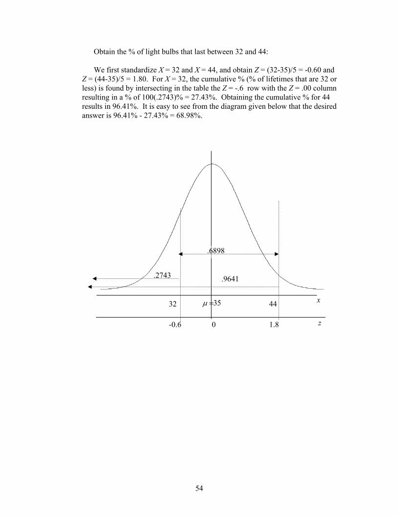
54

Obtain the % of light bulbs that last between 32 and 44: We first standardize X = 32 and X = 44, and obtain Z = (32-35)/5 = -0.60 and

Z = (44-35)/5 = 1.80. For X = 32, the cumulative % (% of lifetimes that are 32 or less) is found by intersecting in the table the Z = -.6 row with the Z = .00 column resulting in a % of 100(.2743)% = 27.43%. Obtaining the cumulative % for 44 results in 96.41%. It is easy to see from the diagram given below that the desired answer is 96.41% - 27.43% = 68.98%.

μ =35 x

z

32 44

0 -0.6 1.8

.9641.2743

.6898

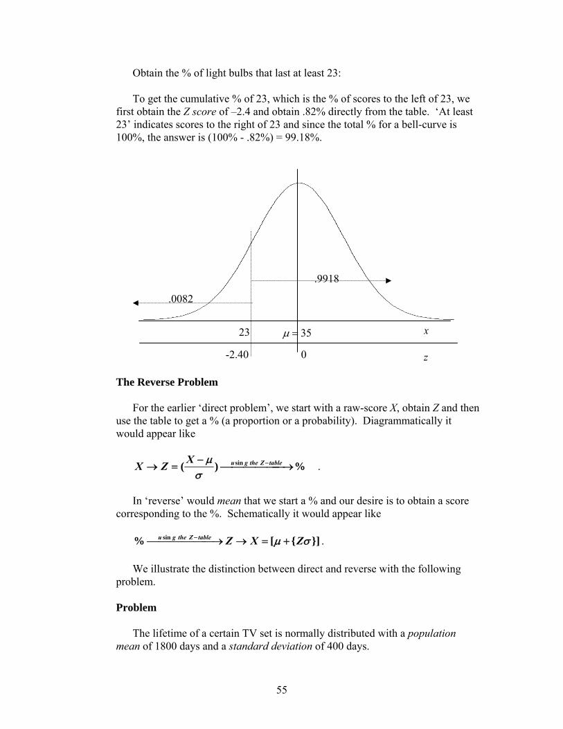
55

Obtain the % of light bulbs that last at least 23: To get the cumulative % of 23, which is the % of scores to the left of 23, we

first obtain the Z score of –2.4 and obtain .82% directly from the table. ‘At least 23’ indicates scores to the right of 23 and since the total % for a bell-curve is 100%, the answer is (100% - .82%) = 99.18%.

The Reverse Problem

For the earlier ‘direct problem’, we start with a raw-score X, obtain Z and then use the table to get a % (a proportion or a probability). Diagrammatically it would appear like

%)( sin ⎯⎯⎯⎯⎯ →⎯−

=→ −tableZtheguXZXσ

μ .

In ‘reverse’ would mean that we start a % and our desire is to obtain a score

corresponding to the %. Schematically it would appear like

}]{[% sin σμ ZXZtableZthegu +=→⎯⎯⎯⎯⎯ →⎯ − . We illustrate the distinction between direct and reverse with the following

problem. Problem

The lifetime of a certain TV set is normally distributed with a population mean of 1800 days and a standard deviation of 400 days.

μ = 35 x

z

23

0 -2.40

.0082

.9918

56

(a) What number of days corresponds to the 75th percentile? (b) What number of days corresponds to the 25th percentile? (c) Between what two numbers of days does the middle 50% of the distribution

lie? (d) If the company wants to guarantee the repairs of only 5% of the TV sets, how

long should the guarantee be? (e) What % of TV sets last at most 2900 days?

Solution Using the ‘CUMULATIVE’ standard normal (or Z) table. (a) We now look in the main body of the table and find the proportion entry

corresponding to ‘.75’ (= 75/100), or get as close as we can get to that value; in this case, ‘.7486’ is as close as we can get. We look to the margins to get the corresponding Z entry, both horizontally to get the whole number and the first decimal (in this case 0.6) and vertically to get the 2nd decimal (in this case .07), adding the two margin entries together gives us a Z-value of 0.67. This means for any normal curve for a score to be at the 75th percentile, it must lie approximately 2/3 of a standard deviation above the mean. The raw score X = # of days is then [1800+{0.67(400)}] = [1800+268] = 2068 days and this is the 75th percentile.

(b) Similarly looking up ‘.25’ in reverse in the main body of the table, results in a

Z-value of –0.67. A score at a percentile below 50 must be below the mean (since by symmetry the mean = median is at the 50th percentile) and this implies a negative Z score. The raw score X = # of days is then [1800-{0.67(400)}] = [1800-268] = 1532 days and this is the 25th percentile.

(c) By parts (a) and (b), the middle 50% of the lifetimes is between 1532 and 2068 (see the diagram given below). By symmetry of the normal curve around the mean, the number of days at the 75th and 25th percentiles are equally distant from the mean and have the same Z score in absolute value, except that the 25th has a Z score that is negative and the 75th has a Z score that is positive. This is true for any complementary percentiles (two percentiles adding to 100). Note that the percentile % is always the % to the left of the score; thus

X = 2068 has 25% of the lifetimes to the right of 2068 days but it is at the 75th percentile (and not the 25th) because 75% of the lifetimes are to the left of 2068.

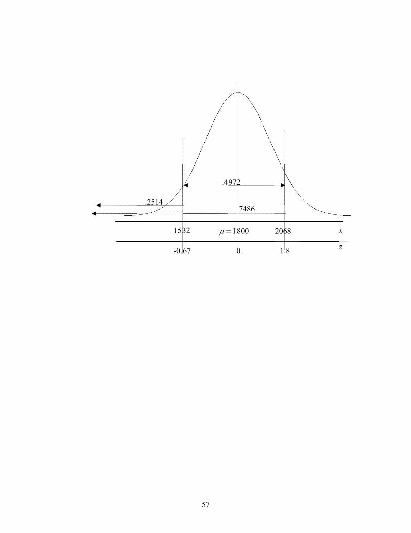
57

μ = 1800 x

z

1532 2068

0 -0.67 1.8

.7486.2514

.4972

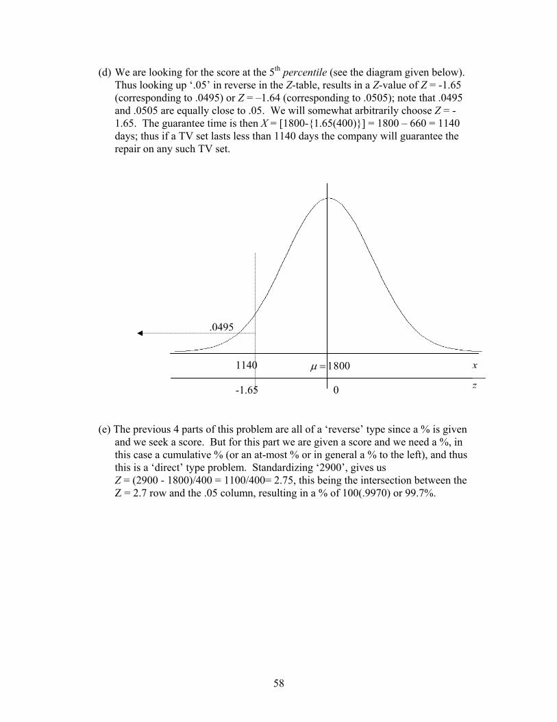
58

(d) We are looking for the score at the 5th percentile (see the diagram given below). Thus looking up ‘.05’ in reverse in the Z-table, results in a Z-value of Z = -1.65 (corresponding to .0495) or Z = –1.64 (corresponding to .0505); note that .0495 and .0505 are equally close to .05. We will somewhat arbitrarily choose Z = -1.65. The guarantee time is then X = [1800-{1.65(400)}] = 1800 – 660 = 1140 days; thus if a TV set lasts less than 1140 days the company will guarantee the repair on any such TV set.

(e) The previous 4 parts of this problem are all of a ‘reverse’ type since a % is given and we seek a score. But for this part we are given a score and we need a %, in this case a cumulative % (or an at-most % or in general a % to the left), and thus this is a ‘direct’ type problem. Standardizing ‘2900’, gives us Z = (2900 - 1800)/400 = 1100/400= 2.75, this being the intersection between the Z = 2.7 row and the .05 column, resulting in a % of 100(.9970) or 99.7%.

μ = 1800 x

z

1140

0 -1.65

.0495

59

B. Normal Approximation to the Binomial

For large sample sizes, the binomial random variable can be approximated by a bell-curve with population mean μ = nπ and population standard deviation σ = )1( ππ −n . This allows one to use the normal tables to evaluate binomial probabilities. Problem

A stockbroker claims to be able to make a successful deal on 30% of her calls. She plans to make 2100 calls over the next few months. Let X = number of successful deals out of 2100.

(a) Obtain the population mean and population standard deviation for X. (b) What is the probability of her making at least 670 successful deals out of the

2100 calls?

(c) Assuming X is approximately normal, obtain the symmetric interval of values (around the mean) that will contain the observed value of X with probability 0.88.

Solution

First X is binomial, where n = the number of her calls = 300 and π = probability of a successful deal (this would be labeled a ‘success’) = .30.

(a) The mean to be used is μ = 2100(.3) = 630 and the appropriate standard

deviation is σ = )3.1)(3(.2100 − = )7(.630 = 21. (b) Using the Cumulative Z table

The standardized score for X = 670 successful deals is evaluated as

Z = (X─ μ)/σ = (670─630)/21 = 1.90. We need now look up the area to the right of 1.90 in a standard normal table, resulting in (1- .9713) = .0287; note that ‘at least’ means to the right.

(c) This is a ‘reverse’ type problem. We 1st need the standardized value Z>0.

Then the area between –Z and Z is 0.88. Or equivalently, the area to the right of Z (as well as the area to the left of –Z) is (1─0.88)/2 = .06. Another way to look at it is that the area to the left of Z is 1 - .06 = .94.

Any way that one looks at it, using the cumulative standard normal tables

in reverse, with a value of .94, one obtains Z = 1.56 (or Z = 1.55). Finally the

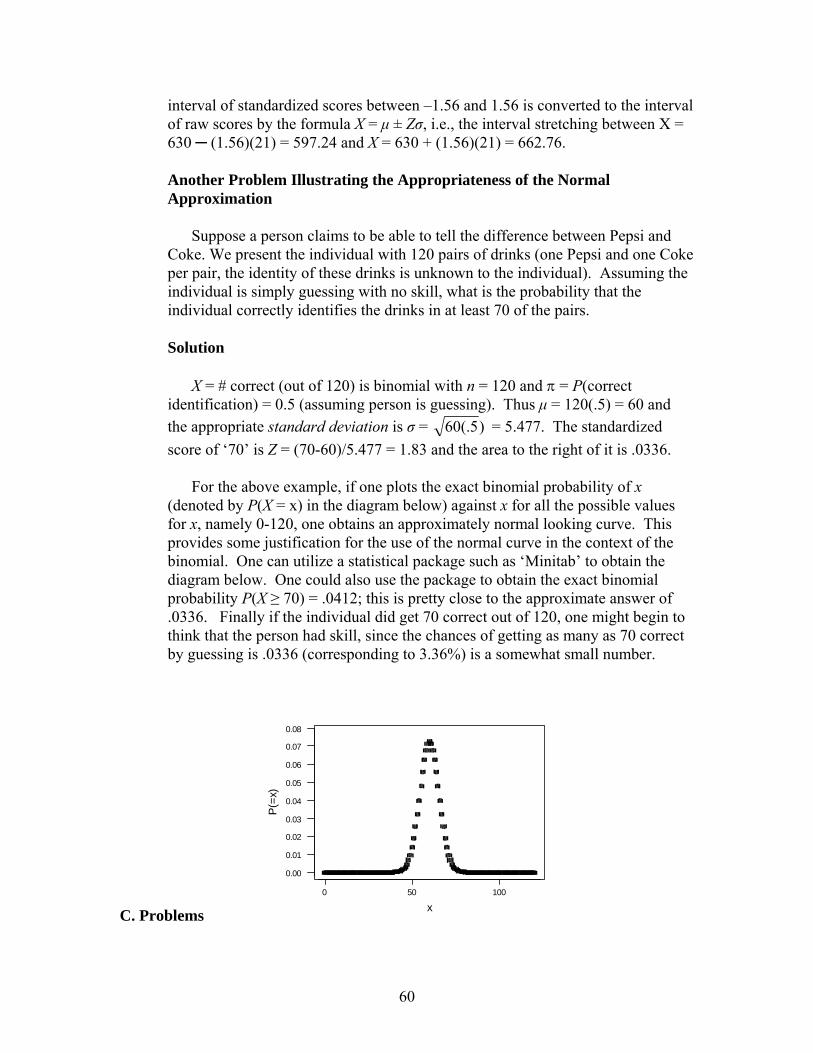
60

interval of standardized scores between –1.56 and 1.56 is converted to the interval of raw scores by the formula X = μ ± Zσ, i.e., the interval stretching between X = 630 ─ (1.56)(21) = 597.24 and X = 630 + (1.56)(21) = 662.76.

Another Problem Illustrating the Appropriateness of the Normal Approximation

Suppose a person claims to be able to tell the difference between Pepsi and Coke. We present the individual with 120 pairs of drinks (one Pepsi and one Coke per pair, the identity of these drinks is unknown to the individual). Assuming the individual is simply guessing with no skill, what is the probability that the individual correctly identifies the drinks in at least 70 of the pairs. Solution

X = # correct (out of 120) is binomial with n = 120 and π = P(correct identification) = 0.5 (assuming person is guessing). Thus μ = 120(.5) = 60 and the appropriate standard deviation is σ = )5(.60 = 5.477. The standardized score of ‘70’ is Z = (70-60)/5.477 = 1.83 and the area to the right of it is .0336.

For the above example, if one plots the exact binomial probability of x

(denoted by P(X = x) in the diagram below) against x for all the possible values for x, namely 0-120, one obtains an approximately normal looking curve. This provides some justification for the use of the normal curve in the context of the binomial. One can utilize a statistical package such as ‘Minitab’ to obtain the diagram below. One could also use the package to obtain the exact binomial probability P(X ≥ 70) = .0412; this is pretty close to the approximate answer of .0336. Finally if the individual did get 70 correct out of 120, one might begin to think that the person had skill, since the chances of getting as many as 70 correct by guessing is .0336 (corresponding to 3.36%) is a somewhat small number.

C. Problems

100500

0.08

0.07

0.06

0.05

0.04

0.03

0.02

0.01

0.00

x

P(=x

)

61

1. A normally distributed population of package weights has a mean of 63.5 g and a standard deviation of 12.2 g.

(a) What percentage of this population weighs 78.0 g or more? (b) What percentage of this population weighs 41.0 g or less? (c) What percentage of this population weigh between 41.0 g and 78g? (d) 88% of all package weights fall in some interval that is symmetric about 63.5, the

population mean. Obtain this interval. 2. Plastic bags used for packaging produce are manufactured so that the breaking

strength of the bag is normally distributed with a mean of 5 pounds per square inch and a standard deviation of 1.5 pounds per square inch.

(a) What proportion of the bags produced have a breaking strength of

(1) At least 3.6 pounds per square inch? (2) At most 3.17 pounds per square inch?

(b) Obtain the breaking strength at the 57th percentile. (c) Between what two values symmetrically distributed around the mean will

95% of the breaking strengths fall?

3. The score on an application test for employment at a particular company is normally distributed with a population mean μ = 75 and a population standard deviation σ = 8.

(a) What percentage of the applicants who take the test score

(I) Between 71 and 87? (II) At least 87?

(b) What is the cumulative % of a score of 92? (c) How high must an individual score to be at the 99th percentile?

62

4. Suppose that the monthly bills of a network company’s customers have a normal

distribution with a mean of $53 and standard deviation of $15.

a. If one of these bills is selected at random, then what is the probability that it is at most $70? b. Find the 75th percentile of these bills.

5. Suppose that Harry’s utility bills have a normal distribution with a mean of $87 and a standard deviation of $13.

a. Find the probability that his utility bill is between $80 and $100.

b. Thirty percent of his utility bills are larger than what amount?

6. Suppose that the weights of shipments at a loading dock have a normal distribution with a mean of 3.4 tons and a standard deviation of 1.1 tons.

a. Suppose that a shipment at the loading dock is selected at random. Find

the probability that the shipment has a weight of at most 4.6 tons. b. Thirty-three percent of the shipments have weight that is at most what

amount?

63

Problems on the Normal Approximation to the binomial 7. A certain fried chicken retailer sends out discount coupons to individuals in a certain

population. Suppose it is believed that 36 % of the individuals in this population actually go out and make a purchase using these discount coupons. We randomly sample 2500 from the population. Let X = number of people in the sample of 2500 who make a purchase using the coupons.

(a) It can be shown that X is approximately normal with population

mean = 900 and population standard deviation = 24. Write down the formulas needed to obtain the above values of the mean and standard deviation and evaluate them to obtain the above results.

(b) Obtain the probability that at least 940 out of our sample of 2500 use

the coupons?

(c) Obtain the 98th percentile for X, i.e., we need a certain ‘value’ so that there is a 98 % chance that X is at most that ‘value’.

(d) Suppose it turned out that 960 people in our sample used the

coupons, i.e., we observed X = 960, would that outcome make one suspicious of the 36 % population figure for people making purchases. Please explain.

8. Suppose that it is known from a great deal of record keeping that 50% of TV viewers react positively to a certain advertisement. We randomly sample 10,000 of these viewers. Let X = number of viewers (out of 10,000) that react positively to the advertisement.

(a) Obtain the population mean and population standard deviation of X. (b) Assuming X is approximately normal, obtain the symmetric interval of values

(around the mean) that will contain the observed value of X with probability 0.94. (c) If one observed an X value of 4950,would this cast doubt on the population figure

and indicate that the true population % should be less than 50? Please explain your answer to this question by making use of your answer to part (b).

(d) What is the probability that X is at least 4900?

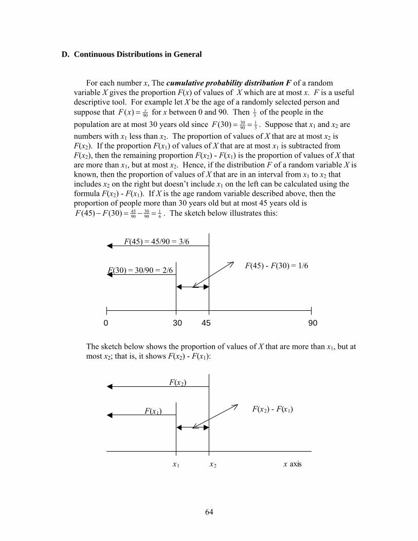
64

D. Continuous Distributions in General

For each number x, The cumulative probability distribution F of a random variable X gives the proportion F(x) of values of X which are at most x. F is a useful descriptive tool. For example let X be the age of a randomly selected person and suppose that 90( ) xF x = for x between 0 and 90. Then 1

3 of the people in the population are at most 30 years old since 30 1

90 3(30)F = = . Suppose that x1 and x2 are numbers with x1 less than x2. The proportion of values of X that are at most x2 is F(x2). If the proportion F(x1) of values of X that are at most x1 is subtracted from F(x2), then the remaining proportion F(x2) - F(x1) is the proportion of values of X that are more than x1, but at most x2. Hence, if the distribution F of a random variable X is known, then the proportion of values of X that are in an interval from x1 to x2 that includes x2 on the right but doesn’t include x1 on the left can be calculated using the formula F(x2) - F(x1). If X is the age random variable described above, then the proportion of people more than 30 years old but at most 45 years old is

45 30 190 90 6(45) (30)F F− = − = . The sketch below illustrates this:

F(45) - F(30) = 1/6

30 0

F(45) = 45/90 = 3/6

F(30) = 30/90 = 2/6

45 90

The sketch below shows the proportion of values of X that are more than x1, but at most x2; that is, it shows F(x2) - F(x1):

F(x2) - F(x1)

x1

F(x2)

F(x1)

x2 x axis

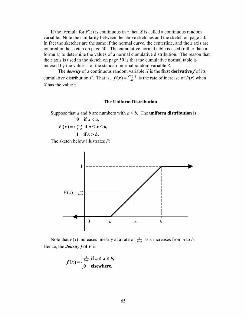
65

If the formula for F(x) is continuous in x then X is called a continuous random variable. Note the similarity between the above sketches and the sketch on page 50. In fact the sketches are the same if the normal curve, the centerline, and the z axis are ignored in the sketch on page 50. The cumulative normal table is used (rather than a formula) to determine the values of a normal cumulative distribution. The reason that the z axis is used in the sketch on page 50 is that the cumulative normal table is indexed by the values z of the standard normal random variable Z.

The density of a continuous random variable X is the first derivative f of its cumulative distribution F. That is, ( )( ) dF x

dxf x = is the rate of increase of F(x) when X has the value x.

The Uniform Distribution Suppose that a and b are numbers with a < b. The uniform distribution is

0 if ,

( ) if ,1 if .

x ab a

x aF x a x b

x b

−−

<⎧⎪= ≤ ≤⎨⎪ >⎩

The sketch below illustrates F:

1

a b 0 x

( ) x ab aF x −

−=

Note that F(x) increases linearly at a rate of 1

b a− as x increases from a to b. Hence, the density f of F is

1 if ,

( )0 elsewhere.b a a x b

f x − ≤ ≤⎧= ⎨

⎩

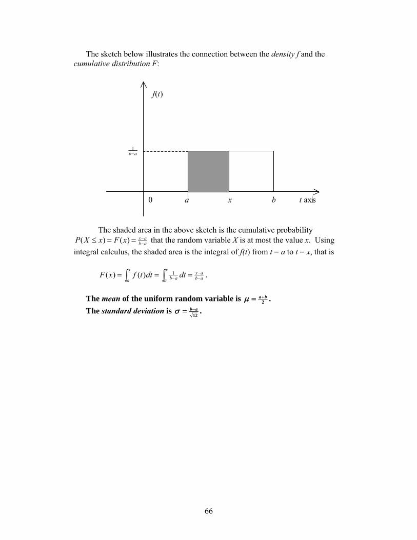
66

The sketch below illustrates the connection between the density f and the cumulative distribution F:

a b 0 x

f(t)

t axis

1b a−

The shaded area in the above sketch is the cumulative probability

( ) ( ) x ab aP X x F x −

−≤ = = that the random variable X is at most the value x. Using integral calculus, the shaded area is the integral of f(t) from t = a to t = x, that is

1( ) ( )

x xx a

b a b aa aF x f t dt dt −

− −= = =∫ ∫ .

The mean of the uniform random variable is 2

a bμ += . The standard deviation is

12b aσ −= .

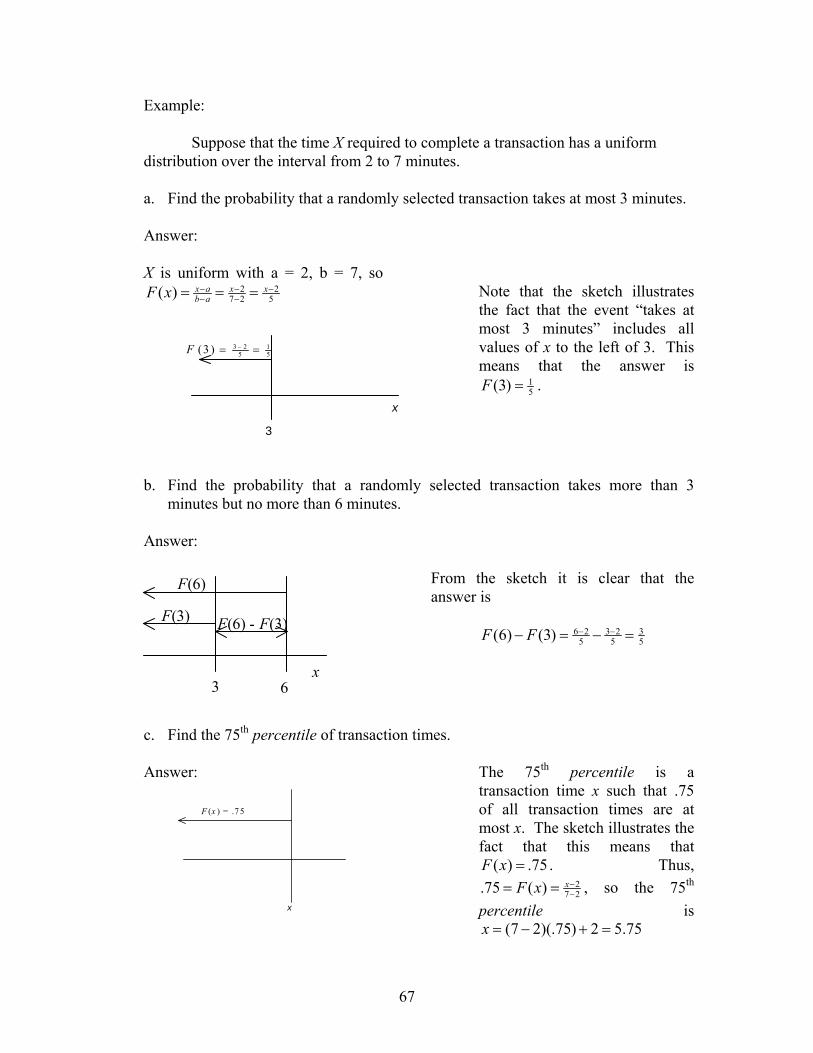
67

Example: Suppose that the time X required to complete a transaction has a uniform

distribution over the interval from 2 to 7 minutes.

a. Find the probability that a randomly selected transaction takes at most 3 minutes.

Answer: X is uniform with a = 2, b = 7, so

2 27 2 5( ) x a x x

b aF x − − −− −= = =

3

x

3 2 15 5(3 )F −= =

Note that the sketch illustrates the fact that the event “takes at most 3 minutes” includes all values of x to the left of 3. This means that the answer is

15(3)F = .

b. Find the probability that a randomly selected transaction takes more than 3

minutes but no more than 6 minutes.

Answer:

3 6 x

F(3)

F(6)

F(6) - F(3)

From the sketch it is clear that the answer is

6 2 3 2 3

5 5 5(6) (3)F F − −− = − =

c. Find the 75th percentile of transaction times. Answer:

x

F (x ) = .75

The 75th percentile is a transaction time x such that .75 of all transaction times are at most x. The sketch illustrates the fact that this means that

( ) .75F x = . Thus, 2

7 2.75 ( ) xF x −−= = , so the 75th

percentile is (7 2)(.75) 2 5.75x = − + =

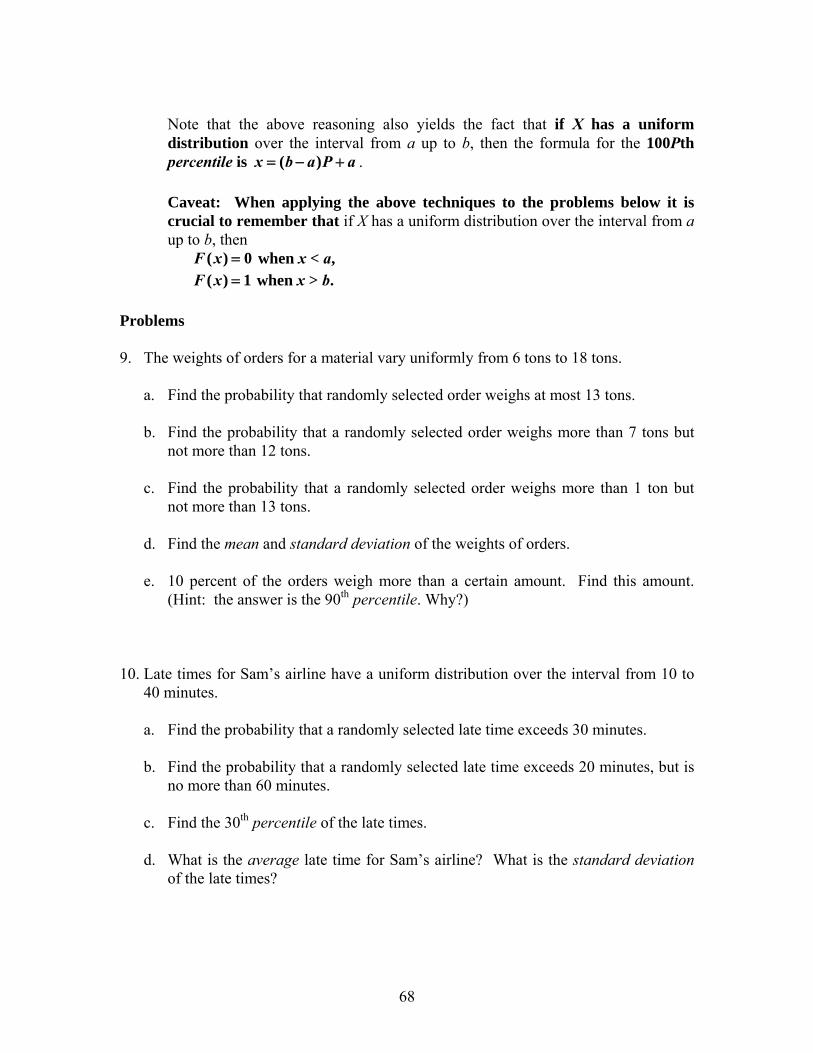
68

Note that the above reasoning also yields the fact that if X has a uniform distribution over the interval from a up to b, then the formula for the 100Pth percentile is ( )x b a P a= − + . Caveat: When applying the above techniques to the problems below it is crucial to remember that if X has a uniform distribution over the interval from a up to b, then ( ) 0F x = when x < a,

( ) 1F x = when x > b.

Problems

9. The weights of orders for a material vary uniformly from 6 tons to 18 tons.

a. Find the probability that randomly selected order weighs at most 13 tons. b. Find the probability that a randomly selected order weighs more than 7 tons but

not more than 12 tons.

c. Find the probability that a randomly selected order weighs more than 1 ton but not more than 13 tons.

d. Find the mean and standard deviation of the weights of orders.

e. 10 percent of the orders weigh more than a certain amount. Find this amount.

(Hint: the answer is the 90th percentile. Why?)

10. Late times for Sam’s airline have a uniform distribution over the interval from 10 to

40 minutes.

a. Find the probability that a randomly selected late time exceeds 30 minutes. b. Find the probability that a randomly selected late time exceeds 20 minutes, but is

no more than 60 minutes.

c. Find the 30th percentile of the late times.

d. What is the average late time for Sam’s airline? What is the standard deviation of the late times?

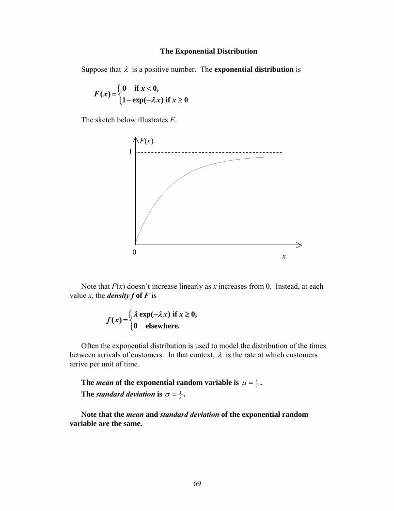
69

The Exponential Distribution

Suppose that λ is a positive number. The exponential distribution is

0 if 0,

( )1 exp( ) if 0

xF x

x xλ<⎧

= ⎨ − − ≥⎩

The sketch below illustrates F.

1 F(x)

x 0

Note that F(x) doesn’t increase linearly as x increases from 0. Instead, at each

value x, the density f of F is

exp( ) if 0,( )

0 elsewhere.x x

f xλ λ− ≥⎧

= ⎨⎩

Often the exponential distribution is used to model the distribution of the times

between arrivals of customers. In that context, λ is the rate at which customers arrive per unit of time.

The mean of the exponential random variable is 1

λμ = . The standard deviation is 1

λσ = . Note that the mean and standard deviation of the exponential random

variable are the same.

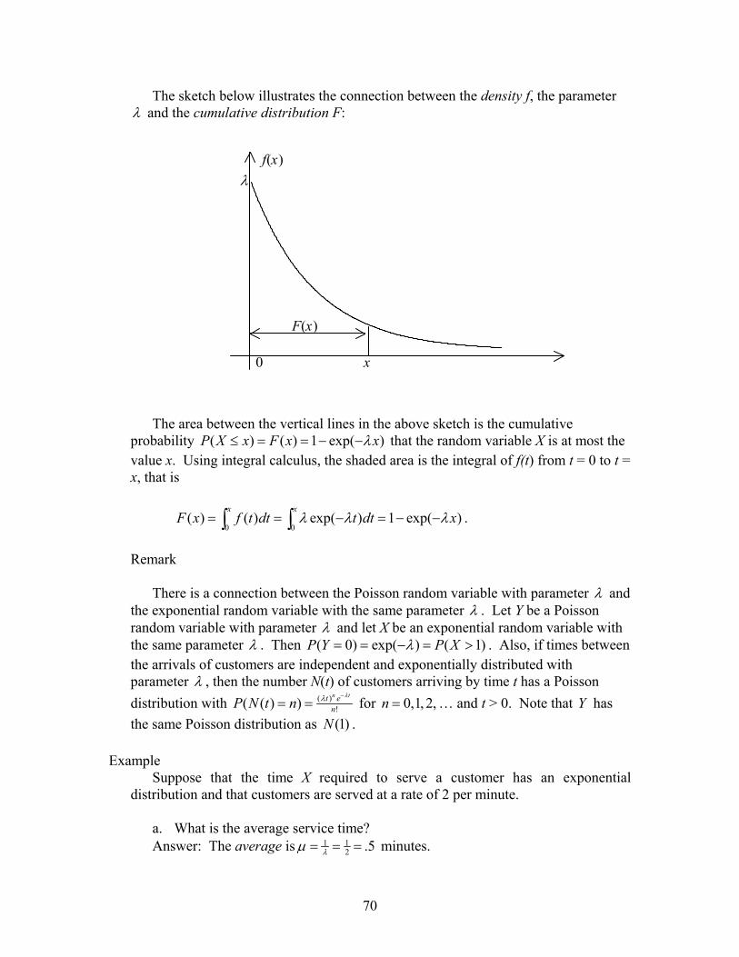
70

The sketch below illustrates the connection between the density f, the parameter λ and the cumulative distribution F:

x

F(x)

0

f(x) λ

The area between the vertical lines in the above sketch is the cumulative

probability ( ) ( ) 1 exp( )P X x F x xλ≤ = = − − that the random variable X is at most the value x. Using integral calculus, the shaded area is the integral of f(t) from t = 0 to t = x, that is

0 0( ) ( ) exp( ) 1 exp( )

x xF x f t dt t dt xλ λ λ= = − = − −∫ ∫ .

Remark

There is a connection between the Poisson random variable with parameter λ and

the exponential random variable with the same parameter λ . Let Y be a Poisson random variable with parameter λ and let X be an exponential random variable with the same parameter λ . Then ( 0) exp( ) ( 1)P Y P Xλ= = − = > . Also, if times between the arrivals of customers are independent and exponentially distributed with parameter λ , then the number N(t) of customers arriving by time t has a Poisson distribution with ( )

!( ( ) )n tt enP N t n

λλ −

= = for 0,1, 2,n = … and t > 0. Note that Y has the same Poisson distribution as (1)N .

Example

Suppose that the time X required to serve a customer has an exponential distribution and that customers are served at a rate of 2 per minute.

a. What is the average service time?

Answer: The average is 1 12 .5λμ = = = minutes.

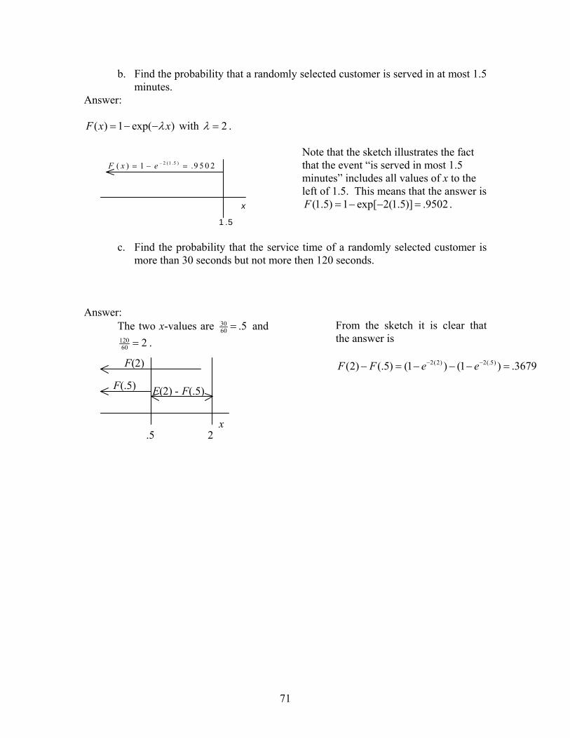
71

b. Find the probability that a randomly selected customer is served in at most 1.5 minutes.

Answer:

( ) 1 exp( )F x xλ= − − with 2λ = .

1 .5

x

2 (1 .5 )( ) 1 .9 5 0 2F x e −= − =

Note that the sketch illustrates the fact that the event “is served in most 1.5 minutes” includes all values of x to the left of 1.5. This means that the answer is

(1.5) 1 exp[ 2(1.5)] .9502F = − − = .

c. Find the probability that the service time of a randomly selected customer is

more than 30 seconds but not more then 120 seconds.

Answer:The two x-values are 30

60 .5= and 12060 2= .

.5 2 x

F(.5)

F(2)

F(2) - F(.5)

From the sketch it is clear that the answer is

2(2) 2(.5)(2) (.5) (1 ) (1 ) .3679F F e e− −− = − − − =

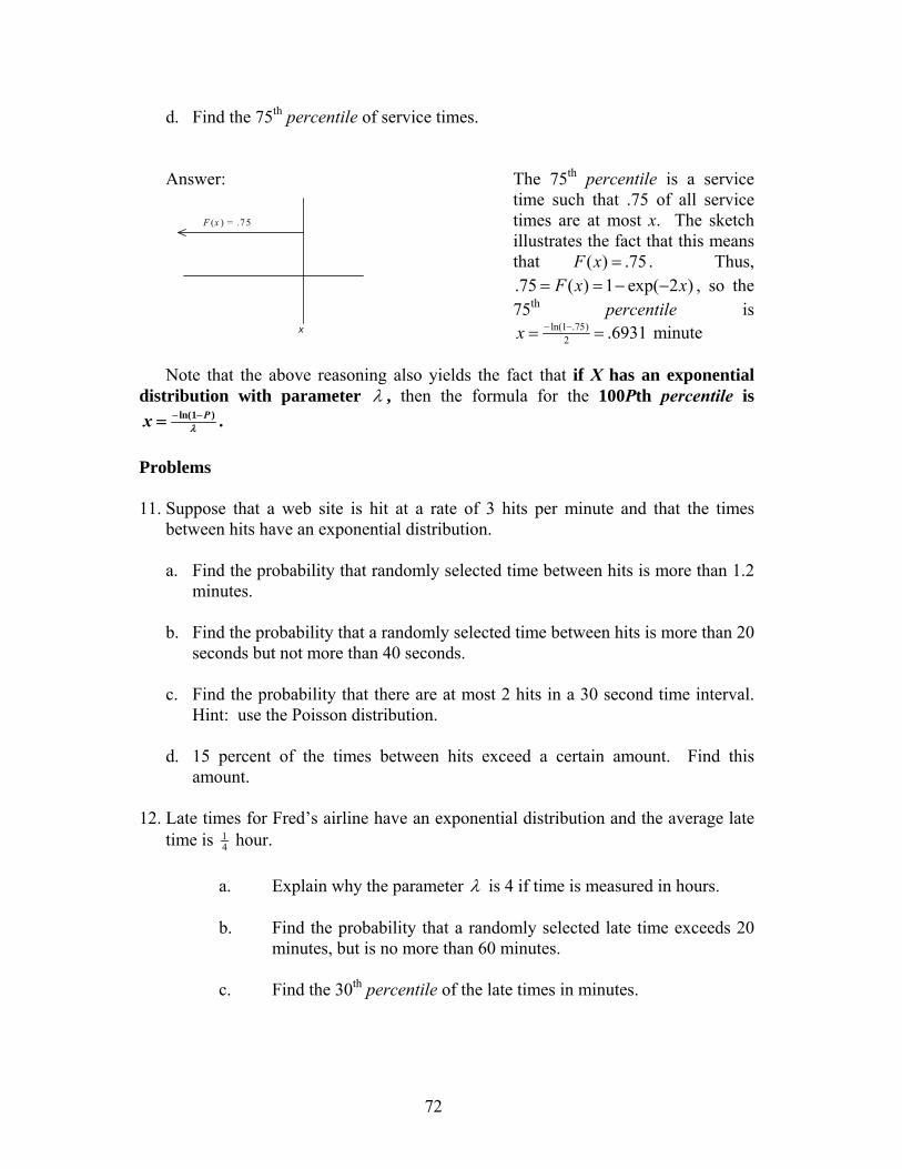
72

d. Find the 75th percentile of service times.

Answer:

x

F (x ) = .75

The 75th percentile is a service time such that .75 of all service times are at most x. The sketch illustrates the fact that this means that ( ) .75F x = . Thus, .75 ( ) 1 exp( 2 )F x x= = − − , so the 75th percentile is

ln(1 .75)2 .6931x − −= = minute

Note that the above reasoning also yields the fact that if X has an exponential distribution with parameter λ , then the formula for the 100Pth percentile is

ln(1 )Px λ− −= .

Problems

11. Suppose that a web site is hit at a rate of 3 hits per minute and that the times

between hits have an exponential distribution. a. Find the probability that randomly selected time between hits is more than 1.2

minutes. b. Find the probability that a randomly selected time between hits is more than 20

seconds but not more than 40 seconds.

c. Find the probability that there are at most 2 hits in a 30 second time interval. Hint: use the Poisson distribution.

d. 15 percent of the times between hits exceed a certain amount. Find this

amount.

12. Late times for Fred’s airline have an exponential distribution and the average late time is 1

4 hour.

a. Explain why the parameter λ is 4 if time is measured in hours. b. Find the probability that a randomly selected late time exceeds 20

minutes, but is no more than 60 minutes. c. Find the 30th percentile of the late times in minutes.

73

E. Using Excel to find Normal Probabilities and Percentiles

The Normal probability function (NORMDIST) and inverse probability function

(NORMINV) is built into Excel. Click the fx button on the toolbar, select the “Statistical Functions” Option and scroll down to the appropriate function. In the example from VII-A, X is the lifetime of a certain brand of light bulbs is normal with a population mean of 35 (in hundreds of hours), and a population standard deviation of 5 (also, in hundreds of hours). To find )45( <XP : Highlight any cell and click the fx button, Statistical Functions and scroll down

and click the function NORMDIST. Set “X” equal to 45. Set “Mean” equal to 35.

Set “Standard_Dev” equal to 5. Set “Cumulative” equal to 1. The function returns 9772.)45( =<XP

In the example from VII-A, the lifetime of a certain TV set is normally distributed with a population mean of 1800 days and a standard deviation of 400 days. To find the 75th percentile of the TV set lifetimes:

Highlight any cell and click the fx button, Statistical Functions and scroll down and click the function NORMINV. Set “Probability” equal to 0.75, the percentile of interest. Set “Mean” equal to 1800.

Set “Standard_Dev” equal to 400. The function returns the 75th percentile = 2070 days.

74

VIII. Background for Inference

Let X = rating for the movie ‘Antz’ on a scale from 0-100. Over a certain

population let μ = population mean rating for the movie and let σ = the population standard deviation. If X were normally distributed then for approximately 95% of the ratings in the population X = μ ± 2σ, i.e., X is between μ − 2σ and μ + 2σ.

Thus, for example, if μ = 80 and σ = 6, and X were normal, 95% of the ratings

in the population would be between 80−2(6) and 80+2(6) or between 68 and 92. If n ratings were randomly gotten from the population, then according to an extremely important theorem called the ‘Central Limit Theorem’, the distribution of X , the sample average, is approximately normal for large n; this is true even if the original X data is non-normal.

The reasoning behind the theorem is that any outlying X scores (which

although infrequent do occur, especially for non-normal data) are dampened by averaging over mainly moderate scores, resulting almost always in moderate values of X . It can also be shown that for n independent observations, X has mean μ, the same as for a single observation, but standard deviation given by

nXσσ = .

There is less variation between one sample average and another then there is

between one single rating and another and the variability in the sample average goes down as the sample size n goes up. Thus for large n, X is approximately normal with mean μ and standard deviation

nσ (as given above); therefore, with

probability .95, n

X σμ 2between is ± . For the above Antz example, based on a sample of size 81 (considered large),

with probability .95, 816280between is ±X or equivalently, X is between 80 ±

1.33, or finally X is between 78.67 and 81.33. Background for the Inference Formula on the Next Page

Verbalizing the import of the latter part of the last paragraph as “ for a large sample, with 95% confidence (or with probability .95), X differs from μ by at most

nσ2 ,” inferences about the unknown population mean μ can now be made.

Suppose ‘It’s a bug’s life’ is also being rated on a scale from 0-100 but now

the population mean rating is not known as it was for ‘Antz’ (but it is known that the population standard deviation σ = 7). We sample 100 individuals from the population and have them rate ‘It’s a Bug’s Life’ and obtain a sample average of

75

90. It is then concluded with 95% confidence that 90=X differs from μ by at most .4.122

1007 ==

nσ

Thus with 95% confidence

nX σμ 2between is ± or equivalently

4.190between is ±μ or finally that μ is between 90 - 1.4 = 88.6 and 90 + 1.4 = 91.4. The interval for μ between 88.6 and 91.4 is referred to as a 95% confidence interval.

The general statement “

nX σμ 2between is ± ” is now used again to obtain a

large sample 95% confidence interval. We now remove the impractical part of the above statement, the fact that we need to know σ, by replacing it by s = sample standard deviation, which can be calculated from the data. Since we are dealing with a large sample, s is not far from σ, and thus the above formula is replaced by the more practical “

nsX 2between is ±μ ”.

We illustrate the formula in its present form by the following example. It is

our desire to check out advertised 100-ounce containers of liquid cheer and to ensure that at least on the average they contain what they are supposed to, namely 100ozs. 64 such containers are sampled and a sample average X , and a sample standard deviation are obtained as X = 99.95, s = 0.4.

The 95% confidence interval for the average number μ of ounces per

container has limits644.295.99 ± or that μ is between (99.95-0.1) = 99.85 and

(99.95+0.1) = 100.05 with 95% confidence. We thus cannot reject the 100 oz advertised amount since it falls in the

confidence interval. If we had observed X = 99. 5 and s = 0.4, then our 95% confidence interval would have been 99.4 ≤ μ ≤ 99.6 and 100 oz’s would have been rejected as the population average per container (with 95% confidence), since ‘100’ now falls outside of the confidence interval, with ’99.6’ now being the upper endpoint of the interval.

With 95% confidence, one could thus conclude that the public was being

shortchanged by at least (100-99.6) = 0.4 oz’s per container. For the above formula we have used ‘2’ to correspond to the 95% confidence level. Below the formula is generalized to allow for more general confidence levels.

76

IX. One Sample Inference: Quantitative Data

A. Confidence Intervals for a population mean: Large & Small Sample

Confidence Intervals, Large

The formula for a large sample confidence interval (abbreviated as CI), is given by

nszx c±=μ ,

where averagex sample= , s = sample standard deviation and n = sample size ( ≥ 30 for the large sample problems) and where cz > 0 is chosen so that the % under a standard normal curve between - cz and + cz is equal to the specified confidence %, i.e., so that the middle % under a standard normal curve is equal to

the confidence %. We note that the above ‘±’ amount nszc is referred to as the

margin of error (say, E).

Determination of the sample size n:

One can also set the confidence level at some % and set the margin of

error E at some desired amount and use the equation nszE c= to solve for n

resulting in

2

⎟⎠

⎞⎜⎝

⎛=E

szn c

We illustrate the above with the following problem.

Problem

Last year, the average December residential heating bill was $93.41. A random sample of 41 residential heating bills has a mean amount of $96.52 with a standard deviation of $10.34.

(a) Obtain a 95% CI for the current year population average residential bill. (b) Does this information contained in the CI indicate that the average residential

heating bill has changed?

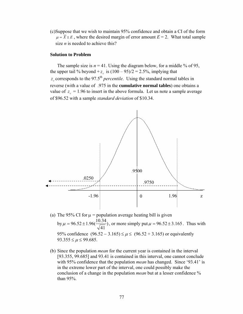
77

(c) Suppose that we wish to maintain 95% confidence and obtain a CI of the form EX ±=μ , where the desired margin of error amount E = 2. What total sample

size n is needed to achieve this? Solution to Problem

The sample size is n = 41. Using the diagram below, for a middle % of 95, the upper tail % beyond + cz is (100 – 95)/2 = 2.5%, implying that

cz corresponds to the 97.5th percentile. Using the standard normal tables in reverse (with a value of .975 in the cumulative normal tables) one obtains a value of cz = 1.96 to insert in the above formula. Let us note a sample average of $96.52 with a sample standard deviation of $10.34.

(a) The 95% CI for μ = population average heating bill is given

by )4134.10(96.152.96 ±=μ , or more simply put 165.352.96 ±=μ . Thus with

95% confidence (96.52 − 3.165) ≤ μ ≤ (96.52 + 3.165) or equivalently 93.355 ≤ μ ≤ 99.685.

(b) Since the population mean for the current year is contained in the interval

[93.355, 99.685] and 93.41 is contained in this interval, one cannot conclude with 95% confidence that the population mean has changed. Since ‘93.41’ is in the extreme lower part of the interval, one could possibly make the conclusion of a change in the population mean but at a lesser confidence % than 95%.

0 z-1.96 1.96

.9750 .0250

.9500

78

(c) In the formula, 2

⎟⎠⎞

⎜⎝⎛=

Esz

n c , set s = 10.34, the observed value of the standard

deviation, cz = 1.96 and E =2 resulting in 2

2)34.10(96.1

⎟⎠⎞

⎜⎝⎛=n = 102.68 ≈

103. Confidence Intervals, Small

The formula for a small sample confidence interval (abbreviated as CI), is given by

nstx c±=μ ,

where n = sample size ( ≤ 29 for the small sample problems) and where ct > 0 is chosen so that the % under the appropriate t curve between - ct and + ct is equal to the specified confidence %, i.e., so that the middle % under this t curve is equal to the confidence %.

The appropriate t-curve has n - 1 degrees of freedom (abbreviated as df). Also

usually in t-tables, the upper tail %, rather than the middle % is highlighted (and many times this upper tail proportion (converted from the %) is abbreviated by α). We illustrate the small sample t technique with the following example. Example of small sample CI

Last year Sally belonged to an HMO that had a population average rating of 62 (on a scale from 0-100, with ‘100’ being best); this was based on records accumulated about the HMO over a long period of time. This year Sally switched to a new HMO. To assess the population mean rating of the new HMO, 20 members of this HMO are polled and they give it an average rating of 65 with a standard deviation of 10.

(a) Find a 95% confidence interval for population average rating of the new

HMO. (b) With 95% confidence, is the new HMO better rated than the old one? Solution to Problem

Since the sample size is n = 20, the df for the t-curve is n - 1 = 20 - 1 =19. Most t-tables have the df as the row heading. For a middle % between – ct and + ct of .95, the upper tail % beyond + ct is (100 – 95)/2 = 2.5%, by symmetry of

79

the t-curve around 0, and thus α = upper tail proportion = .025; most t tables have α as the column heading.

Thus the appropriate t entry is found in the df = 19th row and the α = .025 column and has value ct = 2.093. Let us note a sample average of 65 with a sample standard deviation of 10.

(a) The 95% CI for μ = population average rating with the new HMO is given

by )20

10(093.265 ±=μ , or more simply put 68.465 ±=μ . With 95%

confidence, 65 − 4.68 ≤ μ ≤ 65 + 4.68 or equivalently 60.32 ≤ μ ≤ 69.68. (b) The unknown population mean rating for the new HMO is contained (with

95% confidence) in the interval [60.32, 69.68] and 62. Thus the known population mean rating for the old HMO, is contained in this interval. Hence one cannot conclude with 95% confidence that the new HMO is either better rated or worse rated than the old one.

Background for t-curve

There are an infinite number of t-curves indexed by a parameter called degrees of freedom (abbreviated as ‘df’). The possible values for df are 1, 2, 3, … . Each df-value defines a different t-curve. Some properties of these t-curves are the following:

1) They are all symmetric around 0, just like the Z-curve. 2) They are more spread out around 0 than the Z-curve, with the lower the df, the

more the spread, 3) For large df, the t-curve closely resembles the Z-curve. One Sample Mean−Confidence Interval Problems 1. The average number of years of post secondary education of employees in an

industry is 1.5. A company claims that this average is higher for its employees. A random sample of 16 of its employees has an average of 2.1 years of post secondary education with a standard deviation of .6 years. Find a 90% confidence interval for the average number years of post secondary education for the company’s employees.

80

2. Fred frequently drives his car to Sacramento. His auto club suggests that it takes 90 minutes to drive to there. A random sample of 10 of Fred’s trips to Sacramento took an average of 85 minutes with a standard deviation of 8 minutes. Obtain a 90% confidence interval for Fred’s population average driving time to Sacramento. Does this interval indicate that Fred’s average driving time to Sacramento differs from the 90 minutes suggested by his auto club?

3. Last year Fred’s car got an average mileage of 23.5 mpg. This year the

gasoline Fred uses in his car has changed. Fred thinks that it has decreased his car’s average mileage. Fred obtained his car’s mileages for a random sample of 17 fill-ups with the gasoline that he is using this year. The sample mean was 21.7 mpg with a standard deviation of 2.8 mpg. Find a 95% confidence interval for the average mileage that Fred’s car gets with the gasoline he is using this year. Does the obtained interval confirm Fred’s thought?

4. A random sample of 64 utility bills has a mean of $120 with a standard

deviation of $30. Find a 90% confidence interval for the population mean utility bill.

5. The average daily sales in the men’s clothing department of a department

store chain is 7.1 thousand dollars. A random sample of 64 men’s clothing departments was taken on the day after Thanksgiving. The sample mean sales on that day was 7.8 thousand dollars with a standard deviation of 2.3 thousand dollars. Obtain a 98% confidence interval for the population average sales on the day after Thanksgiving. Does this obtained interval suggest that the average daily sales in the men’s departments of the department store chain is higher on the day after Thanksgiving than it is otherwise?

81

6. A random sample of 49 repair jobs was finished in an average of 4.2 hours with a standard deviation of 1.5 hours.

a) Find a 90% confidence interval for the average time to finish repair jobs. (b) Suppose that we wished to estimate the average time to finish repair jobs

to within .2 and with 98% confidence. What total sample size do we need?

82

B. Hypothesis Testing for a population mean: Large and Small Sample

Hypothesis Testing, Large

Here are 4 steps for the solution of hypothesis testing problems: 1st Step:

A statement of what the problem is about. Usually this relates to 2 contradictory hypotheses. One hypothesis corresponds to what the investigator is trying to establish, referred to as the research hypothesis (also called the alternative hypothesis) and the other corresponding to a denial of the research hypothesis, referred to as the null hypothesis. Of course the experimenter (or investigator) is very much in favor of the research hypothesis.

2nd Step:

After collecting the data, evaluation of an appropriate (test) statistic that helps us to determine if indeed we are able to establish the research hypothesis. The strategy in attempting to establish the research hypothesis is to show how bad the null hypothesis appears to be in terms of being inconsistent with the value of this test statistic, i.e., the result we are coming up with is unexpected if the null hypothesis is true.

3rd Step:

Calculation of an entity called a P-value. The P-value measures how likely

(on a probability scale from 0-1) the data is under the null hypothesis. The smaller the P-value, the more contradictory the data is for the null hypothesis and the more believable is the research hypothesis. The calculation of the P-value is illustrated in the example given below.

4th Step:

A final decision concerning the choice of the null versus the research hypothesis must be made. This decision is somewhat subjective in that it depends on how much evidence is needed in order to establish the research hypothesis. We illustrate these 4 steps in the context of the example given below.

83

Example of Large Sample Hypothesis Test

A reading test is given to third graders by School District A. Last year the average score on this test was 72. This year a random sample of 64 third graders took the test. The sample’s mean score was 76 with a standard deviation of 15. Does this evidence indicate that the average score on the test has increased? Test appropriate hypotheses at the 5% significance level.

Solution 1st Step:

We wish to establish that the population average has increased and thus this represents the view of the research hypothesis. The contradiction to the statement of the research hypothesis is that the population average has not increased and this represents the null hypothesis. More simply put in formulaic terms,

Ha: μ > 72 versus H0: μ ≤ 72,

represents the two opposing points of view, where Ha is notation for the research hypothesis and H0 is notation for the null hypothesis and μ = population average score for this year; sometimes the notation H1 is used for the research hypothesis. 2nd Step:

The appropriate test statistic in this context of hypothesis testing involving a single population mean is

nS

XZ μ−= ,

where μ = the population mean value in H0 that is closest to a value in Ha, i.e., the μ value 72 that is on the borderline between the two hypotheses. If the observed value of 72>X (thus providing at least some evidence favoring Ha) and very unlikely with a μ of 72, then, for values of μ even further into H0, i.e., even smaller than 72, this observed value of X is even more unlikely. Since for this data the sample mean is 76 and the sample standard deviation s is 15 and the above mentioned borderline value of μ is 72, the observed value of Z is given by

6415

7276 −=z = (4/1.875) = 2.13.

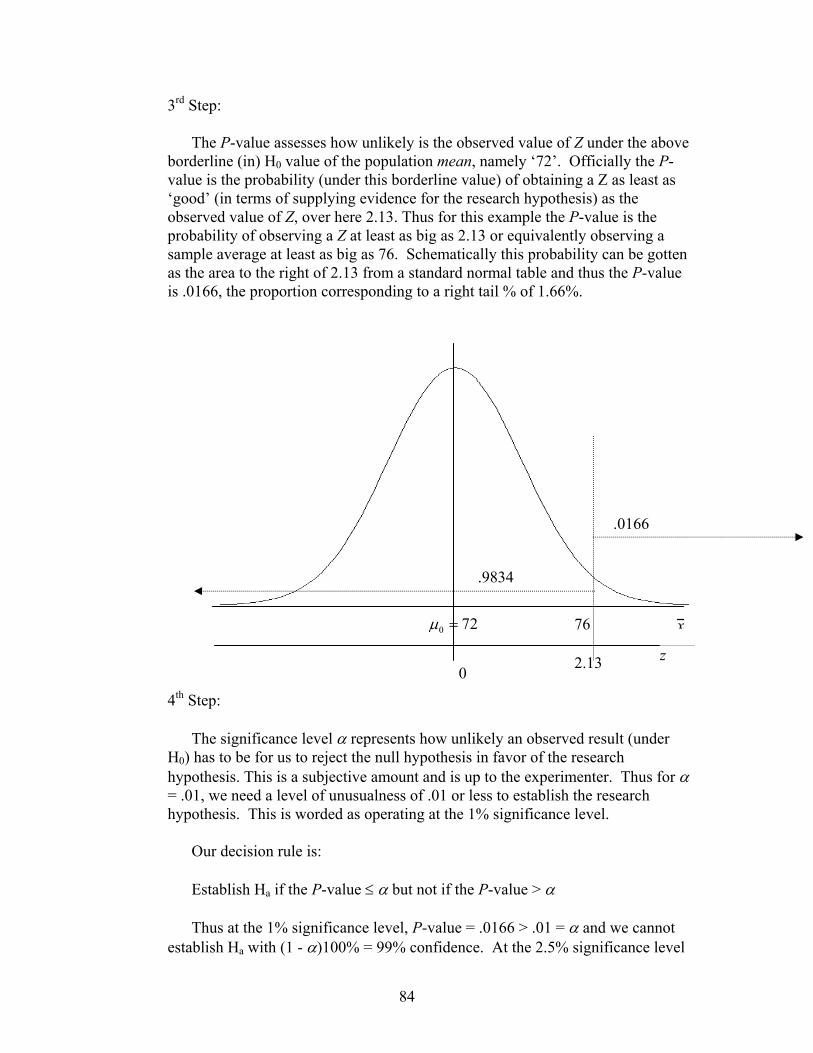
84

3rd Step:

The P-value assesses how unlikely is the observed value of Z under the above borderline (in) H0 value of the population mean, namely ‘72’. Officially the P-value is the probability (under this borderline value) of obtaining a Z as least as ‘good’ (in terms of supplying evidence for the research hypothesis) as the observed value of Z, over here 2.13. Thus for this example the P-value is the probability of observing a Z at least as big as 2.13 or equivalently observing a sample average at least as big as 76. Schematically this probability can be gotten as the area to the right of 2.13 from a standard normal table and thus the P-value is .0166, the proportion corresponding to a right tail % of 1.66%.

4th Step:

The significance level α represents how unlikely an observed result (under H0) has to be for us to reject the null hypothesis in favor of the research hypothesis. This is a subjective amount and is up to the experimenter. Thus for α = .01, we need a level of unusualness of .01 or less to establish the research hypothesis. This is worded as operating at the 1% significance level.

Our decision rule is: Establish Ha if the P-value ≤ α but not if the P-value > α Thus at the 1% significance level, P-value = .0166 > .01 = α and we cannot

establish Ha with (1 - α)100% = 99% confidence. At the 2.5% significance level

μ0 = 72 x

z

76

0 2.13

.9834

.0166

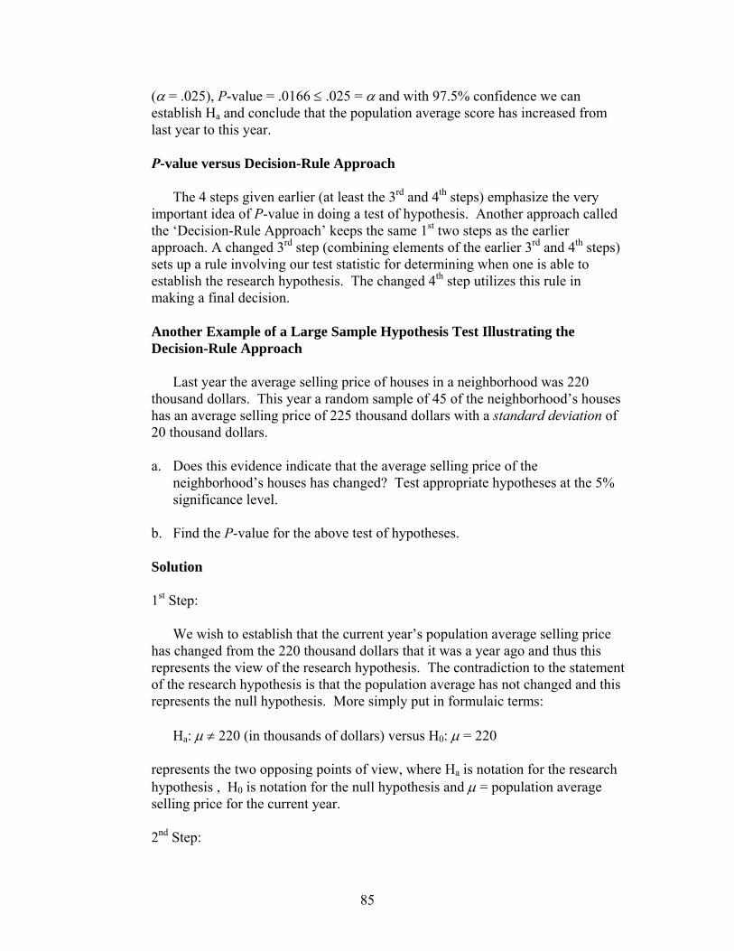
85

(α = .025), P-value = .0166 ≤ .025 = α and with 97.5% confidence we can establish Ha and conclude that the population average score has increased from last year to this year.

P-value versus Decision-Rule Approach

The 4 steps given earlier (at least the 3rd and 4th steps) emphasize the very important idea of P-value in doing a test of hypothesis. Another approach called the ‘Decision-Rule Approach’ keeps the same 1st two steps as the earlier approach. A changed 3rd step (combining elements of the earlier 3rd and 4th steps) sets up a rule involving our test statistic for determining when one is able to establish the research hypothesis. The changed 4th step utilizes this rule in making a final decision. Another Example of a Large Sample Hypothesis Test Illustrating the Decision-Rule Approach

Last year the average selling price of houses in a neighborhood was 220

thousand dollars. This year a random sample of 45 of the neighborhood’s houses has an average selling price of 225 thousand dollars with a standard deviation of 20 thousand dollars.

a. Does this evidence indicate that the average selling price of the

neighborhood’s houses has changed? Test appropriate hypotheses at the 5% significance level.

b. Find the P-value for the above test of hypotheses.

Solution 1st Step:

We wish to establish that the current year’s population average selling price has changed from the 220 thousand dollars that it was a year ago and thus this represents the view of the research hypothesis. The contradiction to the statement of the research hypothesis is that the population average has not changed and this represents the null hypothesis. More simply put in formulaic terms:

Ha: μ ≠ 220 (in thousands of dollars) versus H0: μ = 220

represents the two opposing points of view, where Ha is notation for the research hypothesis , H0 is notation for the null hypothesis and μ = population average selling price for the current year. 2nd Step:

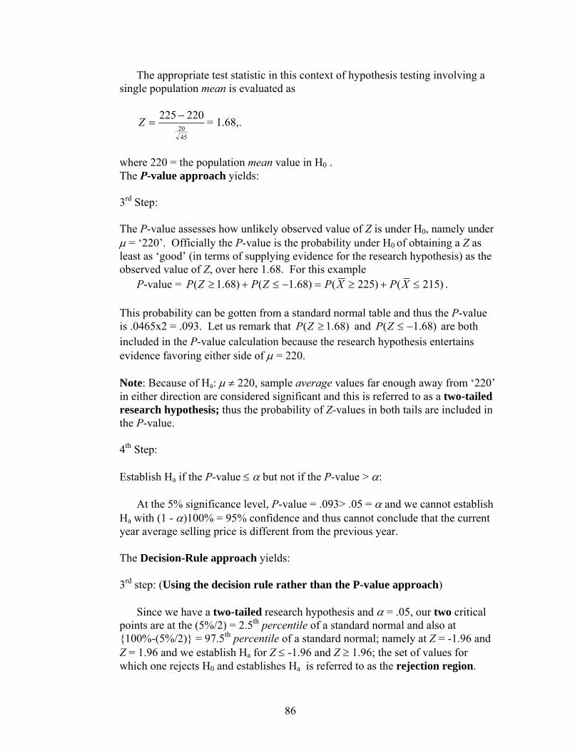
86

The appropriate test statistic in this context of hypothesis testing involving a single population mean is evaluated as

4520

220225 −=Z = 1.68,.

where 220 = the population mean value in H0 . The P-value approach yields: 3rd Step: The P-value assesses how unlikely observed value of Z is under H0, namely under μ = ‘220’. Officially the P-value is the probability under H0 of obtaining a Z as least as ‘good’ (in terms of supplying evidence for the research hypothesis) as the observed value of Z, over here 1.68. For this example P-value = )215()225()68.1()68.1( ≤+≥=−≤+≥ XPXPZPZP . This probability can be gotten from a standard normal table and thus the P-value is .0465x2 = .093. Let us remark that )68.1( ≥ZP and )68.1( −≤ZP are both included in the P-value calculation because the research hypothesis entertains evidence favoring either side of μ = 220.

Note: Because of Ha: μ ≠ 220, sample average values far enough away from ‘220’ in either direction are considered significant and this is referred to as a two-tailed research hypothesis; thus the probability of Z-values in both tails are included in the P-value. 4th Step: Establish Ha if the P-value ≤ α but not if the P-value > α:

At the 5% significance level, P-value = .093> .05 = α and we cannot establish Ha with (1 - α)100% = 95% confidence and thus cannot conclude that the current year average selling price is different from the previous year. The Decision-Rule approach yields: 3rd step: (Using the decision rule rather than the P-value approach)

Since we have a two-tailed research hypothesis and α = .05, our two critical points are at the (5%/2) = 2.5th percentile of a standard normal and also at {100%-(5%/2)} = 97.5th percentile of a standard normal; namely at Z = -1.96 and Z = 1.96 and we establish Ha for Z ≤ -1.96 and Z ≥ 1.96; the set of values for which one rejects H0 and establishes Ha is referred to as the rejection region.

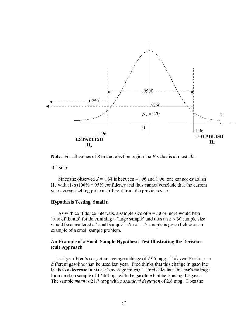
87

Note: For all values of Z in the rejection region the P-value is at most .05.

4th Step:

Since the observed Z = 1.68 is between –1.96 and 1.96, one cannot establish Ha with (1-α)100% = 95% confidence and thus cannot conclude that the current year average selling price is different from the previous year.

Hypothesis Testing, Small n

As with confidence intervals, a sample size of n = 30 or more would be a ‘rule of thumb’ for determining a ‘large sample’ and thus an n < 30 sample size would be considered a ‘small sample’. An n = 17 sample is given below as an example of a small sample problem.

An Example of a Small Sample Hypothesis Test Illustrating the Decision-Rule Approach

Last year Fred’s car got an average mileage of 23.5 mpg. This year Fred uses a different gasoline than he used last year. Fred thinks that this change in gasoline leads to a decrease in his car’s average mileage. Fred calculates his car’s mileage for a random sample of 17 fill-ups with the gasoline that he is using this year. The sample mean is 21.7 mpg with a standard deviation of 2.8 mpg. Does the

μ0 = 220 xz

0 -1.96ESTABLISH Ha

1.96 ESTABLISH Ha

.9750 .0250

.9500

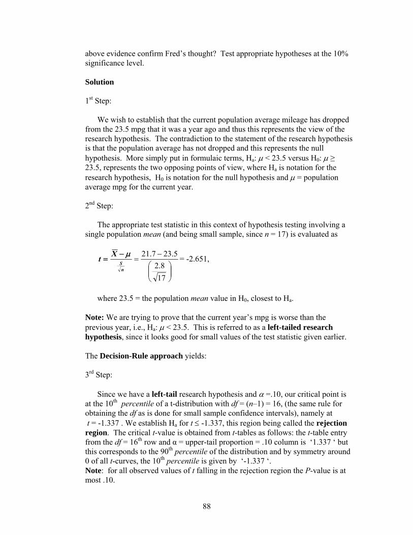
88

above evidence confirm Fred’s thought? Test appropriate hypotheses at the 10% significance level.

Solution 1st Step:

We wish to establish that the current population average mileage has dropped from the 23.5 mpg that it was a year ago and thus this represents the view of the research hypothesis. The contradiction to the statement of the research hypothesis is that the population average has not dropped and this represents the null hypothesis. More simply put in formulaic terms, Ha: μ < 23.5 versus H0: μ ≥ 23.5, represents the two opposing points of view, where Ha is notation for the research hypothesis, H0 is notation for the null hypothesis and μ = population average mpg for the current year. 2nd Step:

The appropriate test statistic in this context of hypothesis testing involving a single population mean (and being small sample, since n = 17) is evaluated as

nS

Xt μ−=

⎟⎟⎠

⎞⎜⎜⎝

⎛−

=

178.2

5.237.21 = -2.651,

where 23.5 = the population mean value in H0, closest to Ha.

Note: We are trying to prove that the current year’s mpg is worse than the previous year, i.e., Ha: μ < 23.5. This is referred to as a left-tailed research hypothesis, since it looks good for small values of the test statistic given earlier.

The Decision-Rule approach yields: 3rd Step:

Since we have a left-tail research hypothesis and α =.10, our critical point is at the 10th percentile of a t-distribution with df = (n–1) = 16, (the same rule for obtaining the df as is done for small sample confidence intervals), namely at t = -1.337 . We establish Ha for t ≤ -1.337, this region being called the rejection region. The critical t-value is obtained from t-tables as follows: the t-table entry from the df = 16th row and α = upper-tail proportion = .10 column is ‘1.337 ‘ but this corresponds to the 90th percentile of the distribution and by symmetry around 0 of all t-curves, the 10th percentile is given by ‘-1.337 ‘. Note: for all observed values of t falling in the rejection region the P-value is at most .10.

89

4th Step:

Since the observed t = -2.651 is at most –1.337, one can establish Ha with at least (1 - α)100% = 90% confidence and thus can conclude that the current year average mpg is less than the previous year’s.

Another Example of a Small Sample Hypothesis Test Last year Sally belonged to an HMO that had a population average rating of 62 (on a scale from 0-100, with ‘100’ being best); this was based on records accumulated about the HMO over a long period of time. This year Sally switched to a new HMO. To assess the population mean rating of the new HMO and to see if it is different than the old HMO, 20 members of this new HMO are polled and they give it an average rating of 65 with a standard deviation of 10. At the 5% level of significance is one of the HMO’s better rated than the other? Solution 1st Step:

We wish to establish that the population average rating for the new HMO is different from the ‘62’ rating of the previous HMO and thus this represents the view of the research hypothesis. The contradiction to the statement of the research hypothesis is that the population average rating is not different and this represents the null hypothesis. More simply put in formulaic terms,

Ha: μ ≠ 62 versus H0: μ = 62,

represents the two opposing points of view, where Ha is notation for the research hypothesis, H0 is notation for the null hypothesis and μ = population average rating for the new HMO. 2nd Step:

The appropriate test statistic in this context of hypothesis testing involving a

single population mean is evaluated as 20

10

6265 −=t = 1.342, where 62 is the

population mean value in H0 .

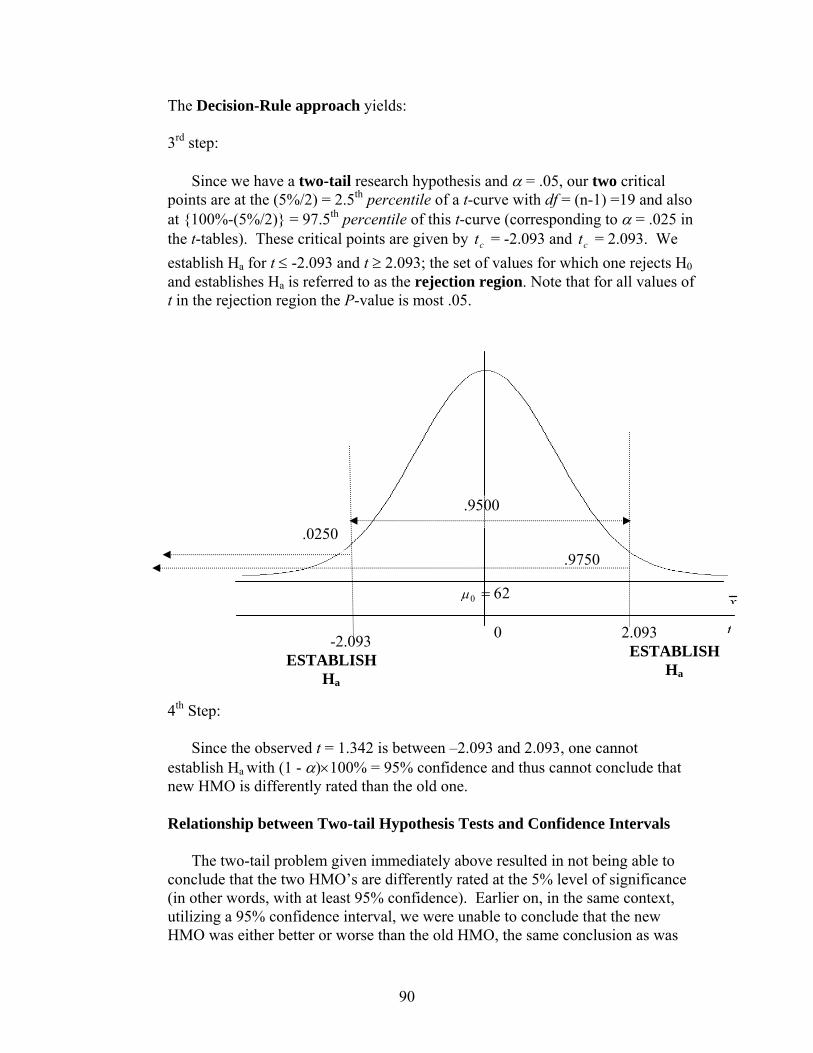
90

The Decision-Rule approach yields: 3rd step:

Since we have a two-tail research hypothesis and α = .05, our two critical points are at the (5%/2) = 2.5th percentile of a t-curve with df = (n-1) =19 and also at {100%-(5%/2)} = 97.5th percentile of this t-curve (corresponding to α = .025 in the t-tables). These critical points are given by ct = -2.093 and ct = 2.093. We establish Ha for t ≤ -2.093 and t ≥ 2.093; the set of values for which one rejects H0 and establishes Ha is referred to as the rejection region. Note that for all values of t in the rejection region the P-value is most .05.

4th Step:

Since the observed t = 1.342 is between –2.093 and 2.093, one cannot establish Ha with (1 - α)×100% = 95% confidence and thus cannot conclude that new HMO is differently rated than the old one. Relationship between Two-tail Hypothesis Tests and Confidence Intervals

The two-tail problem given immediately above resulted in not being able to conclude that the two HMO’s are differently rated at the 5% level of significance (in other words, with at least 95% confidence). Earlier on, in the same context, utilizing a 95% confidence interval, we were unable to conclude that the new HMO was either better or worse than the old HMO, the same conclusion as was

0μ = 62 x

t

0 -2.093 ESTABLISH Ha

2.093 ESTABLISH Ha

.9750 .0250

.9500

91

gotten by the two-tail hypothesis testing approach. These two approaches always give the same conclusion that 1) we can establish what we set out to do or 2) we cannot.

One Sample Mean−Hypothesis Testing Problems LARGE SAMPLE HT = 'hypothesis test' PROBLEMS Chapter 9, pages 77-82 1. An old well-known HMO-A has a known population mean of 50. We investigate a

new HMO, HMO-B, and our desire is to conclude that it is better rated in the population than the old HMO. We sample 49 individuals with the new HMO and obtain a sample average rating of X = 60, with a sample standard deviation of s =30. Can we conclude that HMO-B is better rated? Work at both α = .02 and α = .001.

2. A certain powerful anti-depressant has side-effects so daily dosages must be minimized. However, one patient may need 200 mg per day to relieve depression while another patient may need only 100 mg per day to have the same effect. Researchers are concerned about a report in a journal that the average minimum effective dosage of the drug nationwide is at least 149.5 mg per day. They collect data in order to refute what they feel is a misleading report in this journal. They randomly sample 400 patients nationwide and obtain an average minimum effective dosage of 142.6 mg/day with a sample standard deviation of 48.2. Have these researchers been able to refute the report in the journal at the α = .001 level? Please answer this question by stating the null and research hypothesis, by evaluating the appropriate test statistic, by calculating the P-value and then comparing it to the given α value in making your decision.

3. Last year, the average December residential heating bill was $93.41. A random

sample of 41 residential heating bills has a mean amount of $96.52 with a standard deviation of $10.34.

a. Does this information indicate that the average residential heating bill has

changed? Test appropriate hypotheses at the 10% significance level. b. Find the P-value for the above test of hypotheses.

92

4. The average daily sales in the men’s clothing department for a department store chain

is 7.1 thousand dollars. A random sample of 64 men’s clothing departments was taken on the day after Thanksgiving. The sample mean sales on that day was 7.8 thousand dollars with a standard deviation of 2.3 thousand dollars. Does this evidence suggest that the average daily sales in the men’s department for the department store chain is higher on the day after Thanksgiving than it is otherwise? Test appropriate hypotheses at the 1% significance level.

5. The average amount of grams of fat in a certain product is advertised as being no more

than 4. We suspect that this is wrong and we collect data for the purpose of disproving this claim. We randomly sample 64 units of this product and obtain an X -Value of 4.5 with an s-value of 1.6. Can we conclude that the claim has been disproven?

6. To prove that the population mean amount of time that it takes to perform a certain job

is less than 70 minutes. We sample 100 individuals and obtain an X of 67.3 with an s of 15. Can we establish the above?

7. Can we prove that a 20-ounce catsup bottle contains something other than the labeled

amount? (Test at α = .05). DATA: n=36, X =19.7 ounces, s = 0.6 ounces.

93

SMALL SAMPLE HT = 'hypothesis test' PROBLEMS Chapter 9, pages 82-86

8. The average number of years of post secondary education of employees in an industry

is 1.5. A company claims that this average is higher for its employees. A random sample of 16 of its employees has an average of 2.1 years of post secondary education with a standard deviation of .6 years. Is this average higher for the company’s employees? Test appropriate hypotheses at the 5% significance level.

9. Fred frequently drives his car to Sacramento. His auto club suggests that it takes 90 minutes to drive to there. A random sample of 10 of Fred’s trips to Sacramento took an average of 85 minutes with a standard deviation of 8 minutes. Does this evidence indicate that Fred’s average driving time to Sacramento differs from the 90 minutes suggested by his auto club? Test appropriate hypotheses at the 5% significance level.

94

C. Using Excel for One Sample Inference

For summary data, the CONFIDENCE function will return the margin of error for a confidence interval. Using the example from IX-A, a random sample of 41 residential heating bills has a mean amount of $96.52 with a standard deviation of $10.34. Find a 95% confidence interval for the mean of all residential heating bills:

Highlight any cell and click the fx button, Statistical Functions and scroll down and click the function CONFIDENCE.

Set “Alpha” equal to 0.05, the significance level.

Set “Standard_Dev” equal to 10.34, the sample standard deviation. Set “Size” equal to 41, the sample size

The function returns the Margin of Error of $3.17, which can be added to and subtracted from the sample mean of $95.62 to obtain a 95% confidence interval for μ of ($93.35, $99.69).

One population hypothesis testing for the mean is not built into Excel, but p-values can be calculated using TDIST function. Let us recall the example from IX-B: Last year Sally belonged to an HMO that had a population average rating of 62 (on a scale from 0-100, with ‘100’ being best); this was based on records accumulated about the HMO over a long period of time. This year Sally switched to a new HMO. To assess the population mean rating of the new HMO and to see if it is different than the old HMO, 20 members of this new HMO are polled and they give it an average rating of 65 with a standard deviation of 10. At the 5% level of significance is one of the HMO’s better rated than the other?

1) First, calculate the t statistic using the formula n

S

Xt μ−= , obtaining 1.342.

2) Highlight any cell and click the fx button, Statistical Functions and scroll down and click the TDIST function. Set “X” equal to 1.342, the value of t. If this number is negative, you must enter the absolute value of t and switch to the upper tail in a one-tailed test. Set “Deg_freedom” equal to 19, one less than the sample size. Set “Tails” equal to 2, since this is a two-tailed test.

The function returns the p-value of .1954, which is greater than α = .05 and leads

to the decision of Fail to Reject Ho.

95

X. One Sample Inference: Qualitative Data

Confidence Intervals We are assuming in this context that we are dealing with binomial (success-failure) data. The population mean no longer has a meaning since the data is non-numerical. We are now interested in inference on π = population proportion, referred to as the ‘probability of success’ earlier on in the discussion of the binomial in the non-inference context. For example in a population of motorists, π = proportion of motorists with cell telephones in their cars; in the inference context, we assume that π is unknown. p = sample proportion with cell phones is the statistic from the data that is used to estimate π (replacing X that is used with the population mean). For example if 200 motorists were sampled from the population and 25 had cell phones then the sample proportion is given by p = (# with phones)/(size of the sample) = (25/200) = 0.125.

The formula for the limits of a large sample confidence interval for π

(abbreviated as CI), is given by

nppzp c

)1( −±=π ,

where n = sample size and where cz > 0 is chosen so that the % under a standard normal curve between - cz and + cz is equal to the specified confidence %, i.e., so that the middle % under a standard normal curve is equal to the confidence %.

Determination of the sample size n:

One can also set the confidence level at some % and set the margin of error E at some desired amount and use the equation

(1 )

cp pE z

n−

=

to solve for n resulting in

)1(2

ppEz

n c −⎟⎠

⎞⎜⎝

⎛= ;

if one has no knowledge of p , use p = 0.5, since the quantity )1( pp − is maximized when p = 0.5.

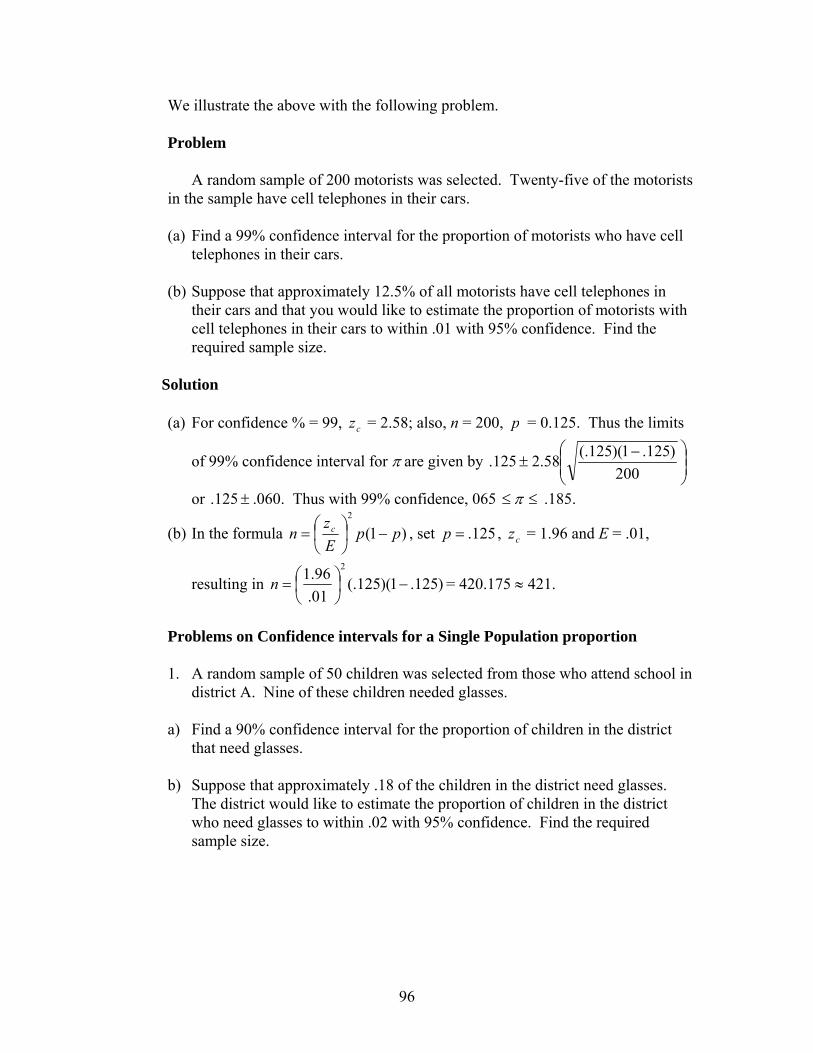
96

We illustrate the above with the following problem. Problem

A random sample of 200 motorists was selected. Twenty-five of the motorists in the sample have cell telephones in their cars.

(a) Find a 99% confidence interval for the proportion of motorists who have cell

telephones in their cars.

(b) Suppose that approximately 12.5% of all motorists have cell telephones in their cars and that you would like to estimate the proportion of motorists with cell telephones in their cars to within .01 with 95% confidence. Find the required sample size.

Solution (a) For confidence % = 99, cz = 2.58; also, n = 200, p = 0.125. Thus the limits

of 99% confidence interval for π are given by ⎟⎟⎠

⎞⎜⎜⎝

⎛ −±

200)125.1)(125(.58.2125.

or ±125. .060. Thus with 99% confidence, 065 ≤≤ π .185.

(b) In the formula )1(2

ppEz

n c −⎟⎠⎞

⎜⎝⎛= , set 125.=p , cz = 1.96 and E = .01,

resulting in )125.1)(125(.01.96.1 2

−⎟⎠⎞

⎜⎝⎛=n = 420.175 ≈ 421.

Problems on Confidence intervals for a Single Population proportion 1. A random sample of 50 children was selected from those who attend school in

district A. Nine of these children needed glasses. a) Find a 90% confidence interval for the proportion of children in the district

that need glasses. b) Suppose that approximately .18 of the children in the district need glasses.

The district would like to estimate the proportion of children in the district who need glasses to within .02 with 95% confidence. Find the required sample size.

97

2. A random sample of 200 of a town’s residents is taken. There are 80 renters in the sample. Find a 95% confidence interval for the proportion of the town’s residents that are renters.

3. A random sample of 1000 items is selected from those produced by a factory.

50 of these items are defective. Obtain a 90% confidence interval for the proportion of defective items among those produced by the factory.

4. We are interested in the population proportion of all traffic accidents, where

eating or drinking was a major contributor to the accident. Our desire is to operate at 99.8% confidence, with a margin of error of .05.

(a) Obtain the required total sample size. (b) Suppose that we sampled the number of traffic accidents prescribed in (a),

and it was found that in 180 of those accidents, eating or drinking was a major contributor to the accident. Obtain a 99.8% CI for the above population proportion.

(c) Obtain the margin of error for the CI of (b). Explain why it is smaller than the desired amount of .05.

98

Hypothesis Testing

We are assuming in this context that we are dealing with binomial (success-failure) data. The population mean no longer has a meaning since the data is non-numerical. We are now interested in inference on π = population proportion, referred to as the ‘probability of success’ earlier on in the discussion of the binomial in the non-inference context.

For example in a population of children, π = proportion of children in the

population needing glasses; in the inference context, we assume that π is unknown. p = sample proportion needing glasses is the statistic from the data that is used to estimate π (replacing X that is used with the population mean). For example if 50 children were sampled from the population and 9 needed glasses then the sample proportion is given by p = # needing glasses/size of the sample = 9/50 = 0.18. We illustrate inference procedures involving π and p with some examples given below.

Example of Hypothesis Test

A random sample of 50 children was selected from those who attend school in District A. Nine of these children needed glasses. It is believed that less than 25% of the children in the district need glasses. Does the above information confirm this belief? Test appropriate hypotheses at the 10% significance level.

Solution 1st Step:

We wish to establish that the population proportion is below 0.25 and this represents the view of the research hypothesis. The contradiction to the statement of the research hypothesis is that the population proportion is at least 0.25 and this represents the null hypothesis. More simply put in formulaic terms,

Ha: π < 0.25 versus H0: π ≥ 0.25

represents the two opposing points of view, where Ha is notation for the research hypothesis and H0 is notation for the null hypothesis and π = population proportion needing glasses.

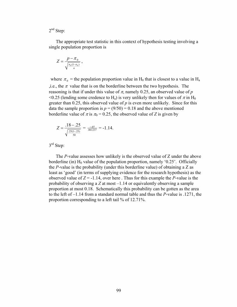
99

2nd Step:

The appropriate test statistic in this context of hypothesis testing involving a single population proportion is

n

pZ

)1(

0

00 ππ

π−

−= ,

where 0π = the population proportion value in H0 that is closest to a value in Ha

,i.e., the π value that is on the borderline between the two hypothesis. The reasoning is that if under this value of π, namely 0.25, an observed value of p <0.25 (lending some credence to Ha) is very unlikely then for values of π in H0 greater than 0.25, this observed value of p is even more unlikely. Since for this data the sample proportion is p = (9/50) = 0.18 and the above mentioned borderline value of π is π0 = 0.25, the observed value of Z is given by

50)25.1(25.

25.18.−

−=Z = 061237.

07.− = -1.14.

3rd Step:

The P-value assesses how unlikely is the observed value of Z under the above borderline (in) H0 value of the population proportion, namely ‘0.25’. Officially the P-value is the probability (under this borderline value) of obtaining a Z as least as ‘good’ (in terms of supplying evidence for the research hypothesis) as the observed value of Z = -1.14, over here . Thus for this example the P-value is the probability of observing a Z at most –1.14 or equivalently observing a sample proportion at most 0.18. Schematically this probability can be gotten as the area to the left of –1.14 from a standard normal table and thus the P-value is .1271, the proportion corresponding to a left tail % of 12.71%.

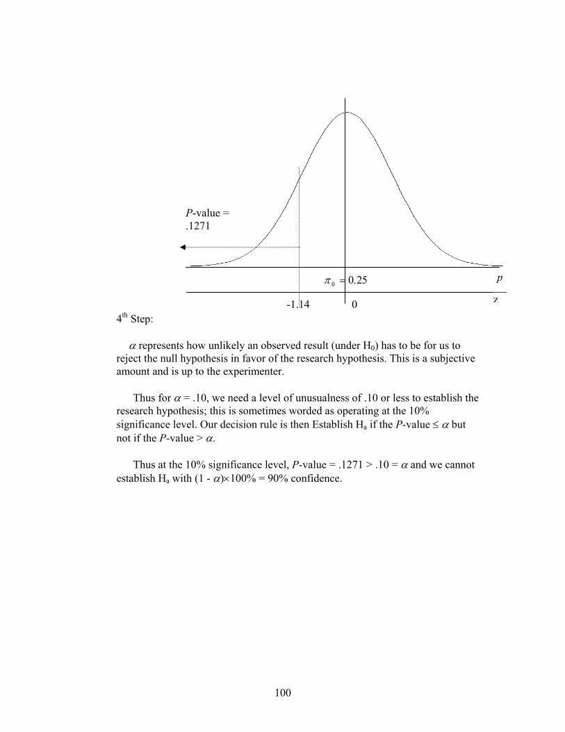
100

4th Step:

α represents how unlikely an observed result (under H0) has to be for us to reject the null hypothesis in favor of the research hypothesis. This is a subjective amount and is up to the experimenter.

Thus for α = .10, we need a level of unusualness of .10 or less to establish the

research hypothesis; this is sometimes worded as operating at the 10% significance level. Our decision rule is then Establish Ha if the P-value ≤ α but not if the P-value > α.

Thus at the 10% significance level, P-value = .1271 > .10 = α and we cannot

establish Ha with (1 - α)×100% = 90% confidence.

0π = 0.25 p

z

0 -1.14

P-value = .1271

101

Problems on Hypothesis Testing for a Single Population proportion 1. A random sample of 200 motorists was selected. Twenty-five of the

motorists in the sample have cell telephones in their cars. An insurance company official claims that more than 10% of motorists have cell telephones in their cars. Does the above evidence support this claim? Test appropriate hypotheses at the 10% significance level.

2. A random sample of 200 of a town’s residents is taken. There are 80 renters

in the sample. Does this evidence indicate that it is not the case that 30% of the town’s residents are renters? Work the test at the 5% significance level.

3. We wish to establish that less than 12% of traffic accidents have adjusting the radio, cassette, or CD as a contributor to the accident. We randomly sample the records for 500 accidents and find that in 50 of those accidents, adjusting the radio, etceteras, was a contributor to the accident. Can it be concluded at

the 1% significance level (α = .01) that less than 12% of all traffic accidents have adjusting the radio, cassette, or CD as a contributor to the accident?

102

XI. Two sample Inference: Quantitative Data A. Large & Small Samples

For the earlier one sample quantitative problems, we sample from just one group and have only one unknown population mean to worry about. For example suppose a longtime HMO had a known population mean rating of 60 (on a scale from 0-100). We sample the customers of a new HMO in order to make an inference about μ, the unknown population mean for the new HMO. The nature of the research hypothesis depends on what we are trying to establish. If 1) we are trying to prove that the new HMO is better rated (than the old) in the

population then Ha: μ > 60 (vs. H0: μ ≤ 60). This is referred to as a right-tail research hypothesis, since it looks good for large values of the test statistic given earlier.

2) we are trying to prove that the new HMO is worse rated in the population then Ha: μ < 60 (vs. H0: μ ≥ 60) . This is referred to as a left-tail research hypothesis, since it looks good for small values of the test statistic given earlier.

3) we are trying to prove that the new HMO is not equally rated (i.e., it is of interest to us to show that it is either more highly rated or less highly rated in the population) then Ha: μ ≠ 60 (vs. H0: μ = 60) . This is referred to as a two-tail research hypothesis, since it looks good for either small or large values of the test statistic given earlier.

Suppose, on the other hand, we were comparing two HMO’s and both population

means were unknown, say where μi = population mean for the ith HMO, we then need two samples, one from each group. We are then in a two-sample context.

In an analogous manner as described above there are 3 possible research

hypothesis, to show that the 1st HMO is better, Ha: μ1 > μ2 (vs. H0: μ1 ≤ μ2 ), or to show that the 2nd HMO is better, , Ha: μ1 < μ2 , or to show that the two HMO’s are not equally rated, Ha: μ1 ≠ μ2 , i.e., trying to show that one of the two HMO’s is better than the other without specifying which of the two HMO’s is the better one. We give an example of this two-sample problem below.

Example of Hypothesis Test: Large Samples

We wish to compare two HMO’s in terms of how they are rated (on a scale from 0-

100) by their customers. A random sample of 100 customers of HMO-A are selected and asked to rate this first HMO. Also a random sample of 100 customers from HMO-B is asked to rate this second HMO. The results are that for the first HMO the average rating is 80 with a sample standard deviation of 7 and for the second, the average was 76 with a standard deviation of 10. Can it be concluded that on a population wide basis (as opposed to simply a sample result), one of the two HMO’s is rated higher than the other HMO? Test appropriate hypotheses at the 2.5% significance level.

103

Solution

1st Step:

We wish to establish that the population mean rating of the 1st HMO is different from

the population mean of the 2nd HMO and this represents the view of the research hypothesis, i.e., that the two HMO’s are not equally rated in the population. The contradiction to the statement of the research hypothesis is that the two population means are the same for both HMO’s and this represents the null hypothesis. More simply put in formulaic terms,

Ha: μ1 ≠ μ2 versus H0: μ1 = μ2,

represents the two opposing points of view, where Ha is notation for the research hypothesis and H0 is notation for the null hypothesis and μi = population mean for the ith HMO.

2nd Step:

The appropriate test statistic in this context of hypothesis testing involving a

comparison of two population means is

2

22

1

21

21

ns

ns

XXZ

+

−= .

For this data, the observed value of Z is given by

10010

1007

768022

+

−=Z = (4/1.22066) = 3.28.

3rd Step:

The P-value assesses how unlikely is the observed value of Z under the above H0.

Officially the P-value is the probability (under the assumption that the HMO’s are equally rated in the population) of obtaining a Z as least as ‘good’ (in terms of supplying evidence for the research hypothesis) as the observed value of Z = 3.28.

Thus, for this example, the P-value is the estimated probability of observing a Z of at

least 3.28 (representing results at least as outstanding as the observed result in the direction favoring HMO-A as being better rated). This probability needs to be added to the estimated probability of observing a Z-value of at most –3.28, representing results at least as good as the observed result but in the opposite direction.

104

Schematically the P-value probability can be gotten as the area to the left of –3.28 + the area to the right of +3.28 from a standard normal table and thus the P-value is .0010, the proportion corresponding to a (left tail + right tail %) of .05%+ .05% =.10%. 4th Step:

α represents how unlikely an observed result (under H0) has to be for us to reject the

null hypothesis in favor of the research hypothesis. This is a subjective amount and is up to the experimenter. Thus for α = .025, we need a level of unusualness of .025 or less to establish the research hypothesis; this is sometimes worded as operating at the 2.5% significance level. Our decision rule is then Establish Ha if the P-value ≤ α but not if the P-value > α’; thus at the 2.5% significance level, P-value = .0010 ≤ .025 = α and we can establish Ha with at least (1 - α)×100% = 97.5% confidence.

Another Example of a Two-Sample Hypothesis Test: Large Samples

We wish to show that reading Jerry Lucas’s memory book helps improve someone’s

memory. A group of 150 people who have not read the book are randomly selected and given a memory test (scored on a scale from 0-50) and their average score is 25 with a standard deviation of 8. A second group of 50 individuals are randomly selected, asked to read the memory book and then tested. The average score for this 2nd group is 35 with a standard deviation of 12. Can it be concluded that reading the memory book helps improve someone’s memory. Operate at the 1% significance level.

μ1 − μ2 = 0 21 xx −

z

0 -3.28 3.28

.9995.0005

.9990

.0005

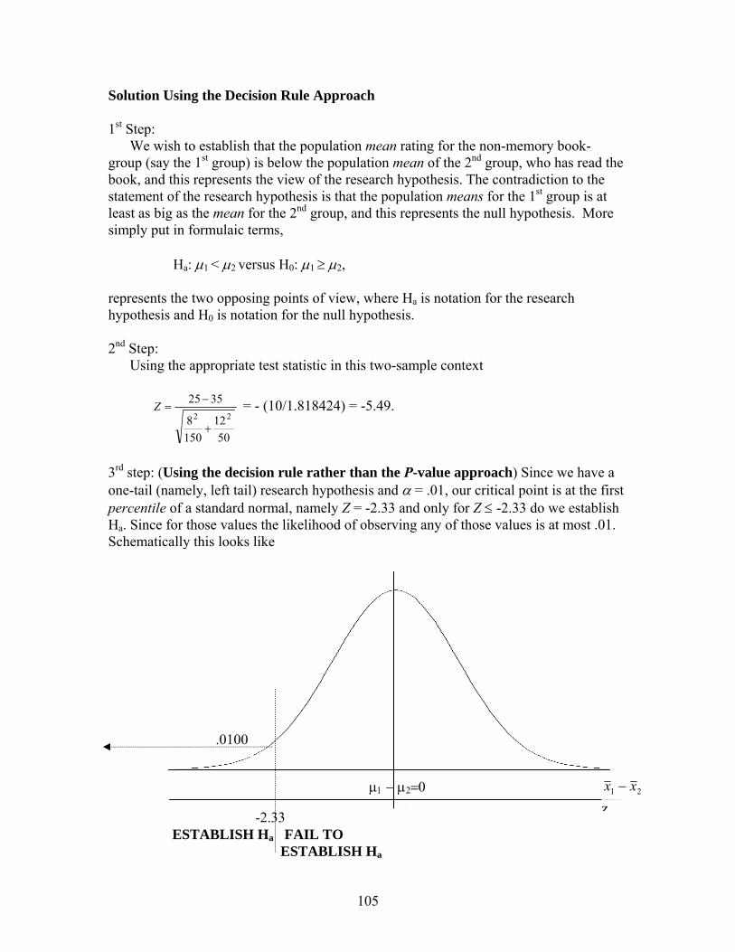
105

Solution Using the Decision Rule Approach 1st Step:

We wish to establish that the population mean rating for the non-memory book-group (say the 1st group) is below the population mean of the 2nd group, who has read the book, and this represents the view of the research hypothesis. The contradiction to the statement of the research hypothesis is that the population means for the 1st group is at least as big as the mean for the 2nd group, and this represents the null hypothesis. More simply put in formulaic terms,

Ha: μ1 < μ2 versus H0: μ1 ≥ μ2,

represents the two opposing points of view, where Ha is notation for the research hypothesis and H0 is notation for the null hypothesis. 2nd Step: Using the appropriate test statistic in this two-sample context

5012

1508

352522

+

−=Z = - (10/1.818424) = -5.49.

3rd step: (Using the decision rule rather than the P-value approach) Since we have a one-tail (namely, left tail) research hypothesis and α = .01, our critical point is at the first percentile of a standard normal, namely Z = -2.33 and only for Z ≤ -2.33 do we establish Ha. Since for those values the likelihood of observing any of those values is at most .01. Schematically this looks like

μ1 − μ2=0 21 xx −

z0 -2.33 ESTABLISH Ha FAIL TO ESTABLISH Ha

.0100

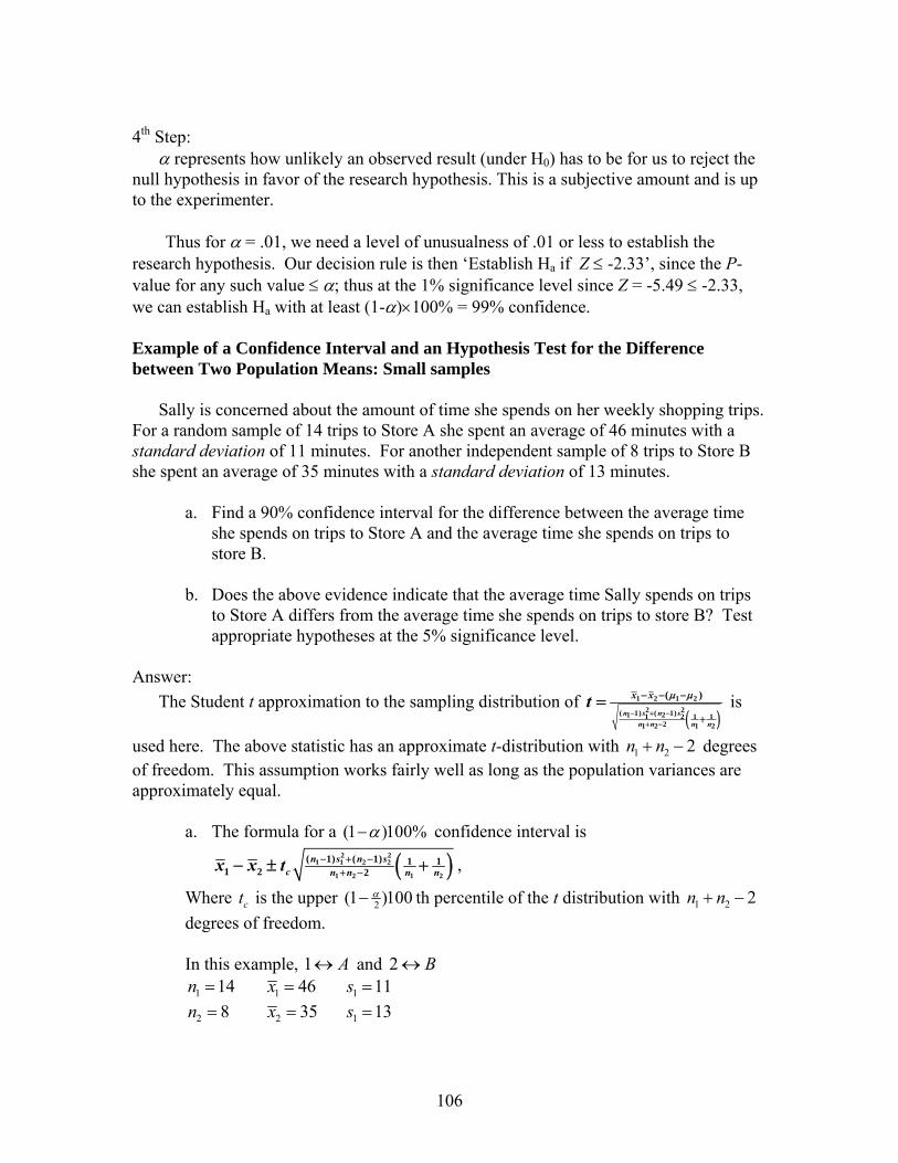
106

4th Step:

α represents how unlikely an observed result (under H0) has to be for us to reject the null hypothesis in favor of the research hypothesis. This is a subjective amount and is up to the experimenter.

Thus for α = .01, we need a level of unusualness of .01 or less to establish the research hypothesis. Our decision rule is then ‘Establish Ha if Z ≤ -2.33’, since the P-value for any such value ≤ α; thus at the 1% significance level since Z = -5.49 ≤ -2.33, we can establish Ha with at least (1-α)×100% = 99% confidence.

Example of a Confidence Interval and an Hypothesis Test for the Difference between Two Population Means: Small samples Sally is concerned about the amount of time she spends on her weekly shopping trips. For a random sample of 14 trips to Store A she spent an average of 46 minutes with a standard deviation of 11 minutes. For another independent sample of 8 trips to Store B she spent an average of 35 minutes with a standard deviation of 13 minutes. a. Find a 90% confidence interval for the difference between the average time

she spends on trips to Store A and the average time she spends on trips to store B.

b. Does the above evidence indicate that the average time Sally spends on trips

to Store A differs from the average time she spends on trips to store B? Test appropriate hypotheses at the 5% significance level.

Answer: The Student t approximation to the sampling distribution of

( )1 2 1 2

2 2( 1) ( 1)1 21 2 1 121 2 1 2

( )

n s n sn n n n

x xt μ μ

− + −+ −

− − −

+= is

used here. The above statistic has an approximate t-distribution with 1 2 2n n+ − degrees of freedom. This assumption works fairly well as long as the population variances are approximately equal.

a. The formula for a (1 )100%α− confidence interval is

( )2 21 1 2 2

1 2 1 2

( 1) ( 1) 1 11 2 2

n s n sc n n n nx x t − + −

+ −− ± + ,

Where ct is the upper 2(1 )100α− th percentile of the t distribution with 1 2 2n n+ − degrees of freedom. In this example, 1 A↔ and 2 B↔

1 14n = 1 46x = 1 11s =

2 8n = 2 35x = 1 13s =

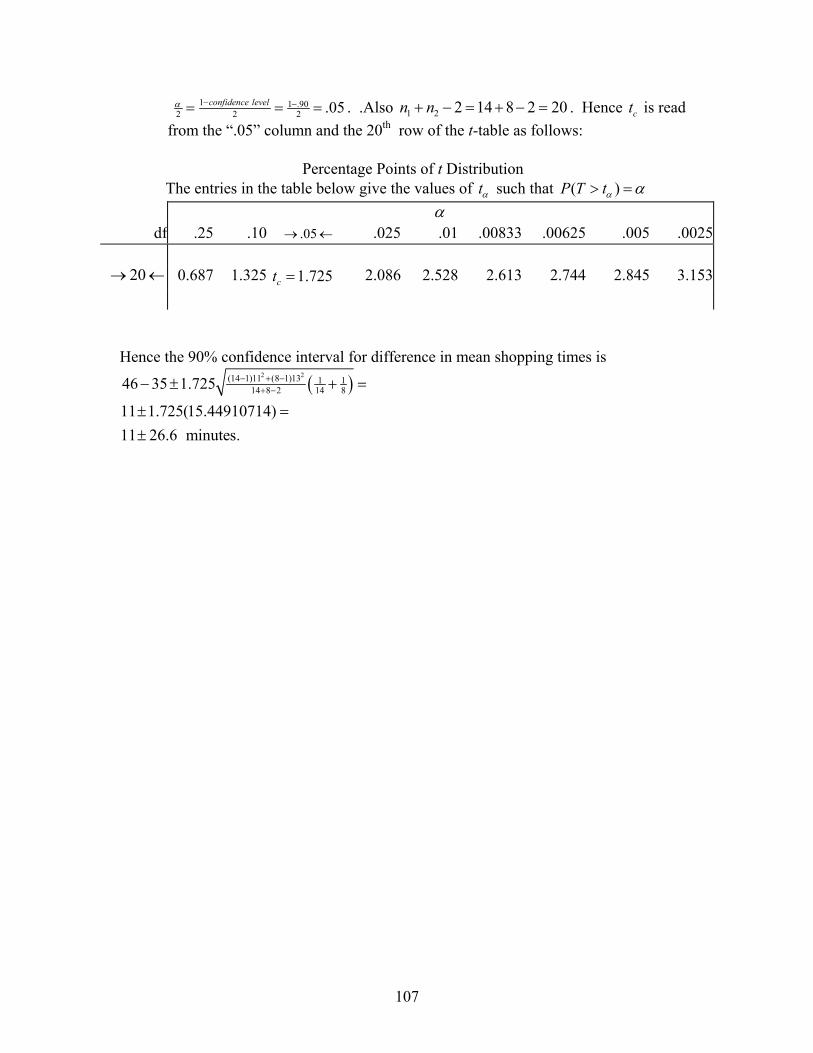
107

1 1 .902 2 2 .05confidence levelα − −= = = . .Also 1 2 2 14 8 2 20n n+ − = + − = . Hence ct is read

from the “.05” column and the 20th row of the t-table as follows:

Percentage Points of t Distribution The entries in the table below give the values of tα such that ( )P T tα α> =

α df .25 .10 .05→ ← .025 .01 .00833 .00625 .005 .0025

20→ ← 0.687 1.325 1.725ct = 2.086 2.528 2.613 2.744 2.845 3.153

Hence the 90% confidence interval for difference in mean shopping times is

( )2 2(14 1)11 (8 1)13 1 114 8 2 14 846 35 1.725

11 1.725(15.44910714)11 26.6 minutes.

− + −+ −− ± + =

± =±

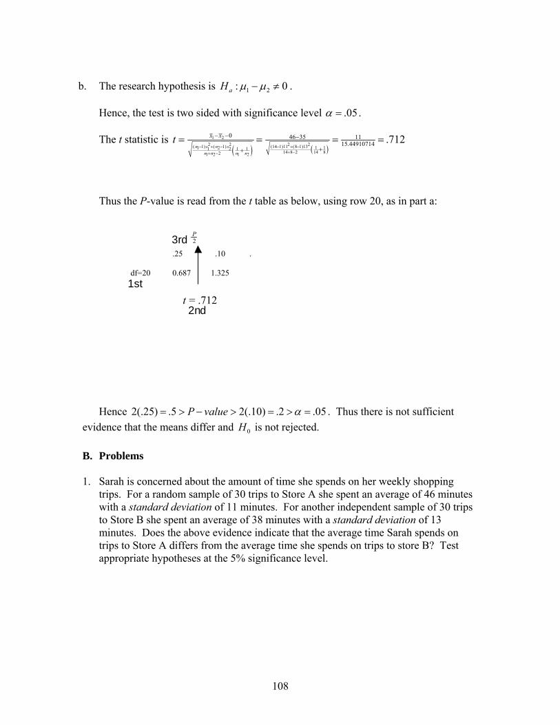
108

b. The research hypothesis is 1 2: 0aH μ μ− ≠ .

Hence, the test is two sided with significance level .05α = .

The t statistic is ( ) ( )

1 22 2 2 2( 1) ( 1) (14 1)11 (8 1)13 1 11 21 2 1 1

14 8 2 14 821 2 1 2

0 46 35 1115.44910714 .712

n s n sn n n n

x xt− + − − + −

+ −+ −

− − −

++= = = =

Thus the P-value is read from the t table as below, using row 20, as in part a:

.25 .10 . df=20 0.687 1.325

t = .712

1st

2nd

3rd 2P

Hence 2(.25) .5 2(.10) .2 .05P value α= > − > = > = . Thus there is not sufficient

evidence that the means differ and 0H is not rejected.

B. Problems

1. Sarah is concerned about the amount of time she spends on her weekly shopping trips. For a random sample of 30 trips to Store A she spent an average of 46 minutes with a standard deviation of 11 minutes. For another independent sample of 30 trips to Store B she spent an average of 38 minutes with a standard deviation of 13 minutes. Does the above evidence indicate that the average time Sarah spends on trips to Store A differs from the average time she spends on trips to store B? Test appropriate hypotheses at the 5% significance level.

109

2. Fred commutes to work on route A or route B. For a random sample of 50 trips using route A, his commuting time averaged 57 minutes with a standard deviation of 15 minutes. For another independent sample of 56 trips on route B, his commuting time averaged 62 minutes with a standard deviation of 20 minutes. Does the above evidence indicate that Fred’s average commuting time is larger when he uses route B than when he uses route A? Test appropriate hypotheses at the 5% significance level.

3. Tom gets consulting calls from customers A and B. For a random sample of 5 calls from customer A, his consulting time averaged 45 minutes with a standard deviation of 10 minutes. For another independent sample of 6 calls from B, his consulting time averaged 62 minutes with a standard deviation of 12 minutes.

a. Find a 90% confidence interval for the difference between Tom’s average consulting time with customer A and that with customer B.

b. Does the above evidence indicate that the Tom’s average consulting time is

larger when he consults with B than when he consults with A? Test appropriate hypotheses at the 5% significance level.

4. Sam and Ted frequently go fishing for salmon. A random sample of 7 of the

salmon that Ted caught has mean weight of 13.2 pounds with a standard

110

deviation of 5 pounds. An independent sample of the salmon that Sam caught has mean weight of 15.4 pounds with a standard deviation of 6 pounds.

a. Find a 95% confidence interval for the difference between the average weight

of the salmon that Ted catches and the average weight of the salmon that Sam catches.

b. Does the above evidence indicate that the average weight of the salmon that

Ted catches differs from the average weight of salmon that Sam catches? Test appropriate hypotheses at the 10% significance level.

5. Harry commutes to work on route A or route B. For a random sample of 5 trips

using route A, his commuting time averaged 45 minutes with a standard deviation of 10 minutes. For another independent sample of 6 trips on route B, his commuting time averaged 62 minutes with a standard deviation of 12 minutes.

a. Find a 99% confidence interval for the difference between Harry’s average

commuting time on route A and that on route B.. b. Does the above evidence indicate that the Harry’s average commuting time

when he uses route B differs from his average commuting time when he uses route A? Test appropriate hypotheses at the 1% significance level.

C. Using Excel for Two Sample Inference

The Data Analysis has a built-in test for the two-population hypothesis test for the mean. Here is an example: Average gas mileage in miles per gallon (MPG) was measured for 8 US Cars and 9 Import Cars:

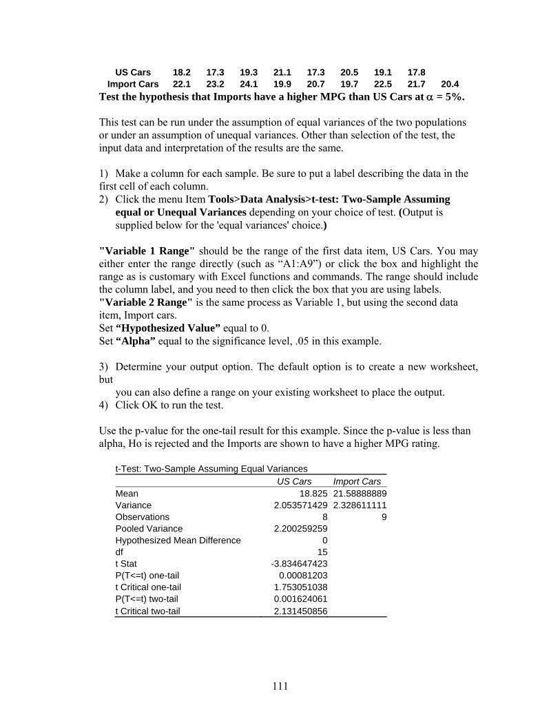
111

US Cars 18.2 17.3 19.3 21.1 17.3 20.5 19.1 17.8 Import Cars 22.1 23.2 24.1 19.9 20.7 19.7 22.5 21.7 20.4

Test the hypothesis that Imports have a higher MPG than US Cars at α = 5%. This test can be run under the assumption of equal variances of the two populations or under an assumption of unequal variances. Other than selection of the test, the input data and interpretation of the results are the same. 1) Make a column for each sample. Be sure to put a label describing the data in the first cell of each column. 2) Click the menu Item Tools>Data Analysis>t-test: Two-Sample Assuming

equal or Unequal Variances depending on your choice of test. (Output is supplied below for the 'equal variances' choice.)

"Variable 1 Range" should be the range of the first data item, US Cars. You may either enter the range directly (such as “A1:A9”) or click the box and highlight the range as is customary with Excel functions and commands. The range should include the column label, and you need to then click the box that you are using labels. "Variable 2 Range" is the same process as Variable 1, but using the second data item, Import cars.

Set “Hypothesized Value” equal to 0. Set “Alpha” equal to the significance level, .05 in this example.

3) Determine your output option. The default option is to create a new worksheet, but

you can also define a range on your existing worksheet to place the output. 4) Click OK to run the test.

Use the p-value for the one-tail result for this example. Since the p-value is less than alpha, Ho is rejected and the Imports are shown to have a higher MPG rating.

t-Test: Two-Sample Assuming Equal Variances US Cars Import Cars

Mean 18.825 21.58888889Variance 2.053571429 2.328611111Observations 8 9Pooled Variance 2.200259259 Hypothesized Mean Difference 0 df 15 t Stat -3.834647423 P(T<=t) one-tail 0.00081203 t Critical one-tail 1.753051038 P(T<=t) two-tail 0.001624061 t Critical two-tail 2.131450856

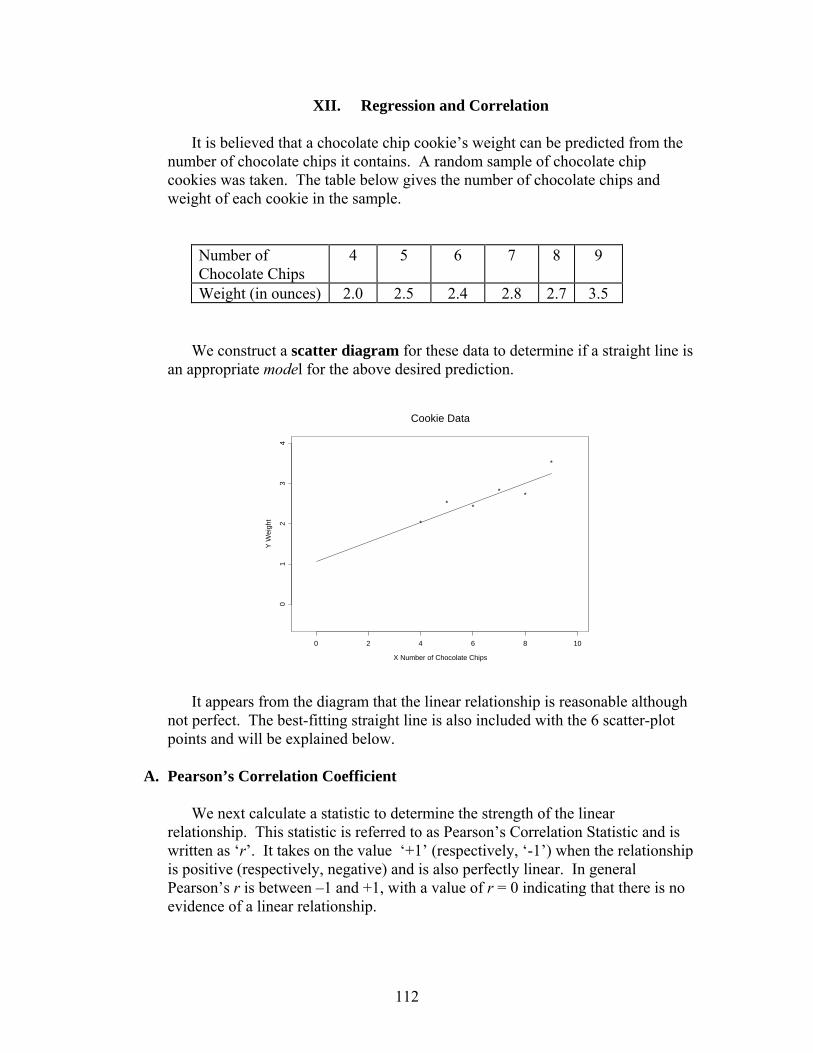
112

XII. Regression and Correlation

It is believed that a chocolate chip cookie’s weight can be predicted from the number of chocolate chips it contains. A random sample of chocolate chip cookies was taken. The table below gives the number of chocolate chips and weight of each cookie in the sample.

Number of Chocolate Chips

4 5 6 7 8 9

Weight (in ounces) 2.0 2.5 2.4 2.8 2.7 3.5

We construct a scatter diagram for these data to determine if a straight line is an appropriate model for the above desired prediction.

It appears from the diagram that the linear relationship is reasonable although

not perfect. The best-fitting straight line is also included with the 6 scatter-plot points and will be explained below.

A. Pearson’s Correlation Coefficient

We next calculate a statistic to determine the strength of the linear

relationship. This statistic is referred to as Pearson’s Correlation Statistic and is written as ‘r’. It takes on the value ‘+1’ (respectively, ‘-1’) when the relationship is positive (respectively, negative) and is also perfectly linear. In general Pearson’s r is between –1 and +1, with a value of r = 0 indicating that there is no evidence of a linear relationship.

*

* *

* *

*

Cookie Data

X Number of Chocolate Chips

Y W

eigh

t

0 2 4 6 8 10

01

23

4

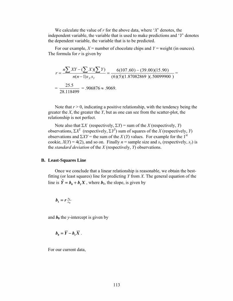
113

We calculate the value of r for the above data, where ‘X’ denotes, the independent variable, the variable that is used to make predictions and ‘Y’ denotes the dependent variable, the variable that is to be predicted.

For our example, X = number of chocolate chips and Y = weight (in ounces). The formula for r is given by

YX ssnnYXXYn

r)1(

))((−

−= ∑ ∑ ∑

)50099900)(.87082869.1)(5)(6()90.15)(00.39()60.107(6 −

= =

= 118499.28

5.25 = .906876 ≈ .9069.

Note that r > 0, indicating a positive relationship, with the tendency being the greater the X, the greater the Y, but as one can see from the scatter-plot, the relationship is not perfect.

Note also that ΣX (respectively, ΣY) = sum of the X (respectively, Y) observations, ΣX2 (respectively, ΣY2) sum of squares of the X (respectively, Y) observations and ΣXY = the sum of the X (Y) values. For example for the 1st cookie, X(Y) = 4(2), and so on. Finally n = sample size and sx (respectively, sy) is the standard deviation of the X (respectively, Y) observations.

B. Least-Squares Line

Once we conclude that a linear relationship is reasonable, we obtain the best-

fitting (or least squares) line for predicting Y from X. The general equation of the line is XbbY 10

ˆ += , where b1, the slope, is given by

X

Yssrb =1

and b0 the y-intercept is given by

XbYb 10 −= .

For our current data,

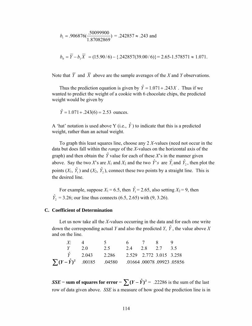
114

)87082869.150099900.(906876.1 =b = .242857 ≈ .243 and

XbYb 10 −= )}6/00.39(242857{.)6/90.15( −= = 2.65-1.578571 ≈ 1.071.

Note that Y and X above are the sample averages of the X and Y observations. Thus the prediction equation is given by XY 243.071.1ˆ += . Thus if we

wanted to predict the weight of a cookie with 6 chocolate chips, the predicted weight would be given by

53.2)6(243.071.1ˆ =+=Y ounces.

A ‘hat’ notation is used above Y (i.e., Y ) to indicate that this is a predicted weight, rather than an actual weight.

To graph this least squares line, choose any 2 X-values (need not occur in the data but does fall within the range of the X-values on the horizontal axis of the graph) and then obtain the Y value for each of these X’s in the manner given above. Say the two X’s are X1 and X2 and the two sY 'ˆ are 1Y and 2Y , then plot the points (X1, 1Y ) and (X2, 2Y ), connect these two points by a straight line. This is the desired line.

For example, suppose X1 = 6.5, then 1Y = 2.65, also setting X2 = 9, then

2Y = 3.26; our line thus connects (6.5, 2.65) with (9, 3.26).

C. Coefficient of Determination

Let us now take all the X-values occurring in the data and for each one write down the corresponding actual Y and also the predicted Y, Y , the value above X and on the line.

X: 4 5 6 7 8 9 Y 2.0 2.5 2.4 2.8 2.7 3.5 Y 2.043 2.286 2.529 2.772 3.015 3.258

∑ − 2)ˆ( YY .00185 .04580 .01664 .00078 .09923 .05856

SSE = sum of squares for error = ∑ − 2)ˆ( YY = .22286 is the sum of the last row of data given above. SSE is a measure of how good the prediction line is in

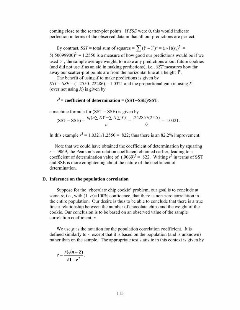
115

coming close to the scatter-plot points. If SSE were 0, this would indicate perfection in terms of the observed data in that all our predictions are perfect.

By contrast, SST = total sum of squares = ∑ − 2)( YY = (n-1)(sy)2 = 5(.50099900)2 = 1.2550 is a measure of how good our predictions would be if we used Y , the sample average weight, to make any predictions about future cookies (and did not use X as an aid in making predictions), i.e., SST measures how far away our scatter-plot points are from the horizontal line at a height Y .

The benefit of using X to make predictions is given by SST − SSE = (1.2550-.22286) = 1.0321 and the proportional gain in using X (over not using X) is given by

r2 = coefficient of determination = (SST−SSE)/SST;

a machine formula for (SST − SSE) is given by

(SST − SSE) = n

YXXYnb ∑ ∑∑ − )(1 = 6

)5.25(242857. = 1.0321.

In this example r2 = 1.0321/1.2550 = .822; thus there is an 82.2% improvement.

Note that we could have obtained the coefficient of determination by squaring r = .9069, the Pearson’s correlation coefficient obtained earlier, leading to a coefficient of determination value of (.9069)2 = .822. Writing r2 in terms of SST and SSE is more enlightening about the nature of the coefficient of determination.

D. Inference on the population correlation

Suppose for the ‘chocolate chip cookie’ problem, our goal is to conclude at some α, i.e., with (1−α)×100% confidence, that there is non-zero correlation in the entire population. Our desire is thus to be able to conclude that there is a true linear relationship between the number of chocolate chips and the weight of the cookie. Our conclusion is to be based on an observed value of the sample correlation coefficient, r.

We use ρ as the notation for the population correlation coefficient. It is

defined similarly to r, except that it is based on the population (and is unknown) rather than on the sample. The appropriate test statistic in this context is given by

21

)2(

r

nrt−

−= .

116

The further r is away from 0, the further t is away from 0 and the more evidence we have that there is a true linear relationship and thus that ρ ≠ 0. Let us use α = .02 for this example.

Note that in this regression context the appropriate df for the t statistic is (n-2). This is so because we are in the ‘simple linear regression’ framework, where we predict one single dependent variable Y from a single independent variable X. To make predictions it is necessary to estimate two quantities from our sample data, the slope and the y-intercept, and to determine the df, we subtract from the sample size, the number of quantities that are needed to make predictions; thus the appropriate df = n - 2. Solution 1st Step:

In formulaic terms, Ha: ρ ≠ 0 versus H0: ρ = 0,

represents the two opposing points of view. 2nd Step:

The appropriate test statistic given above is evaluated as

29069.1)26(9069.

−

−=t = 4.305.

The Decision-Rule approach yields:

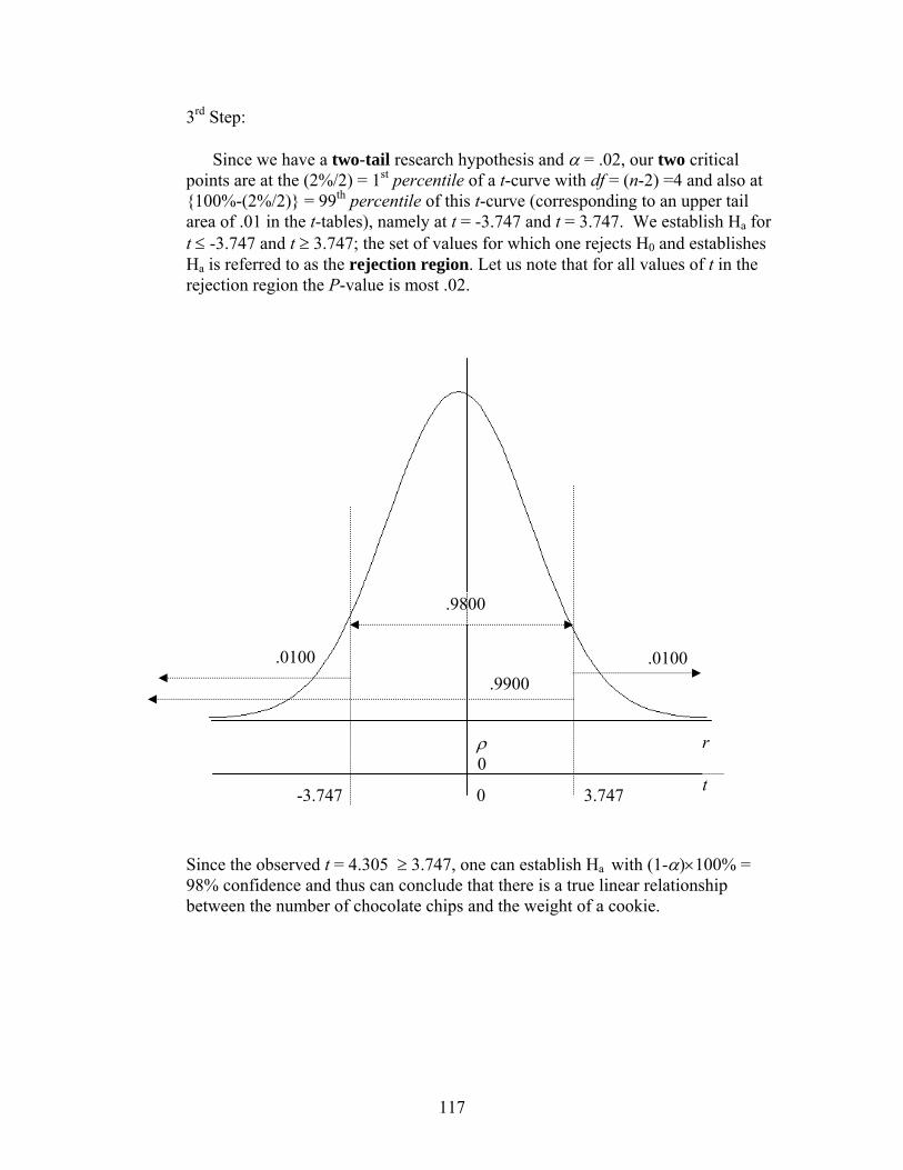
117

3rd Step: Since we have a two-tail research hypothesis and α = .02, our two critical

points are at the (2%/2) = 1st percentile of a t-curve with df = (n-2) =4 and also at {100%-(2%/2)} = 99th percentile of this t-curve (corresponding to an upper tail area of .01 in the t-tables), namely at t = -3.747 and t = 3.747. We establish Ha for t ≤ -3.747 and t ≥ 3.747; the set of values for which one rejects H0 and establishes Ha is referred to as the rejection region. Let us note that for all values of t in the rejection region the P-value is most .02.

Since the observed t = 4.305 ≥ 3.747, one can establish Ha with (1-α)×100% = 98% confidence and thus can conclude that there is a true linear relationship between the number of chocolate chips and the weight of a cookie.

ρ 0

r

t 0 -3.747 3.747

.9900 .0100

.9800

.0100

118

E. Problems 1. We list for 11 printers, their cost (C, in hundreds of dollars) and their rating

(R, on a scale from 0-100). The results are

C 4 5 2.5 2 4 2.85 2.1 2.5 2 1.8 1.3 R 90 90 85 83 78 78 75 70 68 63 61

(NOTE: ΣC = 30.050, ΣC2 = 94.963, ΣR = 841.00, ΣR2 = 65321, ΣCR = 2384.0, sC = 1.135, sR = 10.11) a. Obtain the ‘best’ straight line for predicting the rating of the printer from

its cost by (i) evaluating the slope of the line, (ii) evaluating the y-intercept of the line, (iii) writing down the equation of the straight line.

b. Evaluate the correlation between ‘cost’ and ‘rating’. c. Use the above straight line to predict the rating of a printer that costs 3 (in

hundreds of dollars). d. Can one conclude at α = .01, i.e., with at least 99% confidence, that there

is a linear relationship between the cost of a computer and its rating? Please show your work.

119

2. It is thought that a person’s starting salary is related to the person’s number of years of education beyond high school. The table below gives the indicated information for a random sample of new employees:

Years of Education Beyond High School

1 2 3 4 5 6

Starting Salary (in tens of thousands of dollars)

20 25 24 28 27 35

a. Construct a scatter diagram for these data. b. Find the slope and y-intercept of the regression line for predicting the

starting salary of a new employee from the employee’s number of years of education beyond high school.

c. Find and interpret the coefficient of determination for these data.

3. A commuter would like to predict weekly commuting expense from commuting distance. He interviewed a random sample of 5 commuters and obtained their commuting distances and expenses as indicated in the table below:

Commuting

Distance (miles) Weekly

Commuting Expense (dollars)

10 20 20 30 30 35 40 50 50 55

a. Construct a scatter diagram for these data. b. Find the slope and y-intercept of the regression line for predicting the

weekly commuting expense from the commuting distance.

120

c. Find the coefficient of determination. What percentage of the variation in weekly commuting expense can be explained by a linear association with commuting distance?

4. A firm is interested in predicting its managerial demand. It is believed that there is a relationship between managerial demand and sales. The table below gives the monthly sales (in number of units sold) and the number of mangers needed for a sample of six months:

Monthly Sales (units) 4 5 6 7 8 9 Number of Managers 11 10 12 15 13 16

a. Construct a scatter diagram for these data. b. Find the slope and y-intercept of the regression line for predicting the

number of managers needed from anticipated monthly sales. c. Is there a linear relation between monthly sales and the number of

managers needed? Test appropriate hypotheses at the 5% significance level.

d. Find and interpret the coefficient of determination for these data.

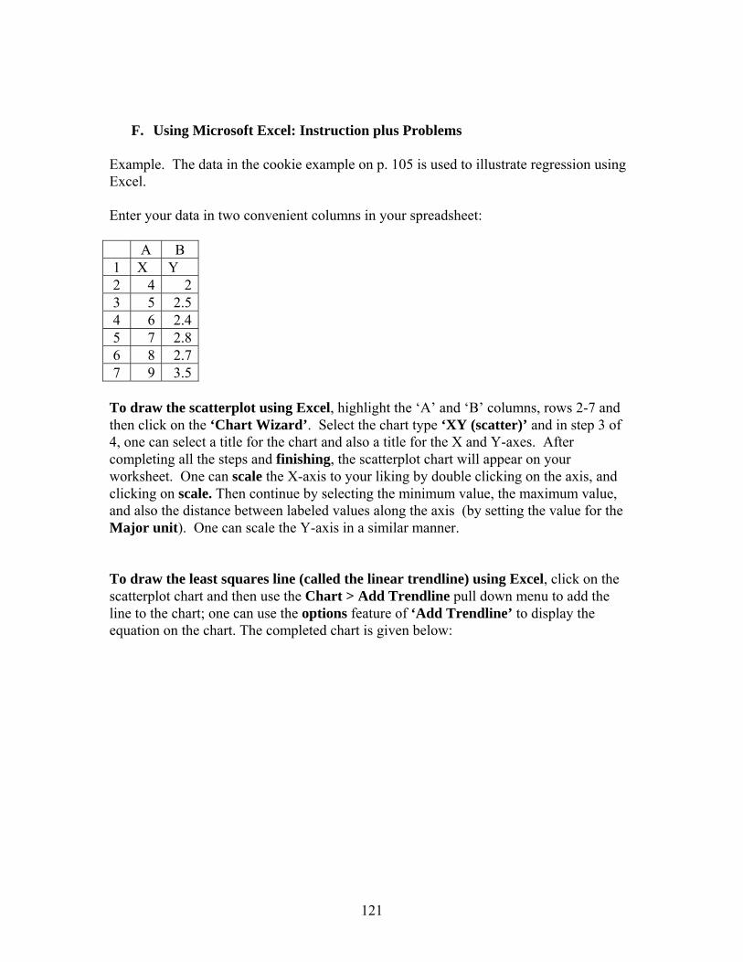
121

F. Using Microsoft Excel: Instruction plus Problems

Example. The data in the cookie example on p. 105 is used to illustrate regression using Excel. Enter your data in two convenient columns in your spreadsheet: A B 1 X Y 2 4 2 3 5 2.5 4 6 2.4 5 7 2.8 6 8 2.7 7 9 3.5 To draw the scatterplot using Excel, highlight the ‘A’ and ‘B’ columns, rows 2-7 and then click on the ‘Chart Wizard’. Select the chart type ‘XY (scatter)’ and in step 3 of 4, one can select a title for the chart and also a title for the X and Y-axes. After completing all the steps and finishing, the scatterplot chart will appear on your worksheet. One can scale the X-axis to your liking by double clicking on the axis, and clicking on scale. Then continue by selecting the minimum value, the maximum value, and also the distance between labeled values along the axis (by setting the value for the Major unit). One can scale the Y-axis in a similar manner. To draw the least squares line (called the linear trendline) using Excel, click on the scatterplot chart and then use the Chart > Add Trendline pull down menu to add the line to the chart; one can use the options feature of ‘Add Trendline’ to display the equation on the chart. The completed chart is given below:

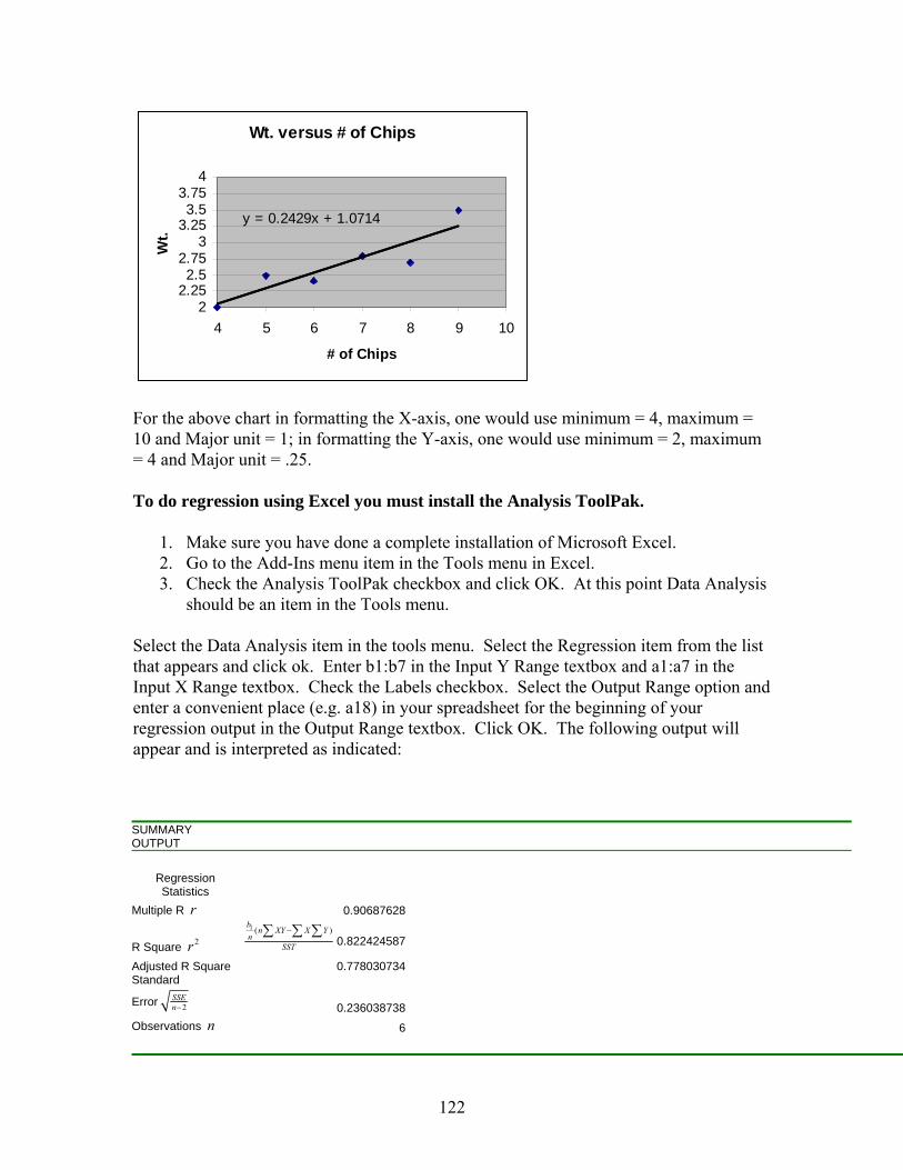
122

For the above chart in formatting the X-axis, one would use minimum = 4, maximum = 10 and Major unit = 1; in formatting the Y-axis, one would use minimum = 2, maximum = 4 and Major unit = .25. To do regression using Excel you must install the Analysis ToolPak. 1. Make sure you have done a complete installation of Microsoft Excel.

2. Go to the Add-Ins menu item in the Tools menu in Excel. 3. Check the Analysis ToolPak checkbox and click OK. At this point Data Analysis

should be an item in the Tools menu. Select the Data Analysis item in the tools menu. Select the Regression item from the list that appears and click ok. Enter b1:b7 in the Input Y Range textbox and a1:a7 in the Input X Range textbox. Check the Labels checkbox. Select the Output Range option and enter a convenient place (e.g. a18) in your spreadsheet for the beginning of your regression output in the Output Range textbox. Click OK. The following output will appear and is interpreted as indicated: SUMMARY OUTPUT

Regression Statistics

Multiple R r 0.90687628

R Square 2r

1 ( )b

n XY X Yn

SST

−∑ ∑ ∑0.822424587

Adjusted R Square 0.778030734 Standard

Error 2SSEn− 0.236038738

Observations n 6

Wt. versus # of Chips

y = 0.2429x + 1.0714

22.252.5

2.753

3.253.5

3.754

4 5 6 7 8 9 10

# of Chips

Wt.

123

ANOVA

df SS MS F Significance F (p value)

Regression 11 ( )b n XY X Y

n−∑ ∑ ∑ 1.032142857

1.032143( 2t )18.52564 0.012604255 Residual 4 ( SSE ) 0.222857143 0.055714

Total 5 ( SST ) 1.255

Coefficients Standard Error t Stat P-value Lower 95% Upper 95%

Intercept ( 0b )1.071428571 0.379204323 2.825465 0.047563 0.018586405 2.12427074

X ( 1b )0.242857143 0.05642405 ( t )4.304142 0.012604 0.08619854 0.39951575

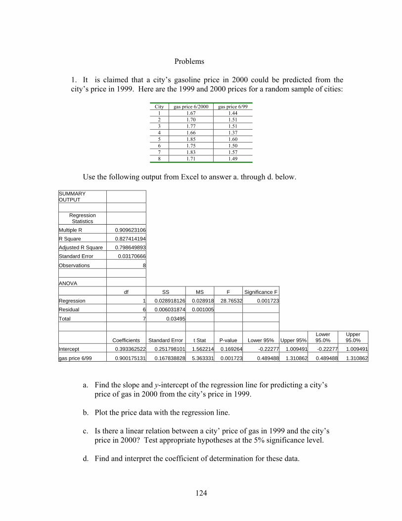
124

Problems

1. It is claimed that a city’s gasoline price in 2000 could be predicted from the

city’s price in 1999. Here are the 1999 and 2000 prices for a random sample of cities:

City gas price 6/2000 gas price 6/99 1 1.67 1.44 2 1.70 1.51 3 1.77 1.51 4 1.66 1.37 5 1.85 1.60 6 1.75 1.50 7 1.83 1.57 8 1.71 1.49

Use the following output from Excel to answer a. through d. below.

SUMMARY OUTPUT

Regression Statistics

Multiple R 0.909623106R Square 0.827414194Adjusted R Square 0.798649893Standard Error 0.03170666

Observations 8

ANOVA df SS MS F Significance F

Regression 1 0.028918126 0.028918 28.76532 0.001723Residual 6 0.006031874 0.001005

Total 7 0.03495

Coefficients Standard Error t Stat P-value Lower 95% Upper 95% Lower 95.0%

Upper 95.0%

Intercept 0.393362522 0.251798101 1.562214 0.169264 -0.22277 1.009491 -0.22277 1.009491

gas price 6/99 0.900175131 0.167838828 5.363331 0.001723 0.489488 1.310862 0.489488 1.310862

a. Find the slope and y-intercept of the regression line for predicting a city’s price of gas in 2000 from the city’s price in 1999.

b. Plot the price data with the regression line.

c. Is there a linear relation between a city’ price of gas in 1999 and the city’s

price in 2000? Test appropriate hypotheses at the 5% significance level.

d. Find and interpret the coefficient of determination for these data.

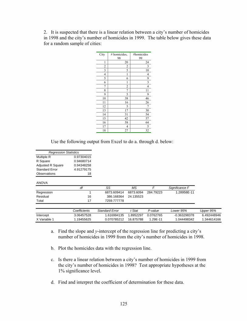
125

2. It is suspected that there is a linear relation between a city’s number of homicides in 1998 and the city’s number of homicides in 1999. The table below gives these data for a random sample of cities:

City # homicides,

98 #homicides

99 1 20 24 2 2 3 3 5 10 4 1 4 5 6 9 6 1 3 7 2 4 8 7 11 9 5 9

10 38 46 11 16 26 12 5 7 13 17 30 14 31 54 15 42 57 16 58 64 17 4 5 18 27 32

Use the following output from Excel to do a. through d. below:

Regression Statistics Multiple R 0.97304015 R Square 0.94680714 Adjusted R Square 0.94348258 Standard Error 4.91279175 Observations 18

ANOVA

df SS MS F Significance F Regression 1 6873.609414 6873.6094 284.79223 1.28958E-11 Residual 16 386.168364 24.135523 Total 17 7259.777778

Coefficients Standard Error t Stat P-value Lower 95% Upper 95%

Intercept 3.06457528 1.616994135 1.8952297 0.0762765 -0.363298378 6.492448946X Variable 1 1.19455625 0.070785212 16.875788 1.29E-11 1.044498342 1.344614166

a. Find the slope and y-intercept of the regression line for predicting a city’s

number of homicides in 1999 from the city’s number of homicides in 1998. b. Plot the homicides data with the regression line. c. Is there a linear relation between a city’s number of homicides in 1999 from

the city’s number of homicides in 1998? Test appropriate hypotheses at the 1% significance level.

d. Find and interpret the coefficient of determination for these data.

126

G. Applications Plus Problems Relating to Capital Asset Pricing Model and

Autoregression

INTRODUCTION to CAPM

An investor when presented with two investment portfolios of equal expected return will choose the portfolio with the lower volatility. Alternatively, an investor presented with two investment portfolios of similar volatility will choose the portfolio with the higher expected return.

If one studied all possible portfolios, there would exist a set of portfolios that had the minimum volatility for a given expected return. This set of portfolios is known as the efficient frontier.

One method of measuring volatility is the standard deviation. Another popular measure of volatility is Beta, which is determined from the Capital Asset Pricing Model (CAPM). Oftentimes the word 'risk' is used interchangeably with the word 'volatility'. CAPITAL ASSET PRICING MODEL

This CAPM theory says that the relationship between the market and a stock can represented by a simple linear regression model: (A-RF) = α + β(M-RF) + ε M = market rate of return (usually S&P 500) RF = risk free rate of return (usually t-bills) A = asset or portfolio of interest ε is unexplained error which follows a Normal Distribution under the model with μ = 0 and σ constant.

In this model, we calculate the least-square line by letting Y=(A-RF) and X=(M-RF) so that Y = a +bx

In this model, b (sometimes called beta) measures the risk of the asset: Beta < 1 means less risk than market Beta = 1 means same risk as market Beta > 1 means more risk than market a (sometimes called alpha) measures performance, relative to similar risk assets. Quite often, this is forced to be zero in finding the least-square line. r2 is used to measure diversification. A pure index fund would have an r2 = 1.

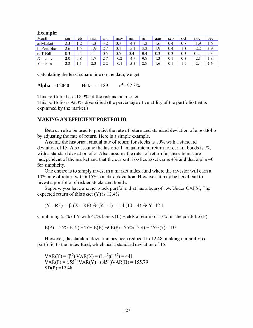
127

Example: Month jan feb mar apr may jun jul aug sep oct nov dec a. Market 2.3 1.2 -1.3 3.2 0.3 -4.3 1.2 1.6 0.4 0.8 -1.9 1.6 b. Portfolio 2.6 1.5 -1.9 2.7 0.4 -5.1 3.2 1.9 0.4 1.3 -2.2 2.9 c. T-Bill 0.3 0.4 0.4 0.5 0.5 0.4 0.4 0.3 0.3 0.3 0.2 0.3 X = a – c 2.0 0.8 -1.7 2.7 -0.2 -4.7 0.8 1.3 0.1 0.5 -2.1 1.3 Y = b - c 2.3 1.1 -2.3 2.2 -0.1 -5.5 2.8 1.6 0.1 1.0 -2.4 2.6 Calculating the least square line on the data, we get Alpha = 0.2040 Beta = 1.189 r2= 92.3% This portfolio has 118.9% of the risk as the market This portfolio is 92.3% diversified (the percentage of volatility of the portfolio that is explained by the market.) MAKING AN EFFICIENT PORTFOLIO

Beta can also be used to predict the rate of return and standard deviation of a portfolio by adjusting the rate of return. Here is a simple example.

Assume the historical annual rate of return for stocks is 10% with a standard deviation of 15. Also assume the historical annual rate of return for certain bonds is 7% with a standard deviation of 5. Also, assume the rates of return for these bonds are independent of the market and that the current risk-free asset earns 4% and that alpha =0 for simplicity.

One choice is to simply invest in a market index fund where the investor will earn a 10% rate of return with a 15% standard deviation. However, it may be beneficial to invest a portfolio of riskier stocks and bonds.

Suppose you have another stock portfolio that has a beta of 1.4. Under CAPM, The expected return of this asset (Y) is 12.4% (Y – RF) = β (X – RF) (Y – 4) = 1.4 (10 – 4) Y=12.4 Combining 55% of Y with 45% bonds (B) yields a return of 10% for the portfolio (P). E(P) = 55% E(Y) +45% E(B) E(P) =55%(12.4) + 45%(7) = 10

However, the standard deviation has been reduced to 12.48, making it a preferred portfolio to the index fund, which has a standard deviation of 15. VAR(Y) = (β2) VAR(X) = (1.42)(152) = 441

VAR(P) = (.552 )VAR(Y)+ (.452 )VAR(B) = 155.79 SD(P) =12.48

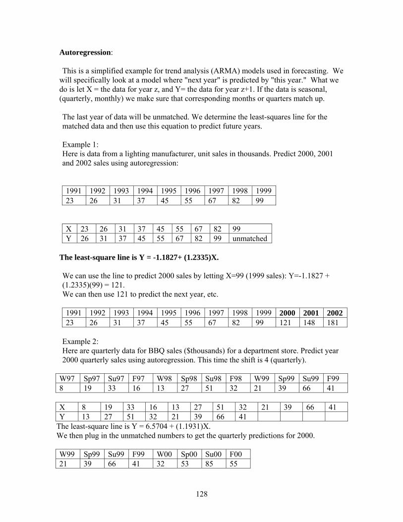
128

Autoregression: This is a simplified example for trend analysis (ARMA) models used in forecasting. We

will specifically look at a model where "next year" is predicted by "this year." What we do is let X = the data for year z, and Y= the data for year z+1. If the data is seasonal, (quarterly, monthly) we make sure that corresponding months or quarters match up. The last year of data will be unmatched. We determine the least-squares line for the matched data and then use this equation to predict future years. Example 1: Here is data from a lighting manufacturer, unit sales in thousands. Predict 2000, 2001 and 2002 sales using autoregression:

1991 1992 1993 1994 1995 1996 1997 1998 1999 23 26 31 37 45 55 67 82 99

X 23 26 31 37 45 55 67 82 99 Y 26 31 37 45 55 67 82 99 unmatched

The least-square line is Y = -1.1827+ (1.2335)X. We can use the line to predict 2000 sales by letting X=99 (1999 sales): Y=-1.1827 + (1.2335)(99) = 121. We can then use 121 to predict the next year, etc. 1991 1992 1993 1994 1995 1996 1997 1998 1999 2000 2001 2002 23 26 31 37 45 55 67 82 99 121 148 181

Example 2: Here are quarterly data for BBQ sales ($thousands) for a department store. Predict year 2000 quarterly sales using autoregression. This time the shift is 4 (quarterly).

W97 Sp97 Su97 F97 W98 Sp98 Su98 F98 W99 Sp99 Su99 F99 8 19 33 16 13 27 51 32 21 39 66 41

X 8 19 33 16 13 27 51 32 21 39 66 41 Y 13 27 51 32 21 39 66 41

The least-square line is Y = 6.5704 + (1.1931)X. We then plug in the unmatched numbers to get the quarterly predictions for 2000. W99 Sp99 Su99 F99 W00 Sp00 Su00 F00 21 39 66 41 32 53 85 55

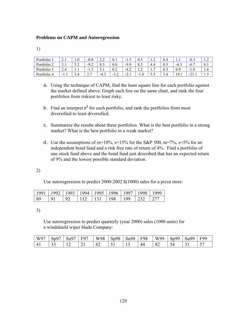
129

Problems on CAPM and Autoregression 1) Portfolio 1 2.1 1.0 -0.8 2.2 0.1 -1.5 0.5 1.2 0.4 1.1 -0.3 1.2 Portfolio 2 3.1 3.2 -9.2 8.3 0.0 -9.9 8.5 4.4 0.5 -4.3 -6.7 8.1 Portfolio 3 2.4 1.1 -1.3 3.1 0.2 -4.2 1.2 1.7 0.3 0.9 -1.8 1.6 Portfolio 4 -1.1 3.4 2.7 -4.3 -3.2 -2.1 -1.0 5.5 3.4 19.1 -21.1 1.5

a. Using the technique of CAPM, find the least square line for each portfolio against the market defined above. Graph each line on the same chart, and rank the four portfolios from riskiest to least risky.

b. Find an interpret r2 for each portfolio, and rank the portfolios from most

diversified to least diversified.

c. Summarize the results about these portfolios. What is the best portfolio in a strong market? What is the best portfolio in a weak market?

d. Use the assumptions of m=10%, s=15% for the S&P 500, m=7%, s=5% for an

independent bond fund and a risk free rate of return of 4%. Find a portfolio of one stock fund above and the bond fund just described that has an expected return of 9% and the lowest possible standard deviation.

2)

Use autoregression to predict 2000-2002 $(1000) sales for a pizza store: 1991 1992 1993 1994 1995 1996 1997 1998 1999 89 91 92 112 131 198 199 232 277 3)

Use autoregression to predict quarterly (year 2000) sales (1000 units) for a windshield wiper blade Company:

W97 Sp97 Su97 F97 W98 Sp98 Su98 F98 W99 Sp99 Su99 F99 41 33 12 21 62 51 13 44 82 54 31 57

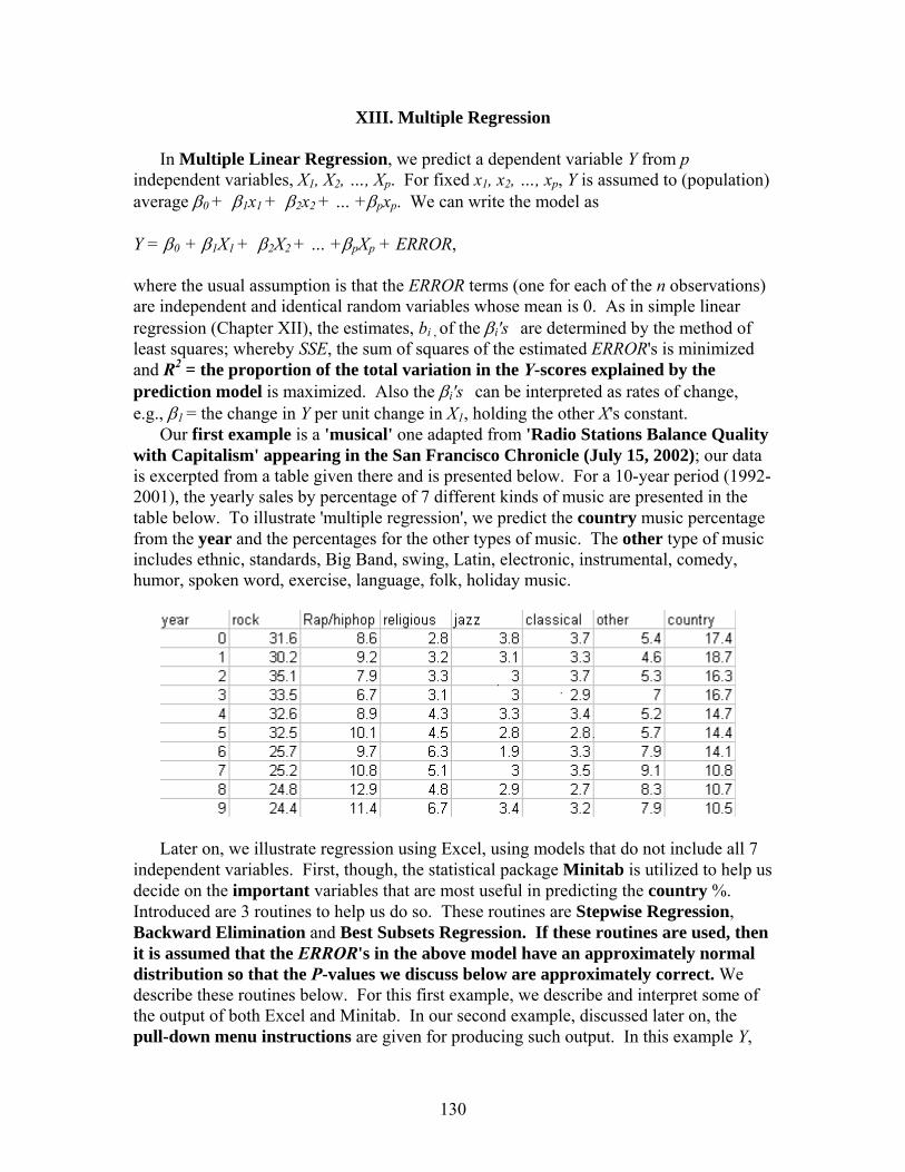
130

XIII. Multiple Regression In Multiple Linear Regression, we predict a dependent variable Y from p

independent variables, X1, X2, …, Xp. For fixed x1, x2, …, xp, Y is assumed to (population) average β0 + β1x1 + β2x2 + … +βpxp. We can write the model as Y = β0 + β1X1 + β2X2 + … +βpXp + ERROR, where the usual assumption is that the ERROR terms (one for each of the n observations) are independent and identical random variables whose mean is 0. As in simple linear regression (Chapter XII), the estimates, bi , of the βi's are determined by the method of least squares; whereby SSE, the sum of squares of the estimated ERROR's is minimized and R2 = the proportion of the total variation in the Y-scores explained by the prediction model is maximized. Also the βi's can be interpreted as rates of change, e.g., β1 = the change in Y per unit change in X1, holding the other X's constant. Our first example is a 'musical' one adapted from 'Radio Stations Balance Quality with Capitalism' appearing in the San Francisco Chronicle (July 15, 2002); our data is excerpted from a table given there and is presented below. For a 10-year period (1992-2001), the yearly sales by percentage of 7 different kinds of music are presented in the table below. To illustrate 'multiple regression', we predict the country music percentage from the year and the percentages for the other types of music. The other type of music includes ethnic, standards, Big Band, swing, Latin, electronic, instrumental, comedy, humor, spoken word, exercise, language, folk, holiday music.

Later on, we illustrate regression using Excel, using models that do not include all 7 independent variables. First, though, the statistical package Minitab is utilized to help us decide on the important variables that are most useful in predicting the country %. Introduced are 3 routines to help us do so. These routines are Stepwise Regression, Backward Elimination and Best Subsets Regression. If these routines are used, then it is assumed that the ERROR's in the above model have an approximately normal distribution so that the P-values we discuss below are approximately correct. We describe these routines below. For this first example, we describe and interpret some of the output of both Excel and Minitab. In our second example, discussed later on, the pull-down menu instructions are given for producing such output. In this example Y,

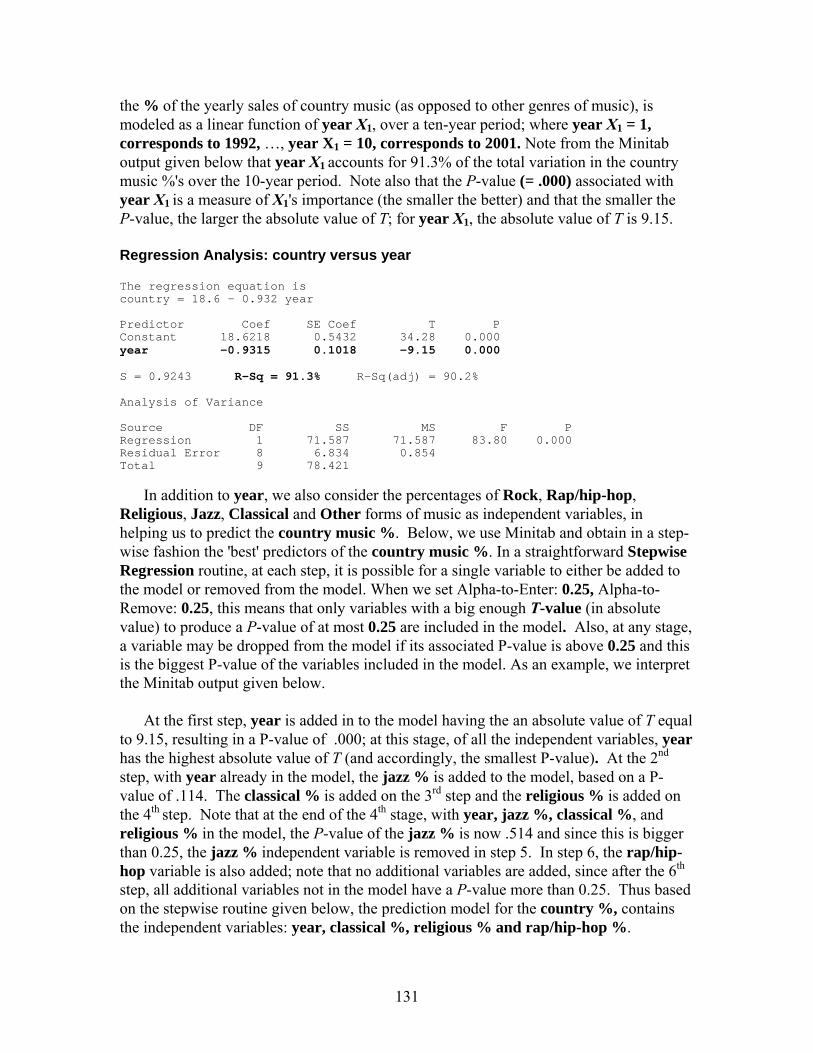
131

the % of the yearly sales of country music (as opposed to other genres of music), is modeled as a linear function of year X1, over a ten-year period; where year X1 = 1, corresponds to 1992, …, year X1 = 10, corresponds to 2001. Note from the Minitab output given below that year X1 accounts for 91.3% of the total variation in the country music %'s over the 10-year period. Note also that the P-value (= .000) associated with year X1 is a measure of X1's importance (the smaller the better) and that the smaller the P-value, the larger the absolute value of T; for year X1, the absolute value of T is 9.15. Regression Analysis: country versus year The regression equation is country = 18.6 - 0.932 year Predictor Coef SE Coef T P Constant 18.6218 0.5432 34.28 0.000 year -0.9315 0.1018 -9.15 0.000 S = 0.9243 R-Sq = 91.3% R-Sq(adj) = 90.2% Analysis of Variance Source DF SS MS F P Regression 1 71.587 71.587 83.80 0.000 Residual Error 8 6.834 0.854 Total 9 78.421

In addition to year, we also consider the percentages of Rock, Rap/hip-hop, Religious, Jazz, Classical and Other forms of music as independent variables, in helping us to predict the country music %. Below, we use Minitab and obtain in a step-wise fashion the 'best' predictors of the country music %. In a straightforward Stepwise Regression routine, at each step, it is possible for a single variable to either be added to the model or removed from the model. When we set Alpha-to-Enter: 0.25, Alpha-to-Remove: 0.25, this means that only variables with a big enough T-value (in absolute value) to produce a P-value of at most 0.25 are included in the model. Also, at any stage, a variable may be dropped from the model if its associated P-value is above 0.25 and this is the biggest P-value of the variables included in the model. As an example, we interpret the Minitab output given below.

At the first step, year is added in to the model having the an absolute value of T equal to 9.15, resulting in a P-value of .000; at this stage, of all the independent variables, year has the highest absolute value of T (and accordingly, the smallest P-value). At the 2nd step, with year already in the model, the jazz % is added to the model, based on a P-value of .114. The classical % is added on the 3rd step and the religious % is added on the 4th step. Note that at the end of the 4th stage, with year, jazz %, classical %, and religious % in the model, the P-value of the jazz % is now .514 and since this is bigger than 0.25, the jazz % independent variable is removed in step 5. In step 6, the rap/hip-hop variable is also added; note that no additional variables are added, since after the 6th step, all additional variables not in the model have a P-value more than 0.25. Thus based on the stepwise routine given below, the prediction model for the country %, contains the independent variables: year, classical %, religious % and rap/hip-hop %.

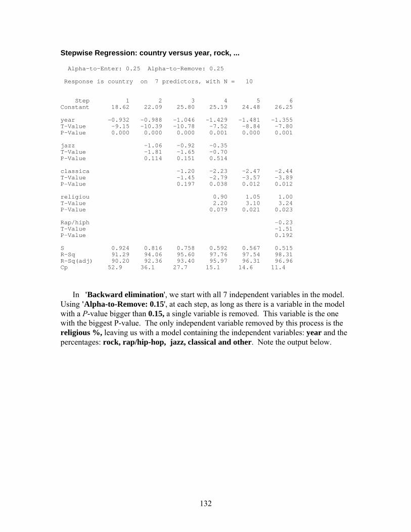
132

Stepwise Regression: country versus year, rock, ... Alpha-to-Enter: 0.25 Alpha-to-Remove: 0.25 Response is country on 7 predictors, with N = 10 Step 1 2 3 4 5 6 Constant 18.62 22.09 25.80 25.19 24.48 26.25 year -0.932 -0.988 -1.046 -1.429 -1.481 -1.355 T-Value -9.15 -10.39 -10.78 -7.52 -8.84 -7.80 P-Value 0.000 0.000 0.000 0.001 0.000 0.001 jazz -1.06 -0.92 -0.35 T-Value -1.81 -1.65 -0.70 P-Value 0.114 0.151 0.514 classica -1.20 -2.23 -2.47 -2.44 T-Value -1.45 -2.79 -3.57 -3.89 P-Value 0.197 0.038 0.012 0.012 religiou 0.90 1.05 1.00 T-Value 2.20 3.10 3.24 P-Value 0.079 0.021 0.023 Rap/hiph -0.23 T-Value -1.51 P-Value 0.192 S 0.924 0.816 0.758 0.592 0.567 0.515 R-Sq 91.29 94.06 95.60 97.76 97.54 98.31 R-Sq(adj) 90.20 92.36 93.40 95.97 96.31 96.96 Cp 52.9 36.1 27.7 15.1 14.6 11.4

In 'Backward elimination', we start with all 7 independent variables in the model. Using 'Alpha-to-Remove: 0.15', at each step, as long as there is a variable in the model with a P-value bigger than 0.15, a single variable is removed. This variable is the one with the biggest P-value. The only independent variable removed by this process is the religious %, leaving us with a model containing the independent variables: year and the percentages: rock, rap/hip-hop, jazz, classical and other. Note the output below.

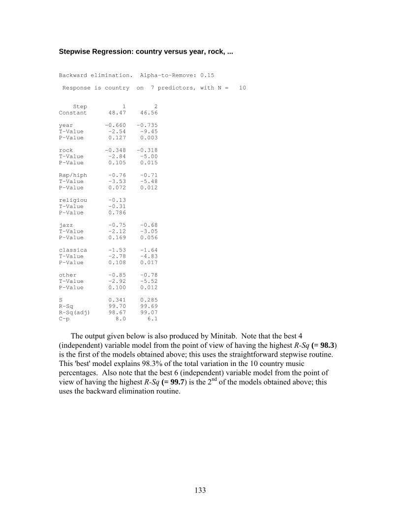
133

Stepwise Regression: country versus year, rock, ... Backward elimination. Alpha-to-Remove: 0.15 Response is country on 7 predictors, with N = 10 Step 1 2 Constant 48.47 46.56 year -0.660 -0.735 T-Value -2.54 -9.45 P-Value 0.127 0.003 rock -0.348 -0.318 T-Value -2.84 -5.00 P-Value 0.105 0.015 Rap/hiph -0.76 -0.71 T-Value -3.53 -5.48 P-Value 0.072 0.012 religiou -0.13 T-Value -0.31 P-Value 0.786 jazz -0.75 -0.68 T-Value -2.12 -3.05 P-Value 0.169 0.056 classica -1.53 -1.64 T-Value -2.78 -4.83 P-Value 0.108 0.017 other -0.85 -0.78 T-Value -2.92 -5.52 P-Value 0.100 0.012 S 0.341 0.285 R-Sq 99.70 99.69 R-Sq(adj) 98.67 99.07 C-p 8.0 6.1

The output given below is also produced by Minitab. Note that the best 4

(independent) variable model from the point of view of having the highest R-Sq (= 98.3) is the first of the models obtained above; this uses the straightforward stepwise routine. This 'best' model explains 98.3% of the total variation in the 10 country music percentages. Also note that the best 6 (independent) variable model from the point of view of having the highest R-Sq (= 99.7) is the 2nd of the models obtained above; this uses the backward elimination routine.

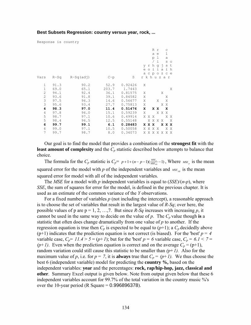
134

Best Subsets Regression: country versus year, rock, ... Response is country R r c a e l p l a / i s o y r h g j s t e o i i a i h a c p o z c e Vars R-Sq R-Sq(adj) C-p S r k h u z a r 1 91.3 90.2 52.9 0.92426 X 1 69.0 65.1 203.7 1.7443 X 2 94.1 92.4 36.1 0.81575 X X 2 93.6 91.8 39.1 0.84582 X X 3 97.5 96.3 14.6 0.56677 X X X 3 95.6 93.4 27.7 0.75813 X X X 4 98.3 97.0 11.4 0.51476 X X X X 4 97.8 96.0 15.1 0.59239 X X X X 5 98.7 97.1 10.6 0.49914 X X X X X 5 98.4 96.5 12.5 0.55148 X X X X X 6 99.7 99.1 6.1 0.28483 X X X X X X 6 99.0 97.1 10.5 0.50058 X X X X X X 7 99.7 98.7 8.0 0.34073 X X X X X X X

Our goal is to find the model that provides a combination of the strongest fit with the least amount of complexity and the Cp statistic described below attempts to balance that choice. The formula for the Cp statistic is Cp=

All1 ( 1)( 1)pMSE

MSEp n p+ + − − − , Where pMSE is the mean squared error for the model with p of the independent variables and AllMSE is the mean squared error for model with all of the independent variables. The MSE for a model with p independent variables is equal to (SSE)/(n-p), where SSE, the sum of squares for error for the model, is defined in the previous chapter. It is used as an estimate of the common variance of the Y observations. For a fixed number of variables p (not including the intercept), a reasonable approach is to choose the set of variables that result in the largest value of R-Sq; over here, the possible values of p are p = 1, 2, …,7. But since R-Sq increases with increasing p, it cannot be used in the same way to decide on the value of p. The Cp value though is a statistic that often does change dramatically from one value of p to another. If the regression equation is true then Cp is expected to be equal to (p+1); a Cp decidedly above (p+1) indicates that the prediction equation is not correct (is biased). For the 'best' p = 4 variable case, Cp= 11.4 > 5 = (p+1); but for the 'best' p = 6 variable case, Cp = 6.1 < 7 = (p+1). Even when the prediction equation is correct and on the average Cp = (p+1), random variation could still cause this statistic to be smaller than (p+1). Also for the maximum value of p, i.e. for p = 7, it is always true that Cp = (p+1). We thus choose the best 6 (independent variable) model for predicting the country %, based on the independent variables: year and the percentages: rock, rap/hip-hop, jazz, classical and other. Summary Excel output is given below. Note from output given below that these 6 independent variables account for 99.7% of the total variation in the country music %'s over the 10-year period (R Square = 0.996896378).

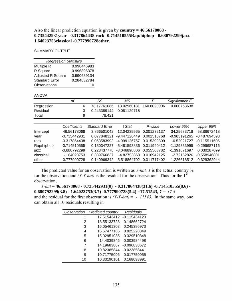
135

Also the linear prediction equation is given by country = 46.56178068 -0.735442931year - 0.317864438 rock -0.714510555Rap/hiphop - 0.680792299jazz - 1.64023753classical -0.777990728other. SUMMARY OUTPUT

Regression Statistics

Multiple R 0.998446983 R Square 0.996896378 Adjusted R Square 0.990689134 Standard Error 0.284832784 Observations 10

ANOVA

df SS MS F Significance F Regression 6 78.17761086 13.02960181 160.6020906 0.000753638Residual 3 0.243389144 0.081129715 Total 9 78.421

Coefficients Standard Error t Stat P-value Lower 95% Upper 95%

Intercept 46.56178068 3.866501042 12.04235565 0.001232137 34.25683718 58.86672418year -0.735442931 0.077848321 -9.447126449 0.002513768 -0.983191265 -0.487694598rock -0.317864438 0.063583993 -4.999126757 0.015399809 -0.52021727 -0.115511606Rap/hiphop -0.714510555 0.130347227 -5.481593836 0.011940412 -1.129333995 -0.299687116jazz -0.680792299 0.223437778 -3.046898806 0.055563782 -1.391871697 0.030287099classical -1.64023753 0.339766837 -4.82753863 0.016942125 -2.72152826 -0.558946801other -0.777990728 0.140969342 -5.518864702 0.011717402 -1.226618512 -0.329362944

The predicted value for an observation is written as Y-hat, Y is the actual country % for the observation and (Y-Y-hat) is the residual for the observation. Thus for the 1st observation,

Y-hat = 46.56178068 - 0.735442931(0) - 0.317864438(31.6) -0.714510555(8.6) - 0.680792299(3.8) - 1.64023753(3.7) -0.777990728(5.4) =17.51543, Y = 17.4 and the residual for the first observation is (Y-Y-hat) = - .11543. In the same way, one can obtain all 10 residuals resulting in

Observation Predicted country Residuals 1 17.51543412 -0.1154341232 18.55133728 0.1486627243 16.05461303 0.2453869734 16.67477165 0.0252283495 15.02951035 -0.3295103486 14.4039845 -0.0039844987 14.19683867 -0.0968386728 10.82385844 -0.0238584419 10.71775096 -0.017750955

10 10.33190101 0.168098991

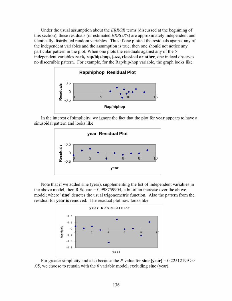
136

Under the usual assumption about the ERROR terms (discussed at the beginning of this section), these residuals (or estimated ERROR's) are approximately independent and identically distributed random variables. Thus if one plotted the residuals against any of the independent variables and the assumption is true, then one should not notice any particular pattern in the plot. When one plots the residuals against any of the 5 independent variables rock, rap/hip-hop, jazz, classical or other, one indeed observes no discernible pattern. For example, for the Rap/hip-hop variable, the graph looks like

In the interest of simplicity, we ignore the fact that the plot for year appears to have a sinusoidal pattern and looks like

Note that if we added sine (year), supplementing the list of independent variables in

the above model, then R Square = 0.998759904, a bit of an increase over the above model; where 'sine' denotes the usual trigonometric function. Also the pattern from the residual for year is removed. The residual plot now looks like

For greater simplicity and also because the P-value for sine (year) = 0.22512199 >> .05, we choose to remain with the 6 variable model, excluding sine (year).

year Residual Plot

-0.5

0

0.5

0 2 4 6 8 10

year

Res

idua

ls

Rap/hiphop Residual Plot

-0.5

0

0.5

0 5 10 15

Rap/hiphop

Res

idua

ls

y e a r R e s id u a l P lo t

-0 . 3

-0 . 2

-0 . 1

0

0 . 1

0 . 2

0 2 4 6 8 1 0

y e a r

Res

idua

ls

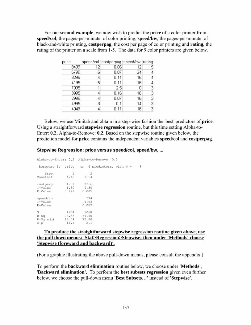
137

For our second example, we now wish to predict the price of a color printer from speed/col, the pages-per-minute of color printing, speed/bw, the pages-per-minute of black-and-white printing, costperpag, the cost per page of color printing and rating, the rating of the printer on a scale from 1-5. The data for 9 color printers are given below.

Below, we use Minitab and obtain in a step-wise fashion the 'best' predictors of price.

Using a straightforward stepwise regression routine, but this time setting Alpha-to-Enter: 0.2, Alpha-to-Remove: 0.2. Based on the stepwise routine given below, the prediction model for price contains the independent variables speed/col and costperpag.

Stepwise Regression: price versus speed/col, speed/bw, ... Alpha-to-Enter: 0.2 Alpha-to-Remove: 0.2 Response is price on 4 predictors, with N = 9 Step 1 2 Constant 4742 1614 costperp 1261 2316 T-Value 1.50 4.30 P-Value 0.177 0.005 speed/co 574 T-Value 4.03 P-Value 0.007 S 1904 1068 R-Sq 24.35 79.60 R-Sq(adj) 13.54 72.80 C-p 14.1 2.1

To produce the straightforward stepwise regression routine given above, use the pull down menus: Stat>Regression>Stepwise; then under 'Methods' choose 'Stepwise (foreward and backward)'. (For a graphic illustrating the above pull-down menus, please consult the appendix.) To perform the backward elimination routine below, we choose under 'Methods', 'Backward elimination'. To perform the best subsets regression given even further below, we choose the pull-down menu 'Best Subsets…' instead of 'Stepwise'.

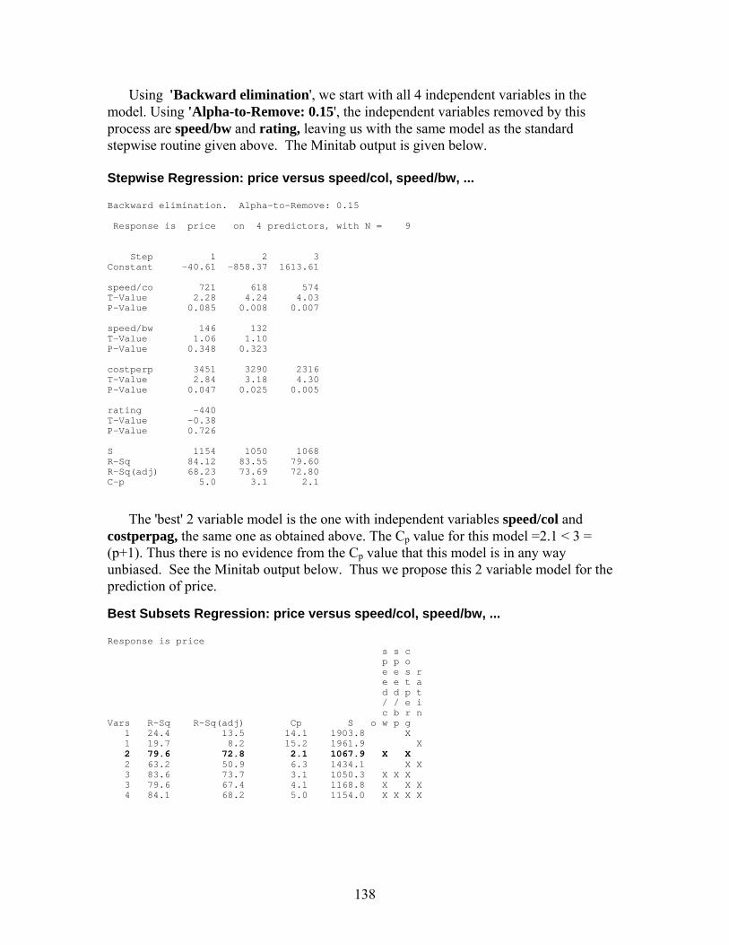
138

Using 'Backward elimination', we start with all 4 independent variables in the model. Using 'Alpha-to-Remove: 0.15', the independent variables removed by this process are speed/bw and rating, leaving us with the same model as the standard stepwise routine given above. The Minitab output is given below. Stepwise Regression: price versus speed/col, speed/bw, ... Backward elimination. Alpha-to-Remove: 0.15 Response is price on 4 predictors, with N = 9 Step 1 2 3 Constant -40.61 -858.37 1613.61 speed/co 721 618 574 T-Value 2.28 4.24 4.03 P-Value 0.085 0.008 0.007 speed/bw 146 132 T-Value 1.06 1.10 P-Value 0.348 0.323 costperp 3451 3290 2316 T-Value 2.84 3.18 4.30 P-Value 0.047 0.025 0.005 rating -440 T-Value -0.38 P-Value 0.726 S 1154 1050 1068 R-Sq 84.12 83.55 79.60 R-Sq(adj) 68.23 73.69 72.80 C-p 5.0 3.1 2.1

The 'best' 2 variable model is the one with independent variables speed/col and costperpag, the same one as obtained above. The Cp value for this model =2.1 < 3 = (p+1). Thus there is no evidence from the Cp value that this model is in any way unbiased. See the Minitab output below. Thus we propose this 2 variable model for the prediction of price.

Best Subsets Regression: price versus speed/col, speed/bw, ... Response is price s s c p p o e e s r e e t a d d p t / / e i c b r n Vars R-Sq R-Sq(adj) Cp S o w p g 1 24.4 13.5 14.1 1903.8 X 1 19.7 8.2 15.2 1961.9 X 2 79.6 72.8 2.1 1067.9 X X 2 63.2 50.9 6.3 1434.1 X X 3 83.6 73.7 3.1 1050.3 X X X 3 79.6 67.4 4.1 1168.8 X X X 4 84.1 68.2 5.0 1154.0 X X X X

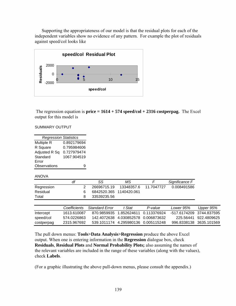
139

Supporting the appropriateness of our model is that the residual plots for each of the independent variables show no evidence of any pattern. For example the plot of residuals against speed/col looks like

The regression equation is price = 1614 + 574 speed/col + 2316 costperpag. The Excel output for this model is SUMMARY OUTPUT

Regression Statistics

Multiple R 0.892179694 R Square 0.795984606 Adjusted R Sq 0.727979474 Standard Error

1067.904519

Observations 9

ANOVA df SS MS F Significance F

Regression 2 26696715.19 13348357.6 11.7047727 0.008491586Residual 6 6842520.365 1140420.061 Total 8 33539235.56

Coefficients Standard Error t Stat P-value Lower 95% Upper 95%

Intercept 1613.610087 870.9859935 1.852624611 0.113376924 -517.6174209 3744.837595speed/col 574.0226863 142.4072638 4.030852578 0.006873632 225.56441 922.4809625costperpag 2315.967692 539.1011174 4.295980136 0.005115248 996.8338138 3635.101569 The pull down menus: Tools>Data Analysis>Regression produce the above Excel output. When one is entering information in the Regression dialogue box, check Residuals, Residual Plots and Normal Probability Plots; also assuming the names of the relevant variables are included in the range of these variables (along with the values), check Labels. (For a graphic illustrating the above pull-down menus, please consult the appendix.)

speed/col Residual Plot

-2000

0

2000

0 5 10 15

speed/col

Res

idua

ls

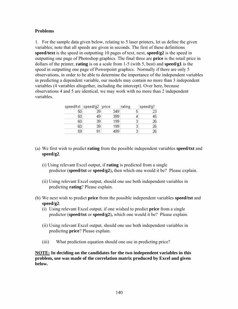
140

Problems 1. For the sample data given below, relating to 5 laser printers, let us define the given variables; note that all speeds are given in seconds. The first of these definitions speed/text is the speed in outputting 10 pages of text, next, speed/g2 is the speed in outputting one page of Photoshop graphics. The final three are price is the retail price in dollars of the printer, rating is on a scale from 1-5 (with 5, best) and speed/g1 is the speed in outputting one page of Powerpoint graphics. Normally if there are only 5 observations, in order to be able to determine the importance of the independent variables in predicting a dependent variable, our models may contain no more than 3 independent variables (4 variables altogether, including the intercept). Over here, because observations 4 and 5 are identical, we may work with no more than 2 independent variables.

(a) We first wish to predict rating from the possible independent variables speed/txt and

speed/g2.

(i) Using relevant Excel output, if rating is predicted from a single predictor (speed/txt or speed/g2), then which one would it be? Please explain.

(ii) Using relevant Excel output, should one use both independent variables in predicting rating? Please explain.

(b) We next wish to predict price from the possible independent variables speed/txt and speed/g2.

(i) Using relevant Excel output, if one wished to predict price from a single predictor (speed/txt or speed/g2), which one would it be? Please explain.

(ii) Using relevant Excel output, should one use both independent variables in predicting price? Please explain.

(iii) What prediction equation should one use in predicting price? NOTE: In deciding on the candidates for the two independent variables in this problem, use was made of the correlation matrix produced by Excel and given below.

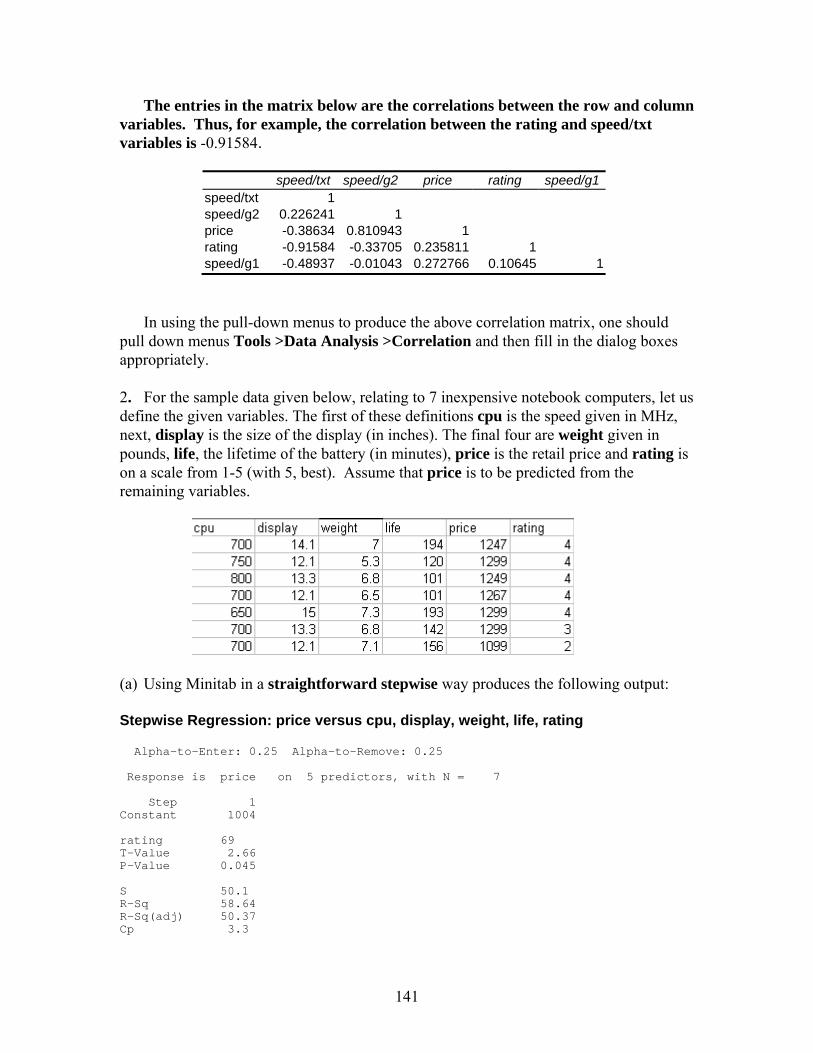
141

The entries in the matrix below are the correlations between the row and column variables. Thus, for example, the correlation between the rating and speed/txt variables is -0.91584.

speed/txt speed/g2 price rating speed/g1 speed/txt 1 speed/g2 0.226241 1 price -0.38634 0.810943 1 rating -0.91584 -0.33705 0.235811 1 speed/g1 -0.48937 -0.01043 0.272766 0.10645 1

In using the pull-down menus to produce the above correlation matrix, one should pull down menus Tools >Data Analysis >Correlation and then fill in the dialog boxes appropriately. 2. For the sample data given below, relating to 7 inexpensive notebook computers, let us define the given variables. The first of these definitions cpu is the speed given in MHz, next, display is the size of the display (in inches). The final four are weight given in pounds, life, the lifetime of the battery (in minutes), price is the retail price and rating is on a scale from 1-5 (with 5, best). Assume that price is to be predicted from the remaining variables.

(a) Using Minitab in a straightforward stepwise way produces the following output: Stepwise Regression: price versus cpu, display, weight, life, rating Alpha-to-Enter: 0.25 Alpha-to-Remove: 0.25 Response is price on 5 predictors, with N = 7 Step 1 Constant 1004 rating 69 T-Value 2.66 P-Value 0.045 S 50.1 R-Sq 58.64 R-Sq(adj) 50.37 Cp 3.3

142

Write down the linear model suggested by this output for predicting price.

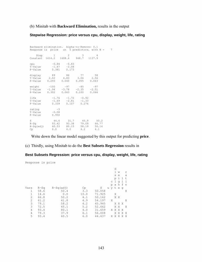
143

(b) Minitab with Backward Elimination, results in the output Stepwise Regression: price versus cpu, display, weight, life, rating Backward elimination. Alpha-to-Remove: 0.1 Response is price on 5 predictors, with N = 7 Step 1 2 3 4 Constant 1614.2 1608.4 948.7 1137.9 cpu -0.84 -0.83 T-Value -1.47 -2.08 P-Value 0.381 0.173 display 89 86 77 58 T-Value 2.02 4.83 3.06 2.56 P-Value 0.293 0.040 0.055 0.063 weight -100 -97 -85 -97 T-Value -1.94 -3.78 -2.35 -2.51 P-Value 0.302 0.063 0.100 0.066 life -1.76 -1.72 -0.92 T-Value -1.69 -2.81 -1.33 P-Value 0.339 0.107 0.276 rating -3 T-Value -0.08 P-Value 0.950 S 44.6 31.7 45.9 50.2 R-Sq 93.42 93.38 79.09 66.77 R-Sq(adj) 60.53 80.15 58.19 50.16 Cp 6.0 4.0 4.2 4.1

Write down the linear model suggested by this output for predicting price. (c) Thirdly, using Minitab to do the Best Subsets Regression results in Best Subsets Regression: price versus cpu, display, weight, life, rating Response is price d i w r s e a p i l t c l g i i p a h f n Vars R-Sq R-Sq(adj) Cp S u y t e g 1 58.6 50.4 3.3 50.058 X 1 14.6 0.0 10.0 71.925 X 2 66.8 50.2 4.1 50.162 X X 2 61.2 41.8 4.9 54.197 X X 3 79.1 58.2 4.2 45.945 X X X 3 72.5 45.1 5.2 52.662 X X X 4 93.4 80.1 4.0 31.659 X X X X 4 79.3 37.9 6.1 56.008 X X X X 5 93.4 60.5 6.0 44.637 X X X X X

143

From an (R-Sq/C-p) point of view, write down the suggested prediction equation for predicting price; please explain. From an intuitive point of view, does this equation seem totally reasonable? Please explain. (d) Choose your favorite model and support this choice. Obtain the Excel output for this

model and comment on the behavior of the observed residuals and if they seem to support the assumptions made about them.

General Comments 1) The second example described earlier was adapted from 'Ultrafast Color Printers'

appearing in 'PC Computing' (Mar 1999); our data was excerpted from a table given there.

2) The first and second problems were adapted from 'The Fine Print' (Oct 01) and 'Low-Cost Lightweights' (Sep 01), both appearing in 'Smart Business Magazine'.

3) The correlation matrix for all pairs of variables discussed at the end of problem 1 is

just the Pearson correlation coefficients r, evaluated between pairs of variables as discussed in Chapter XII (Simple Linear Regression: one independent variable); of course r depends on the particular pair of variables. The Multicollinearity situation arises when there is high correlation among some pairs of independent variables; this means that these highly correlated pairs have overlapping information and this introduces ambiguity in determining contributions of individual variables. Multicollinearity is not desirable and should be avoided, if possible.

4) In discussing various routines for choosing 'good' independent variables such as Stepwise Regression, we use 'high' P-values such as .15, .20, .25, whereas in earlier chapters we focused on values closer to .05. Here, the choice is different than the choice of alpha for a hypothesis test because we want to keep variables in the model if they are helpful and using low P-values (at the start) in our routines could result in us overlooking important variables. Later on in deciding among competing models, we may revert to smaller P-values, such as ones closer to .05.

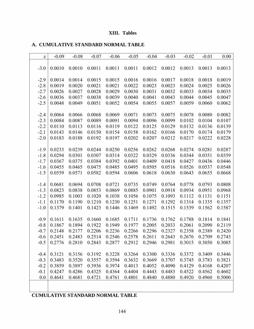
144

XIII. Tables A. CUMULATIVE STANDARD NORMAL TABLE

z -0.09 -0.08 -0.07 -0.06 -0.05 -0.04 -0.03 -0.02 -0.01 0.00

-3.0 0.0010 0.0010 0.0011 0.0011 0.0011 0.0012 0.0012 0.0013 0.0013 0.0013

-2.9 0.0014 0.0014 0.0015 0.0015 0.0016 0.0016 0.0017 0.0018 0.0018 0.0019-2.8 0.0019 0.0020 0.0021 0.0021 0.0022 0.0023 0.0023 0.0024 0.0025 0.0026-2.7 0.0026 0.0027 0.0028 0.0029 0.0030 0.0031 0.0032 0.0033 0.0034 0.0035-2.6 0.0036 0.0037 0.0038 0.0039 0.0040 0.0041 0.0043 0.0044 0.0045 0.0047-2.5 0.0048 0.0049 0.0051 0.0052 0.0054 0.0055 0.0057 0.0059 0.0060 0.0062

-2.4 0.0064 0.0066 0.0068 0.0069 0.0071 0.0073 0.0075 0.0078 0.0080 0.0082-2.3 0.0084 0.0087 0.0089 0.0091 0.0094 0.0096 0.0099 0.0102 0.0104 0.0107-2.2 0.0110 0.0113 0.0116 0.0119 0.0122 0.0125 0.0129 0.0132 0.0136 0.0139-2.1 0.0143 0.0146 0.0150 0.0154 0.0158 0.0162 0.0166 0.0170 0.0174 0.0179-2.0 0.0183 0.0188 0.0192 0.0197 0.0202 0.0207 0.0212 0.0217 0.0222 0.0228

-1.9 0.0233 0.0239 0.0244 0.0250 0.0256 0.0262 0.0268 0.0274 0.0281 0.0287-1.8 0.0294 0.0301 0.0307 0.0314 0.0322 0.0329 0.0336 0.0344 0.0351 0.0359-1.7 0.0367 0.0375 0.0384 0.0392 0.0401 0.0409 0.0418 0.0427 0.0436 0.0446-1.6 0.0455 0.0465 0.0475 0.0485 0.0495 0.0505 0.0516 0.0526 0.0537 0.0548-1.5 0.0559 0.0571 0.0582 0.0594 0.0606 0.0618 0.0630 0.0643 0.0655 0.0668

-1.4 0.0681 0.0694 0.0708 0.0721 0.0735 0.0749 0.0764 0.0778 0.0793 0.0808-1.3 0.0823 0.0838 0.0853 0.0869 0.0885 0.0901 0.0918 0.0934 0.0951 0.0968-1.2 0.0985 0.1003 0.1020 0.1038 0.1056 0.1075 0.1093 0.1112 0.1131 0.1151-1.1 0.1170 0.1190 0.1210 0.1230 0.1251 0.1271 0.1292 0.1314 0.1335 0.1357-1.0 0.1379 0.1401 0.1423 0.1446 0.1469 0.1492 0.1515 0.1539 0.1562 0.1587

-0.9 0.1611 0.1635 0.1660 0.1685 0.1711 0.1736 0.1762 0.1788 0.1814 0.1841-0.8 0.1867 0.1894 0.1922 0.1949 0.1977 0.2005 0.2033 0.2061 0.2090 0.2119-0.7 0.2148 0.2177 0.2206 0.2236 0.2266 0.2296 0.2327 0.2358 0.2389 0.2420-0.6 0.2451 0.2483 0.2514 0.2546 0.2578 0.2611 0.2643 0.2676 0.2709 0.2743-0.5 0.2776 0.2810 0.2843 0.2877 0.2912 0.2946 0.2981 0.3015 0.3050 0.3085

-0.4 0.3121 0.3156 0.3192 0.3228 0.3264 0.3300 0.3336 0.3372 0.3409 0.3446-0.3 0.3483 0.3520 0.3557 0.3594 0.3632 0.3669 0.3707 0.3745 0.3783 0.3821-0.2 0.3859 0.3897 0.3936 0.3974 0.4013 0.4052 0.4090 0.4129 0.4168 0.4207-0.1 0.4247 0.4286 0.4325 0.4364 0.4404 0.4443 0.4483 0.4522 0.4562 0.46020.0 0.4641 0.4681 0.4721 0.4761 0.4801 0.4840 0.4880 0.4920 0.4960 0.5000

CUMULATIVE STANDARD NORMAL TABLE

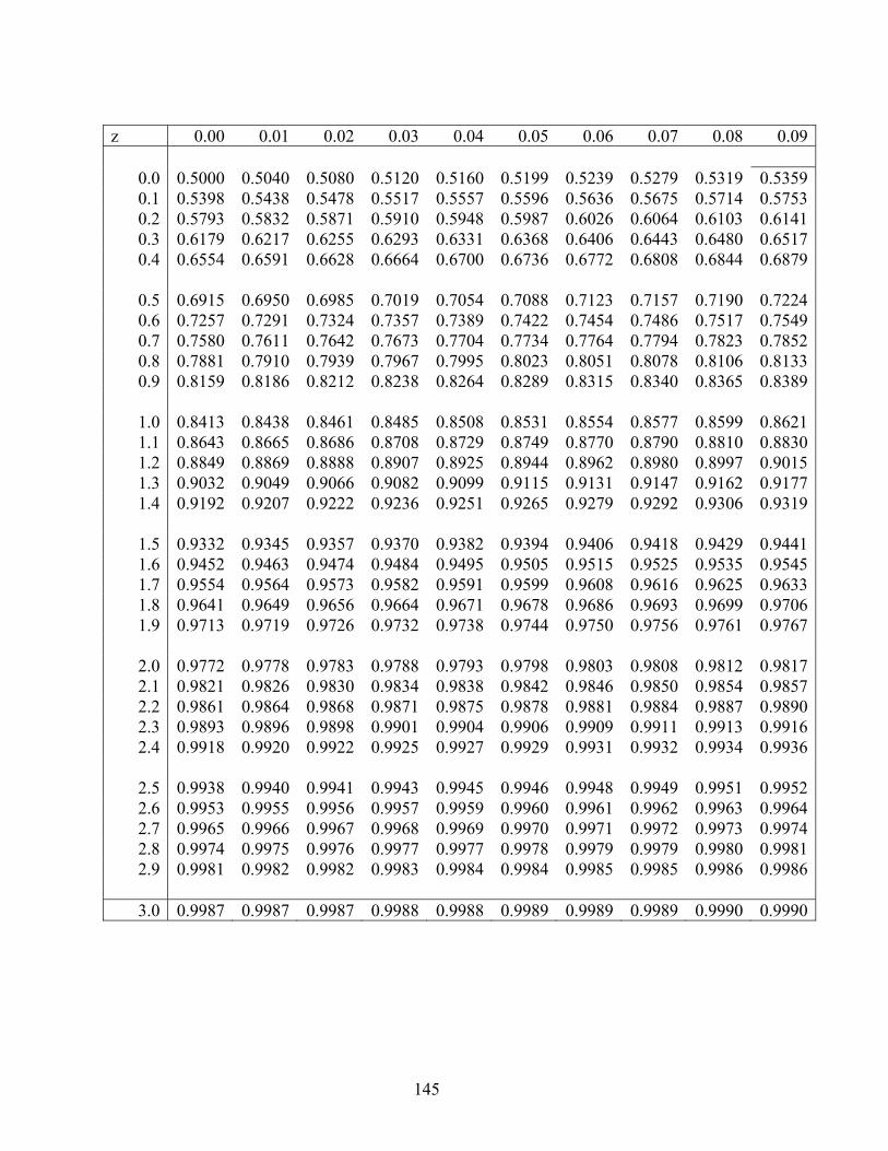
145

z 0.00 0.01 0.02 0.03 0.04 0.05 0.06 0.07 0.08 0.09

0.0 0.5000 0.5040 0.5080 0.5120 0.5160 0.5199 0.5239 0.5279 0.5319 0.53590.1 0.5398 0.5438 0.5478 0.5517 0.5557 0.5596 0.5636 0.5675 0.5714 0.57530.2 0.5793 0.5832 0.5871 0.5910 0.5948 0.5987 0.6026 0.6064 0.6103 0.61410.3 0.6179 0.6217 0.6255 0.6293 0.6331 0.6368 0.6406 0.6443 0.6480 0.65170.4 0.6554 0.6591 0.6628 0.6664 0.6700 0.6736 0.6772 0.6808 0.6844 0.6879

0.5 0.6915 0.6950 0.6985 0.7019 0.7054 0.7088 0.7123 0.7157 0.7190 0.72240.6 0.7257 0.7291 0.7324 0.7357 0.7389 0.7422 0.7454 0.7486 0.7517 0.75490.7 0.7580 0.7611 0.7642 0.7673 0.7704 0.7734 0.7764 0.7794 0.7823 0.78520.8 0.7881 0.7910 0.7939 0.7967 0.7995 0.8023 0.8051 0.8078 0.8106 0.81330.9 0.8159 0.8186 0.8212 0.8238 0.8264 0.8289 0.8315 0.8340 0.8365 0.8389

1.0 0.8413 0.8438 0.8461 0.8485 0.8508 0.8531 0.8554 0.8577 0.8599 0.86211.1 0.8643 0.8665 0.8686 0.8708 0.8729 0.8749 0.8770 0.8790 0.8810 0.88301.2 0.8849 0.8869 0.8888 0.8907 0.8925 0.8944 0.8962 0.8980 0.8997 0.90151.3 0.9032 0.9049 0.9066 0.9082 0.9099 0.9115 0.9131 0.9147 0.9162 0.91771.4 0.9192 0.9207 0.9222 0.9236 0.9251 0.9265 0.9279 0.9292 0.9306 0.9319

1.5 0.9332 0.9345 0.9357 0.9370 0.9382 0.9394 0.9406 0.9418 0.9429 0.94411.6 0.9452 0.9463 0.9474 0.9484 0.9495 0.9505 0.9515 0.9525 0.9535 0.95451.7 0.9554 0.9564 0.9573 0.9582 0.9591 0.9599 0.9608 0.9616 0.9625 0.96331.8 0.9641 0.9649 0.9656 0.9664 0.9671 0.9678 0.9686 0.9693 0.9699 0.97061.9 0.9713 0.9719 0.9726 0.9732 0.9738 0.9744 0.9750 0.9756 0.9761 0.9767

2.0 0.9772 0.9778 0.9783 0.9788 0.9793 0.9798 0.9803 0.9808 0.9812 0.98172.1 0.9821 0.9826 0.9830 0.9834 0.9838 0.9842 0.9846 0.9850 0.9854 0.98572.2 0.9861 0.9864 0.9868 0.9871 0.9875 0.9878 0.9881 0.9884 0.9887 0.98902.3 0.9893 0.9896 0.9898 0.9901 0.9904 0.9906 0.9909 0.9911 0.9913 0.99162.4 0.9918 0.9920 0.9922 0.9925 0.9927 0.9929 0.9931 0.9932 0.9934 0.9936

2.5 0.9938 0.9940 0.9941 0.9943 0.9945 0.9946 0.9948 0.9949 0.9951 0.99522.6 0.9953 0.9955 0.9956 0.9957 0.9959 0.9960 0.9961 0.9962 0.9963 0.99642.7 0.9965 0.9966 0.9967 0.9968 0.9969 0.9970 0.9971 0.9972 0.9973 0.99742.8 0.9974 0.9975 0.9976 0.9977 0.9977 0.9978 0.9979 0.9979 0.9980 0.99812.9 0.9981 0.9982 0.9982 0.9983 0.9984 0.9984 0.9985 0.9985 0.9986 0.9986

3.0 0.9987 0.9987 0.9987 0.9988 0.9988 0.9989 0.9989 0.9989 0.9990 0.9990

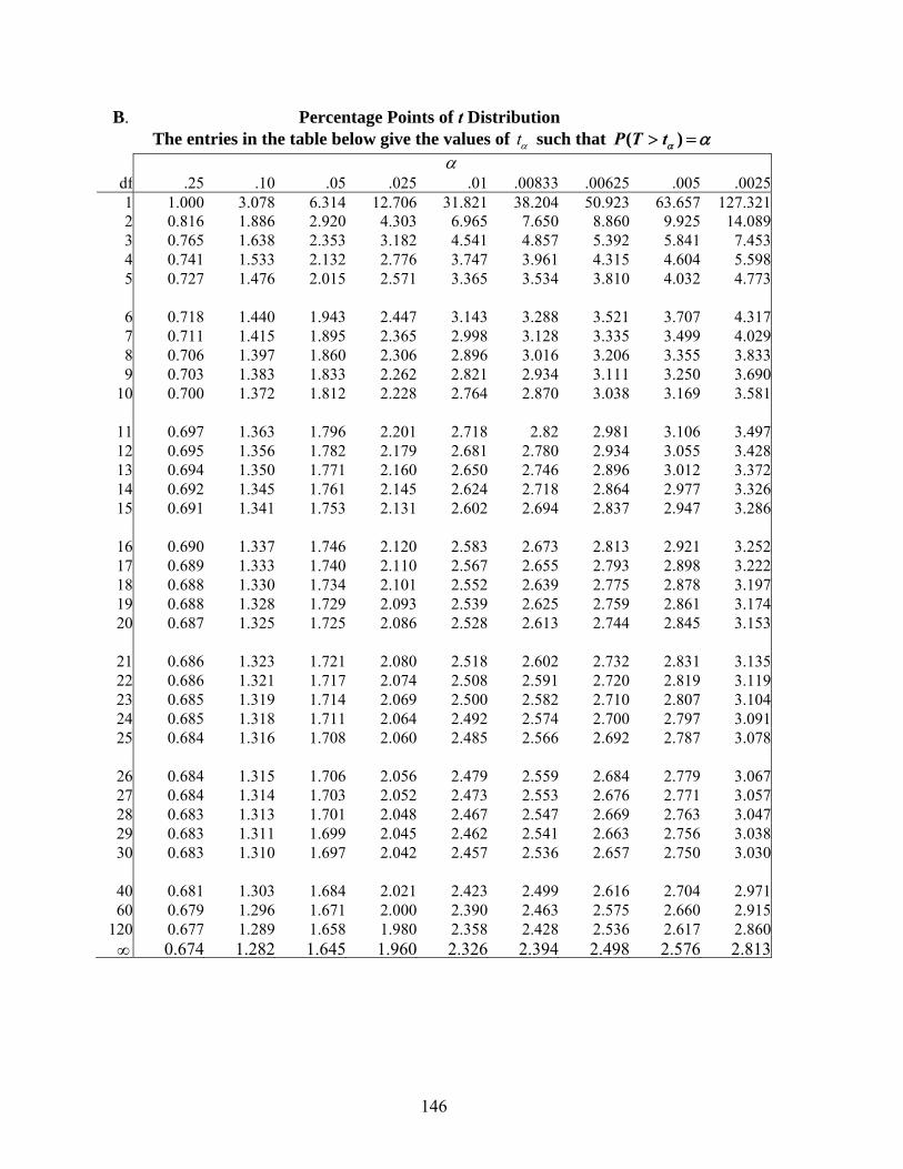
146

B. Percentage Points of t Distribution The entries in the table below give the values of tα such that ( )P T tα α> =

α df .25 .10 .05 .025 .01 .00833 .00625 .005 .00251 1.000 3.078 6.314 12.706 31.821 38.204 50.923 63.657 127.3212 0.816 1.886 2.920 4.303 6.965 7.650 8.860 9.925 14.0893 0.765 1.638 2.353 3.182 4.541 4.857 5.392 5.841 7.4534 0.741 1.533 2.132 2.776 3.747 3.961 4.315 4.604 5.5985 0.727 1.476 2.015 2.571 3.365 3.534 3.810 4.032 4.773

6 0.718 1.440 1.943 2.447 3.143 3.288 3.521 3.707 4.3177 0.711 1.415 1.895 2.365 2.998 3.128 3.335 3.499 4.0298 0.706 1.397 1.860 2.306 2.896 3.016 3.206 3.355 3.8339 0.703 1.383 1.833 2.262 2.821 2.934 3.111 3.250 3.690

10 0.700 1.372 1.812 2.228 2.764 2.870 3.038 3.169 3.581

11 0.697 1.363 1.796 2.201 2.718 2.82 2.981 3.106 3.49712 0.695 1.356 1.782 2.179 2.681 2.780 2.934 3.055 3.42813 0.694 1.350 1.771 2.160 2.650 2.746 2.896 3.012 3.37214 0.692 1.345 1.761 2.145 2.624 2.718 2.864 2.977 3.32615 0.691 1.341 1.753 2.131 2.602 2.694 2.837 2.947 3.286

16 0.690 1.337 1.746 2.120 2.583 2.673 2.813 2.921 3.25217 0.689 1.333 1.740 2.110 2.567 2.655 2.793 2.898 3.22218 0.688 1.330 1.734 2.101 2.552 2.639 2.775 2.878 3.19719 0.688 1.328 1.729 2.093 2.539 2.625 2.759 2.861 3.17420 0.687 1.325 1.725 2.086 2.528 2.613 2.744 2.845 3.153

21 0.686 1.323 1.721 2.080 2.518 2.602 2.732 2.831 3.13522 0.686 1.321 1.717 2.074 2.508 2.591 2.720 2.819 3.11923 0.685 1.319 1.714 2.069 2.500 2.582 2.710 2.807 3.10424 0.685 1.318 1.711 2.064 2.492 2.574 2.700 2.797 3.09125 0.684 1.316 1.708 2.060 2.485 2.566 2.692 2.787 3.078

26 0.684 1.315 1.706 2.056 2.479 2.559 2.684 2.779 3.06727 0.684 1.314 1.703 2.052 2.473 2.553 2.676 2.771 3.05728 0.683 1.313 1.701 2.048 2.467 2.547 2.669 2.763 3.04729 0.683 1.311 1.699 2.045 2.462 2.541 2.663 2.756 3.03830 0.683 1.310 1.697 2.042 2.457 2.536 2.657 2.750 3.030

40 0.681 1.303 1.684 2.021 2.423 2.499 2.616 2.704 2.97160 0.679 1.296 1.671 2.000 2.390 2.463 2.575 2.660 2.915

120 0.677 1.289 1.658 1.980 2.358 2.428 2.536 2.617 2.860∞ 0.674 1.282 1.645 1.960 2.326 2.394 2.498 2.576 2.813