KinematicsPart I: Motion in 1 Dimension

Lana Sheridan

De Anza College

Jan 7, 2020

Last time

• introduced the course

Overview

• basic ideas about physics

• units and symbols for scaling units

• dimensional analysis

• motion in 1-dimension

• kinematic quantities

• graphs

What is Physics?

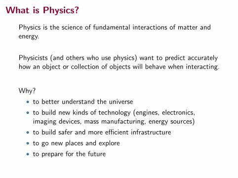
Physics is the science of fundamental interactions of matter andenergy.

Physicists (and others who use physics) want to predict accuratelyhow an object or collection of objects will behave when interacting.

Why?

• to better understand the universe

• to build new kinds of technology (engines, electronics,imaging devices, mass manufacturing, energy sources)

• to build safer and more efficient infrastructure

• to go new places and explore

• to prepare for the future

What is Physics?

Physics is the science of fundamental interactions of matter andenergy.

Physicists (and others who use physics) want to predict accuratelyhow an object or collection of objects will behave when interacting.

Why?

• to better understand the universe

• to build new kinds of technology (engines, electronics,imaging devices, mass manufacturing, energy sources)

• to build safer and more efficient infrastructure

• to go new places and explore

• to prepare for the future

What is Physics?

Physics is the science of fundamental interactions of matter andenergy.

How is it done? Make a simplified model of the system of interest,then apply a principle to make a quantitative prediction.

(Philosophy) moral of the story: Physics is not about explaininghow the world actually is. It is about finding models that makecorrect predictions.

What is Physics?

Physics is the science of fundamental interactions of matter andenergy.

How is it done? Make a simplified model of the system of interest,then apply a principle to make a quantitative prediction.

(Philosophy) moral of the story: Physics is not about explaininghow the world actually is. It is about finding models that makecorrect predictions.

What is Physics?

Theory

A refined quantitative model for making predictions that has beenverified by multiple groups of researchers and is understood tohave some regime of validity.

eg. Newtonian Mechanics - very accurately predicts the motion ofbilliard balls and the motion of planets,

• but not the perihelion precession of Mercury,

• and not the behavior of electrons in atoms.

Valid when

• v << c ,

• gravitational fields are not too strong,

• distances are much bigger than `p (Planck length), etc.

What is Physics?

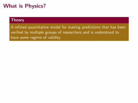
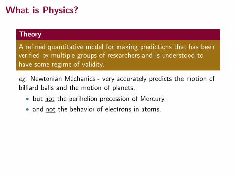
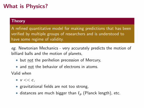
Theory

A refined quantitative model for making predictions that has beenverified by multiple groups of researchers and is understood tohave some regime of validity.

eg. Newtonian Mechanics - very accurately predicts the motion ofbilliard balls and the motion of planets,

• but not the perihelion precession of Mercury,

• and not the behavior of electrons in atoms.

Valid when

• v << c ,

• gravitational fields are not too strong,

• distances are much bigger than `p (Planck length), etc.

What is Physics?

Theory

A refined quantitative model for making predictions that has beenverified by multiple groups of researchers and is understood tohave some regime of validity.

eg. Newtonian Mechanics - very accurately predicts the motion ofbilliard balls and the motion of planets,

• but not the perihelion precession of Mercury,

• and not the behavior of electrons in atoms.

Valid when

• v << c ,

• gravitational fields are not too strong,

• distances are much bigger than `p (Planck length), etc.

What Other Physical Theories Do You Know Of?

?

Newtonian Mechanics

This course will only cover Newtonian Mechanics.

• We will look at motion from knowing the acceleration andobject experiences.

• We will analyze forces to consider what acceleration an objectwill experience.

• We will also consider the energy of a system to find itsmotion.

There are other ways of doing this analysis: Lagrangian Mechanicsand Hamiltonian Mechanics. They are not covered in the course.

Quantities, Units, MeasurementIf we want to make quantitative statements we need to agree onmeasurements: standard reference units.

We will mostly use SI (Systeme International) units:

Length meter, mMass kilogram, kgTime second, s

These base units are defined in terms of fundamental physicalphenomena - things anyone, anywhere could in principle observeconsistently.

Make sure you include the appropriate units in your answer whenyou get a number!

Also, units can be helpful for checking that your equation iscorrect.

Quantities, Units, MeasurementIf we want to make quantitative statements we need to agree onmeasurements: standard reference units.

We will mostly use SI (Systeme International) units:

Length meter, mMass kilogram, kgTime second, s

These base units are defined in terms of fundamental physicalphenomena - things anyone, anywhere could in principle observeconsistently.

Make sure you include the appropriate units in your answer whenyou get a number!

Also, units can be helpful for checking that your equation iscorrect.

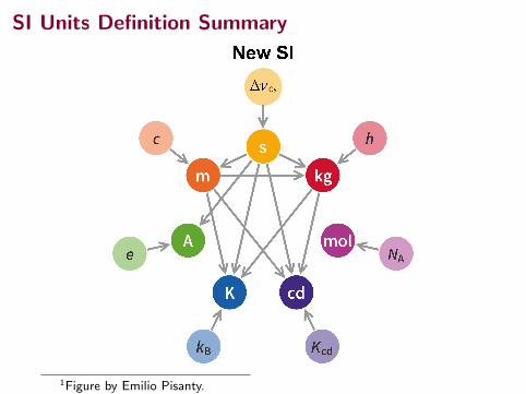
SI Units Definition Summary

1Figure by Emilio Pisanty.

SI Units Definition Summary

1Figure by Emilio Pisanty.

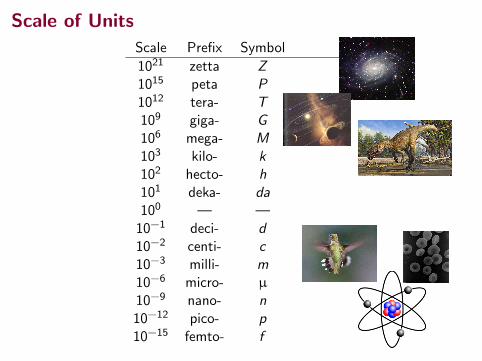
Scale of Units

Scale Prefix Symbol

1021 zetta Z1015 peta P1012 tera- T109 giga- G106 mega- M103 kilo- k102 hecto- h101 deka- da100 — —

10−1 deci- d10−2 centi- c10−3 milli- m10−6 micro- µ

10−9 nano- n10−12 pico- p10−15 femto- f

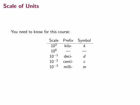
Scale of Units

You need to know for this course:

Scale Prefix Symbol

103 kilo- k100 — —

10−1 deci- d10−2 centi- c10−3 milli- m

Units are Useful: Dimensional Analysis

Considering the units or dimensions of each term on both sides ofan equation can sometimes help spot faulty equations right away.

Which of the following equations are dimensionally correct?

(1) vf = vi + ax

(2) y = (2 m) cos(kx), where k = 2 m−1.

1Serway & Jewett, Page 16, # 9.

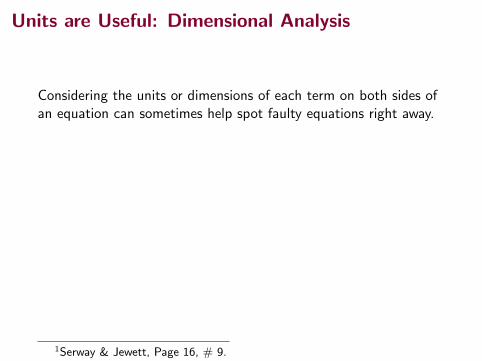
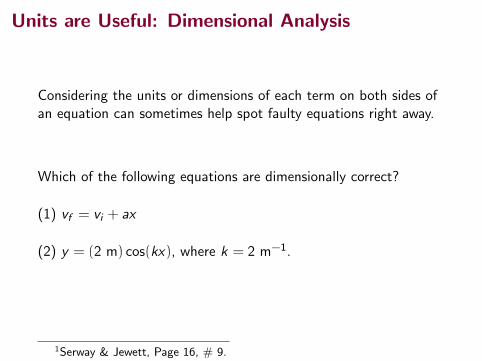
Units are Useful: Dimensional Analysis

Considering the units or dimensions of each term on both sides ofan equation can sometimes help spot faulty equations right away.

Which of the following equations are dimensionally correct?

(1) vf = vi + ax

(2) y = (2 m) cos(kx), where k = 2 m−1.

1Serway & Jewett, Page 16, # 9.

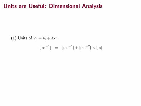
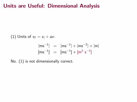
Units are Useful: Dimensional Analysis

(1) Units of vf = vi + ax :

[ms−1] = [ms−1] + [ms−2]× [m]

[ms−1] = [ms−1] + [m2 s−2]

No. (1) is not dimensionally correct.

Units are Useful: Dimensional Analysis

(1) Units of vf = vi + ax :

[ms−1] = [ms−1] + [ms−2]× [m]

[ms−1] = [ms−1] + [m2 s−2]

No. (1) is not dimensionally correct.

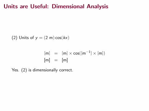
Units are Useful: Dimensional Analysis

(2) Units of y = (2 m) cos(kx)

[m] = [m]× cos([m−1]× [m])

[m] = [m]

Yes. (2) is dimensionally correct.

Kinematics: Motion in 1 Dimension

First we consider particles constrained to move only along astraight line, forwards or backwards.

Vectors

scalar

A scalar quantity indicates an amount. It is represented by a realnumber. (Assuming it is a physical quantity.)

vector

A vector quantity indicates both an amount and a direction. It isrepresented by a real number for each possible direction, or a realnumber and (an) angle(s). (Assuming it is a physical quantity.)

Vectors

scalar

A scalar quantity indicates an amount. It is represented by a realnumber. (Assuming it is a physical quantity.)

vector

A vector quantity indicates both an amount and a direction. It isrepresented by a real number for each possible direction, or a realnumber and (an) angle(s). (Assuming it is a physical quantity.)

Notation for Vectors

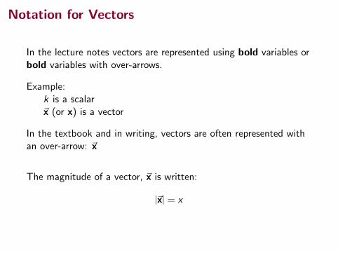
In the lecture notes vectors are represented using bold variables orbold variables with over-arrows.

Example:k is a scalar~x (or x) is a vector

In the textbook and in writing, vectors are often represented withan over-arrow: ~x

The magnitude of a vector, ~x is written:

|~x| = x

Position

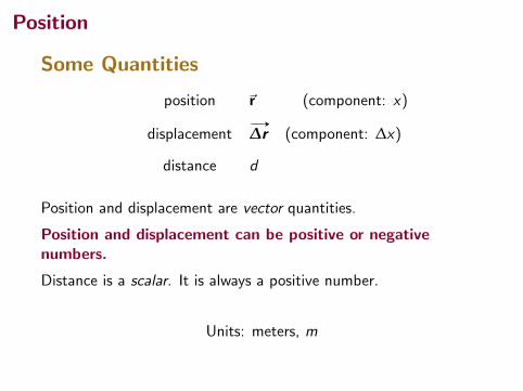
Some Quantities

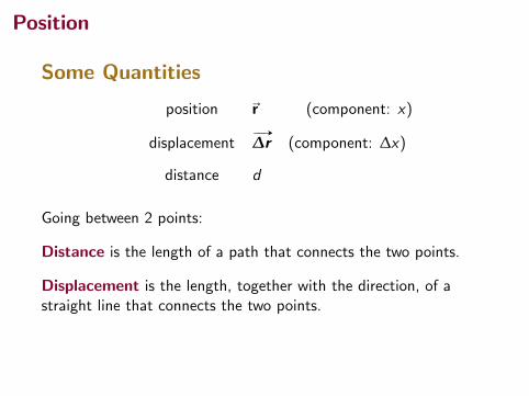
position ~r (component: x)

displacement# »

∆r (component: ∆x)

distance d

Going between 2 points:

Distance is the length of a path that connects the two points.

Displacement is the length, together with the direction, of astraight line that connects the two points.

Position

Some Quantities

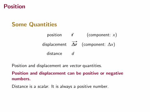
position ~r (component: x)

displacement# »

∆r (component: ∆x)

distance d

Position and displacement are vector quantities.

Position and displacement can be positive or negativenumbers.

Distance is a scalar. It is always a positive number.

Position

Some Quantities

position ~r (component: x)

displacement# »

∆r (component: ∆x)

distance d

Position and displacement are vector quantities.

Position and displacement can be positive or negativenumbers.

Distance is a scalar. It is always a positive number.

Units: meters, m

Position vs. Time Graphs

22 Chapter 2 Motion in One Dimension

obtain reasonably accurate data about its orbit. This approximation is justified because the radius of the Earth’s orbit is large compared with the dimensions of the Earth and the Sun. As an example on a much smaller scale, it is possible to explain the pressure exerted by a gas on the walls of a container by treating the gas molecules as particles, without regard for the internal structure of the molecules.

2.1 Position, Velocity, and SpeedA particle’s position x is the location of the particle with respect to a chosen ref-erence point that we can consider to be the origin of a coordinate system. The motion of a particle is completely known if the particle’s position in space is known at all times. Consider a car moving back and forth along the x axis as in Figure 2.1a. When we begin collecting position data, the car is 30 m to the right of the reference posi-tion x 5 0. We will use the particle model by identifying some point on the car, perhaps the front door handle, as a particle representing the entire car. We start our clock, and once every 10 s we note the car’s position. As you can see from Table 2.1, the car moves to the right (which we have defined as the positive direction) during the first 10 s of motion, from position ! to position ". After ", the position values begin to decrease, suggesting the car is backing up from position " through position #. In fact, at $, 30 s after we start measuring, the car is at the origin of coordinates (see Fig. 2.1a). It continues moving to the left and is more than 50 m to the left of x 5 0 when we stop recording information after our sixth data point. A graphical representation of this information is presented in Figure 2.1b. Such a plot is called a position–time graph. Notice the alternative representations of information that we have used for the motion of the car. Figure 2.1a is a pictorial representation, whereas Figure 2.1b is a graphical representation. Table 2.1 is a tabular representation of the same information. Using an alternative representation is often an excellent strategy for understanding the situation in a given problem. The ultimate goal in many problems is a math-

Position X

Position of the Car at Various Times

Position t (s) x (m)

! 0 30" 10 52% 20 38$ 30 0& 40 237# 50 253

Table 2.1

!60 !50 !40 !30 !20 !10 0 10 20 30 40 50 60x (m)

! "

The car moves to the right between positions ! and ".

!60 !50 !40 !30 !20 !10 0 10 20 30 40 50 60x (m)

$ %&#

The car moves to the left between positions % and #.

a

!

10 20 30 40 500

!40

!60

!20

0

20

40

60

"t

"x

x (m)

t (s)

"

%

$

&

#

b

Figure 2.1 A car moves back and forth along a straight line. Because we are interested only in the car’s translational motion, we can model it as a particle. Several representations of the information about the motion of the car can be used. Table 2.1 is a tabular representation of the information. (a) A pictorial representation of the motion of the car. (b) A graphical representation (position–time graph) of the motion of the car.

1Figures from Serway & Jewett

Position vs. Time Graphs

22 Chapter 2 Motion in One Dimension

obtain reasonably accurate data about its orbit. This approximation is justified because the radius of the Earth’s orbit is large compared with the dimensions of the Earth and the Sun. As an example on a much smaller scale, it is possible to explain the pressure exerted by a gas on the walls of a container by treating the gas molecules as particles, without regard for the internal structure of the molecules.

2.1 Position, Velocity, and SpeedA particle’s position x is the location of the particle with respect to a chosen ref-erence point that we can consider to be the origin of a coordinate system. The motion of a particle is completely known if the particle’s position in space is known at all times. Consider a car moving back and forth along the x axis as in Figure 2.1a. When we begin collecting position data, the car is 30 m to the right of the reference posi-tion x 5 0. We will use the particle model by identifying some point on the car, perhaps the front door handle, as a particle representing the entire car. We start our clock, and once every 10 s we note the car’s position. As you can see from Table 2.1, the car moves to the right (which we have defined as the positive direction) during the first 10 s of motion, from position ! to position ". After ", the position values begin to decrease, suggesting the car is backing up from position " through position #. In fact, at $, 30 s after we start measuring, the car is at the origin of coordinates (see Fig. 2.1a). It continues moving to the left and is more than 50 m to the left of x 5 0 when we stop recording information after our sixth data point. A graphical representation of this information is presented in Figure 2.1b. Such a plot is called a position–time graph. Notice the alternative representations of information that we have used for the motion of the car. Figure 2.1a is a pictorial representation, whereas Figure 2.1b is a graphical representation. Table 2.1 is a tabular representation of the same information. Using an alternative representation is often an excellent strategy for understanding the situation in a given problem. The ultimate goal in many problems is a math-

Position X

Position of the Car at Various Times

Position t (s) x (m)

! 0 30" 10 52% 20 38$ 30 0& 40 237# 50 253

Table 2.1

!60 !50 !40 !30 !20 !10 0 10 20 30 40 50 60x (m)

! "

The car moves to the right between positions ! and ".

!60 !50 !40 !30 !20 !10 0 10 20 30 40 50 60x (m)

$ %&#

The car moves to the left between positions % and #.

a

!

10 20 30 40 500

!40

!60

!20

0

20

40

60

"t

"x

x (m)

t (s)

"

%

$

&

#

b

Figure 2.1 A car moves back and forth along a straight line. Because we are interested only in the car’s translational motion, we can model it as a particle. Several representations of the information about the motion of the car can be used. Table 2.1 is a tabular representation of the information. (a) A pictorial representation of the motion of the car. (b) A graphical representation (position–time graph) of the motion of the car.

1Figures from Serway & Jewett

Position vs. Time Graphs

22 Chapter 2 Motion in One Dimension

obtain reasonably accurate data about its orbit. This approximation is justified because the radius of the Earth’s orbit is large compared with the dimensions of the Earth and the Sun. As an example on a much smaller scale, it is possible to explain the pressure exerted by a gas on the walls of a container by treating the gas molecules as particles, without regard for the internal structure of the molecules.

2.1 Position, Velocity, and SpeedA particle’s position x is the location of the particle with respect to a chosen ref-erence point that we can consider to be the origin of a coordinate system. The motion of a particle is completely known if the particle’s position in space is known at all times. Consider a car moving back and forth along the x axis as in Figure 2.1a. When we begin collecting position data, the car is 30 m to the right of the reference posi-tion x 5 0. We will use the particle model by identifying some point on the car, perhaps the front door handle, as a particle representing the entire car. We start our clock, and once every 10 s we note the car’s position. As you can see from Table 2.1, the car moves to the right (which we have defined as the positive direction) during the first 10 s of motion, from position ! to position ". After ", the position values begin to decrease, suggesting the car is backing up from position " through position #. In fact, at $, 30 s after we start measuring, the car is at the origin of coordinates (see Fig. 2.1a). It continues moving to the left and is more than 50 m to the left of x 5 0 when we stop recording information after our sixth data point. A graphical representation of this information is presented in Figure 2.1b. Such a plot is called a position–time graph. Notice the alternative representations of information that we have used for the motion of the car. Figure 2.1a is a pictorial representation, whereas Figure 2.1b is a graphical representation. Table 2.1 is a tabular representation of the same information. Using an alternative representation is often an excellent strategy for understanding the situation in a given problem. The ultimate goal in many problems is a math-

Position X

Position of the Car at Various Times

Position t (s) x (m)

! 0 30" 10 52% 20 38$ 30 0& 40 237# 50 253

Table 2.1

!60 !50 !40 !30 !20 !10 0 10 20 30 40 50 60x (m)

! "

The car moves to the right between positions ! and ".

!60 !50 !40 !30 !20 !10 0 10 20 30 40 50 60x (m)

$ %&#

The car moves to the left between positions % and #.

a

!

10 20 30 40 500

!40

!60

!20

0

20

40

60

"t

"x

x (m)

t (s)

"

%

$

&

#

b

Figure 2.1 A car moves back and forth along a straight line. Because we are interested only in the car’s translational motion, we can model it as a particle. Several representations of the information about the motion of the car can be used. Table 2.1 is a tabular representation of the information. (a) A pictorial representation of the motion of the car. (b) A graphical representation (position–time graph) of the motion of the car.

1Figures from Serway & Jewett

Position vs. Time Graphs

22 Chapter 2 Motion in One Dimension

obtain reasonably accurate data about its orbit. This approximation is justified because the radius of the Earth’s orbit is large compared with the dimensions of the Earth and the Sun. As an example on a much smaller scale, it is possible to explain the pressure exerted by a gas on the walls of a container by treating the gas molecules as particles, without regard for the internal structure of the molecules.

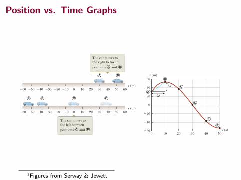
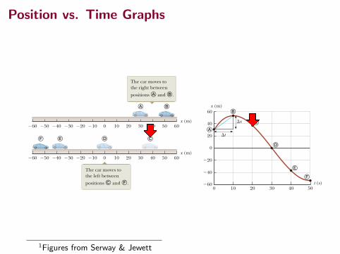
2.1 Position, Velocity, and SpeedA particle’s position x is the location of the particle with respect to a chosen ref-erence point that we can consider to be the origin of a coordinate system. The motion of a particle is completely known if the particle’s position in space is known at all times. Consider a car moving back and forth along the x axis as in Figure 2.1a. When we begin collecting position data, the car is 30 m to the right of the reference posi-tion x 5 0. We will use the particle model by identifying some point on the car, perhaps the front door handle, as a particle representing the entire car. We start our clock, and once every 10 s we note the car’s position. As you can see from Table 2.1, the car moves to the right (which we have defined as the positive direction) during the first 10 s of motion, from position ! to position ". After ", the position values begin to decrease, suggesting the car is backing up from position " through position #. In fact, at $, 30 s after we start measuring, the car is at the origin of coordinates (see Fig. 2.1a). It continues moving to the left and is more than 50 m to the left of x 5 0 when we stop recording information after our sixth data point. A graphical representation of this information is presented in Figure 2.1b. Such a plot is called a position–time graph. Notice the alternative representations of information that we have used for the motion of the car. Figure 2.1a is a pictorial representation, whereas Figure 2.1b is a graphical representation. Table 2.1 is a tabular representation of the same information. Using an alternative representation is often an excellent strategy for understanding the situation in a given problem. The ultimate goal in many problems is a math-

Position X

Position of the Car at Various Times

Position t (s) x (m)

! 0 30" 10 52% 20 38$ 30 0& 40 237# 50 253

Table 2.1

!60 !50 !40 !30 !20 !10 0 10 20 30 40 50 60x (m)

! "

The car moves to the right between positions ! and ".

!60 !50 !40 !30 !20 !10 0 10 20 30 40 50 60x (m)

$ %&#

The car moves to the left between positions % and #.

a

!

10 20 30 40 500

!40

!60

!20

0

20

40

60

"t

"x

x (m)

t (s)

"

%

$

&

#

b

Figure 2.1 A car moves back and forth along a straight line. Because we are interested only in the car’s translational motion, we can model it as a particle. Several representations of the information about the motion of the car can be used. Table 2.1 is a tabular representation of the information. (a) A pictorial representation of the motion of the car. (b) A graphical representation (position–time graph) of the motion of the car.

1Figures from Serway & Jewett

Position vs. Time Graphs

22 Chapter 2 Motion in One Dimension

obtain reasonably accurate data about its orbit. This approximation is justified because the radius of the Earth’s orbit is large compared with the dimensions of the Earth and the Sun. As an example on a much smaller scale, it is possible to explain the pressure exerted by a gas on the walls of a container by treating the gas molecules as particles, without regard for the internal structure of the molecules.

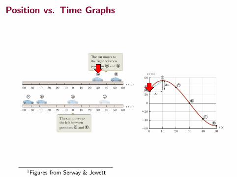
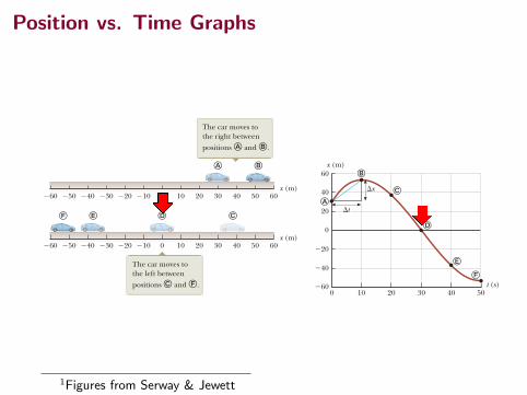
2.1 Position, Velocity, and SpeedA particle’s position x is the location of the particle with respect to a chosen ref-erence point that we can consider to be the origin of a coordinate system. The motion of a particle is completely known if the particle’s position in space is known at all times. Consider a car moving back and forth along the x axis as in Figure 2.1a. When we begin collecting position data, the car is 30 m to the right of the reference posi-tion x 5 0. We will use the particle model by identifying some point on the car, perhaps the front door handle, as a particle representing the entire car. We start our clock, and once every 10 s we note the car’s position. As you can see from Table 2.1, the car moves to the right (which we have defined as the positive direction) during the first 10 s of motion, from position ! to position ". After ", the position values begin to decrease, suggesting the car is backing up from position " through position #. In fact, at $, 30 s after we start measuring, the car is at the origin of coordinates (see Fig. 2.1a). It continues moving to the left and is more than 50 m to the left of x 5 0 when we stop recording information after our sixth data point. A graphical representation of this information is presented in Figure 2.1b. Such a plot is called a position–time graph. Notice the alternative representations of information that we have used for the motion of the car. Figure 2.1a is a pictorial representation, whereas Figure 2.1b is a graphical representation. Table 2.1 is a tabular representation of the same information. Using an alternative representation is often an excellent strategy for understanding the situation in a given problem. The ultimate goal in many problems is a math-

Position X

Position of the Car at Various Times

Position t (s) x (m)

! 0 30" 10 52% 20 38$ 30 0& 40 237# 50 253

Table 2.1

!60 !50 !40 !30 !20 !10 0 10 20 30 40 50 60x (m)

! "

The car moves to the right between positions ! and ".

!60 !50 !40 !30 !20 !10 0 10 20 30 40 50 60x (m)

$ %&#

The car moves to the left between positions % and #.

a

!

10 20 30 40 500

!40

!60

!20

0

20

40

60

"t

"x

x (m)

t (s)

"

%

$

&

#

b

Figure 2.1 A car moves back and forth along a straight line. Because we are interested only in the car’s translational motion, we can model it as a particle. Several representations of the information about the motion of the car can be used. Table 2.1 is a tabular representation of the information. (a) A pictorial representation of the motion of the car. (b) A graphical representation (position–time graph) of the motion of the car.

1Figures from Serway & Jewett

Position vs. Time Graphs

22 Chapter 2 Motion in One Dimension

obtain reasonably accurate data about its orbit. This approximation is justified because the radius of the Earth’s orbit is large compared with the dimensions of the Earth and the Sun. As an example on a much smaller scale, it is possible to explain the pressure exerted by a gas on the walls of a container by treating the gas molecules as particles, without regard for the internal structure of the molecules.

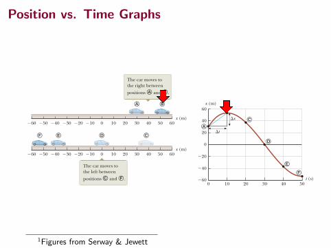
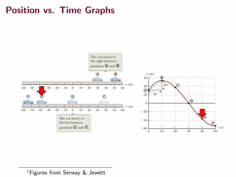
2.1 Position, Velocity, and SpeedA particle’s position x is the location of the particle with respect to a chosen ref-erence point that we can consider to be the origin of a coordinate system. The motion of a particle is completely known if the particle’s position in space is known at all times. Consider a car moving back and forth along the x axis as in Figure 2.1a. When we begin collecting position data, the car is 30 m to the right of the reference posi-tion x 5 0. We will use the particle model by identifying some point on the car, perhaps the front door handle, as a particle representing the entire car. We start our clock, and once every 10 s we note the car’s position. As you can see from Table 2.1, the car moves to the right (which we have defined as the positive direction) during the first 10 s of motion, from position ! to position ". After ", the position values begin to decrease, suggesting the car is backing up from position " through position #. In fact, at $, 30 s after we start measuring, the car is at the origin of coordinates (see Fig. 2.1a). It continues moving to the left and is more than 50 m to the left of x 5 0 when we stop recording information after our sixth data point. A graphical representation of this information is presented in Figure 2.1b. Such a plot is called a position–time graph. Notice the alternative representations of information that we have used for the motion of the car. Figure 2.1a is a pictorial representation, whereas Figure 2.1b is a graphical representation. Table 2.1 is a tabular representation of the same information. Using an alternative representation is often an excellent strategy for understanding the situation in a given problem. The ultimate goal in many problems is a math-

Position X

Position of the Car at Various Times

Position t (s) x (m)

! 0 30" 10 52% 20 38$ 30 0& 40 237# 50 253

Table 2.1

!60 !50 !40 !30 !20 !10 0 10 20 30 40 50 60x (m)

! "

The car moves to the right between positions ! and ".

!60 !50 !40 !30 !20 !10 0 10 20 30 40 50 60x (m)

$ %&#

The car moves to the left between positions % and #.

a

!

10 20 30 40 500

!40

!60

!20

0

20

40

60

"t

"x

x (m)

t (s)

"

%

$

&

#

b

Figure 2.1 A car moves back and forth along a straight line. Because we are interested only in the car’s translational motion, we can model it as a particle. Several representations of the information about the motion of the car can be used. Table 2.1 is a tabular representation of the information. (a) A pictorial representation of the motion of the car. (b) A graphical representation (position–time graph) of the motion of the car.

1Figures from Serway & Jewett

Position vs. Time Graphs

22 Chapter 2 Motion in One Dimension

obtain reasonably accurate data about its orbit. This approximation is justified because the radius of the Earth’s orbit is large compared with the dimensions of the Earth and the Sun. As an example on a much smaller scale, it is possible to explain the pressure exerted by a gas on the walls of a container by treating the gas molecules as particles, without regard for the internal structure of the molecules.

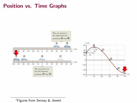
2.1 Position, Velocity, and SpeedA particle’s position x is the location of the particle with respect to a chosen ref-erence point that we can consider to be the origin of a coordinate system. The motion of a particle is completely known if the particle’s position in space is known at all times. Consider a car moving back and forth along the x axis as in Figure 2.1a. When we begin collecting position data, the car is 30 m to the right of the reference posi-tion x 5 0. We will use the particle model by identifying some point on the car, perhaps the front door handle, as a particle representing the entire car. We start our clock, and once every 10 s we note the car’s position. As you can see from Table 2.1, the car moves to the right (which we have defined as the positive direction) during the first 10 s of motion, from position ! to position ". After ", the position values begin to decrease, suggesting the car is backing up from position " through position #. In fact, at $, 30 s after we start measuring, the car is at the origin of coordinates (see Fig. 2.1a). It continues moving to the left and is more than 50 m to the left of x 5 0 when we stop recording information after our sixth data point. A graphical representation of this information is presented in Figure 2.1b. Such a plot is called a position–time graph. Notice the alternative representations of information that we have used for the motion of the car. Figure 2.1a is a pictorial representation, whereas Figure 2.1b is a graphical representation. Table 2.1 is a tabular representation of the same information. Using an alternative representation is often an excellent strategy for understanding the situation in a given problem. The ultimate goal in many problems is a math-

Position X

Position of the Car at Various Times

Position t (s) x (m)

! 0 30" 10 52% 20 38$ 30 0& 40 237# 50 253

Table 2.1

!60 !50 !40 !30 !20 !10 0 10 20 30 40 50 60x (m)

! "

The car moves to the right between positions ! and ".

!60 !50 !40 !30 !20 !10 0 10 20 30 40 50 60x (m)

$ %&#

The car moves to the left between positions % and #.

a

!

10 20 30 40 500

!40

!60

!20

0

20

40

60

"t

"x

x (m)

t (s)

"

%

$

&

#

b

Figure 2.1 A car moves back and forth along a straight line. Because we are interested only in the car’s translational motion, we can model it as a particle. Several representations of the information about the motion of the car can be used. Table 2.1 is a tabular representation of the information. (a) A pictorial representation of the motion of the car. (b) A graphical representation (position–time graph) of the motion of the car.

1Figures from Serway & Jewett

Summary

• some quantities for describing motion: position ~r, velocity ~v,time t

• position, displacement, and velocity are vector quantities(have signs)

• distance and speed are scalar quantities (always positive)

• we can plot these quantities against time

Quiz Friday, start of class

(Uncollected) HomeworkSerway & Jewett,

• Ch 1, onward from page 14. Problems: 9, 45, 57, 67, 71

• Ch 2, onward from page 49. Obj. Q: 1; CQ: Concep. Q: 1;Probs: 1, 3, 7, 11